c� COPYRIGHT

by

Ryan C. Briggs

2013

ALL RIGHTS RESERVED

ii

AIDING AND ABETTING: THE INFLUENCE OF

FOREIGN ASSISTANCE ON INCUMBENT

ADVANTAGE IN AFRICAby

Ryan C. Briggs

ABSTRACT

Can changes in foreign aid influence incumbent advantage in aid-recipient coun-

tries? This dissertation suggests that in post-Cold War Africa, the answer is yes. The

argument rests on a cross-national analysis of all African elections between 1990 and

2006 and three case studies of African elections. The cross-national analysis demon-

strates a durable correlation between changes in aid and incumbent advantage. Case

studies of elections in Ghana in 2000, Malawi in 1999, and Kenya in 1992 present

subnational confirmation of the main findings and flush out the mechanisms that

link aid changes to incumbent advantage. The dissertation thus demonstrates that

foreign aid volatility influences election results in Africa, that aid recipients often are

able to use an electoral logic to strategically target aid, and that African voters are

influenced by the provision of goods and services.

iii

ACKNOWLEDGEMENTS

I owe considerable gratitude to the many people who helped to produce this

dissertation. Firstly, I owe a debt to everyone who provided me with data or who

helped me while I was overseas. In Ghana, I would like to thank to Emmanuel

Gyimah-Boadi and Victor Brobbey at the Centre for Democratic Development for

helping me get my sea legs as I started field work. Ed Carr was also generous with

contacts and advice. Julius and Solomon and the Ministry of Energy were incredibly

helpful in locating data on electrification. Finally, Kevin Fridy and Afua Branoah

Banful were generous with their data.

In Kenya, Paul Kamau at the Institute for Development Studies at the Uni-

versity of Nairobi helped me become an a�liate scholar at IDS, opening many doors.

Chris Namachanja, Joseph Wambua, and Moses Kiptui at the Kenya School of Mon-

etary Studies provided useful discussions and a wealth of contacts. Discussion with

Terry Ryan at the Central Bank was very helpful in understanding Kenyan poli-

cymaking in the 1990s. While in Kenya, Peter Kimani Muhia provided excellent

research assistance. While in Nairobi I was also a participant in the American Po-

litical Science Africa Workshop. I would like to thanks all participants for creating

such a wonderful, intellectually stimulating atmosphere and APSA for making the

workshop possible.

In Malawi, Rexie Chiluzi, the Assistant Auditor General at the National Audit

O�ce, helped me track down old reports that ended up being important to the final

argument of the chapter. King Norman Rudi at the Malawi Electoral Commission

iv

was a model of e�ciency and openness. In Lilongwe, I had a very useful discussion

with Henry Chinpaige about elections and campaign financing. Seeing his finished

dissertation helped me stay motivated. Ephraim Chirwa and Blessings Chinsinga at

Chancellor College were kind enough share their time and deep knowledge of Malawi

with me. I cannot thank Charles Clark at the Malawi Starter Pack Logistic Unit

enough for taking the time to dig around his garage over a weekend in order to

find records of fertilizer subsidy transfers that were on five floppy disks. Last, but

certainly not least, Kim Yi Dionne was kind enough to share her data on Malawi’s

election results.

I am grateful to American University, the Cosmos Club, and the Social Sciences

and Humanities Research Council of Canada for financial support during both my

time overseas and in Washington. Their support gave me the ability not only to

thoroughly examine my topic but managed to feed me and house me during this

period as well.

I owe much gratitude to those at the School of International Service, who have

supported and nurtured me over the last five years. There have been many classes,

professors and students who have shaped this final product in ways that I cannot

begin express. In particular, my cohort at SIS has been instrumental in keeping me

motivated. I owe particular thanks to Sebastian Bitar and Tom Long. Sebastian

has helped me shape my thoughts immeasurably through many intense discussions

and has provided much needed stress relief on the squash court. Tom has carefully

read almost everything I have written over the last five years, a service that requires

thanks both on my behalf and on the behalf of any readers. I must also thank him

for much intellectually stimulating time in the bar, although it may have resulted in

a headache or two.

In addition, I would be remiss if I did not also thanks Patrick Jackson, who

v

read much of my work and was always willing to respond to emails about obscure

methodological debates at odd hours.

Most vital to my academic success have been my committee: Deborah Brautigam,

Barak Ho↵man, and Carl LeVan. Carl has been both a careful reader and a mentor.

I spent more time arguing with Barak than anyone else, and the dissertation is better

for it. Deborah was my reason for coming to American University and was involved

in every step of the dissertation. Her time and attention are reflected in the better

parts of the writing.

Finally, I would like to thank my family. I owe my parents much gratitude

for always supporting me. I’d also like to thank Matthew for giving me a reason to

finish quickly. Most importantly, I would like to thank my wife. Maya, your support,

attention, wit, criticisms, and baking helped ensure that this process was as painless

as possible. I love you tremendously.

vi

TABLE OF CONTENTS

ABSTRACT . . . . . . . . . . . . . . . . . . . . . . . . . . . . . . . . . . . . ii

ACKNOWLEDGEMENTS . . . . . . . . . . . . . . . . . . . . . . . . . . . . iii

LIST OF TABLES . . . . . . . . . . . . . . . . . . . . . . . . . . . . . . . . . x

LIST OF FIGURES . . . . . . . . . . . . . . . . . . . . . . . . . . . . . . . . xii

CHAPTER

1. INTRODUCTION . . . . . . . . . . . . . . . . . . . . . . . . . . . . . 1

1.1 Why Might Foreign Aid Work? . . . . . . . . . . . . . . . . . . . 3

1.2 Why aid matters . . . . . . . . . . . . . . . . . . . . . . . . . . . 5

1.3 Why aid matters for African democracies . . . . . . . . . . . . . 8

1.4 Discourses on Aid . . . . . . . . . . . . . . . . . . . . . . . . . . 10

1.5 Outline . . . . . . . . . . . . . . . . . . . . . . . . . . . . . . . . 13

2. THEORY AND METHODOLOGY . . . . . . . . . . . . . . . . . . . 14

2.1 What we know about aid and political survival . . . . . . . . . . 14

2.2 Why aid might boost votes . . . . . . . . . . . . . . . . . . . . . 15

2.2.1 The public goods mechanism . . . . . . . . . . . . . . . . . . 15

2.2.2 The private goods mechanism . . . . . . . . . . . . . . . . . . 19

2.2.3 Other ways that aid could influence voters . . . . . . . . . . . 20

2.3 Political targeting: Who controls aid? . . . . . . . . . . . . . . . 23

2.4 Methods . . . . . . . . . . . . . . . . . . . . . . . . . . . . . . . 29

2.4.1 Scope Conditions . . . . . . . . . . . . . . . . . . . . . . . . 29

vii

2.4.2 Aid Changes Across Countries . . . . . . . . . . . . . . . . . 30

2.4.3 Investigating Causality and Causal Mechanisms with Cases . 31

2.4.4 A note on data . . . . . . . . . . . . . . . . . . . . . . . . . . 32

2.5 The plan for the remainder of the dissertation . . . . . . . . . . . 34

3. CROSS NATIONAL EVIDENCE . . . . . . . . . . . . . . . . . . . . 35

3.1 Data . . . . . . . . . . . . . . . . . . . . . . . . . . . . . . . . . . 36

3.2 Initial Analysis . . . . . . . . . . . . . . . . . . . . . . . . . . . . 39

3.3 Evidence that aid changes influence incumbent advantage . . . . 42

3.4 Multicollinearity and Sensitivity Tests . . . . . . . . . . . . . . . 49

3.5 Evidence that di↵erent regimes are a↵ected di↵erently . . . . . . 51

3.6 Picking cases . . . . . . . . . . . . . . . . . . . . . . . . . . . . . 55

3.6.1 Ghana, 2000 . . . . . . . . . . . . . . . . . . . . . . . . . . . 56

3.6.2 Malawi, 1999 . . . . . . . . . . . . . . . . . . . . . . . . . . . 56

3.6.3 Kenya, 1992 . . . . . . . . . . . . . . . . . . . . . . . . . . . 57

3.6.4 Case Selection Summary . . . . . . . . . . . . . . . . . . . . 57

3.7 Conclusion . . . . . . . . . . . . . . . . . . . . . . . . . . . . . . 58

4. GHANA . . . . . . . . . . . . . . . . . . . . . . . . . . . . . . . . . . 64

4.1 Who Supported the NDC in the 1990s and Why? . . . . . . . . . 66

4.2 The NDC’s Allocative Strategies . . . . . . . . . . . . . . . . . . 71

4.3 The Causes and E↵ects of Aid in Ghana . . . . . . . . . . . . . . 73

4.3.1 The National Electrification Project . . . . . . . . . . . . . . 74

4.3.2 Targeting at the Regional Level . . . . . . . . . . . . . . . . 74

4.3.3 Targeting at the Constituency Level . . . . . . . . . . . . . . 80

4.3.4 Electoral E↵ects of Constituency-level Targeting . . . . . . . 85

4.3.5 Validity and the Counter Factual . . . . . . . . . . . . . . . . 88

4.4 Conclusion . . . . . . . . . . . . . . . . . . . . . . . . . . . . . . 93

viii

5. MALAWI . . . . . . . . . . . . . . . . . . . . . . . . . . . . . . . . . 96

5.1 General political history leading up to 1999 election . . . . . . . 97

5.1.1 History of Malawian fiscal policy and the influence of aid . . 98

5.1.2 The 1999 Election . . . . . . . . . . . . . . . . . . . . . . . . 101

5.2 How could aid have influenced the 1999 election? . . . . . . . . . 102

5.2.1 Where would Muluzi target aid? . . . . . . . . . . . . . . . . 104

5.3 Malawi Social Action Fund . . . . . . . . . . . . . . . . . . . . . 104

5.3.1 Targeting MASAF CSP Funds . . . . . . . . . . . . . . . . . 106

5.3.2 Targeting MASAF PWP Funds . . . . . . . . . . . . . . . . . 110

5.3.3 The e↵ects of MASAF spending on voting behaviour . . . . . 111

5.4 Actual Improvements in the Provision of Primary Education . . . 115

5.5 Corruption surrounding school construction . . . . . . . . . . . . 118

5.6 Conclusion . . . . . . . . . . . . . . . . . . . . . . . . . . . . . . 123

6. KENYA . . . . . . . . . . . . . . . . . . . . . . . . . . . . . . . . . . 126

6.1 Context . . . . . . . . . . . . . . . . . . . . . . . . . . . . . . . . 127

6.1.1 Domestic Context . . . . . . . . . . . . . . . . . . . . . . . . 127

6.1.2 International Context . . . . . . . . . . . . . . . . . . . . . . 129

6.1.3 The 1992 Election Results . . . . . . . . . . . . . . . . . . . . 136

6.2 Data Quality and Empirical Strategy . . . . . . . . . . . . . . . . 139

6.3 Moi’s Survival Strategies . . . . . . . . . . . . . . . . . . . . . . 140

6.3.1 The Geography of Development Spending . . . . . . . . . . . 141

6.3.2 Macroeconomic Survival Strategies . . . . . . . . . . . . . . . 149

6.3.3 Theft, Fraud, and Violence . . . . . . . . . . . . . . . . . . . 152

6.4 Conclusion . . . . . . . . . . . . . . . . . . . . . . . . . . . . . . 160

6.4.1 Explaining Moi’s response to the aid cut . . . . . . . . . . . . 160

6.4.2 Kenya in comparative perspective . . . . . . . . . . . . . . . 161

ix

7. CONCLUSION . . . . . . . . . . . . . . . . . . . . . . . . . . . . . . 164

7.1 Aid and Distributive Politics in Africa . . . . . . . . . . . . . . . 167

7.2 Foreign aid and Democracy . . . . . . . . . . . . . . . . . . . . . 170

7.3 Closing thoughts . . . . . . . . . . . . . . . . . . . . . . . . . . . 171

APPENDIX

A. AN AGENT-BASED MODEL OF THE AID SYSTEM . . . . . . . . 173

A.1 Aid Volatility and Agent-Based Models . . . . . . . . . . . . . . 173

A.1.1 Why Does Aid Volatility Exist . . . . . . . . . . . . . . . . . 174

A.1.2 Why Model? . . . . . . . . . . . . . . . . . . . . . . . . . . . 175

A.1.3 Testing Models . . . . . . . . . . . . . . . . . . . . . . . . . . 176

A.1.4 NetLogo Basics . . . . . . . . . . . . . . . . . . . . . . . . . . 178

A.1.5 Motivations behind the model . . . . . . . . . . . . . . . . . 179

A.1.6 Macrocharacteristics of the aid system . . . . . . . . . . . . . 180

A.2 The Setup of the Model . . . . . . . . . . . . . . . . . . . . . . . 180

A.2.1 Main Simulation Loop . . . . . . . . . . . . . . . . . . . . . . 182

A.3 Results . . . . . . . . . . . . . . . . . . . . . . . . . . . . . . . . 185

A.3.1 Macro Behavior . . . . . . . . . . . . . . . . . . . . . . . . . 186

A.3.2 Recipient-Level Behavior . . . . . . . . . . . . . . . . . . . . 190

A.3.3 Shocks to the System . . . . . . . . . . . . . . . . . . . . . . 193

A.3.4 Adding a Multilateral Donor . . . . . . . . . . . . . . . . . . 195

A.4 Conclusion . . . . . . . . . . . . . . . . . . . . . . . . . . . . . . 197

x

LIST OF TABLES

Table Page

2.1. The Expected Influence of Aid Across Regime Types . . . . . . . . . 28

2.2. Case Selection Summary . . . . . . . . . . . . . . . . . . . . . . . . . 32

3.1. Extreme Changes in Aid and Election Outcomes . . . . . . . . . . . . 42

3.2. Regressions Without Outliers . . . . . . . . . . . . . . . . . . . . . . 47

3.3. Sectors under Analysis in Cases . . . . . . . . . . . . . . . . . . . . . 58

3.4. Elections dropped from Sta↵an Lindberg’s Dataset . . . . . . . . . . 60

3.5. Recoded Elections from Sta↵an Lindberg’s Dataset . . . . . . . . . . 61

3.6. Regressions with outliers . . . . . . . . . . . . . . . . . . . . . . . . . 62

3.7. Two-turnover Interaction Term Regressions . . . . . . . . . . . . . . . 63

4.1. Determinants of NEP Funding to Regions . . . . . . . . . . . . . . . 77

4.2. Comparisons within ordinary districts . . . . . . . . . . . . . . . . . . 82

4.3. Comparisons between municipal and ordinary districts . . . . . . . . 83

4.4. Constituencies and Electrification status in Upper West and Upper East 83

4.5. Rural and Urban Electrification Rates in 2000 . . . . . . . . . . . . . 91

5.1. 1994 Legislative Election Results . . . . . . . . . . . . . . . . . . . . 102

5.2. 1999 Legislative Election Results . . . . . . . . . . . . . . . . . . . . 102

5.3. MASAF Proposals and Approvals . . . . . . . . . . . . . . . . . . . . 106

5.4. Relationship between CSP Cost-Sharing and UDF Voting in 1994 . . 109

5.5. Relationship between per kilometer PWP Road funding in 1998 andUDF Voting in 1994 . . . . . . . . . . . . . . . . . . . . . . . . . . . 111

xi

5.6. Relationship between PWP Road funding and UDF Voting in 1999 . 113

5.7. Relationship between Educational Variables and UDF Voting in 1999 117

6.1. Determinants of Health Resources . . . . . . . . . . . . . . . . . . . . 147

A.1. Summary of Main Variables . . . . . . . . . . . . . . . . . . . . . . . 182

A.2. Summary of Random Changes . . . . . . . . . . . . . . . . . . . . . . 184

A.3. Volatility and the Number of the Actors in the Systema . . . . . . . . 189

A.4. How Volatility Responds to Need Shocksa . . . . . . . . . . . . . . . 194

A.5. How Multilateral Donors Influence Aid Volatilitya . . . . . . . . . . . 197

xii

LIST OF FIGURES

Figure Page

1.1. Aid Volatility in Africa . . . . . . . . . . . . . . . . . . . . . . . . . . 6

2.1. How divisibility enables domestic targeting. . . . . . . . . . . . . . . 26

3.1. Incumbent Wins and Losses Across Africa by Year . . . . . . . . . . . 37

3.2. Mean Pre-electoral Aid Levels, Grouped by Election Outcome. . . . . 40

3.3. Di↵erences in Electoral Failure of Incumbents, Grouped by the Mag-nitude of the Change in Aid . . . . . . . . . . . . . . . . . . . . . . . 41

3.4. Outliers in the Aid Change variable . . . . . . . . . . . . . . . . . . . 45

3.5. The Outlier-Free Relationship Between Aid Change and PredictedIncumbent Loss . . . . . . . . . . . . . . . . . . . . . . . . . . . . . . 46

3.6. ROC curve for Model 1, without outliers . . . . . . . . . . . . . . . . 51

4.1. Explaining NEP resource allocation with the size of each region. . . 76

4.2. Explaining NEP resource allocation with the size of each region. . . 78

4.3. Mean NDC vote across rural constituencies in Upper West and UpperEast, grouped by electrification status. . . . . . . . . . . . . . . . . . 84

4.4. Mean NDC vote change across rural constituencies in Upper West andUpper East, grouped by electrification status. . . . . . . . . . . . . . 87

4.5. Regional Variation in Access to Electricity in 1991/92 (Ghana Statis-tical Service, 1992). . . . . . . . . . . . . . . . . . . . . . . . . . . . 95

5.1. Foreign Grants and Malawian Government Expenditure . . . . . . . 100

5.2. District-Level Maps of Vote Changes and Various Indicators, darkerdistricts indicate more of the indicator . . . . . . . . . . . . . . . . . 114

6.1. The Form and Magnitude of Disbursed Aid to Kenya . . . . . . . . . 134

xiii

6.2. Kenyan Expected and Received Net External Financing . . . . . . . 135

6.3. Road Resources Allocated to Moi’s base . . . . . . . . . . . . . . . . 143

6.4. Road Resources Allocated to Kenyatta’s base . . . . . . . . . . . . . 144

6.5. Road Resources Allocated to the Remainder of Kenya . . . . . . . . 145

6.6. Sources of Kenyan Government Deficit Financing . . . . . . . . . . . 150

7.1. Aid to Africa is Still Important . . . . . . . . . . . . . . . . . . . . . 165

7.2. Di↵erences in Electoral Failure of Incumbents, Grouped by the Mag-nitude of the Change in Aid . . . . . . . . . . . . . . . . . . . . . . . 167

A.1. A sample of the code used in this ABM . . . . . . . . . . . . . . . . . 178

A.2. An example of the user’s view of the interface after one simulation . . 186

A.3. Actual Volatility in Aid over Time . . . . . . . . . . . . . . . . . . . 188

A.4. Constant Dollar ODA Disbursements to Three Countries in Africa . . 191

A.5. The First Three Donors in One Simulation . . . . . . . . . . . . . . . 192

A.6. One country experiences a need shock . . . . . . . . . . . . . . . . . . 195

1

CHAPTER 1

INTRODUCTION

There is an expression in Swahili: haraka haraka haina baraka. It is rarely

used anymore, but everyone knows it. It means “hurry hurry has no blessing.”1 The

value of this expression became known to me when I was traveling to Kilwa Masoko,

a town on the coast in Southern Tanzania. I was traveling 200 miles, but the trip

took about eight hours. I have traveled on many rural roads, but this was one of the

worst rides I have ever had the displeasure of taking. At one point, we went over an

especially large bump and my wife managed to pop o↵ her seat and drive her head

into the plastic luggage rack above us, leaving a fairly large hole. This incident was

unexpectedly funny and made her wildly popular with our fellow passengers, but it

did little to increase my opinion of the road. This road was not falling apart from

neglect however. It was simply “under construction.”

Whether poor roads are fixed, and how long that construction takes, are typi-

cally considered core questions of state capacity. If a road is fixed quickly, then your

state is doing a good job. If a road is neglected or construction drags on then the state

is doing something wrong. We like to think that there is some relationship between

things getting better and domestic politics; if we vote for the right person or the

right party, services and quality of life will improve. If things are not getting better

1The common meaning is “slow down and enjoy life”.

2

then the government is failing, and accordingly voters can remove that government

from power. Governments should fear being removed from power, and so strive to do

a good job. While these domestic accountability relationships may be present, they

are not always the most important factor driving either the electoral calculations

of voters or citizens. It seems hard to believe that the delated construction on this

quiet road carrying people who have likely never left Tanzania has everything to do

with things that happen thousands of miles away. But it does. This road was under

construction thanks to aid money, and it seems likely that reliance on foreign aid

was also a factor explaining the lethargic pace of construction.

This dissertation shows firstly that when people in low-income countries vote

they are partially influenced by the quality and quantity of goods and services that

their governments (or donors) provide. Furthermore, these services, including this

road, are a↵ected by changes in aid given by foreign donors. As we would expect,

more aid typically means better roads, schools and electricity while less aid means

fewer services. What is surprising is that changes in aid are generally not the result

of a coordinated e↵ort by donors to support those who promote democracy or to

penalize countries that ignore the needs of their citizens. Instead, these shocks are

largely random.2 The people who use this road every day are the people who will

vote for the next president of Tanzania. When they do, they will look at the road

and other infrastructure, and ask ‘Did the current president do anything to improve

this infrastructure? Will someone else do a better job?’ Aid is volatile, and this

volatility can a↵ect the rollout of public works. Citizens often judge incumbents on

their ability to build public works or to provide other state services. This means

that international aid volatility is wired into the electoral outcomes of aid recipients

2The shocks are generally random from the point of view of the aid recipient. They aregenerally influenced by domestic politics in the donor country. This is discussed further below.

3

in Africa.

1.1 Why Might Foreign Aid Work?

Before delving into the volatility of foreign aid, it is useful to recap why it

is given and what it typically aims to do. To some extent, the answer to these

questions will depend on who you ask. For an economist, aid typically aims to

add to low savings (and thus investment) rates in aid-recipient countries. When an

economist asks whether or not aid works, she is typically asking a question about

economic growth. In theory, foreign aid could increase economic growth if low-income

countries had their growth constrained by low investment and low savings. This low

investment would result in the slower uptake of technology, which is a fundamental

driver of economic growth.3 Roughly the same argument can be applied not only to

new technologies like machines but also to improving the productivity of people. Here

aid might work because it increases education or health outcomes, and healthier and

better educated workers are more productive. There are strong theoretical arguments

for both claims, although the empirical evidence of aid leading to economic growth

seems to be weak (Easterly, 2001; Roodman, 2007).

While international relations scholars have generally given aid less thought,

those that have looked at foreign aid have often seen it as simply another way to

accomplish the donor state’s goals in international politics. In this view, states

sometimes have international goals that are best accomplished through the transfer of

resources from one country to another (Morgenthau, 1962). There is some empirical

support for this idea. For example, if a low-income country gets a temporary seat at

the UN Security Council, it tends to see its level of foreign aid increase (Kuziemko

3This is especially clear in the Harrod-Domar growth model. While this mode is outdated,it still strongly influences thinking about appropriate foreign aid levels (e.g. Clemens and Moss,2005).

4

and Werker, 2006). Aid allocations are also driven by other political and historical

factors. For example, former colonial ties, alliances, and measures of recipient need

explain a great deal of the variance in the level of aid that donors give to recipients.

(Alesina and Dollar, 2000).

Interestingly, the factors that influence year-to-year changes in aid are largely

independent of the factors that influence overall aid levels.4 There are fewer anal-

yses of aid changes than aid levels, but a few results stand out. The first is that

after holding other factors constant, countries that become more democratic see an

increase in aid (Alesina and Dollar, 2000). The second is that changes in corruption

are not punished by reductions in aid (Alesina and Weder, 2002).5 There is also

some limited evidence that donors can change aid allocations in response to recipi-

ent election cycles. Dreher and Jensen (2007) show that US allies receive IMF loans

with fewer conditions when they are in election years. In a working paper, Faye

and Niehaus (2010) show that if a recipient country administration is more aligned

with a donor, then they tend to receive more aid in an election year than would

otherwise be expected.6 However, even if individual donors sometimes engage in

election targeting, Kharas and Desai (2010) found that overall, electioneering does

not a↵ect aid allocations: “We do not find that electioneering plays a significant role

in aid volatility, as countries experiencing elections do not tend to experience greater

volatility than those who are not” (Kharas and Desai, 2010, p. 13).

Whatever the goals of aid, it has become a major source of finance for low-

income countries. Since the end of the Cold War, countries in Africa have cumu-

4Many of the factors that determine aid levels are slow changing (alliance patterns) orhistorical (colonial ties) and so cannot explain changes.

5In fact, larger volumes of aid are positively correlated with corruption, though causalitycould flow in either direction.

6Both studies use UN voting records to measure alignment.

5

latively received tens of billions of dollars of o�cial development assistance (ODA),

defined by the Organisation for Economic Co-operation and Development (OECD)

as non-military assistance that is provided at concessional interest rates (OECD,

2010). This number is especially large when compared to most aid recipients’ gross

domestic products or government budgets. In 1999 in Malawi, for instance, foreign

aid equaled 89% of government expenditure (Brautigam and Knack, 2004). In many

low-income countries, foreign donors regularly spend more on development than re-

cipient governments.

1.2 Why aid matters

This reliance on aid is troubling for a few reasons. First, many of the countries

that are high-income today are thought to have become rich because they had politi-

cal institutions that allowed for creative destruction and economic growth (Acemoglu

and Robinson, 2012). While there are many di↵erent pathways to open and inclusive

political institutions, one common pathway stresses the role of domestic taxation in

restraining governments (e.g. North and Weingast, 1989; Tilly, 1992). One potential

problem with aid, like other sources of ‘free money’ like oil, is that it might break

the financial reliance of governments on citizens and thus reduce the accountability

of governments to citizens (Moore, 2001).

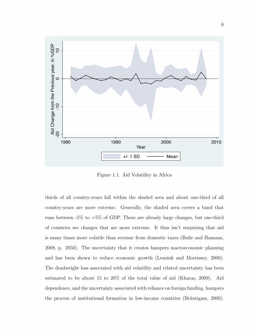
A second problem with aid is simply that it is a very volatile source of funding.

Figure 1.1 graphs aid changes from the previous year to all countries in sub-Saharan

Africa over time.7 The changes are expressed as a fraction of the recipient’s GDP.

The mean aid change is about zero, which makes sense given that some each year

some countries see increases and some experience decreases. The shaded area of

the graphs covers one standard deviation above and below the mean. About two-

7Aid here is net ODA disbursements less technical assistance and debt relief.

6

-20

-10

010

Aid

Cha

nge

from

the

Prev

ious

yea

r, in

%G

DP

1980 1990 2000 2010Year

+/- 1 SD Mean

Figure 1.1. Aid Volatility in Africa

thirds of all country-years fall within the shaded area and about one-third of all

country-years are more extreme. Generally, the shaded area covers a band that

runs between -5% to +5% of GDP. These are already large changes, but one-third

of countries see changes that are more extreme. It thus isn’t surprising that aid

is many times more volatile than revenue from domestic taxes (Bulir and Hamann,

2008, p. 2050). The uncertainty that it creates hampers macroeconomic planning

and has been shown to reduce economic growth (Lensink and Morrissey, 2000).

The deadweight loss associated with aid volatility and related uncertainty has been

estimated to be about 15 to 20% of the total value of aid (Kharas, 2009). Aid

dependence, and the uncertainty associated with reliance on foreign funding, hampers

the process of institutional formation in low-income countries (Brautigam, 2000).

7

Despite these problems, aid volatility is not decreasing over time (Bulir and Hamann,

2008).

While there have been surprisingly little empirical work on the causes of aid

volatility, there are some plausible explanations for its persistence. The dominant

theory is that there are too many donors active in each recipient country and the

donors do not coordinate well.8 Another related explanation is that recipients have

no way to punish donors for volatility and donors have no other incentive to more ef-

fectively tie their hands and commit themselves to hitting their disbursement targets.

This implies that aid recipients have very little influence over the level of volatility

that they experience and that they usually will be unable to predict when they are

likely to experience aid fluctuations. This is borne out by the only study that explic-

itly analyzed the causes of aid volatility. In it, the authors note that “all in all, there

are relatively few recipient-country traits that influence volatility in a consistent

manner” (Kharas and Desai, 2010, p. 24). This means that the bulk of the problem

rests on the donor side, and probably reflects either coordination failures or incentive

problems.9 These coordination problems are well known within the policy commu-

nity, but they have proven di�cult to resolve (Birdsall, 2004; Barder, 2009). The

incentive problems are similarly well known and intractable (Easterly, 2002, 2007).

In sum, volatility in aid seems to be mostly unrelated to recipient country charac-

teristics and is not declining over time. Volatility and uncertainty in government

finance has been shown to have negative e↵ects on economic growth (Lensink and

8There is surprisingly little work on the causes of volatility. In appendix A, I present anagent-based model which shows that plausibly small changes in donor aid policies can lead to largechanges in aid to some recipients. This evidence is broadly consistent with Kharas & Desai (2010).

9Kharas (2009) proposes that some aid volatility could be caused by the inherent unpre-dictability of humanitarian aid. His idea is that each donor has a set amount of money for total aidand donors tend to not leave much aside for random events. This implies that if the donor respondsto any large natural disaster with an increase in humanitarian aid, then development aid must becut.

8

Morrissey, 2000), economic planning and budgeting (Bulir and Hamann, 2008), and

institutional formation (Brautigam, 2000). These are all serious problems, but there

are still relatively few empirically-grounded analyses of the e↵ects of aid volatility

and we are likely missing many other e↵ects.10

1.3 Why aid matters for African democracies

One way to begin to think through other possible e↵ects of aid is to consider

what aid is supposed to do. While a great deal of aid is aimed at national goals such

as boosting economic growth or improving national measures of life expectancy, in-

dividual aid projects are often implemented in select communities and directly a↵ect

peoples’ lives. National infrastructure projects involve road building in communi-

ties across a country. National health outcomes are improved by building health

infrastructure and o↵ering more health services. These kinds of goods and services

can have quite a large influence on the day-to-day lives of people in aid-recipient

countries.

The potential of aid to impact of lives of people in recipient countries matters

because while Africa has been receiving billions of dollars of aid, it has also expe-

rienced a democratic renaissance. Between 1989 and 2008, the number of ‘unfree’

countries in Africa shrank from 34 to 19 (Freedom House, 2011). This period also

saw over 100 executive elections, many of them competitive. In 2011 alone there were

more than 20 elections in Africa, from presidential elections in Togo and Rwanda

to legislative elections in Burundi to general elections in Ethiopia and the Sudan.

While it is di�cult to generalize across all countries in any region, there is good

evidence that African voters care deeply about the provision of goods and services.

10Nielsen et al. (2011) complete one of the few examinations of the political e↵ect of aidvolatility and show that large aid declines can spark civil conflict.

9

Using Afrobarometer survey data from 16 countries in Africa, Young (2009) finds

that 11% of all people surveyed said that ‘delivering development’ was one of the

most important responsibilities of their politicians. Nine percent listed ‘improving

infrastructure.’ These two categories are only beaten by ‘represent the people’ (with

18%), and are followed by numerous other smaller categories of responses naming

specific public goods such as ‘improve the water supply.’ These are the self-reported

priorities of voters across Africa, and they imply that if many countries are depen-

dent on aid, then aid might be influencing voters’ judgments about how well their

politicians are doing their job. In other words, aid might be influencing voting.

The next chapter will present an argument which suggests that voters in Africa

respond to changes in foreign aid, and that this causes aid changes to influence

election outcomes. This core idea is supported by cross-national evidence (chapter

3) and case study evidence from Ghana (chapter 4), Malawi (chapter 5), and Kenya

(chapter 6). The cross-national evidence shows that across all sub-Saharan African

elections from 1990 to 2006, aid changes influenced the odds of an incumbent winning

re-election. The case studies look at specific increases and decreases in aid and trace

out how these changes in aid led to changes in the level of goods and services being

provided to voters. They then examine how these changes in the level of aid-funded

goods and services provided to voters influenced their willingness to vote for the

incumbent president. This multi-method approach attempts to test the argument

that aid changes influence incumbent advantage from above, by examining broad

trends across countries at a high level, and below, by examining in detail the specific

processes that link changes in aid to changes in voting. In doing so, all of the

case studies make use of interviews and unique, detailed subnational datasets that I

compiled over a year of fieldwork.

10

1.4 Discourses on Aid

This dissertation is not concerned with addressing “if aid works.” Indeed, one

of the themes of the dissertation is that questions as general as “does aid work?”

are largely unanswerable. Instead, I focus on more specific issues surrounding the

unintended consequences of aid volatility and how this volatility influences domestic

politics in aid receiving countries. While addressing the links between African do-

mestic politics and aid volatility, I also remain sensitive to a number of debates on

the politics of foreign aid and African politics more generally.

The first debate that it enters is between those who believe that foreign donors

use agreements surrounding aid to take national decision-making power away from

recipient governments and those who believe that recipient governments are too

sophisticated for this sort of ploy and in fact frequently use aid in ways that defy

donor preferences. This former side of the debate is well represented by van de

Walle (2007, p. 65–66), who argues that “Bankrupt governments whose development

policy-making process is micro-managed by donors do not in any event have much

discretion in the allocation of social services.” In this representation, recipients lose

the power to deliver good and services and to independently make policy when they

accept aid. The other side of the debate also happens to be well expressed in earlier

writings by Van de Walle. Speaking of the post-colonial period, he noted that: “Aid

resources, provided to the state but in the form of distinct projects, could easily

be coopted in a patrimonial context, with project benefits being distributed along

clientelistic lines.” (van de Walle, 2001, p. 17). Here it seems that it is in fact donors

that lose control over resources when they give aid. The argument becomes more

precise later in the book:

“Although the democratization wave of the early 1980s would result in a lead-ership turnover in eleven cases, in most other cases, leaders managed to survive

11

the limited democratization put in place under domestic and international pres-sure. This longevity in power by so many corrupt and incompetent regimesdespite an absolutely disastrous economic record must stand out as the trulymost remarkable characteristics [sic] of Africa’s recent political history.

Surely, the record would have been quite di↵erent in the absence of the massiveincrease in aid to the region in the early 1980s and 1990s...” (van de Walle,2001, p. 217).

Here the argument shifts and aid recipients seem to be able to to maintain

control over policymaking when accepting aid, they also seem to be able to use

aid to stay in power. Clearly there is an active debate about who controls policy

making and (foreign) resource allocations in recipient governments. Like debates on

the success or failure of aid more generally (e.g. Moyo, 2009), these debates tend to

make sweeping claims about aid politics and either the corruption of African leaders

or the rapacity of international organizations or donors. In the present work, case

studies of Ghana, Malawi, and Kenya help to move this debate away from simple

generalizations and to ground it in detailed analyses of national policymaking and

distribute aid politics in specific countries.

The second debate is on the determinants of voter choice in Africa. This

debate is broadly split between those who see African elections through the prism

of ethnicity and who accordingly have largely viewed African elections as ‘ethnic

censes’ (Horowitz, 1985), and those who see more room for evaluative reasoning

or question the utility of broad statements about the importance of ethnicity for

voter behaviour. The latter body of work has grown quickly and encompasses both

rationalist arguments for the utility of ethnic voting and arguments for the influence

of factors beyond ethnicity.

The former set of arguments focuses on when ethnic voting makes sense. They

argue that ethnic voting is not permanent and is often a rational response to voters

living in second-best circumstances. The most persuasive strand of this literature

12

has argued that ethnic cues are a cheap and accessible source of information for

voters. In Ghana, for example, the two major parties are closely aligned with either

Akan speakers or Ewe speakers. However, most Ghanaians are from di↵erent ethnic

groups. These non-core voters use ethnic cues as shortcuts to interpret di↵erences

in policy preferences between the two major parties, where “the NPP appears to be

predominately pegged the party of upper class well-educated urban Akan-speakers

from the Ashanti region, and the NDC appears to be the party of lower class une-

ducated rural Ewe speakers” (Fridy, 2007). The argument that ethnic cues provide

information is important because it suggests that when other, non-ethnic sources

of information increase, ethnic voting will decline. A survey experiment in Uganda

found that if other sources of information on candidates increases then in fact ethnic

voting did decline (Conroy-Krutz, 2012). Thus, while ethnic voting may be happen-

ing, it is fragile and sensitive to context. If the context changes, then ethnic voting

could fade away.

The present work challenges the argument that African elections amount to

ethnic censes from di↵erent angle. Rather than showing that ethnic voting varies

over space and time, it shows that other factors also matter. Thus, every time

that an aid program shifts voting we have evidence that voters were influenced by

material factors and likely by improvements in their standard of living. In making

this argument, I join those who argue that in some African countries evaluative

measures are more important than non-evaluative measures like common ethnicity

(Lindberg and Morrison, 2008) or that economic growth can influences the Africa

electorate (Youde, 2005). The essence of these arguments is that African voters are

like voters in other places, and so it should not be overly contentious. Still, the two

previously mentioned studies are from Ghana and there is a dearth of supporting

evidence for this claim of equality. I provide additional supporting evidence for this

13

claim. While I focus on aid programs, the implication of an aid program influencing

voters is that voters were influenced by changes in their material well-being. This

implies that voters care about more than just identity, and again it implies that

claims of ethnic censes may be overblown.

1.5 Outline

The remainder of the dissertation examines these themes in more detail. Chap-

ter 2 more closely examines how foreign aid changes can influence electoral poli-

tics and incumbent advantage in presidential elections. That chapter is followed by

cross-national statistical analyses of African elections. The analyses show that aid

changes are robustly correlated with changes in incumbent advantage across Africa

over time. Getting more aid seems to help incumbent and experiencing aid cuts

lowers their change of being re-elected. The three following chapters (4–6) examine

specific elections and trace out how dollars move from donor bank accounts to recip-

ient governments to the specific goods which eventually influence voters. I examine

elections in Ghana, Malawi, and Kenya. Chapter 7 summarizes the argument and

concludes.

14

CHAPTER 2

THEORY AND

METHODOLOGY

“There are two things that are important in politics. The first is money, and Ican’t remember what the second one is.”—Mark Hanna, campaign manager to William McKinley

Since the 1990s, countries in Africa have been holding far more elections and

receiving large amounts of foreign aid. We know that foreign aid is a very volatile

financial flow. This dissertation examines what happens to electoral politics when

important funding sources are highly volatile. Specifically, it examines if and how

a reliance on volatile foreign aid influences recipient election results. Before propos-

ing links between aid funding and support for incumbent politicians, it is worth

examining related work on aid and political survival more generally.

2.1 What we know about aid and political survival

Why aid might impact a leader’s chance of remaining in o�ce? Research sug-

gests that aid influences leader survival, and that generally the relationship between

various measures of aid and the rates of leader survival are positive. Morrison (2007)

presents a model which suggests that the mere presence of aid, regardless of how it

is spent, reduces democratization and entrenches dictatorships. The basic insight is

15

that aid gives the state the ability to placate citizens who would otherwise push for

democratization. This result shows how development aid can help leaders remain

in power, regardless of how it is targeted and controlled. Licht (2010) demonstrates

that larger amounts of foreign aid insulate democratic leaders from losing o�ce in

the years immediately after coming to power, but that the e↵ect drops over time

and approaches zero when the leader has spent about two and a half years in power.

There is also evidence that while aid helps both dictators and democrats stay in

power, current aid flows help democrats more and the stock of aid received over time

is more beneficial to autocrats (Kono and Montinola, 2009). One problem with the

latter two studies, however, is that they ignore the way that a regime lost power,

combining legitimate elections with other means such as coups. While a high level of

aid generally brings stability to regimes and helps leaders stay in power, we do not

know exactly why this happens in democracies—does it reduce coups or influence

election outcomes?—and we do not know if the short-term volatility of aid exerts an

e↵ect independent of the level of aid.

2.2 Why aid might boost votes

2.2.1 The public goods mechanism

There are at least two reasons to think that increases in aid will increase

votes for the incumbent and decreases in aid will decrease votes for the incumbent.1

The first is that aid can provide genuinely useful and appreciated goods or services

to voters. These are often public or local public goods,2 such as roads, schools,

or health services and so I refer to this as the “public goods mechanism”. This

1I will often talk in terms of ‘aid increases’ instead of ‘aid changes’ to avoid cumbersomelanguage.

2For more discussion on local public goods and how the concept relates to clientelism andpatronage, see Diaz-Cayeros and Magaloni (2003).

16

mechanism suggests that if a well-functioning democracy sees an aid increase then

the incumbent politician may be able to reap a political reward from voters. Even

if aid is allocated according to some hypothetical politically neutral logic, it should

still increase support for the incumbent. This does not mean that aid will lead to

long-term economic growth, as the mechanism hinges on short run calculations made

by voters. The presence of this mechanism is broadly positive for democracy, as it

suggests that either politicians face pressure from many voters (and so spend aid on

public instead of private goods)3 or that politicians are too institutionally bound to

direct aid to private goods.

In order for the public goods mechanism to work, voters need to be retro-

spective and aid needs to have at least a short-run positive e↵ect on some outcome

that voters care about. This means that a voter’s decision to cast a vote and/or

vote for a specific candidate has to be influenced by his or her analysis of the past.

This analysis of the past is usually operationalized in economic terms, such as an

increase in personal wealth or the presence of GDP growth, and there is overwhelm-

ing evidence that retrospective analyses are an important factor determining vote

choices. This comes from both careful academic studies showing that American vot-

ers are influenced by both past macroeconomic indicators (Kramer, 1971; Lanoue,

1994) and also changes in their personal financial situations (Markus, 1988). Similar

results have been found across high and low-income countries (Wilkin et al., 1997).4

The importance of the economy is also evident in the language of politicians. The

best examples of this was when Bill Clinton was campaigning against incumbent

3This point comes from selectorate theory. In a democracy both the selectorate (voters) andthe winning coalition (the number of voters needed to win) are very large. This means that it isfar more e�cient to spend resources on public goods that target the entire selectorate than privategoods that target each member of a winning coalition (Bueno de Mesquita et al., 2005).

4One study found that while economic decline imposed large electoral costs on incumbentgovernments in low-income countries, economic growth did not help incumbents (Pacek and Radcli↵,1995).

17

George Bush during a recession, and took every opportunity to remind voters that

the problem with George Bush’s presidency was “the economy, stupid.”

Country studies have also revealed retrospective voting in Africa. In Zambia,

voters that previously supported the incumbent withdrew their support in response

to economic decline (Posner and Simon, 2002). Ghanaian voters have been shown

to be sensitive to pre-electoral economic growth (Youde, 2005). Ghanaian voters are

also much more likely to vote based on evaluative measures, such as party platform

(prospective voting) and government accountability (retrospective voting), than on

non-evaluative measures like common ethnicity (Lindberg and Morrison, 2008). Fi-

nally, African governments certainly act as if economic growth matters to voters, as

African countries show political business cycles (Block, 2002; Brender and Drazen,

2005). These studies of African voters all help to challenge the view that African

elections are determined by an ethnic census. While this dissertation aims at exam-

ining the electoral influence of foreign aid, it also indirectly provides many examples

of voters responding to the provision of goods and services, and thus shows that

identity does not always dominate African elections. The presence of retrospective

voting in African elections implies that aid changes should influence incumbent ad-

vantage if aid changes a↵ect macroeconomic indicators such as the economic growth

rate.5

Retrospective voters probably also care about the provision of goods and ser-

vices in addition to macroeconomic growth. This seems to be the case in America,

where voters have been shown to vote more for incumbent presidents who spend

5There is considerable debate about the medium and long-term e↵ect of aid on growth.However, if at least some aid is used to employ otherwise unemployed human or physical capitalthen by definition it must increase GDP in that year. Thus, year to year changes in aid almost haveto exert some e↵ect on the GDP growth rate. This certainly does not mean that the investment isworthwhile. My comments on aid influencing GDP growth should be understood in this context,and not in the context of the broader long-run e↵ects debate.

18

more in their communities (Kriner and Reeves, 2012). There is evidence that African

voters think similarly. As was mentioned previously, Daniel Young (2009) used Afro-

barometer data from 16 countries and analyzed what people expected from their

politicians. He found that ‘delivering development’ and ‘improving infrastructure’

were second only to the core democratic ideal of ‘represent the people.’ Thus, survey

evidence indicates that Africans proclaim to care deeply about the provision of goods

and services. Nugent (2007, p. 253) has noted that control of development funding

is a major advantage of incumbency, writing that “incumbents certainly [enjoy] an

enormous advantage by virtue of their control of the financial purse-strings.” His

statement both refers to the ability of politicians to buy votes and their ability to

control the allocation of desired goods and services. Lindberg and Weghorst (2010,

p. 39) study Ghanaian voters and find that “the greater the dissatisfaction with the

MP’s performance on these public and collective goods,6 the higher the inclination

for an individual to switch his or her vote.”

The previous work analyzes the influence of state resources or policies on vot-

ers, and one may wonder if voters respond di↵erently to goods or services that are

provided by international donors instead of their government. This could perhaps

be the case if donors are able to ‘show the flag’ and claim credit for the e↵ects of

their aid. This, however, is unlikely for two reasons. First, even with hindsight it

is not always easy for researchers (or voters) to untangle who paid for a good or

service, and some aid modalities such as budget support make it e↵ectively impos-

sible to trace goods back to specific funders. Second, and more importantly, there

is evidence that voters are often blindly retrospective, which means that they vote

based on general rules of thumb without carefully evaluating if the government had

6‘These goods’ refers to “collective goods provided for the constituency, law-making, and tosome extent executive oversight” (Lindberg and Weghorst, 2010, p. 39).

19

a role in a producing any given outcome. If we consider the e↵ort that would be

required for a voter to be truly informed and the small payo↵ associated with voting

‘correctly,’ this heuristic approach makes sense. However, blind retrospection goes

far beyond macroeconomic indicators that may be open to some political influence.

For example, American voters have been shown to punish incumbents for acts of god

such as shark attacks, droughts, and floods (Achen and Bartels, 2004) or to reward

incumbents when local sports teams win the week before an election (Healy et al.,

2010). If the ill feelings associated with shark attacks or the glory of a home team

win both influence voting for the incumbent, then it is not a stretch to suggest that

the positive e↵ects of aid increases (or the negative e↵ects of an aid cut) may accrue

to incumbents as well. Thus, to the extent that fluctuations in aid cause fluctuations

in the provision of tax-free goods and services, aid changes should a↵ect incumbent

advantage.

2.2.2 The private goods mechanism

Aid could also influence voters through a private goods mechanism. In this

mechanism, aid is stolen or otherwise diverted and used to produce private goods for

key actors or constituencies. Aid still leads to votes, but the beneficiaries are smaller

and there is no oversight of public scrutiny. In this mechanism, aid money simply

enables clientelistic transfers rather than providing goods for a broad section of the

population.

While it is rarely the (explicit) intent of donors, aid sometimes works this

way. This stems from the fact that aid, like all other resources,7 can be stolen or

appropriated. Ethiopian food aid in the 1990s, for example, was targeted to regions

of the country that supported the party and away from those that did not (Jayne

7While the jump from the specific concept of ‘aid’ to the general one of ‘resources’ may seemunwarranted, the equivalence between the two is a key finding of Morrison (2007, 2009, 2011, 2012).

20

et al., 2001; de Waal, 2009). Depressingly, food aid was still being used this way

in 2009 (Human Rights Watch, 2010). The problem is not limited to Ethiopia or

to food aid. Recently it was shown that millions of pounds of aid to Kenya, Sierra

Leone, and Uganda was stolen by politicians and civil servants in those countries

(Rayner and Swinford, 2011). The UK Department for International Development

(DfiD) apparently was aware of some of this looting, but considered the losses to be

“within reason.” If we accept that aid sometimes ends up in the pockets of recipient

leaders—and we believe that these leaders want to be re-elected—then the only

remaining step is to remember an “empirically supported consensus: that money

spent helps candidates get elected” (Benoit and Marsh, 2008, p. 874). This could

happen through increased campaign spending, but increases in private resources

can also help a politician by enabling increases in less legitimate activities such as

vote buying or clientelism. There is evidence that both of these latter strategies

work in many parts of Africa (Wantchekon, 2003; Wantchekon and Vicente, 2009).

Additionally, even when public finances do not unambiguously end up in private

hands, unconstrained executives can often use state resources, including some forms

of aid, for outright vote buying or bribery (Cowen and Laakso, 1997). Thus, to the

extent that aid can be turned into private resources, it is expected that aid changes

will influence incumbent advantage.

2.2.3 Other ways that aid could influence voters

Each previously mentioned mechanism—from vote buying to road building—

helps the incumbent by providing some good or service to some voter. These are

not the only ways that aid could increase incumbent advantage. For example, aid

could also influence incumbent advantage through symbolic mechanisms. One pos-

sible symbolic mechanism could be a legitimacy e↵ect, which would occur if voters

were more likely to vote for candidates that seemed popular with donors regardless

21

of actual disbursements of aid (Nugent, 2007). Aid could also boost incumbent votes

indirectly if aid recipient governments reassess their budgets in light of aid commit-

ments. For example, aid in one region increases and then aid recipients respond by

drawing down their own resources in that region and reallocate them to a new, more

politically important, region. This is the problem of fungibility, where aid frees up

government resources and thereby indirectly increases, for example, pork spending.

While both of these mechanisms will be mentioned in the case studies, they are not

the focus of the analysis. The presence of symbolic mechanisms is not examined be-

cause it does not map onto the empirical strategies used for the other mechanisms.8

However, I will still draw attention to points in time when aid increases or decreases

may have changed public perceptions of an incumbent. Fungibility is equally di�cult

to test, and any test of fungibility depends on questionable counter-factual claims

about how a government would have allocated resources in the absence of foreign aid

changes.

There are two reasons why it is not problematic to sideline symbolic mech-

anisms and fungibility. First, the e↵ects of these mechanisms are almost certainly

additive to the mechanisms under study. This means that ignoring these mechanisms

only biases me away from finding a link between aid and incumbent advantage. It

also means that my case study findings are more likely to reveal the lower bound of

the influence of aid on incumbent advantage, as they miss some channels of influ-

ence. Second, in each case I examine if the targeting of donor-funded projects was

influenced by aid-recipient governments, and this represents a much harder test for

the influence of recipient governments than a test for fungibility. This is because

8For example, in order to test for the e↵ect of aid on retrospective voting—regardless of thegood provided by aid—one can isolate geographic regions that have variation on aid and examinehow their voting patterns change. This form of strategy is not possible when one is interested notin the presence of an aid-funded good or service but the change in perceptions of politicians whoare seen to provide foreign-funded programs.

22

donor governments have a greater ability to monitor and influence their own aid

projects than the non-aid portion of a recipient’s budget. Thus, if we see recipient

governments influencing the allocation of donor projects, then they could likely also

be taking advantage of the fungibility of foreign aid. It is much harder to draw the

conclusion in the opposite direction.

In sum, aid very likely influences who wins elections. If aid increases before an

election then politicians will have the ability to either increase collective goods and

services (education, roads, health care) or private goods (clientelistic transfers). In

either case, the increase in aid should boost support for the incumbent. The reverse

should happen if aid decreases and politicians find that they have fewer resources

to distribute. Citizens will see either a decline in collective goods or the rate of

increase of collective goods, or they will see a drop in private resource transfers. In

both cases, support for the incumbent should decline. In addition, it is also possible

that aid can influence incumbent advantage through other mechanisms. While I will

focus on mechanisms that involve the provision of goods and services to voters, I will

note at various points when aid may have influenced incumbent advantage in other

ways. This linking of international aid volatility to incumbent advantage through

economic (retrospective) voting is new. It implies that random fluctuations in the aid

system are wired into the outcome of elections in aid dependent countries. The next

section moves the discussion of the influence of aid on incumbent advantage forward

by proposing that not all presidents will be equally influenced by aid changes. In

particular, presidents with a great deal of control over resource allocations will be

more likely to experience the upside of aid increases and less likely to experience the

downside of aid reductions.

23

2.3 Political targeting: Who controls aid?

While aid increases should always help an incumbent president and aid de-

creases should always hurt, certain kinds of presidents may be more influenced by

aid volatility than others. For example, while free roads are popular everywhere, in-

cumbent presidents could potentially do even better at the polls by trying to allocate

road spending according to some domestic political logic. Depending on the domestic

political context, presidents will typically be expected to favour either core or swing

voters. There is no overarching consensus on the factors that drive governments

to target core, swing, or other groups of voters with resources, though one model

suggests that governments will target swing areas unless the government is more ef-

fective in delivering resources to their supporters (Dixit and Londregan, 1996). The

empirical literature is generally split between evidence of core voter targeting (Cox

and McCubbins, 1986; Levitt and Snyder Jr, 1995; Nichter, 2008) and swing voter

targeting (Lindbeck and Weibull, 1987; Dixit and Londregan, 1998; Dahlberg and

Johansson, 2002). This suggests that politicians often either pursue mixed strategies

or that we lack a good understanding of the conditions that influence the form of

voter targeting. The lack of clear theoretical or empirical evidence showing that

politicians favour core or swing voters leads me to make decision about where politi-

cians wish to target funds on a case by case basis. I will use the literatures on the

domestic politics of the chosen country to learn about the recipient governments

allocative preferences. All else equal, as presidential discretion over aid (and state

finance) increases then the president becomes more likely to capture the upside of

an aid increase and less likely to feel the downside of an aid decrease, though again

the targeting strategies that politicians use will vary across contexts. I now turn to

the factors that are expected to influence the recipient president’s degree of discre-

tion over aid allocations. These factors are: the form of the aid, and the recipient’s

24

country’s control of aid, and the recipient president’s domestic discretion.

The form of the aid is a crucial factor that potentially enables recipient discre-

tion, as not all forms of aid are amenable to division and targeting. All else equal,

the more that a good can be divided and allocated separately, the more useful it is

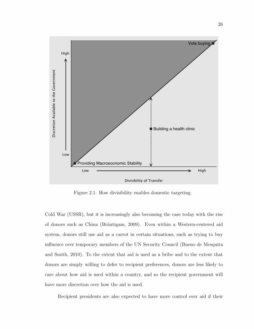
to recipient politicians. Figure 2.1 shows the divisibility of various goods. At the

bottom left corner is macroeconomic stability. It is a pure public good and is indi-

visible. Aid may encourage recipients to provide macroeconomic stability, but it is

impossible to selective allocate macroeconomy stability. At the top right of the figure

is vote buying. Besides being illegal, vote buying is targetable on an individual basis.

It enables an enormous amount of discretion. In between are a range of local public

goods. These goods operate like public goods but are bound to a specific geographic

area. Because they are bounded, politicians have the potential to aim these good at

some areas of the country and not at others. Foreign aid often provides local public

goods such as schools or roads.

Foreign aid can provide divisible, geographically bounded goods to voters. This

kind of transfer may remind some readers of clientelism. Clientelism is a transac-

tion between a politician and a citizen where a politician promises goods or services

in exchange for political support.9 Local public goods may be ripe for clientelistic

transfers, but there is an important di↵erence between the current work and much of

the work on clientelism. Clientelism is important in African studies because of the

bonds that it generates between a citizen and a politician. These bonds are often

built around the future expectations that each dyad has of the other.10 Politicians

pledge future material goods in exchange for political support in the present; voters

9For an overview of the concept of clientelism see Lemarchand and Legg (1972). For anoverview that specifically evaluates clientelism and ethnicity in Africa, see Lemarchand (1972).

10For example, Wantchekon (2003) tests the influence of clientelism using an experimentwhere some voters are promised closely targeted goods in the future.

25

pledge support in the future in exchange for goods now. This can be a rational

prospective strategy. Voters o↵er support in exchange for future benefits. The cur-

rent work models voters are retrospective. In this case, voters make decisions based

on their recent past and they generally do not attempt to isolate the source of the

improvement. In most cases, it is e↵ectively impossible for a voters to know if a

change in the level of goods and services that they experiences is due to donor or

recipient action. Further, this form of blind retrospection is common even in situ-

ations where voters might be expected to know that a politician is not responsible,

such as shark attacks (Achen and Bartels, 2004). In the words of one of the more

eloquent supporters of blind retrospection, “In order to ascertain whether the in-

cumbents have performed poorly or well, citizens need only calculate the changes

in their own welfare” (Fiorina, 1981, p. 5). Thus, the current work is more closely

aligned with clientelism not on the links between aid and voting, but on the idea

that politicians may try to strategically allocate aid. This use of clientelism draws

more on the idea that African governments tend to have power centralized around

the president. This centralization of power allows them strongly influence resource

distribution and this inevitably a↵ects the quality of electoral competition (van de

Walle, 2003). This centralization of power often allows presidents a large degree of

control over foreign as well as national resources.

Domestically, presidents will have more control over aid if they face fewer de

jure or de facto constraints on their exercise of power. Presidents will also have

more control over aid if donors are more willing to let recipients realize their own

preferences for the aid without donor interference. This was the case during the

Cold War, when donors were much more clearly using aid to secure international

political goals (Dunning, 2004). This factor will also be more likely to be present

if aid recipients have outside options for aid. Again, this was the case during the

26

Low High

Low

High

Divisibility of Transfer

Dis

cret

ion

Ava

ilabl

e to

the

Gov

ernm

ent

Providing Macroeconomic Stability

Vote buying

Building a health clinic

Figure 2.1. How divisibility enables domestic targeting.

Cold War (USSR), but it is increasingly also becoming the case today with the rise

of donors such as China (Brautigam, 2009). Even within a Western-centered aid

system, donors still use aid as a carrot in certain situations, such as trying to buy

influence over temporary members of the UN Security Council (Bueno de Mesquita

and Smith, 2010). To the extent that aid is used as a bribe and to the extent that

donors are simply willing to defer to recipient preferences, donors are less likely to

care about how aid is used within a country, and so the recipient government will

have more discretion over how the aid is used.

Recipient presidents are also expected to have more control over aid if their

27

governments are more involved in implementation. For example, aid could be chan-

neled through the recipient government or the recipient government could be an

integral part of the aid planning. If aid is channeled through NGOs or arms-length

organizations then the recipient government will be less able to exercise control over

the aid than if it was channeled through government bodies. If aid is given for

infrastructure that requires central planning, then the recipient will be heavily in-

volved in planning. While international donors can potentially have a great deal of

leeway in deciding where to build standalone buildings or where to provide one-o↵

services, they must cooperate with the government in the construction of networked

infrastructure like roads, piped water, or electric lines. This process will present the

recipient government with many points where they can influence the allocation of

resources. It is important to note that recipient control can be framed positively—as

an integral part of local country ownership—or negatively as opening the opportunity

for wasteful pork spending. For the current work, I am not interested in the long-run

implications of the degree of recipient discretion over aid allocations. Instead, I am

interested in the short-run implications of aid volatility and how that volatility is

translated into changes in distributions of resources that influence electoral outcomes

in recipient countries.

Aid recipients will have the least amount of control over aid if it is given around

the government to NGOs, then while it may still improve the lives of voters it will be

far less susceptible to influence by the recipient government. In one of the few tests

of the factors determining the allocation of NGO aid, it was shown that—at least

in Kenya—recipient government politicking does not influence NGO aid allocations

(Brass, 2011).11

11As Chapter 6 shows, this was clearly not the case for aid allocations the flowed through theKenyan government.

28

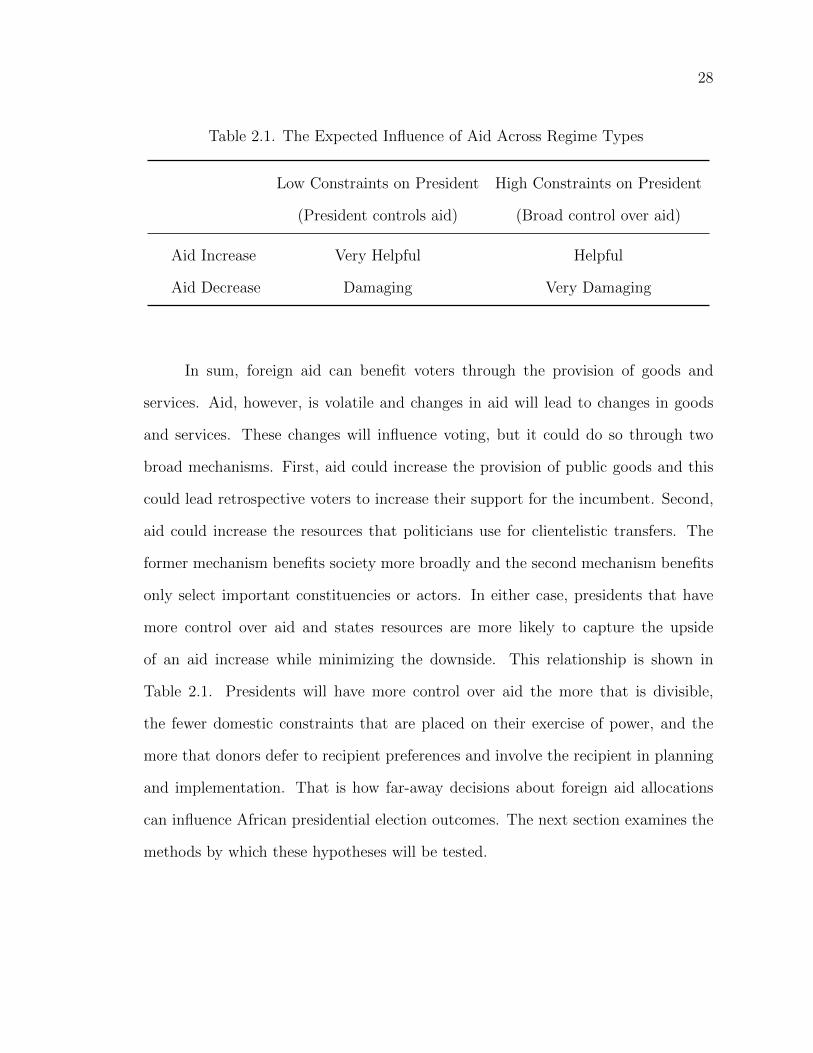
Table 2.1. The Expected Influence of Aid Across Regime Types

Low Constraints on President High Constraints on President

(President controls aid) (Broad control over aid)

Aid Increase Very Helpful Helpful

Aid Decrease Damaging Very Damaging

In sum, foreign aid can benefit voters through the provision of goods and

services. Aid, however, is volatile and changes in aid will lead to changes in goods

and services. These changes will influence voting, but it could do so through two

broad mechanisms. First, aid could increase the provision of public goods and this

could lead retrospective voters to increase their support for the incumbent. Second,

aid could increase the resources that politicians use for clientelistic transfers. The

former mechanism benefits society more broadly and the second mechanism benefits

only select important constituencies or actors. In either case, presidents that have

more control over aid and states resources are more likely to capture the upside

of an aid increase while minimizing the downside. This relationship is shown in

Table 2.1. Presidents will have more control over aid the more that is divisible,

the fewer domestic constraints that are placed on their exercise of power, and the

more that donors defer to recipient preferences and involve the recipient in planning

and implementation. That is how far-away decisions about foreign aid allocations

can influence African presidential election outcomes. The next section examines the

methods by which these hypotheses will be tested.

29

2.4 Methods

The rest of the dissertation investigates the claim that changes in foreign aid

influence election outcomes in recipient countries. The next chapter investigates the

claim that aid changes influence election results with a logistic regression using data

on over 100 presidential elections in Africa. Chapters 4, 5, and 6 trace out the causal

chains running from an aid fluctuation to vote changes in three individual elections.

To accomplish this task, I use process tracing. Process tracing is essentially a formal-

ized of more traditional qualitative or historical approaches to identifying causality

in single cases. Its defining features are its use of non-comparable observation to test

strong theoretical predictions about a causal process (George and Bennett, 2005;

Gerring, 2007). In all of the cases, it involves examining how changes in foreign aid

led to changes in the level of certain aid-funded goods and services and how these

changes in goods and services influenced voters. In Kenya and especially Malawi, it

also involves tracing a separate causal chains linking aid changes to changes in the

level of private resources available to politicians to private goods provided to voters.

The processes are generally examined at a fairly high level, usually at the level of

a sector or a small geographic unit such as a constituency. This approach shows in

detail how aid changes influenced the outcome of specific elections and allow us to

examine which mechanisms are connecting aid to votes. Before I discuss the details

of the methodology, I first discuss the scope conditions of my theory.

2.4.1 Scope Conditions

While the theory presented above may apply outside of Africa, this particular

analysis is bound geographically to sub-Saharan Africa and starts at the end of the

Cold War. The analysis is bound to Africa in attempt to limit confounding variables

and improve the validity of cross-country comparisons. Also, relative to a country’s

30

GDP or government budgets, foreign aid plays a larger role in Africa than in other

regions, which makes Africa a good place for a first test of my hypotheses. The

analysis starts at the end of the Cold War because the large structural shift from

bipolarity to unipolarity influenced the criteria that donors use to allocate aid to

Africa (Dunning, 2004).12 Finally, because this is a study of the e↵ect of aid on

election outcomes, I restrict the analysis to countries that held multiparty elections

in this time period. I am thus not testing for the e↵ect of aid on democratization,

only for the e↵ect of aid on incumbent advantage in countries that were already

holding elections.

2.4.2 Aid Changes Across Countries

When making a broad causal claim, it is useful to begin with a broad test

across all possible cases. For the claim of a link between aid changes and elec-

tion outcomes, this takes the form of a statistical analysis of the links between aid

changes and incumbent advantage in all African elections between 1990 and 2006.

This cross-national approach is most appropriate when the variables under analysis

are discrete and measurable and when there are a large number of fairly compa-

rable cases across which a covering law is expected to apply (King et al., 1994).

While this kind of a test often has trouble identifying a causal relationship, it is

still tremendously useful. After all, a correlation between aid changes and incum-

bent advantage is a necessary condition for a casual relationship. The details and

results of this analysis are presented in Chapter 3. It shows that there is in fact

a durable correlation between changes in aid going into the year before an election

and presidential incumbent advantage. While the large-n evidence is suggestive,

12Most African countries were not holding multiparty democratic elections before the end ofthe Cold War. The results of my regressions in Chapter 3 are unchanged by the inclusion of therelatively few multiparty African elections which occurred between 1969 and 1988.

31

cross-country regressions are notoriously unreliable because countries rarely satisfy

unit-homogeneity assumptions and the use of observational data means that there

are almost always reverse-causation and endogeneity concerns. While this evidence is

useful and supportive of the general argument, more detailed analyses are necessary

to demonstrate a plausible causal e↵ect of aid changes on election outcomes and to

show which mechanisms link the two variables.

2.4.3 Investigating Causality and Causal Mechanisms with Cases

Three case studies follow the cross-national regression. Two of these cases—

Ghana in 2000 and Malawi in 1999—were picked according to the regression residuals.

This case selection strategy follows the advice of Lieberman (2005), who recommends

selecting cases with small residuals if the goal of the case studies is to examine the

cases for causal mechanisms. With less jargon, this simply means that cases were

picked that were well predicted by the regression model. The specific cases are

discussed after the regressions, at the end of chapter 3.

Kenya’s 1992 election was also included, for three reasons. First, the Kenyan

case shows how an incumbent can respond to a planned, coordinated cut in aid from

all of its major donors. The cases of Ghana and Malawi show how governments

responded to completely unexpected changes in aid. In both of these cases neither

the donors or the recipients could have predicted that there would have been a large

change in aid flows. Kenya’s aid change was di↵erent, as it was driven by explicit

donor attempts to force an election, and so it may help to reveal if intentional donor

cuts have di↵erent e↵ects than unintentional ones. Second, Kenya in 1992 is probably

the most well known example of donors cutting aid in an attempt to force changes in

an aid recipient’s political institutions (Grosh and Orvis, 1996/97). In the Kenyan

case, Moi capitulated and held multiparty elections, but he then won those elections.

There is value in examining if the hypotheses proposed here hold in this well-known

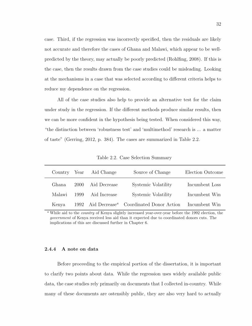
32

case. Third, if the regression was incorrectly specified, then the residuals are likely

not accurate and therefore the cases of Ghana and Malawi, which appear to be well-

predicted by the theory, may actually be poorly predicted (Rohlfing, 2008). If this is

the case, then the results drawn from the case studies could be misleading. Looking

at the mechanisms in a case that was selected according to di↵erent criteria helps to

reduce my dependence on the regression.

All of the case studies also help to provide an alternative test for the claim

under study in the regression. If the di↵erent methods produce similar results, then

we can be more confident in the hypothesis being tested. When considered this way,

“the distinction between ‘robustness test’ and ‘multimethod’ research is ... a matter

of taste” (Gerring, 2012, p. 384). The cases are summarized in Table 2.2.

Table 2.2. Case Selection Summary

Country Year Aid Change Source of Change Election Outcome

Ghana 2000 Aid Decrease Systemic Volatility Incumbent Loss

Malawi 1999 Aid Increase Systemic Volatility Incumbent Win

Kenya 1992 Aid Decreasea Coordinated Donor Action Incumbent Win

a While aid to the country of Kenya slightly increased year-over-year before the 1992 election, thegovernment of Kenya received less aid than it expected due to coordinated donors cuts. Theimplications of this are discussed further in Chapter 6.

2.4.4 A note on data

Before proceeding to the empirical portion of the dissertation, it is important

to clarify two points about data. While the regression uses widely available public

data, the case studies rely primarily on documents that I collected in-country. While

many of these documents are ostensibly public, they are also very hard to actually

33

locate and copy.13 The case studies rely primarily on government documents, NGO

reports, donor reports, interviews, and press clippings. Each of these sources has its

own biases, but I rely most heavily on government documents and press clippings

and these two documents have serious issues of bias.

The problem of bias arises because I typically have been unable to acquire a

full set of documents on whatever subject is under study. In the case of Ghana in

Chapter 4, I acquired a very good set of government data on electricity funding but I

was unable to locate a similar set of data for other local public goods such as roads.

In the case of Malawi, I located a powerful set of newspaper reports on corruption in

education, but I found nothing on corruption in other sectors such as the health. At

times I will be generalizing from these documents covering one sector or time period

to other sectors or time periods, and this requires that I carefully consider which way

the documents may be biased. While it is impossible to make precise statements on

the e↵ect of aid in one sector (where I do not have data) based on another sector

(where I have data), a knowledge of the direction bias can help reveal if a given

estimate is closer to the upper or lower bound of the true value. An awareness of the

direction of bias is thus immensely useful, and thankfully I believe that deducing it

is straightforward.

I believe that government documents will tend to under-report any activities

that the government does not want to be public knowledge. This is likely uncon-

tentious, but very useful. It means that if I use government documents and uncover

corruption or patterns of favouritism, then this is likely closer to the lower bound of

the true measure of such activities than it is to the upper bound. The opposite is true

of newspapers, which have an incentive to publish spectacular stories. In this case,

13In order to partially remedy this situation, and also to be more transparent in my research,I have been publishing these documents online at http://www.ryancbriggs.net/data.

34

the newspaper report probably reveals the upper bound of such activities.14 I will

use this argument in the case studies, when I am sometimes forced to make more

general claims about the extent of government discretion over aid or government

corruption from only a biased sample of data.

2.5 The plan for the remainder of the dissertation

The remainder of the dissertation is concerned with empirically testing the

claims above. The next chapter examines all African elections from 1990 until 2006

for evidence of an influence of aid changes on incumbent advantage. Chapters 4

through 6 examine specific instances of aid changes before elections. The case stud-

ies were picked specifically because they look like instances where aid may have

influenced election outcomes. By looking at these cases I hope to find evidence of

how aid changes influence voting patterns.15 The conclusion summarizes the previ-

ous empirical work, connects it back to the theory, and also interprets the results in

light of broad currents in the development literature. Finally, Appendix (A) presents

an agent-based model of donor decision making. This model shows that it is possible

to generate realistic levels of systemic aid volatility from plausible rules about donor

decision making.16 This helps to reinforce the dissertation’s claim that much of the

volatility in the aid system is due to uncoordinated, essentially random aid changes

on the part of donors.

14The case of newspapers is somewhat more di�cult than government documents, because alucky or skillful government can prevent newspapers from discovering corruption. However, it canbe uncontentiously said that estimates of corruption or favoritism that are drawn from governmentdocuments are much more likely to understate the problem than estimates drawn from press reports.

15Of course, not finding this evidence would also be important, because it would tell me thatmy regression is either misspecified or I am misinterpreting the results.

16More specifically, I can create realistic levels of systemic aid volatility from a model whereeach year a small random sample of donors make small, uncoordinated changes in their overall aidbudgets and disbursements.

35

CHAPTER 3

CROSS NATIONAL EVIDENCE

This chapter o↵ers the first empirical evidence for the claim that changes in

foreign aid influence incumbent advantage in Africa. Using a dataset of all African

elections after the Cold War, 1 it shows that fluctuations in aid in the year before an

election are related to changes in the odds of aid recipients winning elections. While

the data under study cannot speak directly to causation, the cross-national evidence

is broadly consistent with the hypotheses. The chapter also examines if di↵erent

kinds of countries respond di↵erently to aid changes. These results are mixed and

su↵er from gaps in important, relevant datasets. The chapter ends with a discussion

of case selection and a justification of the mechanisms under study in each case.

Before moving to the data, it is worth being clear about expectations. Aid

volatility in Africa is large and African voters claim to care about goods and services

that are very often aid-funded. There is also scattered evidence that African voters,

like voters elsewhere, often vote retrospectively based on their assessment of how

their life has changed under the recent rule of the incumbent. This means that aid

fluctuations are likely to translate into changes in the goods and services that voters

want, and therefore if aid declines before an election then incumbent will su↵er. If

aid rises, then incumbents should do better. This sort of broad pattern should be

1Dataset limitations prompted me to end the period under study in 2006.

36

evident in cross-national data.

3.1 Data

The key variables for this chapter are incumbent losses, and changes in the

level of foreign assistance. Election information, including information on incum-

bent losses, comes from a dataset maintained by Lindberg (2009). The dataset

includes information on all sub-Saharan African elections between 1990 and 2006.

I restricted my sample of elections to those where the incumbent, or someone from

the incumbent’s party or the incumbent’s chosen successor, contested the election.

The variable for ‘incumbent loss’ was constructed by amending Lindberg’s ‘turnover’

variable. In Lindberg’s dataset, presidential turnovers were marked with a 0 if there

was no turnover of power, 2 if there was a new president, and 1 if:

“the new person is an immediate successor to the old president for the sameparty [or] the new president is representing a new party but has served as aminister or similar in the old president’s regime” (Lindberg, 2006b).

For the purposes of this paper, a simple recoding of turnover into incumbent

loss would not be appropriate because, among other reasons, elections that the in-

cumbent did not contest always result in turnover and were coded ‘2’. I am interested

only in elections where the incumbent (or his party or his successor) contested, so

I examined each election that Lindberg coded 1 or 2 to see if the incumbent or the

incumbent’s party or immediate successor contested the election.2 After dropping

2There were nine elections where the incumbent (or party or successor) did not contest theelection, usually because the election was held after a coup or civil war. In the original dataset theseare marked as turnovers of power, as the leader before the election was di↵erent from the leaderafter the election. I have not included these elections because voters did not have the possibilityof voting for the incumbent, and the dissertation examines factors that influence if incumbentswin or lose. I also amended a number of elections where the incumbent lost to someone that waspreviously part of his party. I considered these as incumbent losses, while they are not consideredfull turnovers for Lindberg. Changes to the dataset are described in Tables 3.4 and 3.5 at the endof the Chapter.

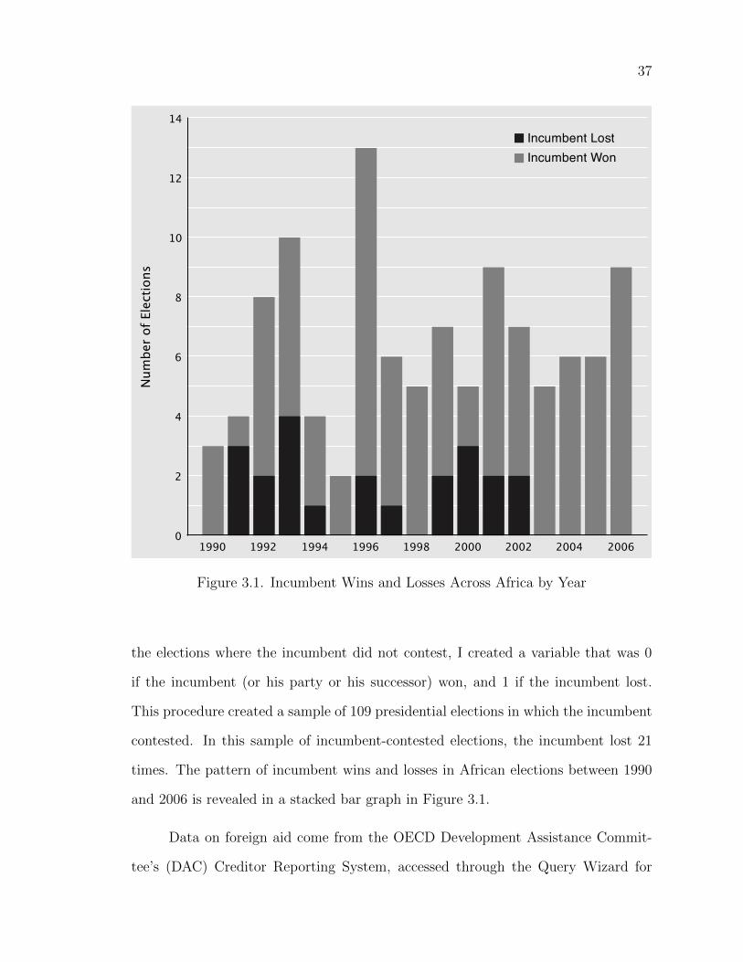
37

1990 1992 1994 1996 1998 2000 2002 2004 2006

14

0

2

4

6

8

10

12

Num

ber

of

Elec

tion

sIncumbent LostIncumbent Won

Figure 3.1. Incumbent Wins and Losses Across Africa by Year

the elections where the incumbent did not contest, I created a variable that was 0

if the incumbent (or his party or his successor) won, and 1 if the incumbent lost.

This procedure created a sample of 109 presidential elections in which the incumbent

contested. In this sample of incumbent-contested elections, the incumbent lost 21

times. The pattern of incumbent wins and losses in African elections between 1990

and 2006 is revealed in a stacked bar graph in Figure 3.1.

Data on foreign aid come from the OECD Development Assistance Commit-

tee’s (DAC) Creditor Reporting System, accessed through the Query Wizard for

38

International Development Statistics3 (Organization for Economic Co-operation and

Development, 2011). Aid is operationalized as net disbursements of Overseas De-

velopment Assistance (ODA) from all donors, less aid that was given for technical

cooperation or debt relief. This was done in order to only capture the portion of

aid that was capable of producing goods or services in a recipient country.4 Aid

is measured in millions of 2008 USD. Debt relief was excluded because it does not

represent a transfer of funds commensurate with the level of ODA that is reported

in the database. If debt is forgiven, then the recipient appears to receive the full

amount of debt as ODA, while in reality all that a government saves in the short-term

is the interest payment (that it may not have been paying). Funding for technical

cooperation goes primarily to consultants, and while perhaps valuable, a dollar of

technical assistance is not felt by voters in the same way as a dollar of project aid or

budget support. The DAC defines ODA as o�cial financial flows which are:

“administered with the promotion of the economic development and welfareof developing countries as the main objective, and which are concessional incharacter with a grant element of at least 25 percent (using a fixed 10 percentrate of discount)” (OECD, 2003).

ODA includes both bilateral flows and money that is given to multilateral

institutions if it will eventually meet the criteria described above. I examine how

an incumbent’s odds of reelection are a↵ected by changes in aid, so aid enters into

the analysis as changes in aid from the previous year. The key variable of interest

is the change in aid going into the year before the election. This was chosen for two

reasons. First, because elections are timed throughout the year and so aid changes

moving into an election year could potentially be responding to the outcome of the

3For my purposes this is a better dataset than AidData because while AidData includesinformation on aid from from NGOs, it only has data on commitments and not disbursements.

4Over the years in my sample, ODA with debt relief and technical cooperation removedcorrelates with regular ODA at r = 0.65. If I look only at ODA levels in election years then bothmeasures of aid correlate very highly (r = 0.96).

39

election rather than influencing them. Second, disbursed aid takes time to reach the

ground, and aid arriving at about the same time as an election does not have time

to influence the election’s outcome.

3.2 Initial Analysis

If aid changes are in fact influencing incumbent victory, then we should see

evidence of this in the cross-national data. Aid increases should show up more

frequently alongside incumbent victories and aid cuts should more frequently occur

before incumbent defeats. We can graphically examine the data to see if these

patterns exist.

Figure 3.2 shows the mean aid levels leading up elections across all of the elec-

tions in the sample. The elections are divided into one group that later experienced

an incumbent loss and one group that experienced an incumbent win. In times t-2

and t the aid levels between the two groups are indistinguishable at standard levels of

statistical significance. However, the aid levels at time t-1 are significantly di↵erent

and the change in levels is striking.5 The average winning incumbent received over

100 million 2008 USD more in aid than the average losing incumbent. Further, there

is a clear pattern where average aid levels increase in the case of victories and aid

decrease in the cases of losses.

The graph shows clearly that incumbents that lose and incumbents that win

tend to see di↵erent patterns in aid flows before their respective elections. However,

figure 3.2 does not tell us if the magnitude of the aid change has any e↵ect on the

likelihood of an incumbent winning or losing. To investigate this relationship, it is

more useful to divide the groups by the size and direction of the aid cut and not by

5A one-tailed t-test (unequal variance) yields p=.017. The p values comparing aid levels attimes t-2 and t are 0.479 and 0.309, respectively.

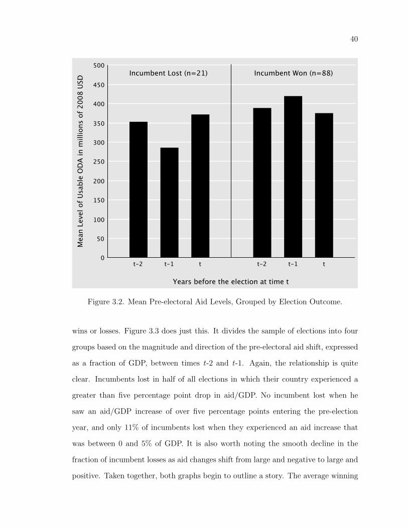
40

t-2 t-1 t t-2 t-1 t

500

0

50

100

150

200

250

300

350

400

450

Years before the election at time t

Mea

n Le

vel o

f Usa

ble

OD

A in

mill

ions

of 2

008

USD

Incumbent Lost (n=21) Incumbent Won (n=88)

Figure 3.2. Mean Pre-electoral Aid Levels, Grouped by Election Outcome.

wins or losses. Figure 3.3 does just this. It divides the sample of elections into four

groups based on the magnitude and direction of the pre-electoral aid shift, expressed

as a fraction of GDP, between times t-2 and t-1. Again, the relationship is quite

clear. Incumbents lost in half of all elections in which their country experienced a

greater than five percentage point drop in aid/GDP. No incumbent lost when he

saw an aid/GDP increase of over five percentage points entering the pre-election

year, and only 11% of incumbents lost when they experienced an aid increase that

was between 0 and 5% of GDP. It is also worth noting the smooth decline in the

fraction of incumbent losses as aid changes shift from large and negative to large and

positive. Taken together, both graphs begin to outline a story. The average winning

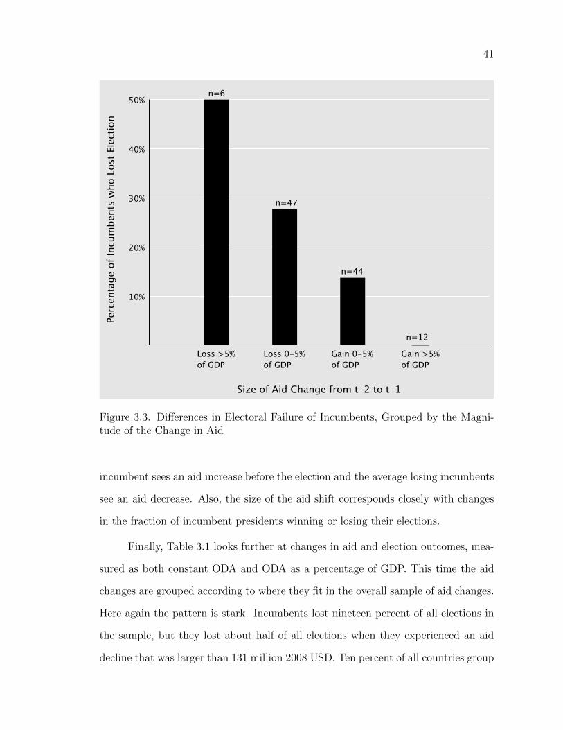
41

Loss >5%of GDP

Loss 0-5%of GDP

Gain 0-5%of GDP

Gain >5%of GDP

50%

10%

20%

30%

40%

Size of Aid Change from t-2 to t-1

Perc

enta

ge o

f In

cum

ben

ts w

ho L

ost

Elec

tion

n=6

n=47

n=44

n=12

Figure 3.3. Di↵erences in Electoral Failure of Incumbents, Grouped by the Magni-tude of the Change in Aid

incumbent sees an aid increase before the election and the average losing incumbents

see an aid decrease. Also, the size of the aid shift corresponds closely with changes

in the fraction of incumbent presidents winning or losing their elections.

Finally, Table 3.1 looks further at changes in aid and election outcomes, mea-

sured as both constant ODA and ODA as a percentage of GDP. This time the aid

changes are grouped according to where they fit in the overall sample of aid changes.

Here again the pattern is stark. Incumbents lost nineteen percent of all elections in

the sample, but they lost about half of all elections when they experienced an aid

decline that was larger than 131 million 2008 USD. Ten percent of all countries group

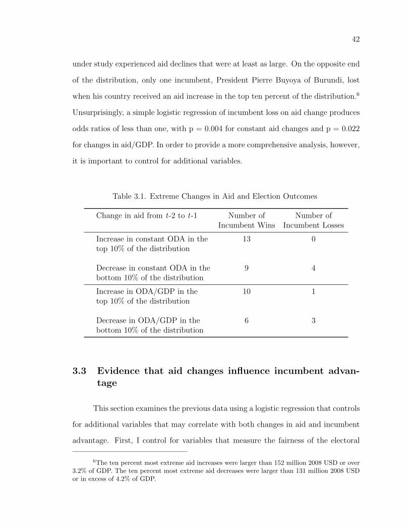
42

under study experienced aid declines that were at least as large. On the opposite end

of the distribution, only one incumbent, President Pierre Buyoya of Burundi, lost

when his country received an aid increase in the top ten percent of the distribution.6

Unsurprisingly, a simple logistic regression of incumbent loss on aid change produces

odds ratios of less than one, with p = 0.004 for constant aid changes and p = 0.022

for changes in aid/GDP. In order to provide a more comprehensive analysis, however,

it is important to control for additional variables.

Table 3.1. Extreme Changes in Aid and Election Outcomes

Change in aid from t-2 to t-1 Number of Number ofIncumbent Wins Incumbent Losses

Increase in constant ODA in the 13 0top 10% of the distribution

Decrease in constant ODA in the 9 4bottom 10% of the distribution

Increase in ODA/GDP in the 10 1top 10% of the distribution

Decrease in ODA/GDP in the 6 3bottom 10% of the distribution

3.3 Evidence that aid changes influence incumbent advan-tage

This section examines the previous data using a logistic regression that controls

for additional variables that may correlate with both changes in aid and incumbent

advantage. First, I control for variables that measure the fairness of the electoral

6The ten percent most extreme aid increases were larger than 152 million 2008 USD or over3.2% of GDP. The ten percent most extreme aid decreases were larger than 131 million 2008 USDor in excess of 4.2% of GDP.

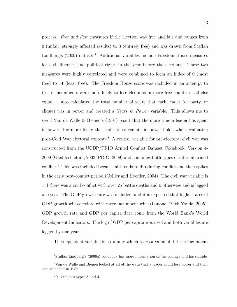
43

process. Free and Fair measures if the election was free and fair and ranges from

0 (unfair, strongly a↵ected results) to 3 (entirely free) and was drawn from Sta↵an

Lindberg’s (2009) dataset.7 Additional variables include Freedom House measures

for civil liberties and political rights in the year before the elections. These two

measures were highly correlated and were combined to form an index of 0 (most

free) to 14 (least free). The Freedom House score was included in an attempt to

test if incumbents were more likely to lose elections in more free countries, all else

equal. I also calculated the total number of years that each leader (or party, or

clique) was in power and created a Years in Power variable. This allows me to

see if Van de Walle & Bienen’s (1991) result that the more time a leader has spent

in power, the more likely the leader is to remain in power holds when evaluating

post-Cold War electoral contests.8 A control variable for pre-electoral civil war was

constructed from the UCDP/PRIO Armed Conflict Dataset Codebook, Version 4-

2009 (Gleditsch et al., 2002; PRIO, 2009) and combines both types of internal armed

conflict.9 This was included because aid tends to dip during conflict and then spikes

in the early post-conflict period (Collier and Hoe✏er, 2004). The civil war variable is

1 if there was a civil conflict with over 25 battle deaths and 0 otherwise and is lagged

one year. The GDP growth rate was included, and it is expected that higher rates of

GDP growth will correlate with more incumbent wins (Lanoue, 1994; Youde, 2005).

GDP growth rate and GDP per capita data come from the World Bank’s World

Development Indicators. The log of GDP per capita was used and both variables are

lagged by one year.

The dependent variable is a dummy which takes a value of 0 if the incumbent

7Sta↵an Lindberg’s (2006a) codebook has more information on his codings and his sample.

8Van de Walle and Bienen looked at all of the ways that a leader could lose power and theirsample ended in 1987.

9It combines types 3 and 4.

44

wins and 1 if the incumbent loses, so a logistic regression is estimated. Robust

standard errors are clustered by country. Additionally, binary dependent variables

with panel data are likely to violate the assumption of independence of observations

required for ordinary logistic analysis (Beck et al., 1998). Unfortunately, I have

too few observations (elections) per country to use Beck, Katz, and Tucker’s (1998)

preferred approach. Following Susan Hyde (2011), I add a variable which measures

the number of previous incumbent losses in each country. I also add a year variable

to catch any remaining time trends.10 The latter is especially important because

Figure 3.1 shows that incumbent losses have generally declined during the period

under study.

I ran three regressions. Regression one operationalized aid change as the change

in constant ODA between times t-2 and t-1, where time t is the year of the election.

Regression two operationalized aid change as a fraction of GDP and regression three

operationalized it on a per capita basis. Aside from the di↵erent aid variables, the

regressions are similar. The initial regression results may be driven by outliers and

should be viewed skeptically. They are included at the end of the Chapter in Table

3.6. To generate more reliable results I predict probabilities of turnover using these

full-sample regressions and then graphed the predicted probability of turnover against

aid changes.11 This is shown in Figure 3.4. There are lines marking the -400 and

+400 points on the x-axis. These lines separate 7 outlying observations from the rest

of the distribution.

I reran regression 1 while dropping observations with aid changes that were

10Time trends are removed from the aid variable because I evaluate the e↵ect of aid changes

on incumbent advantage. Creating the aid change variable requires first di↵erencing. Incumbentloss is a binary variable and is dealt with similar to Hyde (2011).

11All I actually needed to see outliers is to evaluate the spread of aid changes, but the extrainformation from the predicted probabilities helps to show if the outliers correspond with very largeor small expected values of turnover.

45

0.2

.4.6

.81

Pr(inc_loss)

-500 0 500 1000 1500Useable_ODA_t2_t1

Figure 3.4. Outliers in the Aid Change variable

larger than 400 million ODA in either direction.12 The results do not change sig-

nificantly, though the p-values for the aid change variables increase slightly. I then

predicted new probabilities of turnover from the outlier-free version of regression 1

and then recreated Figure 3.4 using the new bounds of ODA change. This is shown

in Figure 3.5, which is accompanied by a best fit line showing the relationship be-

tween the newly predicted probability of turnover and the outlier-free sample of aid

changes.

I followed the same general approach for all three specifications (raw aid

change, aid change measured as a fraction of GDP, and the change in aid per capita).

12Adding dummy variables for similarly large changes in either direction and including theobservations produces similar results.

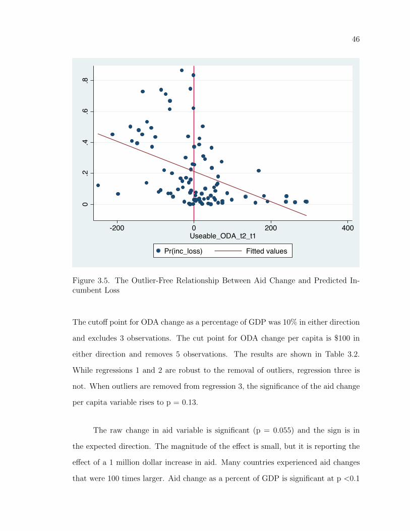
46

0.2

.4.6

.8

-200 0 200 400Useable_ODA_t2_t1

Pr(inc_loss) Fitted values

Figure 3.5. The Outlier-Free Relationship Between Aid Change and Predicted In-cumbent Loss

The cuto↵ point for ODA change as a percentage of GDP was 10% in either direction

and excludes 3 observations. The cut point for ODA change per capita is $100 in

either direction and removes 5 observations. The results are shown in Table 3.2.

While regressions 1 and 2 are robust to the removal of outliers, regression three is

not. When outliers are removed from regression 3, the significance of the aid change

per capita variable rises to p = 0.13.

The raw change in aid variable is significant (p = 0.055) and the sign is in

the expected direction. The magnitude of the e↵ect is small, but it is reporting the

e↵ect of a 1 million dollar increase in aid. Many countries experienced aid changes

that were 100 times larger. Aid change as a percent of GDP is significant at p <0.1

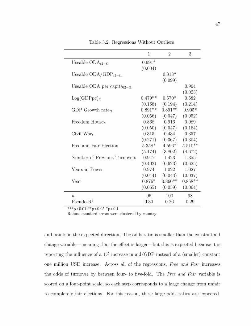
47

Table 3.2. Regressions Without Outliers

1 2 3

Useable ODAt2�t1 0.991*(0.004)

Useable ODA/GDPt2�t1 0.818*(0.099)

Useable ODA per capitat2�t1 0.964(0.023)

Log(GDPpc)t1 0.479** 0.570* 0.582(0.168) (0.194) (0.214)

GDP Growth ratet1 0.891** 0.891** 0.905*(0.056) (0.047) (0.052)

Freedom Houset1 0.868 0.916 0.989(0.050) (0.047) (0.164)

Civil Wart1 0.315 0.434 0.357(0.271) (0.367) (0.304)

Free and Fair Election 5.358* 4.596* 5.510**(5.174) (3.802) (4.672)

Number of Previous Turnovers 0.947 1.423 1.355(0.402) (0.623) (0.625)

Years in Power 0.974 1.022 1.027(0.044) (0.043) (0.037)

Year 0.876* 0.860** 0.858**(0.065) (0.059) (0.064)

n 96 100 98Pseudo-R2 0.30 0.26 0.29

***p<0.01 **p<0.05 *p<0.1Robust standard errors were clustered by country

and points in the expected direction. The odds ratio is smaller than the constant aid

change variable—meaning that the e↵ect is larger—but this is expected because it is

reporting the influence of a 1% increase in aid/GDP instead of a (smaller) constant

one million USD increase. Across all of the regressions, Free and Fair increases

the odds of turnover by between four- to five-fold. The Free and Fair variable is

scored on a four-point scale, so each step corresponds to a large change from unfair

to completely fair elections. For this reason, these large odds ratios are expected.

48

Incumbents are more likely to lose elections that are fair. Countries that experience

GDP growth before the election are less likely to experience turnover and the result

is fairly large. Turnover is also less likely in richer countries. Finally, even after

controlling for the other variables, time still matters. Turnover is less likely as time

goes on.

One potential problem is that these results may be driven by reverse-causation

and are prone to endogeneity problems. The best solution to this is to find an

instrument for aid changes and then run a two-stage least-squares regression. Un-

fortunately, while a number of instruments for aid levels have been proposed, these

either are not sensitive to annual changes in aid (this includes instruments such as

colonial origin dummies, infant mortality at an earlier time period or initial GDP

per capita) or do not meet the exclusion restriction and/or do not capture a repre-

sentative slice of aid disbursements. For example, while the the log of donor GDP

combined with a score measuring ‘a�nity with America’ (UN vote share in common)

may capture a sample of foreign aid that is essentially random in relation to conflict

onset (Savun and Tirone, 2011), this is not likely to be the case with a dependent

variable measuring election outcomes (Faye and Niehaus, 2010). While the lack of an

instrument should increase our skepticism in the findings, I remain doubtful that the

results are driven by endogeneity for a few reasons. First, the most recent study of aid

volatility noted that for both total ODA and my measure of useable aid, “electoral

cycles or movements along a political spectrum due to governmental changes does

not a↵ect volatility” (Kharas and Desai, 2010, p. 19).13 The same study noted that

“all in all, there are relatively few recipient-country traits that influence volatility in

a consistent manner” (Kharas and Desai, 2010, p. 24). Second, reverse causation

13The authors created a measure of aid that looked at net ODA and ignored technical as-sistance and debt relief, making it very similar or possibly identical to my measure of ‘useableODA.’

49

would require donors to correctly guess election outcomes years in advance and then

be able to quickly change aid allocations in response to their guesses. Additionally,

to match the results above, donors would also have to stop favouring likely-to-win

incumbents in the year going into the election, as the variables for the period from

the year before the election to the election year were insignificant.14 This all seems

very unlikely, and by far the simplest explanation for the patterns in Table 3.2 is

that aid increases directly help incumbents win elections and aid decreases hurt their

chances. The next section uses the outlier-free regressions above and examines if the

results are being driven by multicollinearity. It also tests to ensure that the results

are robust to small changes in the specification.

3.4 Multicollinearity and Sensitivity Tests

This section examines the sensitivity of regressions 1 and 2 in Table 3.2 to

minor changes to the specification and to multicollinearity. Specifically, it drops

variables with very low tolerances (which implies that they are highly collinear to

the other independent variables).15 When I examine the tolerance of the indepen-

dent variables after running the outlier-free version of regression 1, I produced some

potentially troubling results. The tolerance for the year variable, for example, is a

tiny 0.008. The second smallest tolerance is the log of GDP per capita, which is 0.02.

Starting from the lowest tolerance levels, I sequentially drop any variable that has a

tolerance below 0.1. This generally lowers the p-values of the remaining variables by

a small amount, strengthening the results, but does not change the main findings.

The same is true when I sequentially drop low-tolerance variables from regression 2.

Other variables become slightly more significant, but the substantive findings remain

14This is explained further in section 3.4.

15For a longer discussion of tolerances and variance inflation factors, including a cautionagainst overly relying on simple rules for interpreting variance inflation factors, see O’Brien (2007).

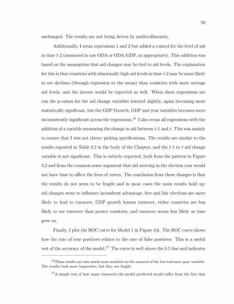
50

unchanged. The results are not being driven by multicollinearity.

Additionally, I reran regressions 1 and 2 but added a control for the level of aid

in time t-2 (measured in raw ODA or ODA/GDP, as appropriate). This addition was

based on the assumption that aid changes may be tied to aid levels. The explanation

for this is that countries with abnormally high aid levels in time t-2 may be more likely

to see declines (through regression to the mean) than countries with more average

aid levels, and the inverse would be expected as well. When these regressions are

run the p-values for the aid change variables lowered slightly, again becoming more

statistically significant, but the GDP Growth, GDP and year variables becomes more

inconsistently significant across the regressions.16 I also reran all regressions with the

addition of a variable measuring the change in aid between t-1 and t. This was mainly

to ensure that I was not cherry picking specifications. The results are similar to the

results reported in Table 3.2 in the body of the Chapter, and the t-1 to t aid change

variable is not significant. This is entirely expected, both from the pattern in Figure

3.2 and from the common sense argument that aid arriving in the election year would

not have time to a↵ect the lives of voters. The conclusion from these changes is that

the results do not seem to be fragile and in most cases the main results hold up:

aid changes seem to influence incumbent advantage, free and fair elections are more

likely to lead to turnover, GDP growth lessens turnover, richer countries are less

likely to see turnover than poorer countries, and turnover seems less likely as time

goes on.

Finally, I plot the ROC curve for Model 1 in Figure 3.6. The ROC curve shows

how the rate of true positives relates to the rate of false positives. This is a useful

test of the accuracy of the model.17 The curve is well above the 0.5 line and indicates

16These results are also much more sensitive to the removal of the low-tolerance year variable.The results look more impressive, but they are fragile.

17A simple test of how many turnovers the model predicted would su↵er from the fact that

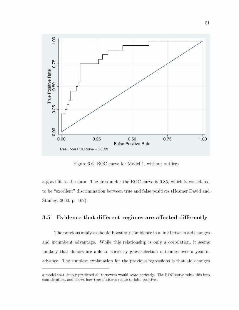
51

0.00

0.25

0.50

0.75

1.00

True

Pos

itive

Rate

0.00 0.25 0.50 0.75 1.00False Positive Rate

Area under ROC curve = 0.8533

Figure 3.6. ROC curve for Model 1, without outliers

a good fit to the data. The area under the ROC curve is 0.85, which is considered

to be “excellent” discrimination between true and false positives (Hosmer David and

Stanley, 2000, p. 162).

3.5 Evidence that di↵erent regimes are a↵ected di↵erently

The previous analysis should boost our confidence in a link between aid changes

and incumbent advantage. While this relationship is only a correlation, it seems

unlikely that donors are able to correctly guess election outcomes over a year in

advance. The simplest explanation for the previous regressions is that aid changes

a model that simply predicted all turnovers would score perfectly. The ROC curve takes this intoconsideration, and shows how true positives relate to false positives.

52

can influence the odds of an incumbent winning re-election. However, that was only

the first hypothesis.

The second part of the theory explained that presidents in some kinds of coun-

tries should electorally benefit more from aid changes than presidents in others. This

section examines the cross-national evidence to see if it supports this claim. In order

to test the idea that presidents in di↵erent countries are a↵ected di↵erently by aid

changes, I constructed dummy variables which corresponded to a better quality of

government and a more mature democracy. I then re-ran regressions 1 and 2 but

included the dummy variable and an interaction term between the dummy variable

and the main aid change variable. This allows me to separately test for the influence

of aid changes in the groups of countries divided by the dummy variable.18

Quality of Government Interactions

The first dummy variable was aimed at measuring the quality of government.

This was constructed using the International Country Risk Guide’s (ICRG) mea-

sures of Bureaucratic Quality and Corruption, which were both measured from 1–6

and were combined into a 12-point index.19 The ICRG is constructed by Political

Risk Services Group, a private company, and has been used primarily in economics

research for at least 15 years.20

The ICRG measure of Bureaucratic Quality aims at capturing the degree to

which bureaucracies are competent and free from direct political influence. Higher

scores are given to countries with a higher quality bureaucracy. The corruption

18For a refresher on how this works and why this is the case, see Braumoeller (2004).

19Between 1997 and 1998 the ICRG rescaled their measure of bureaucratic quality from a0–6 scale to a 0–4 scale, so I multiplied all values after 1997 by 1.5. This modification of the ICRGdata was done before by Knack and Rahman (2007).

20For a small sample of articles using the ICRG, see Acemoglu et al. (2001); Charron andLapuente (2011); Knack (1996, 2001).

53

score aims at measuring “actual or potential corruption in the form of excessive

patronage, nepotism, job reservations, ‘favor-for-favors’, secret party funding, and

suspiciously close ties between politics and business” (Political Risk Services, 2011).

It secondarily tries to capture petty corruption. Higher scores are given to countries

with less corruption.21 This index has a maximum score of 12, which would be given

to countries that had very little corruption and a very high quality bureaucracy. The

average score in my total sample was 4.1 and the average of the election-years in my

sample was 4.3. These are essentially the same score because the index is scored in

half-point increments. I created a dummy variable, QoGdummy, which takes a score

of 0 if the QoG score is less than 4.3 and 1 if it is above 4.3. Therefore, QoGdummy

has a value of 1 in the better governed countries. I then interacted this dummy

variable with the aid change variables in regressions 1 and 2 from Table 3.2. I reran

the regressions with both lower-order terms and the interaction term.

The ICRG interaction-term regressions (not shown) are inconclusive. More

specifically, nothing is significant. The problem isn’t the interaction term,22 the

problem is the contraction in sample size. While the ICRG index is the most com-

prehensive dataset in its class, it still has large gaps in Africa. Using the ICRG

index lowers the number of observations in my sample from 109 to 65.23 The fact

that sample size is the problem can be easily shown by running regressions 1 and 2

from Table 3.2 with the ICRG sample of 65 elections, but no ICRG variables. Again,

all of the key variables drop in significance to the point where nothing has a p-value

below 0.1. The ICRG interaction regressions are very likely underpowered and no

21For more information on the ICRG methodology Political Risk Services (2011).

22I tried using di↵erent cut points in the construction of the dummy variable and di↵erentways of combining the QoG variable with the aid term. It just doesn’t work.

23Additionally, the ICRG is created by a private company that sells their data, therefore itis likely that their selection of countries to cover is not random. This means that there is likelyselection bias in the selection of countries and that will now a↵ect the results.

54

variables are significant. Without other sources of data, this approach is fruitless.

Two Turnover Interactions

I also created a variable that measured if the democracy was better established.

My measure for an established democracy is based on the idea of the two-turnover

test (Huntington, 1991). I created a variable which is 1 if the country has experienced

two or more elections where the incumbent lost and 0 otherwise.24 While this measure

is admittedly crude, it should capture the idea that some democracies have more of

a history with turnover than others. While less precise, this variable also does not

cause the sample size to contract by one-third. Regressions 1 and 2 in Table 3.7

at the end of the Chapter show the interactions of two turnover with aid change,

measured as raw ODA or a fraction of GDP. Here the evidence for heterogeneity

across types of countries fares better, but the results are problematic.

In general, the results look good. In both regressions the lower-order aid

change variable is significant and the interaction term is not. Due to the nature

of interaction terms, this tells us that the aid change variable is significant when

two turnover is 0 and insignificant in the countries that have experienced at least

two instances of incumbent electoral losses. This means that presidents are better

helped by aid in the countries that have less experience with turnover and are not

significantly influenced by aid in the countries with more of a history of turnover.

The Free and Fair variable also increases slightly in regression 1 to p=0.108, but I

don’t consider this to be a major problem. The larger problem is that most countries

haven’t experienced two elections in which the incumbent lost. In fact, two turnover

is only positive for 7 observations and 5 countries: Benin, Cape Verde, the Central

African Republic, Madagascar, and Niger. This sparse coverage should cause us to

24The variable is by no means a perfect reflection of Huntington’s original concept. It doesnot reset in the case of a coup or other break with democracy, for example.

55

dramatically downplay how seriously we take the results. Even if this variable is

getting at some measure of democratic consolidation (and it may not be), too few

countries in Africa have experienced two turnovers to make the variable reliable.

Again, data problems prevent me from probing this further. There simply haven’t

been enough elections to untangle this pattern with a large-n study of this kind.

3.6 Picking cases

The natural solution to these data availability problems is to rely more strongly

on a deep analysis of case studies. In this section I pick cases with the aid of the

residuals from the regressions. The cases need to meet a few criteria. First, they

should be reasonably well predicted by the regressions. Second, their aid changes

should be fairly large. Some cases will be well predicted by the regressions purely

due to the presence of control variables. This over-inclusion of controls is something

that Lieberman (2005) cautions against. This is potentially an issue because it will

lead to well predicted cases with only small aid changes. As such, I also construct a

stripped down “case-selection regression” model and take its predicted probabilities

of turnover into account as well. Third, I want one case of aid increases and one case

of aid decreases. Fourth, I intentionally want to select cases that look like they will

fit the first hypothesis so that I can examine them for mechanisms.25 This means

that I need to select one case of turnover after aid declined and one case of incumbent

victory after aid increased.

25This point can be easily misunderstood. The goal here is to pick cases where the twoendpoints—aid change in the year before the election and an election result—match the theory.The empirical work then tests for ways that the change in aid could have influenced the electionresults.

56

3.6.1 Ghana, 2000

Ghana in 2000 is an obvious choice. The country saw an aid decline of about

between 1–2% of GDP before its election and the incumbent lost. About half of this

decline was from the IDA and the rest was spread across many donors. This makes

it fairly likely that the decline was not due to some intentional aid reduction but

rather the result of poor donor coordination. I generated predict probabilities from

Regression 1 in Table 3.2 and Ghana’s predicted probability of turnover is in the top

quarter of all elections. All of this makes Ghana in 2000 an excellent case.

3.6.2 Malawi, 1999

Malawi in 1999 is slightly more mixed. There are distinct advantages to picking

Malawi. First it saw a large aid increase in the year before the election. The aid

increase came to about 5% of GDP. Also, like Ghana, about half of the aid change

was due to one donor (the EC) and the other half was due to small changes on the

part of other donors. Regression 1 gave Malawi a predicted probability of turnover

that was 0.22, which is fairly close to its actual value of 0 (there was no turnover in

the 1999 election). This looks like a decent match, but many countries have scores

well under 0.22.26 To see how much of this was being driven by control variables,

I reran regression 1 from Table 3.2 but I dropped everything but the aid change

variable and the year (I still wanted to control for a time trend). The variables

were strongly significant and I used this to predict probabilities of turnover. Now

Malawi’s predicted probability of turnover is 0.07 and the mean across all elections

in the sample is 0.20.27 Malawi’s large aid change from a diverse number of donors,

26Based on control variables, Kenya in 1992 scored 0.09, meaning that Moi’s victory is reallynot surprising from the point of view of the general regression model.

27Ghana’s predicted probability of turnover is still well above the mean of the predictedprobabilities in this stripped-down regression. Also, dropping many of the control variables mayintroduce bias in the estimation of the e↵ect of aid, and thus the predicted probabilities of turnover.

57

its fit within the demands of what I need in a positive case, and its generally good

predicted probabilities make it a good selection.

3.6.3 Kenya, 1992

Kenya was not selected according to the regression results. It was instead se-

lected for two other reasons. First, it was selected because the Kenyan aid cut in

1991 is the most well known case of an aid reduction that is obviously endogenous

to a recipient election.28 Second, Kenya at this time was lead by a president with

a very high degree of domestic discretion. The Kenyan case can thus help to exam-

ine if discretion helps to blunt the e↵ects of an aid cut, as proposed in Table 2.1.

Finally, any selection strategy that is independent of the regression o↵ers more new

information to test the theory that aid changes influence incumbent advantage.

3.6.4 Case Selection Summary

Every case study examines the mechanisms linking an aid increase or decrease

to incumbent advantage, but the specific manifestations of the mechanism (roads,

education) change from case to case. The choice to study a specific sector matters

greatly, because there is evidence that di↵erent sectors within the same countries

are often targeted according to distinct political logics (Posner and Kramon, 2011).

My selection strategy is straightforward. In every chapter, I examined the electoral

distribution and electoral e↵ects of aid to the sector that were impacted by the

change in aid. Ghana’s Ministry of Energy experienced a decline in developmental

The advice from Lieberman (2005) is that this should be kept in mind but that the case studiescan also help to show when and where control variables are necessary. I am skeptical of this pointbecause dropping control variables can lead to biased case selection and it is not clear how casestudy analysis of biased cases will lead to a better sense of which control variables are important inthe regression specification. I still feel that this factor is useful so long as it is interpreted alongsidethe other factors influencing case selection.

28Interestingly, while the Kenyan government experienced a large decline in aid, the countrysaw year-over-year increases in aid from 1990 until 1993.

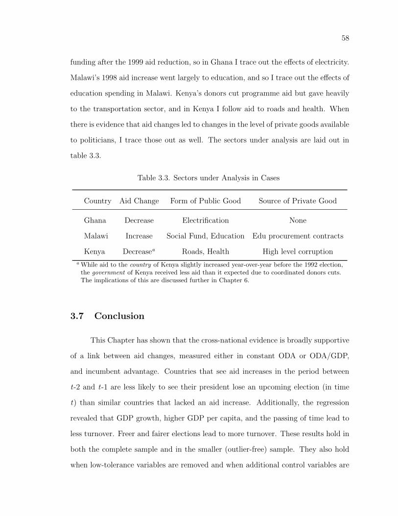
58

funding after the 1999 aid reduction, so in Ghana I trace out the e↵ects of electricity.

Malawi’s 1998 aid increase went largely to education, and so I trace out the e↵ects of

education spending in Malawi. Kenya’s donors cut programme aid but gave heavily

to the transportation sector, and in Kenya I follow aid to roads and health. When

there is evidence that aid changes led to changes in the level of private goods available

to politicians, I trace those out as well. The sectors under analysis are laid out in

table 3.3.

Table 3.3. Sectors under Analysis in Cases

Country Aid Change Form of Public Good Source of Private Good

Ghana Decrease Electrification None

Malawi Increase Social Fund, Education Edu procurement contracts

Kenya Decreasea Roads, Health High level corruption

a While aid to the country of Kenya slightly increased year-over-year before the 1992 election,the government of Kenya received less aid than it expected due to coordinated donors cuts.The implications of this are discussed further in Chapter 6.

3.7 Conclusion

This Chapter has shown that the cross-national evidence is broadly supportive

of a link between aid changes, measured either in constant ODA or ODA/GDP,

and incumbent advantage. Countries that see aid increases in the period between

t-2 and t-1 are less likely to see their president lose an upcoming election (in time

t) than similar countries that lacked an aid increase. Additionally, the regression

revealed that GDP growth, higher GDP per capita, and the passing of time lead to

less turnover. Freer and fairer elections lead to more turnover. These results hold in

both the complete sample and in the smaller (outlier-free) sample. They also hold

when low-tolerance variables are removed and when additional control variables are

59

added to the regression. This evidence is supportive of the main hypothesis that aid

increases help incumbents and aid decreases hurt them.

The cross-national evidence can say much less about the idea that di↵erent

regimes are a↵ected di↵erently by aid changes. The ICRG data does not have suf-

ficient coverage in Africa to provide useful results. The two-turnover variable looks

more promising, but not enough countries have experienced turnover for it to be

reliable. This means that while the cross-national evidence is supportive of the main

hypothesis, the case studies must be relied upon more heavily for testing the various

mechanisms linking aid changes to election outcomes. Specifically, they can help to

reveal when foreign aid influences election outcomes through public or private goods

mechanisms. They can also help to show how if foreign aid is allocated according to

a political logic and the form of that logic (targeting core or swing voters). The next

chapter presents the case of Ghana’s election in 2000.

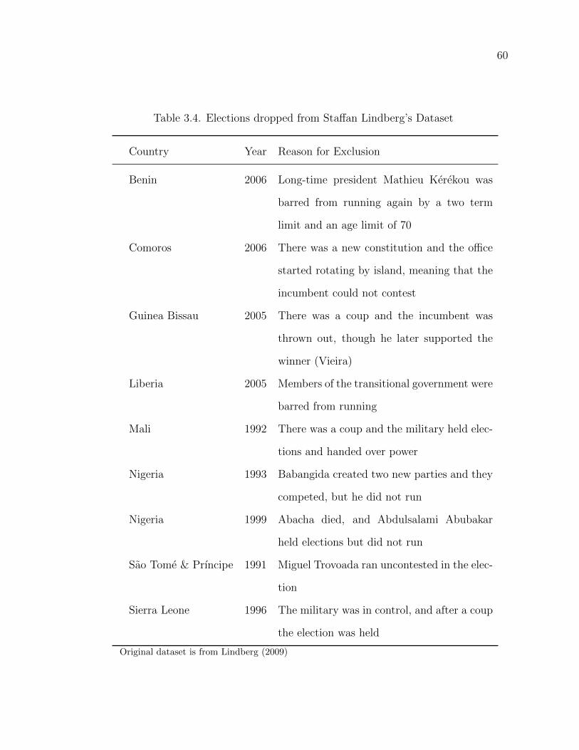
60

Table 3.4. Elections dropped from Sta↵an Lindberg’s Dataset

Country Year Reason for Exclusion

Benin 2006 Long-time president Mathieu Kerekou was

barred from running again by a two term

limit and an age limit of 70

Comoros 2006 There was a new constitution and the o�ce

started rotating by island, meaning that the

incumbent could not contest

Guinea Bissau 2005 There was a coup and the incumbent was

thrown out, though he later supported the

winner (Vieira)

Liberia 2005 Members of the transitional government were

barred from running

Mali 1992 There was a coup and the military held elec-

tions and handed over power

Nigeria 1993 Babangida created two new parties and they

competed, but he did not run

Nigeria 1999 Abacha died, and Abdulsalami Abubakar

held elections but did not run

Sao Tome & Prıncipe 1991 Miguel Trovoada ran uncontested in the elec-

tion

Sierra Leone 1996 The military was in control, and after a coup

the election was held

Original dataset is from Lindberg (2009)

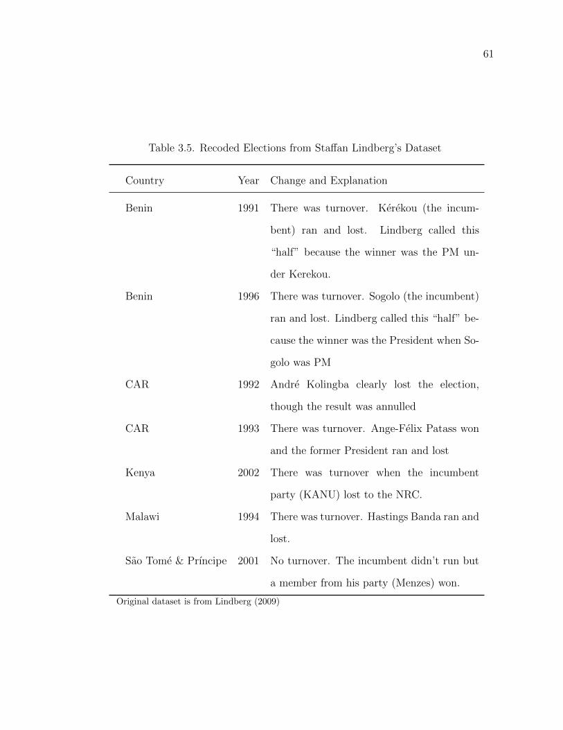
61

Table 3.5. Recoded Elections from Sta↵an Lindberg’s Dataset

Country Year Change and Explanation

Benin 1991 There was turnover. Kerekou (the incum-

bent) ran and lost. Lindberg called this

“half” because the winner was the PM un-

der Kerekou.

Benin 1996 There was turnover. Sogolo (the incumbent)

ran and lost. Lindberg called this “half” be-

cause the winner was the President when So-

golo was PM

CAR 1992 Andre Kolingba clearly lost the election,

though the result was annulled

CAR 1993 There was turnover. Ange-Felix Patass won

and the former President ran and lost

Kenya 2002 There was turnover when the incumbent

party (KANU) lost to the NRC.

Malawi 1994 There was turnover. Hastings Banda ran and

lost.

Sao Tome & Prıncipe 2001 No turnover. The incumbent didn’t run but

a member from his party (Menzes) won.

Original dataset is from Lindberg (2009)

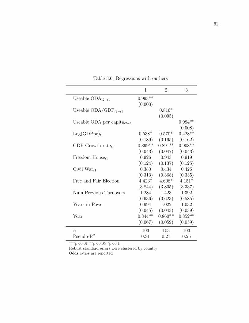
62

Table 3.6. Regressions with outliers

1 2 3

Useable ODAt2�t1 0.993**(0.003)

Useable ODA/GDPt2�t1 0.816*(0.095)

Useable ODA per capitat2�t1 0.984**(0.008)

Log(GDPpc)t1 0.538* 0.570* 0.428**(0.189) (0.195) (0.162)

GDP Growth ratet1 0.899** 0.891** 0.908**(0.043) (0.047) (0.043)

Freedom Houset1 0.926 0.943 0.919(0.124) (0.137) (0.125)

Civil Wart1 0.380 0.434 0.426(0.313) (0.368) (0.335)

Free and Fair Election 4.423* 4.608* 4.151*(3.844) (3.805) (3.337)

Num Previous Turnovers 1.284 1.423 1.392(0.636) (0.623) (0.585)

Years in Power 0.994 1.022 1.032(0.045) (0.043) (0.039)

Year 0.844** 0.860** 0.852**(0.067) (0.059) (0.059)

n 103 103 103Pseudo-R2 0.31 0.27 0.25

***p<0.01 **p<0.05 *p<0.1Robust standard errors were clustered by countryOdds ratios are reported

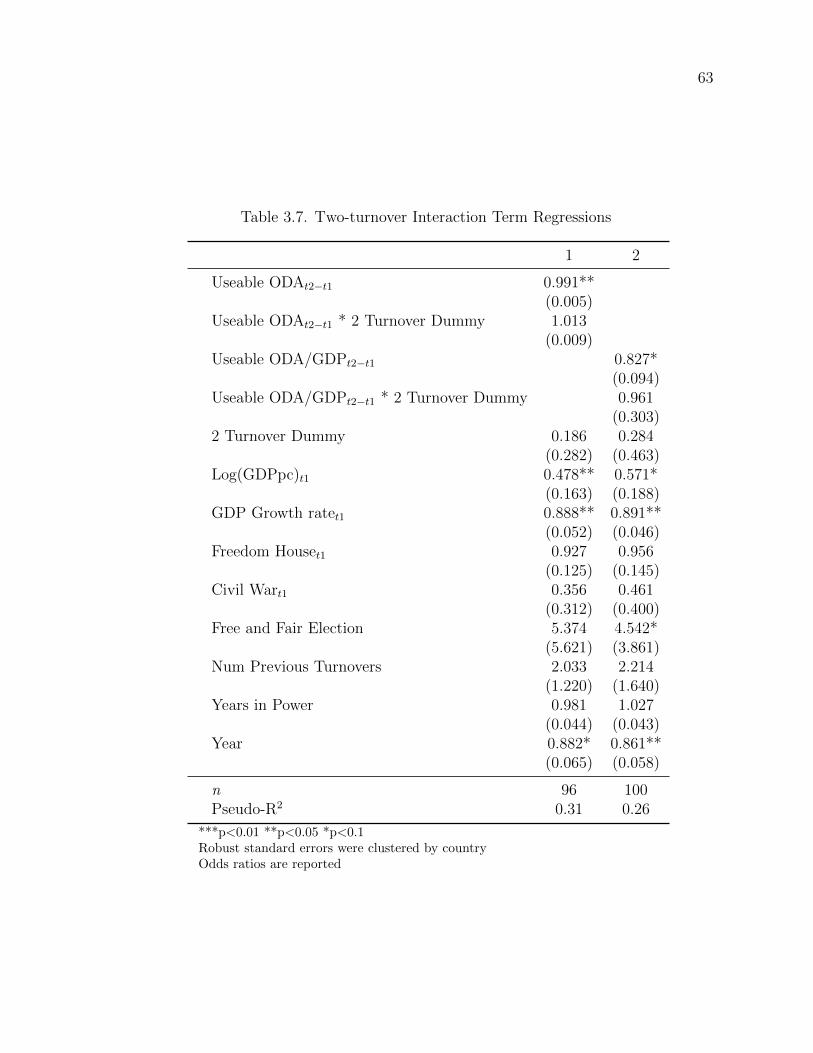
63

Table 3.7. Two-turnover Interaction Term Regressions

1 2

Useable ODAt2�t1 0.991**(0.005)

Useable ODAt2�t1 * 2 Turnover Dummy 1.013(0.009)

Useable ODA/GDPt2�t1 0.827*(0.094)

Useable ODA/GDPt2�t1 * 2 Turnover Dummy 0.961(0.303)

2 Turnover Dummy 0.186 0.284(0.282) (0.463)

Log(GDPpc)t1 0.478** 0.571*(0.163) (0.188)

GDP Growth ratet1 0.888** 0.891**(0.052) (0.046)

Freedom Houset1 0.927 0.956(0.125) (0.145)

Civil Wart1 0.356 0.461(0.312) (0.400)

Free and Fair Election 5.374 4.542*(5.621) (3.861)

Num Previous Turnovers 2.033 2.214(1.220) (1.640)

Years in Power 0.981 1.027(0.044) (0.043)

Year 0.882* 0.861**(0.065) (0.058)

n 96 100Pseudo-R2 0.31 0.26

***p<0.01 **p<0.05 *p<0.1Robust standard errors were clustered by countryOdds ratios are reported

64

CHAPTER 4

GHANA

On October 27, 1999, Ghana’s Minister of Finance, Victor Selormey, addressed

parliament on the state of the economy.1 This was an important speech, as the

economy was sluggish and an election was looming. While his comments were on the

general state of the economy, it was “the absence of donor funding that was at the

heart of the minister’s speech” and during the speech he claimed that less than 30%

of the aid that was committed to Ghana for 1999 had been disbursed (Economist

Intelligence Unit, 2000, p. 17). No one donor was responsible for this decline in aid.

It seems to have been due to exceptionally bad luck. Within Ghana, the decline

in aid led to declines in the provision of aid-funded goods and services to voters.

This was especially relevant in the provision of infrastructure to rural voters, as the

incumbent National Democratic Congress (NDC) government had won the previous

two elections with rural support and on a platform of providing services to rural

Ghanaians. The NDC lost the election in 2000. While many factors contributed to

this loss, one important factor was the decline in aid in 1999.

The Ghanaian case is well-predicted by the regression model in chapter 3 and

the theory outlined in chapter 2. Before the 2000 election, Ghana experienced an

unexpected reduction in aid and this led to a decline in the provision of infrastruc-

1The majority of this chapter was originally published in Briggs (2012).

65

ture and services to regular Ghanaians. Using data on electrification, this chapter

traces out how the processes linking the decline in aid lead to a decline in infrastruc-

ture provision and the decline in infrastructure to a decline in NDC support. The

chapter thus o↵ers support for the argument that aid changes influence incumbent

advantage. The chapter also examines the NDC’s ability to politically target aid

allocations and shows that both technocratic and political considerations influenced

which constituencies received electrification projects.

This chapter examines project aid for electrification.2 Section 4.1 discusses the

historical role of infrastructure provision and foreign aid in securing electoral majori-

ties for the NDC. Section 4.2 builds a model to examine how the NDC might have

wanted to allocate aid. It introduces the distinction between swing constituencies

and leaning swing constituencies and suggests that in Ghana an optimal electoral

strategy for the NDC was to target leaning swing constituencies instead of core or

regular swing areas. Section 4.3 shows that the NDC was able to exert political in-

fluence over which parts of Ghana received aid projects for electricity. I also exploit

a quasi-experiment to show that the NDC benefitted electorally from the electricity

projects that were completed in 1999. The analysis suggests that the NDC would

have done better at the polls if more aid had been disbursed in 1999. The chapter

concludes by discussing the generalizability of the empirical findings to the rest of

Ghana.

The Ghanaian case shows first that aid declines lead quickly to declines in

the roll out of goods and services to voters. When Ghana’s aid dropped in 1999,

actual spending on the development budget contracted by more than 30%. The

change in aid moved from donors to voters quickly enough that it could be felt

2The electricity sector was chosen for two reasons. First, aid for electricity was reduceddue to the 1999 aid cut. Second, detailed subnational information was available for the electricitysector. For a further explanation, see section 4.3.

66

within a year. By tracing out one process linking foreign resource disbursements

and voting patterns in specific constituencies, the chapter demonstrates that African

voters do vote retrospectively. While ethnicity may be a factor, African voters (like

voters elsewhere) are also influenced by changes in their standard of living. By

analyzing the NDC’s ability to influence where aid projects were built, the chapter

also reinforces the idea that incumbent governments will be better able to harness

aid for electoral aims if they have more discretion over funds (see table 2.1). It also

lends support to the idea that sometimes incumbent governments will have unique

and very context-dependent targeting strategies, such as the NDC strategy to target

leaning swing constituencies. Before moving to these details, it is useful to start with

an overview of why the NDC was so popular in the 1990s.

4.1 Who Supported the NDC in the 1990s and Why?

In 1992, the former dictator Jerry John Rawlings held Ghana’s first multiparty

elections since the founding elections of the brief Third Republic in 1979. Though

the opposition alleged foul play in 1992 and boycotted the parliamentary elections,

outside observers generally judged the election to have been fair (Je↵ries and Thomas,

1993). Rawlings won the 1992 election with over half of the vote in all regions except

Ashanti. Thus, even if there was some small-scale electoral fraud, it would not have

tipped the scales in favour of Rawlings (Je↵ries and Thomas, 1993, p. 356). The

next election, in 1996, returned the NDC and Rawlings to power. This election was

not boycotted and was even fairer than that of 1992 (Je↵ries, 1998). When his term

expired in 2000, Rawlings stepped aside and John Atta Mills ran for the NDC. The

2000 election was Ghana’s first experience of electoral turnover, with John A. Kufuor

of the New Patriotic Party (NPP) winning in a runo↵.3

3Ghana’s system requires that the winner of the Presidential election receive 50% +1 of thevote.

67

Ghana’s voting patterns have remained fairly constant since the 1992 election

(Je↵ries and Thomas, 1993; Nugent, 1999; Fridy, 2007). The NPP, which is generally

regarded as the more conservative party, tends to do better in urban areas and

around Kumasi.4 The NDC does well in rural areas and in Volta region, which

votes so consistently for the NDC that it is known as their “World Bank” of votes.5

The NDC’s popularity in poor and marginal areas is likely due to a combination of

pro-poor national policies and the extension of infrastructure and social services to

previously neglected areas of Ghana.

Before the 1992 election, the most important economic policy was the struc-

tural adjustment program (SAP). The SAP was started in 1983 and was quite suc-

cessful, as GDP growth between 1983 and 1992 averaging 5% per year and inflation

fell from 122% in 1983 to 10% in 1992 (Bawumia, 1998). The SAP was broadly

pro-poor and pro-rural, as it boosted agricultural earnings while concentrating costs

on cities. One example of this is the ratio of rural to urban consumer prices, which

increased from 0.83 in 1983 to 1.02 in 1991 (Bawumia, 1998, p. 59). Rural Ghana-

ians also benefited from the SAP’s provisions for the construction of infrastructure,

including roads, water, and electrification (Bawumia, 1998; Herbst, 1993; Tabatabai,

1986). Paul Nugent (1999, 2001, 2007) has argued that the NDC timed the provision

of electrification projects and roads to occur before elections and that this strategy

worked pretty well in 1992 and 1996.6

4Lindberg and Morrison (2005, p. 583) summarize Ghana’s voting breakdown succinctly,“In the stable two-party system in Ghana, rural belongingness, low levels of education, farmer andworking-class jobs, and low income signify a stable alignment with the leftist-oriented NDC, whereasthe opposite plus being employed in the public sector is typical of voting for the contemporaryexpression of the liberal, more right wing tradition in Ghanaian politics, the NPP.”

5This reference crops up uncited repeatedly in writing on Ghana’s elections. Andbo (2001)claims that Rawlings said that Volta was the NDC’s “World Bank” of votes to a reporter after the1992 election.

6Also see Killick (2010, p. 409–418) for a discussion of the importance of state spending toincumbency advantage in Ghana in the 1990s.

68

In 1996, the NDC’s emphasis on infrastructure provision was strengthened.

This is most obvious in the NDC’s campaign advertising, which included billboards

with the slogan “Always for People, Always for Development” beside a picture of

a rural area with roads and electric poles (Roberts, 1996). This imagery likely

resonated because of the NDC’s “undeniable progress in bringing electricity, water,

and roads to many rural areas over the years” (Roberts, 1996, p. 7). A reporter for

The Chronicle (2000) summarized the situation thusly:

“You see the period preceding the 1996 elections was the best for the ruralfolks. For the first time in decades, they began to feel that they were also‘somebodies.’ They were getting KVIPs, electricity, water and roads (thoughmost are impassable now). The money was there too, thanks to the WorldBank and the IMF. The farmers were also getting relatively better price [sic]for cocoa. In short, the rural people were comparatively ‘better o↵’ than theirurban counterparts who were struggling seriously to make ends meet.”

One author looked back on the 1990s and referred to the NDC’s political use

of development projects as their “development project vote-buying game” (Aubynn,

2002, p. 97). Some of this game was very likely played with foreign resources. In

1997, one year after the election, aid inflows to Ghana were equal to about half of

total investment (Leite et al., 1999, p. 16).

The NDC tried to play the same game before the 2000 election, but found

that they were heavily constrained by two shifts. First, in 1999 the government

experienced a terms-of-trade shock, as the prices for cocoa and gold both fell while the

price of oil rose.7 In 1999, the government’s cocoa duties were 150 billion cedi lower

than the previous year, and 100 billion cedi lower than were expected (Government

of Ghana, 2000). At the same time, the government also received 40 billion cedi (11

million USD) less than expected in grants and 235 billion cedi (67 million USD) less

7While the economy was clearly slowing down in 1999, the government actually collectedmore VAT than it originally predicted in that year.

69

than expected in project aid.8 This meant that in 1999, about a quarter of committed

project aid and 10% of grants were never disbursed. At the time Ghana was highly

aid-dependent, with foreign aid in 2001 equaling 64% of government expenditure

(World Bank, 2011).9

While finding reliable information on national government budgeting in the

early-to-mid 1990s is not straightforward, IMF reports suggest that throughout the

1990s foreign grants amounted to about 10% of the Ghanaian government’s annual

expenditure. Before 1994, the Ghanaian government received more in grants alone

than it spent on domestic capital formation. After 1994, the government increased

its spending on capital formation and from 1995–1998 foreign grants amounted to

about half of what the government spend on capital formation. Even when grants

are excluded, throughout the 1990s international donors funded more capital forma-

tion than the government (International Monetary Fund, 2000, p. 26). In 1997, aid

inflows to Ghana were equal to about half of total investment (Leite et al., 1999,

p. 16), and non-technical assistance, non-debt relief ODA averaged about 4.5% of

Ghana’s total GDP in the 1990s. Thus, aid provided a very large share of develop-

mental state spending. If development spending was helping the NDC stay in power,

then aid was helping the NDC stay in power.

In late October, 1999, the Ghanaian government announced that less than 30%

of the aid that was committed to Ghana for 1999 had been disbursed (Economist In-

telligence Unit, 2000, p. 17). These reductions in revenue and support led to declines

in the provision of services and infrastructure. The Finance Minister’s October 27th

speech, mentioned in the introduction, announced a 17% downwards revision of the

8The cedi exchange rate in 1999 was about 3,500 cedi per one US dollar, so a decline inproject assistance of 235 billion cedi represented a shortfall of about 67 million dollars.

9Information for 1998-2000 was unavailable so information for 2001 was used. The WorldBank 2000a has a slightly higher average figure of 68% over the period 1990-97.

70

government’s discretionary spending, which includes nearly all development projects.

An IMF report from November 1999 mentions that “the delays and shortfalls in ex-

ternal assistance in 1999 and deterioration in terms of trade by over 13 percent in

2000 substantially changed the medium-term outlook” (Leite et al., 1999, p. 49).

The World Bank (2000c, p. 2) also noted that “external budgetary support [in 1999]

was well below expected levels.” Notably, neither the IMF nor the World Bank—nor

any other consulted source—ascribed any intentionality to the aid reduction, and in

many ways Ghana was a star aid recipient. Instead the aid reduction seems like a

clear case of volatility in the aid system resulting in a large drop in aid to Ghana.

In 1999, Ghana simply had bad luck. Looking back on the previous year, the 2000

budget statement reveals that the decline in discretionary spending was real, and

much larger than the earlier estimate of 17%:

“When expenditures had to be restrained as a result of unfavourable fiscal con-ditions, it was those items that were considered purely discretionary that werea↵ected, namely, service and investment expenditures. In spite of this, not lessthan 60 percent of total estimates for those expenditure items were released toMDAs” (Government of Ghana, 2000, p. 16).

The NDC did not shy away from trumpeting the public works that it did

commission before the 2000 election, but there simply was not as much to boast

about (Gyimah-Boadi, 2001, p. 106).

In order to evaluate what might have happened if more aid was disbursed, it

is necessary to examine both the discretion that the NDC had in allocating donor

funds and the e↵ect that donor-funded projects had on vote patterns in the 2000

election. If we are confident that the NDC had a large amount of discretion over aid

allocation and that aid allocations led to more NDC votes, then we should be fairly

confident that the NDC would have done better had donors more fully disbursed the

foreign aid they had committed in 1999. In order to answer the first question, about

the degree of control that the NDC exercised over foreign aid resources, it is first

71

necessary to estimate where the NDC would have tried to allocate funds if it had a

completely free hand.

4.2 The NDC’s Allocative Strategies

This section builds a simple model to examine how a strategic incumbent party

would allocate aid if it had a free hand in doing so. It is reasonable to assume that

the incumbent party wants to win presidential elections for the foreseeable future,

and I would thus expect the incumbent party to allocate resources in an attempt

to gain votes. This suggests that the NDC in Ghana would allocate fewer than

expected resources to areas in Ashanti and Volta because both regions were already

largely committed—and viewed as committed—to political parties. In the words of

one NPP executive committee member who was interviewed while his party was in

power in 2005, “some [constituencies] we just ignore completely because whatever we

do we’ll lose” (Fridy, 2007, p. 2). Obviously these areas must receive some resources,

because over many elections they may come to resent being ‘taken for granted’ and so

may cease to be safe havens. Nevertheless, over reasonable time spans, an electorally

self-interested party would allocate fewer resources to these areas than other criteria,

such as measures of need, would suggest. The question then becomes, how should an

incumbent allocate resources among the parts of a country that are not committed?

At this point the incumbent party can choose to direct resources to areas that

lean towards or away from itself, or to areas that were evenly split.10 There are two

reasons why the government should target uncommitted voters that lean towards

the incumbent. The first reason assumes that the government has a multi-election

time horizon. If this is the case then one would expect that parts of the country

10Ghana has an absolute majority system for electing the president. If no candidate reaches50% + 1 then there is a runo↵ between the top two candidates. This model would have to bemodified if applied to other contexts.

72

would tend to shift their allegiances in response to the flow of resources in earlier

time periods. Funding uncommitted areas that lean towards your party would thus

give an incentive to all swing voters to move towards the incumbent party in the next

election. By the same token, if the incumbent directed more resources to areas that

leaned away from his party, then he would be encouraging future voters to vote for the

opposition. This e↵ect on the next election matters because there is no unambiguous

theory to guide the incumbent if we only consider the e↵ect of resources on votes in

the present election. Areas that lean towards the opposition provide more possible

votes to switch, but given a secret ballot and low monitoring potential, resources

can only induce voters to switch if voters acknowledge the support of the incumbent,

which is more likely in areas where the incumbent is more popular (Nugent, 2007).

Of course, the areas that already lean towards the incumbent—and thus are most

likely to acknowledge the incumbent’s resources—o↵er fewer switchable votes. In

this simple model this result in indi↵erence between the two choices in the current

election, and this is why e↵ect on the future elections is so important to targeting.11

A second reason why the incumbent should target friendly voters is because they

represent a less risky political investment than targeting voters that lean towards

opposition parties (Cox and McCubbins, 1986). This will only hold if incumbents

are risk averse.

This is an extremely simplified version of Ghana’s politics, but it does provide

a general guide as to how one might expect the incumbent NDC to target resources.

First, we would expect the NDC to want to spend less on committed areas like

Ashanti or Volta. Second, we would expect the NDC to want to direct more resources

11This argument can be extended and tested in various ways. For example, this argumentrequires multi-election time horizons and so should be applicable only in countries with either noterm limits or fairly entrenched party systems. We would not expect consistent targeting of leaningbut uncommitted voters in a country with term limits and a highly personalized political systembecause incumbents do not have time horizons that span many elections. In these political systemsterm limits may provide a point where one can test the influence of time horizons.

73

to the parts of the country that are non-committed but lean towards the NDC.

Third, we would expect that while Volta and Ashanti both will receive lower levels

of resources than other criteria (such as population) would suggest, Volta should

generally be treated better than Ashanti, because it is the safe haven of the incumbent

NDC and Ashanti is the safe haven of the out-of-power NPP party. In general then,

more votes for the incumbent should translate into more resources in future elections,

but this pattern will not hold in areas that are considered committed to either major

party.

4.3 The Causes and E↵ects of Aid in Ghana

During the 1990s and early 2000s, the Ghanaian Ministry of Finance did not

keep centralized subnational information on aid disbursements. At the Ministry level,

record keeping on aid was generally uneven and sparse. In order to examine how

the NDC actually allocated foreign assistance, I circumvented these data issues by

collecting subnational allocation information on the National Electrification Project

(NEP), a large World Bank and bilateral donor-funded infrastructure program that

ran from 1993–1999.12 Infrastructure for electricity was in short supply throughout

the 1990s. The World Bank estimated that in 1990, 70% of Ghanaians consumed

energy generated from burning wood or agricultural waste, 20% gained access to

energy through petroleum products, and 10% had access to grid-powered electricity

(1993, p. 1–4). The Ghanaian government conducted a survey in 1991/92 that

estimated that while 24% of all Ghanaians had access to some form of electricity,

rural access to electricity was estimated at 5% (Ghana Statistical Service, 1992).

Figure 4.5 shows that aside from Greater Accra and Ashanti, access to electricity

was very low. It was almost 0% in the two northernmost regions of Upper West

12While it would have been preferable to gather data on all aid for infrastructure allocationsacross Ghana, these data were unavailable.

74

and Upper East. It is thus not surprising that the electrification program was very

popular with rural Ghanaians.

4.3.1 The National Electrification Project

While the NEP is only a single program, it grew out of a Ghanaian and World

Bank e↵ort to ameliorate the situation described above. The primary goal of the

NEP was to erect high voltage power lines across Ghana, especially in the rural

areas that completely lacked grid power. This build-out would connect 27 district

capitals to the grid and would create the high voltage network that then would allow

smaller, low-voltage lines to branch o↵ towards towns. It consisted of 29 sub-projects

spread across all 10 regions. In addition to the high-voltage lines and the district

capitals, the project was also initially expected to electrify about 530 towns.13

Thus, while this Chapter only analyzes one aid project, it is one that covered an

entire sector and laid the foundations for future electrification in Ghana. While there

were other electrification projects active at the time, such as Self-Help Electrification

Projects (SHEPs), all of them hinged on having a high voltage power line nearby.

The NEP was building those lines across the country, and thus it structured who

could get electricity in the future. The plan for this project was finalized in 1993,

one year after Ghana’s turn back to multi-partyism. The next sections examines how

NEP resources were allocated within Ghana and compares the allocations against

vote returns for the NDC in 1992, the year before the plan for the NEP was finalized.

4.3.2 Targeting at the Regional Level

By and large, the regional dispersion of NEP resources did approximate the

model laid out above. At the start of the NEP, every area of Ghana had a large

13In the World Bank Sta↵ Appraisal Report (World Bank, 1993) this was revised downwardto 434 towns.

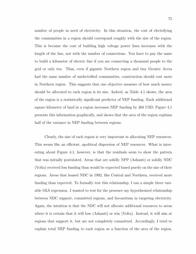
75

number of people in need of electricity. In this situation, the cost of electrifying

the communities in a region should correspond roughly with the size of the region.

This is because the cost of building high voltage power lines increases with the

length of the line, not with the number of connections. You have to pay the same

to build a kilometer of electric line if you are connecting a thousand people to the

grid or only ten. Thus, even if gigantic Northern region and tiny Greater Accra

had the same number of unelectrified communities, construction should cost more

in Northern region. This suggests that one objective measure of how much money

should be allocated to each region is its size. Indeed, as Table 4.1 shows, the area

of the region is a statistically significant predictor of NEP funding. Each additional

square kilometer of land in a region increases NEP funding by 268 USD. Figure 4.1

presents this information graphically, and shows that the area of the region explains

half of the variance in NEP funding between regions.

Clearly, the size of each region is very important in allocating NEP resources.

This seems like an e�cient, apolitical dispersion of NEP resources. What is inter-

esting about Figure 4.1, however, is that the residuals seem to show the pattern

that was initially postulated. Areas that are solidly NPP (Ashanti) or solidly NDC

(Volta) received less funding than would be expected based purely on the size of their

regions. Areas that leaned NDC in 1992, like Central and Northern, received more

funding than expected. To formally test this relationship, I ran a simple three vari-

able OLS regression. I wanted to test for the presence my hypothesized relationship

between NDC support, committed regions, and favouritism in targeting electricity.

Again, the intuition is that the NDC will not allocate additional resources to areas

where it is certain that it will lose (Ashanti) or win (Volta). Instead, it will aim at

regions that support it, but are not completely committed. Accordingly, I tried to

explain total NEP funding to each region as a function of the area of the region,

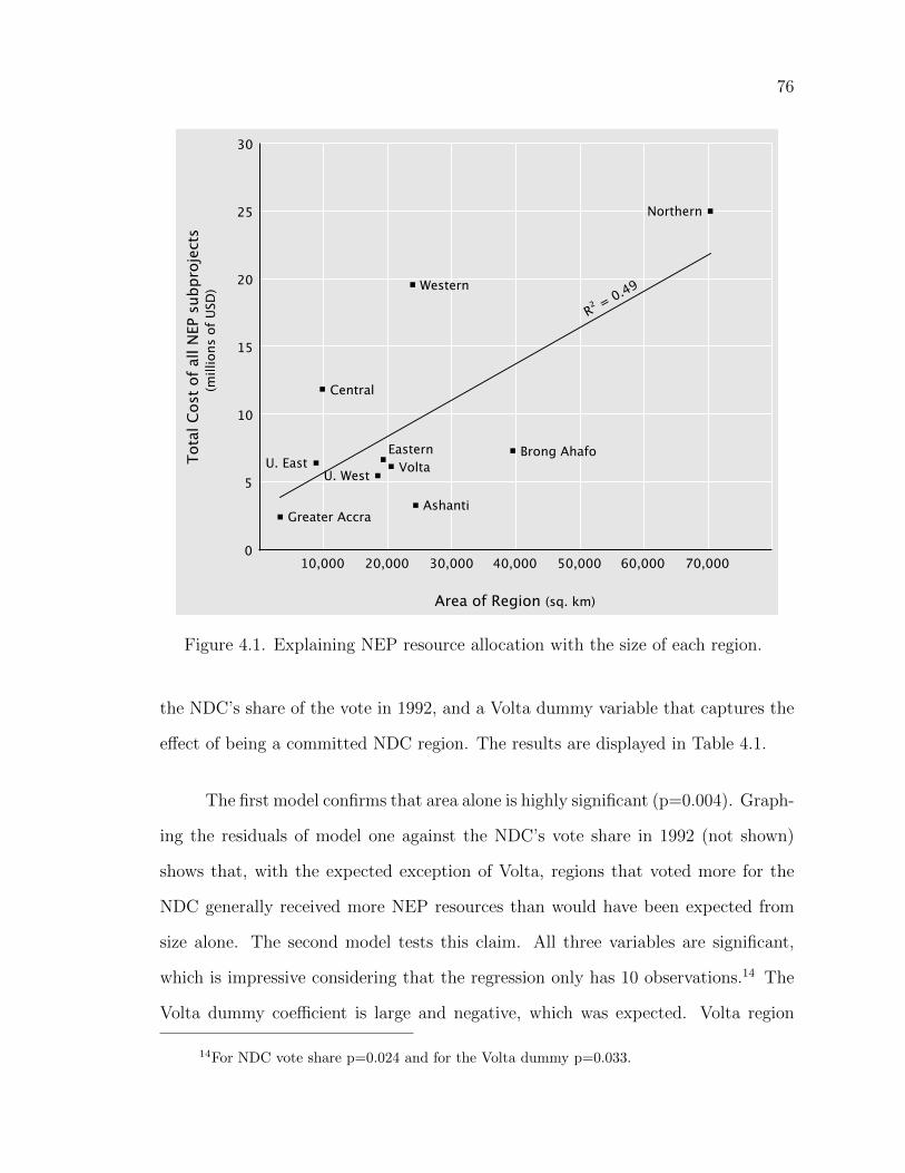
76

10,000 20,000 30,000 40,000 50,000 60,000 70,000

30

0

5

10

15

20

25

Area of Region (sq. km)

Tot

al C

ost

of a

ll N

EP s

ubpro

ject

s

(mill

ions

of

USD

) Western

Northern

Central

Greater Accra

Volta

Ashanti

Brong Ahafo

U. West

U. East

EasternVoltaU. East

R² = 0.49

Figure 4.1. Explaining NEP resource allocation with the size of each region.

the NDC’s share of the vote in 1992, and a Volta dummy variable that captures the

e↵ect of being a committed NDC region. The results are displayed in Table 4.1.

The first model confirms that area alone is highly significant (p=0.004). Graph-

ing the residuals of model one against the NDC’s vote share in 1992 (not shown)

shows that, with the expected exception of Volta, regions that voted more for the

NDC generally received more NEP resources than would have been expected from

size alone. The second model tests this claim. All three variables are significant,

which is impressive considering that the regression only has 10 observations.14 The

Volta dummy coe�cient is large and negative, which was expected. Volta region

14For NDC vote share p=0.024 and for the Volta dummy p=0.033.

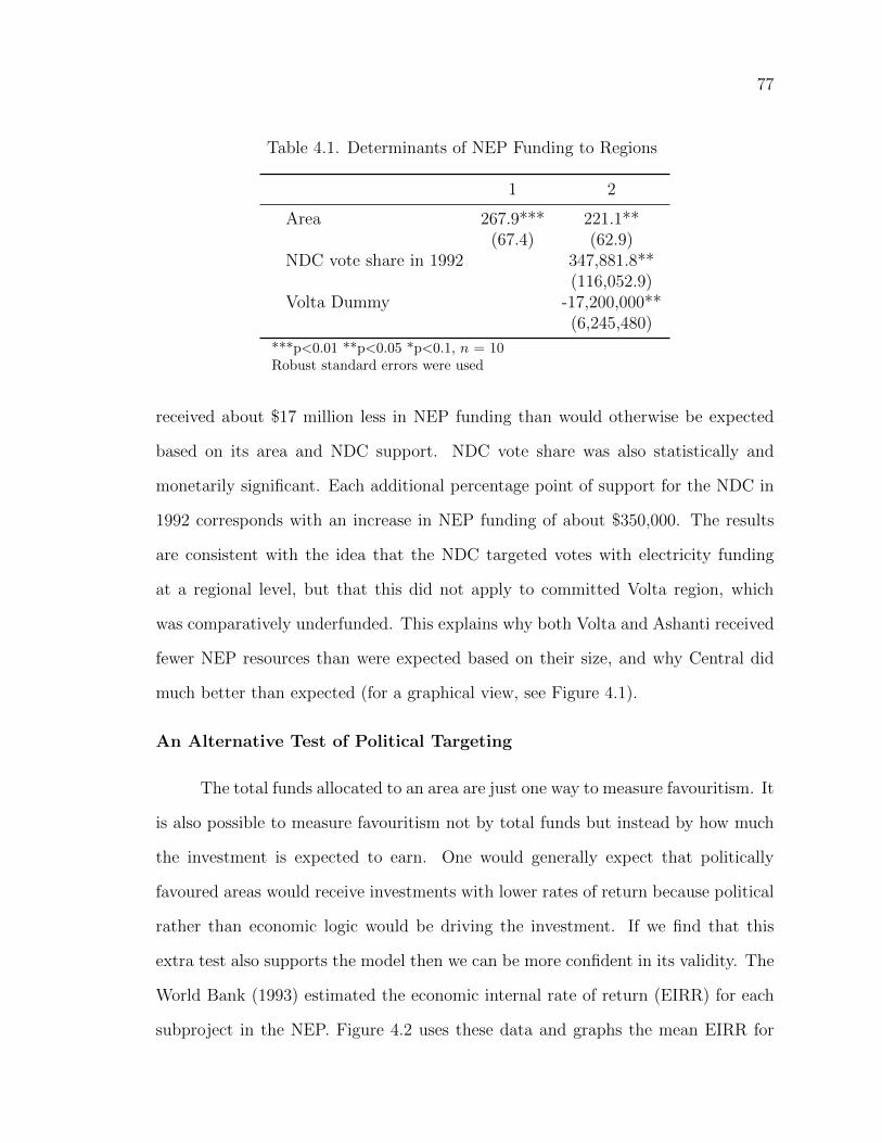
77

Table 4.1. Determinants of NEP Funding to Regions

1 2

Area 267.9*** 221.1**(67.4) (62.9)

NDC vote share in 1992 347,881.8**(116,052.9)

Volta Dummy -17,200,000**(6,245,480)

***p<0.01 **p<0.05 *p<0.1, n = 10Robust standard errors were used

received about $17 million less in NEP funding than would otherwise be expected

based on its area and NDC support. NDC vote share was also statistically and

monetarily significant. Each additional percentage point of support for the NDC in

1992 corresponds with an increase in NEP funding of about $350,000. The results

are consistent with the idea that the NDC targeted votes with electricity funding

at a regional level, but that this did not apply to committed Volta region, which

was comparatively underfunded. This explains why both Volta and Ashanti received

fewer NEP resources than were expected based on their size, and why Central did

much better than expected (for a graphical view, see Figure 4.1).

An Alternative Test of Political Targeting

The total funds allocated to an area are just one way to measure favouritism. It

is also possible to measure favouritism not by total funds but instead by how much

the investment is expected to earn. One would generally expect that politically

favoured areas would receive investments with lower rates of return because political

rather than economic logic would be driving the investment. If we find that this

extra test also supports the model then we can be more confident in its validity. The

World Bank (1993) estimated the economic internal rate of return (EIRR) for each

subproject in the NEP. Figure 4.2 uses these data and graphs the mean EIRR for

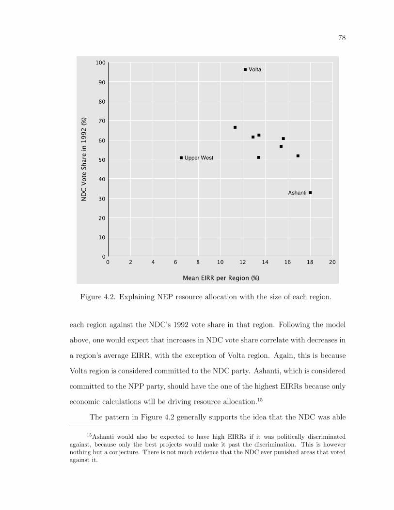
78

200 2 4 6 8 10 12 14 16 18

100

0

10

20

30

40

50

60

70

80

90

Mean EIRR per Region (%)

ND

C V

ote

Shar

e in

19

92

(%

)

Volta

Upper West

Ashanti

Figure 4.2. Explaining NEP resource allocation with the size of each region.

each region against the NDC’s 1992 vote share in that region. Following the model

above, one would expect that increases in NDC vote share correlate with decreases in

a region’s average EIRR, with the exception of Volta region. Again, this is because

Volta region is considered committed to the NDC party. Ashanti, which is considered

committed to the NPP party, should have the one of the highest EIRRs because only

economic calculations will be driving resource allocation.15

The pattern in Figure 4.2 generally supports the idea that the NDC was able

15Ashanti would also be expected to have high EIRRs if it was politically discriminatedagainst, because only the best projects would make it past the discrimination. This is howevernothing but a conjecture. There is not much evidence that the NDC ever punished areas that votedagainst it.

79

to use politics to influence NEP allocations. Volta has higher EIRRs than its vote

share would suggest, Ashanti predictably has the highest EIRRs and the lowest level

of NDC support, and the regions in the middle generally fit the pattern of increasing

NDC vote shares correlation with declining EIRRs. Interestingly, while Ashanti has

the highest EIRRs it also has the lowest mean level of funding per subproject. This

means that the region with the highest rates of return on its subprojects received the

lowest level of funding per subproject. The only unexpected result was the outlier

of Upper West region. The average rate of return on the subprojects in Upper West

was so low that it was expected to lose money over time (it had a negative net

present value). While Upper West is generally considered an (uncommitted) NDC

area (Fridy, 2007), EIRRs this low are strange. The World Bank sta↵ appraisal of

the NEP justified this investment by first pointing out that it would not be funding

this segment of the NEP,16 and then stating that:

“inclusion of these sub-projects is also deemed justified considering that theproject is designed to contribute to balanced regional development and equityin the country and that supply from the national grid is the least-cost solution,as well as taking into account that the cost involved is relatively small” (WorldBank, 1993, Annex 3-14).

The issues that the World Bank raised in defense of the investment—balanced

regional development and equity—need to be taken seriously and pose a major prob-

lem for regional-level analyses. While the results above are suggestive, the problem

with all of them is that at a regional level poverty and NDC support overlap almost

perfectly. Thus, the relationship between total funding allocation and EIRR spreads

could be being driven by measures of poverty or a desire to improve the status of

marginal regions in Ghana. This makes it very di�cult to convincingly show political

16The Upper West sub-projects were funded by DANIDA (World Bank, 1993, Annex 3-5).The fact that the World Bank pointed this out makes one wonder if they had not considered thatthese resources are all interchangeable, and that if DANIDA hadn’t funded section then the Bankwould have had fewer resources for elsewhere.

80

targeting at a regional level. It is possible that poorer areas were more likely to vote

NDC and that the NDC was targeting poverty with electrification.17 To remedy this

deficiency, I also collected data on NEP spending at the smallest political unit in

Ghana, the constituency. This enabled me to test for the influence of politics on aid

allocation across very similar units.

4.3.3 Targeting at the Constituency Level

Analyzing subnational units is a common way to increase the number of obser-

vations in an analysis (King et al., 1994), and in this case it also helps to control for

confounding variables such as the fraction of the population that is urban and has ac-

cess to better infrastructure. I received a list of all communities that were electrified

in Upper West and Upper East provinces, along with the date of electrification, from

the Ministry of Energy.18 This list was checked against the original NEP Feasibility

Study by Acres International, the World Bank implementation completion report,

and annual reports from the Volta River Authority. Additionally, an interview with

a former Northern Electricity Department (NED) manager confirmed the accuracy

of my list. While it would have been preferable to receive a list of all electrified

communities in all of Ghana, NEP record keeping was uneven. The Northern Elec-

tricity Department, a subsidiary of the Volta River Authority, was responsible for

electrification in the Northern part of the country and kept much better records than

17The NDC was not spending more NEP resources in areas with the largest populationwithout electricity. While the size of a region is a robust predictor of NEP funding, the estimatednumber of people per region without electricity in 1991 is insignificant. This makes sense, becauseeach region had a fairly large share of the population without electricity and most of the costs ofelectrification increase in area rather than in population.

18While it would have been preferable to receive a broader list of all donor-funded electrifica-tion programs in 1999 this information was unavailable. Electrification was broken down by projectand not funder, but thanks to the excellent record keeping of the Northern Electricity Department(NED), an organization under the Volta River Authority, I was able to obtain a list of villages andthe year they were electrified under the donor-funded NEP. This list excluded Northern region, andI am still in contact with people at the NED who are trying to locate this information.

81

the Electricity Corporation of Ghana, which was responsible for the South. I thus

restrict my constituency-level analysis to Ghana’s northern-most provinces. Later in

the paper I discuss how this a↵ects the generalizability of my results.

In the two northern regions of Ghana there are 11 districts, which in total con-

tain 20 constituencies. Of these, twelve constituencies fall inside ‘ordinary’ districts

and eight fall within ‘municipal’ districts. Ordinary districts are more rural, and

thus are less likely to already have services or infrastructure such as electricity. The

fourth Ghana Living Standards Survey (Ghana Statistical Service, 1999) found the

level of access to grid-powered electricity to be 0% in Upper West and 4% in Upper

East.19 It is safe to assume that the 4% electricity access in Upper East would have

all been concentrated in municipal districts of Bawku East or Bolgatanga, which

first received limited electricity in 1992 and 1989, respectively. This means that as of

1998, before the NEP reached the far north, the rural constituencies in Upper East

and Upper West had no grid-powered electricity.

The analysis is limited to constituencies in rural (or ‘ordinary’) districts not

only to remove the influence of prior electrification but also to limit the influence

of urbanization, which is my main confounding variable and covaries with many

other possibly relevant omitted variables.20 Table 4.2 shows how urbanization, the

rate of literacy, and access to piped water vary within ordinary (rural) districts.

Census data is recorded at the district rather than constituency level, so the ordinary

19The 95% confidence interval for Upper East was between 1.8% and 6.7%. There is noconfidence interval for Upper West because no one surveyed (out of 120 people) had grid-poweredelectricity. The survey was carried out in 1998, before NEP construction began. It is likely that therewas electricity in the Upper West before the NEP, because the Volta River Authority completeda grid extension project that involved the Upper West on September 21, 1996. However, thisextension only involved construction in the municipal district of Wa.

20Urbanization and electricity provision are both so low in ordinary districts, that they arealmost 0 in the 1991/92 and 1998/99 Ghana Living Standards Surveys 1992; 1999. Some municipaldistricts have electrification, and the mean rate of urbanization across municipal districts is 20%higher than in ordinary districts.

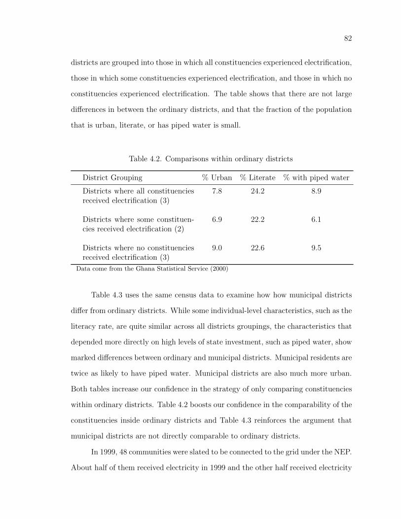
82

districts are grouped into those in which all constituencies experienced electrification,

those in which some constituencies experienced electrification, and those in which no

constituencies experienced electrification. The table shows that there are not large

di↵erences in between the ordinary districts, and that the fraction of the population

that is urban, literate, or has piped water is small.

Table 4.2. Comparisons within ordinary districts

District Grouping % Urban % Literate % with piped water

Districts where all constituenciesreceived electrification (3)

7.8 24.2 8.9

Districts where some constituen-cies received electrification (2)

6.9 22.2 6.1

Districts where no constituenciesreceived electrification (3)

9.0 22.6 9.5

Data come from the Ghana Statistical Service (2000)

Table 4.3 uses the same census data to examine how how municipal districts

di↵er from ordinary districts. While some individual-level characteristics, such as the

literacy rate, are quite similar across all districts groupings, the characteristics that

depended more directly on high levels of state investment, such as piped water, show

marked di↵erences between ordinary and municipal districts. Municipal residents are

twice as likely to have piped water. Municipal districts are also much more urban.

Both tables increase our confidence in the strategy of only comparing constituencies

within ordinary districts. Table 4.2 boosts our confidence in the comparability of the

constituencies inside ordinary districts and Table 4.3 reinforces the argument that

municipal districts are not directly comparable to ordinary districts.

In 1999, 48 communities were slated to be connected to the grid under the NEP.

About half of them received electricity in 1999 and the other half received electricity

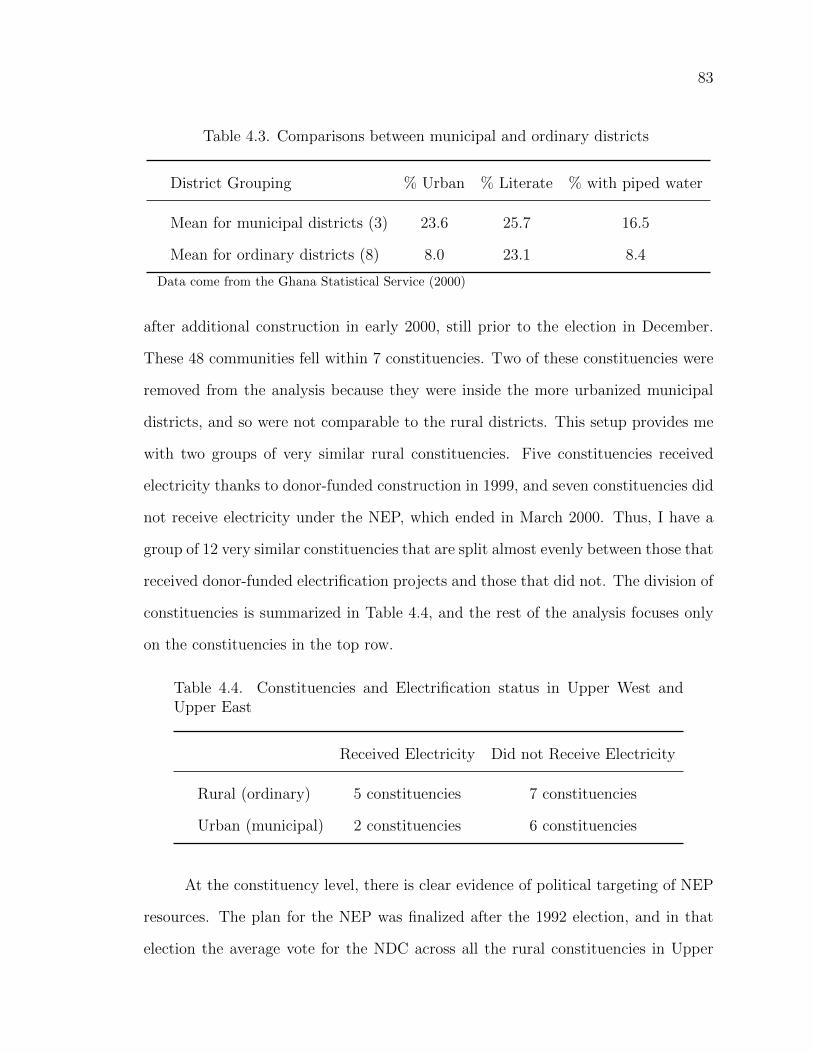
83

Table 4.3. Comparisons between municipal and ordinary districts

District Grouping % Urban % Literate % with piped water

Mean for municipal districts (3) 23.6 25.7 16.5

Mean for ordinary districts (8) 8.0 23.1 8.4

Data come from the Ghana Statistical Service (2000)

after additional construction in early 2000, still prior to the election in December.

These 48 communities fell within 7 constituencies. Two of these constituencies were

removed from the analysis because they were inside the more urbanized municipal

districts, and so were not comparable to the rural districts. This setup provides me

with two groups of very similar rural constituencies. Five constituencies received

electricity thanks to donor-funded construction in 1999, and seven constituencies did

not receive electricity under the NEP, which ended in March 2000. Thus, I have a

group of 12 very similar constituencies that are split almost evenly between those that

received donor-funded electrification projects and those that did not. The division of

constituencies is summarized in Table 4.4, and the rest of the analysis focuses only

on the constituencies in the top row.

Table 4.4. Constituencies and Electrification status in Upper West andUpper East

Received Electricity Did not Receive Electricity

Rural (ordinary) 5 constituencies 7 constituencies

Urban (municipal) 2 constituencies 6 constituencies

At the constituency level, there is clear evidence of political targeting of NEP

resources. The plan for the NEP was finalized after the 1992 election, and in that

election the average vote for the NDC across all the rural constituencies in Upper

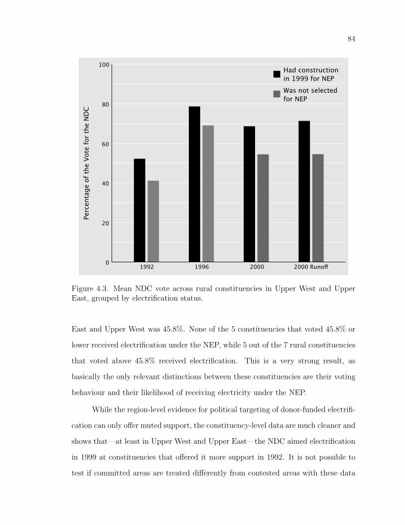
84

100

0

20

40

60

80

Perc

enta

ge o

f th

e Vo

te f

or t

he N

DC

1992 1996 2000 2000 Runoff

Had constructionin 1999 for NEP

Was not selectedfor NEP

Figure 4.3. Mean NDC vote across rural constituencies in Upper West and UpperEast, grouped by electrification status.

East and Upper West was 45.8%. None of the 5 constituencies that voted 45.8% or

lower received electrification under the NEP, while 5 out of the 7 rural constituencies

that voted above 45.8% received electrification. This is a very strong result, as

basically the only relevant distinctions between these constituencies are their voting

behaviour and their likelihood of receiving electricity under the NEP.

While the region-level evidence for political targeting of donor-funded electrifi-

cation can only o↵er muted support, the constituency-level data are much cleaner and

shows that—at least in Upper West and Upper East—the NDC aimed electrification

in 1999 at constituencies that o↵ered it more support in 1992. It is not possible to

test if committed areas are treated di↵erently from contested areas with these data

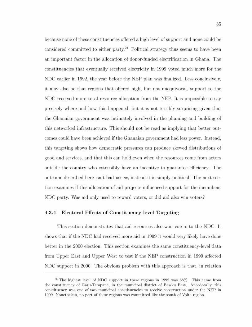
85

because none of these constituencies o↵ered a high level of support and none could be

considered committed to either party.21 Political strategy thus seems to have been

an important factor in the allocation of donor-funded electrification in Ghana. The

constituencies that eventually received electricity in 1999 voted much more for the

NDC earlier in 1992, the year before the NEP plan was finalized. Less conclusively,

it may also be that regions that o↵ered high, but not unequivocal, support to the

NDC received more total resource allocation from the NEP. It is impossible to say

precisely where and how this happened, but it is not terribly surprising given that

the Ghanaian government was intimately involved in the planning and building of

this networked infrastructure. This should not be read as implying that better out-

comes could have been achieved if the Ghanaian government had less power. Instead,

this targeting shows how democratic pressures can produce skewed distributions of

good and services, and that this can hold even when the resources come from actors

outside the country who ostensibly have an incentive to guarantee e�ciency. The

outcome described here isn’t bad per se, instead it is simply political. The next sec-

tion examines if this allocation of aid projects influenced support for the incumbent

NDC party. Was aid only used to reward voters, or did aid also win voters?

4.3.4 Electoral E↵ects of Constituency-level Targeting

This section demonstrates that aid resources also won voters to the NDC. It

shows that if the NDC had received more aid in 1999 it would very likely have done

better in the 2000 election. This section examines the same constituency-level data

from Upper East and Upper West to test if the NEP construction in 1999 a↵ected

NDC support in 2000. The obvious problem with this approach is that, in relation

21The highest level of NDC support in these regions in 1992 was 68%. This came fromthe constituency of Garu-Tempane, in the municipal district of Bawku East. Anecdotally, thisconstituency was one of two municipal constituencies to receive construction under the NEP in1999. Nonetheless, no part of these regions was committed like the south of Volta region.

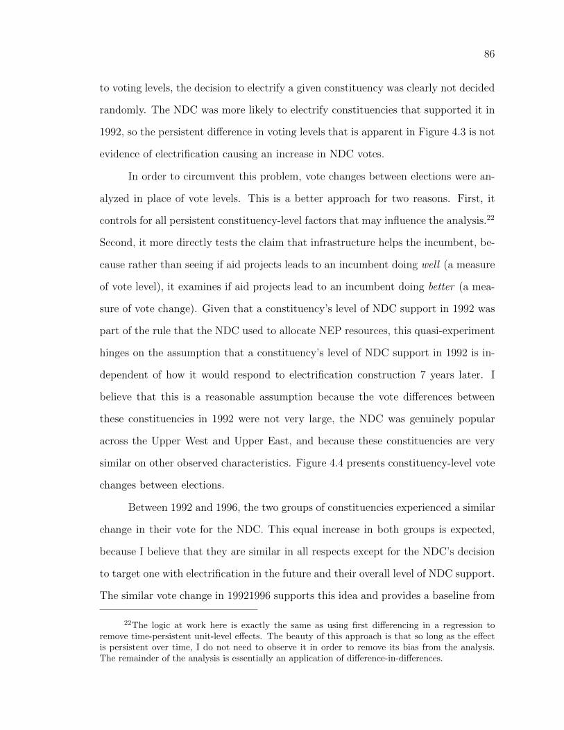
86

to voting levels, the decision to electrify a given constituency was clearly not decided

randomly. The NDC was more likely to electrify constituencies that supported it in

1992, so the persistent di↵erence in voting levels that is apparent in Figure 4.3 is not

evidence of electrification causing an increase in NDC votes.

In order to circumvent this problem, vote changes between elections were an-

alyzed in place of vote levels. This is a better approach for two reasons. First, it

controls for all persistent constituency-level factors that may influence the analysis.22

Second, it more directly tests the claim that infrastructure helps the incumbent, be-

cause rather than seeing if aid projects leads to an incumbent doing well (a measure

of vote level), it examines if aid projects lead to an incumbent doing better (a mea-

sure of vote change). Given that a constituency’s level of NDC support in 1992 was

part of the rule that the NDC used to allocate NEP resources, this quasi-experiment

hinges on the assumption that a constituency’s level of NDC support in 1992 is in-

dependent of how it would respond to electrification construction 7 years later. I

believe that this is a reasonable assumption because the vote di↵erences between

these constituencies in 1992 were not very large, the NDC was genuinely popular

across the Upper West and Upper East, and because these constituencies are very

similar on other observed characteristics. Figure 4.4 presents constituency-level vote

changes between elections.

Between 1992 and 1996, the two groups of constituencies experienced a similar

change in their vote for the NDC. This equal increase in both groups is expected,

because I believe that they are similar in all respects except for the NDC’s decision

to target one with electrification in the future and their overall level of NDC support.

The similar vote change in 19921996 supports this idea and provides a baseline from

22The logic at work here is exactly the same as using first di↵erencing in a regression toremove time-persistent unit-level e↵ects. The beauty of this approach is that so long as the e↵ectis persistent over time, I do not need to observe it in order to remove its bias from the analysis.The remainder of the analysis is essentially an application of di↵erence-in-di↵erences.

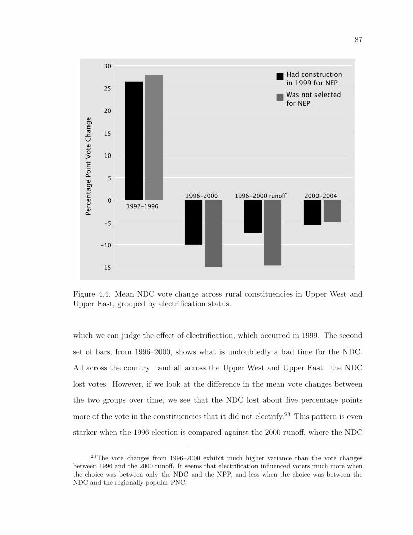
87

30

-15

-10

-5

0

5

10

15

20

25Pe

rcen

tage

Poi

nt V

ote

Cha

nge

Had constructionin 1999 for NEP

Was not selectedfor NEP

1992-1996

1996-2000 1996-2000 runoff 2000-2004

Figure 4.4. Mean NDC vote change across rural constituencies in Upper West andUpper East, grouped by electrification status.

which we can judge the e↵ect of electrification, which occurred in 1999. The second

set of bars, from 1996–2000, shows what is undoubtedly a bad time for the NDC.

All across the country—and all across the Upper West and Upper East—the NDC

lost votes. However, if we look at the di↵erence in the mean vote changes between

the two groups over time, we see that the NDC lost about five percentage points

more of the vote in the constituencies that it did not electrify.23 This pattern is even

starker when the 1996 election is compared against the 2000 runo↵, where the NDC

23The vote changes from 1996–2000 exhibit much higher variance than the vote changesbetween 1996 and the 2000 runo↵. It seems that electrification influenced voters much more whenthe choice was between only the NDC and the NPP, and less when the choice was between theNDC and the regionally-popular PNC.

88

lost about seven percentage points more in constituencies that it did not electrify.

We can gain confidence that the divergence in 1996–2000 is due to electrification by

looking at the di↵erence in vote changes between 2000–2004. In this period, as in

1992–1996, there were no new events that divided the two groups and, as expected,

the di↵erence in mean vote changes between the two groups of constituencies is only

half of one per cent.

In relation to vote changes, the only relevant distinction between the two

groups of constituencies is that one received construction as part of the NEP in

1999. Both groups saw their mean voting behaviour move in essentially the same

pattern between 1992–1996 and 2000–2004, but the voting behaviour of the groups

diverged in the period 1996–2000, when the only significant di↵erence between the

two groups was that one received aid-funded electrification. While the two groups

do di↵er in terms of their overall level of support for the NDC, they only experienced

di↵erent vote changes during the electrification period. This is strong evidence for

the claim that electrification projects increased NDC support.

4.3.5 Validity and the Counter Factual

What would have happened if the NDC had received more aid and was able

to build more infrastructure in 1999? The previous analysis suggests that the NDC

would have done better in the 2000 election. However, the quasi-experiment only

examined twelve very similar, rural constituencies in similar regions, and in doing so

it sacrificed external validity for internal validity. While we can be quite confident

in the logic and rigour of the quasi-experiment, the results cannot be immediately

generalized to the rest of Ghana. Specifically, my quasi-experiment looked at electri-

fication in rural constituencies in northern regions. Therefore, I cannot immediately

generalize to other types of infrastructure, to urban areas, or to other regions. Before

I can address the core question of if the NDC would have done appreciably better

89

if more aid had been disbursed, I need to examine these three points to see how

broadly I can apply my analysis.

Other Forms of Infrastructure

The examination of the e↵ects of infrastructure provision only analyzed the

electoral e↵ects of an electrification project, so it is worth considering if there is

something special about electricity provision, and if voters might respond di↵erently

to electrification than to road construction or the provision of piped water. While it

is quite possible that voters respond more (or less) to electrification than other forms

of infrastructure or services, it is unlikely that voters only respond to electricity. For

example, Harding (2011) found that Ghanaian voters were similarly responsive to

the provision of roads. Indeed, the NDC’s explicit strategy and election advertising,

as well as press reports and academic analyses, bundle water, roads, and electricity

provision into a ‘developmental package’ that the NDC promised to provide. Ideally,

the analysis would include many more forms of infrastructure in Ghana in 1999,

but the data simply were not available. This issue should make us skeptical of the

magnitude of the e↵ect of other forms of infrastructure provision, but the likely

direction of the e↵ect seems clear. Other forms of infrastructure also would have

helped the NDC, though perhaps not to the same degree.

The Rural/Urban Divide

The comparison was drawn across rural constituencies and there are no empir-

ical or theoretical grounds to expect it to hold in urban areas. This limits the scope

of the analysis to rural areas, but in 2000 urbanites only made up 44% of Ghana’s to-

tal population (Ghana Statistical Service, 2000). Based on the NDC’s track record,

its stated intentions, and the previous analysis of NEP targeting, it is very likely

that any increases in infrastructure or service provision in 1999 would have targeted

90

Ghana’s rural majority. The prior analysis of northern rural voters shows that they

would likely have responded by increasing their support for the NDC.

Regions and Language

Even if the analysis is restricted to rural areas and we believe that all forms

of infrastructure influence voters to roughly the same degree, it is still possible that

rural areas in di↵erent regions may respond di↵erently to infrastructure provision.

There may, for example, be something peculiar about rural constituencies in Up-

per West and Upper East that prevents them from being compared to rural areas

in Northern or Western regions. These regional di↵erences could exist because of

di↵erences in the base level of services or infrastructure across regions. As Table

4.5 shows, this is unlikely as the rate of electrification, especially rural electrifica-

tion, was low everywhere. While there may soon be a point in time when basic

infrastructure such as electricity or roads are so prevalent in rural Ghana that ad-

ditional extensions will su↵er from rapidly diminishing marginal returns, that time

has not yet come and it certainly did not exist in 1999. While Upper East and

Upper West do have especially low electrification rates (a factor which increased the

internal validity of the quasi-experiment), rural areas across Ghana are clearly not

near the point where the government would face declining marginal political returns

to infrastructure spending.

Of the other factors that may skew rural voting across regions, language is

the most convincing. Fridy (2007) has shown that language groups are especially

good predictors of party support, with Ewe speakers favouring the NDC and Akan

speakers favouring the NPP. Thus, it is reasonable to expect that Ewe and Akan-

speakers may respond di↵erently to government spending than other groups, such as

those in the north. Hypothetically, I will take the extreme position that Ewe speakers,

Akan speakers, and all urbanites would not be swayed at all by new infrastructure

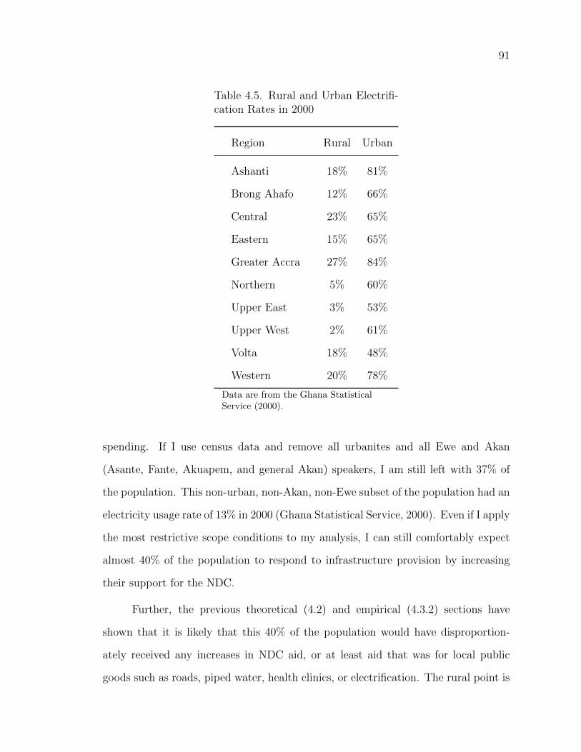
91

Table 4.5. Rural and Urban Electrifi-cation Rates in 2000

Region Rural Urban

Ashanti 18% 81%

Brong Ahafo 12% 66%

Central 23% 65%

Eastern 15% 65%

Greater Accra 27% 84%

Northern 5% 60%

Upper East 3% 53%

Upper West 2% 61%

Volta 18% 48%

Western 20% 78%

Data are from the Ghana StatisticalService (2000).

spending. If I use census data and remove all urbanites and all Ewe and Akan

(Asante, Fante, Akuapem, and general Akan) speakers, I am still left with 37% of

the population. This non-urban, non-Akan, non-Ewe subset of the population had an

electricity usage rate of 13% in 2000 (Ghana Statistical Service, 2000). Even if I apply

the most restrictive scope conditions to my analysis, I can still comfortably expect

almost 40% of the population to respond to infrastructure provision by increasing

their support for the NDC.

Further, the previous theoretical (4.2) and empirical (4.3.2) sections have

shown that it is likely that this 40% of the population would have disproportion-

ately received any increases in NDC aid, or at least aid that was for local public

goods such as roads, piped water, health clinics, or electrification. The rural point is

92

easy to follow, as the NDC’s policy platform was to target rural areas and it received

a great deal of support from rural areas. Ewe speakers would likely have received less

aid than one would expect from an economic calculation alone because Ewe speakers

reside primarily in the south of the NDC-committed Volta Region. Akan speakers

are dominant in the core NPP Ashanti region. So, while the analysis of the e↵ects of

aid spending only applies to about 40% of the population, it also applies to exactly

the population that would likely have received additional aid, had it been disbursed.

While there is strong evidence that infrastructure provision in 1999 helped the

NDC in 2000, it is not possible to precisely measure the expected magnitude of the

e↵ect across Ghana. In rural constituencies in Upper West and Upper East, the

NDC secured fewer votes in 2000 than it did in 1996, but its vote total was five

percentage points higher in the constituencies that were electrified (see Figure 4.4).

This may actually underestimate the likely magnitude of the e↵ect in other regions,

as the NDC was competing with the regionally popular PNC party in the north. In

most of Ghana, the election was always a two horse race between the NDC and NPP.

If we compare the vote change in the north between 1992 and 1996 with the vote

change between 1996 and the 2000 runo↵—which restricted the race to the NDC

and NPP—then the NDC received seven more percentage points of the vote in the

electrified constituencies.

The generally accepted story is that the NDC won votes with its infrastructure

projects in 1992 and 1996 (Bawumia, 1998; Herbst, 1993; Nugent, 1999, 2001, 2007;

Roberts, 1996). This paper provides empirical support for the belief that the NDC

benefited from such spending, and I believe that this is the first empirical analysis of

this often-made claim. While we cannot know precisely what would have happened

if donors had disbursed more of the aid that they committed, the NDC would very

likely have done better. While the NDC lost the runo↵ by a fairly large margin, it

93

only lost the first round by 4%, and it is di�cult to say what sort of runo↵ dynamics

would have been unleashed if the NDC were to have had the lead going into the

runo↵. Before the 2000 election the NDC made claims of “an anti-NDC conspiracy

by Western donors” (Gyimah-Boadi, 2001, p. 106). These claims seemed outrageous

and still seem unfounded, but they now also seem a shade closer to reality than most

donors or academics would like to admit.

4.4 Conclusion

The Ghanaian case helps to show how aid declines can harm incumbent presi-

dents. When the NDC received fewer resources from donors it was forced to cut back

on the provision of goods and services to voters. In Ghana, a large part of this was

in the form of declining developmental budget outlays for infrastructure. The NDC

had previously been popular specifically for providing infrastructure, and the places

that received new infrastructure in 1999 did vote more for the NDC than similar

places that did not receive infrastructure. Thus, the cutbacks must have hurt the

NDC.

This story of the connection between aid cuts, service provision, and ultimately

voting is a high-level form of process tracing and strongly supports the main hypoth-

esis in Chapter 2. Aid cuts hurt the NDC in 2000. The Chapter also provides support

for the main result in Chapter 3. Ghana was a well-predicted case of turnover with

a large decline in aid. It was possible that this was a spurious correlation, and while

that still could be the case, it is much less likely now that we can actually trace

causation from aid changes to projects to vote changes within Ghana. Finally, this

Chapter supports the idea that aid recipient politicians can control aid flows and

direct them according to a political logic. I was not able to measure the electoral

e↵ect of this control, but if we assume that politicians are competent and want to win

94

elections, then it follows that if they have more control over aid then they can better

improve their odds of winning elections. Finally, the Ghanaian case shows the impor-

tance of using case-specific understandings of the political landscape that politicians

face. The unique political landscape of Ghana, with two regions in the country being

strongly committed to the major parties, prevents a swing- or core-voter model from

being straightforwardly applied to the Ghanaian case. The Ghanaian government

did not favour core voters (in Volta), but instead favoured leaning swing voters or

its ‘uncommitted base.’ I will continue with this country-specific approach to un-

derstanding the electoral landscape in the remaining case study Chapters. The next

Chapter, Malawi, asks if and how President Bakili Muluzi was able to use Malawi’s

large increase in aid (about 5% of GDP) to help him win Malawi’s 1999 election.

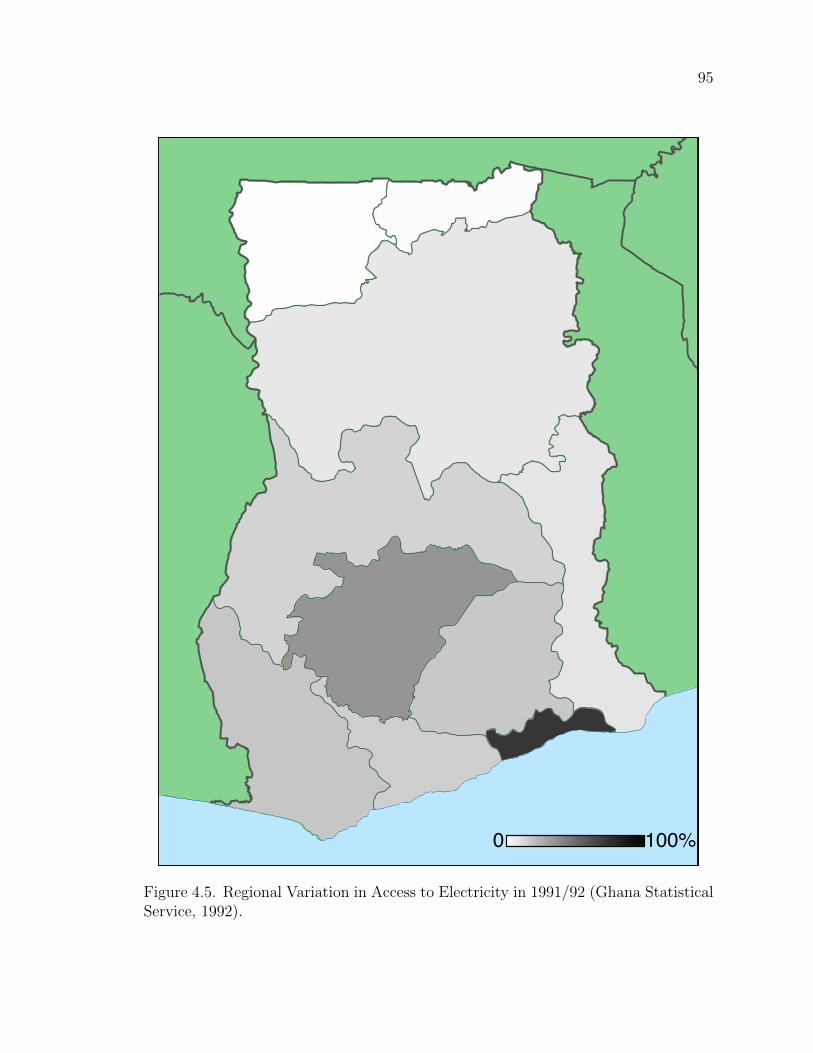
95

0 100%

Figure 4.5. Regional Variation in Access to Electricity in 1991/92 (Ghana StatisticalService, 1992).

96

CHAPTER 5

MALAWI

When Baliki Muluzi and his United Democratic Front (UDF) party won Malawi’s

first multiparty election in 1994, he took the helm of a government that was barely

functioning. Nowhere was this more true than in the education sector. In 1994,

Malawi had a primary education enrollment rate of 67%. Worse, the two-thirds of

Malawian children who were enrolled were part of a dysfunctional system with a

“20% repetition rate and 20% survival rate. On average it took learners 15 years to

complete an 8 year primary education cycle” (World Bank, 2001, p. 2). Upon being

elected in 1994, Muluzi quickly announced that he was abolishing school fees. As a

result, over a million new students entered the education system. This increased ex-

acerbated“the already acute shortages of qualitative education resource inputs such

as instructional materials, qualified teachers, opportunities for teacher professional

support and development, and increased the shortfall in teaching space to about

38,000 classrooms” (World Bank, 2001, p. 2).

It took some years, but donors responded to Malawi’s elections and Muluzi’s

move of abolishing school fees with an increase in aid. Before Muluzi’s second elec-

tion, in 1999, aid to education increased dramatically. There was a similar increase

in aid to social funds, such as the Malawi Social Action Fund (MASAF). This chap-

ter shows that political calculations influenced the allocation of some of these aid

97

projects. It also shows that voters responded to improvements in local public goods

such as education (section 5.4) or MASAF-funded road construction (section 5.3)

by increasing their vote for Muluzi. The chapter also analyzes private goods, and

section 5.5 examines a corruption scandal around procurement contracts for school

construction. It shows how the 1999 election fueled corruption in 1998 and made

donor-funded aid projects far less successful than they otherwise could have been.

The chapter also shows that it is likely that these stolen resources ended up being

used in UDF campaigns in 1999.

The Malawian case is well-predicted by the theory in chapter 2 and the re-

gressions in chapter 3. In 1998, Malawi’s saw a large increase in foreign aid. This

aid helped Muluzi win in 1999. As in the Ghanaian case, this chapter traces out

the processes linking increases in aid to increases in votes for the incumbent. This

should again increase our confidence in applying a causal interpretation to the re-

gression results in chapter 3. The Malawi chapter di↵ers from the Ghanaian in that

it traces out far more processes linking aid to votes. Aid boosted the provision of

local public goods like roads and education, and these increases helped Muluzi at the

polls in 1999. Aid was also stolen and used to influence voters before the election.

Before examining the mechanisms in more detail, I first explain the political history

of Malawi in the 1990s and then describe the role of aid in Malawi’s economic and

political development.

5.1 General political history leading up to 1999 election

After almost three decades of authoritarian rule, Malawi returned to a plural-

istic political system with the May 17, 1994 election of Baliki Muluzi of the UDF

party.1 This followed the successful referendum to repeal section 4 of the 1966 Con-

1This section draws on Chinsinga (2003) and Posner (1995).

98

stitution on June 14, 1994. Section 4 had previously made the MCP Malawi’s only

legitimate political organization.

The shift to Muluzi initially brought improved economic performance, “but

towards the end of the 1990s it rapidly deteriorated as the government faced the

prospect of securing re-election” (Cammack and Kelsall, 2011, p. 91).2 Corruption

increased dramatically in this time period, and Muluzi “oversaw the siphoning of

funds from government co↵ers by senior party people for political and personal ends”

(Cammack and Kelsall, 2011, p. 91). After the 1994 election the situation improved

briefly before declining again. Between 1997 and 2004, GNP per capita declined

from $166 to $160, and from 1996 to 2005 “Malawi experienced a high level of

macroeconomic instability due in large part to fiscal mismanagement” (World Bank,

2006, p. x). Cammack and Kelsall (2011) see di↵erences between Banda’s and

Muluzi’s rent seeking, where Banda’s was more centralized and aimed at long-term

goals and Muluzi’s was more short-term, decentralized, and damaging to rational

policy making and economic growth. TheWorld Bank saw less of a di↵erence between

the rule of Banda and Muluzi:

“The political situation during the first 10 years of the post-Banda era was stillcharacterized by power centralized in the o�ce of the president, with decision-making highly influenced by patronage and entrenched, elitist interests. Gover-nance has been poor throughout the Muluzi period (1994–2004)” (World Bank,2006, p. 2).

5.1.1 History of Malawian fiscal policy and the influence of aid

In the 1980s, Malawi was highly dependent on foreign resources and foreign

donors were more than bystanders in Malawi’s politics. The clearest example of this

is how Malawi’s authoritarian regime under Banda su↵ered from the end of the Cold

War and a newly critical donor environment. While donors had “supported Malawi

2This was common in Malawi, as “there was also a breakdown in fiscal and monetary disci-pline during the 1994 election” (World Bank, 2000b, p. 7).

99

staunchly during the Cold War years,” once it ended donors “had become critical”

and “all aid, except that of a humanitarian nature, had been suspended. That

may be the major reason for the MCP’s U-turn” (Van Donge, 1995, p. 231). The

suspension of aid, and IMF and World Bank restructuring, “disrupted in significant

ways the system for channelling rents that had [previously] worked, with limitations,

under Banda.” (Cammack and Kelsall, 2011, p. 91). After the 1994 election, aid

increased again. Throughout this time, the Malawian government relied on donors

to fund much of its development budget.

Figure 5.1 shows the close relationship between foreign grants and Malawian

development expenditure (r=0.997).3 This correlation holds over the entire period

before the election, including when aid increased dramatically in fiscal years 1998/99

and 1999/2000. The tight fit between grants and development spending highlights

the extent to which Malawi’s capital budget was reliant on foreign funding. Malawi,

in fact, was one of the most aid dependent countries in the world, and “in 1997

external grants and borrowings were equivalent to 10 percent of GDP and 40 percent

of government expenditure, Malawi’s external debt was about $2.6 billion, equivalent

to 107 percent of GDP” (World Bank, 2006, p. 3). From that point, Malawi’s aid

dependence actually increased and by 2000, its external debt was at 140 percent

of GDP (World Bank, 2006). Net ODA during 1998 to 2004 averaged about $450

million per year (World Bank, 2006).

Figure 5.1 shows that aid to Malawi dramatically increased in the late 1990s.

This is evident in the OECD’s ODA figures and in Malawian government data. In

1998, the Malawian government described the situation thusly:

3The correlation between net loans and developmental spending in the same time periodis 0.66, but this reduction is due to the final year when repayments increased. Over the period1994/95 to 1998/99, the correlation between net loans and developmental spending is 0.97. Thedata come from the Government of Malawi’s National Economic Council’s Economic Reports. Thegraph shows actual figures.

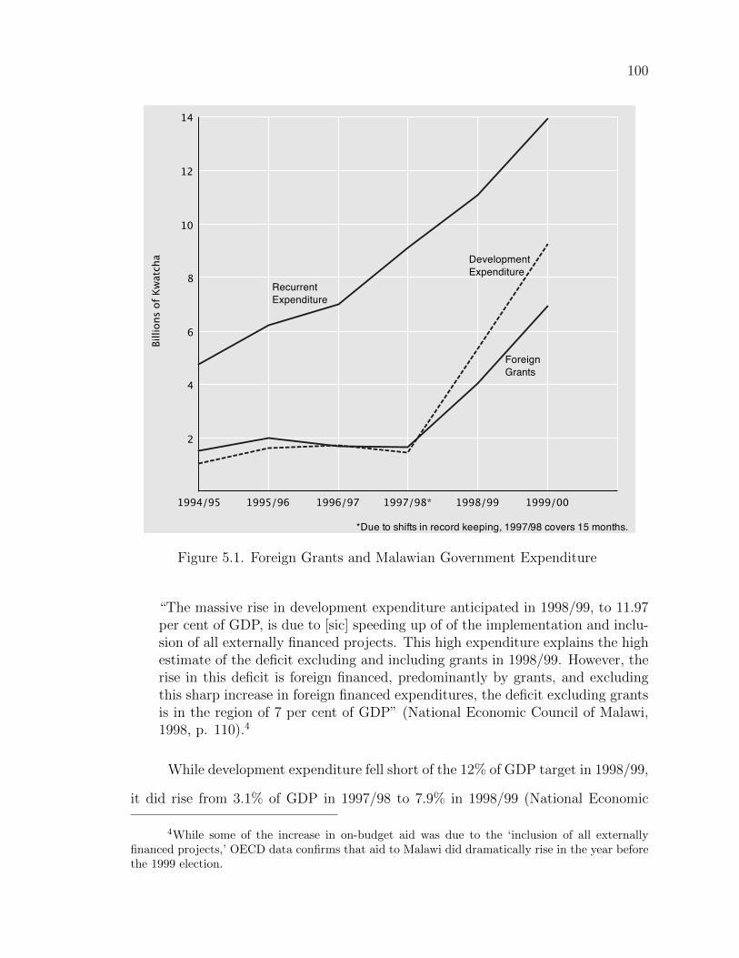
100

1994/95 1995/96 1996/97 1997/98* 1998/99 1999/00

14

2

4

6

8

10

12

Billi

ons

of K

wat

cha

*Due to shifts in record keeping, 1997/98 covers 15 months.

ForeignGrants

DevelopmentExpenditure

RecurrentExpenditure

Figure 5.1. Foreign Grants and Malawian Government Expenditure

“The massive rise in development expenditure anticipated in 1998/99, to 11.97per cent of GDP, is due to [sic] speeding up of of the implementation and inclu-sion of all externally financed projects. This high expenditure explains the highestimate of the deficit excluding and including grants in 1998/99. However, therise in this deficit is foreign financed, predominantly by grants, and excludingthis sharp increase in foreign financed expenditures, the deficit excluding grantsis in the region of 7 per cent of GDP” (National Economic Council of Malawi,1998, p. 110).4

While development expenditure fell short of the 12% of GDP target in 1998/99,

it did rise from 3.1% of GDP in 1997/98 to 7.9% in 1998/99 (National Economic

4While some of the increase in on-budget aid was due to the ‘inclusion of all externallyfinanced projects,’ OECD data confirms that aid to Malawi did dramatically rise in the year beforethe 1999 election.

101

Council of Malawi, 2000, p. 114). The government economic reports are crystal

clear on the source of this increase: “this massive rise in development expenditure

over previous levels can be predominantly explained by a surge in donor funded

development projects” (National Economic Council of Malawi, 1998, p. 116). As

was noted in the closing portion of Chapter 3, about half of this increase was due

to the EC and about half was due to smaller increases on the part of other donors.

There is no evidence that the aid increase had anything to do with the 1999 election.

The timing of the increase seems to be largely due to luck. The next section describes

the voting patterns in Malawi’s 1994 and 1999 elections and then the remainder of

the Chapter examines if the aid increase in 1998 helped Muluzi win the election in

1999.

5.1.2 The 1999 Election

Voting patterns in Malawi’s 1994 and 1999 elections were distinctly regional

and quite static. During this time Southern region was the UDF’s territory, the

MCP was dominant in Central region, and the Alliance for Democracy (AFORD)

controlled Northern region. The seat breakdowns for the two elections are shown in

Tables 5.1 and 5.2. While Malawi’s party system had some shifts between elections,

Malawi’s regions tended to vote in blocs until 2009 (Ferree and Horowitz, 2010).

Presidential voting showed a similarly pronounced, fixed regional pattern in

both elections. The correlation between district-level presidential vote returns in

1994 and 1999 is very high (at r=0.98).5 Despite the voting similarities, Muluzi

managed to increase his share of the vote from 47% in 1994 to 52% in 1999 (Van

Donge, 1995; Economist Intelligence Unit, 1999). Greater variation in district-level

voting changes between 1994 and 1999 would have simplified an analysis of the e↵ect

5Two new districts in Southern region were created in 1998. These were dropped from the1999 elections in order to make this comparison possible.

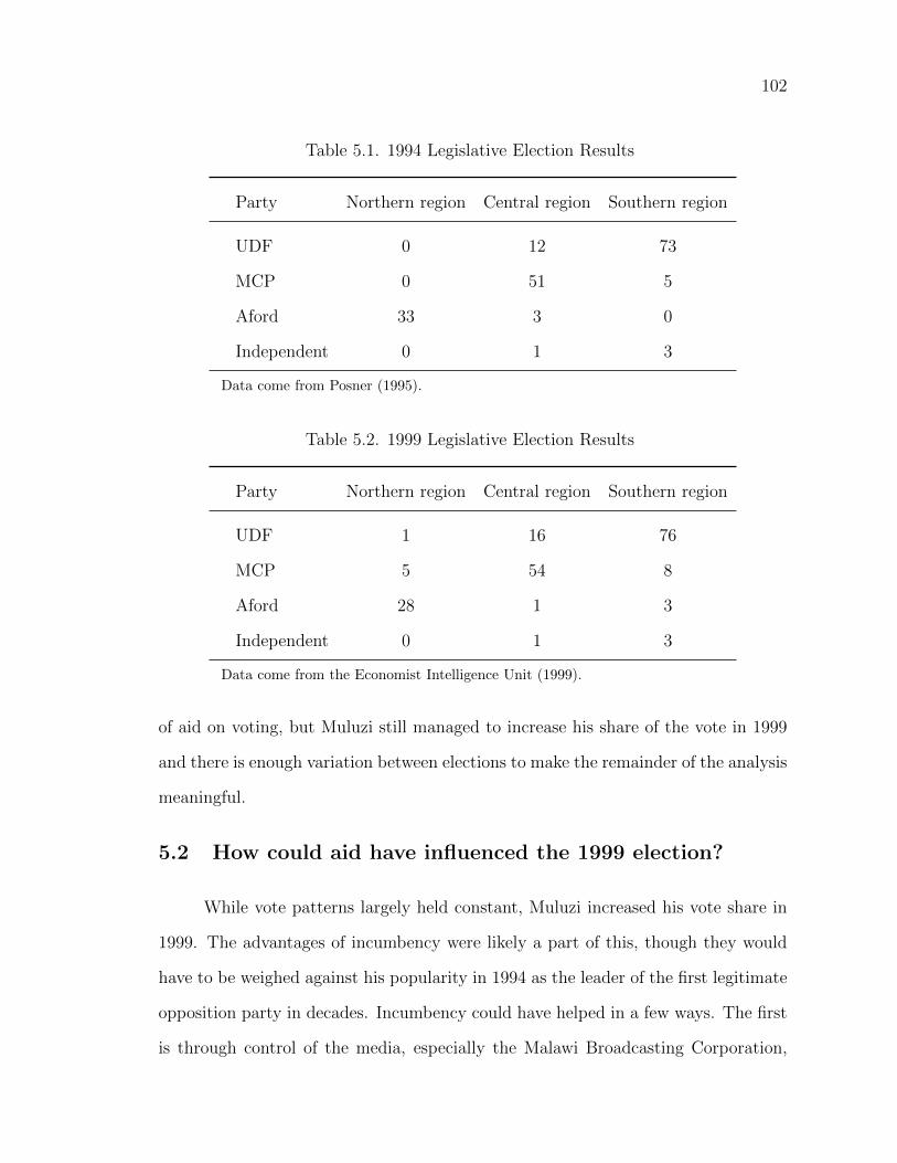
102

Table 5.1. 1994 Legislative Election Results

Party Northern region Central region Southern region

UDF 0 12 73

MCP 0 51 5

Aford 33 3 0

Independent 0 1 3

Data come from Posner (1995).

Table 5.2. 1999 Legislative Election Results

Party Northern region Central region Southern region

UDF 1 16 76

MCP 5 54 8

Aford 28 1 3

Independent 0 1 3

Data come from the Economist Intelligence Unit (1999).

of aid on voting, but Muluzi still managed to increase his share of the vote in 1999

and there is enough variation between elections to make the remainder of the analysis

meaningful.

5.2 How could aid have influenced the 1999 election?

While vote patterns largely held constant, Muluzi increased his vote share in

1999. The advantages of incumbency were likely a part of this, though they would

have to be weighed against his popularity in 1994 as the leader of the first legitimate

opposition party in decades. Incumbency could have helped in a few ways. The first

is through control of the media, especially the Malawi Broadcasting Corporation,

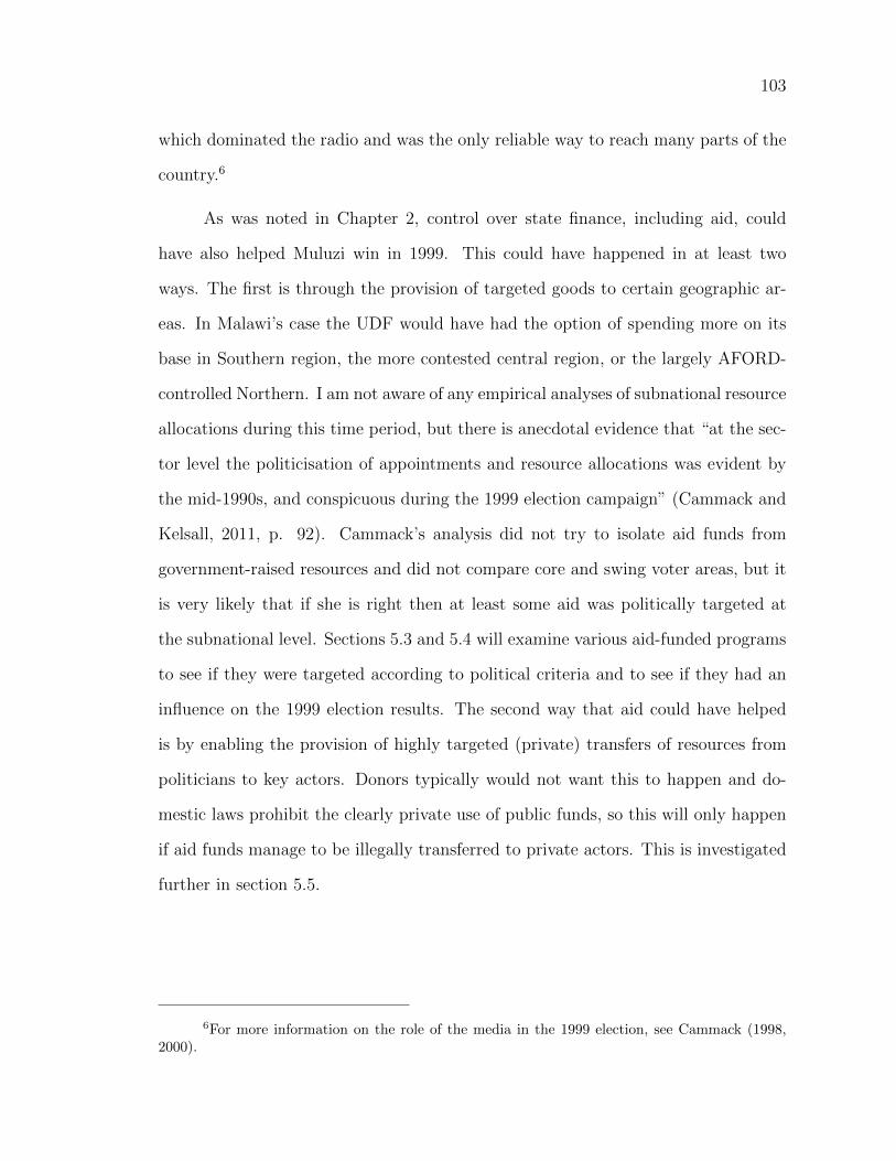
103

which dominated the radio and was the only reliable way to reach many parts of the

country.6

As was noted in Chapter 2, control over state finance, including aid, could

have also helped Muluzi win in 1999. This could have happened in at least two

ways. The first is through the provision of targeted goods to certain geographic ar-

eas. In Malawi’s case the UDF would have had the option of spending more on its

base in Southern region, the more contested central region, or the largely AFORD-

controlled Northern. I am not aware of any empirical analyses of subnational resource

allocations during this time period, but there is anecdotal evidence that “at the sec-

tor level the politicisation of appointments and resource allocations was evident by

the mid-1990s, and conspicuous during the 1999 election campaign” (Cammack and

Kelsall, 2011, p. 92). Cammack’s analysis did not try to isolate aid funds from

government-raised resources and did not compare core and swing voter areas, but it

is very likely that if she is right then at least some aid was politically targeted at

the subnational level. Sections 5.3 and 5.4 will examine various aid-funded programs

to see if they were targeted according to political criteria and to see if they had an

influence on the 1999 election results. The second way that aid could have helped

is by enabling the provision of highly targeted (private) transfers of resources from

politicians to key actors. Donors typically would not want this to happen and do-

mestic laws prohibit the clearly private use of public funds, so this will only happen

if aid funds manage to be illegally transferred to private actors. This is investigated

further in section 5.5.

6For more information on the role of the media in the 1999 election, see Cammack (1998,2000).

104

5.2.1 Where would Muluzi target aid?

Unlike Ghana, Malawi did not have fully committed regions. While Muluzi’s

UDF party dominated the South of the country and was far less popular in the

Center and the North, these patterns were the result of genuine di↵erences in the

perception of the government and not primarily the result of expressive motivations7

or identity (Ferree and Horowitz, 2010). In this situation, with no committed areas,

it seems likely that Muluzi’s strategy would be to target voters that leaned towards

his party, and usually resided in the South.

Malawi experienced a large aid increase before the 1999 election. The challenge

is to examine if this aid influenced votes for Muluzi and how the change in aid may

have been linked to votes. I have general budget information, which confirms an

aid increase and shows roughly where that aid was spent. I am interested in three

large aid projects: education construction, MASAF, and the fertilizer subsidy. I have

fairly good information on education construction and MASAF, but neither dataset

is perfect.8

5.3 Malawi Social Action Fund

MASAF is a decentralized social fund that was explicitly set up to be at arms-

length from the government. I will first examine the degree to which politics seems

to have influenced MASAF allocations and then I will examine the degree to which

7Expressive ethnic voters use voting as an opportunity to demonstrate their membership inan ethnic group. For more on expressive ethnic voting see (Horowitz, 1985).

8I lack information on the fertilizer subsidy program in 1998. Probably the most importantaid-funded initiative during this time was the ‘Starter Pack’ fertilizer subsidy program. Unfortu-nately, after extensive searching I was only able to build a dataset of fertilizer allocations from1999–2004. I found reports from 1998, the first year of the subsidy, but these reports lacked thedetailed statistical appendices that follow all of the other reports. Without these appendices Icannot judge who received the subsidy and if it had any e↵ect on the 1999 election.

105

MASAF allocations seemed to have helped Muluzi.9

MASAF was created in 1995 and funded by the World Bank and the Govern-

ment of Malawi. This was a large part of Malawi’s antipoverty strategy, and received

a great deal of political support. “The President attended the launches of the pilot

project and the full project. He made many speeches in support of MASAF” (Bloom,

2003, p. 62). The president also “eventually moved the project into the O�ce of the

President and Cabinet” (Bloom, 2003, p. 62). MASAF estimates that it provided

assistance to over 5 million people between 1996 and 2005 (World Bank, 2006, p.

xi).

MASAF funded two types of projects: community service projects (CSP) and

larger public works projects (PWP). Communities had to apply to MASAF with

a proposal for a CSP.10 This process started with the community electing a man-

agement committee which drafted a plan for the project. In a community’s plan

had to specify how they planned to meet MASAF’s 20% cost-sharing requirement.

This was usually met through o↵ering labour at the local minimum wage, though

sometimes materials were also o↵ered. Once the plan was finalized it was vetted

by the District Executive Committee (DEC), which is composed of o�cers of the

line ministries operating at the district level. So, if a project relates to health it

will receive more scrutiny from the district health o�cer. After DEC approval, the

project passed to the MASAF management unit in Lilongwe. MASAF—like other

social funds—is administered by a management unit that is formally independent of

the central government. If the management unit approves the project then it passes

to the MASAF steering committee. This is the one stage of the process where “the

9Muluzi frequently referred to MASAF as his program and was quick to reference it whilecampaigning. While this symbolic use of MASAF may have helped Muluzi, I focus instead on moremeasurable e↵ects of actual spending in districts.

10This summary is drawn from a more extensive overview by Schroeder (2000).

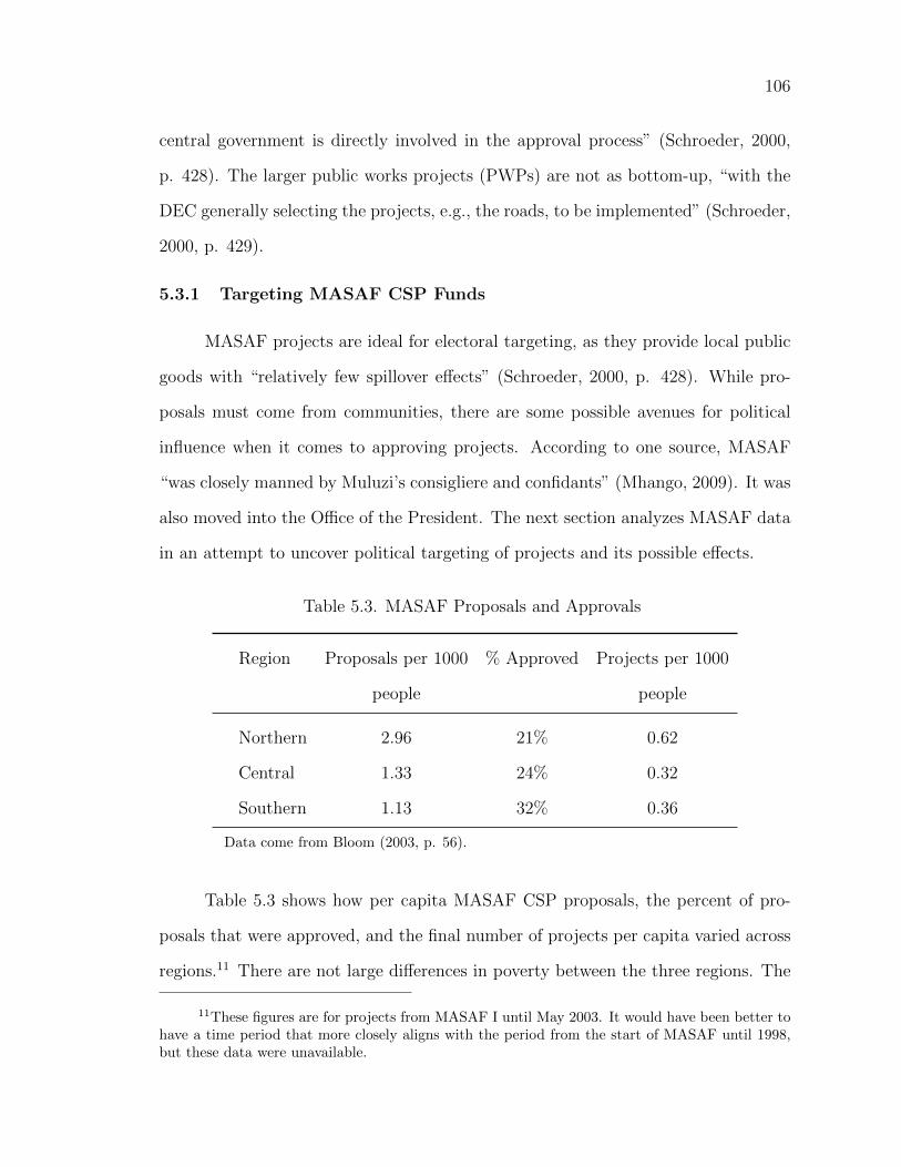
106

central government is directly involved in the approval process” (Schroeder, 2000,

p. 428). The larger public works projects (PWPs) are not as bottom-up, “with the

DEC generally selecting the projects, e.g., the roads, to be implemented” (Schroeder,

2000, p. 429).

5.3.1 Targeting MASAF CSP Funds

MASAF projects are ideal for electoral targeting, as they provide local public

goods with “relatively few spillover e↵ects” (Schroeder, 2000, p. 428). While pro-

posals must come from communities, there are some possible avenues for political

influence when it comes to approving projects. According to one source, MASAF

“was closely manned by Muluzi’s consigliere and confidants” (Mhango, 2009). It was

also moved into the O�ce of the President. The next section analyzes MASAF data

in an attempt to uncover political targeting of projects and its possible e↵ects.

Table 5.3. MASAF Proposals and Approvals

Region Proposals per 1000 % Approved Projects per 1000

people people

Northern 2.96 21% 0.62

Central 1.33 24% 0.32

Southern 1.13 32% 0.36

Data come from Bloom (2003, p. 56).

Table 5.3 shows how per capita MASAF CSP proposals, the percent of pro-

posals that were approved, and the final number of projects per capita varied across

regions.11 There are not large di↵erences in poverty between the three regions. The

11These figures are for projects from MASAF I until May 2003. It would have been better tohave a time period that more closely aligns with the period from the start of MASAF until 1998,but these data were unavailable.

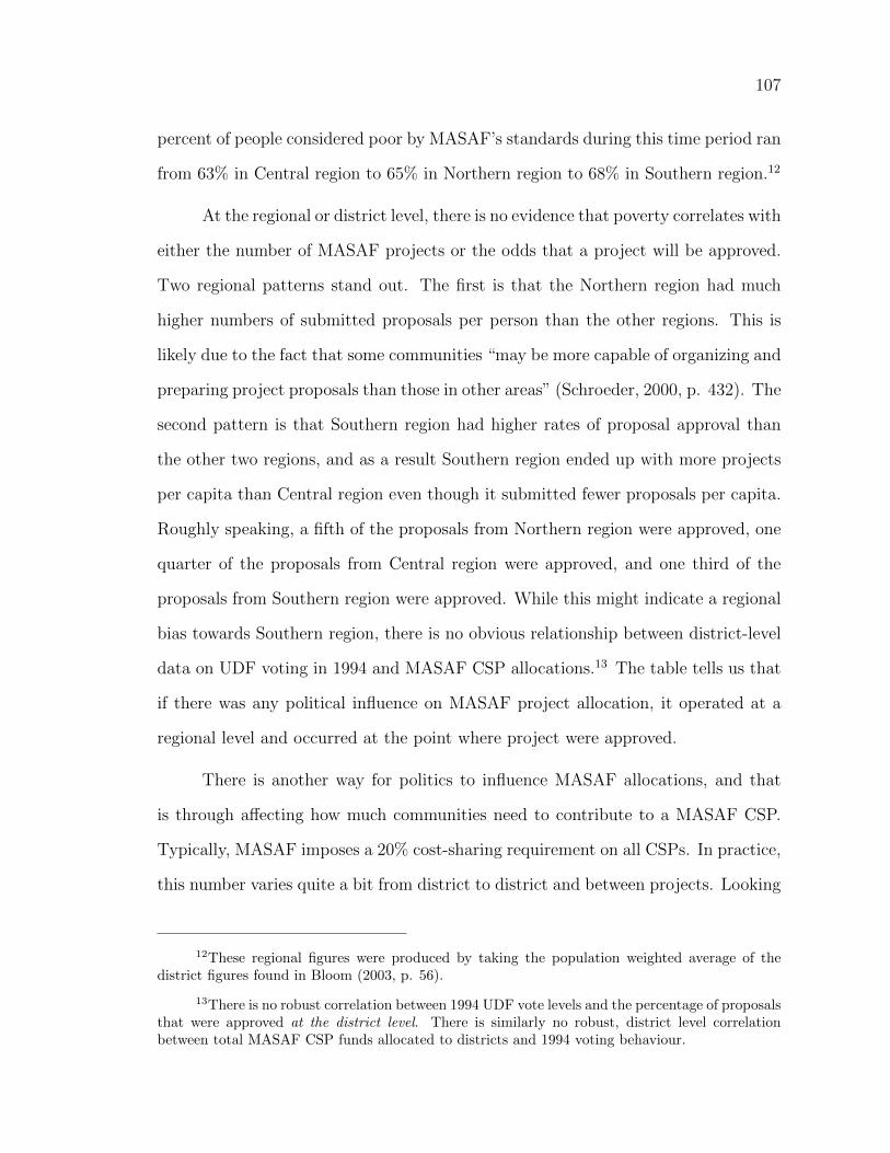
107

percent of people considered poor by MASAF’s standards during this time period ran

from 63% in Central region to 65% in Northern region to 68% in Southern region.12

At the regional or district level, there is no evidence that poverty correlates with

either the number of MASAF projects or the odds that a project will be approved.

Two regional patterns stand out. The first is that the Northern region had much

higher numbers of submitted proposals per person than the other regions. This is

likely due to the fact that some communities “may be more capable of organizing and

preparing project proposals than those in other areas” (Schroeder, 2000, p. 432). The

second pattern is that Southern region had higher rates of proposal approval than

the other two regions, and as a result Southern region ended up with more projects

per capita than Central region even though it submitted fewer proposals per capita.

Roughly speaking, a fifth of the proposals from Northern region were approved, one

quarter of the proposals from Central region were approved, and one third of the

proposals from Southern region were approved. While this might indicate a regional

bias towards Southern region, there is no obvious relationship between district-level

data on UDF voting in 1994 and MASAF CSP allocations.13 The table tells us that

if there was any political influence on MASAF project allocation, it operated at a

regional level and occurred at the point where project were approved.

There is another way for politics to influence MASAF allocations, and that

is through a↵ecting how much communities need to contribute to a MASAF CSP.

Typically, MASAF imposes a 20% cost-sharing requirement on all CSPs. In practice,

this number varies quite a bit from district to district and between projects. Looking

12These regional figures were produced by taking the population weighted average of thedistrict figures found in Bloom (2003, p. 56).

13There is no robust correlation between 1994 UDF vote levels and the percentage of proposalsthat were approved at the district level. There is similarly no robust, district level correlationbetween total MASAF CSP funds allocated to districts and 1994 voting behaviour.

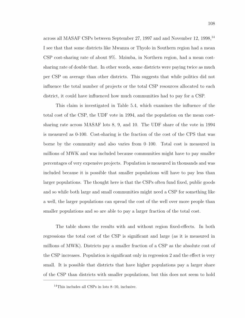
108

across all MASAF CSPs between September 27, 1997 and and November 12, 1998,14

I see that that some districts like Mwanza or Thyolo in Southern region had a mean

CSP cost-sharing rate of about 9%. Mzimba, in Northern region, had a mean cost-

sharing rate of double that. In other words, some districts were paying twice as much

per CSP on average than other districts. This suggests that while politics did not

influence the total number of projects or the total CSP resources allocated to each

district, it could have influenced how much communities had to pay for a CSP.

This claim is investigated in Table 5.4, which examines the influence of the

total cost of the CSP, the UDF vote in 1994, and the population on the mean cost-

sharing rate across MASAF lots 8, 9, and 10. The UDF share of the vote in 1994

is measured as 0-100. Cost-sharing is the fraction of the cost of the CPS that was

borne by the community and also varies from 0–100. Total cost is measured in

millions of MWK and was included because communities might have to pay smaller

percentages of very expensive projects. Population is measured in thousands and was

included because it is possible that smaller populations will have to pay less than

larger populations. The thought here is that the CSPs often fund fixed, public goods

and so while both large and small communities might need a CSP for something like

a well, the larger populations can spread the cost of the well over more people than

smaller populations and so are able to pay a larger fraction of the total cost.

The table shows the results with and without region fixed-e↵ects. In both

regressions the total cost of the CSP is significant and large (as it is measured in

millions of MWK). Districts pay a smaller fraction of a CSP as the absolute cost of

the CSP increases. Population is significant only in regression 2 and the e↵ect is very

small. It is possible that districts that have higher populations pay a larger share

of the CSP than districts with smaller populations, but this does not seem to hold

14This includes all CSPs in lots 8–10, inclusive.

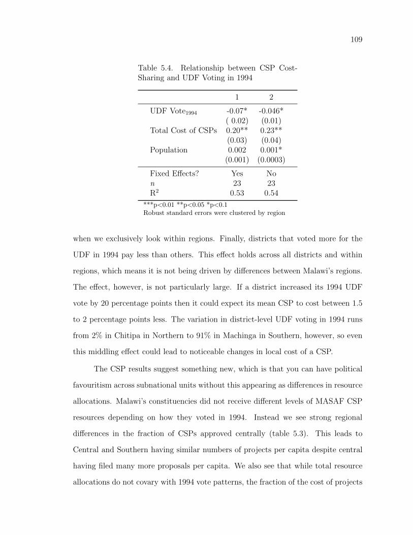
109

Table 5.4. Relationship between CSP Cost-Sharing and UDF Voting in 1994

1 2

UDF Vote1994 -0.07* -0.046*( 0.02) (0.01)

Total Cost of CSPs 0.20** 0.23**(0.03) (0.04)

Population 0.002 0.001*(0.001) (0.0003)

Fixed E↵ects? Yes Non 23 23R2 0.53 0.54

***p<0.01 **p<0.05 *p<0.1Robust standard errors were clustered by region

when we exclusively look within regions. Finally, districts that voted more for the

UDF in 1994 pay less than others. This e↵ect holds across all districts and within

regions, which means it is not being driven by di↵erences between Malawi’s regions.

The e↵ect, however, is not particularly large. If a district increased its 1994 UDF

vote by 20 percentage points then it could expect its mean CSP to cost between 1.5

to 2 percentage points less. The variation in district-level UDF voting in 1994 runs

from 2% in Chitipa in Northern to 91% in Machinga in Southern, however, so even

this middling e↵ect could lead to noticeable changes in local cost of a CSP.

The CSP results suggest something new, which is that you can have political

favouritism across subnational units without this appearing as di↵erences in resource

allocations. Malawi’s constituencies did not receive di↵erent levels of MASAF CSP

resources depending on how they voted in 1994. Instead we see strong regional

di↵erences in the fraction of CSPs approved centrally (table 5.3). This leads to

Central and Southern having similar numbers of projects per capita despite central

having filed many more proposals per capita. We also see that while total resource

allocations do not covary with 1994 vote patterns, the fraction of the cost of projects

110

that must be borne locally is smaller in the constituencies that voted more for the

UDF in 1994 (5.4). This pattern holds with region fixed-e↵ects, showing that it is

not regional in origin. This indicates a channel of targeting that is distinct from

favouring communities with more total resources, as happened with electrification in

Ghana. This form of targeting will not be active in most other forms of resources, as

it likely grows from the partially-arms-length nature of the MASAF CSP process. If

all decisions are made centrally, as they were with the MASAF PWPs, then I expect

that favoritism will show up in the standard form of more resources in places that

are targeted.

5.3.2 Targeting MASAF PWP Funds

There are three ways that PWPs are di↵erent from CSPs. First, while CSP

allocations were driven by community demand, PWPs were selected centrally. Sec-

ond, while CSPs and PWPs were aimed at alleviating poverty, only the larger PWPs

explicitly built in a strategy of alleviating poverty through hiring local people to

work on the PWP.15 Third, resources for PWPs comes wholly from MASAF instead

of being partially sourced locally. About 86% of all PWPs were for the construction

of roads (Malawi Social Action Fund, 1999), and I examine only road funds.16

The regression results reported in Table 5.5 show how voting and population

covary with PWP road resources. PWP funds are measured per square kilometer.

Population is insignificant. The p-value for the vote share in the first regression is

0.052. Adding region fixed-e↵ects reduces the influence of the UDF vote in 1994

to p=0.141. The specification used in both regressions explains only 14% of the

15From the 1999 MASAF Factfile: “The objective of the PWP is to create employmentopportunities for income transfer and in the process build economic infrastructure through labourintensive activities” (Malawi Social Action Fund, 1998, p. 53).

1611% were for a↵orestation and 3% were for water related projects.

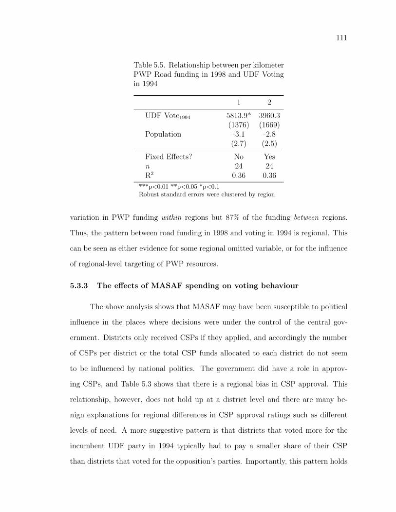
111

Table 5.5. Relationship between per kilometerPWP Road funding in 1998 and UDF Votingin 1994

1 2

UDF Vote1994 5813.9* 3960.3(1376) (1669)

Population -3.1 -2.8(2.7) (2.5)

Fixed E↵ects? No Yesn 24 24R2 0.36 0.36

***p<0.01 **p<0.05 *p<0.1Robust standard errors were clustered by region

variation in PWP funding within regions but 87% of the funding between regions.

Thus, the pattern between road funding in 1998 and voting in 1994 is regional. This

can be seen as either evidence for some regional omitted variable, or for the influence

of regional-level targeting of PWP resources.

5.3.3 The e↵ects of MASAF spending on voting behaviour

The above analysis shows that MASAF may have been susceptible to political

influence in the places where decisions were under the control of the central gov-

ernment. Districts only received CSPs if they applied, and accordingly the number

of CSPs per district or the total CSP funds allocated to each district do not seem

to be influenced by national politics. The government did have a role in approv-

ing CSPs, and Table 5.3 shows that there is a regional bias in CSP approval. This

relationship, however, does not hold up at a district level and there are many be-

nign explanations for regional di↵erences in CSP approval ratings such as di↵erent

levels of need. A more suggestive pattern is that districts that voted more for the

incumbent UDF party in 1994 typically had to pay a smaller share of their CSP

than districts that voted for the opposition’s parties. Importantly, this pattern holds

112

both across Malawi and between districts in each of Malawi’s regions. The PWP

results caution against a strong view that the central government exerted control

over funding outcomes. While the government ostensibly exercised more power over

fully-centralized decision making, PWP road spending is not significantly related to

UDF voting within regions. As with the approval rates for CSPs, if there is political

bias then it appears to mostly work at a regional level.

However, while the above analyses show the points where the government could

control funds, it does not show that the government benefited from this control.

Three points here are important. First, MASAF was quite a popular program across

Malawi and every district received MASAF projects. If MASAF was seen more as

an important national program instead of a district-level transfer, then it could have

helped the government gain votes without showing a district-level pattern. This

would be a good example of the symbolic power of an aid program (see section

2.2.3). Second, while the government was able to exert control over some portions

of MASAF, many of the most important aspects of MASAF, such as total funds

allocated to a district or the number of projects per district, were not influenced

by national politics. Third, no MASAF CSP variable for which I have data exerts

a significant influence on vote percentages for the UDF in 1999 when I add basic

control variables such as the percentage of the vote for the UDF in 1994. This is

not the case, however, for the PWPs. Voters seem to be more influenced by large

projects such as road construction and far less by smaller CSP projects such as the

drilling of wells.

Table 5.6 shows how PWP funding from di↵erent time periods (measured in

thousands of MWK per km2) relates to UDF vote levels in 1999 and figure 5.2 shows

how PWP road aid was distributed across Malawi. I control for UDF vote levels

in 1994 and add region fixed e↵ects. The main result from table 5.6 is that voters

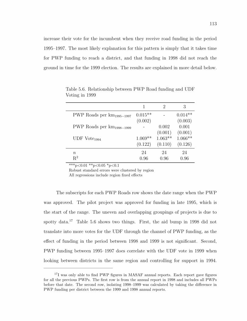
113

increase their vote for the incumbent when they receive road funding in the period

1995–1997. The most likely explanation for this pattern is simply that it takes time

for PWP funding to reach a district, and that funding in 1998 did not reach the

ground in time for the 1999 election. The results are explained in more detail below.

Table 5.6. Relationship between PWP Road funding and UDFVoting in 1999

1 2 3

PWP Roads per km1995�1997 0.015** - 0.014**(0.002) (0.003)

PWP Roads per km1998�1999 - 0.002 0.001(0.001) (0.001)

UDF Vote1994 1.069** 1.063** 1.066**(0.122) (0.110) (0.126)

n 24 24 24R2 0.96 0.96 0.96

***p<0.01 **p<0.05 *p<0.1Robust standard errors were clustered by regionAll regressions include region fixed e↵ects

The subscripts for each PWP Roads row shows the date range when the PWP

was approved. The pilot project was approved for funding in late 1995, which is

the start of the range. The uneven and overlapping groupings of projects is due to

spotty data.17 Table 5.6 shows two things. First, the aid bump in 1998 did not

translate into more votes for the UDF through the channel of PWP funding, as the

e↵ect of funding in the period between 1998 and 1999 is not significant. Second,

PWP funding between 1995–1997 does correlate with the UDF vote in 1999 when

looking between districts in the same region and controlling for support in 1994.

17I was only able to find PWP figures in MASAF annual reports. Each report gave figuresfor all the previous PWPs. The first row is from the annual report in 1998 and includes all PWPsbefore that date. The second row, isolating 1998–1999 was calculated by taking the di↵erence inPWP funding per district between the 1999 and 1998 annual reports.

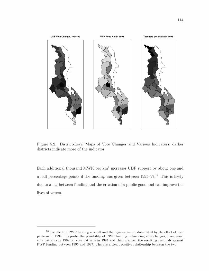
114

UDF Vote Change, 1994−99 PWP Road Aid in 1998 Teachers per capita in 1998

Figure 5.2. District-Level Maps of Vote Changes and Various Indicators, darkerdistricts indicate more of the indicator

Each additional thousand MWK per km2 increases UDF support by about one and

a half percentage points if the funding was given between 1995–97.18 This is likely

due to a lag between funding and the creation of a public good and can improve the

lives of voters.

18The e↵ect of PWP funding is small and the regressions are dominated by the e↵ect of votepatterns in 1994. To probe the possibility of PWP funding influencing vote changes, I regressedvote patterns in 1999 on vote patterns in 1994 and then graphed the resulting residuals againstPWP funding between 1995 and 1997. There is a clear, positive relationship between the two.

115

5.4 Actual Improvements in the Provision of Primary Edu-cation

Aside from MASAF, Muluzi also could have benefited from aid to education.

As was noted in the introduction, when Muluzi took power Malawi had a primary

education enrollment rate of 67%. Muluzi’s response was to abolish school fees,

which increase enrollment but stretched an already resource-poor Ministry. The

abolishment of school fees exacerbated the shortages already existing in the education

sector and “increased the shortfall in teaching space to about 38,000 classrooms”

(World Bank, 2001, p. 2).

This section has two subsections. The first evaluates if actual improvements

in teachers and schoolrooms helped Muluzi. The other examines the corruption

scandal that surrounded school construction. It is worth focusing on education for

two reasons. The first reason is because Muluzi made increasing the availably of

education across Malawi a priority for his government. The second reason is because

increasing education was very expensive19 and was helped along greatly by foreign

resources. Throughout this period, education took between about 15–25% of the

development budget, typically making it the single largest sector in each year. The

budget for 1999 notes that “the allocation of resources to the development budget for

the past three years have increased mainly due to increased pressure emerging from

construction of new schools” (National Economic Council of Malawi, 2000, p. 111).

This means that the e↵ect of education spending is critical to understanding the

e↵ect of the aid increase in Malawi, as much of the aid increase was due to increases

in aid for education. I first examine if voters were responsive to this e↵ort.

Actual improvements on education are hard to measure due to wildly varying

19More than a quarter of Malawi’s development budget was allocated to the education sectorin 1997/98 (National Economic Council of Malawi, 1998, p. 105).

116

statistics. I collected data on di↵erent measures of educational infrastructure from

the Ministry of Education and the National Statistical O�ce. There are two potential

problems with these data. First, it seems that the Ministry of Education collected

its information from the schools in each district through a survey. Unfortunately

there is no record of non-responses or information on the expected number of schools

per district. This means that I cannot know if changes in the number of responding

schools between years is the result of new schools being built or just higher response

rates. Second, I took figures for the number of classrooms in each district and then

summed them by region. When I do this I do not get the same totals as the Ministry

of Education, and I am able to isolate the problem to specific errors in arithmetic

on the part of the Ministry20. The di↵erences between my figures and the reported

totals in the Ministry’s tables are not typically larger than a few hundred, but this

discrepancy points to potentially larger problems with the data. It is known that

there was certainly a large increase in construction during this time period, but it is

di�cult to measure.

I dealt with the problem of noisy data in a few ways. One way was to analyze

di↵erent measures of educational spending and to see if they correlate. For example, I

have information on the number of teachers per district and the number of classrooms

per district. One would expect these to correlate, as the most e�cient number

of teachers per classroom is 1. There is a high correlation between teachers and

classrooms, especially in 1998. If I had good evidence that these two data sources

were independent, then this could increase our confidence in the measures. However,

I was unable to find anyone who could tell me precisely how either measure was

created, and it seems likely that they came from the same survey and so have the

same problems.

20As an example, on page 70 of Malawi Government (1999), 884+854+534+855+609 6= 4401

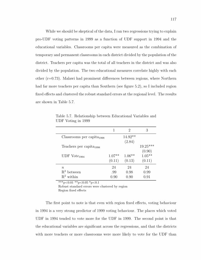
117

While we should be skeptical of the data, I ran two regressions trying to explain

pro-UDF voting patterns in 1999 as a function of UDF support in 1994 and the

educational variables. Classrooms per capita were measured as the combination of

temporary and permanent classrooms in each district divided by the population of the

district. Teachers per capita was the total of all teachers in the district and was also

divided by the population. The two educational measures correlate highly with each

other (r=0.73). Malawi had prominent di↵erences between regions, where Northern

had far more teachers per capita than Southern (see figure 5.2), so I included region

fixed e↵ects and clustered the robust standard errors at the regional level. The results

are shown in Table 5.7.

Table 5.7. Relationship between Educational Variables andUDF Voting in 1999

1 2 3

Classrooms per capita1998 14.92**(2.84)

Teachers per capita1998 19.25***(0.90)

UDF Vote1994 1.07** 1.06** 1.05**(0.11) (0.13) (0.11)

n 24 24 24R2 between .99 0.98 0.99R2 within 0.90 0.90 0.91

***p<0.01 **p<0.05 *p<0.1Robust standard errors were clustered by regionRegion fixed e↵ects

The first point to note is that even with region fixed e↵ects, voting behaviour

in 1994 is a very strong predictor of 1999 voting behaviour. The places which voted

UDF in 1994 tended to vote more for the UDF in 1999. The second point is that

the educational variables are significant across the regressions, and that the districts

with more teachers or more classrooms were more likely to vote for the UDF than

118

the districts with fewer teachers or classrooms. Given that a huge amount of the

education budget was being funded by donors, it is very likely that aid helped Muluzi

through the public goods mechanism of increasing education. The biggest problem

with this interpretation is that while the levels of teachers or classrooms in 1998 is

a statistically significant predictor of 1999 vote levels, changes in teachers or class-

rooms per capita moving from previous time periods to 1998 are not. There are two

explanations for this. First, it could be that the data are of poor quality and that

this quality is uneven over time. For example, if these figures are taken from surveys

and di↵erent numbers of schools respond each time then di↵erences in figures over

time would capture response rates as much as actual changes in the number of class-

rooms or teachers. I know of no good solution to this problem. Second, it could be

that citizens were not voting based on actual changes in educational infrastructure,

but rather on the state of education in their district in 1998. This could be possible

if voters have short memories and evaluate politicians impact on their life at one

moment before the election and not dynamically over time. If this is the case, then

the vast, donor-funded increase in education could have led to the UDF doing better

in the 1999 election.

5.5 Corruption surrounding school construction

There is one final way that donor funding for education could have helped the

UDF win the 1999 election, and this is through corruption. When the Malawian

government eliminated school fees it saw a very large in increase in the number

of students. The school system was not built to handle such a large number of

students, and in order to meet the demand for education the government engaged

in country-wide school construction. Meeting the demand for free education also

required the mass hiring and training of teachers and the purchase of educational

119

materials. A large portion of the resources for the extension of education came from

foreign donors, and as the previous section has shown, voters seemed to appreciate

higher levels of teachers or classrooms in their district. However, the construction

and buying boom also facilitated a great deal of corruption. The Auditor General’s

report of 2001 stated:

“Between 2000 and 2001, I issued five reports and one special report on man-agement public works contractors in the Ministry of Education, Science andTechnology. The reports highlighted serious weaknesses in dubious awarding ofcontracts to Contractors to build school blocks, failure to monitor the construc-tion works and wrong payments to contractors” (Kalongonda, 2002, p. 157).

These weakness led to at least 187 million kwatcha (approx. 6 million 1998

USD) going to contractors who had either not carried out their work, abandoned their

work, or overcharged for the work done (Kalongonda, 2002, p. 157). There were sim-

ilar problems surrounding the procurement of educational materials between 1998

and 2000. In this case, o�cers had signed o↵ on textbooks and other educational

materials having been received even though they were not in storehouses. They were

never recovered. The value of this loss was estimated at about 120 million kwatcha

(Kalongonda, 2002, p. 157). Between 1998 and 1999, another 10 million kwatcha

worth of additional educational materials were removed from storehouses through

a voucher scam. All of the O�cers implicated in these scandals continued to work

for the government. Between December 1996 and February 2000, about 11.5 million

kwatcha worth of contracts for educational materials were paid to contractors who

failed to fulfill the contract. The contractors kept the cash.21 Finally, between June

1998 and December 1999, another 11.5 million kwatcha were over-billed to the gov-

ernment due to contractors falsely claiming that they bought supplies overseas when

21The audit report is not clear on this point, but it appears that these contractors were paidin advance of the completion of the contact. This occurred with other scams in the EducationMinistry, so it would not be surprising here.

120

the kwatcha was devalued (Kalongonda, 2002, p. 161). As was typical, “No action

had been made to recover the irregular payments from the suppliers” (Kalongonda,

2002, p. 161).

While all of these scams mattered, by far the largest surrounded contracts

for school construction. This mainly involved “contractors that were over-paid huge

sums of money for work ... which was either not done or abandoned” (Malawi Na-

tional Assembly, 2005, p. 11). In one illustrative case, a contractor was hired to build

six pit latrines at Mtukwa Primary School. These would generally have cost MWK

20,000 each. The contractor billed the government for a total of MWK 1,878,000

and then only actually built four of the latrines. This kind of excess and failure to

finish work is a standard example of the problems during the education constructions

scam (Malawi National Assembly, 2005). In addition to the failure to complete work

and uncompetitive billing, “ ‘new contracts’ were awarded fraudulently by using old

contract forms previously signed by o�cers who had left the Ministry” (Malawi Na-

tional Assembly, 2005, p. 11). The Permanent Secretary for Education at the time

the scams were being carried out was Sam Safuli. After being arrested and inter-

viewed by the Anti-Corruption Bureau, his testimony was leaked to the press. He

cited “political pressure as the main reason for the manner in which the contracts

were handled” (Kamlomo and Nyoni, Sep 26, 2000). In Safuli’s own words:

“This [the corruption] was even worse when we were approaching the 1999 Pres-idential and Parliamentary elections. A lot of the UDF politicians came to theministry to get contracts in order for them to raise money for their politicalcampaign”(Kamlomo and Nyoni, Sep 26, 2000).

The idea that electoral pressure was responsible for the depth of the corrup-

tion around education procurement contracts was reinforced in an interview with

a formerly-high ranking investigator from the ACB. He was assigned to the school

corruption case within days of the ACB being approached. In this view the political

motivations behind the corruption are clear:

121

“There is no doubt at all in my mind, with or without Safulis statement that theproceeds of these scan were for political campaigning, the statement of Safuliwas taken [sic] just collaborates what we already knew...”22

Additionally, the investigator mentioned anecdotally that many of the schools

that were built were built in a blatant attempt to influence voters. He noted that:

“During the years preceding the 1999 Presidential and Parliamentary electionthe President went all over the country in my view as a pre-election campaignand during such trips the local leaders in the visited areas would ask the Pres-ident for some developments usually schools/school block and rehabilitation ofthe existing structures. In an e↵ort to please the people, and hence gain popu-larity, the President would on the spot call the Minister of Education and givehim instructions in public to address the problems raised by the people on themass rally. Based on President [sic] instructions the Minister then would whenhe got back instruct the PS to address the President’s instruction.”23

While it is hard to examine the prevalence of such targeting, it suggests that

even the schools that were built may not have been allocated according to a strategy

of maximizing education across Malawi. While this is a conjecture, the scale of the

corruption around education procurement is clear. The education scam is one of the

more obvious examples of how “misappropriation around procurement was the main

source of illicit funding in the Muluzi years” (Cammack and Kelsall, 2011, p. 91).

As was noted in Chapter 2, once a politician (who is interested in winning reelection)

is able to turn public resources into private resources, it best to assume that these

resources will go to directly securing re-election. While it is impossible to know

precisely where the hundreds of millions of kwatcha for school construction ended

up, there is at least some evidence that it did indeed end up in political campaigns:

“There are also reports that o�cials from Mr Muluzi’s ruling United DemocraticFront (UDF) have been handing out cash to crowds at campaign rallies. The

22Interview conducted on 18 January 2013 via email.

23Interview conducted on 18 January 2013 via email. Follow-up interview on 8 February2013.

122

source of such funds is unknown, but such reports suggest that the governmentwill indeed spend lavishly in the run-up to the elections” (Economist IntelligenceUnit, 1998b, p. 28).

While the exact source of the cash is impossible to trace, the fungibility of cash

certainly suggests that there would have been fewer resources in UDF campaigns

without the education scam. The argument for a more direct link is bolstered by

the fact that fraudulent school construction contracts certainly picked up during

this time and key actors have linked it to UDF campaigning. Finally, there is the

link back to donors and foreign aid. There were a large number of donor projects

for education in Malawi during this time, from the Primary Education Project ($22

million) and Secondary Education project ($48 million) to the third Education Sector

Credit ($55 million). All had a construction component. Malawi’s Auditor General

found financial weaknesses in a number of these projects, including three and one

by the Africa Development Fund. The World Bank’s transparency is quite good

compared to many other donors, and so I examine one World Bank project to see if

aid money was stolen.

The World Bank gave 11.8 million USD to build 1,600 classrooms and provide

furniture between 1996 and 2000 (World Bank, 2001).24 In this project, about half of

the total classrooms were never built. Of the 858 classrooms that were at least par-

tially built, 340 were “left unfinished” (World Bank, 2001, p. 8). This means that the

World Bank almost met one third of its target. In characteristic understatement, the

report states “implementation of this component was unsatisfactory and contributed

to the premature depletion of funds for other component activities” (World Bank,

2001, p. 8). The section of the report that analyzes borrower performance includes

numerous phrases like “the Government failed to provide the necessary oversight...”,

24Additionally, in April 1998, the World Bank announced a loan for 1.2 billion kwatcha(about $45 million) to build 20 secondary schools in Malawi and increase female access to education(Economist Intelligence Unit, 1998a, p. 32).

123

“accounts were not well maintained”, and “records were not properly kept” (World

Bank, 2001, p. 15). The section concludes with “in view of the serious lack of over-

sight for the project’s activities at the Ministry, and particularly so for the use of

consultants, Borrower performance is unsatisfactory” (World Bank, 2001, p. 16).

While this is not direct evidence that World Bank money for school construction

ended up stolen and in UDF campaigns, it is about as close as one can get when

relying on donor self-evaluations written in bureaucratic language. It is impossible

to know the specifics of other donors because they are far less transparent than the

Bank, but it seems unlikely that this problem was restricted only to the Bank as

other donors were similarly involved in school construction during this time.

The previous two analyses of education funding suggest that aid for education

likely helped Muluzi win the 1999 election through two distinct mechanisms. First,

aid may have helped the UDF by enabling the government to provide more teachers

and classrooms to Malawians than would otherwise have been the case. There is

evidence that places with more teachers or classrooms increased their vote more for

Muluzi than places with fewer. Second, aid for education very lined the pockets of

UDF politicians and this corruption got worse as the election approached. The UDF

was handing out cash at rallies, and while the physical money trail may not be direct

the similarity of the actors involved (UDF politicians and their family members) and

fungibility of cash suggest that the UDF would have not been able to spend so

lavishly if one of their sources of money was cut o↵.

5.6 Conclusion

The Malawian case provides evidence of a public goods link between aid and

votes. This is evident in road construction and in the provision of more teachers or

classrooms. The Malawian case also suggests novel ways of targeting constituencies.

124

This is apparent in MASAF CSP projects, where communities that supported the

government had to contribute a smaller fraction of locally-raised funds to a project

than communities that o↵ered less support. Malawi’s aid increase in 1998 was most

evident in increases in developmental funding for education. While there is evidence

that voters responded to better provision of education by increasing their support for

Muluzi, there is stronger evidence suggesting that much of the funding for education

was stolen and used during UDF campaigns in 1999.

It is typically very hard to find persuasive evidence of the motivations be-

hind corruption. This is because corrupt o�cials typically try to hide evidence and

because if there isn’t a clear alternative story it is usually assumed that personal

enrichment was driving corrupt behaviour. These factors make it very di�cult to

examine if and how private goods mechanisms, such as those proposed in chapter

2, work. This general lack of information makes the Malawian case very valuable,

as the Malawian case presents us with overwhelming evidence that foreign aid was

channeled to politicians through corrupt bidding processes for school construction.

This corruption increased before the election as politicians needed money for cam-

paigns, and accounts from both the corrupt o�cials and investigators confirm the

influence of the pending election on corrupt behaviour. There is also evidence that

politicians were engaged in vote buying or clientelistic handouts to voters before the

election. This is precisely the private goods mechanism noted in Chapter 2. While

there is some room for debate about the precise ways that public goods may have

been linked to votes, it is very clear that the aid increase before the 1999 election

allowed for an expansion in developmental spending in Malawi and it is also very

clear that a large amount of aid aimed at school construction ended up financing

quasi-legal cash handouts to voters by UDF politicians or their supporters. In these

ways, the increase of aid to Malawi increased incumbent advantage.

125

The next chapter turns to Kenya in 1992. Kenya’s aid cut was not the result

of randomness in the aid system, as was the case in Ghana and Malawi. Instead,

Kenya’s aid cut was the result of intentional donor action and was done to force Moi

to open up Kenya’s political system. While Moi did respond to the cut by opening

Kenya’s political system, he also was able to exercise a large amount of discretion over

resources and this helped shelter his base from aid reductions. He also took many

actions that were illegal in a successful attempt to skew the outcome of the election.

The Kenyan case shows how powerful and unchecked aid recipient presidents can

respond to aid reductions in ways that blunt the negative e↵ects of an aid decline.

Had Moi faced more constraints on his exercise of power, then Kenya’s pre-election

aid cut would have exerted more of an e↵ect on the 1992 election results.

126

CHAPTER 6

KENYA

On the 27th of November, 1991, Kenyan President Daniel arap Moi had a

problem. The day before, international donors had shocked the Kenyan regime

by announcing a halt to fast-disbursing foreign exchange support. All of Kenya’s

major donors pledged to withhold aid until Kenyan governance had improved. By

governance, the donors meant not only a decline in high-level corruption but also

an opening of the political system. Moi’s problem was how to respond. He could

keep the political system closed, but this would risk further aid cuts and prevent

the restoration of important foreign exchange support. On the other hand, an open

political system would threaten his hold on power. Moi’s response was to partially

open the political system—allowing multiparty elections in 1992—but to also take

measures before and during the 1992 election that made his victory very likely. Unlike

in Ghana and Malawi then, donors intentionally reduced aid to Kenya and they did

so with the explicit goal of forcing an election. This chapter analyzes the ways that

Moi responded to this intentional aid cut.

Kenya is also unlike Ghana and Malawi in that in Kenya unreliable vote num-

bers mean that it is not possible to make strong causal claims about the link between

aid and votes. Instead, I show that Moi’s large amount of discretion over national

fiscal and monetary policy, as well as his regime’s resort to illegal activities, blunted

127

the politically negative e↵ects of the aid cut. The helps to clarify the hypothesized

relationship between changes in aid and the constraints on receiving presidents (see

table 2.1). I hypothesize that the more discretion (or the fewer constraints) that aid

receiving presidents experience, the more that aid increases will help them and the

less that aid cuts will hurt. In Moi’s case, the leads me to expect that the Kenyan

aid cut will be blunted in numerous ways that require a lack of constraints.

I first summarize the context of the aid cut and then I review the electoral

data. In the empirical section I show how Moi was able to shelter his base by shifting

resources from the parts of Kenya that opposed him to the parts that most strongly

supported him. I also show how Kenyan monetary policy blunted the short-run

e↵ect of the aid cut, albeit at the expense of Kenyans living on fixed salaries, people

working in the formal sector, and the long-run health of the economy. Finally, I show

how a number of illegal actions around the election helped Moi win. The thrust of

the argument is not that Moi took any of these actions because of the aid cut, but

rather that they allowed him to win despite a decline in international resources to

the Kenyan government and that Moi’s actions were only possible because he was a

very unconstrained president. Thus, if Moi was a more constrained president then

the aid cut would have had a more damaging e↵ect on Moi’s results at the polls.

This case tells the story of how the Kenyan government reacted to a coordinated

aid cut and reinforces the the idea that unconstrained presidents su↵er less from aid

cuts than constrained presidents.

6.1 Context

6.1.1 Domestic Context

The Kenyan government entered the 1990s with a struggling economy and

growing political unrest. After a disappointing performance in the early 1980s, the

128

Kenyan economy picked up in the late 1980s due to a small but short lived co↵ee

boom (World Bank, 1996). The Kenyan government had instated a side variety of

price controls and other economic regulation that reduced growth and produced a

growing balance of payments deficit. Aid to Kenya—including important aid to fund

Kenya’s balance of payments shortfall—was also at an all time high in the late 1980s,

eventually reaching over 1.8 billion 2008 USD in 1989 (see Figure 6.1). Neither the

growth in aid or the small uptick in economic growth had any real e↵ect on Kenyan

poverty indicators. At the start of the 1980s about half of the total population was

living in poverty, and that figure remained steady going into the 1990s (World Bank,

1995).

Against this backdrop was a dramatic rise in both authoritarianism on the part

of the Moi regime and domestic opposition to the regime. The start of public domestic

opposition to KANU’s single party rule occurred after the farcical 1988 election, in

which Moi replaced the secret ballot with what he called the more ‘African’ practice

of queue voting. Realizing that they had no realistic chance of voting their conscience,

voters stayed home. Turnout in 1988 was under 25%, which was the lowest in Kenya’s

history (Barkan, 1993). The first clear public articulation of impatience with KANU’s

single party rule came from the clergyman Reverend Timothy Njoya on New Year’s

Eve, 1990. His sermon compared the Kenyan one party state to the failed states

of Eastern Europe and called for multiparty democracy in Kenya (Klopp, 2001,

p. 115). A few months later, two former ministers in Moi’s government, Charles

Rubia and Kenneth Matiba, publicly announced their support for multiparty rule.

The remainder of 1990 saw increasing unrest, including the Saba Saba riots, and

the repeated harassment of fledgling opposition groups. The next year began with

veteran politician Oginga Odinga calling for multiparty rule and attempting to file

registration for a new party, which was refused. From 1988 until 1991, Moi was

129

clearly losing control of the domestic agenda and he was coming under increasing

pressure to open up Kenya’s politics.1 Moi’s response throughout this time, other

than abolishing hated queue voting, was to reiterate that Kenyan society was too

fractious for multiparty democracy and that one party rule would continue. While

his ability to control Kenya’s public discourse was declining, he remained firmly in

control of the state and his patronage network. He also held firm on his stance

against multiparty elections. It took international pressure to dislodge him from

that position.

6.1.2 International Context

Few people in the 1970s or early 1980s would have predicted that Kenya would

shortly receive an aid cut and rebuke from international donors. The history of aid’s

influence in Kenya is as old as the country itself, as farm transfers from settlers

to Kenyans after decolonization were partially funded through aid from the UK

(Leys, 1974, p. 85–102).2 In the 1970s, Kenya was on very good terms with the

major international donors and was able to access loans with very low conditionality

(O’Brien and Ryan, 2001, p. 476). The Kenyan economy ran into troubles in the

1980s, but in the early 1980s Kenya’s relationships with donors were generally good.

Kenya was the first country in sub-Saharan Africa to “receive structural adjustment

funding from the World Bank, and, later, the first to receive an Enhanced Structural

Adjustment Facility (ESAF) loan from the IMF” (O’Brien and Ryan, 2001, p. 478).

Governance concerns, mainly owing to economic mismanagement, began to crop up

in the mid-1980s and there was a temporary suspension of some aid in 1984–86.

In 1986, the Kenyan government adopted a market-friendly parliamentary Sessional

1This section drew on Klopp, Chapter 3 (2001).

2These transactions were between settlers willing to sell their farms and Kenyan nationals,or more often groups of Kenyan businessmen, who wanted to buy farmland but lacked the capital,which was essentially supplied by the UK.

130

Paper entitled “Economic Management for Renewed Growth.” This paper signaled

a (largely illusory) shift in economic management and unleashed a huge amount of

aid (see Figure 6.1). Between 1987 and 1991 the World Bank disbursed USD 500

million in sectoral adjustment credits (O’Brien and Ryan, 2001, p. 478).3 In the

same time period, the IMF disbursed over USD 350 million to Kenya in the form of

SAF and ESAF funds (O’Brien and Ryan, 2001, p. 479).

The international aid environment changed drastically after the Cold War.

Immediately after the Cold War, aid recipients were faced with essentially one bloc of

donors with very similar preferences. This bloc of donors also had far less at stake in

Africa now, and could more credibly commit to reducing aid to recalcitrant regimes.

Finally, many donors viewed the end of the Cold War as evidence of the success

of the Western democratic-capitalist model, and this increased their willingness to

speed up its adoption elsewhere (Dunning, 2004). These changes coincided with

Moi’s increasingly clumsy repression and a rise in grand corruption in Kenyan, as

well as Kenyan civil society’s calls for increased political space.

Kenya’s relationship with donors began declining fast. Just as the Cold War

was ending, the Kenyan government managed to pick fights with most major donors.

In October of 1990, the Kenyan government arrested one of their nationals who was

previously living in Norway and detained him without legal representation. When

the Norwegian ambassador protested and o↵ered to provide him with a lawyer, the

Kenyan government expelled the ambassador and broke o↵ diplomatic relations with

Norway. Previous to this, no nation had ever broken relations with Norway during

peace time (Hempstone, 1997).4 On the other side of the spectrum was the Ameri-

can ambassador Smith Hempstone. While the Norwegian ambassador was expelled

3This is in addition to USD 348 million in IDA reflows, which are credits to o↵set debtrepayments on previous loans (O’Brien and Ryan, 2001, p. 478).

4The move cost Kenya $31 million USD in Norwegian aid.(Hempstone, 1997, p. 129).

131

for o↵ering legal assistance to a political prisoner, Hempstone was much more of a

political activist and at times was clearly angling to remove Moi from power.5 In re-

turn, Hempstone was repeatedly slandered in public. He also claims that during his

three years in Kenya, the Moi government twice made plans to kill him (Hempstone,

1997).

While many domestic factors were pushing Kenya toward multiparty democ-

racy, the November 1991 aid reduction was “the trip-wire that forced Moi to dis-

mantle the one-party state” (Holmquist and Ford, 1992, p. 101). As I will describe

in section 6.1.3, the conduct of the election and prior campaign prevents me from

demonstrating a clear causal link between aid or other government spending, and

voting. Instead, I focus on how the Kenyan government responded to the reduction

in aid before the election. Thus, I take for granted that all else being equal, voters

will vote more for the incumbent if they receive more tax-free goods or services from

the government.6 This Chapter instead focuses on Moi’s scope for action and how he

used it. The lack of checks or institutional restraints on Moi allowed him to exercise

a massive amount of discretion when responding to the aid decline. In doing so, Moi

made use of both legal and illegal strategies that aimed to cushion his core political

supporters from the Kenyan state’s fiscal decline. If he did not have recourse to

these strategies—if the Kenyan state was more institutionalized and the executive

had more constraints—then the aid cut would have been more damaging to Moi.

5Hempstone was clear about the advantage of removing Moi and was happy to participate:“I [Hempstone] admitted that such a move [giving a public reading] would further chill our relationswith Kenya, but that ‘great benefits in a post-Moi Kenya might accrue.’ ” (Hempstone, 1997, p.170)

6This assertion is built on the results of Chapters 3–5.

132

The November 1991 Aid Cut

On November 12th 1991, Mr. Makau, a Kenyan MP, spoke in Parliament

about how Kenya was perceived in the international media. He mentioned that

“donor funds are very crucial to our Budget” and that “when you read the history of

donor-funded projects in this country, you find that Kenya has been doing very well,

but all of a sudden we have got [sic] into a problem” (Government of Kenya, 1991,

p. 545). He was shortly after interrupted by the Assistant Minister for Development

Cooperation, Mr. Cheruiyot, who said that he “did not want [Mr. Makau] to get

away with the claim that donors are getting upset with Kenya.” He went on to claim

that “the only country that has leveled allegations against Kenya is Denmark,” and

even in the Danish case an audit was being done to reveal was had happened. The

discussion moved on. While these MPs were aware that the international system

was changing and Kenya was no longer a donor darling, the government did not

anticipate the extent of donor frustration with Kenya. This would become clear in

two weeks time.

On the 26th of November in 1991, Kenya’s foreign donors left their Consul-

tative Group meeting in Paris and announced that they had decided to withhold

$350 million of balance of payment support to Kenya pending the liberalization of

the political system and a reduction in corruption. Terry Ryan, a former Permanent

Secretary in the Kenyan Ministry of Finance, attended this “very, very hairy meet-

ing.”7 He confirmed that the Kenyan government was genuinely surprised by the aid

cut, as they did not realize how much had changed since the end of the Cold War.

This cut demonstrated that donors were willing and able to act together to encourage

political changes in aid recipients. While the donors were not entirely united,8 they

7Interview at the Central Bank in Nairobi on August 29, 2011.

8France announced that it would disburse about 650 million KSH in aid in July 1992

133

were able to mostly act in concert. Significantly, donors not only stated that they

would be conditioning new aid on further progress, they signaled the depth of their

commitment by withholding $350 million in aid for at least 6 months. Two weeks

after the announcement, Moi announced that the ban on political parties would be

lifted and announced Kenya’s first multiparty elections in almost 30 years.

While the timing of Moi’s announcement certainly makes it seem as if the aid

cut was “the trip-wire” (Holmquist and Ford, 1992, p. 101) that opened up the

political system, the Kenyan aid context was far from dire. Figure 6.1 shows that—

as a country—Kenya was actually not experiencing a decline in usable aid going into

the 1992 election. The appearance of an overall aid decline is due to the debt relief

provided in 1990 and 1991, but debt relief is always a one shot ‘disbursement’ of

aid and does not represent a decline in expected resources to Kenya. Project aid,

humanitarian aid, and technical assistance continued to be disbursed throughout the

1990s. Even though the aid cut lasted until mid-1993 (O’Brien and Ryan, 2001, p.

479), between 1990 and 1993 usable aid to Kenya actually increased by about 1% of

GDP or a little more than 200 million constant 2008 USD. However, while overall

aid to Kenya was increasing during this time period (see Figure 6.1),9 the amount of

aid that flowed through the Kenyan government was declining.

Figure 6.2 shows that Kenya’s government saw an abrupt decline in net ex-

ternal financing in 1991/92.10 These figures capture all external financing including

grants, and show that not only did the Kenyan government expect more money

from abroad, but that in 1991/92 the Kenyan government expected more than three

times the amount that was actually disbursed. This cut had real e↵ects, as can be

(Holmquist and Ford, 1992, p. 109). The money was disbursed in late September (Nduati, 1992).

9The data for Figure 6.1 come from the Organization for Economic Co-operation and De-velopment (2011).

10These figures are from Chapter 6, table 6.3 of Kenya’s Economic Surveys

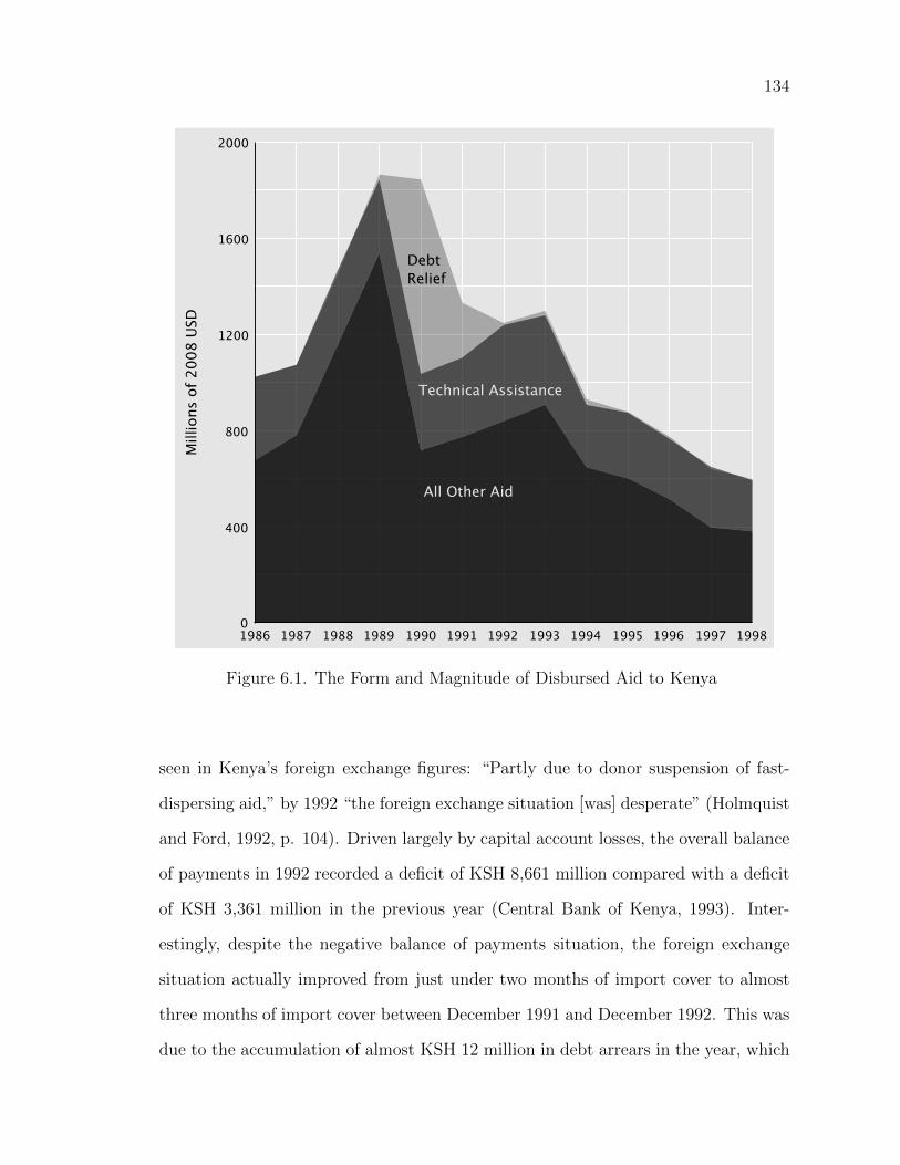
134

19981986 1987 1988 1989 1990 1991 1992 1993 1994 1995 1996 1997

2000

0

400

800

1200

1600

Mill

ions

of 2

008

USD

DebtRelief

Technical Assistance

All Other Aid

Figure 6.1. The Form and Magnitude of Disbursed Aid to Kenya

seen in Kenya’s foreign exchange figures: “Partly due to donor suspension of fast-

dispersing aid,” by 1992 “the foreign exchange situation [was] desperate” (Holmquist

and Ford, 1992, p. 104). Driven largely by capital account losses, the overall balance

of payments in 1992 recorded a deficit of KSH 8,661 million compared with a deficit

of KSH 3,361 million in the previous year (Central Bank of Kenya, 1993). Inter-

estingly, despite the negative balance of payments situation, the foreign exchange

situation actually improved from just under two months of import cover to almost

three months of import cover between December 1991 and December 1992. This was

due to the accumulation of almost KSH 12 million in debt arrears in the year, which

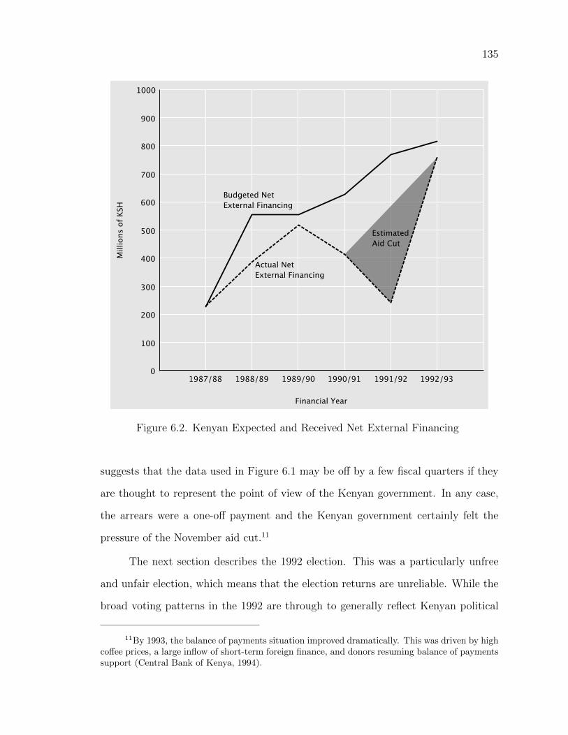
135

1987/88 1988/89 1989/90 1990/91 1991/92 1992/93

1000

0

100

200

300

400

500

600

700

800

900

Financial Year

Mill

ions

of

KSH

Budgeted NetExternal Financing

EstimatedAid Cut

Actual NetExternal Financing

Figure 6.2. Kenyan Expected and Received Net External Financing

suggests that the data used in Figure 6.1 may be o↵ by a few fiscal quarters if they

are thought to represent the point of view of the Kenyan government. In any case,

the arrears were a one-o↵ payment and the Kenyan government certainly felt the

pressure of the November aid cut.11

The next section describes the 1992 election. This was a particularly unfree

and unfair election, which means that the election returns are unreliable. While the

broad voting patterns in the 1992 are through to generally reflect Kenyan political

11By 1993, the balance of payments situation improved dramatically. This was driven by highco↵ee prices, a large inflow of short-term foreign finance, and donors resuming balance of paymentssupport (Central Bank of Kenya, 1994).

136

opinion, the subnational results were almost certainly tainted by voter intimidation

(or worse), ballot box stu�ng, or outright fabrication.

6.1.3 The 1992 Election Results

Before discussing how KANU responded to the aid reduction, it is worth ex-

amining the 1992 election results. In the previous two Chapters, my goal was to

trace out connections between donor finance and election outcomes, showing how

increases or decreases in aid influence the incumbent’s prospects at the polls. The

quality of Kenya’s election—“C-minus” (Barkan, 1993, p. 92)—prevents me from re-

lying heavily on the election results as a reasonable proxy for the will of the people,

so this Chapter takes another strategy.

Due to splits in the opposition and his genuine popularity in parts of Kenya,

Moi would very likely have won the 1992 election if it was completely free and fair

(Throup and Hornsby, 1998, p. 516). In this sense, the outcome of the Presidential

election at the national level approximated the will of the Kenyan people. However,

the election was far from fair,12 and di↵erent areas of the country produced biased

results for di↵erent reasons. This uneven bias in voting prevents sub-national vote

totals from being used as an approximation of the ‘will of the people,’ and so prevents

sub-national comparisons from being valid.

These problems are best illustrated with an example. Baringo is a district in

the Rift Valley in North West Kenya. Moi was very popular in Baringo—he was

born there—and in 1992 he won 95% of Baringo’s vote. Unfortunately, I cannot use

the election results as a reasonable proxy for the will of the people for four reasons.

First, there was a great deal of violence in Rift Valley before the election. The region

12In October, 1992, Moi declared “Tatyari tumeshinda; sasa ni kumaliza tuu. Tunafagia hao

ili wajue chama cha Kanu sio chama cha ukabila (we have already won; we are only putting thefinishing touches and we shall trounce the opposition so that they know that we are not a tribalparty)” (Atemi and Arunda, 1992).

137

experienced state-sponsored ethnic cleansing, in which approximately 1,500 people

were killed and up to 300,000 people were displaced before the election (Africa Watch,

1993, p. 3). Parts of Rift Valley also became ‘no go zones’ for the opposition and they

were “ruthlessly excluded throughout the campaign” (Throup and Hornsby, 1998, p.

464). Commonwealth observers noted “widespread tribal disturbances, threats, and

harassment of party supporters, in particular supporters of the opposition parties”

(Commonwealth Secretariat, 1992, p. x). These problems obviously prevented the

population from expressing their true preferences on election day. Second, in Baringo

many voters were o�cially labeled as illiterate before the election. This meant that

their ballot was filled in by the Presiding O�cer at the polling station, making their

ballot public instead of private (Throup and Hornsby, 1998, p. 428). This also

clearly prevented voters from expressing their true preferences. Third, international

electoral observers feared for their safety in Baringo and none were present on election

day (Throup and Hornsby, 1998, p. 433). Fourth, central Rift Valley, where Baringo

is situated, had 33% higher turnout in 1992 than in 1983. This was the largest gain

in turnout of any region, and makes ballot box stu�ng seem very likely (Throup

and Hornsby, 1998, p. 445). In sum, the election results in three of Baringo’s four

constituencies “were almost certainly fraudulent” (Throup and Hornsby, 1998, p.

465).

The fraudulent, or at least heavily compromised, nature of the electoral data

is a shame, because Baringo was also heavily favoured by the Kenyan state. As

section 6.3.1 will show, Moi clearly favoured his core areas of support when allocat-

ing developmental resources, including aid. In the 1991/92 developmental budget,

Baringo was allocated 5.8 million KSH for minor road construction. This amounts to

15% of all spending (aid and Government of Kenya) on minor roads. Significantly,

donors did not contribute to any construction in Baringo, and Baringo—only one

138

district out of 40 districts in Kenya—absorbed nearly one out of every three shillings

of all locally-raised resources for minor road construction.13 This kind of allocation

around donor funding strongly suggests that aid was fungible and that Moi was able

to spend more on Baringo because donors were building roads elsewhere.14 This

example starkly demonstrates how Moi favoured his base. However, it does not show

that the base voted more for him because of his spending. Ideally, I would compare

a district with high state allocations like Baringo against districts that seem simi-

lar, but received less state support. The problem with this approach is that Moi’s

vote count in Baringo was influenced by many factors that I cannot observe, such as

cheating and violence, and these factors were not even across all districts. It would

be irresponsible to assume that other districts experienced similar problems to sim-

ilar degrees, so I cannot answer the questions of if and how state finance directly

influenced voters in 1992.

Instead, as was noted above, this chapter focuses on Moi’s response to the

aid cut and demonstrates that Moi’s lack of constraints enabled him to take actions

which blunted the political damage that typically occurs when aid quickly declines.

The remainder of the Chapter shows that Moi was able to protect his core areas of

support from the aid cut, that and that he was able to manipulate the economy so

that the e↵ects of the cut were felt after the election and fell disproportionately on

opposition supporters. While the aid reduction put financial pressure on Moi and

was the proximate cause of Kenya’s return to multiparty democracy, Moi retained

13Spending on major roads was not broken down by district, so this example draws only onminor roads. Rift Valley province, which contains Baringo, received over half of all locally-raisedspending on roads in this year.

14As I will show later, this extreme example of fungibility is exceptional. Usually, donorsseemed willing to follow Moi’s agenda. For example, while foreign donors didn’t build any minorroads in Baringo, almost 60% of all aid for minor roads was spent in the Rift Valley. This is aboutdouble what you would expect if you assume that donors wanted to allocate aid equally acrossKenya on a per capita or per square kilometer basis.

139

ample room to maneuver and he made use of it. Thus, this chapter highlights the

importance of discretion in amplifying the positive e↵ect of aid increases and reducing

the negative e↵ect of aid decreases.

6.2 Data Quality and Empirical Strategy

The underlying model driving this dissertation rests on the idea that aid can

be used to produce resources that voters desire and that these resources can increase

the vote for the incumbent president if they are delivered before an election. In

testing this idea in Ghana and Malawi, I was able to use reliable vote numbers.

If vote numbers reflect the aggregated political opinions of the public in a given

constituency then I can use them to assess if aid resources influenced the expressed

will of voters to re-elect an incumbent. Vote returns are thus a way of measuring

public opinion. In Kenya this approach in not possible. In many cases, Kenya’s 1992

vote returns reflect ballot box stu�ng or coercion. Worse (from an empirical point

of view), these problems were not evenly spread across Kenya. This means that

Kenya’s vote returns, which are my measure of the desire of the public to reelect

a president, have measurement error and that that error is not consistent across

constituencies. Finally, it is highly unlikely that these errors are spread randomly

across Kenya. These ‘errors’ are the result of deliberate political manipulations.

All of this means that Kenya’s vote returns—especially its vote returns below the

regional level—cannot be used reliably as a dependent variable.

The Kenyan case, however, is still valuable. First, there is broad consensus

that the regional returns from 1992 generally reflected the will of the people. This

is generally deduced from the presence of ethnic voting and the clear relationships

between regions and political parties (where Rift Valley supported Moi and KANU,

for example). This allows for some weak evidence suggesting causality. More impor-

140

tantly, the Kenyan case allows for an in-depth exploration of the ways that weakly

constrained presidents can shelter themselves from aid reductions. Chapter 2 sug-

gested that aid cuts will be more damaging to highly constrained presidents than to

weakly constrained ones. This Chapter will use counter-factual reasoning to examine

if this holds in the Kenyan case.15 Moi took three kinds of actions to shelter himself

and his supporters from the aid reduction. The first was directing Kenya’s resources

towards his base and away from areas that supported his opponents. The second way

that Moi sheltered his base from the aid cut was through macroeconomic manipula-

tion. Finally, the Kenyan regime undertook a series of violent and fraudulent actions

before the election in an attempt to further influence the vote. The remainder of the

Chapter will analyze these strategies in detail and examine the degree of discretion

required to use them.

6.3 Moi’s Survival Strategies

Section 6.3.1 will examine how the Moi government’s fiscal policies responded

to the aid cut at a subnational level. Section 6.3.2 will examine the government’s

macroeconomic responses. The aid cut may have pushed Moi to hold elections, but

he was clearly able to shelter himself and his supporters from the worst e↵ects of the

cut. Section 6.3.3 will examine the other, mostly illegal, actions that the Kenyan

regime undertook to ensure that Moi won the election. Each section will ask if these

activities could have been undertaken, or could have even been imaginable, if the

Kenyan government (executive) was more constrained.

15For more information on the value of counter-factual reasoning, see Fearon (1991) andLebow (2000).

141

6.3.1 The Geography of Development Spending

This section examines how the Kenyan government re-allocated developmen-

tal resources after aid was reduced in 1991–1993. Generally, Moi and Kenyatta’s

development policies favoured the ethnic groups and regions that supported them

(Barkan and Chege, 1989; Kivuva, 2011), but it is unknown if or how aid (which had

at least nominal donor oversight) was influenced.16 While Moi “explicitly threatened

districts that vote for opposition parliamentarians with loss of o�cial development as-

sistance”(e.g. Harbeson, 1999, p. 51), his ability to actually influence the allocation

of foreign resources according to his own political logic is unknown. If donors have

strong preferences for equality (or simply strong preferences against aiding Moi) and

if they remained informed about aid allocations, then one would expect the Kenyan

government to benefit from aid mainly through fungibility. This would mean that

the government would see where aid was going to be spent and then target their

own resources around the aid allocations to create a politically optimal distribution

of resources. However, it is also possible that donors either did not care where aid

was spent or did not have the ability to police Moi’s spending.

In order to examine the geographical variation of developmental spending, I

examined the developmental budgets of Kenya from 1989 to 1994. I specifically ex-

amine developmental spending on roads and health, as these categories of spending

are reported at a district level and report the source of finance (the government or

the specific donor). This lets me examine variation in spending across both sub-

national units and the source of the funds. The results are first presented according

to Barkan and Chege’s (1989) categorization of regions in Kenya into ‘Moi base’

16Aid to Kenya was disbursed as either grants or leans which which were recorded as revenue,or appropriations-in-aid (A-in-A). Disbursing in A-in-A is more popular with donors because it givesthem more control over the funds. All of the disbursements that I will examine were A-in-A, as aidthat was reported as revenue is impossible to trace. For more information on the details of Kenya’sbudgeting and foreign assistance, see Njeru (2004).

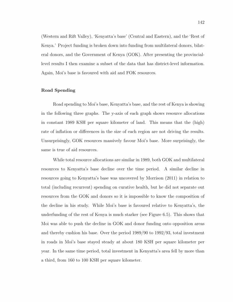
142

(Western and Rift Valley), ‘Kenyatta’s base’ (Central and Eastern), and the ‘Rest of

Kenya.’ Project funding is broken down into funding from multilateral donors, bilat-

eral donors, and the Government of Kenya (GOK). After presenting the provincial-

level results I then examine a subset of the data that has district-level information.

Again, Moi’s base is favoured with aid and FOK resources.

Road Spending

Road spending to Moi’s base, Kenyatta’s base, and the rest of Kenya is showing

in the following three graphs. The y-axis of each graph shows resource allocations

in constant 1989 KSH per square kilometer of land. This means that the (high)

rate of inflation or di↵erences in the size of each region are not driving the results.

Unsurprisingly, GOK resources massively favour Moi’s base. More surprisingly, the

same is true of aid resources.

While total resource allocations are similar in 1989, both GOK and multilateral

resources to Kenyatta’s base decline over the time period. A similar decline in

resources going to Kenyatta’s base was uncovered by Morrison (2011) in relation to

total (including recurrent) spending on curative health, but he did not separate out

resources from the GOK and donors so it is impossible to know the composition of

the decline in his study. While Moi’s base is favoured relative to Kenyatta’s, the

underfunding of the rest of Kenya is much starker (see Figure 6.5). This shows that

Moi was able to push the decline in GOK and donor funding onto opposition areas

and thereby cushion his base. Over the period 1989/90 to 1992/93, total investment

in roads in Moi’s base stayed steady at about 180 KSH per square kilometer per

year. In the same time period, total investment in Kenyatta’s area fell by more than

a third, from 160 to 100 KSH per square kilometer.

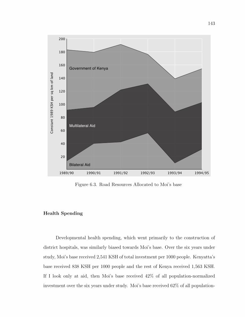
143

1994/951989/90 1990/91 1991/92 1992/93 1993/94

200

20

40

60

80

100

120

140

160

180C

onst

ant

1989

KSH

per

sq

km o

f la

nd

Government of Kenya

Bilateral Aid

Multilateral Aid

Figure 6.3. Road Resources Allocated to Moi’s base

Health Spending

Developmental health spending, which went primarily to the construction of

district hospitals, was similarly biased towards Moi’s base. Over the six years under

study, Moi’s base received 2,541 KSH of total investment per 1000 people. Kenyatta’s

base received 838 KSH per 1000 people and the rest of Kenya received 1,563 KSH.

If I look only at aid, then Moi’s base received 42% of all population-normalized

investment over the six years under study. Moi’s base received 62% of all population-

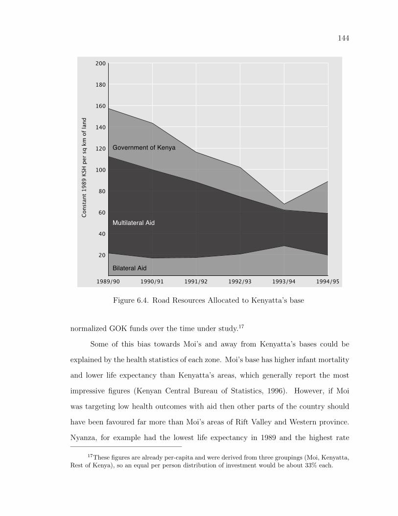
144

1994/951989/90 1990/91 1991/92 1992/93 1993/94

200

20

40

60

80

100

120

140

160

180C

onst

ant

1989

KSH

per

sq

km o

f la

nd

Government of Kenya

Bilateral Aid

Multilateral Aid

Figure 6.4. Road Resources Allocated to Kenyatta’s base

normalized GOK funds over the time under study.17

Some of this bias towards Moi’s and away from Kenyatta’s bases could be

explained by the health statistics of each zone. Moi’s base has higher infant mortality

and lower life expectancy than Kenyatta’s areas, which generally report the most

impressive figures (Kenyan Central Bureau of Statistics, 1996). However, if Moi

was targeting low health outcomes with aid then other parts of the country should

have been favoured far more than Moi’s areas of Rift Valley and Western province.

Nyanza, for example had the lowest life expectancy in 1989 and the highest rate

17These figures are already per-capita and were derived from three groupings (Moi, Kenyatta,Rest of Kenya), so an equal per person distribution of investment would be about 33% each.

145

1994/951989/90 1990/91 1991/92 1992/93 1993/94

200

20

40

60

80

100

120

140

160

180C

onst

ant

1989

KSH

per

sq

km o

f la

nd

Government of Kenya

Bilateral Aid

Multilateral Aid

Figure 6.5. Road Resources Allocated to the Remainder of Kenya

of infant mortality.18 Despite this, Nyanza received very low resource allocations,

either in raw figures or per capita or per square kilometre. A government that was

targeting low life expectancy or high infant mortality would indeed allocate away

from Kenyatta’s base, but it would not direct many additional resources to Moi’s

areas. The preferential treatment shown to Moi’s base is far too large to be explained

by low health outcomes, and if Moi was targeting low health outcomes then other

parts of the country should have been a much higher priority. The best explanation

18Life expectancy in Nyanza was 49.5 years in the period 1979-1989. This was ten years lessthan Rift Valley and fifteen years less than Eastern province (Kenyan Central Bureau of Statistics,1996).

146

is that domestic political calculations were driving most of the allocations to Moi’s

base.

District-Level Health Spending

While the provincial-level analyses above are standard in the literature (Barkan

and Chege, 1989; Morrison, 2011), they operate at a very high level of aggregation.

In particular, certain parts of Rift Valley were not part of Moi’s ethnic base. This

section uses a subset of the main dataset that contains information on district-level

allocations to show that, at a district level, donor-funded aid and GOK resources

also favored Moi’s ethnic areas and the ethnic areas where he attempted to curry

favor. About half of all spending (GOK and donor) in the previously used roads and

health dataset lists the district to which the funds were allocated.19 The district-

level resource allocation figures are quite lumpy year-to-year so they were pooled

over time. This means that we lose the time dimension of the provincial analysis,

but in its place we gain much more detailed subnational information. The number of

districts changes over the time period, and where possible split districts were merged

back to the 1989 districts for the analysis.20 The 1989 census recorded district-level

information on ethnicity. This information was used to code the largest ethnic group

for each district. I also use data on population, area, and infant mortality from the

1989 census. Population, area, and all resources figure are in thousands.21 In this

time period, Moi’s ethnic coalition was made up of the Kalenjin and Masai and a

19The remaining half of the spending lists only the province.

20The splits usually occurred later in the time period and generally merging split districtswas straightforward. Thika district was merged back into Kiambu, Nyamira was merged intoKisii, Homa Bay was merged into South Nyanza, Elgeyo was counted as funding towards ElgeyoMarakwet, and Vihigia was part of Kakamega. I was unable to find a match for a small amountof resources to a small number of districts. The unmatched resources were 0.003% of the totalresources in the district-level subset of the data.

21Resources figures are in thousands of constant 1989 Kenyan shillings. Infant mortality isper 1000 live births.

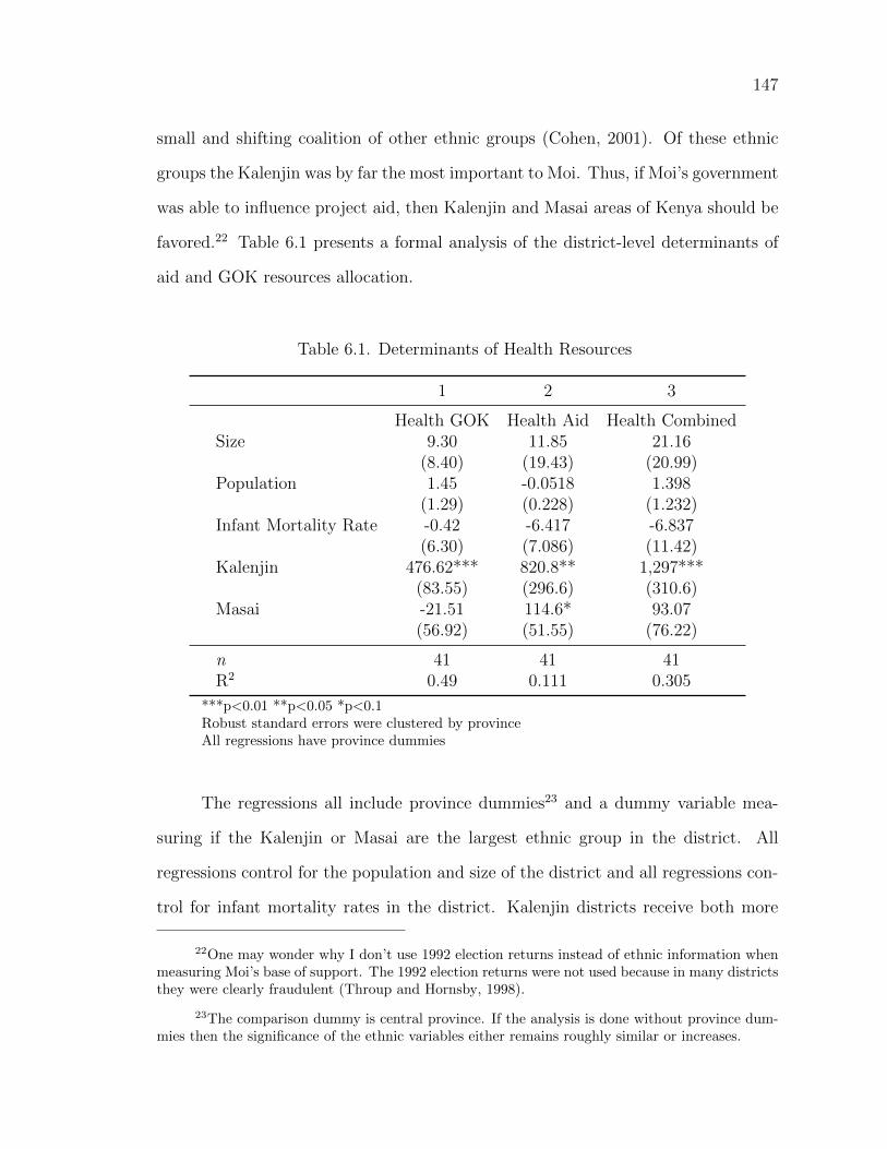
147

small and shifting coalition of other ethnic groups (Cohen, 2001). Of these ethnic

groups the Kalenjin was by far the most important to Moi. Thus, if Moi’s government

was able to influence project aid, then Kalenjin and Masai areas of Kenya should be

favored.22 Table 6.1 presents a formal analysis of the district-level determinants of

aid and GOK resources allocation.

Table 6.1. Determinants of Health Resources

1 2 3

Health GOK Health Aid Health CombinedSize 9.30 11.85 21.16

(8.40) (19.43) (20.99)Population 1.45 -0.0518 1.398

(1.29) (0.228) (1.232)Infant Mortality Rate -0.42 -6.417 -6.837

(6.30) (7.086) (11.42)Kalenjin 476.62*** 820.8** 1,297***

(83.55) (296.6) (310.6)Masai -21.51 114.6* 93.07

(56.92) (51.55) (76.22)

n 41 41 41R2 0.49 0.111 0.305

***p<0.01 **p<0.05 *p<0.1Robust standard errors were clustered by provinceAll regressions have province dummies

The regressions all include province dummies23 and a dummy variable mea-

suring if the Kalenjin or Masai are the largest ethnic group in the district. All

regressions control for the population and size of the district and all regressions con-

trol for infant mortality rates in the district. Kalenjin districts receive both more

22One may wonder why I don’t use 1992 election returns instead of ethnic information whenmeasuring Moi’s base of support. The 1992 election returns were not used because in many districtsthey were clearly fraudulent (Throup and Hornsby, 1998).

23The comparison dummy is central province. If the analysis is done without province dum-mies then the significance of the ethnic variables either remains roughly similar or increases.

148

GOK resources and more aid. Masai districts also receive more aid, but not more

GOK resources. The Western province dummy is also significant at 0=0.1 and posi-

tive. This suggests that the province (predominantly Luhya) was also favoured with

GOK resources. Sadly, infant mortality (from the period 1979-1989) is weakly and

negatively related to resources for district hospitals. Aid and GOK funding for hos-

pitals was not been allocated according to need. Instead, it was strongly influenced

by ethnic politics.

The district-level and province-level evidence supports the claim that aid projects

and less-surprisingly, GOK spending, were being influenced by Moi’s ethno-political

calculations. Moi’s provinces received far more aid that one would expect based on

need, area, or population. When aid resources declined over time, Moi’s provinces

were largely saved from resource cuts, which were instead pushed on to Kenyatta’s

provinces. This time trend suggests that donors were not moving away from Moi’s

areas as time went on. The idea that Moi’s areas were favored is further support by

the district-level subset of the provincial data. Districts where the Kalenjin or Masai

were the largest ethnic group received more aid and GOK resources than districts

with other ethnic groups, and this finding generally holds within provinces as well as

across Kenya. At both the provincial and the district level, and across time, project

aid disproportionately favored Moi’s ethnic areas. This concentration and shift in

resources meant that Moi’s areas benefited most from foreign aid and were hurt least

by declines in aid.

How important was discretion?

It is not clear how Moi was able to allocate such a large fraction of foreign

resources to his base, but regardless of the precise mechanisms the final outcome

149

is the same.24 The parts of Kenya that most supported Moi saw their resource

allocations barely fall during the aid cut. The opposition areas fared much worse.

Domestic discretion was fairly important here because this could not have happened

unless Moi and his coalition had control over the national budget. This level of

executive discretion over the budget, however, was not unique to Kenya. It is likely

that many more countries could have engineered this kind of skewing. While the

comparison is not direct, in Chapter 4 we saw Ghana’s NDC arrange a similarly

political transfer of donor resources. This kind of activity thus would likely have

been possible in most other African electoral democracies with strong presidents.

6.3.2 Macroeconomic Survival Strategies

Moi’s survival strategies went beyond fiscal policies and his successful attempts

to shift the burden of declining resources onto segments of the population that sup-

ported his opponents. Macroeconomic manipulations were also an important part of

Moi’s ability to retain political control in the face of declining international support.

While the surprise aid cut meant that the government clearly expected more revenue

from abroad, “technocrats in the Central Bank and the Ministry of Finance adapted

[...] regardless of the cost to the country’s economic health” (Throup and Hornsby,

1998, p. 583).

Deficit Finance and Inflation

The Kenyan government’s macroeconomic response to the reduction in foreign

financing was twofold. First, they did reduce spending somewhat. Second, they

shifted from foreign deficit finance to domestic deficit finance. This shift is shown

in Figure 6.6. High domestic borrowing predictably led to an increase in inflation

24I explain this outcome using bargaining model where donors lack complete information onthe allocations of other donors. The paper is currently R&R at SCID.

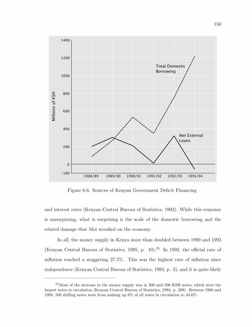
150

1400

-100

0

200

400

600

800

1000

1200M

illio

ns o

f KS

H

1990/91 1991/92 1992/931989/90 1993/94 1988/89

Total DomesticBorrowing

Net ExternalLoans

Figure 6.6. Sources of Kenyan Government Deficit Financing

and interest rates (Kenyan Central Bureau of Statistics, 1992). While this response

is unsurprising, what is surprising is the scale of the domestic borrowing and the

related damage that Moi wreaked on the economy.

In all, the money supply in Kenya more than doubled between 1990 and 1993

(Kenyan Central Bureau of Statistics, 1995, p. 10).25 In 1992, the o�cial rate of

inflation reached a staggering 27.5%. This was the highest rate of inflation since

independence (Kenyan Central Bureau of Statistics, 1993, p. 3), and it is quite likely

25Most of the increase in the money supply was in 200 and 500 KSH notes, which were thelargest notes in circulation (Kenyan Central Bureau of Statistics, 1994, p. 209). Between 1988 and1993, 500 shilling notes went from making up 6% of all notes in circulation to 43.6%.

151

an underestimate (Holmquist and Ford, 1992, p. 104). An external estimate for

the inflation rate in 1993 was 55% (O’Brien and Ryan, 2001, p. 491). During only

the last quarter of 1992, right before the election, the money supply was estimated

to have increased 40% (Barkan, 1993, p. 94), prompting FORD-Kenya candidate

Oginga Odinga to make inflation central to pre-election his Christmas message to

Kenyan voters (Daily Nation, 1992). With inflation this high, the nominal wage

increases that occurred after 1991 were outstripped and real earnings declined by

8.3% in 1991 and 12% in 1992 (Kenyan Central Bureau of Statistics, 1993, p. 51).

Over the period, the government-reported annual GDP growth rate fell constantly

from 5.2% in 1988 to 0.2% in 1993 (Kenyan Central Bureau of Statistics, 1992, 1995).

Finally, by 1993 the real rate of interest was -10.8% (World Bank, 1996, p. 39).

While some of the costs of inflation would have hurt all Kenyans, those in the

formal economy would have been worst hit. Inflation most hurts those with savings

in the local currency and those on salaries. While there is no evidence that this

was part of Moi’s calculation, the segments of the population that owned businesses

or were on fixed government salaries tended to be opposition supporters. Moi did

not plan on winning these more urban areas, and in the general election KANU

was beaten in 15 of 20 of Kenya’s principal town and municipal councils, including

Nairobi (Barkan, 1993). When donors reduced support to Kenya, Moi’s government

shifted to borrowing from the domestic economy rather than drastically reducing

spending. This let the government continue with its largesse before the election.

While this hurt everyone, the costs were more acutely felt in urban, opposition areas

where people relied more heavily on the formal economy.

How important was discretion?

These kinds of monetary manipulations directly contradicted very basic guide-

lines for monetary policy (e.g. don’t increase the money supply by 40% in one

152

quarter). They also led to a “financial crisis” (World Bank, 1996, p. 5) which only

truly arrived after the elections. The actions of the Moi regime showed that they

had a great deal of discretion over monetary policy. Had Moi been more constrained

in his access to the printing press or had his government been more restrained in its

access to finance from the Central Bank, then the Kenyan government would have

had to more radically reduce spending in the face of declining overseas transfers.

While it is impossible to know precisely what would have happened if the Kenyan

government would have been forced to cut back radically on spending, it seems rea-

sonable to conclude that Moi would have been less popular across Kenya, especially

in the areas that benefitted from his largesse, and he probably would have done worse

in the 1992 election. Given the role of money in holding Kenyan ruling coalitions

together, lower resource flows before a critical moment like an election would surely

have harmed Moi and KANU. Moi’s large degree of discretion over monetary policy,

broadly defined, thus helped him blunt the e↵ect of the aid decline.

6.3.3 Theft, Fraud, and Violence

While the previous sections have discussed how Moi was able to re-allocate

state spending geographically to shelter his base and how he was able to manipu-

late the economy, those actions did not mark the limits of his manipulations. This

section overviews the election-related theft and fraud that occurred under Moi. One

high ranking bureaucrat called corruption, “[Kenya’s] biggest economic problem”

(Holmquist and Ford, 1992, p. 104). This section confirms the scope of the prob-

lem under Moi and links this corruption to KANU’s campaign finance requirements

in 1992. The money in this section was wholly illicit and thus not subject to any

oversight or constraints. This makes it basically impossible to trace and, because

of this, makes it Moi’s most politically valuable resource. While I therefore cannot

show direct connections, the consensus position of most observers is that all of the

153

following scandals had strong links to KANU’s 1992 campaign.

Corruption at the Central Bank

As we saw in section 6.3.2, inflation in Kenya was running at all time highs in

the 1990s. Part of this was certainly due to deficit finance and Moi’s macroeconomic

planning. However, part of the increase in inflation was also the result of corruption

connected to campaign finance. Joel Barkan (1993, p. 94) has argued that the 40%

increase in money supply in the quarter before the election was due to “the flow

of money from the Central Bank of Kenya to the president and KANU nominees.”

Waindi (2010, p. 46) noted KANU funded its campaign “by giving a few banks

unlimited access to overdraft facilities at the Central Bank of Kenya, something

akin to printing paper money.” This problem was confirmed by the World Bank,

whose “IMF/IDA review missions in Autumn 1992 and Spring 1993 found evidence

of significant violation [sic] of monetary targets, due to abuse of the preshipment

export financing scheme26 and access of certain commercial banks to Central Bank

of Kenya (CBK) overdraft and rediscount facilities” (World Bank, 1996, p. 2). The

e↵ect of domestic deficit financing, printing money, and other questionable monetary

dealings on inflation was nicely summarized by the Kenyan Minister for Transport,

Mr. Otieno, on 24th of March, 1993:

“Mr. Speaker, Sir, it should be understood that the Kenyan budget has beenfinanced by foreign assistance for many years since Independence and that whenthis stopped for 16 months one source of excess money supply was the bud-get deficit. Another source of excess money supply was the money which wepoliticians must have kept in the mattresses and we released it all during thecampaign. [...] Another source of excess money supply must be money whichwe politicians kept abroad and brought it in for the purposes of the campaignthrough the Forex-C market and changed it into Kenya shillings. A possibleother source of excess money supply were donations which some of us must have

26The preshipment export financing scheme problems are most likely linked to the GoldenbergScam, which is discussed below.

154

generously received to finance their political activities” (Government of Kenya,1993, p. 56).

The Kenyan government’s domestic borrowing produced an increase in money

supply. This probably would not have happened if Moi had been more constrained.

However, those manipulations pale in comparison to the finding that KANU had

“unlimited access to overdraft facilities at the Central Bank” (Waindi, 2010, p. 46).

Operations Moi Wins, a KANU support group that at times “was blatantly paying

voters” was responded to a question about its funding by saying that the group

would spend “an amount of money you have never seen before” (Ondieki, 1992). It

is estimated that KANU spent about 60 million US dollars on vote buying (Foeken

and Dietz, 2000, p. 135).27 While this is shocking, this is only one of the brazenly

corrupt actions taken by KANU in the run up to the 1992 election.

Stealing from the Social Security Fund

Another source of campaign finance for Moi’s campaign came from outright

theft from the National Social Security Fund (NSSF). When the story was originally

broken in late 1992 by Kenya’s The Daily Nation, Youth for Kanu ’92 protested out-

side the paper’s headquarters (Niko, 1992). Despite numerous claims to the contrary,

the links between KANU and the NSSF are quite clear:

“It was reported that in 1992, the National Social Security Fund ‘loaned’ Ksh.1.2 billion to a private company owned by a KANU o�cial and a civil servant.In the same year, the said institution made further disbursements of Ksh. 0.54billion and 0.3 billion to the ‘Youth for KANU 92’ and the private company,respectively. These monies were said to be for campaigning for President Moi’sre-election and to bribe his political opponents” (Waindi, 2010, p. 44–45).

The quote above did a good job of summarizing the situation as of 2010, but

thanks to continuing interest in this scam, a few more details of this story are now

27The authors are unclear on the source of the figure, but a number of KANU support groups,especially YK’92 are widely known to have spent large sums of money attempting to influence votersbefore the 1992 election.

155

available. These details help to show how the KANU government was able to transfer

resources our of the NSSF to its own politicians. For example, in September of 1992

the NSSF “bought two plots from Sololo Outlets, a firm owned by Mr. Cyrus Jirongo

who was then the chairman of the defunct KANU campaign lobby group, Youth for

KANU 92” (Njau, 1998). Mr. Jirongo was also a KANU MP for Lugari, a district

in Western Province (Rubadiri, 2012). The deal was simply a way to move funds

from the NSSF to KANU, and the authorization to make the purchase ran back to

high-level KANU politicians. The NSSF’s acting Managing Trustee, Tom Odongo,

claimed that the directive to buy the property “did not come directly from Sololo to

NSSF. It was a directive that we received from the then Permanent Secretary [of the]

Ministry of Finance” (Rubadiri, 2012). The Permanent Secretary, Wilfred Koinange,

was said to have acted with the full knowledge of the Vice President George Saitoti,

who was also the Minister of Finance at the time (Rubadiri, 2012). Mr. Koinange

wrote two letters to the NSSF about these land deals (Oruko, 2012). The first, dated

June 23, 1992, pressed the NSSF to invest in the properties. In the second letter,

in late September, “Koinange [ordered the] NSSF to deposit KSH300 million to the

accounts of Sololo to commence the works.” The project was later canceled, after

about three-quarters of the work was done and the resolution of the matter is still

ongoing (Oruko, 2012). After summoning the main parties before parliament and

questioning them in April of 2012, the MPs were reported to have considered the

deal “suspicious” and “meant to allegedly raise money for the 1992 general election”

(Oruko, 2012). While there are still many murky details, there is a broad consensus

that “in the 1992 General Election, the NSSF was raided by Kanu operatives for

money to finance the poll and enrich themselves” (Opala, 2003).28

28This was simply a selection from a batch of scams surrounding Kenyan government bodiesand various KANU groups. YK ’92, for example, was spending so much money that it was “clearthat only the government could be providing the funds.” (Throup and Hornsby, 1998, p. 355).This was then norm, and “most KANU candidates” received money from either President Moi,

156

The Goldenberg Scam

The Goldenberg scam involved the purported export of diamonds (of which

Kenya had basically none) and then the filing of fabricated export compensation

claims with the Central Bank of Kenya. This scam was already alluded to in the

World Bank quote mentioned in section 6.3.3. In more detail, it involved a compli-

cated “series of business deals or alleged business deals revolving [sic] round various

economic schemes to wit, Export Compensation, Pre-shipment Finance, Retention

Accounts, Forex Cs, Spot and Forward Contracts, cheque kiting and outright theft”

(Bosire, 2005, p. 25).

The Goldenberg scam may have links to President Moi’s electoral campaign.

The problem here is that many of the financial details of the Goldenberg scam remain

hidden. The best evidence for a link between Goldenberg and KANU comes from

Kamlesh Pattni, the main actor behind the Goldenberg A↵air. He claimed to have

spent a great deal on Moi’s campaign, but his testimony on this matter was wildly

exaggerated and seemed to suggest that he was either trying to pull down important

figures with him or simply trying to seem more important. The relevant parts of the

report are well summarized by Waindi (2010, p. 46–47):29

“The Bosire Commission received evidence that Kamlesh Pattni, a key protag-onist in the Goldenberg Scandal, had agreed with President Moi that Pattniwould directly and through his companies finance KANU in the 1992 elections.The witness estimated that he spent more than Ksh. 4 billion (USD 57,000,000)in election related expenses. The Bosire Commission found in this regard, thatalthough it was not possible to ascertain the amount, nature and extent of suchpolitical financing, Pattni’s statement that he gave KANU support was on thewhole plausible.”

The figure of 4 billion KSH, even if it was spread over two years,30 is unbeliev-

KANU headquarters or other KANU organizations (Throup and Hornsby, 1998, p. 357).

29The original source is Bosire (2005, p. 181–196).

30The election was announced in late 1991 and held in late 1992. Thus, Pattni could perhaps

157

able. To put this figure in context, the Kenyan government’s entire budget was well

under 4 billion KSH in 1991/92, and in 1991 the money supply of Kenya was 3.7

billion KSH (Kenyan Central Bureau of Statistics, 1995, p. 79 & 10). My conclusion

is therefore in line with the Goldenberg Report. While 4 billion KSH is likely an

exaggeration, the idea that Pattni gave support to Moi is plausible. It seems unlikely

that a scam of this magnitude could have existed without the blessing, if not active

support, of high-level politicians.31

Election-Related Violence

Finally, the Moi regime benefited from ethnic violence in the Rift Valley.32 This

violence began on October 29, 1991 and within a few years “would leave thousands

dead, almost half a million displaced and hundreds of thousands e↵ectively disen-

franchised” (Klopp, 2001, p. 133). While the violence was sparked by land disputes,

it had taken on an ethnic component within months. The initial violence may have

had little to do with the election, though unsurprisingly “the newly legalized political

opposition was quick to blame the ethnic clashes on the KANU government’s fear

of losing the election” (Africa Watch, 1993, p. 28). This claim is echoed by Klopp,

whose thesis puts forward the argument that:

“this unprecedented level of violence, and the related withdrawal of state protec-tion for private rights to land, were fundamentally linked to genuine challengesto patrimonial control. Key members of a besieged KANU regime strategizedto counter political change by playing on grievances generated by a history ofexclusionary and irregular land allocations. Through revival of a majimbo orethno-regional discourse ascribing rights to land based on ethnic identity, which,in turn, was linked to support for the KANU government, key patronage bosses

have spread the ‘election related expenses’ out over a little more than one year at maximum.

31My interpretation of the evidence is conservative. Others are far more willing to claim thatMoi, Vice-President George Saitoti, and KANU were actively involved in the Goldenberg A↵airand that it was linked to the 1992 election (Mutua, 2008; Barkan, 1999; Dowden, 2011).

32This section draws heavily on a report by Africa Watch (1993) and a dissertation by Klopp(2001).

158

attempted to divert often profound grievances around land into an electorallybeneficial politics” (Klopp, 2001, p. 133–134).

Violence was particularly useful to a KANU regime with shrinking resources

because it was essentially free over the short-term. Instead of o↵ering voters a share of

declining patronage resources, KANU was able to encourage violence that disenfran-

chised likely anti-KANU voters and redistributed their land to KANU supporters.33

This explanation fits the pattern of violence well, with its clear ramp up before the

election. By February of 1992, after elections were announced, the conflict had grown

in intensity and become more overtly political. In March 1992, for example, “Kalen-

jin Assistant Minister Kipkalia Kones, declared that Kericho District was a KANU

zone and added that anyone who supported the political opposition would ‘live to

regret it’ ” (Africa Watch, 1993, p.29). The final result was that:

“By the time the election was held on December 29, 1992, thousands of Kenyanswere unable to cast their ballot as a result of the displacement and destructioncaused by the ethnic clashes. Many eligible voters had lost property titles oridentification that would have enabled them to register to vote. Others wereunable to return to their home areas to vote” (Africa Watch, 1993, p. 35).

This dual strategy of depriving likely opposition supporters of both their land

and their vote was “not only politically useful for patronage bosses but, over the

short term, e↵ective in winning elections and reinforcing local domination” (Klopp,

2001, p. 134). The largest empirical challenge to the view that the violence was part

of a loosely coordinated KANU plan to entrench their control is the fact that the

violence continued well after the election. The continuation of violence after the 1992

election lead Throup and Hornsby (1998, p. 541-42) to claim that the ethnic clashes

33A similar motive was possibly at play when the Kenyan government banned the movementof maize in November of 1992. This happened amid allegations that food aid was being used beforethe election to induce voters (Makokha, 1992; Nation Correspondent, 1992). Throup and Hornsby(1998, p. 358–59) also describe the use of food aid to buy votes and report that it appeared “tohave been an e↵ective tactic in some marginal areas.”

159

were not motivated by the elections, but this is not a majority view. Klopp (2001,

Chapter 4) claims that the violence persisted past the elections because it was useful

for national bargaining as well as electoral gains. Medard (1996) points out that

if you actually look at the players involved in organizing the violence, they include

politicians who were definitely thinking about upcoming elections.34 For Medard,

these elections include the 1992 and the 1997 elections, which helps explain why the

violence didn’t stop after 1992.

How important was discretion?

For each of the activities in this final section, ‘discretion’ barely covers what

the Moi regime was able to do to help Moi secure re-election. The term discretion

implies that someone has a say over the outcome of some decision, and is not bound

by rules. It is typically applied to decisions made when going about one’s job in

an important position, so it applies well to presidents. They have a great deal of

discretion over budgets if they face few formal or informal checks on their ability

to achieve their budgetary preferences. The activities described in this section were

brazenly illegal. The Kenyan regime killed people, stole from social security, and

printed vast sums of money before the 1992 election. This doesn’t reflect discretion

in the typical sense of the word. These are the actions of a regime that views itself

as above the law and was committed to winning an election no matter the cost.

All of these actions would have been nearly unthinkable in a country with a more

constrained president.

34Boone (2011) also broadly supports the argument that land rights were manipulated forpolitical gain and that these manipulations catalyzed violence.

160

6.4 Conclusion

6.4.1 Explaining Moi’s response to the aid cut

Considering how Moi was able to alter subnational development spending,

manipulate the economy, and amass a war chest of campaign finance through brazen

theft, it is surprising that Moi capitulated in the face of the November aid cut. As was

noted before, non-debt relief aid to Kenya was increasing throughout 1990–1993, so

even if the government was getting less than it expected, Kenya as a country was not

experiencing a decline in aid. Further, Moi was clearly capable of running the state

on domestic borrowing, at least for the short-term. Why then did he reintroduce

multiparty politics? One explanation is that Moi and his inner circle “overestimated

the immediate impact of the cessation of balance of payments support,” “panicked,”

and then “cracked”(Throup and Hornsby, 1998, p. 583). This view is reinforced

by a comment from Terry Ryan, who spent time as a Permanent Secretary in the

Ministry of Finance and an Economic Secretary to the Treasury, who wryly noted

that “the thing about foreign exchange is that you can’t create it.” He also made

it clear that the Kenyan Consultative Group Delegation was genuinely surprised by

the donors’ decision to cut balance of payments support.35 It is certainly possible

that Moi simply cracked under pressure. Another explanation is that Moi did not

fear the aid reduction so much as the potential influence of the IMF and World Bank

on Kenya’s credit rating, and Moi saw the aid cut as an ominous sign that required

a clear response in order to avoid a downgrade (Klopp, 2001, p. 118).

A similar explanation is that Moi feared not the immediate e↵ect of the aid

reduction but a further deterioration of donor support over time. This is in fact what

happened, as aid declined precipitously from 1993 to 1999 (see Figure 6.1). Moi may

have interpreted the aid cut a signal that the good times were quickly ending, and

35Interview at the Central Bank in Nairobi on August 29, 2011.

161

that he should begin to open up politics while he still had ample resources and the

ability to control the democratic process. In this argument:

“The willingness to hold multiparty elections was a calculated risk with theregime betting that it was easier to meet the challenge of democracy than run apatronage-based regime without substantial international aid flows”(Holmquistet al., 1994, p. 99).

If this was his calculation, then it was astute. Moi retained enough control over

Kenya’s politics and economics to hold a ‘C-minus’ election without truly having to

fear turnover. Moi also cleverly played to donors’ fear of political breakdown in a

way that allowed him to avoid being penalized for his actions (Brown, 2001). While

aid continued to decline throughout the 1990s, Moi was able to win the 1997 election

with a slightly larger margin. Hopes for electoral turnover were high in 1992, but it

would have to wait another decade.

6.4.2 Kenya in comparative perspective

The Kenyan case tells us a number of things about the mechanisms that link

aid changes in incumbent advantage. With the crudest view of the data, the Kenyan

case does not pose a problem for the theory that aid changes influence incumbent

advantage. Even if the government of Kenya was experiencing aid declines, the

country as a whole saw net usable ODA increases over this time period. If we dig

deeper, then we see that the framework from Chapter 2 become quite useful. In

particular, the Kenyan case shows how donors can try (and also fail) to control aid

and how unconstrained governments can take actions to limit the political fallout

which can arise from a reduction in aid before an election (see Table 2.1). As this

Chapter has shown, Moi was able to use his freedom and power to accomplish four

things:

1. Moi was able to shelter his base from declines in developmental resources.

162

2. Moi was able to ensure that the government could continue to run on short-term

borrowing and other macroeconomic manipulations rather than undergo significant

reductions in government spending.

3. KANU was able to secure a very large amount of campaign finance through illegal

and quasi-legal means.

4. The regime was able to stoke and encourage violence against ethnic groups likely

to vote against Moi in key parts of Kenya.

While all of these actions helped Moi win the election, they were only important

because the opposition remained divided. While the opposition did face “continual

harassment,” it “beat itself by not staying united” (Barkan, 1993, p. 97). Thus, it

is important to remember that while Moi was able to use his unconstrained powers

to blunt the political e↵ects of the aid cut, the main factor behind the opposition’s

loss was not any combination of Moi’s actions but rather the opposition’s inability

to unite. Domestic politics thus doubly shaped the outcome of this election, first by

presenting Moi with a fragmented opposition and then by acting as an intervening

variable that blunted the e↵ect of international systemic forces on local political

outcomes.

Discretion and aid allocations

The Chapter also shows that the mechanisms that might link aid to incumbent

advantage are likely determined more by recipient politics than by donor policies.

While donors were able to push Moi towards holding an election, they could not

stop their aid from flowing disproportionately to Moi’s base. This was the case

even though this foreign aid was not given directly to the budget, but instead was

transferred from the donor to the Ministry or project coordinator on a per project

basis (Njeru, 2004). Donors likely lost control of this aid because while donors

163

still monitored the aid, it flowed through the Kenyan state and often required the

Kenyan state to be actively involved in planning (e.g. adding to road networks). This

funneling of money through the state gave the Kenyan government more control than

donors intended.

In Kenya in 1992, government control of aid meant that Moi had control of

aid because he faced so few domestic constraints on his use of power. By the end of

the 1990s, “the [Kenyan] executive had become too powerful for any institution to

check it” (Kivuva, 2011, p. 6). Many of Moi’s actions would have been unthinkable

in an institutional context with more executive constraints. These lack of constraints

explain both why Moi was able to control the aid that did pass through the Kenyan

government and also why he was able to cope well with the shortfalls in aid that

the Kenyan government experienced. The lack of reliable election data makes it

impossible to precisely measure the e↵ect of foreign aid, and its decline, on Moi’s

election results. However, we can be confident in asserting that Moi would have done

worse had he faced more constraints on his power. Moi’s large degree of discretion

was invaluable in blunting the e↵ect of the aid cut and in winning the 1992 election.

164

CHAPTER 7

CONCLUSION

Foreign aid is a volatile source of finance. Aid volatility harms the economy

and hampers economic planning (e.g. Bulir and Hamann, 2008), but the politics

e↵ects of aid volatility have been largely ignored. This is surprising, because foreign

aid remains an important source of government finance in Africa (see Figure 7.1)

and the volatility of aid is not declining over time (see Figure 1.1).

This dissertation has argued that foreign aid volatility influences election out-

comes in Africa. It examined two mechanisms that could link aid to votes. First, it

is possible that foreign aid provides local public goods to retrospective voters, and

that voters like these goods and so vote more for the president. There is evidence

that this happened in Ghana with aid for electricity (chapter 4) and in Malawi with

teacher training and school construction (chapter 5). Second, foreign aid could be

stolen and channeled to narrow groups of voters. This also happened in Malawi,

when contracts for school construction were ‘won’ by incumbent politicians who

used the money for campaigning and did not build the schools. The dissertation

also examined if recipient discretion could change the magnitude of the influence

of aid changes on election outcomes. It was found that discretion can amplify the

e↵ect of an aid increase and dampen the e↵ect of an aid decrease. The power of

discretion was mostly clearly shown in the case of Kenya (chapter 6), when Moi was

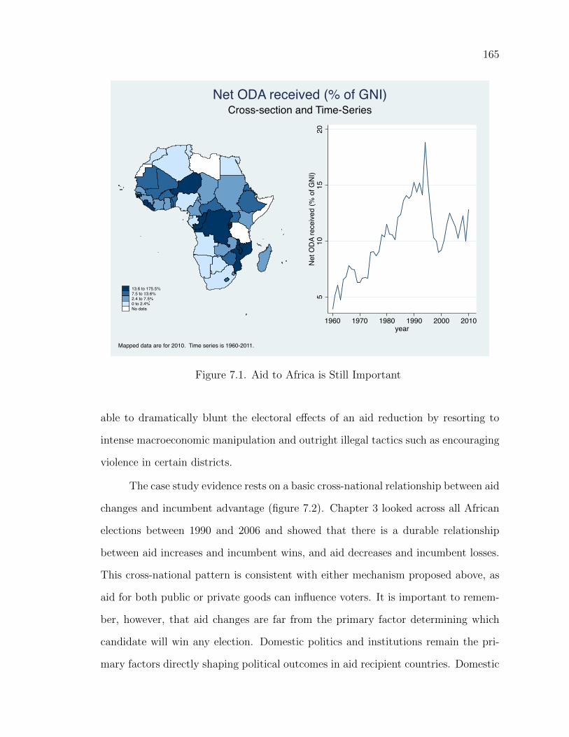
165

13.6 to 175.5%7.5 to 13.6%2.4 to 7.5%0 to 2.4%No data

510

1520

Net O

DA re

ceive

d (%

of G

NI)

1960 1970 1980 1990 2000 2010year

Mapped data are for 2010. Time series is 1960-2011.

Cross-section and Time-SeriesNet ODA received (% of GNI)

Figure 7.1. Aid to Africa is Still Important

able to dramatically blunt the electoral e↵ects of an aid reduction by resorting to

intense macroeconomic manipulation and outright illegal tactics such as encouraging

violence in certain districts.

The case study evidence rests on a basic cross-national relationship between aid

changes and incumbent advantage (figure 7.2). Chapter 3 looked across all African

elections between 1990 and 2006 and showed that there is a durable relationship

between aid increases and incumbent wins, and aid decreases and incumbent losses.

This cross-national pattern is consistent with either mechanism proposed above, as

aid for both public or private goods can influence voters. It is important to remem-

ber, however, that aid changes are far from the primary factor determining which

candidate will win any election. Domestic politics and institutions remain the pri-

mary factors directly shaping political outcomes in aid recipient countries. Domestic

166

institutions also directly a↵ect the magnitude of the influence of aid changes by af-

fecting how politicians can respond to the change. With high discretion, politicians

can closely target aid increases to areas where they will be most politically useful.

There was evidence of this kind of targeting in all cases. Discretion also allows recip-

ients to reduce the e↵ect of a drop in aid. This was most clearly shown in the Kenyan

case (chapter 6), which revealed that when incumbent presidents are unconstrained

they can create the conditions that all but guarantee their re-election. Though aid

changes influence incumbent advantage, aid helps incumbents more and hurts them

less when recipient presidents face fewer domestic constraints on their power and

thus have more options for responding to the aid change.

There is ample evidence linking incumbent advantage in Africa to the ability

of presidents to control state finances (Nugent, 2001; Wantchekon, 2003), and foreign

aid is an important source of government finance in many countries in Africa. Thus,

the while the links between incumbent advantage and aid volatility have never been

analyzed, the arguments fit within well established theoretical frameworks. The

dissertation makes more theoretical contributions in its analysis of the specific ways

that foreign aid influences election outcomes and in its sensitivity to the interactions

between domestic discretion and foreign aid. The specific ways that foreign aid

influence outcomes upsets some strongly held opinions about the di↵erences between

foreign aid and local resources. Aid is often spoken of as if it is special. Collier

(2006) refers to aid as a ‘scrutinized revenue’ that is qualitatively di↵erent from

‘unscrutinized’ revenues like oil. Nicolas van de Walle (2007, p. 65–66) writes that

aid is di↵erent from local resources, and therefore “bankrupt governments whose

development policy-making process is micro-managed by donors do not [...] have

much discretion in the allocation of social services.” These arguments imply that aid

is not like locally raised resources. The ability of the Ghanaian state to influence

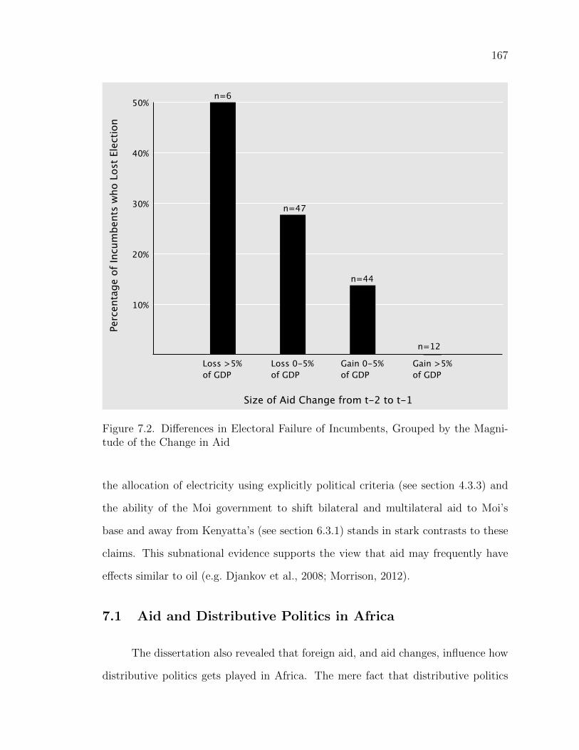
167

Loss >5%of GDP

Loss 0-5%of GDP

Gain 0-5%of GDP

Gain >5%of GDP

50%

10%

20%

30%

40%

Size of Aid Change from t-2 to t-1

Perc

enta

ge o

f In

cum

ben

ts w

ho L

ost

Elec

tion

n=6

n=47

n=44

n=12

Figure 7.2. Di↵erences in Electoral Failure of Incumbents, Grouped by the Magni-tude of the Change in Aid

the allocation of electricity using explicitly political criteria (see section 4.3.3) and

the ability of the Moi government to shift bilateral and multilateral aid to Moi’s

base and away from Kenyatta’s (see section 6.3.1) stands in stark contrasts to these

claims. This subnational evidence supports the view that aid may frequently have

e↵ects similar to oil (e.g. Djankov et al., 2008; Morrison, 2012).

7.1 Aid and Distributive Politics in Africa

The dissertation also revealed that foreign aid, and aid changes, influence how

distributive politics gets played in Africa. The mere fact that distributive politics

168

matters is positive, as it shows that voters are responding to goods and services.

Africans say that providing infrastructure and services as about as important for

politicians as representing the people (Young, 2009), so this should not be surprising.

Still, it serves as a useful counterbalance to the strong emphasis on ethnicity in some

writing on African elections (e.g. Horowitz, 1985).

Aside from counterbalancing interpretations that emphasize ethnicity, the dis-

sertation also showed how politicians respond to the pressure for better infrastructure

or services. Here it seems that aid influences election outcomes in di↵erent ways de-

pending on the pre-existing domestic institutions in the country. This idea has clear

echoes of Burnside and Dollar (2000), but its claim is smaller. Burnside and Dol-

lar (2000) argued that foreign aid could boost growth, but only if it was spent in

countries with good policies and institutions. Their findings have since been called

into question (Easterly et al., 2004), but the fundamental idea of the work—that

international forces must filter through domestic institutions before shaping domes-

tic outcomes—remains persuasive. In the present work, aid changes clearly interact

with domestic politics and these complex interactions determine how much of an

influence aid changes have on electoral outcomes. While political factors seemed to

matter in Ghanaian electricity allocation, they mattered less than technocratic fac-

tors. While aid for electricity bought the NDC votes in Ghana, aid-funded electricity

had widespread benefits throughout the country. This is expected when politicians

try to influence a fairly broad cross-section of voters through the provision of local

public goods (Diaz-Cayeros and Magaloni, 2003). While checks on presidential power

were weak in Ghana, they were far weaker in Kenya (Kivuva, 2011). This led to more

narrow targeting of local public goods in Kenya, and Moi’s regions were the main

beneficiaries.

The di↵erence between Ghanaian allocations and Kenyan allocations is poorly

169

explained by the actions of foreign donors. Kenya was under closer donor scrutiny

than Ghana, but in Kenya local political calculations dominated allocations while

in Ghana political calculations were balanced by technocratic ones. While donor

policies or incentives cannot explain this variation, domestic institutions in recipient

countries can. Domestic political institutions also explain the case of Malawi, where

we find blatant corruption around aid for school construction. This is surprising if

we think purely about the donor side, but it makes more sense when one realizes

that this form of corruption (based around contract procurement) was a hallmark

of the Muluzi period (Cammack and Kelsall, 2011). On average, aid increases help

incumbent presidents and aid decreases hurt them, because aid makes up some of

the resources that politicians can use to provide goods and services to retrospective

voters. However, the ways that those goods or services are provided are practically

important and hinge far more on domestic institutions than on donor actions. Thus,

while donors can change the level of foreign resources provided to politicians, they

are less likely to be able to influence the incentive structures that determine how

money is spent. A practical donor will acknowledge a stronger role for domestic

incentive structures in recipient countries and strive to operate within local incentive

structures instead of striving to change them. This seems to be the trend amongst

rising donors such as China (Brautigam, 2009). This view is also reflected in recent

re-evaluations of governance and foreign aid by practitioner researchers (e.g. Booth,

2011; Institute of Development Studies, 2011). These arguments stress using existing

recipient institutions as a crucial starting point and finding ways to work within them,

even while pushing for marginal change. Finally, the primacy of recipient institutions

can also be read as placing more emphasis on selectivity (the selection of recipients)

over conditionality (attempts to shift incentive structures).1

1While the call for selectivity over conditionality is not new, it has also been largely ignoredand could use reinforcement (Clist, 2011).

170

7.2 Foreign aid and Democracy

While domestic institutions are critically important to explaining election out-

comes, the present work has focused on international forces. This is because aid

volatility is a serious problem, and fluctuations in the foreign aid system filter down

to influence how politics is played in aid recipients. Aid cuts, driven by domestic pol-

itics in donor countries, likely influence election outcomes in recipients. The degree

of influence that aid changes have on election outcomes is driven by the magnitude

of the aid change and domestic political configurations in the aid recipient, but these

e↵ects are real and measurable. In Ghana in 2000, for example, the incumbent NDC

government gained seven more percentage points of the vote in the constituencies

that received an aid project. Theoretically, this is an instance of second-image re-

versed relationship (Gourevitch, 1978), where international forces shape domestic

politics. While this theoretical relationship is interesting, the main findings have

practical implications as well.

The most obvious practical finding is that aid volatility is worse than was

previously thought. Not only do aid changes potentially spark civil wars (Nielsen

et al., 2011) and decrease growth (Lensink and Morrissey, 2000), they also exert

an influence over recipient politics and influence electoral outcomes. The idea that

domestic politics drives aid changes can be seen in current events. For example, the

EU recently reached a budget deal that froze EU aid at current levels (Rosenkranz,

2013). Previous slowdowns in the 1990s led to large aid cuts of over 10% (Frot,

2009). These aid cuts have real implications for political competition in aid-recipient

countries.

This does not, however, mean that aid changes reduce the degree of choice

available to African voters. Instead, it means that aid recipients are part of a system

where the goods and services that influence voters are subject to more uncertainty

171

and greater volatility than similar goods and services in high income countries. Voters

in both high and low income countries often make retrospective calculations when

voting. However, in aid recipient countries politicians are more likely to be punished

or rewarded for random changes in aid.

This means that aid volatility is likely to contribute to a structure where

recipient country politicians find it more di�cult to use feedback from elections or

the economy to learn about the e↵ect of policies. The same learning problem is true

of voters, who likely do not (and probably cannot) distinguish between the e↵ects of

the policies of a president and the e↵ect of aid volatility. This is a problem with any

dependence on a single volatile stream of revenue, and is much more of a problem

with oil (Collier, 2007, Chapter 3). Though aid dependence is often—though not

always—less of a problem than oil dependence, the volatility inherent in both may

prevent learning and reduce the ability of electoral feedback to generate good policies.

This concern has not been adequately voiced in discussions of democratization in aid

recipient countries. It also has not been raised in the discussion on aid volatility.

7.3 Closing thoughts

This dissertation has presented a theoretical argument for why changes in aid

will influence incumbent advantage in Africa. Aid changes influence the level of goods

and services that politicians can provide to voters. This matters because voters are

sensitive to short-term changes in their standard of living and these changes influence

vote choices. The influence of aid changes is practically important because aid is

highly volatile. While changes in aid influence incumbent advantage on average,

the e↵ect of aid changes in specific case will hinge on domestic institutions and in

particular, the level of constraint on recipient presidents. Where presidents have

fewer constraints, they can amplify the e↵ect of an aid increase and reduce the e↵ect

172

of an aid decrease. More highly constrained presidents will have fewer options for

a↵ecting the magnitude of the e↵ect of aid changes.

In particular cases, the form of aid interacts with discretion to produce distinct

pathways between aid changes in voter choices. Case studies in Ghana and Malawi

traced out the two main pathways: the provision of (local) public goods and the

provision of private goods. Aid-funded electricity was provided to voters in Ghana

and roads and education were provided in Malawi and incumbents did better in the

places that received these resources. In Kenya, the president was able to blunt the

e↵ect of an aid cut that was specifically aimed at forcing an election (and for some

donors, removing him from power) by exercising extreme discretion. The specific

form of aid and local domestic political contexts determine how aid is targeted. In

Ghana politicians exercised discretion by directing aid at leaning swing areas. In

Malawi and Kenya discretion was used to direct aid to core supporters. Regardless

of the specific linkages, across cases we find a similar pattern: volatile aid leads to

volatility in the provision of goods and services and this impacts the likelihood that

an aid-recipient president will be re-elected.

173

APPENDIX A

AN AGENT-BASED MODEL OF

THE AID SYSTEM

A.1 Aid Volatility and Agent-Based Models

The aid system is highly volatile, and this dissertation examined the influence

of aid changes on incumbent advantage.1 This appendix presents a simple agent-

based model (ABM) which demonstrates that relatively small changes in the factors

that drive donor decision making can aggregate into large changes in aid from the

point of view of individual aid recipients, and that this can happen even if donors

do not act in concert. This is important because while the current aid system has a

great deal of volatility (Bulir and Hamann, 2008), the sources of that volatility are

understudied. The model in this appendix shows that it is plausible that most of the

volatility in the aid system results from individual, uncoordinated donors actions.

This matters because if the model failed to produce accurate systemic results, then

it would suggest that the underlying assumptions (that individual donors acting

independently can produce systemic volatility) were not logically consistent. I quickly

summarize what we know empirically about aid volatility and then explain the basics

1This appendix contains only a short summary of the research on aid volatility. For moreinformation see the discussion in Section 1.2.

174

of agent-based modeling and the I present presen the model and some output. The

appendix concludes by drawing some additional lessons from the simulation.

A.1.1 Why Does Aid Volatility Exist

There is only one empirical study of the causes of aid volatility (Kharas and

Desai, 2010). This study found that recipient characteristics (regime type, position-

ing on the political spectrum, the presence of elections) were largely unimportant

in explaining volatility.2 Volatility at the recipient level was much better explained

by characteristics such as the type of ‘aid portfolio’ that recipients held. Aid recipi-

ents with less diverse donor portfolios—where one or two donors gave most of their

aid—tended to see more volatility than recipients with diverse portfolios.3 Donors

also were not all alike, with the US emerging as the most volatile aid giver and the

multilaterals emerging as the least. The authors of the study conclude that donor

coordination is part of the problem, and that “the current system of proliferating

donors and projects with lumpy shifts in aid is too clumsy to achieve smooth resource

transfers” (Kharas and Desai, 2010, p. 24).

In the dissertation, I worked on the assumption that donors are not generally

coordinating their annual aid increases or decreases. I also worked under the as-

sumption that changes in aid budgets are usually based on domestic politics in the

donor country and are generally not based on the actions of individual recipients.

This is a useful assumption, because it allows me to cast a more causal interpretation

on the statistical results from Chapter 3.4 The case studies generally support the

2The only exception was that the authors found that aid-dependence and the presence ofinternal violence or adverse regime changes were statistically significant predictors of increases inaid volatility.

3This supports the idea that donors often give aid in an uncoordinated fashion. This will beexamined further on in the model.

4Chapter 3 shows that aid recipients that experience aid increases in the year before anelection are more likely to see their incumbent presidents win re-election than the recipients that

175

argument that, from the point of view of most aid recipients, most aid changes are

random. The decline in aid to Ghana in Chapter 4 was not based on anything that

Ghana did and the aid increase to Malawi in Chapter 5 was similarly detached from

any actions on the part of the government of Malawi. While individual donors surely

had their reasons for increasing or decreasing aid, most seem to have been driven by

a mixture of unique domestic motives. Also, in general, the per-donor changes were

small. That these small changes in aid cumulated into large aid swings before an

election was simply bad luck. The obvious exception to this pattern is Chapter 6, but

Kenya was picked because it was an exception. This appendix cannot conclusively

demonstrate that most aid changes are driven by stochastic factors, but it can show

that the when donors are modeled in this way, the outcome is a broadly realistic

level of aid volatility and realistic patterns of aid over time and the recipient level.

A.1.2 Why Model?

Agent-based modeling (ABM) is relatively new in the social sciences, but it has

a number of advantages that make it worth pursuing. The first advantage applies to

all mathematical models, and it is that it allows the researcher to rigorously describe

one simplification of the world. The very act of programming an ABM forces one to

be explicit about their mental model of how the world works. The second advantage

is that it can test the logical consistency of an argument. This can be done in two

ways. First, by producing a world with agents that interact over time and then

letting the world unfold, the modeler can show that a given specification of agents

can produce an outcome of interest. In the words of Epstein (1999, p. 42), “agent-

based models provide computational demonstrations that a given microspecification

is in fact su�cient to generate a macrostructure of interest.” The second approach to

testing the logical consistency of an argument with an ABM is by examining how the

see aid decreases in the year before their election.

176

macrostructure changes when agents are given extreme values on certain variables.5

This can help to show the points at which certain macrostructures break down and

it can also critique a theory if the macrostructure of interest is produced from wildly

implausible agent microspecifications.

Here I use an ABM to test if my assumptions about donor actions are plausible.

This dissertation tends to view donors as poorly coordinated and acting on a fairly

steady mixture of altruism and strategic interests. It posits that outside shocks that

make a recipient more needy (like a famine) or more strategically important will

drive changes in aid between specific donors and recipients, but that the aid system

itself will have a certain base level of volatility due to many donors making small,

uncoordinated changes to their aid budgets each year. These sorts of assumptions

may sound plausible, but actually modeling them o↵ers a test to see if they form

one set of donor rules that can produce realistic-looking aggregate data on measures

such as systemic aid volatility. While this does not show that this set of donor rules

actually matches the rules of donors in the real world, it does show logical su�ciency

and should increase our confidence in the logical foundations on which the discussion

of the political e↵ects of aid volatility rests.

A.1.3 Testing Models

If we accept the previous remarks and think that ABMs can be useful, the next

issue is how to test them. Models are typically tested on their ability to produce

macro-level patterns of interest. Precisely which pattern and how closely it should

match reality depends on the goal of the model. Some models are very abstract and

are meant to show general tendencies than can be applied to diverse situations. A

famous example of this is the Game of Life (Conway, 1970). In international relations,

the best example would be the prisoner’s dilemma tournaments hosted by Axelrod

5This is known as a sensitivity analysis.

177

(1997). These models are generally accepted as ideal-type logical experiments and are

usually not judged by their ability to represent reality. Slightly less abstract models,

such as Schelling’s (1969) ABM of segregation, aim at capturing one abstract sliver

of reality. More detailed models often incorporate many heterogeneous agents with

very complicated interaction rules and very complicated terrain. Cio�-Revilla and

Rouleau (2010) present one such model which shows the rise and decline of polities

and includes dynamic weather and a broad array of social and political interactions

between agents. Finally, at the far end of the spectrum are models that are carefully

calibrated using real-world data and use GIS to allow the agents to interact on

representations of the physical world. Hailegiorgis et al. (2010) present one such

model attempting to explain and eventually predict conflicts between herders around

watering holes in East Africa.

Gilbert (2008) gives advice on testing model validity. General models are tested

based on their ability to shed light on general concepts of interest. These models,

like Conway’s Game of Life, aim more at elegance and fertility than prediction or

explanation of specific events. They should be judged according to these criteria.

Detailed, or “facsimile,” models that aim to explain specific events are often tested

based on the model’s ability to represent the empirical patterns under question.

My model is a middle-range model, similar in scope to Schelling’s segregation model.

Gilbert recommends that these models are tested against their ability to produce the

broad patterns under question. He also recommends testing ABMs with a sensitivity

analysis. This is especially useful if empirical data are sparse, because it can show if

the model is constructed such that it breaks down when extreme but plausible levels

of variables are given to agents.6

6Just as troubling, it could also reveal that the model produces reliable results when agentsare given outrageously large or small levels for key variables.

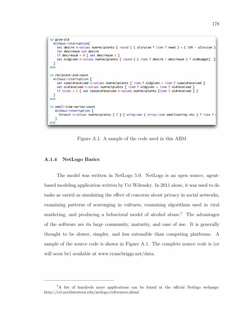
178

Figure A.1. A sample of the code used in this ABM

A.1.4 NetLogo Basics

The model was written in NetLogo 5.0. NetLogo is an open source, agent-

based modeling application written by Uri Wilensky. In 2011 alone, it was used to do

tasks as varied as simulating the e↵ect of concerns about privacy in social networks,

examining patterns of scavenging in vultures, examining algorithms used in viral

marketing, and producing a behavioral model of alcohol abuse.7 The advantages

of the software are its large community, maturity, and ease of use. It is generally

thought to be slower, simpler, and less extensible than competing platforms. A

sample of the source code is shown in Figure A.1. The complete source code is (or

will soon be) available at www.ryancbriggs.net/data.

7A list of hundreds more applications can be found at the o�cial Netlogo webpage:http://ccl.northwestern.edu/netlogo/references.shtml

179

A.1.5 Motivations behind the model

This Chapter presents a simple mode of how donors decide to allocate aid. It

then uses the model to show how small changes in the factors that influence donor

decision making aggregate into a very uncertain aid environment from the point of

view of aid recipients. The model will be discussed in much more detail below, but it

is useful now to describe the intuition behind the model, as well as its basic building

blocks and how they fit together.

While in the current world there are some aid recipients—like India—who also

are donors, in the model there are only donors or recipients.8 Each recipient has a

degree of need for aid. This ‘need’ value is a simplification that should be understood

as aggregating everything that could potentially be improved by aid, from education

to infrastructure. One would expect that the need score would correspond closely

to GDP per capita, for example, and that in the real world Malawi would have a

higher need score than Kenya. Each donor has three attributes. First, they all have

a measure of strategic importance that they attach to each individual recipient. This

means that while each donor would see Senegal as equally in need of assistance, they

would not all see it as equally strategically important. In the Senegalese example, it

is likely that the French would find Senegal more strategically important than would

the United States. Donors also have an aid budget that they allocate amongst the

recipients, and each donor’s aid budget is a di↵erent size. Finally, donors have a

measure of altruism. This is used to help them decide between allocating their fixed

aid budget according to strategic concerns or recipient need. While this is also a

simplification, it reflects a broad pattern in the current world, where some donors

(like the Nordics) seem to respond more to recipient need and other donors (the US,

8The model does, however, represent donors like India if we believe that these countries donot consider how much aid they will receive from others when they calculate how they will disburse.

180

France, China) seem to respond more to the strategic importance of a country.

A.1.6 Macrocharacteristics of the aid system

This section explains the ways that the model will be judged. Being a middle-

range model, the goal here is to see if the agent-rules that I have broadly outlined

above and rigorously specify in Section A.2 will produce macro-level patterns that

are broadly similar to real world data. In my specific instance, I want to produce:

1. An approximation of the mean level of aid volatility across all recipients in the

system,

2. An approximation of realistic aid volatility at the recipient level,

3. A system where more strategic voters have a higher level of variance in aid giving

than more altruistic donors, as shown in Kharas and Desai (2010),

4. A system where increases in the number of donors per recipient reduces volatility,

again as shown in Kharas and Desai (2010).

I am not aiming to capture any patterns in aid to specific countries and I am

not modeling any specific pattern of relationships between actual countries. Instead

the model aims only to at general patterns. It does, however, aim to produce realistic

patterns at both the level of the aid system and at the level of the individual recipient

over time. The goal is to see if my assumptions about donor behavior are su�cient

to generate realistic patterns in aid volatility. The next section describes how these

general goals are translated into specific code.

A.2 The Setup of the Model

This section describes the model in detail. Every model is broadly divided

into two sections: initialization and the simulation loop. The former is the setup

181

phase of the model and the latter is the recurring set of decisions that the agents

make in each turn of the simulation. First, I describe the setup phase. The model

includes two kinds of actors: donors and recipients.9 The number of donors and

recipients is set by the user and is capped at 50 and 100, respectively. As discussed

before, each donor has three attributes: an aid budget, an altruism score, and a list

of values reflecting their strategic interest in each recipient. Recipients have only one

attribute, which reflects how much they need aid.10 The only potentially confusing

aspect of this model is that while each recipient has a need variable and each donor

has an aid budget variable or an altruism variable, each donor-recipient pair has

its own strategic interest variable. Again, this reflects the fact that while all donors

would likely agree on how much a given country needs aid, they would not necessarily

agree on its strategic importance.

In the setup phase of the model, donors are randomly assigned values for

their aid budget, altruism, and strategic interest in each recipient, and recipients are

randomly assigned a need variable. A full description of these variables is provided

in Table 1.1.

The need, strategic, and aidbudget variables are all set according to an exponen-

tial distribution. The reflects current realities, where aid budgets, aid requirements,

or the strategic importance of countries vary widely and non-normally. Altruism was

set according to a normal distribution. While these choices help to create output

that more closely resembles actual aid allocations, they are not needed to replicate

the main finding of the model. Once the simulation has been initialized it then loops

for 50 turns, roughly representing the choices that donors make when allocating aid

9Only donors are actually modeled as agents. Recipients are each assigned a number. Thishas no e↵ect on the results of the model but greatly simplifies the code.

10The model requires many more variables than are discussed here. The variables discussedhere form the theoretical core of the model. The remaining variables exist to make calculations andsave output.

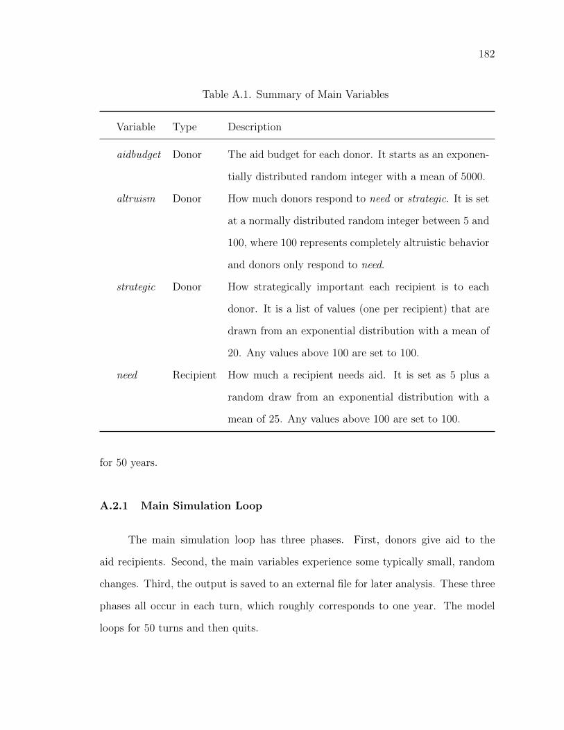
182

Table A.1. Summary of Main Variables

Variable Type Description

aidbudget Donor The aid budget for each donor. It starts as an exponen-

tially distributed random integer with a mean of 5000.

altruism Donor How much donors respond to need or strategic. It is set

at a normally distributed random integer between 5 and

100, where 100 represents completely altruistic behavior

and donors only respond to need.

strategic Donor How strategically important each recipient is to each

donor. It is a list of values (one per recipient) that are

drawn from an exponential distribution with a mean of

20. Any values above 100 are set to 100.

need Recipient How much a recipient needs aid. It is set as 5 plus a

random draw from an exponential distribution with a

mean of 25. Any values above 100 are set to 100.

for 50 years.

A.2.1 Main Simulation Loop

The main simulation loop has three phases. First, donors give aid to the

aid recipients. Second, the main variables experience some typically small, random

changes. Third, the output is saved to an external file for later analysis. These three

phases all occur in each turn, which roughly corresponds to one year. The model

loops for 50 turns and then quits.

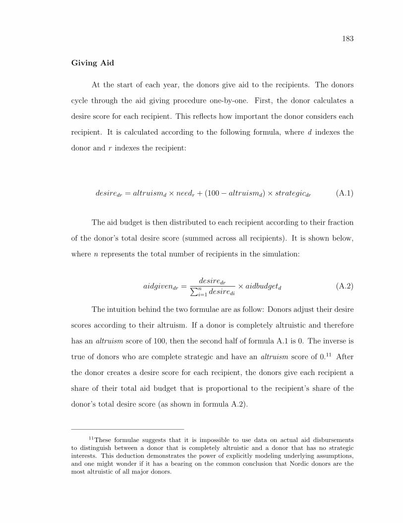
183

Giving Aid

At the start of each year, the donors give aid to the recipients. The donors

cycle through the aid giving procedure one-by-one. First, the donor calculates a

desire score for each recipient. This reflects how important the donor considers each

recipient. It is calculated according to the following formula, where d indexes the

donor and r indexes the recipient:

desiredr = altruismd ⇥ needr + (100� altruismd)⇥ strategicdr (A.1)

The aid budget is then distributed to each recipient according to their fraction

of the donor’s total desire score (summed across all recipients). It is shown below,

where n represents the total number of recipients in the simulation:

aidgivendr =desiredrPni=1 desiredi

⇥ aidbudgetd (A.2)

The intuition behind the two formulae are as follow: Donors adjust their desire

scores according to their altruism. If a donor is completely altruistic and therefore

has an altruism score of 100, then the second half of formula A.1 is 0. The inverse is

true of donors who are complete strategic and have an altruism score of 0.11 After

the donor creates a desire score for each recipient, the donors give each recipient a

share of their total aid budget that is proportional to the recipient’s share of the

donor’s total desire score (as shown in formula A.2).

11These formulae suggests that it is impossible to use data on actual aid disbursementsto distinguish between a donor that is completely altruistic and a donor that has no strategicinterests. This deduction demonstrates the power of explicitly modeling underlying assumptions,and one might wonder if it has a bearing on the common conclusion that Nordic donors are themost altruistic of all major donors.

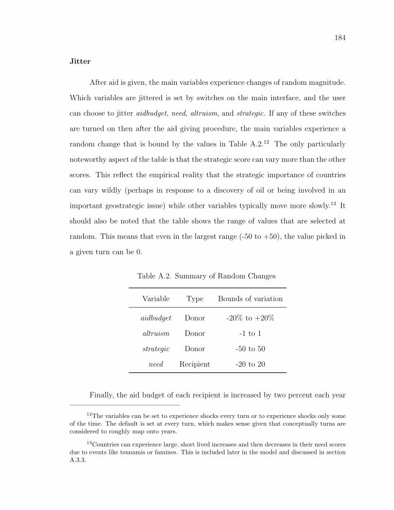
184

Jitter

After aid is given, the main variables experience changes of random magnitude.

Which variables are jittered is set by switches on the main interface, and the user

can choose to jitter aidbudget, need, altruism, and strategic. If any of these switches

are turned on then after the aid giving procedure, the main variables experience a

random change that is bound by the values in Table A.2.12 The only particularly

noteworthy aspect of the table is that the strategic score can vary more than the other

scores. This reflect the empirical reality that the strategic importance of countries

can vary wildly (perhaps in response to a discovery of oil or being involved in an

important geostrategic issue) while other variables typically move more slowly.13 It

should also be noted that the table shows the range of values that are selected at

random. This means that even in the largest range (-50 to +50), the value picked in

a given turn can be 0.

Table A.2. Summary of Random Changes

Variable Type Bounds of variation

aidbudget Donor -20% to +20%

altruism Donor -1 to 1

strategic Donor -50 to 50

need Recipient -20 to 20

Finally, the aid budget of each recipient is increased by two percent each year

12The variables can be set to experience shocks every turn or to experience shocks only someof the time. The default is set at every turn, which makes sense given that conceptually turns areconsidered to roughly map onto years.

13Countries can experience large, short lived increases and then decreases in their need scoresdue to events like tsunamis or famines. This is included later in the model and discussed in sectionA.3.3.

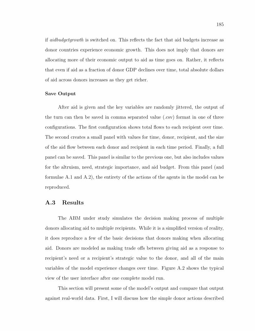
185

if aidbudgetgrowth is switched on. This reflects the fact that aid budgets increase as

donor countries experience economic growth. This does not imply that donors are

allocating more of their economic output to aid as time goes on. Rather, it reflects

that even if aid as a fraction of donor GDP declines over time, total absolute dollars

of aid across donors increases as they get richer.

Save Output

After aid is given and the key variables are randomly jittered, the output of

the turn can then be saved in comma separated value (.csv) format in one of three

configurations. The first configuration shows total flows to each recipient over time.

The second creates a small panel with values for time, donor, recipient, and the size

of the aid flow between each donor and recipient in each time period. Finally, a full

panel can be saved. This panel is similar to the previous one, but also includes values

for the altruism, need, strategic importance, and aid budget. From this panel (and

formulae A.1 and A.2), the entirety of the actions of the agents in the model can be

reproduced.

A.3 Results

The ABM under study simulates the decision making process of multiple

donors allocating aid to multiple recipients. While it is a simplified version of reality,

it does reproduce a few of the basic decisions that donors making when allocating

aid. Donors are modeled as making trade o↵s between giving aid as a response to

recipient’s need or a recipient’s strategic value to the donor, and all of the main

variables of the model experience changes over time. Figure A.2 shows the typical

view of the user interface after one complete model run.

This section will present some of the model’s output and compare that output

against real-world data. First, I will discuss how the simple donor actions described

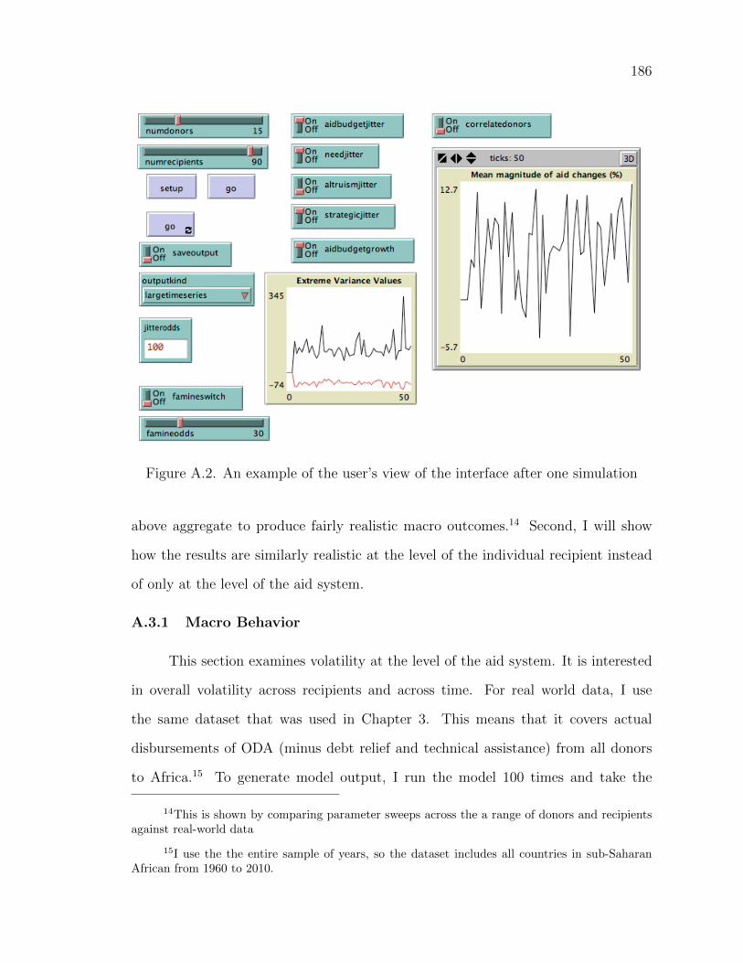
186

Figure A.2. An example of the user’s view of the interface after one simulation

above aggregate to produce fairly realistic macro outcomes.14 Second, I will show

how the results are similarly realistic at the level of the individual recipient instead

of only at the level of the aid system.

A.3.1 Macro Behavior

This section examines volatility at the level of the aid system. It is interested

in overall volatility across recipients and across time. For real world data, I use

the same dataset that was used in Chapter 3. This means that it covers actual

disbursements of ODA (minus debt relief and technical assistance) from all donors

to Africa.15 To generate model output, I run the model 100 times and take the

14This is shown by comparing parameter sweeps across the a range of donors and recipientsagainst real-world data

15I use the the entire sample of years, so the dataset includes all countries in sub-SaharanAfrican from 1960 to 2010.

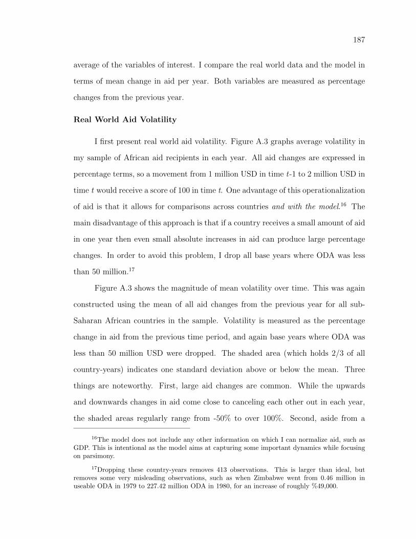
187

average of the variables of interest. I compare the real world data and the model in

terms of mean change in aid per year. Both variables are measured as percentage

changes from the previous year.

Real World Aid Volatility

I first present real world aid volatility. Figure A.3 graphs average volatility in

my sample of African aid recipients in each year. All aid changes are expressed in

percentage terms, so a movement from 1 million USD in time t-1 to 2 million USD in

time t would receive a score of 100 in time t. One advantage of this operationalization

of aid is that it allows for comparisons across countries and with the model.16 The

main disadvantage of this approach is that if a country receives a small amount of aid

in one year then even small absolute increases in aid can produce large percentage

changes. In order to avoid this problem, I drop all base years where ODA was less

than 50 million.17

Figure A.3 shows the magnitude of mean volatility over time. This was again

constructed using the mean of all aid changes from the previous year for all sub-

Saharan African countries in the sample. Volatility is measured as the percentage

change in aid from the previous time period, and again base years where ODA was

less than 50 million USD were dropped. The shaded area (which holds 2/3 of all

country-years) indicates one standard deviation above or below the mean. Three

things are noteworthy. First, large aid changes are common. While the upwards

and downwards changes in aid come close to canceling each other out in each year,

the shaded areas regularly range from -50% to over 100%. Second, aside from a

16The model does not include any other information on which I can normalize aid, such asGDP. This is intentional as the model aims at capturing some important dynamics while focusingon parsimony.

17Dropping these country-years removes 413 observations. This is larger than ideal, butremoves some very misleading observations, such as when Zimbabwe went from 0.46 million inuseable ODA in 1979 to 227.42 million ODA in 1980, for an increase of roughly %49,000.

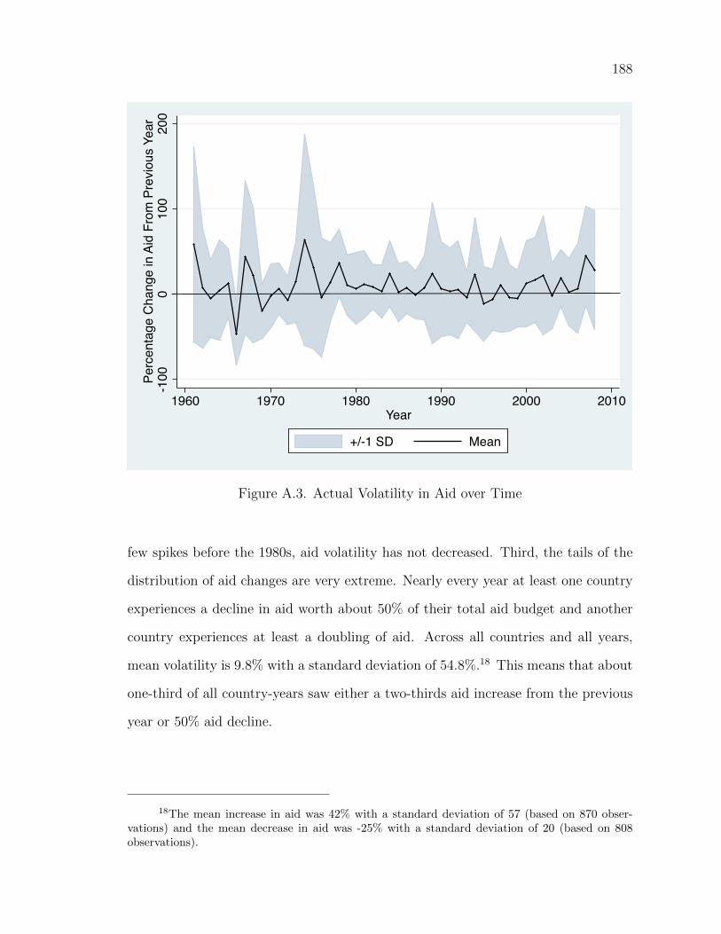
188

-100

010

020

0Pe

rcen

tage

Cha

nge

in A

id F

rom

Pre

viou

s Ye

ar

1960 1970 1980 1990 2000 2010Year

+/-1 SD Mean

Figure A.3. Actual Volatility in Aid over Time

few spikes before the 1980s, aid volatility has not decreased. Third, the tails of the

distribution of aid changes are very extreme. Nearly every year at least one country

experiences a decline in aid worth about 50% of their total aid budget and another

country experiences at least a doubling of aid. Across all countries and all years,

mean volatility is 9.8% with a standard deviation of 54.8%.18 This means that about

one-third of all country-years saw either a two-thirds aid increase from the previous

year or 50% aid decline.

18The mean increase in aid was 42% with a standard deviation of 57 (based on 870 obser-vations) and the mean decrease in aid was -25% with a standard deviation of 20 (based on 808observations).

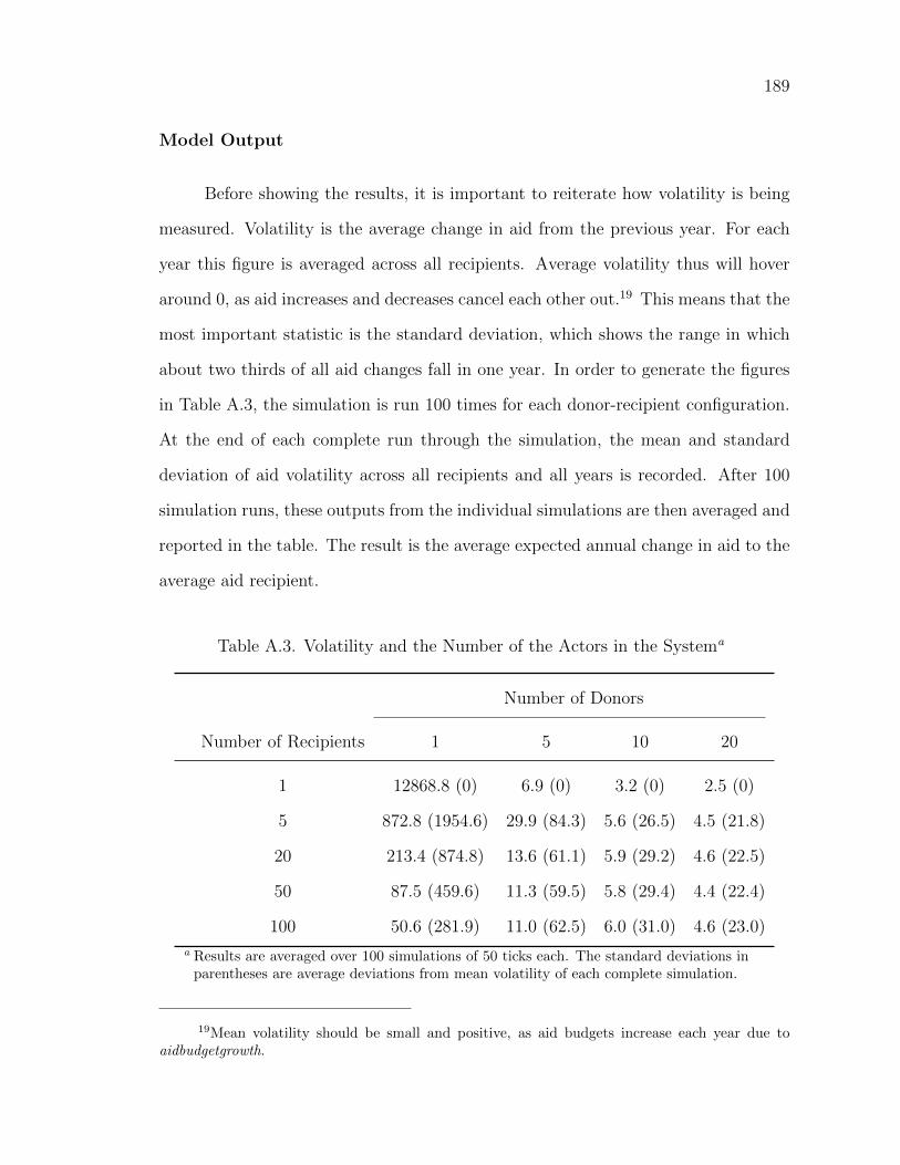
189

Model Output

Before showing the results, it is important to reiterate how volatility is being

measured. Volatility is the average change in aid from the previous year. For each

year this figure is averaged across all recipients. Average volatility thus will hover

around 0, as aid increases and decreases cancel each other out.19 This means that the

most important statistic is the standard deviation, which shows the range in which

about two thirds of all aid changes fall in one year. In order to generate the figures

in Table A.3, the simulation is run 100 times for each donor-recipient configuration.

At the end of each complete run through the simulation, the mean and standard

deviation of aid volatility across all recipients and all years is recorded. After 100

simulation runs, these outputs from the individual simulations are then averaged and

reported in the table. The result is the average expected annual change in aid to the

average aid recipient.

Table A.3. Volatility and the Number of the Actors in the Systema

Number of Donors

Number of Recipients 1 5 10 20

1 12868.8 (0) 6.9 (0) 3.2 (0) 2.5 (0)

5 872.8 (1954.6) 29.9 (84.3) 5.6 (26.5) 4.5 (21.8)

20 213.4 (874.8) 13.6 (61.1) 5.9 (29.2) 4.6 (22.5)

50 87.5 (459.6) 11.3 (59.5) 5.8 (29.4) 4.4 (22.4)

100 50.6 (281.9) 11.0 (62.5) 6.0 (31.0) 4.6 (23.0)

a Results are averaged over 100 simulations of 50 ticks each. The standard deviations inparentheses are average deviations from mean volatility of each complete simulation.

19Mean volatility should be small and positive, as aid budgets increase each year due toaidbudgetgrowth.

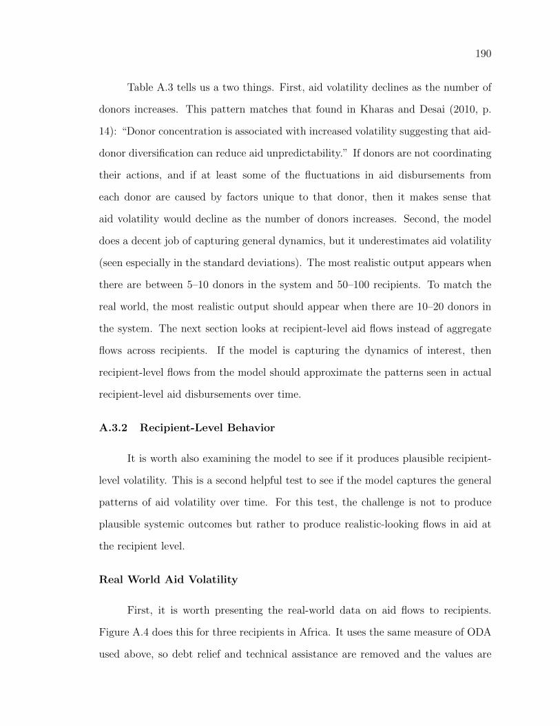
190

Table A.3 tells us a two things. First, aid volatility declines as the number of

donors increases. This pattern matches that found in Kharas and Desai (2010, p.

14): “Donor concentration is associated with increased volatility suggesting that aid-

donor diversification can reduce aid unpredictability.” If donors are not coordinating

their actions, and if at least some of the fluctuations in aid disbursements from

each donor are caused by factors unique to that donor, then it makes sense that

aid volatility would decline as the number of donors increases. Second, the model

does a decent job of capturing general dynamics, but it underestimates aid volatility

(seen especially in the standard deviations). The most realistic output appears when

there are between 5–10 donors in the system and 50–100 recipients. To match the

real world, the most realistic output should appear when there are 10–20 donors in

the system. The next section looks at recipient-level aid flows instead of aggregate

flows across recipients. If the model is capturing the dynamics of interest, then

recipient-level flows from the model should approximate the patterns seen in actual

recipient-level aid disbursements over time.

A.3.2 Recipient-Level Behavior

It is worth also examining the model to see if it produces plausible recipient-

level volatility. This is a second helpful test to see if the model captures the general

patterns of aid volatility over time. For this test, the challenge is not to produce

plausible systemic outcomes but rather to produce realistic-looking flows in aid at

the recipient level.

Real World Aid Volatility

First, it is worth presenting the real-world data on aid flows to recipients.

Figure A.4 does this for three recipients in Africa. It uses the same measure of ODA

used above, so debt relief and technical assistance are removed and the values are

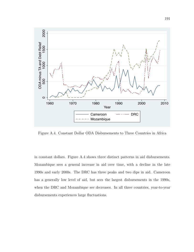
191

050

010

0015

0020

00O

DA m

inus

TA

and

Debt

Rel

ief

1960 1970 1980 1990 2000 2010Year

Cameroon DRCMozambique

Figure A.4. Constant Dollar ODA Disbursements to Three Countries in Africa

in constant dollars. Figure A.4 shows three distinct patterns in aid disbursements.

Mozambique sees a general increase in aid over time, with a decline in the late

1990s and early 2000s. The DRC has three peaks and two dips in aid. Cameroon

has a generally low level of aid, but sees the largest disbursements in the 1990s,

when the DRC and Mozambique see decreases. In all three countries, year-to-year

disbursements experiences large fluctuations.

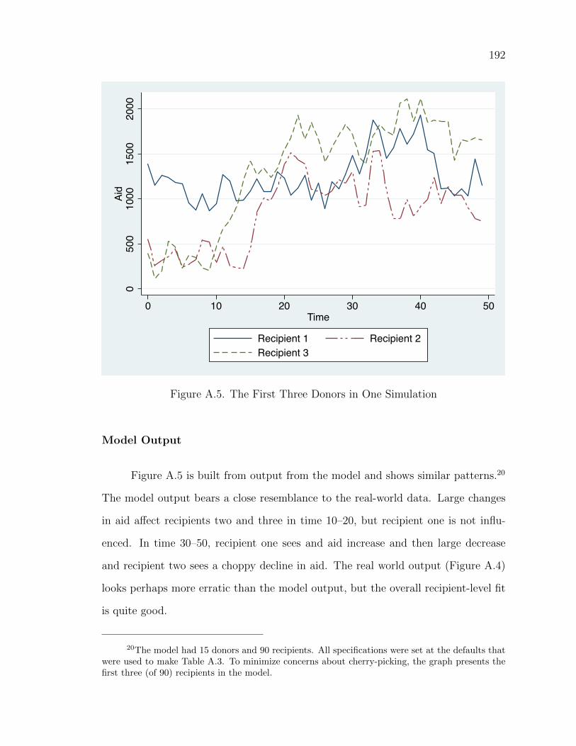
192

050

010

0015

0020

00Ai

d

0 10 20 30 40 50Time

Recipient 1 Recipient 2Recipient 3

Figure A.5. The First Three Donors in One Simulation

Model Output

Figure A.5 is built from output from the model and shows similar patterns.20

The model output bears a close resemblance to the real-world data. Large changes

in aid a↵ect recipients two and three in time 10–20, but recipient one is not influ-

enced. In time 30–50, recipient one sees and aid increase and then large decrease

and recipient two sees a choppy decline in aid. The real world output (Figure A.4)

looks perhaps more erratic than the model output, but the overall recipient-level fit

is quite good.

20The model had 15 donors and 90 recipients. All specifications were set at the defaults thatwere used to make Table A.3. To minimize concerns about cherry-picking, the graph presents thefirst three (of 90) recipients in the model.

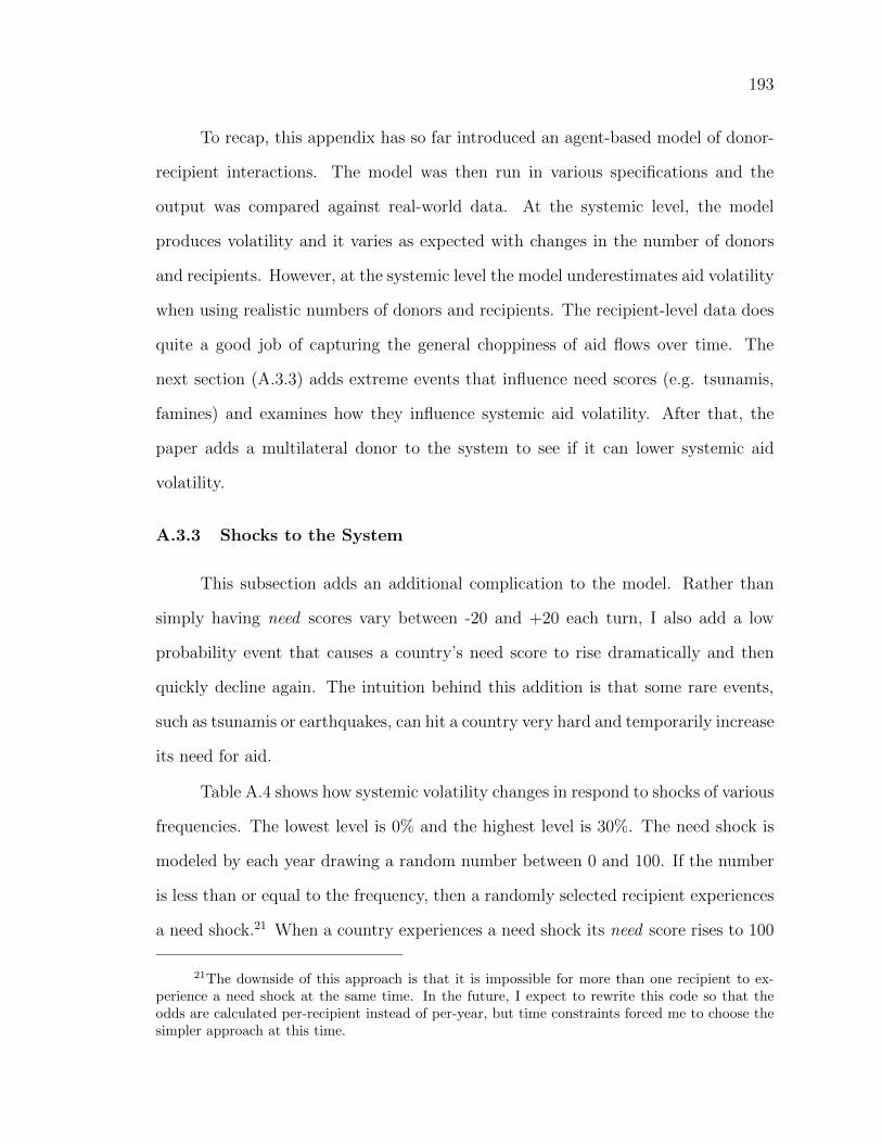
193

To recap, this appendix has so far introduced an agent-based model of donor-

recipient interactions. The model was then run in various specifications and the

output was compared against real-world data. At the systemic level, the model

produces volatility and it varies as expected with changes in the number of donors

and recipients. However, at the systemic level the model underestimates aid volatility

when using realistic numbers of donors and recipients. The recipient-level data does

quite a good job of capturing the general choppiness of aid flows over time. The

next section (A.3.3) adds extreme events that influence need scores (e.g. tsunamis,

famines) and examines how they influence systemic aid volatility. After that, the

paper adds a multilateral donor to the system to see if it can lower systemic aid

volatility.

A.3.3 Shocks to the System

This subsection adds an additional complication to the model. Rather than

simply having need scores vary between -20 and +20 each turn, I also add a low

probability event that causes a country’s need score to rise dramatically and then

quickly decline again. The intuition behind this addition is that some rare events,

such as tsunamis or earthquakes, can hit a country very hard and temporarily increase

its need for aid.

Table A.4 shows how systemic volatility changes in respond to shocks of various

frequencies. The lowest level is 0% and the highest level is 30%. The need shock is

modeled by each year drawing a random number between 0 and 100. If the number

is less than or equal to the frequency, then a randomly selected recipient experiences

a need shock.21 When a country experiences a need shock its need score rises to 100

21The downside of this approach is that it is impossible for more than one recipient to ex-perience a need shock at the same time. In the future, I expect to rewrite this code so that theodds are calculated per-recipient instead of per-year, but time constraints forced me to choose thesimpler approach at this time.

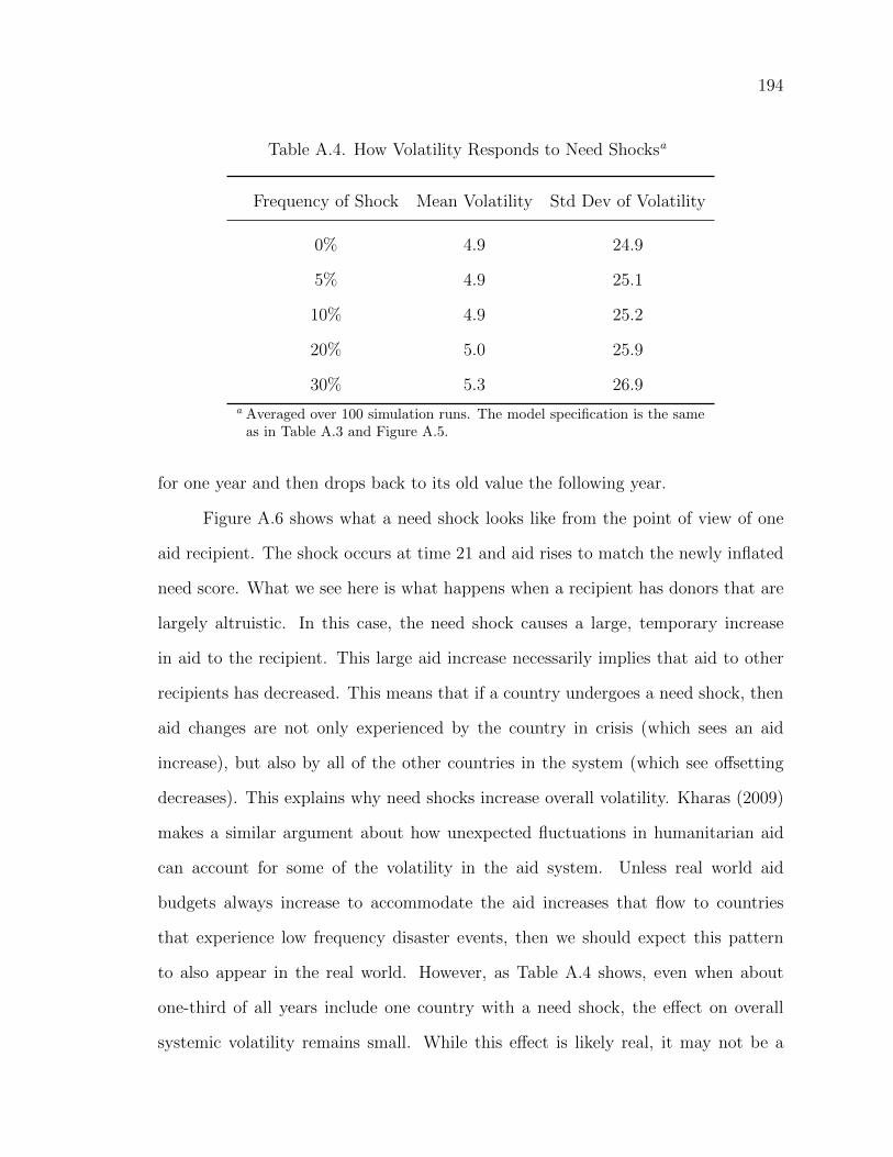
194

Table A.4. How Volatility Responds to Need Shocksa

Frequency of Shock Mean Volatility Std Dev of Volatility

0% 4.9 24.9

5% 4.9 25.1

10% 4.9 25.2

20% 5.0 25.9

30% 5.3 26.9

a Averaged over 100 simulation runs. The model specification is the sameas in Table A.3 and Figure A.5.

for one year and then drops back to its old value the following year.

Figure A.6 shows what a need shock looks like from the point of view of one

aid recipient. The shock occurs at time 21 and aid rises to match the newly inflated

need score. What we see here is what happens when a recipient has donors that are

largely altruistic. In this case, the need shock causes a large, temporary increase

in aid to the recipient. This large aid increase necessarily implies that aid to other

recipients has decreased. This means that if a country undergoes a need shock, then

aid changes are not only experienced by the country in crisis (which sees an aid

increase), but also by all of the other countries in the system (which see o↵setting

decreases). This explains why need shocks increase overall volatility. Kharas (2009)

makes a similar argument about how unexpected fluctuations in humanitarian aid

can account for some of the volatility in the aid system. Unless real world aid

budgets always increase to accommodate the aid increases that flow to countries

that experience low frequency disaster events, then we should expect this pattern

to also appear in the real world. However, as Table A.4 shows, even when about

one-third of all years include one country with a need shock, the e↵ect on overall

systemic volatility remains small. While this e↵ect is likely real, it may not be a

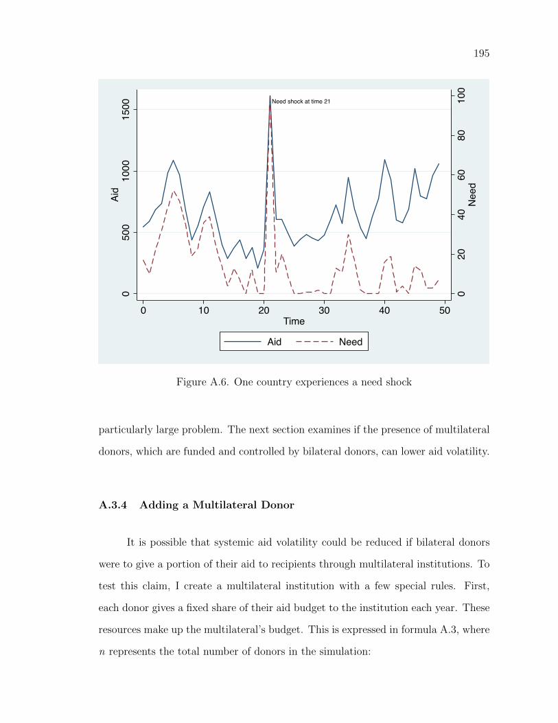
195

Need shock at time 21

020

4060

8010

0N

eed

050

010

0015

00Ai

d

0 10 20 30 40 50Time

Aid Need

Figure A.6. One country experiences a need shock

particularly large problem. The next section examines if the presence of multilateral

donors, which are funded and controlled by bilateral donors, can lower aid volatility.

A.3.4 Adding a Multilateral Donor

It is possible that systemic aid volatility could be reduced if bilateral donors

were to give a portion of their aid to recipients through multilateral institutions. To

test this claim, I create a multilateral institution with a few special rules. First,

each donor gives a fixed share of their aid budget to the institution each year. These

resources make up the multilateral’s budget. This is expressed in formula A.3, where

n represents the total number of donors in the simulation:

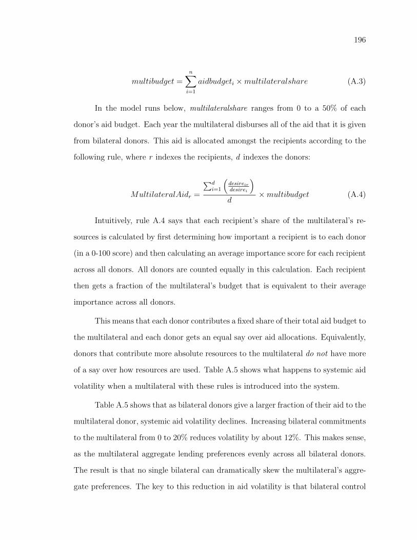
196

multibudget =nX

i=1

aidbudgeti ⇥multilateralshare (A.3)

In the model runs below, multilateralshare ranges from 0 to a 50% of each

donor’s aid budget. Each year the multilateral disburses all of the aid that it is given

from bilateral donors. This aid is allocated amongst the recipients according to the

following rule, where r indexes the recipients, d indexes the donors:

MultilateralAidr =

Pdi=1

⇣desireirdesirei

⌘

d⇥multibudget (A.4)

Intuitively, rule A.4 says that each recipient’s share of the multilateral’s re-

sources is calculated by first determining how important a recipient is to each donor

(in a 0-100 score) and then calculating an average importance score for each recipient

across all donors. All donors are counted equally in this calculation. Each recipient

then gets a fraction of the multilateral’s budget that is equivalent to their average

importance across all donors.

This means that each donor contributes a fixed share of their total aid budget to

the multilateral and each donor gets an equal say over aid allocations. Equivalently,

donors that contribute more absolute resources to the multilateral do not have more

of a say over how resources are used. Table A.5 shows what happens to systemic aid

volatility when a multilateral with these rules is introduced into the system.

Table A.5 shows that as bilateral donors give a larger fraction of their aid to the

multilateral donor, systemic aid volatility declines. Increasing bilateral commitments

to the multilateral from 0 to 20% reduces volatility by about 12%. This makes sense,

as the multilateral aggregate lending preferences evenly across all bilateral donors.

The result is that no single bilateral can dramatically skew the multilateral’s aggre-

gate preferences. The key to this reduction in aid volatility is that bilateral control

197

Table A.5. How Multilateral Donors Influence Aid Volatilitya

Fraction of Donor aidbudget Mean Volatility Standard Deviation

Given to the Multilateral

0% 4.8 25

5% 4.8 24.7

10% 4.5 23.2

15% 4.6 23.7

20% 4.3 22

50% 4.1 21

a Averaged over 100 simulation runs.

over aid allocations is independent of the amount of aid that a donor contributes.

This means that the result collapses if the multilateral weighs votes according to each

bilateral’s share of the multilateral budget. The latter system is in use at the World

Bank, and that reduces the Bank’s ability to combat aid volatility that is based on

external shocks and a lack of donor coordination.

A.4 Conclusion

This appendix created an ABM of donor-recipient interactions and used it

to demonstrate how aid volatility could result from donor’s making uncoordinated

changes in their aid allocations. It also showed how extreme events could increase

aid volatility, even in the countries not a↵ected by the event, and that some properly

structured multilateral institutions could reduce aid volatility.

The model also showed how the act of building a model can reveal aspects

of systems that are often overlooked. In this appendix, formula A.1 suggests that

donors that are completely altruistic and donors that have no strategic interests (but

198

are not very altruistic) will disburse aid in exactly the same manner. This makes it

quite di�cult to ascribe altruistic (non-strategic) intentions to donors that have few

strategic interests. In this formulation, the point seems rather obvious. Still, many

small donors—especially the Nordic countries—are often considered altruistic even

though their potential strategic uses of aid (e.g. Morgenthau, 1962) are limited when

compared to larger donors like the United States or Japan.22

In general, the model does a fairly good job of capturing the general trends

in aid volatility. Specifically, it produces plausible donor-recipient disbursement pat-

terns, plausible recipient-level disbursement patterns, and plausible (though low)

systemic patterns. While this does not show that the model correctly approximates

the actions of donors in the real world, it does show that the assumptions motivating

agent behavior are logical and combine to create a plausible description of one aspect

of the aid system. The model also shows that, in accordance with Kharas and Desai

(2010), aid volatility at both the systemic level and the recipient level declines as

the number of donors increases. So long as donors are acting at least partially on

independent information or are changing their aid budgets based on partially inde-

pendent factors or have di↵erent levels of altruism, then increases in the number

of donors will diminish the overall level of aid volatility in the system.23 For at

least this reason, rising donors such as China, India, or Brazil should be welcomed.

The more their situation di↵ers from the traditional donors, the more likely it is that

their lending can o↵set changes in lending by traditional donors, and thus potentially

smooth year-to-year aid changes.

22For an empirical counterpoint which uses trade data to measure the degree of altruism ina donor, see Berthelemy (2006).

23While this is clearly true, it ignores the issue of aid fragmentation, which is an importantpractical concern and was not considered in this model (Morss, 1984; Knack and Rahman, 2007).

199

REFERENCES

Acemoglu, D., S. Johnson, and J.A. Robinson (2001). “The colonial origins of com-parative development: An empirical exploration.” American Economic Review 91,1369–1401.

Acemoglu, D. and J.A. Robinson (2012). Why nations fail: The origins of power,prosperity, and poverty. Crown Business.

Achen, C. H. and L. M. Bartels (2004). “Blind retrospection: Electoral responses todrought, flu, and shark attacks.” Estudio/Working Paper .

Africa Watch (1993). “Divide and rule: State-sponsored ethnic violence in kenya.”Technical report, Africa Watch, Washington, DC.

Alesina, Alberto and David Dollar (2000). “Who gives foreign aid to whom andwhy?” Journal of Economic Growth 5(1), 33–63.

Alesina, Alberto and B. Weder (2002). “Do corrupt governments receive less foreignaid?” American Economic Review 92(4), 1126–1137.

Andbo, Felix (2001). “The ghana 2000 elections: Voter choice and electoral deci-sions.” African Journal of Political Science 6(1), 69–88.

Atemi, Calem and Buong Arunda (1992, Oct 8). “Kanu has already won – moi.

Aubynn, Anthony Kwesi (2002). “Behind the transparent ballot box: The signifi-cance of the 1990s elections in ghana.” In Michael Cowen and Liisa Laakso, eds.,Multiparty Politics in Africa, Chapter 4, pp. 75–127. New York: Palgrave.

Axelrod, R.M. (1997). The complexity of cooperation: Agent-based models of compe-tition and collaboration. Princeton, NJ: Princeton Univ Press.

Barder, Owen (2009). “Beyond planning: Markets and networks for better aid.”Center for Global Development Working Paper 185 .

Barkan, Joel D. (1993). “Kenya: Lessons from a flawed election.” Journal of Democ-racy 4(3), 85–99.

Barkan, Joel D. (1999, 11 August). “Leakey saved the elephants. now the publicpurse?” Christian Science Monitor.

200

Barkan, Joel D. and Michael Chege (1989). “Decentralizing the state: District fo-cus and the politics of decentralising the state: District focus and the politics ofreallocation in kenya.” The Journal of Modern African Studies 27(3), 431–453.

Bawumia, Mahamudu (1998). “Understanding the rural–urban voting patterns inthe 1992 ghanaian presidential election. a closer look at the distributional impactof ghana’s structural adjustment programme.” The Journal of Modern AfricaStudies 36(1), 47–70.

Beck, N., J.N. Katz, and R. Tucker (1998). “Taking time seriously: Time-series-cross-section analysis with a binary dependent variable.” American Journal ofPolitical Science 42(4), 1260–1288.

Benoit, K. and M. Marsh (2008). “The campaign value of incumbency: A newsolution to the puzzle of less e↵ective incumbent spending.” American Journal ofPolitical Science 52(4), 878–890.

Berthelemy, J.C. (2006). “Bilateral donors interest vs. recipients development mo-tives in aid allocation: do all donors behave the same?” Review of DevelopmentEconomics 10(2), 179–194.

Bienen, H. and Nicolas van de Walle (1991). Of time and power. Leadership durationin the modern world. Stanford: Stanford University Press.

Birdsall, N. (2004). “Seven deadly sins: reflections on donor failings.” Center forGlobal Development, Working Paper 50..

Block, S. A. (2002). “Political business cycles, democratization, and economic reform:the case of africa.” Journal of Development Economics 67(1), 205–228.

Bloom, Gerald (2003). “Demand-led and sector planning approaches.” In PovertyReduction During Democratic Transition: The Malawi Social Action Fund 1996-2001, Chapter 5. http://www.masaf.org/reports/PASRfull report.pdf.

Boone, C. (2011). “Politically allocated land rights and the geography of electoralviolence the case of kenya in the 1990s.” Comparative Political Studies 44(10),1311–1342.

Booth, David (2011). “Aid e↵ectiveness: bringing country ownership (and politics)back in.” Africa power and politics and ODI working paper. 336.

Bosire, Hon Mr. Justice S. E. O. (2005). Report of the Judicial Commission of Inquiryinto the Goldenberg A↵air.

Brass, J.N. (2011). “Why do ngos go where they go? evidence from kenya.” WorldDevelopment 40(2), 387–401.

201

Braumoeller, B.F. (2004). “Hypothesis testing and multiplicative interaction terms.”International organization 58(04), 807–820.

Brautigam, Deborah (2000). Aid dependence and governance. Stockholm: Sweden:Expert Group on Development Issues.

Brautigam, Deborah (2009). The Dragon’s Gift: The Real Story of China in Africa:The Real Story of China in Africa. New York: Oxford Univeristy Press.

Brautigam, Deborah and Stephen Knack (2004). “Foreign aid, institutions, and gov-ernance in sub-saharan africa.” Economic Development and Cultural Change 52(2),255–285.

Brender, A. and A. Drazen (2005). “Political budget cycles in new versus establisheddemocracies.” Journal of Monetary Economics 52, 1271–1295.

Briggs, Ryan C (2012). “Electrifying the base? aid and incumbent advantage inghana.” The Journal of Modern African Studies 50(4), 603–624.

Brown, Stephen (2001). “Authoritarian leaders and multiparty elections in africa:How foreign donors help to keep kenya’s daniel arap moi in power.” Third WorldQuarterly 22(5), 725–739.

Bueno de Mesquita, B. and A. Smith (2010). “The pernicious consequences of unsecurity council membership.” Journal of Conflict Resolution 54(5), 667–686.

Bueno de Mesquita, B., A. Smith, R.M. Siverson, and J.D. Morrow (2005). The logicof political survival. MIT Press.

Bulir, A. and A.J. Hamann (2008). “Volatility of development aid: From the fryingpan into the fire?” World Development 36(10), 2048–2066.

Burnside, C. and D. Dollar (2000). “Aid, policies, and growth.” American EconomicReview 90(4), 847–868.

Cammack, Diana (1998). “Malawi communications reform and freedom of expression.article 19.” http://www.unhcr.org/refworld/pdfid/4753d3c50.pdf.

Cammack, Diana (2000). “At the crossroads freedom of expression inmalawi. final report for article 19 malawi election media monitoring report.”http://www.unhcr.org/refworld/pdfid/4753d3c40.pdf.

Cammack, Diana and Tim Kelsall (2011). “Neo-patrimonialism, institutions andeconomic growth: The case of malawi, 1964–2009.” IDS Bulletin 42(2), 88–96.

Central Bank of Kenya (1993). “Twenty seventh annual report for the financial yearended 30th june, 1993.” Technical report, Central Bank of Kenya.

202

Central Bank of Kenya (1994). “Twenty eighth annual report for the financial yearended 30th june, 1994.” Technical report, Central Bank of Kenya.

Charron, N. and V. Lapuente (2011). “Which dictators produce quality of govern-ment?” Studies in Comparative International Development (SCID) 46(4), 397–423.

Chinsinga, Blessings (2003). “Lack of alternative leadership in democratic malawi:Some reflections ahead of the 2004 general elections.” Nordic Journal of AfricanStudies 12(1), 1–22.

Chronicle Reporter (2000). “Ghana: Inside the mind of the ghanaian voter (iii).”http://allafrica.com/stories/200008180060.html.

Cio�-Revilla, C. and M. Rouleau (2010). “Mason rebeland: An agent-based modelof politics, environment, and insurgency1.” International Studies Review 12(1),31–52.

Clemens, Michael A. and Todd J. Moss (2005). “Ghost of 0.7target.” Center forGlobal Development working paper 68 .

Clist, P. (2011). “25years of aid allocation practice: Whither selectivity?” WorldDevelopment 39(10), 1724–1734.

Cohen, J. M. (2001). “Foreign aid and ethnic interests in kenya.” In M. J. Esman andR. J. Herring, eds., Carrots, Sticks, and Ethnic Conflict: Rethinking DevelopmentAssistance, pp. 90–112. The University of Michigan Press.

Collier, P. (2006). “Is aid oil? an analysis of whether africa can absorb more aid.”World development 34(9), 1482–1497.

Collier, Paul (2007). The bottom billion: Why the Poorest countries are failing andwhat can be done about it. New York: Oxford Univeristy Press.

Collier, P. and A. Hoe✏er (2004). “Aid, policy and growth in post-conflict societies.”European Economic Review 48(5), 1125–1145.

Commonwealth Secretariat (1992). “The presidential, parliamentary and civic elec-tions in kenya.” Technical report, The Report of the Commonwealth ObserverGroup.

Conroy-Krutz, J. (2012). “Information and ethnic politics in africa (early view).”British Journal of Political Science 1(1), 1–29.

Conway, J. (1970). “The game of life.” Scientific American 223(4).

Cowen, M. and Lisa Laakso (1997). “An overview of election studies in africa.” TheJournal of Modern African Studies 35(4), 717–744.

203

Cox, G.W. and M.D. McCubbins (1986). “Electoral politics as a redistributive game.”Journal of Politics 48(2), 370–389.

Dahlberg, M. and E. Johansson (2002). “On the vote-purchasing behavior of incum-bent governments.” American Political Science Review 96(1), 27–40.

Daily Nation (1992, Dec 26). “Sh11b pumped into economy – odinga.

de Waal, A. (2009). Famine Crimes: Politics & the Disaster Relief Industry inAfrica. Bloomington, IN: Indiana University Press.

Diaz-Cayeros, Alberto and Beatriz Magaloni (2003). “The politics of public spending.part i – the logic of vote buying.” Background Paper for the World Bank WorldDevelopment Report 2004 .

Dixit, A. and J. Londregan (1996). “The determinants of success of special interestsin redistributive politics.” The Journal of Politics 58(4), 1132–1155.

Dixit, A. and J. Londregan (1998). “Ideology, tactics, and e�ciency in redistributivepolitics*.” Quarterly Journal of Economics 113(2), 497–529.

Djankov, S., J.G. Montalvo, and M. Reynal-Querol (2008). “The curse of aid.”Journal of Economic Growth 13(3), 169–194.

Dowden, Richard (2011). “Kenya: Saitoti’s death and the coming bat-tle.” http://africanarguments.org/2012/06/13/kenya-saitoti%E2%80%99s-death-and-the-coming-battle-%E2%80%93-by-richard-dowden/.

Dreher, A. and N.M. Jensen (2007). “Independent actor or agent? an empiricalanalysis of the impact of us interests on international monetary fund conditions.”Journal of Law & Economics 50, 105–781.

Dunning, T. (2004). “Conditioning the e↵ects of aid: Cold war politics, donorcredibility, and democracy in africa.” International Organization 58(2), 409–423.

Easterly, W. (2001). The elusive quest for growth: economists’ adventures and mis-adventures in the tropics. Massachusetts: MIT press.

Easterly, W. (2002). “The cartel of good intentions.” Foreign Policy 131, 40–49.

Easterly, William (2007). The White Man’s Burden: Why the West’s E↵orts to Aidthe Rest Have Done So Much Ill and So Little Good. London, UK: Penguin.

Easterly, W., R. Levine, and D. Roodman (2004). “Aid, policies, and growth: com-ment.” The American Economic Review 94(3), 774–780.

Economist Intelligence Unit (1998a). EIU Country Report: Mozambique and Malawi,3rd Quarter 1998. Kent, UK: Redhouse Press Ltd.

204

Economist Intelligence Unit (1998b). EIU Country Report: Mozambique and Malawi,4th Quarter 1998. Kent, UK: Redhouse Press Ltd.

Economist Intelligence Unit (1999). EIU Country Report: Mozambique and Malawi,3rd Quarter 1999. Kent, UK: Redhouse Press Ltd.

Economist Intelligence Unit (2000). EIU Country Report: Ghana, 1st Quarter 2000.Kent, UK: Redhouse Press Ltd.

Epstein, Joshua (1999). “Agent-based computational models and generative socialscience.” Complexity 4(5), 41–60.

Faye, M and P Niehaus (2010). “Political aid cycles.” Working Paper .

Fearon, James D. (1991). “Counterfactuals and hypothesis testing in political sci-ence.” World Politics 43(2), 169–195.

Ferree, Karen and Jeremy Horowitz (2010). “Ties that bind? the rise and decline ofethno-regional partisanship in malawi, 1994–2009.” Democratization 17(3), 534–563.

Fiorina, Morris P (1981). Retrospective Voting in American National Elections. NewHaven: Yale University Press.

Foeken, D. and T Dietz (2000). “Of ethnicity, manipulation and observation: The1992 and 1997 elections in kenya.” In J. Abbink and G. Hesseling, eds., Electionobservation and democratization in Africa, Chapter 6, pp. 122–149. London, UK:Palgrave Macmillan.

Freedom House (2011). “Freedom in the world historical rankings.”http://www.freedomhouse.org/uploads/fiw09/CompHistData/FIW AllScoresCountries.xls.

Fridy, Kevin (2007). “The elephant, umbrella, and quarrelling cocks: Disaggregatingpartisanship in ghana’s fourth republic.” African A↵airs 106, 281–305.

Frot, Emmanuel (2009). “Aid and the financial crisis: Shall we expect developmentaid to fall?” SSRN Working Paper .

George, A.L. and A. Bennett (2005). Case studies and theory development in thesocial sciences. The MIT Press.

Gerring, J. (2007). Case study research: principles and practices. Cambridge: Cam-bridge University Press.

Gerring, John (2012). Social Science Methodology: A Unified Framework (2nd ed.).Cambridge University Press.

205

Ghana Statistical Service (1992). “Ghana living standards survey iii, 1991/92.” GSS,Accra.

Ghana Statistical Service (1999). “Ghana living standards survey iv, 1998/99.” GSS,Accra.

Ghana Statistical Service (2000). “2000 population and housing census.” GSS, Accra.

Gilbert, G.N. (2008). Agent-based models. Number 153. Sage Publications, Inc.

Gleditsch, Nils Petter, Peter Wallensteen, Mikael Eriksson, Margareta Sollenberg,and Havard Strand (2002). “Armed conflict 1946–2001: A new dataset.” Journalof Peace Research 39(5), 615—637.

Gourevitch, Peter (1978). “The second image reversed: the international sources ofdomestic politics.” International Organization 32(4), 881–912.

Government of Ghana (2000). “Budget statement and economic policy of the gov-ernment of ghana for the 2000 financial year.” Technical report, Government ofGhana.

Government of Kenya (1991, Nov). “Kenya national assembly o�cial record(hansard).

Government of Kenya (1993, March). “Kenya national assembly o�cial record(hansard).

Grosh, Barbara and Stephen Orvis (1996/97). “Democracy, confusion, or chaos:Political conditionality in kenya.” Studies in Comparative International Develop-ment 31(4), 46–65.

Gyimah-Boadi, Emmanuel (2001). “A peaceful turnover in ghana.” Journal ofDemocracy 12(2), 103–117.

Hailegiorgis, A.B., W.G. Kennedy, GC Balan, J.K. Bassett, and T. Gulden (2010).“An agent based model of climate change and conflict among pastoralists in eastafrica.” In Proceedings of the International Congress on Environmental Modelingand Software (IEMSS2010), Ottawa, Ontario, Canada.

Harbeson, JohnW. (1999). “Rethinking democratic transitions: Lessons from easternand southern africa.” In Richard Joseph, ed., State, Conflict, and Democracy inAfrica, Chapter 3. Boulder, Colorado: Lynne Rienner.

Harding, Robin (2011). “One for the road: Voting for public goods in ghana.”Working Paper .

Healy, A.J., N. Malhotra, and C.H. Mo (2010). “Irrelevant events a↵ect voters’evaluations of government performance.” Proceedings of the National Academy ofSciences 107(29), 12804–12809.

206

Hempstone, Smith (1997). Rogue Ambassador: An African Memoir. Sewanee, TN:University of the South Press.

Herbst, Je↵rey (1993). The Politics of Reform in Ghana, 1982-1991. California:University of California Press.

Holmquist, Frank W. and Michael D. Ford (1992). “Kenya: Slouching toward democ-racy.” Africa Today 39(3), 97–111.

Holmquist, Frank W., Frederick S. Weaver, and Michael D. Ford (1994). “The struc-tural development of kenya’s political economy.” African Studies Review 37(1),68–105.

Horowitz, D.L. (1985). Ethnic groups in conflict. Ewing, NJ: University of CaliforniaPress.

Hosmer David, W. and L. Stanley (2000). Applied logistic Regression. Hoboken, NJ:Wiley-Interscience Publication.

Human Rights Watch (2010). “Development without freedom: How aid underwritesrepression in ethiopia.” ADD URL HERE.

Huntington, S.P. (1991). The Third Wave: Democratization in the late twentiethcentury. Norman, OK: University of Oklahoma Press.

Hyde, S.D. (2011). “Catch us if you can: Election monitoring and international normdi↵usion.” American Journal of Political Science 55(2), 356–369.

Institute of Development Studies (2011). “An upside down view of governance.”http://www2.ids.ac.uk/gdr/cfs/pdfs/AnUpside-downViewofGovernance.pdf.

International Monetary Fund (2000). “IMF sta↵ country report no. 1: Ghana: Sta-tistical appendix.” Technical report, International Monetary Fund.

Jayne, T. S., J. Strauss, T. Yamano, and D. Molla (2001). “Giving to the poor:Targeting of food aid in rural ethiopia.” World Development 29(5), 887–910.

Je↵ries, Richard (1998). “The ghanaian elections of 1996: Toward the consolidationof democracy?” African A↵airs 97, 189–208.

Je↵ries, Richard and Clare Thomas (1993). “The ghanaian elections of 1992.” AfricanA↵airs 92, 331–366.

Kalongonda, H.B. (2002). “Report of the auditor general on the accounts of thegovernment of the republic of malawi for the year ended 30th june, 2001.” Technicalreport, The National Audit O�ce.

Kamlomo, Gabriel and Silvester Nyoni (Sep 26, 2000). “Safuli spills the beans.

207

Kenyan Central Bureau of Statistics (1992). “Economic survey 1992.” Technicalreport, O�ce of the Vice President and Ministry of Planning and National Devel-opment.

Kenyan Central Bureau of Statistics (1993). “Economic survey 1993.” Technicalreport, O�ce of the Vice President and Ministry of Planning and National Devel-opment.

Kenyan Central Bureau of Statistics (1994). “Statistical abstract.” Technical report,O�ce of the Vice President and Ministry of Planning and National Development.

Kenyan Central Bureau of Statistics (1995). “Economic survey 1995.” Technicalreport, O�ce of the Vice President and Ministry of Planning and National Devel-opment.

Kenyan Central Bureau of Statistics (1996). “Kenya population census: 1989. ana-lytical report volume v. mortality.” Technical report, O�ce of the Vice Presidentand Ministry of Planning and National Development.

Kharas, H. (2009). “Action on aid: Steps toward making aid more e↵ective.” Wolfen-sohn Center for Development at Brookings Working Paper..

Kharas, H. and Raj M. Desai (2010). “The determinants of aid volatility.” BrookingsGlobal Economy and Development Working Paper 42 .

Killick, Tony (2010). Development Economics in Action: A Study of EconomicPolicies in Ghana (2nd ed.). New York, NY: Routledge.

King, G., R.O. Keohane, and S. Verba (1994). Designing Social Inquiry. Princeton,NJ: Princeton UP.

Kivuva, Joshua M. (2011). “Restructuring the kenyan state.” SID ConstitutionWorking Paper Series No. 1 .

Klopp, Jacqueline M. (2001). Electoral Despotism In Kenya: Land, Patronage AndResistance In The Multi-Party Context. Ph.D. thesis, McGill University, Montreal.

Knack, S. (1996). “Institutions and the convergence hypothesis: The cross-nationalevidence.” Public Choice 87(3), 207–228.

Knack, Stephen (2001). “Aid dependence and the quality of governance: Cross-country empirical tests.” Southern Economic Journal 68(2), 310–329.

Knack, S. and A. Rahman (2007). “Donor fragmentation and bureaucratic qualityin aid recipients.” Journal of Development Economics 83(1), 176–197.

Kono, D.Y. and G.R. Montinola (2009). “Does foreign aid support autocrats,democrats, or both?” Journal of Politics 71(2), 704–718.

208

Kramer, G.H. (1971). “Short-term fluctuations in u.s. voting behavior, 1896-1964.”The American Political Science Review 65(1), 131–143.

Kriner, D.L. and A. Reeves (2012). “The influence of federal spending on presidentialelections.” American Political Science Review 106(2), 348–366.

Kuziemko, I. and E. Werker (2006). “How much is a seat on the security coun-cil worth? foreign aid and bribery at the united nations.” Journal of PoliticalEconomy 114(5), 905–930.

Lanoue, D. J. (1994). “Retrospective and prospective voting in presidential-yearelections.” Political Research Quarterly 47(1), 193–205.

Lebow, Ned (2000). “What’s so di↵erent about a counterfactual?” World Poli-tics 52(4), 550–585.

Leite, S.P, A. Pellechio, L. Zanforlin, V. Prokopenko, R. Khemani, and D Kar (1999).“International monetary fund report on ghana: Selected issues, sm99f269.” Tech-nical Report SM99f269, International Monetary Fund.

Lemarchand, Rene (1972). “Political clientelism and ethnicity in tropical africa:Competing solidarities in nation-building.” The American Political Science Re-view 4(2), 149–178.

Lemarchand, Rene and Keith Legg (1972). “Political clientelism and development:A preliminary analysis.” Comparative Politics 4(2), 149–178.

Lensink, R. and O. Morrissey (2000). “Aid instability as a measure of uncertainty andthe positive impact of aid on growth.” The Journal of Development Studies 36(3),31–49.

Levitt, S.D. and J.M. Snyder Jr (1995). “Political parties and the distribution offederal outlays.” American Journal of Political Science 39(4), 958–980.

Leys, Colin T. (1974). Underdevelopment in Kenya: The Political Economy of Neo-Colonialism, 1964-1971. Berkely: University of California Press.

Licht, A.A. (2010). “Coming into money: The impact of foreign aid on leadersurvival.” Journal of Conflict Resolution 54(1), 58–87.

Lieberman, E. S. (2005). “Nested analysis as a mixed-method strategy for compar-ative research.” American Political Science Review 99(3), 435–452.

Lindbeck, A. and J.W. Weibull (1987). “Balanced-budget redistribution as the out-come of political competition.” Public Choice 52(3), 273–297.

Lindberg, S. I. (2006a). “Elections and democracy in africa1989-2003’ file information and coders translation guide.”http://www.clas.ufl.edu/users/sil/downloads.html.

209

Lindberg, S. I. (2006b). “Elections and democracy in africa 1989-2003. spss portabledata file.” http://www.clas.ufl.edu/users/sil/downloads.html.

Lindberg, S. I. (2009). “Elections and democracy in africa 1989-2007. stata file.”http://www.clas.ufl.edu/users/sil/downloads.html.

Lindberg, S. I. and M. K. C. Morrison (2005). “Exploring voter alignments in africa:core and swing voters in ghana.” The Journal of Modern African Studies 43(4),565–586.

Lindberg, S. I. and M. K. C. Morrison (2008). “Are african voters really ethnic orclientelistic? survey evidence from ghana.” Political Science Quarterly 123(1),95–122.

Lindberg, S. I. and K. R. Weghorst (2010). “Are swing voters instruments of democ-racy or farmers of clientelism? evidence from ghana.” QoG Working Paper .

Makokha, Frances (1992, Nov 2). “Ford-k criticizes ban on maize.

Malawi Government (1999). Education Basic Statistics.

Malawi National Assembly (2005). Report of the Public Accounts Committee to theNational Assembly Following examination of treasury minutes on the governmentof malawi for the years 1997-2001.

Malawi Social Action Fund (1998). The MASAF Factfile: Total MASAF projects asof December, 1997. MASAF Management Unit.

Malawi Social Action Fund (1999). The MASAF Factfile: Total MASAF projects asof 1 October, 1999. MASAF Management Unit.

Markus, G. B. (1988). “The impact of personal and national economic conditionson the presidential vote: A pooled cross-sectional analysis.” American Journal ofPolitical Science 32(1), 137–154.

Medard, Claire (1996). “Dispositifs electoraux et violences ethniques: reflexions surquelques strategies territoriales du regime kenyan.” Politique Africaine 70, 32–39.

Mhango, Nkwazi (2009). “Is justice closing in for muluzi?”http://www.africanexecutive.com/modules/magazine/sections.php? maga-zine=244&sections=17.

Moore, Mick (2001). “Political underdevelopment: What causes ’bad governance’.”Public Management Review 3(3), 385–418.

Morgenthau, H. (1962). “A political theory of foreign aid.” The American PoliticalScience Review 56(2), 301–309.

210

Morrison, K.M. (2007). “Natural resources, aid, and democratization: A best-casescenario.” Public Choice 131(3), 365–386.

Morrison, K.M. (2009). “Oil, nontax revenue, and the redistributional foundationsof regime stability.” International Organization 63(1), 107–138.

Morrison, K.M. (2011). “Nontax revenue, social cleavages, and authoritarian sta-bility in mexico and kenya:internationalization, institutions, and political changerevisited.” Comparative Political Studies 44(6), 719–746.

Morrison, K.M. (2012). “What can we learn about the resource curse from foreignaid?” The World Bank Research Observer 27(1), 52–73.

Morss, E.R. (1984). “Institutional destruction resulting from donor and projectproliferation in sub-saharan african countries.” World Development 12(4), 465–470.

Moyo, Dambisa (2009). Dead aid: Why aid is not working and how there is a betterway for Africa. Farrar, Straus and Giroux.

Mutua, Makau (2008). Kenya’s Quest for Democracy: Taming Leviathan. Boulder,CO: Lynne Rienner.

Nation Correspondent (1992, Nov 30). “Relief food sought.

National Economic Council of Malawi (1998). “Economic report 1998.” Technicalreport.

National Economic Council of Malawi (2000). “Economic report 2000.” Technicalreport.

Nduati, Samuel (1992, Sep 29). “French aid to kenya resumes.

Nichter, S. (2008). “Vote buying or turnout buying? machine politics and the secretballot.” American Political Science Review 102(1), 19–31.

Nielsen, R. A., M. G. Findley, Z. S. Davis, T. Candland, and D. L. Nielson (2011).“Foreign aid shocks as a cause of violent armed conflict.” American Journal ofPolitical Science 55(2), 219–232.

Niko, Makau (1992, Oct 5). “Yk’92 mount demo against the ‘nation’.

Njau, Mutegi (1998, 8 Nov). “Kenya: Nssf: Poor investment threatens benefits.”http://allafrica.com/stories/199811080020.html.

Njeru, James (2004). “The impact of foreign aid on public expenditure: The case ofkenya.” African Economic Research Consortium Research Paper (135).

211

North, D.C. and B.R. Weingast (1989). “Constitutions and commitment: the evolu-tion of institutions governing public choice in seventeenth-century england.” Thejournal of economic history 49(4), 803–832.

Nugent, Paul (1999). “Living in the past: Urban, rural, and ethnic themes in the1992 and 1996 elections in ghana.” The Journal of Modern Africa Studies 37(2),287–319.

Nugent, Paul (2001). “Winners, losers and also rans: Money, moral authority andvoting patterns in the ghana 2000 election.” African A↵airs 100, 405–428.

Nugent, Paul (2007). “Banknotes and symbolic capital ghana’s elections under thefourth republic.” In Matthias Basedau, Gero Erdmann, and Andreas Mehler, eds.,Votes, Money, and Violence, pp. 253–275. Scottsville: University of KwaZulu-Natal Press.

O’Brien, F. S. and Terry C. I. Ryan (2001). “Kenya.” In Shantayanan Devarajan,David R. Dollar, and Torgny Holmgren, eds., Aid and Reform in Africa, Chapter 8,pp. 669–532. The World Bank.

O’Brien, Robert M. (2007). “A caution regarding rules of thumb for variance inflationfactors.” Quality & Quantity 41, 673–690.

OECD (2003). “Glossary of statistical terms: O�cial development assistance.”http://stats.oecd.org/glossary/detail.asp?ID=6043.

OECD (2010). “Development aid at its highest level ever in2008.” Accessed Sept 7, 2010. http://www.oecd.org/document/13/0,3343,en 2649 34487 42458595 1 1 1 1,00.html.

Ondieki (1992, Nov 17). “We’ll spend millions to win – kanu group.

Opala, Ken (2003, 19 January). “Kenya: Taking back what belongs to state.”http://allafrica.com/stories/200301190048.html.

Organization for Economic Co-operation and Development (2011). “Query wizardfor international development statistics (qwids).” http://stats.oecd.org/qwids/.

Oruko, Ibrahim (2012, 27 April). “Kenya: Koinange pushed nssf, sololo deal.”http://allafrica.com/stories/201204270924.html.

Pacek, A. and B Radcli↵ (1995). “The political economy of competitive elections inthe developing world.” American Journal of Political Science 39(3), 745–759.

Political Risk Services (2011). “Icrg methodology.”http://www.prsgroup.com/ICRG Methodology.aspx.

212

Posner, D. and E. Kramon (2011). “Who benefits from distributive politics? howthe outcome one studies a↵ects the answer one gets.” MIT Political Science De-partment Research Paper .

Posner, D. N. (1995). “Malawi’s new dawn.” Journal of Democracy 6(1), 131–145.

Posner, D. N. and D. J. Simon (2002). “Economic conditions and incumbent sup-port in africa’s new democracies evidence from zambia.” Comparative PoliticalStudies 35(3), 313–336.

PRIO (2009). “Ucdp/prio armed conflict dataset codebook, version 42009.”http://www.prio.no/CSCW/Datasets/Armed-Conflict-Data-Catalogue/.

Rayner, G. and S. Swinford (2011). “Wikileaks cables: millions in over-seas aid to africa was embezzled.” The Telegraph. Retrieved fromhttp://www.telegraph.co.uk/news/worldnews/wikileaks/8304640/WikiLeaks-cables-millions-in-overseas-aid-to-Africa-was-embezzled.html.

Roberts, Dee (1996). “Campaign ’96: an uneven battle.” Public Agenda December16-22, 6–7.

Rohlfing, Ingo (2008). “What you see and what you get: Pitfalls and principles ofnested analysis in comparative research.” Comparative Political Studies 41(11),1492–1514.

Roodman, D. (2007). “The anarchy of numbers: aid, development, and cross-countryempirics.” The World Bank Economic Review 21(2), 255–277.

Rosenkranz, Rolf (2013, February). “Eu budget deal freezes foreign aid spending.”https://www.devex.com/en/news/blogs/eu-budget-deal-slashes-foreign-aid.

Rubadiri, Victoria (2012, 27 April). “Kenya: Details of hazina estate saga slowlyemerge.” http://allafrica.com/stories/201204301274.html.

Savun, B. and D.C. Tirone (2011). “Foreign aid, democratization, and civil conflict:How does democracy aid a↵ect civil conflict?” American Journal of PoliticalScience 55(2), 233–246.

Schelling, T.C. (1969). “Models of segregation.” The American Economic Re-view 59(2), 488–493.

Schroeder, Larry (2000). “Social funds and local government: the case of malawi.”Public Administration and Development 20(5), 423–438.

Tabatabai, H. (1986). “Economic stabilisation and structural adjustment in ghana,1983–1986.” Labour and Society 11(7).

213

Throup, David W. and Charles Hornsby (1998). Multi-Party Politics in Kenya.Athens, Ohio: Ohio University Press.

Tilly, Charles (1992). Coercion, capital, and European states, AD 990-1990. Oxford.

van de Walle, Nicolas (2001). African economies and the politics of permanent crisis,1979-1999. Cambridge University Press.

van de Walle, Nicolas (2003). “Presidentialism and clientelism in africa’s emergingparty systems.” The Journal of Modern African Studies 41(2), 297–321.

van de Walle, Nicolas (2007). “Meet the new boss, same as the old boss? theevolution of political clientelism in africa.” In Herbert Kitschelt and Steven I.Wilkinson, eds., Patrons, Clients, and Policies, Chapter 2, pp. 50–67. CambridgeUniversity Press.

Van Donge, Jan Kees (1995). “Kamuzu’s legacy: The democratization of malawi:Or searching for the rules of the game in african politics.” African A↵airs 94(375),227–257.

Waindi, Lucky (2010). “Political financing and corruption in kenya.” In Joshua M.Kivuva and Morris Odhiambo, eds., Integrity in Kenya’s Public Service: Illustra-tions from Goldenberg and Anglo-Leasing Scandals, Chapter 2, pp. 31–62. Nairobi:Clarion.

Wantchekon, L. (2003). “Clientelism and voting behavior: Evidence from a fieldexperiment in benin.” World Politics 55(3), 399–422.

Wantchekon, L. and P. C. Vicente (2009). “Clientelism and vote buying: lessons fromfield experiments in african elections.” Oxford Review of Economic Policy 25(2),292–305.

Wilkin, S., B. Haller, and H. Norpoth (1997). “From argentina to zambia: a world-wide test of economic voting.” Electoral Studies 16(3), 301–316.

World Bank (1993). “Sta↵ appraisal report. republic of ghana, national electrificationproject. report no. 11256-gh.” Technical report, World Bank.

World Bank (1995). “Kenya poverty assessment.” Technical report, World Bank.

World Bank (1996). “Memorandum of the president of the international develop-ment association to the executive directors on a country assistance strategy of theworldbank group for the republic of kenya. report no. 15254-ke.” Technical report.

World Bank (2000a). “Ghana: Country assistance evaluation. report no. 20328.”Technical report, World Bank.

214

World Bank (2000b). “Malawi: Country assistance evaluation. report no. 21395.”Technical report, World Bank.

World Bank (2000c). “Memorandum of the president of the international develop-ment association and the international finance corporation to the executive direc-tors on a country assistance strategy of the world bank group for the republic ofghana. report no. 20185-gh.” Technical report, World Bank.

World Bank (2001). “Implementation completion report (ida-28100; ppfi-p9380)primary education project on a credit in the amount of sdr 15.1 (us$ millionequivalent) to the republic of malawi for a primary education project.” Technicalreport, World Bank.

World Bank (2006). “Malawi: Country assistance evaluation. report no. 36862.”Technical report, World Bank.

World Bank (2011). “World databank: Indicator code dt.oda.odat.xp.zs, net odareceived.” http://databank.worldbank.org/ddp/home.do.

Youde, J. (2005). “Economics and government popularity in ghana.” ElectoralStudies 24, 1–16.

Young, Daniel J. (2009). “Is clientelism at work in african elections? a study ofvoting behavior in kenya and zambia.” AfroBarometer Working Paper No. 106 .