Use of Geochemical Forensics to Determine Release Eras of Petrochemicals to Groundwater, Whitehorse, Yukon

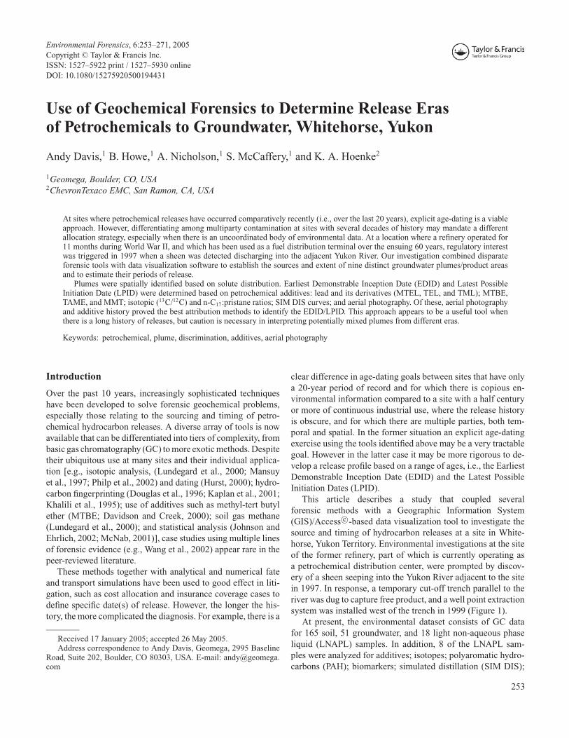
Environmental Forensics, 6:253–271, 2005Copyright C© Taylor & Francis Inc.ISSN: 1527–5922 print / 1527–5930 onlineDOI: 10.1080/15275920500194431

Use of Geochemical Forensics to Determine Release Erasof Petrochemicals to Groundwater, Whitehorse, Yukon

Andy Davis,1 B. Howe,1 A. Nicholson,1 S. McCaffery,1 and K. A. Hoenke2

1Geomega, Boulder, CO, USA2ChevronTexaco EMC, San Ramon, CA, USA

At sites where petrochemical releases have occurred comparatively recently (i.e., over the last 20 years), explicit age-dating is a viableapproach. However, differentiating among multiparty contamination at sites with several decades of history may mandate a differentallocation strategy, especially when there is an uncoordinated body of environmental data. At a location where a refinery operated for11 months during World War II, and which has been used as a fuel distribution terminal over the ensuing 60 years, regulatory interestwas triggered in 1997 when a sheen was detected discharging into the adjacent Yukon River. Our investigation combined disparateforensic tools with data visualization software to establish the sources and extent of nine distinct groundwater plumes/product areasand to estimate their periods of release.

Plumes were spatially identified based on solute distribution. Earliest Demonstrable Inception Date (EDID) and Latest PossibleInitiation Date (LPID) were determined based on petrochemical additives: lead and its derivatives (MTEL, TEL, and TML); MTBE,TAME, and MMT; isotopic (13C/12C) and n-C17:pristane ratios; SIM DIS curves; and aerial photography. Of these, aerial photographyand additive history proved the best attribution methods to identify the EDID/LPID. This approach appears to be a useful tool whenthere is a long history of releases, but caution is necessary in interpreting potentially mixed plumes from different eras.

Keywords: petrochemical, plume, discrimination, additives, aerial photography

Introduction

Over the past 10 years, increasingly sophisticated techniqueshave been developed to solve forensic geochemical problems,especially those relating to the sourcing and timing of petro-chemical hydrocarbon releases. A diverse array of tools is nowavailable that can be differentiated into tiers of complexity, frombasic gas chromatography (GC) to more exotic methods. Despitetheir ubiquitous use at many sites and their individual applica-tion [e.g., isotopic analysis, (Lundegard et al., 2000; Mansuyet al., 1997; Philp et al., 2002) and dating (Hurst, 2000); hydro-carbon fingerprinting (Douglas et al., 1996; Kaplan et al., 2001;Khalili et al., 1995); use of additives such as methyl-tert butylether (MTBE; Davidson and Creek, 2000); soil gas methane(Lundegard et al., 2000); and statistical analysis (Johnson andEhrlich, 2002; McNab, 2001)], case studies using multiple linesof forensic evidence (e.g., Wang et al., 2002) appear rare in thepeer-reviewed literature.

These methods together with analytical and numerical fateand transport simulations have been used to good effect in liti-gation, such as cost allocation and insurance coverage cases todefine specific date(s) of release. However, the longer the his-tory, the more complicated the diagnosis. For example, there is a

Received 17 January 2005; accepted 26 May 2005.Address correspondence to Andy Davis, Geomega, 2995 Baseline

Road, Suite 202, Boulder, CO 80303, USA. E-mail: [email protected]

clear difference in age-dating goals between sites that have onlya 20-year period of record and for which there is copious en-vironmental information compared to a site with a half centuryor more of continuous industrial use, where the release historyis obscure, and for which there are multiple parties, both tem-poral and spatial. In the former situation an explicit age-datingexercise using the tools identified above may be a very tractablegoal. However in the latter case it may be more rigorous to de-velop a release profile based on a range of ages, i.e., the EarliestDemonstrable Inception Date (EDID) and the Latest PossibleInitiation Dates (LPID).

This article describes a study that coupled severalforensic methods with a Geographic Information System(GIS)/Access c©-based data visualization tool to investigate thesource and timing of hydrocarbon releases at a site in White-horse, Yukon Territory. Environmental investigations at the siteof the former refinery, part of which is currently operating asa petrochemical distribution center, were prompted by discov-ery of a sheen seeping into the Yukon River adjacent to the sitein 1997. In response, a temporary cut-off trench parallel to theriver was dug to capture free product, and a well point extractionsystem was installed west of the trench in 1999 (Figure 1).

At present, the environmental dataset consists of GC datafor 165 soil, 51 groundwater, and 18 light non-aqueous phaseliquid (LNAPL) samples. In addition, 8 of the LNAPL sam-ples were analyzed for additives; isotopes; polyaromatic hydro-carbons (PAH); biomarkers; simulated distillation (SIM DIS);

253

254 A. Davis et al.

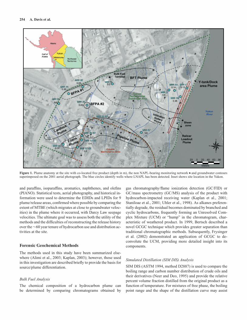
Figure 1. Plume anatomy at the site with co-located free product (depth in m), the non NAPL-bearing monitoring network and groundwater contourssuperimposed on the 2001 aerial photograph. The blue circles identify wells where LNAPL has been detected. Inset shows site location in the Yukon.

and paraffins, isoparaffins, aromatics, naphthenes, and olefins(PIANO). Statistical tests, aerial photography, and historical in-formation were used to determine the EDIDs and LPIDs for 9plume/release areas, confirmed where possible by comparing theextent of MTBE (which migrates at close to groundwater veloc-ities) in the plume where it occurred, with Darcy Law seepagevelocities. The ultimate goal was to assess both the utility of themethods and the difficulties of reconstructing the release historyover the ∼60 year tenure of hydrocarbon use and distribution ac-tivities at the site.

Forensic Geochemical Methods

The methods used in this study have been summarized else-where (Alimi et al., 2003; Kaplan, 2003); however, those usedin this investigation are described briefly to provide the basis forsource/plume differentiation.

Bulk Fuel Analysis

The chemical composition of a hydrocarbon plume canbe determined by comparing chromatograms obtained by

gas chromatography/flame ionization detection (GC/FID) orGC/mass spectrometry (GC/MS) analysis of the product withhydrocarbon-impacted receiving water (Kaplan et al., 2001;Staniloae et al., 2001; Uhler et al., 1998). As alkanes preferen-tially degrade, the residual becomes dominated by branched andcyclic hydrocarbons, frequently forming an Unresolved Com-plex Mixture (UCM) or “hump” in the chromatogram, char-acteristic of weathered product. In 1999, Bertsch described anovel GCGC technique which provides greater separation thantraditional chromatographic methods. Subsequently, Frysingeret al. (2002) demonstrated an application of GCGC to de-convolute the UCM, providing more detailed insight into itscomponents.

Simulated Distillation (SIM DIS) Analysis

SIM DIS (ASTM 1994, method D2887) is used to compare theboiling range and carbon number distribution of crude oils andtheir derivatives (Neer and Deo, 1995) and provide the relativepercent volume fraction distilled from the original product as afunction of temperature. For mixtures of free phase, the boilingpoint range and the shape of the distillation curve may assist

Release Eras of Petrochemicals to Groundwater 255

in determining the relative amounts of each fuel in the mixture(Kaplan et al., 1997).

Paraffins, Isoparaffins, Aromatics, Naphthenes, and Olefins(PIANO)

The PIANO analysis differentiates among fuel types based oncomposition over the C3 to C13 range (Kaplan et al., 1997).PIANO analyses are useful in distinguishing refined productsand the amount of ensuing degradation in the environment.These analyses also reflect evolving practices in gasoline pro-duction because the relative percentage of PIANO constituentshave changed over time in response to improvements in refining,the need to increase octane, and environmental regulations. Forexample, by the mid-1930s, thermal cracking produced gaso-lines with a lower olefin and higher octane-boosting aromaticcontent. In the 1950s olefins comprised 15–20%, decreasing to1% in 1974, before increasing to ∼10% from 1975 to the present.Aromatic content was approximately 12–14% by volume in the1950s, 20% in 1974, 32% in 1990, and is currently >40%.

Gasoline and Diesel Additives

The use of additives to date environmental organic residues hasbeen described thoroughly by Kaplan (2003). Briefly, lead (Pb)as tetraethyl lead (TEL) was added to gasoline as an antiknockagent beginning in 1923. In 1926, the maximum concentra-tion was regulated at 3.17 g Pb/gal of gasoline, increasing to4.23 g Pb/gal in 1959, but varying with individual refinery prac-tices (Gibbs, 1990). In 1978 the concentration was lowered to amaximum of 0.8 g Pb/gal for large refineries and 2.65 g Pb/galfor small refineries, and in 1983 lowered again to a pool limitof 1.1 g Pb/gal for all refineries. By July 1985, the average de-creased to 0.5 g Pb/gal, and then 0.1 g Pb/gal in 1988, main-tained until complete Pb phase-out (except in aviation gasoline)in 1995. A mixture of TEL, tetramethyl lead (TML), trimethylethyl lead (TMEL), dimethyl diethyl lead (DMDEL), and methyltriethyl lead (MTEL) was introduced in the 1960s (Hurst et al.,1996). After 1985, TEL remained the most widely used leadgasoline additive (Wakim et al., 1990). In Canada, Pb was phasedout in 1990 (Health Canada, 2004).

In the U.S., methylcyclopentadienyl manganese tricarbonyl(MMT) was added to gasoline as an antiknocking agent begin-ning in 1959, but used in conjunction with TEL only by smallrefineries until 1975, when MMT use began in both leaded andunleaded gasoline. By 1978, MMT could no longer be usedin unleaded gasoline in the U.S., until a 1995 EPA waiver al-lowed MMT in non-reformulated gasoline at 31 mg/gal. Absenceof MMT in gasoline does not necessarily indicate a post-1978gasoline because it was not added by all manufacturers (Hurstet al., 1996). In Canada, MMT use differed, in that it has beenadded continuously (up to 68 mg/gal) since 1977 (Health EffectsInstitute, 1998).

The addition of tert-butyl alcohol (TBA) and methyl tert-butyl ether (MTBE) to gasoline commenced in 1979 but thelatter was not widely used until 1987. Ethyl tertiary butyl ether

(ETBE) and tert amyl methyl ether (TAME) began appearingin gasoline in the early 1990s (Kaplan, 2003) although TAMEmay be an impurity (<0.2%) in MTBE (JRC, 2002). In Canada,MTBE use patterns have been similar to the U.S., being intro-duced in 1986 (Health Canada, 2003). However, while MTBEhas been phased out in the U.S., there is no current authority toban MTBE in Canada, although its use has been declining since1998 (Environment Canada, 2003).

Polyaromatic Hydrocarbons (PAHs)

Alykylated PAH homologues have differing degrees of resis-tance to weathering (Alimi et al., 2003), but their relativelongevity compared to monoaromatic ring compounds and alka-nes make them useful in distinguishing sources among heavierend hydrocarbons, and refined from unrefined products (Khaliliet al., 1995). This class of compounds has been used to sourcePAHs in sediment (Stout et al., 2001a) and to characterize dif-ferent petrogenic components of the Exxon Valdez spill (Wangand Fingas, 1995).

Biomarkers

Biomarkers are diagenetic alteration products of compoundsproduced by living organisms (Peters and Moldowan, 1993),that reflect different depositional (e.g., marine, lacustrine, fluvio-deltaic or hypersaline) environments and can be used to dis-tinguish different sources. Steranes and hopanes represent themost refractory biomarkers (Alimi et al., 2003), while two of themost commonly found and useful biomarkers are pristane andphytane—isoprenoid compounds formed from the phytol sidechain on the chlorophyll molecule (Tissot and Welte, 1984).

Dating Petrochemical Releases: Isotopes and Ratios

Estimating the age of diesel in groundwater has been proposedbased on the relative weathering rates of n-C17:pristane. Us-ing data from several diesel spills in Denmark released over arange of 20 years, Christensen and Larson (1993) developed therelationship:

T(year) = −8.4

(n − C17

Pr

)+ 19.8 (1)

where T is the age in years and n-C17 and Pr are the concentra-tions of the hydrocarbons. The average ratio in dispensed dieselfuel is 2.3, decreasing with weathering. Wade (2001) shows amethod accuracy of ±2 years when this method was appliedto product in Massachusetts soils. Recent expert opinion gener-ally considers the method applicable, with caveats (Alimi, 2002;Kaplan, 2002; Stout et al., 2002; Wade, 2002).

The ratios of 206Pb/207Pb in a mixture have also been used toidentify different lead sources based on the Anthropogenic LeadArchaeostratigraphy (ALAS) method of Hurst et al. (1996), whoused the changing Pb sources (and therefore, varying Pb isotoperatios) in gasoline from 1955–1995 to estimate release dates.

256 A. Davis et al.

Products from different source areas may also have differ-ent 13C/12C stable isotope ratios (Kaplan, 1997; Mansuy et al.,1997), potentially segregating plume elements from differentsources. The light isotope (12C) is preferentially volatilized bybiogenic processes over the heavy isotope (13C). Hence, differ-ent decomposition products have a different stable isotope dis-tribution. In addition, oxygen and carbon isotopic ratios can beused to monitor the pathways and rates of in situ biodegradation(Aggarwal et al., 1997).

Dating petrochemical releases has also been undertaken usingthe toluene:n-C8 ratio (Schmidt et al., 2002). As refining tech-niques improved between 1973 and 1992, the ratio increasedin a more or less uniform manner (from 0–10 ± 2.5) beforeincreasing sharply (to ∼20 ± 10) in 1995.

Statistical Analysis

Multivariate datasets are difficult to visualize, so techniques suchas Cluster Analysis and Principal Component Analysis are usedto reduce the number of variables displayed. Cluster Analysisis based on the “distance” between samples calculated from themeasurements of several parameters (Kaufman and Rousseeuw,1990). A variety of algorithms have been developed to formclusters of “closely spaced” samples that are based on minimiz-ing average distances within clusters and maximizing distancesbetween clusters. An alternative approach to forming distinctclusters is to use the distance values to form a “taxonomic tree”that shows the relationship among samples. This technique (hi-erarchical clustering) graphically displays the relative proximityof the samples in multidimensional parameter space.

Principal Components Analysis (PCA) groups the data intofactors, such that the first group contains most of the variabilityof the dataset, with subsequent components accounting for adecreasing fraction of the total variance (Johnson and Ehrlich,2002). Similar to Cluster Analysis, PCA provides a qualitativeanalysis of the importance of different variables. It has been usedin several environmental forensic investigations, for example, toallocate PAH in sediment to various sources (Burns et al., 1997),to correlate a heavy fuel oil spill to candidate ocean vessels (Stoutet al., 2001b), and to elucidate stressors to macrofauna exposedto sewage (Hopkins and Mudge, 2004).

Determining Release Source and Absolute Age

On aggregate, it appears that state-of-the-art forensicgeochemistry allows verifiable source identification usingchromatographic techniques, but exact age-dating in litigation,multi-party cost recovery, or in responding to insurance coverageclaims is more challenging as the period of record expands be-yond the 10- to 20-year period. Even under ideal circumstances,environmental conditions may render definitive age-dating (e.g.,to ±1 year) uncertain, and such estimates are often controversial.Therefore, as an adjunct, especially for application to older re-leases, we propose the use of a range of release periods, namelyan Earliest Demonstrable Inception Date (EDID), representing

the oldest demonstrable release age, and a Latest Possible Initi-ation Date (LPID), defining the most recent source release date.For long-term occupancy (LTO) sites even these constructs maylack specificity for mixed plumes, if the compounds used to de-termine the EDID (e.g., MMT) post-date an earlier release ofcommon constituents (e.g., benzene), or for the LPID if therewere ongoing releases of a compound (e.g., MTBE) subsequentto its first known use.

This approach provides additional insights to source-releasedynamics because despite the usefulness of exact age-datingtechniques, for example, the n-C17:pristane method (Christensenand Larsen, 1993), the B+T/E+X (Kaplan and Galperin, 1996)and n-C8:toluene (Schmidt et al., 2002) ratios, and lead isotopes(Hurst et al., 1996), all may be subject to ambiguity on an em-pirical basis due to site-specific differences in weathering ratescompared to the original demonstration (for the organic ratios),and/or the need to extrapolate from a standard curve to a localsite condition (for isotopic methods). Therefore, especially forLTO sites, the most robust approach to dating releases may be todetermine an age range, rather than an absolute date, by employ-ing multiple and disparate forensic tools to develop a weight-of-evidence approach to determine the vintage of a petrochemicalrelease.

Site History

Large-scale petrochemical use first occurred in 1944, follow-ing construction of the Canol Refinery in Whitehorse, Yukon, tosupport the Alaska-Canadian Highway. Construction of this roadwas initiated to bring wartime supplies into Alaska in prepara-tion for a potential invasion by Japan. The refinery operated for<1 year until it was decommissioned in April 1945, generating∼867,000 barrels of product derived from Norman Wells Crude(NWC) oil stock, piped directly from Norman Wells, NorthwestTerritories (Standard Oil, 1945).

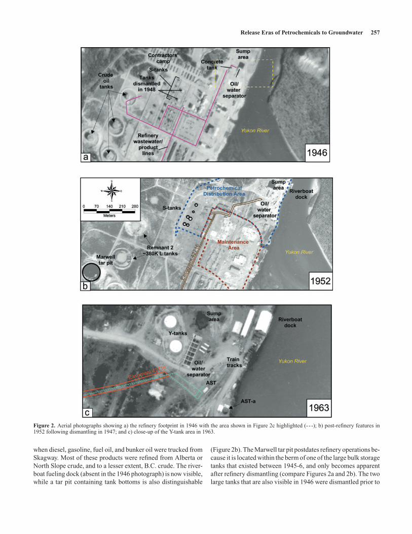
Prominent features include tanks, a contractors camp usedfor employee housing, an oil/water separator, and a wastew-ater/product line (Figure 2a). The oil/water separator, locatedin the northeastern portion of the site, was used to treat efflu-ent from the storm water sewer, incorporating washdown frombuilding floors, drains, equipment and spills (Midnight Arts,1999). Surface water runoff was collected in a sump prior totreatment in the separator and oil removed from the separatorwas sent to the slop tanks. The refinery was dismantled betweenthe fall of 1947 to late April of 1948 following the cessation ofwartime hostilities.

Within a year after refinery demolition, the site was in use forpetroleum storage and distribution operations and a portion forvehicle storage and highway maintenance activities (Figure 2b).The six Horton spheres (S-tanks) that were used during refin-ery operations were retained, and the oil/water separator andthe sump were also present in 1952. Gasoline was brought infirst by train, and then diesel and heating oil by pipeline fromSkagway. Later, finished products (gasoline and diesel) weresent through the Skagway pipeline until its retirement in 1996,


Figure 2. Aerial photographs showing a) the refinery footprint in 1946 with the area shown in Figure 2c highlighted (- - -); b) post-refinery features in1952 following dismantling in 1947; and c) close-up of the Y-tank area in 1963.

when diesel, gasoline, fuel oil, and bunker oil were trucked fromSkagway. Most of these products were refined from Alberta orNorth Slope crude, and to a lesser extent, B.C. crude. The river-boat fueling dock (absent in the 1946 photograph) is now visible,while a tar pit containing tank bottoms is also distinguishable

(Figure 2b). The Marwell tar pit postdates refinery operations be-cause it is located within the berm of one of the large bulk storagetanks that existed between 1945-6, and only becomes apparentafter refinery dismantling (compare Figures 2a and 2b). The twolarge tanks that are also visible in 1946 were dismantled prior to

258 A. Davis et al.

1952, since they are no longer visible in the 1952 aerial photo-graph (Figure 2b). The refinery pipelines were decommissionedupon closure; however, a pipeline was subsequently installed ineasement 42716 permitted across the site in 1960 (Figure 2b).

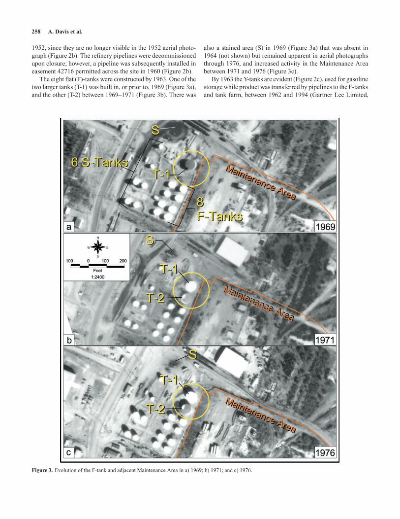
The eight flat (F)-tanks were constructed by 1963. One of thetwo larger tanks (T-1) was built in, or prior to, 1969 (Figure 3a),and the other (T-2) between 1969–1971 (Figure 3b). There was

Figure 3. Evolution of the F-tank and adjacent Maintenance Area in a) 1969; b) 1971; and c) 1976.

also a stained area (S) in 1969 (Figure 3a) that was absent in1964 (not shown) but remained apparent in aerial photographsthrough 1976, and increased activity in the Maintenance Areabetween 1971 and 1976 (Figure 3c).

By 1963 the Y-tanks are evident (Figure 2c), used for gasolinestorage while product was transferred by pipelines to the F-tanksand tank farm, between 1962 and 1994 (Gartner Lee Limited,


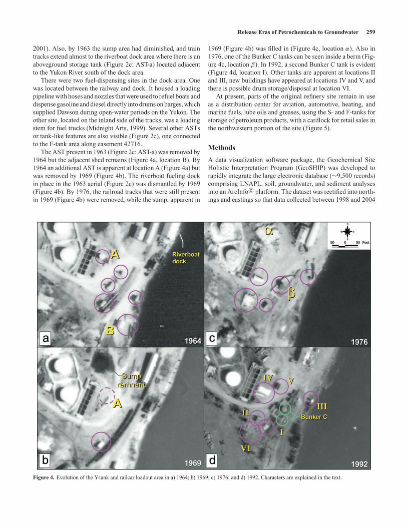
2001). Also, by 1963 the sump area had diminished, and traintracks extend almost to the riverboat dock area where there is anaboveground storage tank (Figure 2c: AST-a) located adjacentto the Yukon River south of the dock area.

There were two fuel-dispensing sites in the dock area. Onewas located between the railway and dock. It housed a loadingpipeline with hoses and nozzles that were used to refuel boats anddispense gasoline and diesel directly into drums on barges, whichsupplied Dawson during open-water periods on the Yukon. Theother site, located on the inland side of the tracks, was a loadingstem for fuel trucks (Midnight Arts, 1999). Several other ASTsor tank-like features are also visible (Figure 2c), one connectedto the F-tank area along easement 42716.

The AST present in 1963 (Figure 2c: AST-a) was removed by1964 but the adjacent shed remains (Figure 4a, location B). By1964 an additional AST is apparent at location A (Figure 4a) butwas removed by 1969 (Figure 4b). The riverboat fueling dockin place in the 1963 aerial (Figure 2c) was dismantled by 1969(Figure 4b). By 1976, the railroad tracks that were still presentin 1969 (Figure 4b) were removed, while the sump, apparent in

Figure 4. Evolution of the Y-tank and railcar loadout area in a) 1964; b) 1969; c) 1976; and d) 1992. Characters are explained in the text.

1969 (Figure 4b) was filled in (Figure 4c, location α). Also in1976, one of the Bunker C tanks can be seen inside a berm (Fig-ure 4c, location β). In 1992, a second Bunker C tank is evident(Figure 4d, location I). Other tanks are apparent at locations IIand III, new buildings have appeared at locations IV and V, andthere is possible drum storage/disposal at location VI.

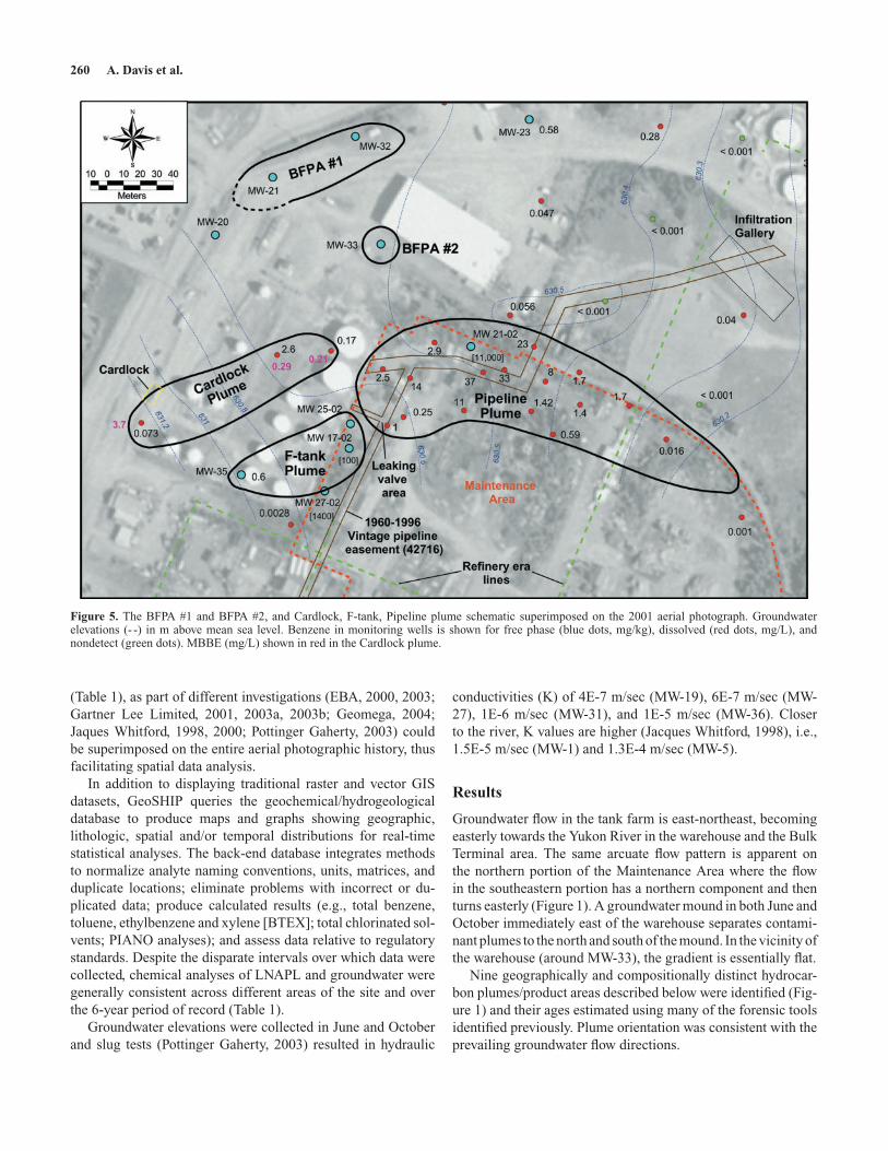
At present, parts of the original refinery site remain in useas a distribution center for aviation, automotive, heating, andmarine fuels, lube oils and greases, using the S- and F-tanks forstorage of petroleum products, with a cardlock for retail sales inthe northwestern portion of the site (Figure 5).

Methods

A data visualization software package, the Geochemical SiteHolistic Interpretation Program (GeoSHIP) was developed torapidly integrate the large electronic database (∼9,500 records)comprising LNAPL, soil, groundwater, and sediment analysesinto an ArcInfo c© platform. The dataset was rectified into north-ings and eastings so that data collected between 1998 and 2004

260 A. Davis et al.

Figure 5. The BFPA #1 and BFPA #2, and Cardlock, F-tank, Pipeline plume schematic superimposed on the 2001 aerial photograph. Groundwaterelevations (- -) in m above mean sea level. Benzene in monitoring wells is shown for free phase (blue dots, mg/kg), dissolved (red dots, mg/L), andnondetect (green dots). MBBE (mg/L) shown in red in the Cardlock plume.

(Table 1), as part of different investigations (EBA, 2000, 2003;Gartner Lee Limited, 2001, 2003a, 2003b; Geomega, 2004;Jaques Whitford, 1998, 2000; Pottinger Gaherty, 2003) couldbe superimposed on the entire aerial photographic history, thusfacilitating spatial data analysis.

In addition to displaying traditional raster and vector GISdatasets, GeoSHIP queries the geochemical/hydrogeologicaldatabase to produce maps and graphs showing geographic,lithologic, spatial and/or temporal distributions for real-timestatistical analyses. The back-end database integrates methodsto normalize analyte naming conventions, units, matrices, andduplicate locations; eliminate problems with incorrect or du-plicated data; produce calculated results (e.g., total benzene,toluene, ethylbenzene and xylene [BTEX]; total chlorinated sol-vents; PIANO analyses); and assess data relative to regulatorystandards. Despite the disparate intervals over which data werecollected, chemical analyses of LNAPL and groundwater weregenerally consistent across different areas of the site and overthe 6-year period of record (Table 1).

Groundwater elevations were collected in June and Octoberand slug tests (Pottinger Gaherty, 2003) resulted in hydraulic

conductivities (K) of 4E-7 m/sec (MW-19), 6E-7 m/sec (MW-27), 1E-6 m/sec (MW-31), and 1E-5 m/sec (MW-36). Closerto the river, K values are higher (Jacques Whitford, 1998), i.e.,1.5E-5 m/sec (MW-1) and 1.3E-4 m/sec (MW-5).

Results

Groundwater flow in the tank farm is east-northeast, becomingeasterly towards the Yukon River in the warehouse and the BulkTerminal area. The same arcuate flow pattern is apparent onthe northern portion of the Maintenance Area where the flowin the southeastern portion has a northern component and thenturns easterly (Figure 1). A groundwater mound in both June andOctober immediately east of the warehouse separates contami-nant plumes to the north and south of the mound. In the vicinity ofthe warehouse (around MW-33), the gradient is essentially flat.

Nine geographically and compositionally distinct hydrocar-bon plumes/product areas described below were identified (Fig-ure 1) and their ages estimated using many of the forensic toolsidentified previously. Plume orientation was consistent with theprevailing groundwater flow directions.


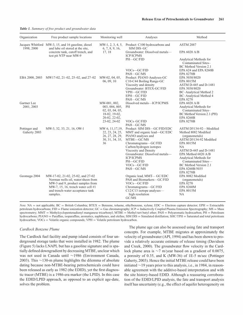
Table 1. Summary of free product and groundwater data

Organization Free product sample locations Monitoring well Analyses Method

Jacques Whitford1998, 2000

MW-3, 15, and 16 gasoline, dieseland lube oil stored at the site,concrete tank, cutoff trench, andtest pit NTP near MW-9

MW-1, 2, 3, 4, 5,6, 7, 8, 9, 16,17, 18

Product: C100 hydrocarbons andSIM DIS–GC

Groundwater: Dissolved metals—ICP/ICPMSPH—GC/FID

VOCs—GC/FIDPAH—GC/MS

ASTM 2887

EPA 6020 A/B

Analytical Methods forContaminated Sites–

BC Method Version 2.1EPA 624 and EPA 8260BEPA 8270B

EBA 2000, 2003 MW17-02, 21–02, 25–02, and 27–02 MW-02, 04, 05,06, 09, 10

Product: PIANO Analyses-GCC10-C44 Boiling Range-GCViscosity and densityGroundwater: BTEX-GC/FIDVPH—GC/FIDEPH—GC/FIDPAH—GC/MS

EPA 5030/8020EPA 8015MASTM D-445 and D-1481EPA 5030/8020BC–Analytical Method 2BC–Analytical Method 4EPA 8270

Gartner Lee2001, 2003

MW-001, 002,003, 004, 005,02, 03, 04, 05,18-02, 19-02,20-02, 22-02,23-02, 24-02

Dissolved metals—ICP/ICPMSPH

VOCs–GC/FIDPAH—GC/MS

EPA 6020 A/BAnalytical Methods for

Contaminated Sites–BC Method Version 2.1 (PH)EPA 8260BEPA 8270B

Pottinger andGaherty 2003

MW-3, 32, 33, 21, 16, OW-1 MW 6, 11,17,19,22, 23, 24, 25,26, 27, 28, 29,30, 31, 34, 35,36

Product: SIM DIS—GC/FID/EDCMMT and organic lead—GC/EDCPIANO analyses andMTBE—GC/MSChromatograms—GC/FIDCarbon/hydrogen isotopesViscosity and DensityGroundwater: Dissolved metals—ICP/ICPMSPH—GC/FIDVOCs—GC/FIDPAH—GC/MS

ASTM D5134-92—ModifiedMethod 8082 Modified

(organometals)ASTM D5134-92 ModifiedEPA 8015MNAASTM D-445 and D-1481EPA Method 6020 A/BAnalytical Methods for

Contaminated Sites—BC Method Version 2.1EPA 8260B/5035EPA 8270B

Geomega 2004 MW-17-02, 21-02, 25-02, and 27-02Norman wells oil, water/sheen fromMW-3 and 9, product samples fromMW-7, 15, 16, trench water cell #1and trench-water acceptance tanksamples.

Organic lead, MMT— GC/EDCPAH and Biomarkers—GC/FIDVOCs—GC/FIDChromatograms—GC/FIDC12/C13 isotope analyses—

high resolutionGC/MS

EPA 8082 Modified(organometals)

EPA 8270EPA 8260MEPA 8015MNA

Note. NA = not applicable; BC = British Columbia; BTEX = Benzene, toluene, ethylbenzene, xylene; EDC = Electron capture detector; EPH = Extractablepetroleum hydrocarbons; FID = Flame ionization detector; GC = Gas chromatography; ICP = Inductively Coupled Plasma Emission Spectrography; MS = Massspectrometry; MMT = Methylcyclopentenadienyl manganese tricarbonyl; MTBE = Methyl-tert butyl ether; PAH = Polyaromatic hydrocarbon; PH = Petroleumhydrocarbons; PIANO = Paraffins, isoparaffins, aromatics, naphthenes, and olefins; SIM DIS = Simulated distillation; SHC/TPH = Saturated and total petroleumhydrocarbon; VOCs = Volatile organic compounds; VPH = Volatile petroleum hydrocarbon.

Cardlock Benzene Plume

The Cardlock fuel facility and pump island consists of four un-derground storage tanks that were installed in 1982. The plume(Figure 5) lacks LNAPL but has a gasoline signature and is spa-tially defined downgradient by decreasing MTBE, unclear whichwas not used in Canada until ∼1986 (Environment Canada,2003). This ∼130-m plume highlights the dilemma of absolutedating because non-MTBE-bearing petrochemicals could havebeen released as early as 1982 (the EDID), yet the first diagnos-tic tracer (MTBE) is a 1986-era marker (the LPID). In this casethe EDID/LPID approach, as opposed to an explicit age-date,solves the problem.

The plume age can also be assessed using fate and transportconcepts. For example, MTBE migrates at approximately thevelocity of groundwater (API, 1994) and has been shown to pro-vide a relatively accurate estimate of release timing (Davidsonand Creek, 2000). The groundwater flow velocity in the Card-lock plume area is ∼7 m/year based on a gradient of 0.0075,a porosity of 0.35, and K (MW-36) of 1E-5 m/sec (PottingerGaherty, 2003). Hence the initial MTBE release could have beeninitiated ∼19 years prior to this analysis, i.e., in 1984, in reason-able agreement with the additive-based interpretation and withthe site history-based EDID. Although a reassuring corrobora-tion of the EDID/LPID analysis, the fate and transport analysisitself has uncertainty (e.g., the effect of aquifer heterogeneity on

262 A. Davis et al.

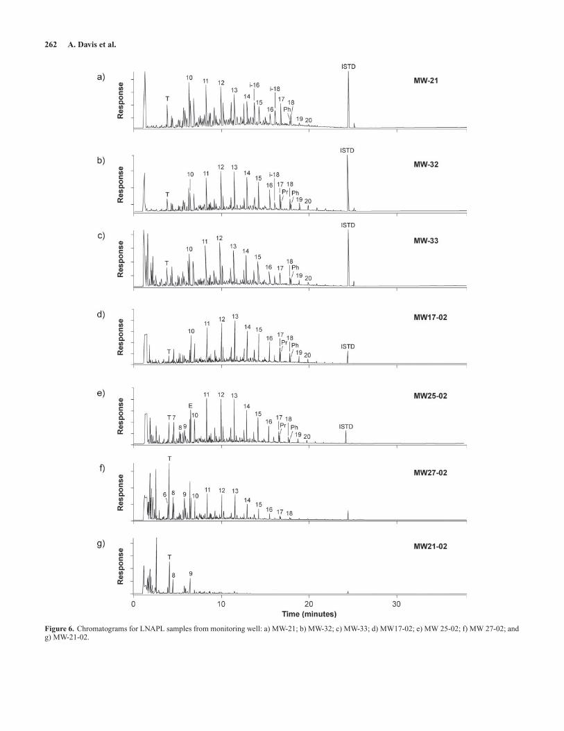
Figure 6. Chromatograms for LNAPL samples from monitoring well: a) MW-21; b) MW-32; c) MW-33; d) MW17-02; e) MW 25-02; f) MW 27-02; andg) MW-21-02.


K and the absolute extent of the MTBE plume). The variabilityassociated with such data could easily result in a release date of1984 ± 2 years.

Bulk Fuel Product Area (BFPA) #1 and #2

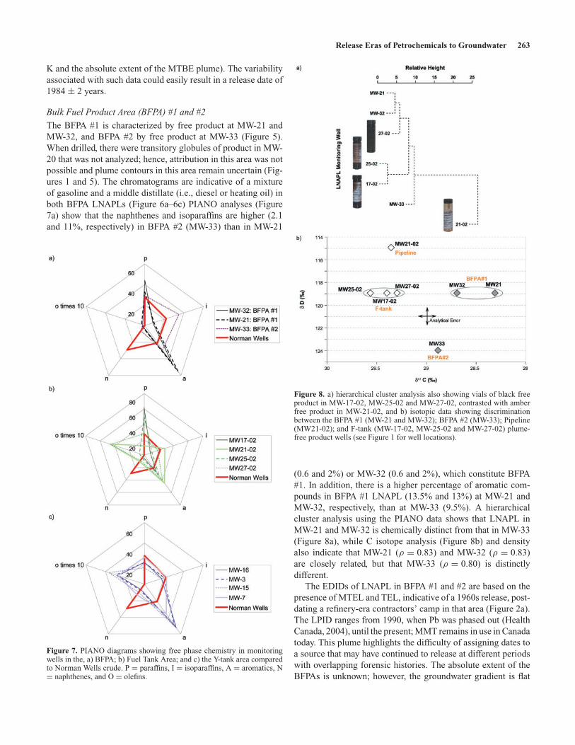
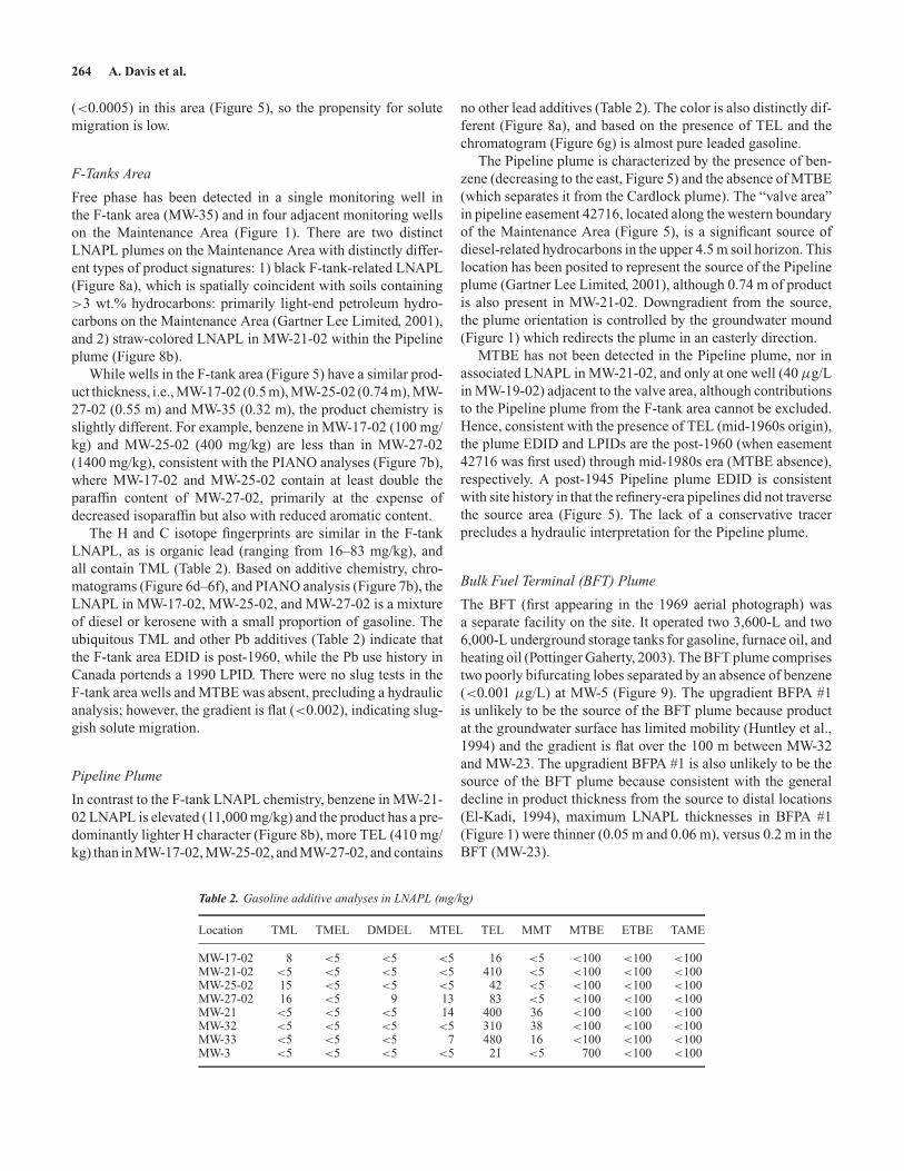
The BFPA #1 is characterized by free product at MW-21 andMW-32, and BFPA #2 by free product at MW-33 (Figure 5).When drilled, there were transitory globules of product in MW-20 that was not analyzed; hence, attribution in this area was notpossible and plume contours in this area remain uncertain (Fig-ures 1 and 5). The chromatograms are indicative of a mixtureof gasoline and a middle distillate (i.e., diesel or heating oil) inboth BFPA LNAPLs (Figure 6a–6c) PIANO analyses (Figure7a) show that the naphthenes and isoparaffins are higher (2.1and 11%, respectively) in BFPA #2 (MW-33) than in MW-21

Figure 7. PIANO diagrams showing free phase chemistry in monitoringwells in the, a) BFPA; b) Fuel Tank Area; and c) the Y-tank area comparedto Norman Wells crude. P = paraffins, I = isoparaffins, A = aromatics, N= naphthenes, and O = olefins.

Figure 8. a) hierarchical cluster analysis also showing vials of black freeproduct in MW-17-02, MW-25-02 and MW-27-02, contrasted with amberfree product in MW-21-02, and b) isotopic data showing discriminationbetween the BFPA #1 (MW-21 and MW-32); BFPA #2 (MW-33); Pipeline(MW21-02); and F-tank (MW-17-02, MW-25-02 and MW-27-02) plume-free product wells (see Figure 1 for well locations).

(0.6 and 2%) or MW-32 (0.6 and 2%), which constitute BFPA#1. In addition, there is a higher percentage of aromatic com-pounds in BFPA #1 LNAPL (13.5% and 13%) at MW-21 andMW-32, respectively, than at MW-33 (9.5%). A hierarchicalcluster analysis using the PIANO data shows that LNAPL inMW-21 and MW-32 is chemically distinct from that in MW-33(Figure 8a), while C isotope analysis (Figure 8b) and densityalso indicate that MW-21 (ρ = 0.83) and MW-32 (ρ = 0.83)are closely related, but that MW-33 (ρ = 0.80) is distinctlydifferent.

The EDIDs of LNAPL in BFPA #1 and #2 are based on thepresence of MTEL and TEL, indicative of a 1960s release, post-dating a refinery-era contractors’ camp in that area (Figure 2a).The LPID ranges from 1990, when Pb was phased out (HealthCanada, 2004), until the present; MMT remains in use in Canadatoday. This plume highlights the difficulty of assigning dates toa source that may have continued to release at different periodswith overlapping forensic histories. The absolute extent of theBFPAs is unknown; however, the groundwater gradient is flat

264 A. Davis et al.

(<0.0005) in this area (Figure 5), so the propensity for solutemigration is low.

F-Tanks Area

Free phase has been detected in a single monitoring well inthe F-tank area (MW-35) and in four adjacent monitoring wellson the Maintenance Area (Figure 1). There are two distinctLNAPL plumes on the Maintenance Area with distinctly differ-ent types of product signatures: 1) black F-tank-related LNAPL(Figure 8a), which is spatially coincident with soils containing>3 wt.% hydrocarbons: primarily light-end petroleum hydro-carbons on the Maintenance Area (Gartner Lee Limited, 2001),and 2) straw-colored LNAPL in MW-21-02 within the Pipelineplume (Figure 8b).

While wells in the F-tank area (Figure 5) have a similar prod-uct thickness, i.e., MW-17-02 (0.5 m), MW-25-02 (0.74 m), MW-27-02 (0.55 m) and MW-35 (0.32 m), the product chemistry isslightly different. For example, benzene in MW-17-02 (100 mg/kg) and MW-25-02 (400 mg/kg) are less than in MW-27-02(1400 mg/kg), consistent with the PIANO analyses (Figure 7b),where MW-17-02 and MW-25-02 contain at least double theparaffin content of MW-27-02, primarily at the expense ofdecreased isoparaffin but also with reduced aromatic content.

The H and C isotope fingerprints are similar in the F-tankLNAPL, as is organic lead (ranging from 16–83 mg/kg), andall contain TML (Table 2). Based on additive chemistry, chro-matograms (Figure 6d–6f), and PIANO analysis (Figure 7b), theLNAPL in MW-17-02, MW-25-02, and MW-27-02 is a mixtureof diesel or kerosene with a small proportion of gasoline. Theubiquitous TML and other Pb additives (Table 2) indicate thatthe F-tank area EDID is post-1960, while the Pb use history inCanada portends a 1990 LPID. There were no slug tests in theF-tank area wells and MTBE was absent, precluding a hydraulicanalysis; however, the gradient is flat (<0.002), indicating slug-gish solute migration.

Pipeline Plume

In contrast to the F-tank LNAPL chemistry, benzene in MW-21-02 LNAPL is elevated (11,000 mg/kg) and the product has a pre-dominantly lighter H character (Figure 8b), more TEL (410 mg/kg) than in MW-17-02, MW-25-02, and MW-27-02, and contains

Table 2. Gasoline additive analyses in LNAPL (mg/kg)

Location TML TMEL DMDEL MTEL TEL MMT MTBE ETBE TAME

MW-17-02 8 <5 <5 <5 16 <5 <100 <100 <100MW-21-02 <5 <5 <5 <5 410 <5 <100 <100 <100MW-25-02 15 <5 <5 <5 42 <5 <100 <100 <100MW-27-02 16 <5 9 13 83 <5 <100 <100 <100MW-21 <5 <5 <5 14 400 36 <100 <100 <100MW-32 <5 <5 <5 <5 310 38 <100 <100 <100MW-33 <5 <5 <5 7 480 16 <100 <100 <100MW-3 <5 <5 <5 <5 21 <5 700 <100 <100

no other lead additives (Table 2). The color is also distinctly dif-ferent (Figure 8a), and based on the presence of TEL and thechromatogram (Figure 6g) is almost pure leaded gasoline.

The Pipeline plume is characterized by the presence of ben-zene (decreasing to the east, Figure 5) and the absence of MTBE(which separates it from the Cardlock plume). The “valve area”in pipeline easement 42716, located along the western boundaryof the Maintenance Area (Figure 5), is a significant source ofdiesel-related hydrocarbons in the upper 4.5 m soil horizon. Thislocation has been posited to represent the source of the Pipelineplume (Gartner Lee Limited, 2001), although 0.74 m of productis also present in MW-21-02. Downgradient from the source,the plume orientation is controlled by the groundwater mound(Figure 1) which redirects the plume in an easterly direction.

MTBE has not been detected in the Pipeline plume, nor inassociated LNAPL in MW-21-02, and only at one well (40 μg/Lin MW-19-02) adjacent to the valve area, although contributionsto the Pipeline plume from the F-tank area cannot be excluded.Hence, consistent with the presence of TEL (mid-1960s origin),the plume EDID and LPIDs are the post-1960 (when easement42716 was first used) through mid-1980s era (MTBE absence),respectively. A post-1945 Pipeline plume EDID is consistentwith site history in that the refinery-era pipelines did not traversethe source area (Figure 5). The lack of a conservative tracerprecludes a hydraulic interpretation for the Pipeline plume.

Bulk Fuel Terminal (BFT) Plume

The BFT (first appearing in the 1969 aerial photograph) wasa separate facility on the site. It operated two 3,600-L and two6,000-L underground storage tanks for gasoline, furnace oil, andheating oil (Pottinger Gaherty, 2003). The BFT plume comprisestwo poorly bifurcating lobes separated by an absence of benzene(<0.001 μg/L) at MW-5 (Figure 9). The upgradient BFPA #1is unlikely to be the source of the BFT plume because productat the groundwater surface has limited mobility (Huntley et al.,1994) and the gradient is flat over the 100 m between MW-32and MW-23. The upgradient BFPA #1 is also unlikely to be thesource of the BFT plume because consistent with the generaldecline in product thickness from the source to distal locations(El-Kadi, 1994), maximum LNAPL thicknesses in BFPA #1(Figure 1) were thinner (0.05 m and 0.06 m), versus 0.2 m in theBFT (MW-23).


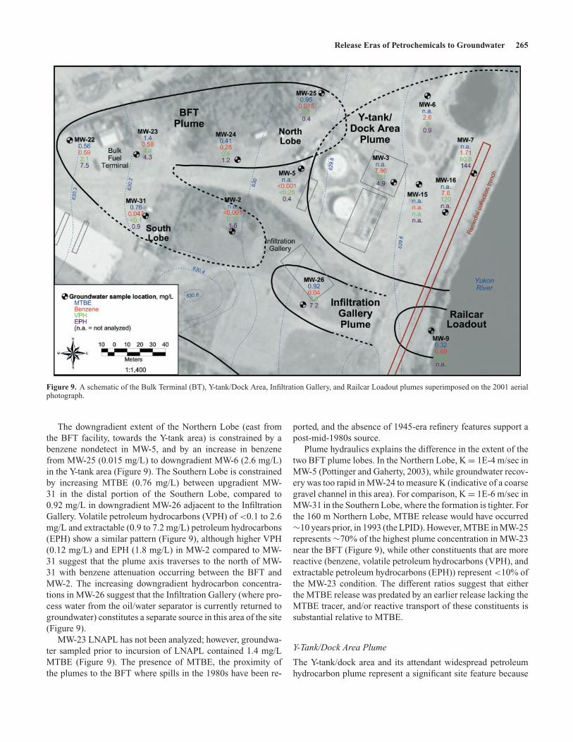
Figure 9. A schematic of the Bulk Terminal (BT), Y-tank/Dock Area, Infiltration Gallery, and Railcar Loadout plumes superimposed on the 2001 aerialphotograph.

The downgradient extent of the Northern Lobe (east fromthe BFT facility, towards the Y-tank area) is constrained by abenzene nondetect in MW-5, and by an increase in benzenefrom MW-25 (0.015 mg/L) to downgradient MW-6 (2.6 mg/L)in the Y-tank area (Figure 9). The Southern Lobe is constrainedby increasing MTBE (0.76 mg/L) between upgradient MW-31 in the distal portion of the Southern Lobe, compared to0.92 mg/L in downgradient MW-26 adjacent to the InfiltrationGallery. Volatile petroleum hydrocarbons (VPH) of <0.1 to 2.6mg/L and extractable (0.9 to 7.2 mg/L) petroleum hydrocarbons(EPH) show a similar pattern (Figure 9), although higher VPH(0.12 mg/L) and EPH (1.8 mg/L) in MW-2 compared to MW-31 suggest that the plume axis traverses to the north of MW-31 with benzene attenuation occurring between the BFT andMW-2. The increasing downgradient hydrocarbon concentra-tions in MW-26 suggest that the Infiltration Gallery (where pro-cess water from the oil/water separator is currently returned togroundwater) constitutes a separate source in this area of the site(Figure 9).

MW-23 LNAPL has not been analyzed; however, groundwa-ter sampled prior to incursion of LNAPL contained 1.4 mg/LMTBE (Figure 9). The presence of MTBE, the proximity ofthe plumes to the BFT where spills in the 1980s have been re-

ported, and the absence of 1945-era refinery features support apost-mid-1980s source.

Plume hydraulics explains the difference in the extent of thetwo BFT plume lobes. In the Northern Lobe, K = 1E-4 m/sec inMW-5 (Pottinger and Gaherty, 2003), while groundwater recov-ery was too rapid in MW-24 to measure K (indicative of a coarsegravel channel in this area). For comparison, K = 1E-6 m/sec inMW-31 in the Southern Lobe, where the formation is tighter. Forthe 160 m Northern Lobe, MTBE release would have occurred∼10 years prior, in 1993 (the LPID). However, MTBE in MW-25represents ∼70% of the highest plume concentration in MW-23near the BFT (Figure 9), while other constituents that are morereactive (benzene, volatile petroleum hydrocarbons (VPH), andextractable petroleum hydrocarbons (EPH)) represent <10% ofthe MW-23 condition. The different ratios suggest that eitherthe MTBE release was predated by an earlier release lacking theMTBE tracer, and/or reactive transport of these constituents issubstantial relative to MTBE.

Y-Tank/Dock Area Plume

The Y-tank/dock area and its attendant widespread petroleumhydrocarbon plume represent a significant site feature because

266 A. Davis et al.

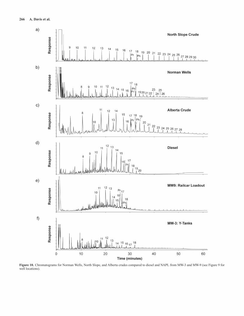
Figure 10. Chromatograms for Norman Wells, North Slope, and Alberta crudes compared to diesel and NAPL from MW-3 and MW-9 (see Figure 9 forwell locations).


of its proximity to the location (Figure 1) of the 1997 Yukon Riversheen observation, which initiated the original regulatory action.The Y-tank plume (Figure 9) extends from just north and west ofthe Y-tanks to the Yukon River and is separate from the RailcarLoadout plume in the same general area because the productin MW-9 has a predominantly diesel signature compared to theY-tank area signature, e.g., MW-3 (Figure 10f). A combination ofheavy residual compounds and diesel is not unexpected, becausedue to their viscosity, heating oil, Bunker C, and lubricatingoils are diluted with diesel in cold climates to improve theirflow characteristics (Kaplan, 2003). Bunker C and heating oil isknown to have been used in the Y-tank area.

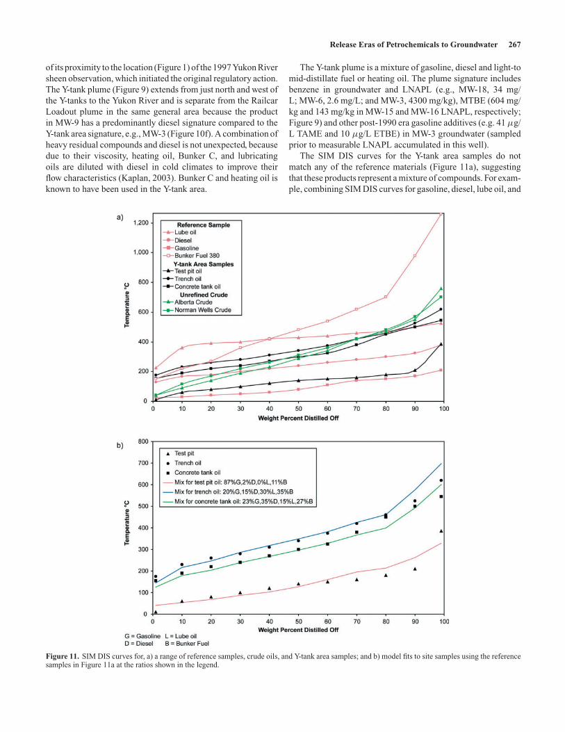
Figure 11. SIM DIS curves for, a) a range of reference samples, crude oils, and Y-tank area samples; and b) model fits to site samples using the referencesamples in Figure 11a at the ratios shown in the legend.

The Y-tank plume is a mixture of gasoline, diesel and light-tomid-distillate fuel or heating oil. The plume signature includesbenzene in groundwater and LNAPL (e.g., MW-18, 34 mg/L; MW-6, 2.6 mg/L; and MW-3, 4300 mg/kg), MTBE (604 mg/kg and 143 mg/kg in MW-15 and MW-16 LNAPL, respectively;Figure 9) and other post-1990 era gasoline additives (e.g. 41 μg/L TAME and 10 μg/L ETBE) in MW-3 groundwater (sampledprior to measurable LNAPL accumulated in this well).

The SIM DIS curves for the Y-tank area samples do notmatch any of the reference materials (Figure 11a), suggestingthat these products represent a mixture of compounds. For exam-ple, combining SIM DIS curves for gasoline, diesel, lube oil, and

268 A. Davis et al.

International Bunker Fuel (IBF) 380 in various ratios allows op-timization of mixtures to identify potential contributors to thetrench, test pit, and concrete tank oils. If gasoline (G), diesel(D), lube oil (L), and bunker fuel (B) represent the simulateddistillation data for gasoline, diesel, lube oil, and IBF 380, re-spectively (Figure 11a), and g, d, l, and b the percentage of thesimulated distillation data for gasoline, diesel, lube oil, and IBF380, respectively, then an estimate of the simulated distillationdata, X, for the test pit, trench, and concrete tank oils can beobtained from:

X = gG

100+ dD

100+ lL

100+ bB

100(2)

This equation was used to optimize mix ratios for all the sam-ples. For the trench and concrete tank oils in particular, there is

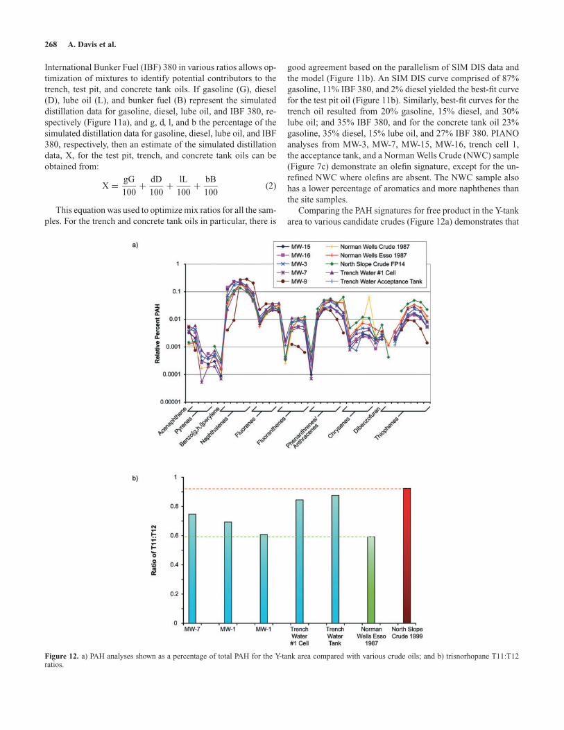
Figure 12. a) PAH analyses shown as a percentage of total PAH for the Y-tank area compared with various crude oils; and b) trisnorhopane T11:T12ratios.

good agreement based on the parallelism of SIM DIS data andthe model (Figure 11b). An SIM DIS curve comprised of 87%gasoline, 11% IBF 380, and 2% diesel yielded the best-fit curvefor the test pit oil (Figure 11b). Similarly, best-fit curves for thetrench oil resulted from 20% gasoline, 15% diesel, and 30%lube oil; and 35% IBF 380, and for the concrete tank oil 23%gasoline, 35% diesel, 15% lube oil, and 27% IBF 380. PIANOanalyses from MW-3, MW-7, MW-15, MW-16, trench cell 1,the acceptance tank, and a Norman Wells Crude (NWC) sample(Figure 7c) demonstrate an olefin signature, except for the un-refined NWC where olefins are absent. The NWC sample alsohas a lower percentage of aromatics and more naphthenes thanthe site samples.

Comparing the PAH signatures for free product in the Y-tankarea to various candidate crudes (Figure 12a) demonstrates that


product PAH profiles from MW-7, MW-15, MW-16, and trenchwater #1 cell are all very similar to North Slope, EdmontonSweet, and NWC (2 samples). Groundwater samples MW-3 andMW-9 have lower PAH concentrations but also show a similarPAH distribution to the crude oils. Even after plotting the dataon a relative scale (e.g., with concentrations reported as a frac-tion of �PAH) the signatures are too similar to unambiguouslydistinguish a crude oil source at this site.

Finally, biomarker analyses also exemplify the difficulty in-herent in attempting to identify free product sources in the Y-tankarea. For example, although the trinorhopane T11:T12 (T ratio)in MW-16 is similar to NWC, the #1 cell and the acceptancetank are similar to North Slope crude, while MW-7 and MW-15are intermediate between these end members (Figure 12b).

The n-C17:pristane age estimates for LNAPL in MW-7, MW-15, MW-16, and a trench water acceptance tank sample resultin a 14–19 years b.p. age range, in qualitative agreement withthe presence of MTBE, TAME, and ETBE (which also indicate∼10–15 year b.p. release). However, the toluene:n-C8 ratio (3.1in MW-15 and 4.5 in MW-16) is ambiguous, returning a releaseage of pre-1982. In summary, the EDID is post-1948 (basedon historical usage patterns), with an LPID of the early 1990sdue to the presence of TAME. Although they contain MTBE,neither the Y-tanks nor the Railcar Loadout plume lend them-selves to hydraulic release estimates because both are capturedby the well point system (Figure 1), and therefore have no finitedowngradient boundary.

Railcar Loadout Plume

The Railcar Loadout plume is co-located with the 1963AST/railcar offloading area in the vicinity of the seep discov-ered in 1997 (Figure 1). The sole monitoring well (MW-9) inthe Railcar Loadout plume lacks free product, although sheenhas been noted. MTBE (0.3 mg/L) and the MW-9 chromato-graph (Figure 10e) indicate that the contamination in this wellis predominantly diesel with a minor gasoline component.

Aviation gas with high Pb (1400–1500 mg/kg) was also han-dled at the Railcar Loadout and Pb (1343 mg/kg) was foundat a test pit in this area (Jacques Whitford, 2000), suggesting,in conjunction with historical use patterns (Figure 4), that thesheen may have been due to operations at the Railcar Loadoutarea. Since the Railcar Loadout is first recognizable on the 1963

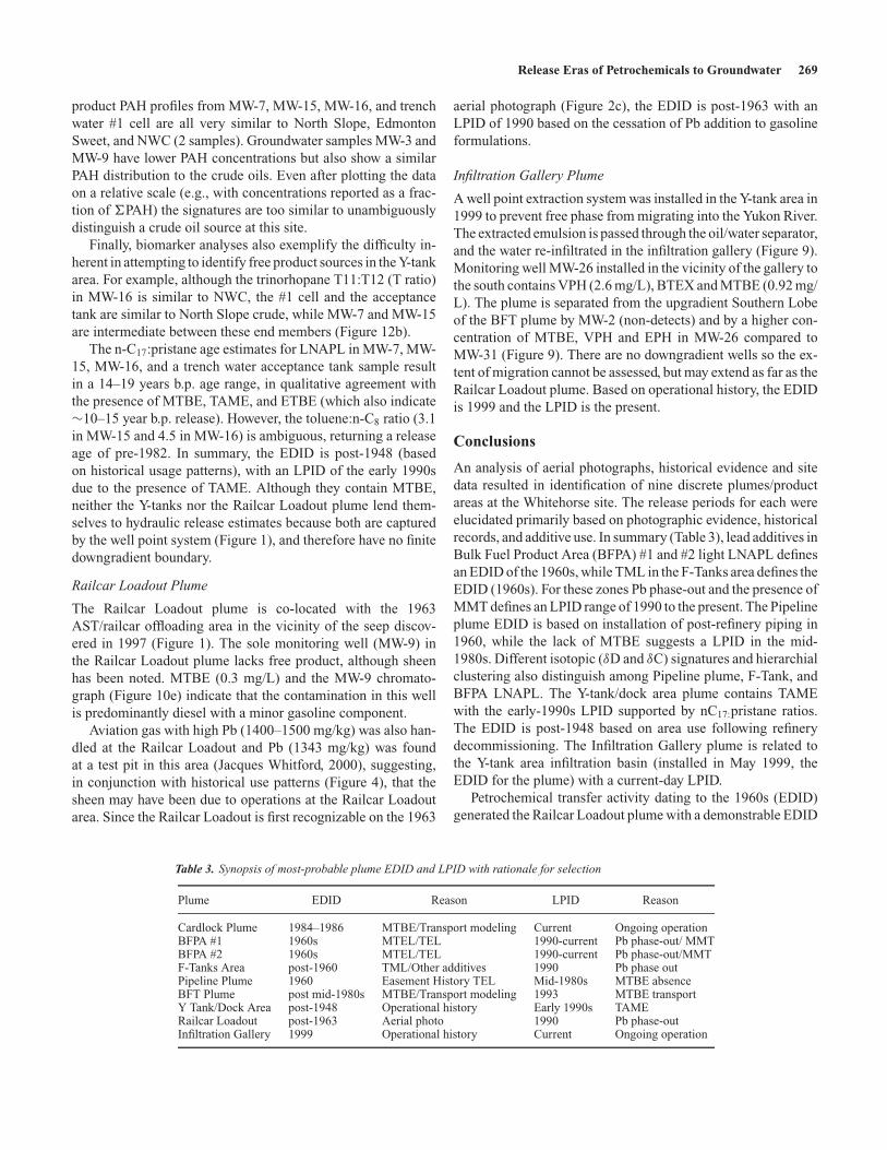
Table 3. Synopsis of most-probable plume EDID and LPID with rationale for selection

Plume EDID Reason LPID Reason

Cardlock Plume 1984–1986 MTBE/Transport modeling Current Ongoing operationBFPA #1 1960s MTEL/TEL 1990-current Pb phase-out/ MMTBFPA #2 1960s MTEL/TEL 1990-current Pb phase-out/MMTF-Tanks Area post-1960 TML/Other additives 1990 Pb phase outPipeline Plume 1960 Easement History TEL Mid-1980s MTBE absenceBFT Plume post mid-1980s MTBE/Transport modeling 1993 MTBE transportY Tank/Dock Area post-1948 Operational history Early 1990s TAMERailcar Loadout post-1963 Aerial photo 1990 Pb phase-outInfiltration Gallery 1999 Operational history Current Ongoing operation

aerial photograph (Figure 2c), the EDID is post-1963 with anLPID of 1990 based on the cessation of Pb addition to gasolineformulations.

Infiltration Gallery Plume

A well point extraction system was installed in the Y-tank area in1999 to prevent free phase from migrating into the Yukon River.The extracted emulsion is passed through the oil/water separator,and the water re-infiltrated in the infiltration gallery (Figure 9).Monitoring well MW-26 installed in the vicinity of the gallery tothe south contains VPH (2.6 mg/L), BTEX and MTBE (0.92 mg/L). The plume is separated from the upgradient Southern Lobeof the BFT plume by MW-2 (non-detects) and by a higher con-centration of MTBE, VPH and EPH in MW-26 compared toMW-31 (Figure 9). There are no downgradient wells so the ex-tent of migration cannot be assessed, but may extend as far as theRailcar Loadout plume. Based on operational history, the EDIDis 1999 and the LPID is the present.

Conclusions

An analysis of aerial photographs, historical evidence and sitedata resulted in identification of nine discrete plumes/productareas at the Whitehorse site. The release periods for each wereelucidated primarily based on photographic evidence, historicalrecords, and additive use. In summary (Table 3), lead additives inBulk Fuel Product Area (BFPA) #1 and #2 light LNAPL definesan EDID of the 1960s, while TML in the F-Tanks area defines theEDID (1960s). For these zones Pb phase-out and the presence ofMMT defines an LPID range of 1990 to the present. The Pipelineplume EDID is based on installation of post-refinery piping in1960, while the lack of MTBE suggests a LPID in the mid-1980s. Different isotopic (δD and δC) signatures and hierarchialclustering also distinguish among Pipeline plume, F-Tank, andBFPA LNAPL. The Y-tank/dock area plume contains TAMEwith the early-1990s LPID supported by nC17:pristane ratios.The EDID is post-1948 based on area use following refinerydecommissioning. The Infiltration Gallery plume is related tothe Y-tank area infiltration basin (installed in May 1999, theEDID for the plume) with a current-day LPID.

Petrochemical transfer activity dating to the 1960s (EDID)generated the Railcar Loadout plume with a demonstrable EDID

270 A. Davis et al.

of 1963 and an LPID of 1990 based on Pb phase-out. Spill historyinfers initiation of the BFT plume by the mid-1980s while MTBEtransport defines a LPID of 1993. The Cardlock plume is alsoof recent vintage, with an EDID in the mid-1980s based on theMTBE signature and with a present-day LPID because this areais in an active part of the facility.

On aggregate, this investigation demonstrates the utility ofmultiple forensic techniques in determining an age range forpetrochemical releases where defining a specific age may bemore tenuous. However, it is important to understand constraintson the accuracy of exact dating of releases at complex LTOsites where a range of release dates may be a more tractablegoal. For each plume at Whitehorse the EDID was defined, al-though in cases where there is no corroborating information,the initiation time could be earlier if there were superimpositionof later releases which contained a dating tracer on earlier re-leases of common constituents which lacked the tracer (i.e., amixed plume), or if the EDID is based solely on photographicinterpretation.

The LPID provides the most recent potential starting datefor the source, with the understanding that introduction of ad-ditives to Canadian petrochemical products may have followeda slightly later trajectory than for their U.S. counterparts, pos-sibly resulting in a more recent LPID. Finally, ongoing releasesare transparent to the LPID because a release of petrochemicalsbearing the LPID tracer could continue after the LPID.

This case study also provides some useful insights into thelevel of confidence that can be placed on various forensic toolsin field applications. Clearly, in this case the GC analytical andadditives data were diagnostic in identifying classes of petro-chemicals released to the environment, while the extensive aerialphotographic record and historical information provide bound-ing dates based on the presence and evolving nature of the fa-cility. The isotopic and SIM DIS data provided discriminatorysupport in separating LNAPL types, but not independent evi-dence to date releases, while the PAH and biomarker data wereambiguous. Finally, age-dating using n-C17:pristane providessubjective support for some of the conclusions, while whereMTBE is present, a transport analysis provides useful corrobo-rative information that is internally consistent with the knownsite history and plume dimensions.

Acknowledgements

We appreciate the constructive and thought-provoking com-ments of three anonymous reviewers who helped improve anearlier version of the manuscript.

References

Aggarwal, P. K., Fuller, M. E., Gurgas, M. M., Manning, J. F., and Dillon,M. A. 1997. Use of stable oxygen and carbon isotope analyses for monitor-ing the pathways and rates of intrinsic and enhanced in situ biodegradation.Environ. Sci. Technol. 31:590–596.

Alimi, H. 2002. Invited commentary on the Christensen and Larsen tech-nique. Environ. Forensics 3:5.

Alimi, H., Ertel, T., and Schug, B. 2003. Fingerprinting of hydrocar-bon fuel contaminants: Literature review. Environmental Forensics 4:25–38.

API (American Petroleum Institute). 1994. Transport and fate of dissolvedmethanol, methyl-tertiary-butyl-ether, and monoaromatic hydrocarbonsin a shallow sand aquifer. Washington, DC. API Publication 4601.

ASTM (American Society for Testing and Materials). 1994. Annual bookof ASTM standards. Philadelphia, PA. Vol. 02.04

Bertsch, W. 1999. Two-dimensional gas chromatography. Concepts, in-strumentation, and applications-Part 1: fundamentals, conventional two-dimensional gas chromatography, selected applications. J. High Resol.Chromatogr. 22:647–665.

Burns, W. A., Mankiewicz, P. J., Bence, A. E., Page, D. S., and Parker,K. R. 1997. A principal component and least squares method for allo-cating polycyclic aromatic hydrocarbons in sediment to multiple sources.Environ. Toxicol. Chem. 16:1119–1131.

Christensen, L. B., and Larsen, T. H. 1993. Method for determining the ageof diesel oil spills in the soil. Ground Water Monitoring and Remediation32(4):142–149.

Davidson, J. M., and Creek, D. N. 2000. Using the gasoline additive MTBEin forensic environmental investigations. Environmental Forensics 1:31–36.

Douglas, G. S., Bence, A. E., Prince, R. C., McMillan, S. J., and Butler,E. L. 1996. Environmental stability of selected petroleum hydrocarbonsource and weathering ratios. Environ. Sci. Technol. 30:2232–2239.

EBA Engineering Consultants Limited. 2000. Phase 1 & 2 environmentalsite assessment. Whitehorse Grader Station. Prepared for the Governmentof Yukon, Property Management Agency, EBA Engineering ConsultantsLimited, Whitehorse, Yukon, Canada.

EBA Engineering Consultants Limited. 2003. Product characterization atWhitehorse Grader Station. Prepared for Highways and Public Works,Government of Yukon. EBA Engineering Consultants Limited, White-horse, Yukon, Canada.

El-Kadi, A. I. 1994. Applicability of sharp-interface models for NAPLtransport: 2. spreading of a LNAPL. Ground Water 32:784–793.

Environment Canada. 2003. Use and release of MTBE in Canada. Oil,Gas and Energy Branch Environment Canada, March 2003. Available atwww.calgasoline.com/Cnmtbe0303.pdf

Frysinger, G. S., Gaines, R. B., and Reddy, C. M. 2002. GC × GC: Anew analytical tool for environmental forensics. Environ. Forensics 3:27–34.

Gartner Lee Limited. 2001. Whitehorse Grader Station Phase III environ-mental site assessment. Prepared for Government of Yukon, Community& Transportation Services. Whitehorse, Yukon.

Gartner Lee Limited. 2003a. Marwell Drainage Ditch construction: Envi-ronmental soil sampling program and related environmental works. Pre-pared for City of Whitehorse Engineering and Environmental Services.Whitehorse, Yukon.

Gartner Lee Limited. 2003b. Whitehorse Grader Station 2002 environmen-tal site assessment. Prepared for Highways and Public Works Lands andGranular Resources Branch Golder Associates Ltd. 1994. Yukon, BC andAlaska; Environmental Site Assessments. Whitehorse, Yukon.

Geomega. 2004. Characterization and forensic evaluation of hydrocarboncontamination at the former Canol Refinery Site Whitehorse, Yukon Ter-ritory. Geomega, Boulder, Co.

Gibbs, L. M. 1990. Gasoline additives: When and why. SAE Tech. Paper#902104. Int’l. Fuels and Lubricants Meeting, Oct. 1990. Soc. AutomotiveEng., Warrendale, PA.

Health Canada. 2004. Lead information package. Available at http://www.hc-sc.gc.ca / hecs-sesc / toxics management / publications / leadQandA/sources.htm#4

Health Effects Institute. 1998. Summary of a workshop on metal-based fueladditives and new engine technologies. February 4th. Bosto: Author.

Hopkins, F. E., and Mudge, S. M. 2004. Detecting anthropogenic stress in anecosystem: 2. Macrofauna in a sewage gradient. Environmental Forensics.5:213–224.

Huntley, D., Hawk, R. N., and Corley, H. P. 1994. Nonaqueous phase hy-drocarbon in a fine-grained sandstone: 1. comparison between measuredand predicted saturations and mobility. Ground Water. 32:626–634.


Hurst, R. W. 2000. Applications of anthropogenic lead archaeostratigraphyto (ALAS model) to hydrocarbon remediation. Environmental Forensics1:11–23.

Hurst, R. W., Davis, T. E., and Chinn, B. D. 1996. The lead fin-gerprints of gasoline contamination. Environ. Sci. Technol. 30:304A–307A.

Jacques Whitford Environment Limited. 1998. Site characterization andremediation assessment former Whitehorse Refinery. Whitehorse, YukonProject Number C6190.

Jacques Whitford Environment Limited. 2000. Supplemental Phase II en-vironmental site assessment former Whitehorse Refinery, Yukon.

Johnson, G. W., and Ehrlich, R. 2002. State of the art report on multivari-ate chemometric methods in environmental forensics. Environ. Forensics3:59–79.

JRC. (Joint Research Council). 2002. Tert-butyl methyl ether. Summary riskassessment report. European Commission Joint Research Council specialpublication 1.02.101., Ispra, Italy.

Kaplan, I. R. 2002. Invited commentary on the Christensen and Larsentechnique. Environ. Forensics 3:7.

Kaplan, I. R. 2003. Age dating of environmental organic residues. Environ-mental Forensics 4:95–141.

Kaplan, I. R., and Galperin, Y. 1996. How to recognize a hydrocarbon fuelin the environment and estimate its age of release. In Groundwater andsoil contamination: Technical preparation and litigation management, ed.T. J. Bois and B. J. Luther, 145–199. New York: Wiley Law Publishers.

Kaplan, I. R., Galperin, Y., Lu, S.-T., and Lee, R.-P. 1997. Forensic envi-ronmental geochemistry: Differentiation of fuel-types, their sources andrelease time. Organic Geochemistry 27:289–317.

Kaplan, I. R., Lu, S.-T., Alimi, H. M., and MacMurphey, J. 2001. Fin-gerprinting of high boiling hydrocarbons fuels, asphalts and lubricants.Environ. Forensics 2:231–248.

Kaufman, L., and Rousseeuw, P. J. 1990. Finding groups in data: An intro-duction to cluster analysis. New York: Wiley.

Khalili, N. R., Scheff, P. A., and Holsen, T. M. 1995. PAH source fingerprintsfor coke ovens, diesel and gasoline engines, highway tunnels, and woodcombustion emissions. Atm. Environ. 29:533–542.

Lundegard, P. D., Sweeney, R. E., and Ririe, G. T. 2000. Soil gas methaneat petroleum contaminated sites: forensic determination of origin andsource. Environ. Forensics 1:3–10.

Mansuy, L., Philp, R. P., and Allen, J. 1997. Source identification of oil spillsbased on the isotopic composition of individual components in weatheredoil samples. Environ. Sci. Technol. 31:3417–3425.

McNab, W. 2001. Forensic analysis of chlorinated hydrocarbon plumesin groundwater: A multi-site perspective. Environ. Forensics 2:313–320.

Midnight Arts. 1999. Marwell industrial area. Historical research project.Prepared for the Department of Renewable Resources, Government ofYukon and the City of Whitehorse.

Neer, L. A., and Deo, M. D. 1995. Simulated distillation of oils with awide carbon number distribution. Journal of Chromatographic Science3:133–138.

Peters, K. E., and Moldowan, J. M. 1993. The biomarker guide. EnglewoodCliffs, NJ: Prentice Hall.

Philp, R. P., Allen, J., and Kuder, T. 2002. The use of the isotopic compositionof individual compounds for correlating spilled oils and refined productsin the environment with suspected sources. Environ. Forensics 3:341–348.

Pottinger Gaherty. 2003. Environmental site investigation 146 IndustrialRoad, Whitehorse, Yukon. Vancouver, BC: Author.

Schmidt, G. W., Beckmann, D. D., and Torkelson, B. E. 2002. A techniquefor estimating the age of regular/mid-grade gasoline released to the sub-surface since the early 1970s. Environ. Forensics 3:145–162.

Standard Oil Company of California and Standard Oil Company (Alaska).1945. Completion Report. Operation of Norman Wells–Whitehorse PipeLine and Whitehorse Refinery. Under Contract No. W-2385-ENG-39.

Staniloae, D., Petrescu, B., and Patroescu, C. 2001. Pattern recognitionbased software for oil spills identification by gas chromatography and IRspectrophotometry. Environ. Forensics 2:363–366.

Stout, S. A., Magar, V. S., Uhler, R. M., Ickes, J., Abbott, J., and Brenner, R.2001a. Characterization of naturally-occurring and anthropogenic PAHsin urban sediments-Wycoff/Eagle harbor superfund site. Environ. Foren-sics 2:287–300.

Stout, S. A., Uhler, A. D., and McCarthy, K. J. 2001. A strategy and method-ology for defensibly correlating spilled oil to source candidates. Environ.Forensics 2:87–98.

Stout, S. A., Uhler, A. D., McCarthy, K. J., and Emsbo-Mattingly, S. D. 2002.Invited commentary on the Christensen and Larsen technique. Environ.Forensics 3:9–11.

Tissot, B. P., and Welte, D. H. 1984. Petroleum formation and occurrence(2nd rev. ed). Berlin: Springer Verlag.

Uhler, A. D., McCarthy, K. J., and Stout, S. A. 1998. Get to know yourpetroleum types. Soil and Groundwater Cleanup, July: xx.

Wade, M. J. 2001. Age-dating diesel fuel spills: Using the European em-pirical time-based model in the U.S.A. Environmental Forensics 2:347–358.

Wade, M. J. 2002. Invited commentary on the Christensen and Larsen tech-nique. Environ. Forensics 3:13.

Wakim, J. M., Schwendener, H., and Shimosato, J. 1990. Chemical eco-nomics handbook. Publication 543.75011. SRI International, Palo Alto,CA.

Wang, Z. D., and Fingas, M. 1995. Use of methyldibenzenethiophenes asmarkers for differentiation and source identification of crude and weath-ered oils. Environ. Sci. Technol. 29:2842–2849.

Wang, Z. D., Fingas, M., and Sigoouin, L. 2002. Using multiple criteria forfingerprinting unknown oil samples having very similar chemical com-position. Environ. Forensics 3:251–262.

Documents

Use of Geochemical Forensics to Determine Release Eras of Petrochemicals to Groundwater, Whitehorse, Yukon