Using VLBI fringe-phase information from geodetic experiments for short-period ionospheric studies

Journal of Geodesy manuscript No.(will be inserted by the editor)

Thomas Hobiger · Tetsuro Kondo · Yasuhiro

Koyama · Kazuhiro Takashima · Harald Schuh

Using VLBI fringe-phase information from geodetic

experiments for short-period ionospheric studies

Received: 09/05/2006 / Accepted: 05/02/2007

T. Hobiger

Kashima Space Research Center

National Institute of Information and Communications Technology (NICT)

893-1 Hirai, Kashima, 314-0012 Ibaraki, Japan

Tel.: +81-0-299-84-7136

Fax: +81-0-299-84-7159

E-mail: [email protected]

T. Kondo



893-1 Hirai, Kashima, Ibaraki 314-0012 Japan

Tel.: +81-299-84-7137

Fax: +81-299-84-7159


Y. Koyama



893-1 Hirai, Kashima, Ibaraki 314-0012 Japan

Tel.: +81-299-84-7143

Fax: +81-299-84-7159


K. Takashima

2 Thomas Hobiger et al.

VLBI group

Geographical Survey Institute

Kitasato 1, Tsukuba, Ibaraki, 305-0811 Japan

Tel.: +81-29-864-4801

Fax: +81-29-864-1802


H. Schuh

Institute of Geodesy and Geophysics

Vienna University of Technology

Gusshausstrasse 27-29, 1040 Vienna, Austria

Tel.: +43-1-58801-12860

Fax: +43-1-58801-12896


Short-period Ionospheric Studies By VLBI 3

Abstract The usage of Very Long Baseline Interferometry (VLBI) fringe-phase information in geode-

tic VLBI is a new field of research, which can be used for the detection of short-period (i.e., several

minutes) variations (scintillations) of the ionosphere. This paper presents a method for the extraction

of such disturbances and discusses how dispersive influences can be separated from intra-scan delay

variations. A proper functional and stochastic model for the separation of the different effects is pre-

sented and the algorithms are applied to real measurements. In an example, it is shown that a traveling

ionospheric disturbance in Antarctica can be detected very precisely. A possible physical origin and

the propagation properties of the disturbance are presented and the results are compared with GPS

measurements. The benefit of this method for other applications is also discussed.

Keywords VLBI · fringe phase · intra-scan variation · ionosphere · total electron content · traveling

ionospheric disturbances · plasma patches

1 Introduction

It has been shown by Hobiger et al. (2006) that it is possible to derive ionospheric parameters from

dual-frequency geodetic Very Long Baseline Interferometry (VLBI) experiments, and that the results

agree well with outcomes from GPS and satellite altimetry measurements. Hobiger (2006) mentioned

the possibility to utilize geodetic VLBI data for the detection of short-period (i.e., variations of only

a few minutes) ionosphere disturbances. This concept will be extended and improved further by this

paper.

Earlier papers described the effect of ionospheric disturbances on radio astronomy measurements in

which information about the ionized media was obtained qualitatively (Roberts et al. 1982b), but from

which it was nevertheless possible to draw some conclusions about the physical origin of the detected

variations (Roberts et al. 1982a). Local antenna arrays like the Very Large Array (VLA) were used to

investigate ionospheric characteristics (e.g., Jacobson and Erickson (1982) or Kassim et al. (1993)) at

frequencies lower than 1 GHz.

Either the ionosphere was assumed to be the dominating factor for phase variations or ionospheric

contributions were obtained from iterative imaging steps. However, our paper presents a method to

clearly separate ionospheric from non-dispersive influences utilizing dual-band multi-channel observa-


tions, as used in geodetic VLBI. We will show how standard geodetic VLBI observations can be utilized

to detect short-period ionospheric variations and, together with GPS measurements, the cause of such

disturbances can be found.

1.1 Basics

Two antennas separated by any distance on Earth, pointing at the same radio source and collecting

the signal in the same frequency bands, can be seen as the simplest possible configuration for VLBI.

The time-of-arrival difference is called time delay and is the main measurement type for geodetic and

geophysical applications (Thompson et al. 2001).

1.2 Receiving system and instrumental influences

An atomic clock can be taken to provide a stable signal in order to synchronize interferometer oper-

ations between the reference station and each remote station, even at distances of several thousands

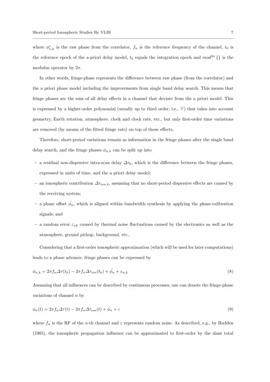
of kilometers. Figure 1 shows the typical VLBI signal flow at each station. Generally radio signals

(RF frequencies) caught by the antenna and amplified by the low noise amplifier (LNA) are mixed

with a local oscillator (LO) signal, which is phase-locked to a frequency standard, and then are down-

converted to an intermediate frequency (IF) signal, which lowers transmission losses efficiently as the

signal passes through the coaxial cables.

Figure 1 near here

In the next stage, the IF signal is separated into several channels and down-converted to baseband

frequencies (also called video frequencies, as conversion is done by video converters) ranging from zero

to several MHz. The video signal in each channel is then converted from an analog signal to a digital

one by the analog/digital (A/D) converter. Later the digitized signal is tagged with timing marks

within the formatter section of the data recorder. The formatter prepares the signal for recording and

sends it to the recorder (i.e., tape drive or hard disc). Recently, experiments aiming at (near) real-time

VLBI were carried out (e.g., Koyama et al. (2005)).

Correlation basically involves integration and multiplication operations on the digital signals, which

are sent from the two separate stations to the correlator center or are buffered on disks/tapes before


transferring the data, and is done either by a hard-wired correlator or by software (software correlator;

see Kondo et al. (2004)), capable of performing the same tasks.

The following section will briefly summarize the basics of correlation and discuss the method by

which fringe-phase information used for this study is obtained.

1.3 Correlator and its output

The correlator is used to integrate the correlation function every one (or two) seconds (as in geodetic

experiments) by making continuous corrections to the signal data stream in order to compensate for

variations in delay and Doppler shift due to the rotation of the Earth. There are two types of correlators:

the XF type correlator first performs the multiplication operation, then uses a Fourier transform to

convert the resulting cross-correlation function from the time domain to the frequency domain. The

FX type correlator first performs the Fourier transform of each data stream and then multiplies these

outputs with each other (Zensus et al. 1995).

The XF correlator was developed to achieve higher processing speed and is used for geodetic

applications. Following Takahashi et al. (2000), the cross-correlation function after fringe stopping

(i.e., mixing the received signal with a local oscillator frequency, which is equivalent to the Doppler

shift caused by Earth rotation) can be written by

R(τ) = Rr(τ)±Ri(τ) (1)

where the positive sign is valid for τ < 0 and the negative one for τ > 0. The real (Rr(τ)) and imaginary

(Ri(τ)) parts of the correlation function can be computed by Fourier transform as

Rr(τ) =12

[U(τ) + L(τ)] (2)

Ri(τ) = −12j [U(τ)− L(τ)] (3)

where

U(τ) =∫ [

X(f − fr)ejφ0 · Y ∗(f)]ej2πfτdf (4)

L(τ) =∫ [

X(f + fr)e−jφ0 · Y ∗(f)]ej2πfτdf (5)


were introduced. X(f) and Y (f) represent the Fourier transformed signals x(t) and y(t) received at

stations X and Y. The fringe rotation frequency (fr = f τ) can be computed from the a priori model,

and φ0 represents an initial phase at the beginning of the scan.

Fringe stopping can be performed either in the baseband or in the video band center. Usually the

latter approach is used since it has the advantage that correlation losses during fringe stopping are

only about 3.4% (Thompson et al. 2001). The video cross-spectrum Sv(j, k, n) for the n−th channel

serves as a basis for the coarse search function in order to determine delay and delay rate for each

channel.

F (n,∆τ, ∆τ) =1K

K∑

k=1

1J − 1

J−1∑

j=1

Sv(j, k, n)e−j2πfvj ∆τ

· e−j2πfn

0 ∆τ∆t k (6)

where k stands for the index of the individual integration (as mentioned in the beginning of this

section), j acts as an index for the frequency bin within the video band and ∆t reflects the duration

of the individual integrations. Values ∆τ, ∆τ that maximize Eq. (6) are added to the a priori model,

a process called single-band delay search (Takahashi et al. 2000).

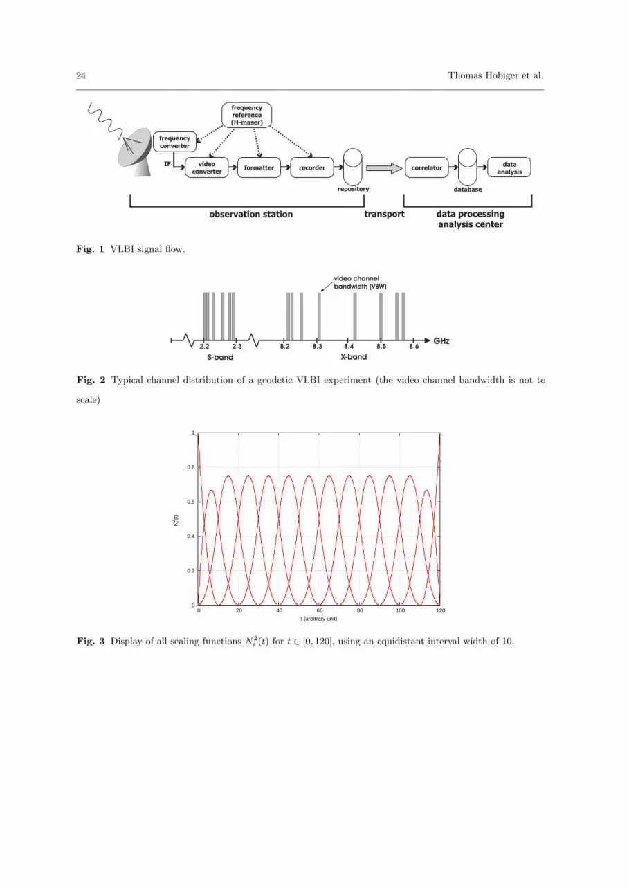
Geodetic observations are carried out at several channels within two distinct frequency bands in

order to achieve higher precision in the group delay measurements (Fig. 2). Thus, aligning data from

all channels with the help of the phase calibration (PCAL) signals and performing a multi-band delay

search (called bandwidth synthesis) gives the group delay observables for X- and S-band, which are

the input values for ensuing geodetic analysis (Takahashi et al. 2000).

Fig. 2 near here

1.4 Fringe phase and its information content

After correlation of the VLBI signals, a single-band delay search provides delay ∆τ and delay rate ∆τ ,

which can be used to update the a priori values used for correlation. The so-called (residual) fringe

phase φn,k for channel n and parameter period k is given by

φn,k = φcn,k −mod2π {2πfn[∆τ + ∆τ(tk − t0)]} (7)


where φcn,k is the raw phase from the correlator, fn is the reference frequency of the channel, t0 is

the reference epoch of the a-priori delay model, tk equals the integration epoch and mod2π {} is the

modulus operator by 2π.

In other words, fringe-phase represents the difference between raw phase (from the correlator) and

the a priori phase model including the improvements from single band delay search. This means that

fringe phases are the sum of all delay effects in a channel that deviate from the a priori model. This

is expressed by a higher-order polynomial (usually up to third order, i.e.,...τ ) that takes into account

geometry, Earth rotation, atmosphere, clock and clock rate, etc., but only first-order time variations

are removed (by means of the fitted fringe rate) on top of those effects.

Therefore, short-period variations remain as information in the fringe phases after the single band

delay search, and the fringe phases φn,k can be split up into

– a residual non-dispersive intra-scan delay ∆τk, which is the difference between the fringe phases,

expressed in units of time, and the a priori delay model;

– an ionospheric contribution ∆τion,k, assuming that no short-period dispersive effects are caused by

the receiving system;

– a phase offset φn, which is aligned within bandwidth synthesis by applying the phase-calibration

signals; and

– a random error εnk caused by thermal noise fluctuations caused by the electronics as well as the

atmosphere, ground pickup, background, etc..

Considering that a first-order ionospheric approximation (which will be used for later computations)

leads to a phase advance, fringe phases can be expressed by

φn,k = 2πfn∆τ(tk)− 2πfn∆τion(tk) + φn + εn,k (8)

Assuming that all influences can be described by continuous processes, one can denote the fringe-phase

variations of channel n by

φn(t) = 2πfn∆τ(t)− 2πfn∆τion(t) + φn + ε (9)

where fn is the RF of the n-th channel and ε represents random noise. As described, e.g., by Budden

(1985), the ionospheric propagation influence can be approximated to first-order by the slant total


electron content (STEC) along the ray path

τion =40.308cf2

S∫

R

ne(s) ds =40.308cf2

STEC (10)

where c is the speed of light (m s−1) and ne(s) represents the electron density (electrons m−3 ) along

the ray path between R and S. STEC is measured in total electron content units (TECU), where 1

TECU = 1016 electrons m−2.

For observations over a baseline between stations A and B,

∆τion(t) =40.308cf2

[STECA(t)− STECB(t)] =40.308cf2

∆STEC(t). (11)

Thus, the difference of the ionospheric conditions between station A and B determines the ionospheric

delay. Therefore Eq. (9) can be re-written as

φn(t) = 2πfn∆τ(t)− 2π40.308cfn

∆STEC(t) + φn + ε . (12)

Equation (12) reveals that all time-variable influences on intra-scan phases are either proportional

(residual delay) or inversely proportional (TEC) to the frequency of the concerned channel. Pure

phase variations, independent of channel frequency, are thought to be negligible as they are mainly

caused by frequency drifts of the oscillator, which is assumed to be stable within one scan of usually

60s to 300s (as for the scan analyzed in section 3, this requirement was verified by checking phase

calibration signals.).

For longer scans, changes in the room temperature might evoke a drift of the frequency standard,

which leads to a non-dispersive delay-like phase variation within the channel. In such cases, it is possible

to detect and remove such phase variations by utilizing PCAL phases. Using single channel data only,

it is impossible to separate ionospheric contributions from delay changes.

However, if fringe phases can be computed for individual channels, it becomes possible to distinguish

the ionospheric effects as they are scaled by the corresponding channel frequency. Using a proper but

simple model, which is able to deal with time variations as described above, it will become possible to

estimate these effects by an adjustment process.


1.5 Functional model for intra-scan delay variations

Short-period ionospheric variations (periods up to some tens of minutes) are expected not to happen

suddenly, but are thought to be phenomena that develop steadily or show continuous changes of TEC

(Afraimovich et al. 2004). The corresponding excitations have many physical causes arising in the

solar-terrestrial environment and cover geomagnetic disturbances, solar variations, and gravity waves,

which are caused by earthquakes, tsunamis (Ducic et al. 2003) or rocket launches (Afraimovich et al.

2000). Therefore, any descriptive model of ∆STEC and ∆τ(t) should be a continuous, smooth and

easy-to-implement function.

In the following, we use the quadratic B-spline N2(t) as a function of which the scaling coefficients

are determined by an adjustment process, since it fulfills above conditions and is easy to implement.

The advantages of this approach are discussed by e.g., Ogden (1997) or Schmidt (2001).

Given positive integers d and k, with k ≥ d, and a collection of non-decreasing values t0, t1, . . . , tk+d+1

called knots, the non-uniform B-spline basis functions of degree d are defined recursively as follows

(Stollnitz et al. 1995). For i = 0, 1, . . . , k, and for r = 1, 2, . . . , k, let

N0i (t) =

1 if ti ≤ t < ti+1

0 otherwise

(13)

Nri (t) =

t− titi+r − ti

Nr−1i (t) +

ti+r+1 − t

ti+r+1 − ti+1Nr−1

i+1 (t) (14)

(Note: The fractions in Eq. (14) are set to zero when their denominators are zero). So-called endpoint-

interpolating B-splines of degree d on the interval [TA, TB ] can be achieved when the first and last

d + 1 knots are set to TA and TB , respectively.

Figure 3 near here

Figure 3 shows an example of endpoint-interpolating quadratic B-splines, assuming t ∈ [0, 120]

and an equidistant interval width of 10. For our purposes, we use quadratic B-splines N2i (t) and

set t ∈ [0, Tscan] seconds, where Tscan denotes the scan duration. Usually the time resolution of fringe

phases is set by the correlator and is chosen to be one or two seconds for geodetic applications. Software

correlators allow calculation of nearly any integration time, but signal to noise ratio (SNR) should be


high enough to allow phase connection. The number of intervals can be set in accordance with the

expected frequency content.

For our studies, we used an interval length of 20s to detect even smallest ionospheric and instru-

mental variations. Thus, we set L = ceil(Tscan/20) (where ceil(x) gives the smallest integer greater

than or equal to x) and obtain the functional model for adjustment (using Eq. (12)).

φn(t) = 2πfn

L∑

l=0

Al ·N2l (t)− 2πC

fn

L∑

l=0

Bl ·N2l (t) + φn (15)

with the constant C = 40.308/c; Al represents the unknown coefficients of the residual intra-scan delay

and Bl those for ∆STEC.

The phase offsets φn can be determined together with the other unknowns in the adjustment

process. Fringe-phase information from several channels is necessary to separate these effects from

each other and to obtain reliable and robust results. When M represents the number of channels, then

the number u of unknown coefficients is given by

u = 2 · L + M − 2 (16)

The last term of Eq. (16) can be explained by the fact that phase offsets can only be estimated for

M −2 channels, since constant terms in the quadratic B-spline models for the residual intra-scan delay

and the ionosphere variation can be treated as phase offsets for two individual channels. As a convention

for dual-band observations (see the example given in section 3, using 14 channels, distributed over two

bands), we have chosen the first channel of each band to be free of phase offsets.

1.6 Stochastic model for intra-scan delay variations

The weighting of each fringe phase data-point is important since fringe phase quality can be degraded

within a scan by a myriad of instrumental effects (e.g., Petrov (2000) and Ray and Corey (1991)). As

described, e.g., by Takahashi et al. (2000), the standard deviation of phase measurements is inversely

proportional to their signal-to-noise ratio (SNR)

σφ =1

SNR(17)


The SNR is computed from the correlation amplitude ρ0 (i.e., the absolute values of the complex

correlation function, already compensated for sampling losses), the recorded bandwidth B and the

integration length ∆t as follows

SNR = ρ0

√2B∆t (18)

Since the SNR also takes into account that the last fringe phase data-point of a scan can be shorter

than the nominal integration period, we use SNR information to set up the weight matrix for the

adjustment process. Since the weights are inversely proportional to the variances, we get

Pxy =

SNR2xy (x = y)

0 (x 6= y)

. (19)

for the weight matrix.

Equation (18) points out that geodetic VLBI experiments are usually not a good source for the

accurate detection of ionospheric disturbances from fringe-phase data. Geodetic VLBI sessions are

scheduled in a way that as many as possible sources are tracked at different elevations in order to

separate clock, troposphere and station height (Boehm et al. 2002) within geodetic analysis (Sovers et

al. 1998). Thus, each source is only scheduled to track until a target SNR is reached.

On the one hand, since SNR ∼ √T , weak sources are tracked longer to reach desired SNR limits,

but the fringe-phase scatter is large and it becomes difficult to extract any useful signals from the

data. On the other hand, when a strong source is observed, SNR goals are reached after several tens

of seconds. Although the fringe-phase would be stable enough to detect dispersive effects and residual

intra-scan delay signals, the scan duration would be just too short to conclude on any physical causes.

1.7 Fitting the model parameters

Since Eq. (15) is linear in the unknown parameters Al, Bl, and φn, a least-squares adjustment following

a Gauss-Markov model (e.g., Koch (1997)), using the stochastic model introduced in section 1.6, can

be carried out. Additionally, formal errors of the estimated parameters can be computed and it is

possible to investigate how the different parameters are correlated with each other. All initial values


of the unknowns are set to zero and the o − c (observed minus calculated) vector just contains the

observations, i.e., the fringe-phases from all channels.

2 Ionosphere and TIDs

According to Hargreaves (1992), the ionosphere refers to the ionized part of the atmosphere that

contains significant numbers of free electrons and positive ions that exert a great influence on the

medium’s electrical properties. This means that all radio waves traveling through the ionosphere are

affected by a change in their propagation characteristics. The medium as a whole is electrically neutral

and contains equal numbers of positive and negative charges. Although the charged particles may be

only a minority amongst the neutral ones, they exert a great influence on the medium’s electrical

properties, and herein lies their importance.

Studies of the ionosphere have been carried out for a long time, and most of the characteristics

are now fairly well understood and can be explained by physical and chemical processes of the upper

atmosphere. The Earth’s ionosphere is strongly related to solar activity and the behavior of the geo-

magnetic field. Many measurements have been made using different techniques from locations around

the world, in order to understand the complex relationship that exists between solar conditions, the

geomagnetic field, geographic location, time of day, season, etc.. The most important time and spatial

variations are discussed by, e.g., Hakegard (1995) and the next section summarizes the features of

short-period disturbances that are expected to be detectable from VLBI fringe-phase data.

2.1 Traveling ionospheric disturbances

Traveling ionospheric disturbances (TIDs) manifest themselves as wavelike irregularities in ionospheric

parameters, such as electron density, electron temperature, ion temperature, etc.. Periods are from 10

min to several hours, horizontal wavelengths are between 100 km and several thousand kilometres, and

horizontal speeds are between 100 ms−1 and 1000 ms−1. TIDs with periods of the order of one hour,

wavelengths of the order of 1000 km, and horizontal speeds higher than about 250 ms−1 are called

large-scale TIDs (LSTIDs), while those with periods of several tens of minutes, horizontal wavelengths


of several hundred kilometres, and speeds slower than about 250 ms−1 are called medium-scale TIDs

(MSTIDs).

TIDs have been investigated for more than 50 years, and they are thought to be ionospheric

manifestations of atmospheric gravity waves (AGWs) (e.g., Hunsucker (1982)). In particular, LSTIDs

are considered to be formed from AGWs that are generated in the auroral zone of the Northern and

Southern Hemisphere by energy input from the magnetosphere and propagate towards a lower latitude

region. Hence they are important subjects to clarify the energy flow from the magnetosphere to the

low-latitude ionosphere.

Regarding MSTIDs, some researchers think that they are generated in the auroral zone like LSTIDs,

while some believe that they are phenomena attributed to meteorological processes. AGWs can be

generated from any causes that disturb the atmosphere. TIDs generated by a large earthquake have

been also reported recently (Heki and Ping 2005).

2.2 Plasma bubbles, blobs and ionospheric scintillations

Plasma bubbles, plasma blobs and ionospheric scintillations cause TEC variations that have a time-

scale less than that of TIDs. Plasma bubbles, in which plasma density is lower than that of the ambient

ionosphere, have a spatial scale of about 100 km and drift with the speed of a few 10 ms−1 to 100

ms−1 (e.g., Aarons (1993)). They are sometimes observed as a TEC variation event with a time-scale

of several minutes.

Plasma blobs, in which plasma density is higher than the ambient ionosphere, are events accompa-

nied by the quasi-periodic scintillations, and they produce TEC variations with a time scale of several

to several tens of minutes (Maruyama 1991).

Ionospheric scintillations are more short time-scale phenomena (e.g., Bhattacharyya and Rastogi

(1991)).


3 Detection of short-period TEC variations by VLBI

In this section, it will be shown how VLBI can detect small variations of TEC and how well these

findings agree with GPS measurements. As an example, a scan of the VLBI experiment SYW031 on

August 18th, 2004 on the baseline SYOWA (Antarctica) - HOBART26 (Australia) is taken (Fig. 4).

3.1 VLBI data

Data were obtained in the KOMB format (Takahashi et al. 1991), which contains not only the results of

bandwidth synthesis processing, but also fringe phases and SNR values for each parameter period and

channel. As phases are only measured between 0 and 2π, it might be necessary to unwrap the fringe

phases first, i.e., to carry out phase connection between the individual integrations. A TEC variation

of about 0.8 TECU is equal to 0.5 cycles at S-band, but only one eighth of a cycle in X-band.

As the KOMB data used for this study have an integration period length of 2s, TEC variations of

0.2 TECU/sec are assumed to be detectable when phase unwrapping is done properly. One limitation is

that if the observed sources have low flux densities, thus producing low SNR detections, the intra-scan

phases will show large scatter. As described in section 1.6, geodetic observables can still be obtained

from such sources if the scan is long enough, as the SNR scales by the square root of the scan length.

However, with large scatter in the fringe-phase data, phase unwrapping becomes impossible.

The strong source 1921-293 (unresolved S-band flux 5.4 Jy, unresolved X-band flux 6.2 Jy as

mentioned in VLBA Calibrator list (2005)) was observed on the SYOWA-HOBART26 baseline on

August 18th, 2004 from 10:10:12 UT until 10:14:28 UT. Figure 5 shows the fringe phases for each

channel from that scan. The S-band channels (lower six plots of Fig. 5) reveal a common pattern,

which can also be seen from the X-band channels (upper eight plots of Fig. 5) with lower amplitude.

Dispersive effects, i.e., ionospheric intra-scan delay variations, are assumed to be the reason for this

behavior as dispersive effects scale by ∼ 1/f .

Figure 5 near here

To test the ionospheric signal content, the fringe phases of each channel were scaled by the corre-

sponding reference frequency and the autocorrelation was computed. Figure 6 shows the results of this

simple method, where the curves are displaced by an offset of 0.2 to improve readability. The autocor-


relation functions of the different channels have their local minima and maxima at the same time lags

and they agree well in scale. This means that a common signal can be verified, when each channel is

scaled by its corresponding reference frequency. Thus, the assumption of a rapid ionospheric variation

(which causes dispersive effects over all channels), occurring during that scan can be demonstrated.

Therefore, the fringe phase information of the eight X-band and six S-band channels provides the basis

for separation of the different influences by a least-squares adjustment as described in section 1.4.

Figure 6 near here

Although the variations can be assigned to different physical effects, the parameters are correlated

with each other (Fig. 7). The first columns contain the Bl parameters associated with ∆STEC, followed

by the Al parameters associated with ∆τ and the phase offsets in X- and S-band. It can be seen that

ionosphere variations can be de-correlated from delay changes, but each of them is correlated with the

phase offsets. Whereas the ∆STEC is correlated with S-band phase offsets, the delay variations contain

a correlation with X-band phase offsets. This can be explained by the physical nature of the effects.

As ionospheric influences scale inversely proportional to the frequency, lower frequencies are affected

more than higher ones. Delay changes scale in direct proportion to the frequency and therefore X-band

is more influenced than the S-band.

Figure 7 near here

Finally, it can be stated that X-band (and S-band) phase offsets are highly correlated with each

other, but show no correlation with S-band (X-band) phase offsets. The correlation between parameters

of ∆STEC and ∆τ is mainly due to the same number of parameters for each effect and can be reduced

by choosing longer interval lengths of the B-spline functions. Figure 8 displays the estimated variation

of differential TEC of the scan in TECU. The dashed lines represent the formal error of the adjusted

curve at the 1σ level. The fitted curve has a maximum of 0.4 TECU and a minimum of −0.3 TECU

and reveals two major features that will be useful for validation of the results.

Figure 8 near here

Firstly, the local minimum can be detected around 140s after the scan had started, i.e., at 10:11:52

UT, and secondly the last period-like half-width has a duration of about 100s. The estimated residual

intra-scan delay variations are shown in Fig. 9. One can see that a maximum delay change of only


about 7 picoseconds occurs, which is equal to about 0.36 radians at X-band frequencies. Computing

the correlation coefficient between ∆STEC variations and delay changes gives a value of 0.44.

Fig. 9 near here

In order to prove that the effects are of real nature and not just artifacts caused by the receiving

system, it will be necessary to find other techniques that can reveal the same effect. Therefore, GPS

data were analyzed with respect to TEC variations.

3.2 GPS data

GPS provides a tool for ionospheric-wave disturbance detection based on carrier-phase measurements

of slant TEC (e.g., Afraimovich et al. (2003)). The relation between STEC and carrier-phase measure-

ments carried out on L1 and L2 can be found, e.g., in Hofmann-Wellenhof et al. (2001).

STEC =1

40.308f21 f2

2

f21 − f2

2

[(L1λ1 − L2λ2) + const + nL] (20)

The additional paths of the radio signal (in metres) caused by the ionosphere are expressed by L1λ1

and L2λ2, where L1 and L2 represent the number of phase rotations at frequencies f1 and f2, and λ1

and λ2 stand for the corresponding wavelengths in metres.

The constant represents the unknown initial carrier-phase ambiguity and nL symbolizes errors in

determination of the phase path. If the basic GPS frequency f0 = 10.23 MHz is used, f1 and f2 can

be expressed by (Spilker 1978)

f1 = 154 · f0 f2 = 120 · f0 . (21)

The corresponding wavelengths can be computed, using the speed of light c, which relates frequency to

wavelength by c = λf . The data are usually stored in intervals of 30 seconds (or shorter) and provided

by Receiver Independent Exchange Format (RINEX) files to a broad user community.

In recent years, a lot of stations have been equipped with 1Hz GPS receivers, which makes it

possible to detect short-period disturbances of the ionosphere. Special GPS receivers, dedicated to

ionosphere research, have the ability to record data with sampling rates up to several Hz (Shilo et al.

2000). Carrier-phase measurements can be made very accurately and formal errors of the determined


STEC reach values of 0.01 TECU, if these special receivers are used (Ducic et al. 2003). Even for

geodetic GPS receivers, the error is expected not to exceed 0.1 TECU.

In order to handle GPS observations in RINEX format, the open-source GPSTK software package

(Tolman et al. 2004) was applied. Fortunately, the VLBI stations SYOWA and HOBART26 have co-

located GPS receivers that can be used for comparison. RINEX data at these stations were recorded

in time-steps of 30s, so that eight data-points correspond in time with the VLBI scan.

In order to compare GPS and VLBI STEC measurements, one has to select those satellites as seen

from each station that lie near the source observed in the VLBI scan on the plane of the sky. Thus,

sky-plots for stations SYOWA and HOBART26 were generated, including the tracked GPS satellites

and the radio source at each site (Figs. 10 and 11). At station HOBART26, GPS space vehicles (SV)

14 and 22 are closest to the pointing direction of the antenna (Fig. 10) and at SYOWA the SV 14

fulfills this spatial criterion (Fig. 11).

Figs. 10 and 11 near here

It can be expected that the ionosphere variations detected by VLBI can also be seen from dual-

frequency GPS measurements. Therefore, RINEX data for Internatioanl Global Navigation Satellite

System (GNSS) Service (IGS) station HOB2, which is located close to the VLBI antenna, was down-

loaded, geometry-free phase delay was computed, detrended and transformed into TECU. No signifi-

cant ionospheric variation could be seen around the epoch when the radio telescope was observing the

particular radio source.

The same procedure was applied for IGS station SYOG, which is the GPS receiver of the Antarctic

station Syowa. A strong variation of STEC, similar to that one observed by VLBI, can be detected by

GPS (Fig. 12).

Fig. 12 near here

3.3 Interpretation of the results

Other GPS signals than the one from SV 14 do not reveal the same pattern (SVs 7, 11, 28, 31), are

too noisy (SV 9), or have too many cycle slips (SV 20). Therefore, precise information about traveling


speed and propagation direction cannot be obtained. Nevertheless, several features of the ionospheric

disturbance can be deduced from VLBI and single GPS satellite observations:

1. A main feature of the ionospheric disturbance can be deduced from the VLBI and GPS results

(Figs. 8 and 12). The signature is detected first in the GPS signal and shows a time-delay ∆T of

about 240s before it affects the VLBI measurement.

2. Since VLBI and SV 14 are approximately oriented in the same azimuth (Fig. 11), we can use the

following formula to calculate the distance D between the intersection points of the rays with an

ionospheric shell at height H

D = (Re + H) ·[zv − zg − arcsin

(Re

Re + Hsin zv

)+ arcsin

(Re

Re + Hsin zg

)](22)

Figure 13 shows the basic geometry where Re represents the radius of a spherical Earth (6371km),

and zv and zg are the zenith distances (in radians) from VLBI and GPS measurements. When the

height of the disturbance is assumed to be at 250km, the spatial distance between the different

intersection points will be 246km. If the height is changed to H = 500km, the distance and the

follow on calculations of propagation speed will increase by about 50%. Since 250km represents an

average height at which ionospheric disturbances occur, we have chosen it for our further analysis.

3. Since VLBI and GPS measurements are aligned in a plane, we can compute the upper limit for an

estimate of the propagation speed by vmax = D/∆T , which is equal to the true velocity v when

the disturbance propagates exactly in the azimuth direction in which the antenna (and the GPS

satellite) points. Thus, we obtain v < vtextmax = 1028ms−1, which is in good agreement with recent

findings of fast-traveling disturbances (Hawarey 2006). The true propagation direction can scale

v proportional to ∼ vtextmax cosβ, where β represents the difference between the azimuth of the

propagation direction and the azimuth of the observation.

4. Since the disturbance is seen first in the GPS measurements before it affects the radio signals

received by the VLBI antenna, southward propagation direction can be assumed.

5. The amplitude measured by VLBI is slightly larger than that measured by GPS. This can be

explained by the fact that the VLBI observation is carried out at a lower elevation angle, which

causes a longer ray path through the ionosphere and thus a higher STEC value. The scaling between

the results can be explained well by ionosphere mapping functions (Schaer 1999).


6. A comparison of the VLBI and GPS STEC time-series reveals a difference in the duration of the two

sets of variations. By definition, the VLBI variations last about 250s, while the corresponding GPS

variation spans 320s. Considering that VLBI source motion follows East-West direction and the

GPS satellite is moving from North-West to South-East, having a West-East component helps to get

deeper understanding of the observed feature. Considering this and assuming a velocity component

v⊥ = 630ms−1 perpendicular to the azimuth direction could explain the different time-scales of the

variations as seen by VLBI and GPS.

Thus, a short period ionospheric disturbance propagating with a speed of ≤ 1000ms−1 is the

most likely explanation for the phase variations measured at SYOWA by VLBI and GPS. Considering

that location and the epoch of observation (10 UT) leads to the conclusion that the disturbance

originated around the auroral oval. Measurements of energetic auroral electrons (Fig. 14) encourage

this explanation.

Solar flux at 10.7cm (F10.7) and the terrestrial Kp index (SEC-NOAA 2006) show no clear hint

that explains the occurrence of this event. The day of the observation was magnetically quiet, but only

the interplanetary magnetic field (SEC-NOAA 2006) showed some evidence for a disturbance. The

International Magnetic Field (IMF) was directed southward before the measurements were carried out,

which permits interaction between the auroral ovals and the solar wind. Considering the dimension of

the event and the travelling speed, plasma patches are assumed to be the likely cause of the STEC

variations measured by VLBI and GPS. Propagation speed, time and location of the event agree well

with the characteristics of plasma patches as described by Ma and Schunk (2001).

4 Possible fields of application and requisites

It has been shown that VLBI is able to detect small, rapid variations of the ionosphere with a high time

resolution as the sampling rate of fringe phases is equal to the integration period (here 2s). As discussed

in section 1.6, strong sources are necessary to ensure high SNR in order to enable phase connection

and/or phase unwrapping. With such sources, it should be possible to detect all TEC variations of the

ionosphere, provided that the scan is long enough.


Since VLBI is a differential technique, time-dependent variations of ∆STEC cannot be clearly

assigned to a single station without external information (like GPS in the example here) or other mea-

surements. However, if two baselines connect one station, one can compute the ionospheric variations

from both measurements and check whether the same signals can be found.

VLBI has the large advantage that fringe phase information is very precise and that the formal error

of each measurement can be derived easily from the corresponding correlation amplitude. Therefore,

one can think of the following applications:

– Detection of TIDs.

– Detection of plasma bubbles (Sitnov et al. 2005).

– Monitoring diurnal TEC variations with high precision by VLBI experiments.

– Detection of ionospheric disturbances caused by earthquakes, tsunamis or rocket launches.

– Verifying the different reactions of the ionosphere to solar excitations and geomagnetic disturbances.

Besides applications specifically geared towards studying the ionosphere itself, the method de-

scribed in this paper would also provide a basis for handling intra-scan delay variations and providing

phase delay, which is at least one magnitude more precise than current group delay measurements, for

geodetic/astrometric purposes or for the navigation of spacecraft.

Acknowledgements We are very grateful to the Austrian Science Fund (FWF), which funded the research

project P16136-N06 ”Investigation of the ionosphere by geodetic VLBI”. Furthermore, we want to thank

the Japanese Society for the Promotion of Science, JSPS (projects PE04023 and P06603) for supporting

our research. The International VLBI Service for Geodesy and Astrometry (IVS), International GNSS Service

(IGS), and our colleagues from Kashima Space Research Center and Geographical Survey Institute (Japan) are

acknowledged for providing data. The Space Environment Center, US National Oceanographic and Atmospheric

Administration (NOAA) is acknowledged for providing space weather data and for release of Fig. 14. The

authors are grateful to Bob Campbell and Brian Corey for their critical comments and helpful suggestions,

which improved the manuscript greatly.

References

Aarons J (1993) The longitudinal morphology of equatorial F-layer irregularities relevant to their occurrence,

Space Science Reviews, 63(3/4), 209-243.


Afraimovich EL, Kosogorov EA, Palamarchouk KS, Perevalova NP, Plotnikov AV (2000) The use of GPS arrays

in detecting the ionospheric response during rocket launchings, Earth Planets Space, 52(11), 1061-1066.

Afraimovich EL, Perevalova NP, Voyeikov SV (2003) Traveling wave packets of total electron content distur-

bances as deduced from global GPS network data, Journal of Atmospheric and Solar-terrestrial Physics,

65(11), 1245-1262.

Afraimovich EL, Astafieva EI, Voyeikov SV (2004) Isolated ionospheric disturbance as deduced from global

GPS network, Annales Geophysicae, 22(1), 47-62, SRef:1432-0576/ag/2004-22-47.

Bhattacharyya A, Rastogi RG (1991) Structure of ionospheric irregularities from amplitude and phase scintil-

lation observations, Radio Science, 26, 439-449.

Boehm J, Schuh H, Weber R (2002) Influence of tropospheric zenith delays obtained by GPS and VLBI

on station heights. In: Vertical Reference Systems, H. Drewes,A.H. Dodson,L.P.S. Fortes, L. Sanchez, P.

Sandoval (Eds.), IAG Symposia Vol. 124, 107-112, Springer, Berlin, Heidelberg, New York.

Budden KG (1985) The propagation of radio waves, Cambridge University Press, Cambridge.

Ducic V, Artru J, Lognonne P (2003) Ionospheric remote sensing of the Denali Earthquake Rayleigh surface

waves, Geophysical Research Letters, 30(18), 1951-1958, doi:10.1029/2003GL017812.

Hakegard O (1995) A regional ionospheric model for real-time predictions of the total electron content in wide

area differential satellite navigation systems, PhD Thesis, Norwegian Institute of Technology, Norway.

Hargreaves JK (1992) The solar-terrestrial environment,Cambridge University Press, Cambridge.

Hawarey M (2006) Travelling ionospheric disturbance over California mid 2000, Journal of Nonlinear Processes

in Geophysics, 13 (1-), SRef-ID: 1607-7946/npg/2006-13-1, 2006.

Heki K, Ping J (2005) Directivity and apparent velocity of the coseismic ionospheric disturbances observed with

a dense GPS array, Earth and Planetary Science Letters, 236(3-4), 845-855, doi:10.1016/j.epsl.2005.06.010.

Hobiger T, Kondo T, Schuh H (2006) Very long baseline interferometry as a tool to probe the ionosphere,

Radio Sci., 41, RS1006, doi:10.1029/2005RS003297.

Hobiger T (2006) VLBI as a tool to probe the ionosphere, PhD thesis, Vienna University of Technology, pub-

lished under: Schriftenreihe der Studienrichtung Vermessung und Geoinformation, Technische Universitaet

Wien, ISSN 1811-8380.

Hofmann-Wellenhof B, Lichtenegger H, Collins J (2001) Global Positioning System - Theory and Practice, 5th

ed, Springer, Berlin, Heidelberg, New York.

Hunsucker RD (1982) Atmospheric gravity waves generated in the high-latitude ionosphere: A review, Rev.

Geophys., 20(2), 293-315.

Jacobson AB, Erickson WC (1993) Observations of electron-density irregularities in the plasmasphere using

the VLA radio-interferometer. Annales de Geophysique, 11, 869-73.

Kassim NE, Perley RA, Erickson WC, Dwarakanath KS (1993) Subarcminute resolution imaging of radiosources

at 74 MHz with the very large array, Astron. J., 106, 2218-2228.


Koch KR (1997) Parameter Estimation and Hypothesis Testing in Linear Models, Springer, Berlin, Heidelberg,

New York.

Kondo T, Kimura M, Koyama Y, Osaki H (2004) Current Status of Software Correlators Developed at Kashima

Space Research Center, International VLBI Service for Geodesy and Astrometry 2004 General Meeting

Proceedings, NASA/CP-2004-212255, 186-190.

Koyama Y, Kondo T, Osaki H, Whitney AR, Dudevoir KA (2005) Rapid Turnaround EOP Measurements

by VLBI over the Internet,Sanso F (ed), A Window on the Future of Geodesy, 119-124, Springer, Berlin,

Heidelberg, New York.

Ma T, Schunk RW (2001) The effects of multiple propagating plasma patches on the polar thermosphere,

Journal of Atmospheric and Solar-Terrestrial Physics, 63(4), 355-366, doi:10.1016/S1364-6826(00)00181-4.

Maruyama T (1991) Observations of quasi-periodic scintillations and their possible relation to the dynamics

of ES plasma blobs, Radio Science, 26, 691-700.

Ogden RT (1997) Essential Wavelets for Statistical Applications and Data Analysis, Birkhauser, Boston.

Petrov L (2000) Instrumental Errors of Geodetic VLBI, in International VLBI Service for Geodesy and Astrom-

etry 2000 General Meeting Proceedings, Vandenberg NR and Baver KB (eds.), NASA/CP-2000-209893.

Ray JR, Corey BE (1991) Current Precision of VLBI Multi-Band Delay Observables, Proceedings AGU Chap-

man Conference on Geodetic VLBI: Monitoring Global Change, Washington D.C., 22-26 April.

Roberts DH, Klobuchar JA, Fougere PF, Hendrickson DH (1982a) A large-amplitude traveling ionospheric

disturbance produced by the May 18, 1980, explosion of Mount St. Helens, Journal of Geophysical Research,

87, 6291-6301.

Roberts DH, Rogers AEE, Allen BR, Bennett CL, Burke BF, Greenfield PE, Lawrence CR, Clark T (1982b)

Radio interferometric detection of a traveling ionospheric disturbance excited by the explosion of Mount

St. Helens, Journal of Geophysical Research, 87, 6302-6306.

Schaer S (1999) Mapping and Predicting the Earth’s Ionosphere Using the Global Positioning System, Ph.D.

thesis, Bern University.

Schmidt M (2001) Basis principles of wavelet analysis and applications in geodesy (in German), Post-doctoral

thesis, Shaker, Aachen, Germany.

Space Environment Center, Boulder, CO, National Oceanic and Atmospheric Administration, US Dept. of

Commerce (2006) http://www.sec.noaa.gov/index.html

Shilo NM, Essex EA, Breed AM (2000) Ionospheric Scintillation Study of the Southern High Latitude Iono-

sphere, WARS’00- Workshop on the Applications of Radio Science, National Committee for Radio Science,

Australia, 154-159.

Sitnov MI, Guzdar PN, Swisdak M (2005) On the formation of a plasma bubble, Geophysical Research Letters,

32(16103), doi:10.1029/2005GL023585.


Sovers OJ, Fanselow JL, Jacobs CS (1998) Astrometry and geodesy with radio interferometry: experiments,

models, results., Reviews of Modern Physics, 70(4), 1393-1454.

Spilker JJ (1978) GPS Signal Structure and Performance Characteristics, Journal of Navigation, 25(2), 121-146.

Stollnitz EJ, DeRose TD, Salesin DH (1995) Wavelets for computer graphics: A primer, part 2, IEEE Computer

Graphics and Applications, 15(4), 75-85.

Takahashi Y, Hama S, Kondo T (1991) K-3 software system for VLBI and new correlation processing software

for K-4 recording system, Journal of the Communications Research Laboratory, 38(3), 481-502.

Takahashi F, Kondo T, Takahashi Y, Koyama Y (2000) Very Long Baseline Interferometer, Ohmsha, Japan.

Thompson AR, Moran JM, Swenson GW (2001) Interferometry and Synthesis in Radio Astronomy, John Wiley

& Sons, New York.

Tolman B, Harris RB, Gaussiran T, Munton D, Little J, Mach R, Nelsen S, Renfro B, Schlossberg D (2004)

The GPS Toolkit – Open Source GPS Software, Proceedings of the 17th International Technical Meeting

of the Satellite Division of the Institute of Navigation, ION GNSS 2004, 2044-2053.

VLBA Calibrator list (2005), Version Dec 15, 2005, http://www.vlba.nrao.edu/astro/calib/vlbaCalib.txt.

Zensus JA, Diamond PJ, Napier PJ (eds.) (1995) Very Long Baseline Interferometry and the VLBA, ASP

Conference Series Vol. 82, Astronomical Society of the Pacific, San Francisco, ISBN 1-886733-02-3.


Fig. 1 VLBI signal flow.

Fig. 2 Typical channel distribution of a geodetic VLBI experiment (the video channel bandwidth is not to

scale)

0

0.2

0.4

0.6

0.8

1

0 20 40 60 80 100 120

N2 i (

t)

t [arbitrary unit]

Fig. 3 Display of all scaling functions N2i (t) for t ∈ [0, 120], using an equidistant interval width of 10.


Fig. 4 Baseline SYOWA (Antarctica) - HOBART26 (Australia); Lambert conic conformal projection.

6

4

2

0 200 100 0

8.21099 GHz

6

4

2

0 200 100 0

8.22099 GHz

6

4

2

0 200 100 0

8.25099 GHz

6

4

2

0 200 100 0

8.31099 GHz

6

4

2

0 200 100 0

8.42099 GHz

6

4

2

0 200 100 0

8.50099 GHz

6

4

2

0 200 100 0

8.55099 GHz

6

4

2

0 200 100 0

8.57099 GHz

6

4

2

0 200 100 0

2.20799 GHz

6

4

2

0 200 100 0

2.21299 GHz

6

4

2

0 200 100 0

2.22799 GHz

6

4

2

0 200 100 0

2.25799 GHz

6

4

2

0 200 100 0

2.28299 GHz

6

4

2

0 200 100 0

2.29299 GHz

Fig. 5 Fringe phases (0 . . . 2π) on baseline SYOWA-HOBART26 from experiment SYW031, August 18th, 2004

from 10:10:12 UT until 10:14:28 UT, having an integration period of 2s.


-0.5

0

0.5

1

1.5

2

2.5

3

3.5

4

0 50 100 150 200 250

time [s]

Frequency [Hz]8.21099e+098.22099e+09 8.25099e+098.31099e+098.42099e+098.42099e+098.50099e+098.57099e+092.20799e+092.21299e+092.22799e+092.25799e+092.28299e+092.29299e+09

Fig. 6 Autocorrelation of the fringe-phase information, scaled by reference frequency. Individual channels are

offset by 0.2 to improve legibility.

0

0.2

0.4

0.6

0.8

1

off.Soff. Xτ∆STEC

off.S

off. X

τ

∆STEC

Fig. 7 Absolute values of the correlation coefficients between the estimated parameters.


-0.4

-0.2

0

0.2

0.4

0.6

0 50 100 150 200 250

∆ S

TE

C [T

EC

U]

time [s]

Fig. 8 Intra-scan variation of ∆STEC in TECU on August 18th, 2004 from 10:10:12 UT until 10:14:28 on the

baseline SYOWA-HOBART26. Formal error at 3σ level is displayed by dashed lines.

-0.01

-0.008

-0.006

-0.004

-0.002

0

0.002

0.004

0.006

0.008

0.01

0 50 100 150 200 250

τ [n

s]

time [s]

Fig. 9 Intra-scan variation of τ in nanoseconds on August 18th, 2004 from 10:10:12 UT until 10:14:28 on the

baseline SYOWA-HOBART26. Formal error at 3σ level is displayed by dashed lines.


90

75

60

45

30

15

15

30

45

60

75

90

907560453015153045607590

1921-293

SV 01SV 03SV 09SV 11SV 14SV 15SV 18SV 19SV 22SV 25

Fig. 10 Sky-plot for station HOBART26 (asterisks denote GPS satellites, the cross indicates the direction to

the radio source).

90

75

60

45

30

15

15

30

45

60

75

90

907560453015153045607590

1921-293

SV 07SV 09SV 11SV 14SV 20SV 28SV 31

Fig. 11 Sky-plot for station SYOWA (asterisks denote GPS satellites, the cross indicates the direction to the

radio source).


-0.4

-0.2

0

0.2

0.4

0.6

-300 -200 -100 0 100 200

ST

EC

[TE

CU

]

time [s]

Fig. 12 STEC at station SYOG, computed between receiver and GPS SV 14. The dashed line represents the

observed STEC from VLBI, which is shifted and scaled in order to compensate for the geometry (see discussion

in section 3.3). One has to bear in mind that GPS data is obtained every 30s.

Fig. 13 Description of the geometric situation for the computation of the propagation speed of the ionospheric

disturbance. Re represents the radius of a spherical Earth (6371km), H the height of the ionospheric layer and zv

and zg are the zenith distances (in radians) from VLBI and GPS measurements. The corresponding geocentric

angle αv can be computed by αv = zv − arcsin(

ReRe+H

sin zv

). The angle αg is obtained in the same way.


Fig. 14 The display of the statistical auroral oval (color-coded to the bar on the right hand side in erg cm−2

s−1) includes a presentation of the actual auroral energy input observations that were used to estimate the

hemispheric power and the level of auroral activity. This presentation shows the track of NOAA-17 (one of the

series of polar orbiting meteorological satellites) over the polar region. The length of the solid line indicates

that amount of energy into the atmosphere that was observed at that point along the satellite track. The scales

in the four corners of the plot may be used to convert the line length to actual energy flux. The length of the

dotted line is an indication of the energy of the electrons that are flowing into the atmosphere to produce the

aurora. A line of two dots represents a very low energy of about 100 eV, a length of 16 dots a high energy.

Both the solid and dotted lines are plotted every 16s or about 100km along the satellite track (on courtesy of

NOAA).

Documents

Using VLBI fringe-phase information from geodetic experiments for short-period ionospheric studies