Embed Size (px)
Citation preview
HAL Id: tel-01684784https://tel.archives-ouvertes.fr/tel-01684784
Submitted on 15 Jan 2018
HAL is a multi-disciplinary open accessarchive for the deposit and dissemination of sci-entific research documents, whether they are pub-lished or not. The documents may come fromteaching and research institutions in France orabroad, or from public or private research centers.
L’archive ouverte pluridisciplinaire HAL, estdestinée au dépôt et à la diffusion de documentsscientifiques de niveau recherche, publiés ou non,émanant des établissements d’enseignement et derecherche français ou étrangers, des laboratoirespublics ou privés.
Variabilité démographique et adaptation de la gestionaux changements climatiques en forêt de montagne :
calibration par Calcul Bayésien Approché et projectionavec le modèle Samsara2
Guillaume Lagarrigues
To cite this version:Guillaume Lagarrigues. Variabilité démographique et adaptation de la gestion aux changements cli-matiques en forêt de montagne : calibration par Calcul Bayésien Approché et projection avec le modèleSamsara2. Sciences de la Terre. Université Grenoble Alpes, 2016. Français. �NNT : 2016GREAV081�.�tel-01684784�
THÈSEPour obtenir le grade de
DOCTEUR DE LA COMMUNAUTÉ UNIVERSITÉ GRENOBLE ALPESSpécialité : Biodiversité Écologie EnvironnementArrêté ministériel : 7 Août 2006
Présentée par
Guillaume Lagarrigues
Thèse dirigée par Benoît Courbaudet codirigée par Franck Jabot
préparée au sein Unité EMGR d’IRSTEA Grenobleet de Ecole Doctorale Chimie et Sciences du Vivant
Variabilité démographique et adaptationde la gestion aux changements climatiquesen forêt de montagne : calibration parCalcul Bayésien Approché et projectionavec le modèle Samsara2
Thèse soutenue publiquement le 16 décembre 2016devant le jury composé de :
Dr Harald BugmannProfesseur, ETH Zürich, RapporteurDr Bruno HéraultCharge de recherche, CIRAD, UMR Ecofog, RapporteurDr Eric DufrêneDirecteur de recherche, CNRS, Laboratoire Ecologie Systématique et Evolution (UMR 8079), ExaminateurDr Olivier FrançoisProfesseur, UGA, laboratoire TIMC-IMAG, Président Dr Benoît CourbaudIngénieur-chercheur, HDR, IRSTEA Grenoble, Directeur de thèseFranck JabotIngénieur-chercheur, HDR, IRSTEA Clermont-Ferrand, Co-Directeur de thèse1

22
Résumé
Les hêtraies-sapinières-pessières de montagne paraissent particulièrement menacées par le réchaufe-ment climatique. Pour appréhender la dynamique future de ces forêts et adapter la sylviculture à cesnouvelles conditions, il est important de mieux connaître les facteurs environnementaux impactant ladémographie de ces espèces. Nous avons abordé cette problématique en combinant des données his-toriques de gestion, le modèle de dynamique forestière Samsara2 et une méthode de calibration baséesur le Calcul Bayésien Approché. Nous avons ainsi pu étudier conjointement les diférents processusdémographiques dans ces forêts. Nos analyses montrent que la démographie forestière peut varier forte-ment entre les parcelles et que le climat n’est pas toujours déterminant pour expliquer ces variations.Ainsi, malgré les changements climatiques attendus, la gestion irrégulière pratiquée actuellement de-vrait permettre de maintenir les services rendus par les peuplements mélangés situés en conditionsmésiques.
Mots clés
Démographie forestière ; Picea abies ; Abies alba ; Fagus sylvatica ; Approximate Bayesian Compu-tation ; Réchaufement climatique
Abstract
The spruce-ir-beech mountain forests could be particularly threatened by global warming. To betterunderstand the future dynamics of these forests and adapt the silviculture to these new conditions, abetter knowledge of the environmental factors afecting species demographics is needed. We studiedthis issue by combining a historical management data set, the forest dynamics model Samsara2 anda calibration method based on Approximate Bayesian Computation. We were able thus to studyjointly diferent demographic process in these forests. Our analysis show that forest demographics canstrongly vary between stands and that climate is not always determining to explain these variations.Thus, despite the expected climate changes, the uneven-aged management currently applied mightallow to preserve the services provided by the mixed stands located in mesic conditions.
Key words
Forest demographics ; Picea abies ; Abies alba ; Fagus sylvatica ; Approximate Bayesian Computation; Global warming
33

Remerciements
Je souhaite remercier pour commencer mes directeurs de thèse, Benoît Courbaud et Franck Jabot,pour leur soutien tout au long de ces trois années. J’ai apprécié tout autant l’autonomie qu’ils m’ontlaissé dans mon travail que leur implication et leur réactivité quand j’en ai eu besoin.
J’ai beaucoup apprécié ma vie professionnelle au sein de l’unité Ecosystèmes Montagnards. J’ai trouvémotivant de pouvoir assister et participer aux séminaires EM, aller mesurer et trouer des arbres detemps en temps, participer aux refaisages de monde le midi au CTP, aider et être aider par les collègues,etc. Merci aussi à mes idèles compagnons de terrain, Sophie Labonne, Eric Mermin et Pascal Tardif,qui m’ont même accompagné jusque dans mes Pyrénées ariégeoises pour aller mesurer des arbres ! J’aiaussi une pensée plus particulière pour mes voisins de bureau, Marc, Sophie, Jean-Jacques, Jérémy,Thomas, Valentine, Anne-Léna, Lauric avec qui j’ai fait beaucoup de choses, au boulot et ailleurs !
Je voudrais également remercier les personnes de l’ONF avec qui j’ai interagi au cours de ces troisannées, en particulier Christine Deleuze, Didier François, Thierry Sardin et Catherine Riond pour lesaspects scientiiques, et Thomas Villiers, Jacques Fay, Georges Rivet, Patrick Guillon pour leur aidedans la collecte des documents d’archives et pour les discussions passionnantes que nous avons eues àpropos de ”leurs” forêts.
Merci aussi à Eric Maldonado pour son appui technique sur tout ce qui concerne l’informatique scien-tiique, et à Carine Soula pour sa relecture consciencieuse de l’ensemble de ce manuscrit !
Pour inir, je remercie l’ADEME et l’ONF d’avoir inancé ce projet de thèse.
44
Table des matières
1 - Préambule 8
2 - Introduction 92.1 Problématique générale et enjeux de recherche . . . . . . . . . . . . . . . . . . . . . . . 9
2.1.1 Problématique posée par les changements climatiques en forêt de montagne . . . 92.1.1.1 Observations et causes des changements climatiques et conséquences at-
tendues pour les écosystèmes au niveau mondial . . . . . . . . . . . . 92.1.1.2 Problématique pour les montagnes européennes . . . . . . . . . . . . . . 102.1.1.3 Cas des hêtraies-sapinières-pessières gérées . . . . . . . . . . . . . . . . 11
2.1.2 Démographie forestière . . . . . . . . . . . . . . . . . . . . . . . . . . . . . . . . . 132.1.2.1 Les diférents processus démographiques . . . . . . . . . . . . . . . . . . 132.1.2.2 Les facteurs écologiques inluençant la démographie forestière . . . . . . 14
2.1.2.2.1 Inluence des facteurs abiotiques . . . . . . . . . . . . . . . . . 142.1.2.2.2 Inluence des facteurs biotiques endogènes . . . . . . . . . . . . 172.1.2.2.3 Inluence des facteurs biotiques exogènes . . . . . . . . . . . . . 192.1.2.2.4 Inluence des facteurs anthropiques . . . . . . . . . . . . . . . . 19
2.1.2.3 Enjeu de recherche sur la démographie forestière . . . . . . . . . . . . . 202.1.3 Gestion forestière . . . . . . . . . . . . . . . . . . . . . . . . . . . . . . . . . . . . 20
2.1.3.1 Enjeux pour les forêts de montagne européennes . . . . . . . . . . . . . 202.1.3.2 Gestion de peuplements inéquiens . . . . . . . . . . . . . . . . . . . . . 212.1.3.3 Adaptation de la sylviculture au changement climatique . . . . . . . . . 212.1.3.4 Enjeu de recherche sur la gestion irrégulière . . . . . . . . . . . . . . . . 23
2.2 Données et outils d’analyse à disposition . . . . . . . . . . . . . . . . . . . . . . . . . . . 232.2.1 Les données historiques de gestion . . . . . . . . . . . . . . . . . . . . . . . . . . 232.2.2 La modélisation . . . . . . . . . . . . . . . . . . . . . . . . . . . . . . . . . . . . . 232.2.3 La modélisation de la dynamique forestière . . . . . . . . . . . . . . . . . . . . . 23
2.2.3.1 Considérations générales . . . . . . . . . . . . . . . . . . . . . . . . . . . 232.2.3.2 Le modèle Samsara2 . . . . . . . . . . . . . . . . . . . . . . . . . . . . . 24
2.2.4 Le Calcul Bayésien Approché (ABC) . . . . . . . . . . . . . . . . . . . . . . . . . 252.2.4.1 Présentation . . . . . . . . . . . . . . . . . . . . . . . . . . . . . . . . . 252.2.4.2 Principe de fonctionnement . . . . . . . . . . . . . . . . . . . . . . . . . 262.2.4.3 Enjeu de recherche sur la méthode ABC . . . . . . . . . . . . . . . . . . 27
2.2.5 La modélisation de la gestion forestière . . . . . . . . . . . . . . . . . . . . . . . . 282.2.5.1 Considérations générales . . . . . . . . . . . . . . . . . . . . . . . . . . . 282.2.5.2 Algorithme NV . . . . . . . . . . . . . . . . . . . . . . . . . . . . . . . . 282.2.5.3 Algorithme UMA . . . . . . . . . . . . . . . . . . . . . . . . . . . . . . . 30
2.2.6 La modélisation des facteurs écologiques . . . . . . . . . . . . . . . . . . . . . . . 312.3 Structuration de la thèse . . . . . . . . . . . . . . . . . . . . . . . . . . . . . . . . . . . 32
2.3.1 Objectifs . . . . . . . . . . . . . . . . . . . . . . . . . . . . . . . . . . . . . . . . . 322.3.2 Hypothèses de travail . . . . . . . . . . . . . . . . . . . . . . . . . . . . . . . . . 32
3 - Partie 1 : Origines et nature des données utilisées 343.1 Préambule . . . . . . . . . . . . . . . . . . . . . . . . . . . . . . . . . . . . . . . . . . . . 343.2 Origines et nature des données utilisées . . . . . . . . . . . . . . . . . . . . . . . . . . . 34
3.2.1 Données historiques de gestion . . . . . . . . . . . . . . . . . . . . . . . . . . . . 343.2.1.1 Généralités . . . . . . . . . . . . . . . . . . . . . . . . . . . . . . . . . . 343.2.1.2 Archives de gestion de l’ONF . . . . . . . . . . . . . . . . . . . . . . . . 34
55

3.2.1.2.1 Documents collectés par Anne-Lise Bartalucci . . . . . . . . . . 353.2.1.2.2 Données supplémentaires (archives et terrain) . . . . . . . . . . 35
3.2.1.3 Autres sources de données historiques . . . . . . . . . . . . . . . . . . . 353.2.1.3.1 Groupement forestier privé dans le Jura . . . . . . . . . . . . . 363.2.1.3.2 Cabinet Leforestier Ltd. . . . . . . . . . . . . . . . . . . . . . . 363.2.1.3.3 Autres suivis de gestion (Slovénie) . . . . . . . . . . . . . . . . 363.2.1.3.4 Placettes de suivi permanentes (Suisse) . . . . . . . . . . . . . 36
3.2.2 Données environnementales . . . . . . . . . . . . . . . . . . . . . . . . . . . . . . 363.2.2.1 Données climatiques . . . . . . . . . . . . . . . . . . . . . . . . . . . . . 37
3.2.2.1.1 Données du modèle SAFRAN . . . . . . . . . . . . . . . . . . . 373.2.2.1.2 Données du projet DRIAS . . . . . . . . . . . . . . . . . . . . . 373.2.2.1.3 WorldClim . . . . . . . . . . . . . . . . . . . . . . . . . . . . . 37
3.2.2.2 Autres données environnementales . . . . . . . . . . . . . . . . . . . . . 373.2.2.2.1 Aménagements forestiers . . . . . . . . . . . . . . . . . . . . . . 383.2.2.2.2 ONF . . . . . . . . . . . . . . . . . . . . . . . . . . . . . . . . . 383.2.2.2.3 SILVAE . . . . . . . . . . . . . . . . . . . . . . . . . . . . . . . 38
4 - Partie 2 : Calibration du modèle Samsara2 par Calcul Bayésien Approché 394.1 Problématiques et objectifs . . . . . . . . . . . . . . . . . . . . . . . . . . . . . . . . . . 394.2 Questions spéciiques abordées . . . . . . . . . . . . . . . . . . . . . . . . . . . . . . . . 394.3 Principaux résultats . . . . . . . . . . . . . . . . . . . . . . . . . . . . . . . . . . . . . . 394.4 Éléments de discussion complémentaires . . . . . . . . . . . . . . . . . . . . . . . . . . . 40
4.4.1 Analyse de sensibilité . . . . . . . . . . . . . . . . . . . . . . . . . . . . . . . . . 404.4.2 Retour sur le critère de sélection de modèles pour le nombre de paramètres . . . 40
5 - Partie 3 : Variations démographiques de la dynamique forestière le long de gradientsenvironnementaux 415.1 Problématiques et objectifs . . . . . . . . . . . . . . . . . . . . . . . . . . . . . . . . . . 415.2 Questions spéciiques abordées . . . . . . . . . . . . . . . . . . . . . . . . . . . . . . . . 415.3 Principaux résultats . . . . . . . . . . . . . . . . . . . . . . . . . . . . . . . . . . . . . . 415.4 Éléments de discussion complémentaires . . . . . . . . . . . . . . . . . . . . . . . . . . . 42
5.4.1 Hétérogénéité des données entre les diférentes forêts . . . . . . . . . . . . . . . . 425.4.2 Modélisation paramétrique de la relation démographie / climat . . . . . . . . . . 42
6 - Partie 4 : Adaptation de la gestion forestière au changement climatique 436.1 Problématiques et objectifs . . . . . . . . . . . . . . . . . . . . . . . . . . . . . . . . . . 436.2 Questions spéciiques abordées . . . . . . . . . . . . . . . . . . . . . . . . . . . . . . . . 436.3 Principaux résultats . . . . . . . . . . . . . . . . . . . . . . . . . . . . . . . . . . . . . . 436.4 Éléments de discussion complémentaires . . . . . . . . . . . . . . . . . . . . . . . . . . . 44
6.4.1 Problématique posée par les hêtraies-sapinières-pessières en marge chaude de leuraire de distribution . . . . . . . . . . . . . . . . . . . . . . . . . . . . . . . . . . 44
6.4.2 Aller plus loin dans la prise en compte des spéciicités des peuplements . . . . . . 44
7 - Discussion générale 467.1 Retour et discussion sur les hypothèses . . . . . . . . . . . . . . . . . . . . . . . . . . . . 46
7.1.1 La méthode ABC permet de calibrer les paramètres les plus inluents d’un modèlecomplexe comme Samsara2 . . . . . . . . . . . . . . . . . . . . . . . . . . . . . 46
7.1.2 La forme et l’intensité de la relation entre température et démographie dépenddes espèces . . . . . . . . . . . . . . . . . . . . . . . . . . . . . . . . . . . . . . 48
66

7.1.3 Une forte réduction des densités n’est pas pertinente dans les forêts de moyennemontagne . . . . . . . . . . . . . . . . . . . . . . . . . . . . . . . . . . . . . . . 50
7.2 Synthèse des forces et des limites des données et méthodes utilisées . . . . . . . . . . . . 517.3 Perspectives . . . . . . . . . . . . . . . . . . . . . . . . . . . . . . . . . . . . . . . . . . . 53
7.3.1 Utiliser toutes les informations disponibles dans les données historiques de gestion 537.3.2 Calibrer Samsara2 avec d’autres types de données . . . . . . . . . . . . . . . . . 537.3.3 Utiliser cette méthode de calibration et les données historiques de gestion pour
calibrer d’autres types de modèles . . . . . . . . . . . . . . . . . . . . . . . . . 547.4 Conclusion . . . . . . . . . . . . . . . . . . . . . . . . . . . . . . . . . . . . . . . . . . . 54
8 - Glossaire 56
9 - Bibliographie 57
Annexes 65Annexe A : article asscoié à la partie 2 . . . . . . . . . . . . . . . . . . . . . . . . . . . . . . 65Annexe B : article asscoié à la partie 3 . . . . . . . . . . . . . . . . . . . . . . . . . . . . . . 102Annexe C : article asscoié à la partie 4 . . . . . . . . . . . . . . . . . . . . . . . . . . . . . . 143
77

1 - Préambule
Ce manuscrit se décompose de la manière suivante, en suivant cet ordre : une introduction détaillée,un corps composé de quatre parties, une conclusion, les références bibliographiques et enin les an-nexes. L’introduction est composée de trois parties principales : (1) Présentation de la problématiquegénérale et des enjeux de la thèse, puis explicitation des aspects et des termes techniques nécessairesà la compréhension; (2) Introduction aux données, outils et méthodes utilisées durant la thèse; (3)Présentation des objectifs et des hypothèses de ce travail. La première partie du corps du manuscritdonne tous les détails sur les données utilisées durant la thèse. Les trois parties suivantes sont re-liées à trois articles scientiiques fournis en annexe et ne sont donc qu’une synthèse du travail réalisépour ces articles permettant de relier chaque article au travail général. La discussion générale fera unretour sur les hypothèses et les objectifs proposés en introduction, en identiiant et synthétisant leséléments importants apportés par cette thèse. Les trois articles scientiiques (rédigés en anglais) asso-ciés aux parties 2, 3 et 4 de ce manuscrit, ainsi que l’ensemble des scripts R utilisés durant la thèseet un guide d’utilisation des fermes de calcul, sont fournis en annexe. Les termes en gras sont déinisdans un glossaire situé à la in du manuscrit.
88
2 - Introduction
2.1 Problématique générale et enjeux de recherche
2.1.1 Problématique posée par les changements climatiques en forêt de montagne
2.1.1.1 Observations et causes des changements climatiques et conséquences attendues pourles écosystèmes au niveau mondial
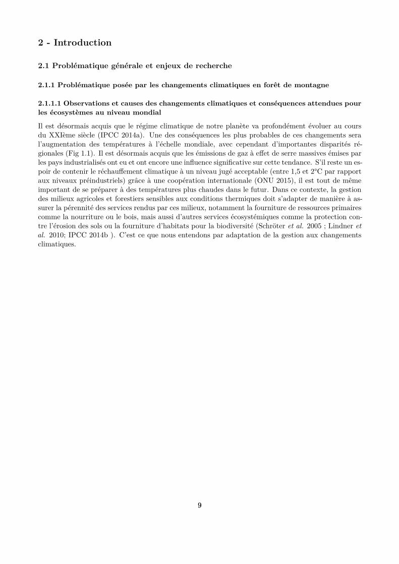
Il est désormais acquis que le régime climatique de notre planète va profondément évoluer au coursdu XXIème siècle (IPCC 2014a). Une des conséquences les plus probables de ces changements seral’augmentation des températures à l’échelle mondiale, avec cependant d’importantes disparités ré-gionales (Fig 1.1). Il est désormais acquis que les émissions de gaz à efet de serre massives émises parles pays industrialisés ont eu et ont encore une inluence signiicative sur cette tendance. S’il reste un es-poir de contenir le réchaufement climatique à un niveau jugé acceptable (entre 1,5 et 2°C par rapportaux niveaux préindustriels) grâce à une coopération internationale (ONU 2015), il est tout de mêmeimportant de se préparer à des températures plus chaudes dans le futur. Dans ce contexte, la gestiondes milieux agricoles et forestiers sensibles aux conditions thermiques doit s’adapter de manière à as-surer la pérennité des services rendus par ces milieux, notamment la fourniture de ressources primairescomme la nourriture ou le bois, mais aussi d’autres services écosystémiques comme la protection con-tre l’érosion des sols ou la fourniture d’habitats pour la biodiversité (Schröter et al. 2005 ; Lindner etal. 2010; IPCC 2014b ). C’est ce que nous entendons par adaptation de la gestion aux changementsclimatiques.
99
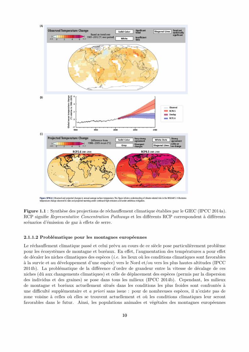
Figure 1.1 : Synthèse des projections de réchaufement climatique établies par le GIEC (IPCC 2014a).RCP signiie Representative Concentration Pathways et les diférents RCP correspondent à diférentsscénarios d’émission de gaz à efets de serre.
2.1.1.2 Problématique pour les montagnes européennes
Le réchaufement climatique passé et celui prévu au cours de ce siècle pose particulièrement problèmepour les écosystèmes de montagne et boréaux. En efet, l’augmentation des températures a pour efetde décaler les niches climatiques des espèces (i.e. les lieux où les conditions climatiques sont favorablesà la survie et au développement d’une espèce) vers le Nord et/ou vers les plus hautes altitudes (IPCC2014b). La problématique de la diférence d’ordre de grandeur entre la vitesse de décalage de cesniches (dû aux changements climatiques) et celle de déplacement des espèces (permis par la dispersiondes individus et des graines) se pose dans tous les milieux (IPCC 2014b). Cependant, les milieuxde montagne et boréaux actuellement situés dans les conditions les plus froides sont confrontés àune diiculté supplémentaire et a priori sans issue : pour de nombreuses espèces, il n’existe pas dezone voisine à celles où elles se trouvent actuellement et où les conditions climatiques leur serontfavorables dans le futur. Ainsi, les populations animales et végétales des montagnes européennes
1010
devraient être particulièrement impactées par le réchaufement climatique, avec un risque importantde voir des espèces disparaître (Thuiller et al. 2005) (Fig. 1.2). De plus, les modèles climatiquesactuels prévoient un réchaufement plus accentué dans les milieux de montagne, ce qui aggraverait cephénomène (Lindner et al. 2010).
Figure 1.2 : Projection d’évolution de la richesse spéciique en Europe. Le gradient de rouge indiqueune baisse de la richesse d’autant plus importante que la couleur est vive. Inversement, le gradient degris indique une hausse de la richesse d’autant plus important que la couleur est vive (Thuiller et al.2005).
2.1.1.3 Cas des hêtraies-sapinières-pessières gérées
Les hêtraies-sapinières-pessières (i.e. les forêts majoritairement composées d’épicéas (Picea abies (L.)Karst.), de sapins (Abies alba Mill.) et/ou de hêtres (Fagus sylvatica L.)) sont des forêts courantesdans les zones de montagne humides et fraîches d’Europe. Elles sont très souvent exploitées pour leurbois, et donc gérées de manière à obtenir une production durable de ce matériau. L’économie généréepar cette ressource explique le grand intérêt de recherche porté sur ces forêts. De nombreuses études
1111

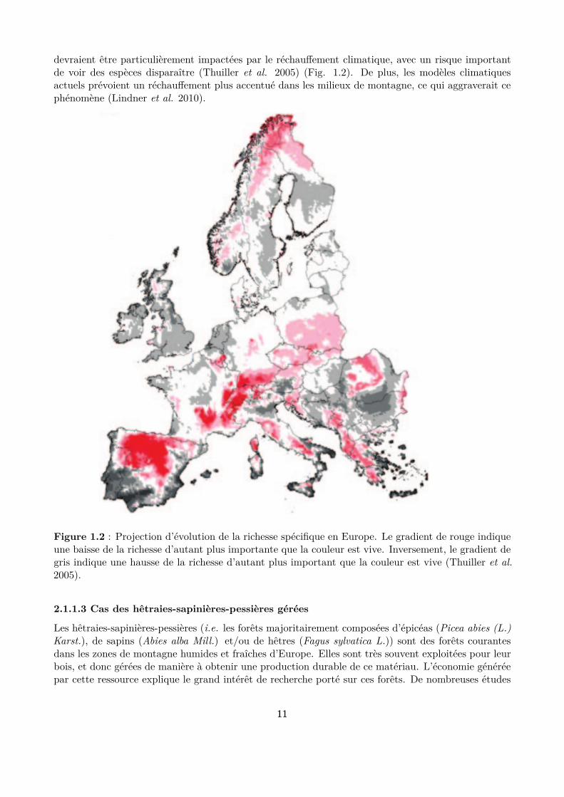
s’intéressent ainsi aux impacts des changements climatiques sur ces forêts, notamment en mesurant ledécalage de la distribution des espèces vers les hautes altitudes (Lenoir et al. 2008, 2009; Rabasa et al.2013), en étudiant les changements de composition en espèce des peuplements (Carcaillet & Muller2005; Pinto & Gégout 2005; Bolte et al. 2009; Peringer et al. 2013; Tinner et al. 2013; Schwörer,Henne & Tinner 2014) ou encore en modélisant la distribution géographique future des aires favorablesà ces espèces (Piedallu et al. 2009; Snell et al. 2014). Ces études montrent que les changementsclimatiques prévus devraient avoir un impact sensible sur la distribution de ces trois espèces (Piedalluet al. 2009) (Fig. 1.3) et sur la dynamique des forêts (Keenan 2015), et en conséquence égalementsur les diférents services rendus par ces écosystèmes, comme la production de bois, la conservation dela biodiversité ou la protection contre les chutes de bloc (Elkin et al. 2013). Cependant, les facteursclimatiques interagissent souvent avec d’autres facteurs écologiques ou anthropiques. La multiplicité etles interactions de ces facteurs brouillent souvent fortement les réponses de la dynamique des espècesaux variables climatiques et conduisent parfois à des résultats inattendus. Par exemple, la croissancedu hêtre a augmenté en réponse au réchaufement climatique en zone méditerranéenne, alors que cetteespèce, qui afectionne plutôt les conditions tempérées et humides, est considérée comme menacéedans ces milieux secs (Tegel et al. 2014). Il reste donc encore de grandes incertitudes sur la manièredont ces trois espèces vont s’adapter aux futures conditions climatiques et donc sur comment leshêtraies-sapinières-pessières vont évoluer (Lindner et al. 2014).
1212
Figure 1.3 : Évolution des surfaces en France actuellement forestières potentiellement favorables à ladistribution de l’épicéa , du sapin, du hêtre et du chêne sessile à l’horizon 2100, selon 2 scénarios dechangement climatique (A2 et B2, anciennes notations des scénarios du GIEC) (Piedallu et al. 2009).
2.1.2 Démographie forestière
2.1.2.1 Les diférents processus démographiques
Dans cette thèse, nous nous intéressons à la dynamique des peuplements forestiers gérés dans un con-texte de changement climatique. Trois grands processus démographiques sont généralement distinguéspour décrire la dynamique forestière : la croissance des arbres, la régénération naturelle (comprenantla production, la dispersion et la germination des graines, puis la croissance et la survie des semisjusqu’au stade adulte) et la mortalité des arbres. Il est pertinent de distinguer ces processus car cha-cun répond à sa manière aux diférents facteurs écologiques. Dans cette thèse, nous nous sommesfocalisés sur les processus de croissance et de régénération. En efet, la mortalité des arbres dansces forêts gérées est très souvent devancée par les opérations de récolte, ce qui à la fois raréie forte-ment des données d’observation sur ce processus et rend marginal son efet sur la dynamique de ces
1313
peuplements.
2.1.2.2 Les facteurs écologiques inluençant la démographie forestière
Les facteurs écologiques inluençant la démographie des forêts sont multiples. De plus, ils ne semanifestent pas avec la même intensité selon les échelles spatiale et temporelle considérées. Parexemple, il est capital de tenir compte de la variabilité journalière de la température pour étudierla physiologie des arbres (croissance des diférents organes, stockage de réserves, …) (Deckmyn etal. 2008), tandis que la démographie à long terme des peuplements dépend plutôt de la variabilitésaisonnière et inter-annuelle du climat (Fontes et al. 2010; Carrer, Motta & Nola 2012). L’objetd’étude de cette thèse étant la dynamique des peuplements forestiers à long terme (environ un siècle),nous nous focaliserons donc sur les facteurs pertinents à ces échelles temporelle et spatiale.
Pour mieux appréhender ces facteurs, il est utile de les regrouper par catégories. Nous avons utiliséquatre catégories : les facteurs abiotiques (inluence du non-vivant), les facteurs biotiques endogènes(interactions entre les arbres), les facteurs biotiques exogènes (inluence du vivant hors humains et horsarbres) et les facteurs anthropiques (inluence des humains). Les facteurs climatiques font partie desfacteurs abiotiques. Tous ces facteurs ont leurs efets propres mais également des efets en interactionavec les autres facteurs. Dans le descriptif qui suit, nous détaillerons les facteurs importants dechacune de ces quatre catégories et nous donnerons quelques éléments sur les interactions avec lesfacteurs climatiques qui nous intéressent particulièrement ici (température et précipitations).
2.1.2.2.1 Inluence des facteurs abiotiques
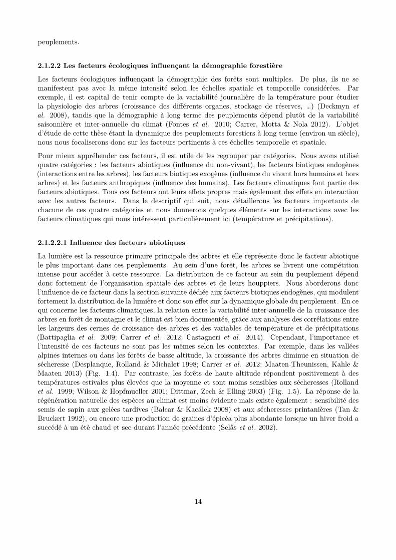
La lumière est la ressource primaire principale des arbres et elle représente donc le facteur abiotiquele plus important dans ces peuplements. Au sein d’une forêt, les arbres se livrent une compétitionintense pour accéder à cette ressource. La distribution de ce facteur au sein du peuplement dépenddonc fortement de l’organisation spatiale des arbres et de leurs houppiers. Nous aborderons doncl’inluence de ce facteur dans la section suivante dédiée aux facteurs biotiques endogènes, qui modulentfortement la distribution de la lumière et donc son efet sur la dynamique globale du peuplement. En cequi concerne les facteurs climatiques, la relation entre la variabilité inter-annuelle de la croissance desarbres en forêt de montagne et le climat est bien documentée, grâce aux analyses des corrélations entreles largeurs des cernes de croissance des arbres et des variables de température et de précipitations(Battipaglia et al. 2009; Carrer et al. 2012; Castagneri et al. 2014). Cependant, l’importance etl’intensité de ces facteurs ne sont pas les mêmes selon les contextes. Par exemple, dans les valléesalpines internes ou dans les forêts de basse altitude, la croissance des arbres diminue en situation desécheresse (Desplanque, Rolland & Michalet 1998; Carrer et al. 2012; Maaten-Theunissen, Kahle &Maaten 2013) (Fig. 1.4). Par contraste, les forêts de haute altitude répondent positivement à destempératures estivales plus élevées que la moyenne et sont moins sensibles aux sécheresses (Rollandet al. 1999; Wilson & Hopfmueller 2001; Dittmar, Zech & Elling 2003) (Fig. 1.5). La réponse de larégénération naturelle des espèces au climat est moins évidente mais existe également : sensibilité dessemis de sapin aux gelées tardives (Balcar & Kacálek 2008) et aux sécheresses printanières (Tan &Bruckert 1992), ou encore une production de graines d’épicéa plus abondante lorsque un hiver froid asuccédé à un été chaud et sec durant l’année précédente (Selås et al. 2002).
1414
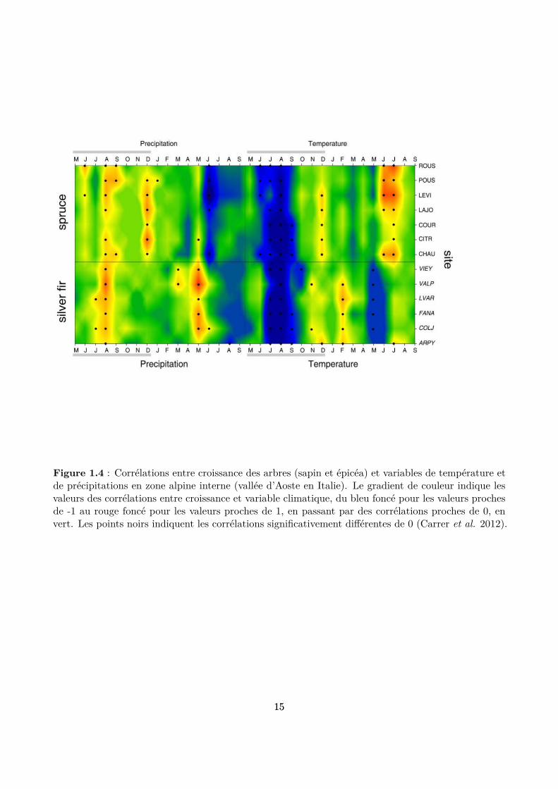
Figure 1.4 : Corrélations entre croissance des arbres (sapin et épicéa) et variables de température etde précipitations en zone alpine interne (vallée d’Aoste en Italie). Le gradient de couleur indique lesvaleurs des corrélations entre croissance et variable climatique, du bleu foncé pour les valeurs prochesde -1 au rouge foncé pour les valeurs proches de 1, en passant par des corrélations proches de 0, envert. Les points noirs indiquent les corrélations signiicativement diférentes de 0 (Carrer et al. 2012).
1515
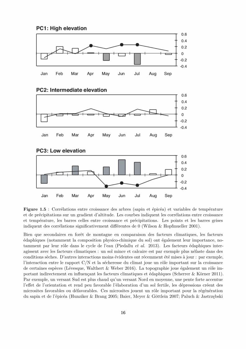
Figure 1.5 : Corrélations entre croissance des arbres (sapin et épicéa) et variables de températureet de précipitations sur un gradient d’altitude. Les courbes indiquent les corrélations entre croissanceet température, les barres celles entre croissance et précipitations. Les points et les barres grisesindiquent des corrélations signiicativement diférentes de 0 (Wilson & Hopfmueller 2001).
Bien que secondaires en forêt de montagne en comparaison des facteurs climatiques, les facteursédaphiques (notamment la composition physico-chimique du sol) ont également leur importance, no-tamment par leur rôle dans le cycle de l’eau (Piedallu et al. 2013). Les facteurs édaphiques inter-agissent avec les facteurs climatiques : un sol mince et calcaire est par exemple plus néfaste dans desconditions sèches. D’autres interactions moins évidentes ont récemment été mises à jour : par exemple,l’interaction entre le rapport C/N et la sécheresse du climat joue un rôle important sur la croissancede certaines espèces (Lévesque, Walthert & Weber 2016). La topographie joue également un rôle im-portant indirectement en inluençant les facteurs climatiques et édaphiques (Scherrer & Körner 2011).Par exemple, un versant Sud est plus chaud qu’un versant Nord en moyenne, une pente forte accentuel’efet de l’orientation et rend peu favorable l’élaboration d’un sol fertile, les dépressions créent desmicrosites favorables ou défavorables. Ces microsites jouent un rôle important pour la régénérationdu sapin et de l’épicéa (Hunziker & Brang 2005; Baier, Meyer & Göttlein 2007; Paluch & Jastrzębski
1616
2013) (Fig. 1.6).
Figure 1.6 : Exemple de microsite favorable à l’installation des semis d’épicéa.
2.1.2.2.2 Inluence des facteurs biotiques endogènes
Des variables mesurées à l’échelle du peuplement (telles que la densité en arbres, la mixité des espèceset la diversité des tailles) sont souvent utilisées pour quantiier ces facteurs. Elles rendent compteindirectement des interactions (compétition ou facilitation) existant entre les arbres pour les ressources,notamment pour la lumière qui est la ressource clé dans ces peuplements. Les peuplements des hêtraies-sapinières-pessières ont la particularité de présenter généralement une structure inéquienne (i.e unmélange d’arbres de tous âges, quelle que soit l’échelle spatiale considérée) et une mixité en espèces.Ils sont dits “irréguliers” et “mélangés”. La mixité des espèces et la diversité des tailles a une inluencesur la démographie de ces peuplements, en particulier sur la croissance des arbres : la production d’unpeuplement augmente généralement avec la richesse en espèces (Morin et al. 2011) ; une plus grandehétérogénéité de taille des arbres, en modiiant la distribution de lumière dans le peuplement, a selonles études un efet négatif (Bourdier et al. 2016) (Fig. 1.7) ou positif (Dănescu, Albrecht & Bauhus
1717
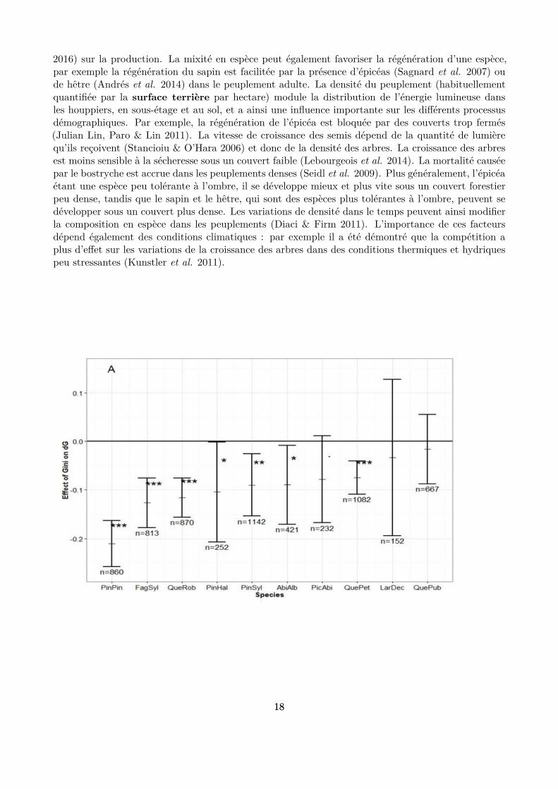
2016) sur la production. La mixité en espèce peut également favoriser la régénération d’une espèce,par exemple la régénération du sapin est facilitée par la présence d’épicéas (Sagnard et al. 2007) oude hêtre (Andrés et al. 2014) dans le peuplement adulte. La densité du peuplement (habituellementquantiiée par la surface terrière par hectare) module la distribution de l’énergie lumineuse dansles houppiers, en sous-étage et au sol, et a ainsi une inluence importante sur les diférents processusdémographiques. Par exemple, la régénération de l’épicéa est bloquée par des couverts trop fermés(Julian Lin, Paro & Lin 2011). La vitesse de croissance des semis dépend de la quantité de lumièrequ’ils reçoivent (Stancioiu & O’Hara 2006) et donc de la densité des arbres. La croissance des arbresest moins sensible à la sécheresse sous un couvert faible (Lebourgeois et al. 2014). La mortalité causéepar le bostryche est accrue dans les peuplements denses (Seidl et al. 2009). Plus généralement, l’épicéaétant une espèce peu tolérante à l’ombre, il se développe mieux et plus vite sous un couvert forestierpeu dense, tandis que le sapin et le hêtre, qui sont des espèces plus tolérantes à l’ombre, peuvent sedévelopper sous un couvert plus dense. Les variations de densité dans le temps peuvent ainsi modiierla composition en espèce dans les peuplements (Diaci & Firm 2011). L’importance de ces facteursdépend également des conditions climatiques : par exemple il a été démontré que la compétition aplus d’efet sur les variations de la croissance des arbres dans des conditions thermiques et hydriquespeu stressantes (Kunstler et al. 2011).
1818
Figure 1.7 : Efet de la diversité en taille (quantiiée par le coeicient de Gini, la diversité étantd’autant plus grande que ce coeicient est élevé) sur la production (accroissement en surface terrière)d’un peuplement. En abscisse, les codes indiquent les espèces (FagSyl pour le hêtre, PicAbi pourl’épicéa et AbiAlb pour le sapin pour ce qui concerne les espèces étudiées dans cette thèse). Lesvaleurs négatives en ordonnée indiquent un efet négatif de l’hétérogénéité en taille sur la production(Bourdier et al. 2016).
2.1.2.2.3 Inluence des facteurs biotiques exogènes
Logiquement, les facteurs biotiques exogènes bien documentés concernent ceux qui ont des efetsnégatifs. Dans les hêtraies-sapinières-pessières, les plus inluents sont les grands herbivores forestiers,comme le cerf élaphe (Cervus elaphus) , le chevreuil (Capreolus capreolus) ou le sanglier (Sus scrofa),et les insectes ravageurs, principalement le bostryche typographe (Ips typographus). Les premiers fontprincipalement des ravages en broutant les semis (particulièrement ceux de sapin) (Motta 1996) etle bostryche provoque régulièrement la mort d’un nombre important d’épicéas dans certaines forêts(Pasztor et al. 2014). Si les inluences directes de ces ravageurs ont été intensivement étudiées, leursinteractions avec les facteurs climatiques sont beaucoup plus complexes et restent encore largementméconnues, malgré quelques études récentes sur ce sujet (Seidl et al. 2008; Cailleret, Heurich &Bugmann 2014).
2.1.2.2.4 Inluence des facteurs anthropiques
Les facteurs anthropiques ont un rôle important dans ces forêts. Les hêtraies-sapinières-pessières sonten efet très souvent gérées de longue date, et la structure et la composition des peuplements ont doncsouvent été inluencées par les interventions humaines. La gestion irrégulière, typiquement appliquéedans ces peuplements, est détaillée plus loin (cf. section 1.3). Plus concrètement, les coupes forestièresont de longue date favorisé indirectement la croissance et la régénération de l’épicéa, au détriment dusapin et du hêtre, pour des raisons économiques (meilleure qualité du bois). En pratique, cela consistepar exemple à maintenir des densités basses ou à créer des trouées (Grassi et al. 2004; Gauquelin& Courbaud 2006 ). Les plantations et les travaux forestiers dans les stades juvéniles sont d’autresexemples d’efets directs de la gestion forestière sur la démographie des espèces qui viennent régulerl’efet des autres facteurs (et notamment le climat). Il est donc important de tenir compte de lagestion appliquée au peuplement pour analyser sa dynamique passée et actuelle (Diaci & Firm 2011)(Fig. 1.8).
1919
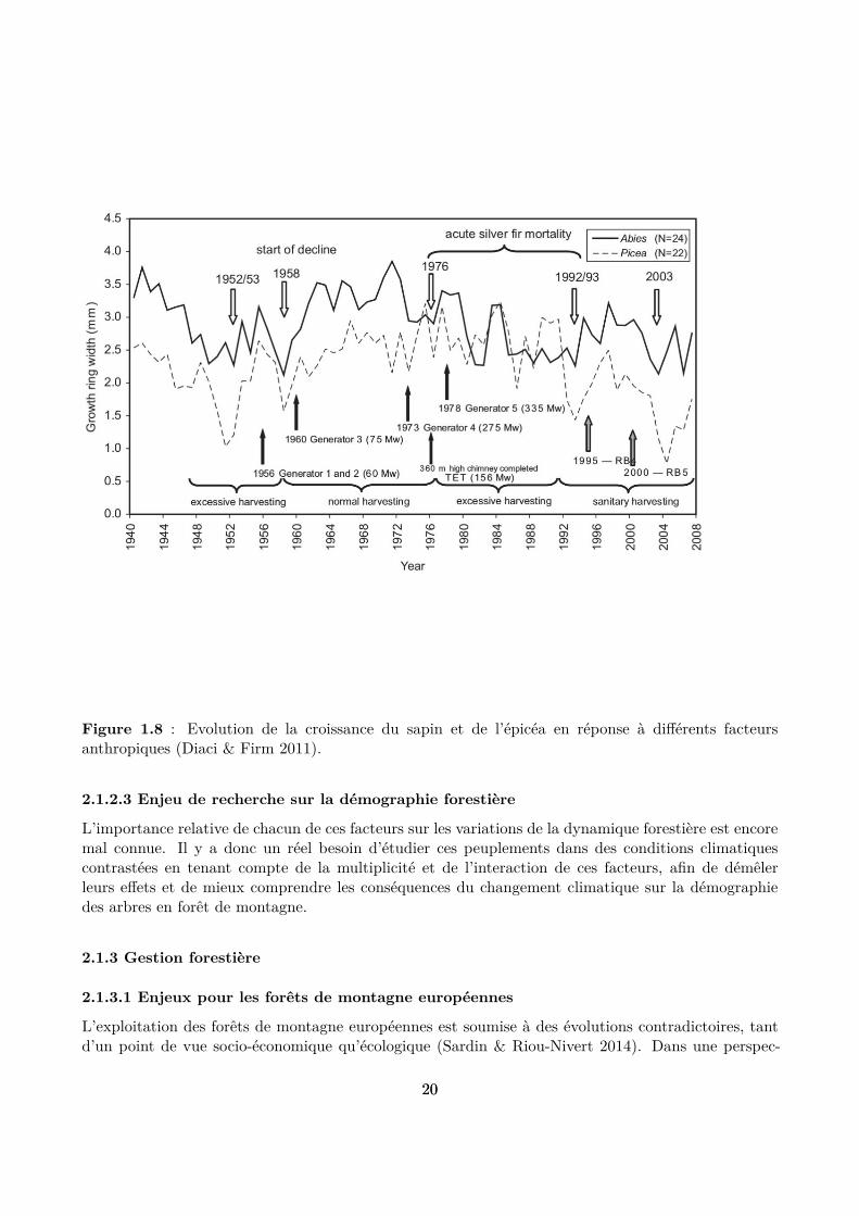
Figure 1.8 : Evolution de la croissance du sapin et de l’épicéa en réponse à diférents facteursanthropiques (Diaci & Firm 2011).
2.1.2.3 Enjeu de recherche sur la démographie forestière
L’importance relative de chacun de ces facteurs sur les variations de la dynamique forestière est encoremal connue. Il y a donc un réel besoin d’étudier ces peuplements dans des conditions climatiquescontrastées en tenant compte de la multiplicité et de l’interaction de ces facteurs, ain de démêlerleurs efets et de mieux comprendre les conséquences du changement climatique sur la démographiedes arbres en forêt de montagne.
2.1.3 Gestion forestière
2.1.3.1 Enjeux pour les forêts de montagne européennes
L’exploitation des forêts de montagne européennes est soumise à des évolutions contradictoires, tantd’un point de vue socio-économique qu’écologique (Sardin & Riou-Nivert 2014). Dans une perspec-
2020
tive de développement durable, l’exploitation du bois dans les forêts locales présente de nombreuxavantages (circuits courts limitant les émissions de polluants atmosphériques, utilisation d’une énergierenouvelable, stockage du carbone), mais, en pratique, le manque de valorisation économique des bois,les diicultés d’exploitation des peuplements de montagne et la déprise agricole ont plutôt conduit àune sous-exploitation de ces forêts (Constantin & Vauterin 1998). D’un point de vue écologique, dansun contexte de réchaufement climatique, l’exploitation forestière devrait bénéicier de l’augmentationattendue de la croissance des arbres en réponse à des températures plus élevées et donc moins limitantesen montagne (Rolland, Petitcolas & Michalet 1998; Bolli, Rigling & Bugmann 2007). Cependant, lesgestionnaires craignent également une augmentation de la mortalité des arbres due à une occurrenceaccrue des sécheresses et des tempêtes, une augmentation de la compétition avec d’autres espèces végé-tales plus thermophiles et plus compétitrices ou encore une pression accrue des parasites (notammentles grands ongulés et les insectes ravageurs) (Hlásny et al. 2011; Lindner et al. 2014; Keenan 2015).Tous ces éléments soulèvent des questions importantes pour planiier la sylviculture à moyen et longterme.
2.1.3.2 Gestion de peuplements inéquiens
La gestion forestière appliquée dans ces peuplements est dite irrégulière, par opposition à la gestionrégulière propre aux peuplements équiens. En pratique, la gestion irrégulière consiste à combiner desopérations de récolte et d’amélioration à chaque passage du peuplement en coupe, et il n’existe pasde coupe rase dans ce type de gestion. Les arbres à couper sont sélectionnés individuellement oupar petits groupes par les gestionnaires, selon diférents critères hiérarchisés de manière à optimiserla production de bois et le renouvellement des peuplements (récolte des arbres arrivés à maturité,suppression d’un arbre en mauvaise santé ou gênant un voisin de meilleure qualité, mise en lumière desemis) (Schütz 1997). Ce type de gestion permet de prendre en considération les diférents servicesécosystémiques forestiers (comme la production de bois et la protection contre la chute de blocsrocheux) et présente de nombreux avantages d’un point de vue écologique (notamment le mélangede plusieurs espèces d’arbres et le maintien permanent d’un couvert forestier). Cependant, ce typede gestion est complexe à mettre en oeuvre car il présente de nombreuses subtilités qui permettentdes variations à l’inini des interventions. Les guides de sylviculture comme ceux rédigés par l’ONFfournissent des renseignements précieux pour déinir des modalités de gestion adaptées aux diférentesconditions stationnelles (Gauquelin & Courbaud 2006) mais donnent encore peu d’éléments concretssur l’adaptation de ce type de gestion au changement climatique.
2.1.3.3 Adaptation de la sylviculture au changement climatique
La littérature scientiique concernant l’adaptation de la sylviculture au changement climatique s’estconsidérablement enrichie au cours des dix dernières années (Fig. 1.9). Plusieurs éléments ont été iden-tiiés comme importants à prendre en compte pour aborder ce sujet : évaluer d’abord la vulnérabilitédes peuplements ; échanger avec les gestionnaires ; tenir compte des diférentes sources d’incertitude ;ne pas engager d’actions irréversibles (Courbaud et al. 2010; Seidl, Rammer & Lexer 2011a; Keenan2015). Le maintien des services écosystémiques forestiers des peuplements est un élément supplémen-taire à prendre en compte (Elkin et al. 2013). Les études publiées sur l’adaptation de la sylviculturedes hêtraies-sapinières-pessières de montagne au changement climatique déclinent toutes ou une par-tie de ces recommandations générales sur des cas d’étude, par exemple sur les forêts autrichiennes(Seidl et al. 2011a; Seidl, Rammer & Lexer 2011b), sur les forêts Suisse (Elkin et al. 2013, 2015) ouencore en Roumanie (Bouriaud et al. 2014).
Plusieurs pistes d’adaptation reviennent couramment : favoriser le mélange des espèces, particulière-ment dans les peuplements riches en épicéas à cause de la sensibilité présumée de cette espèce au
2121
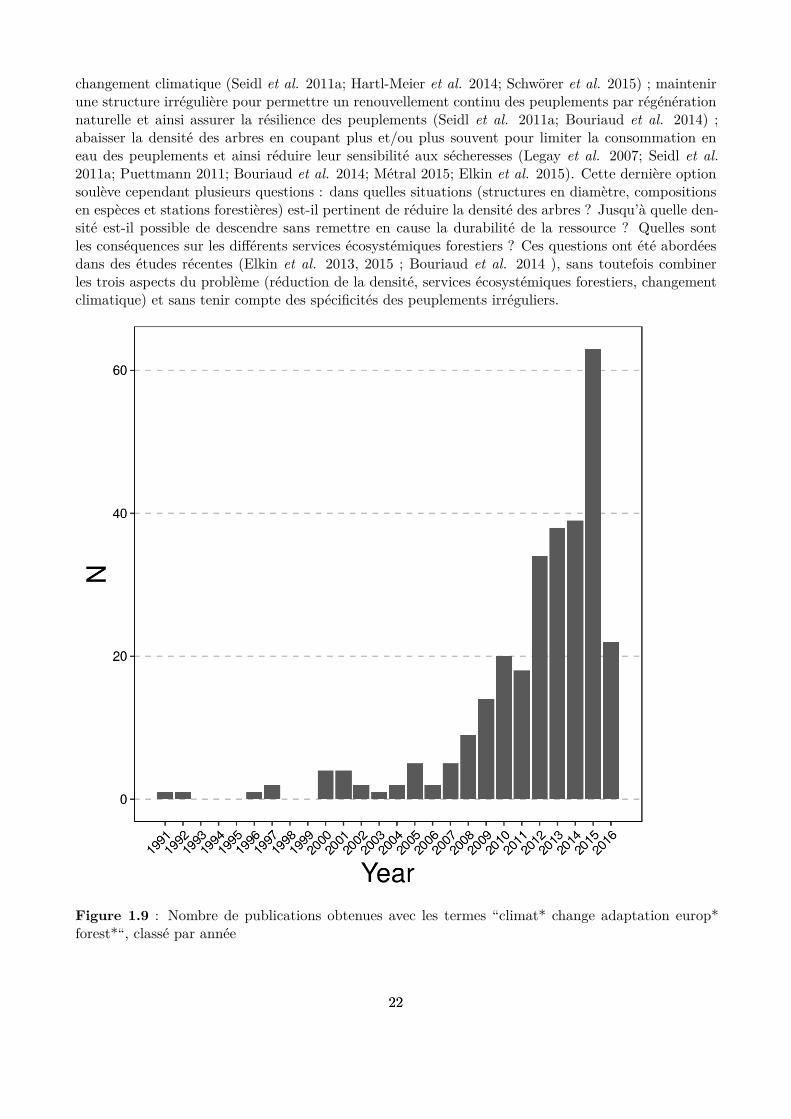
changement climatique (Seidl et al. 2011a; Hartl-Meier et al. 2014; Schwörer et al. 2015) ; maintenirune structure irrégulière pour permettre un renouvellement continu des peuplements par régénérationnaturelle et ainsi assurer la résilience des peuplements (Seidl et al. 2011a; Bouriaud et al. 2014) ;abaisser la densité des arbres en coupant plus et/ou plus souvent pour limiter la consommation eneau des peuplements et ainsi réduire leur sensibilité aux sécheresses (Legay et al. 2007; Seidl et al.2011a; Puettmann 2011; Bouriaud et al. 2014; Métral 2015; Elkin et al. 2015). Cette dernière optionsoulève cependant plusieurs questions : dans quelles situations (structures en diamètre, compositionsen espèces et stations forestières) est-il pertinent de réduire la densité des arbres ? Jusqu’à quelle den-sité est-il possible de descendre sans remettre en cause la durabilité de la ressource ? Quelles sontles conséquences sur les diférents services écosystémiques forestiers ? Ces questions ont été abordéesdans des études récentes (Elkin et al. 2013, 2015 ; Bouriaud et al. 2014 ), sans toutefois combinerles trois aspects du problème (réduction de la densité, services écosystémiques forestiers, changementclimatique) et sans tenir compte des spéciicités des peuplements irréguliers.
Figure 1.9 : Nombre de publications obtenues avec les termes “climat* change adaptation europ*forest*“, classé par année
2222
2.1.3.4 Enjeu de recherche sur la gestion irrégulière
Il est intéressant de noter à cet égard qu’il y a très peu d’études s’intéressant à l’adaptation de lagestion irrégulière au changement climatique. Trois raisons principales peuvent expliquer cette lacune.D’abord, les peuplements irréguliers sont largement minoritaires et souvent moins productifs (caressentiellement situés en zone montagneuse) que les peuplements réguliers, donc moins intéressantsd’un point de vue économique et social. D’autre part, du fait de leur structure inéquienne et deleur composition mélangée, ils sont reconnus comme étant plus résistants et plus résilients aux aléasclimatiques (O’Hara 2006 ; DeClerck, Barbour & Sawyer 2006 ; Cordonnier et al. 2008; Jactel et al.2009; Seidl et al. 2011a; Puettmann 2011). Enin, la gestion irrégulière est par nature une gestionadaptative car les diférents processus démographiques sont modulés à chaque intervention au lieud’être séparés dans le temps. Elle s’ajuste régulièrement à l’état et à la composition des peuplements,et pourrait donc nécessiter moins d’adaptations spéciiques au changement climatique (Métral 2015).Cependant, la mise en évidence de la vulnérabilité des espèces de montagne à un climat plus chaud,les nombreuses possibilités d’adaptation de ce type de gestion et les questions posées par la réductionde la densité justiient que la recherche s’y intéresse de plus près.
2.2 Données et outils d’analyse à disposition
2.2.1 Les données historiques de gestion
La gestion irrégulière des forêts impose d’avoir un suivi des opérations forestières menées dans lespeuplements. Ces suivis ont souvent été conservés sur de longues périodes de temps et constituent unesource de données potentiellement intéressante pour les chercheurs. A partir de plusieurs sources, cesarchives ont été récupérées pour un nombre important de peuplements. Ce jeu de données constitue lamatière première de ce travail de thèse. La partie 1 de ce manuscrit détaille la nature de ces donnéeset la façon dont elles ont été collectées.
2.2.2 La modélisation
En écologie forestière comme dans bien d’autres domaines scientiiques s’intéressant à des systèmescomplexes, il est aujourd’hui courant de recourir à la modélisation. Le principe général de cettemodélisation consiste à représenter de manière plus ou moins simpliiée la dynamique du systèmepar des équations mathématiques, contenant des paramètres et des variables. La décompositiondu fonctionnement global en processus simples permet de faciliter l’analyse et la compréhension dusystème, et de projeter son évolution.
2.2.3 La modélisation de la dynamique forestière
2.2.3.1 Considérations générales
Pour étudier la dynamique forestière, l’approche par modélisation se justiie pour plusieurs raisons :
• la dynamique de ces forêts s’étend sur de longues durées, ce qui rend les expérimentations insitu compliquées et coûteuses ;
• de multiples facteurs écologiques interagissent entre eux, ce qui fait des peuplements forestiersdes systèmes complexes ;
• les modèles de dynamique forestière peuvent ensuite être associés à d’autres modèles, commepar exemple des modèles d’évolution du climat, pour aborder des questions plus globales.
2323
Une grande variété de modèles de dynamique forestière ont été développés au cours des vingt dernièresannées (Fontes et al. 2010). Le manque de connaissances sur les processus démographiques et lafaible disponibilité des données font que la formalisation et la calibration de certaines relations entredémographie forestière et facteurs écologiques sont diiciles voire parfois impossibles à réaliser. Il estcompréhensible dès lors que les modélisateurs se sont attachés à d’abord intégrer dans les modèlesles facteurs les plus inluents pour lesquels il existe des données de terrain permettant de calibrer lesdiférents processus.
2.2.3.2 Le modèle Samsara2
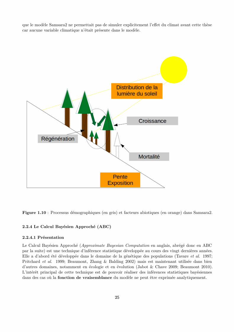
Samsara2 est un modèle de dynamique forestière individu-centré (i.e. l’élément de base du modèle estl’arbre) et spatialement explicite (i.e. la position de chaque arbre est déinie dans les 3 dimensions)(Courbaud et al. 2015) (Fig. 1.10). De plus, ce modèle intègre une représentation spatiale du substrat,caractérisée par un plan incliné avec une orientation géographique. L’originalité de ce modèle résidedans la représentation explicite de la distribution de la lumière au-dessus et au-dessous du couvertdes arbres, en tenant compte du cheminement du soleil au cours d’une journée et d’une année, de latopographie et de l’interception des rayons lumineux par les houppiers des arbres (Courbaud, Coligny& Cordonnier 2003) (Fig. 1.10).
Ce modèle a été spéciiquement conçu pour simuler la dynamique des hêtraies-sapinières-pessièresde montagne à une échelle géographique ine (peuplement, i.e. 1-10 ha). Les diférents processusdémographiques (croissance, régénération et mortalité) sont représentés à l’échelle de l’arbre à partirde la lumière parvenant sur le peuplement. Le modèle calcule la proportion de lumière interceptée parle houppier de chaque arbre adulte (DBH > 7.5 cm) et la croissance d’un arbre donné est d’autant plusgrande que son houppier intercepte plus de lumière. La survie et la croissance des semis dépendentquant à elles des conditions lumineuses au sol, c’est à dire de la part de lumière qui parvient au solaprès avoir franchi les houppiers des arbres adultes. La croissance des semis est d’autant plus rapideque la lumière au sol est abondante. La fonction de réponse de la survie des semis à la lumière présenteune forme en cloche, avec un optimum pour une proportion de lumière aux alentours de 60% de pleinelumière. La mortalité des arbres adultes ne dépend pas directement de la lumière. La probabilité demourir chaque année pour un arbre donné dépend de sa taille (mortalité par sénescence : plus la tailleest grande, plus la probabilité de mourir est grande) et de la densité des arbres plus gros que lui dansson environnement proche (mortalité par compétition : plus la densité d’arbres adultes plus gros estgrande, plus la probabilité de mourir est grande).
Les dimensions de l’arbre (hauteur et taille du houppier) sont dérivées de son DBH par des équationsallométriques. Les équations démographiques et allométriques contiennent des paramètres dont lesvaleurs sont diférentes pour chaque espèce (21 par espèce). Ces paramètres ont été calibrés à partirde diférentes sources de données (données de terrain, bibliographie). Ces données de calibrationinitiale de Samsara2 sont spéciiques à chaque processus et n’ont donc pas permis de tenir comptede la covariance entre processus. Toutes les équations contiennent une part de stochasticité pourprendre en compte la variabilité individuelle constatée dans les données de calibration. Au coursd’une simulation de la dynamique d’un peuplement, les arbres sont donc en compétition les uns avecles autres pour la lumière et tous les processus démographiques interagissent au cours de la simulation,ce qui permet de prendre en compte de façon explicite les facteurs biotiques endogènes intervenantdans la dynamique de ces communautés forestières.
Ce modèle est utilisé pour former des étudiants et pour aider les gestionnaires forestiers concernéspar la sylviculture irrégulière. Il a également été utilisé dans un contexte de recherche pour testerdiférentes modalités de gestion irrégulière (Lafond et al. 2014). Il est important de mentionner ici
2424
que le modèle Samsara2 ne permettait pas de simuler explicitement l’efet du climat avant cette thèsecar aucune variable climatique n’était présente dans le modèle.
Figure 1.10 : Processus démographiques (en gris) et facteurs abiotiques (en orange) dans Samsara2.
2.2.4 Le Calcul Bayésien Approché (ABC)
2.2.4.1 Présentation
Le Calcul Bayésien Approché (Approximate Bayesian Computation en anglais, abrégé donc en ABCpar la suite) est une technique d’inférence statistique développée au cours des vingt dernières années.Elle a d’abord été développée dans le domaine de la génétique des populations (Tavare et al. 1997;Pritchard et al. 1999; Beaumont, Zhang & Balding 2002) mais est maintenant utilisée dans biend’autres domaines, notamment en écologie et en évolution (Jabot & Chave 2009; Beaumont 2010).L’intérêt principal de cette technique est de pouvoir réaliser des inférences statistiques bayésiennesdans des cas où la fonction de vraisemblance du modèle ne peut être exprimée analytiquement.
2525
2.2.4.2 Principe de fonctionnement
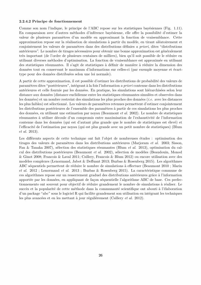
Comme son nom l’indique, le principe de l’ABC repose sur les statistiques bayésiennes (Fig. 1.11).En comparaison avec d’autres méthodes d’inférence bayésienne, elle ofre la possibilité d’estimer lavaleur de plusieurs paramètres d’un modèle en approximant la fonction de vraisemblance. Cetteapproximation repose sur la réalisation de simulations à partir du modèle, en tirant aléatoirement etconjointement les valeurs de paramètres dans des distributions déinies a priori, dites “distributionsantérieures”. Le nombre de tirages nécessaires pour obtenir une bonne approximation est généralementtrès important (de l’ordre de plusieurs centaines de milliers), bien qu’il soit possible de le réduire enutilisant diverses méthodes d’optimisation. La fonction de vraisemblance est approximée en utilisantdes statistiques résumantes. Il s’agit de statistiques à déinir de manière à réduire la dimension desdonnées tout en conservant le maximum d’informations sur celles-ci (par exemple moyenne et écart-type pour des données distribuées selon une loi normale).
A partir de cette approximation, il est possible d’estimer les distributions de probabilité des valeurs deparamètres dites “postérieures”, intégrant à la fois l’information a priori contenue dans les distributionsantérieures et celle fournie par les données. En pratique, les simulations sont hiérarchisées selon leurdistance aux données (distance euclidienne entre les statistiques résumantes simulées et observées dansles données) et un nombre restreint des simulations les plus proches des données (i.e. avec les distancesles plus faibles) est sélectionné. Les valeurs de paramètres retenues permettent d’estimer conjointementles distributions postérieures de l’ensemble des paramètres à partir de ces simulations les plus prochesdes données, en utilisant une estimation par noyau (Beaumont et al. 2002). Le nombre de statistiquesrésumantes à utiliser découle d’un compromis entre maximisation de l’exhaustivité de l’informationcontenue dans les données (qui est d’autant plus grande que le nombre de statistiques est élevé) etl’eicacité de l’estimation par noyau (qui est plus grande avec un petit nombre de statistiques) (Blumet al. 2013).
Les diférents aspects de cette technique ont fait l’objet de nombreuses études : optimisation destirages des valeurs de paramètres dans les distributions antérieures (Marjoram et al. 2003; Sisson,Fan & Tanaka 2007), sélection des statistiques résumantes (Blum et al. 2013), optimisation du cal-cul des distributions postérieures (Beaumont et al. 2002), sélection de modèles (Beaudouin, Monod& Ginot 2008; Francois & Laval 2011; Csillery, Francois & Blum 2012) ou encore utilisation avec desmodèles complexes (Lenormand, Jabot & Defuant 2013; Buzbas & Rosenberg 2015). Les algorithmesABC séquentiels permettent de réduire le nombre de simulations à efectuer (Beaumont 2010 ; Marinet al. 2012 ; Lenormand et al. 2013 ; Buzbas & Rosenberg 2015). La caractéristique commune deces algorithmes repose sur un resserrement graduel des distributions antérieures grâce à l’informationapportée par les données, en appliquant de façon séquentielle l’algorithme ABC de base. Ces perfec-tionnements ont souvent pour objectif de réduire grandement le nombre de simulations à réaliser. Lesuccès et la popularité de cette méthode dans la communauté scientiique ont abouti à l’élaborationd’un package “abc” sous le logiciel R qui facilite grandement son utilisation en intégrant les techniquesles plus avancées et en les mettant à jour régulièrement (Csillery et al. 2012).
2626
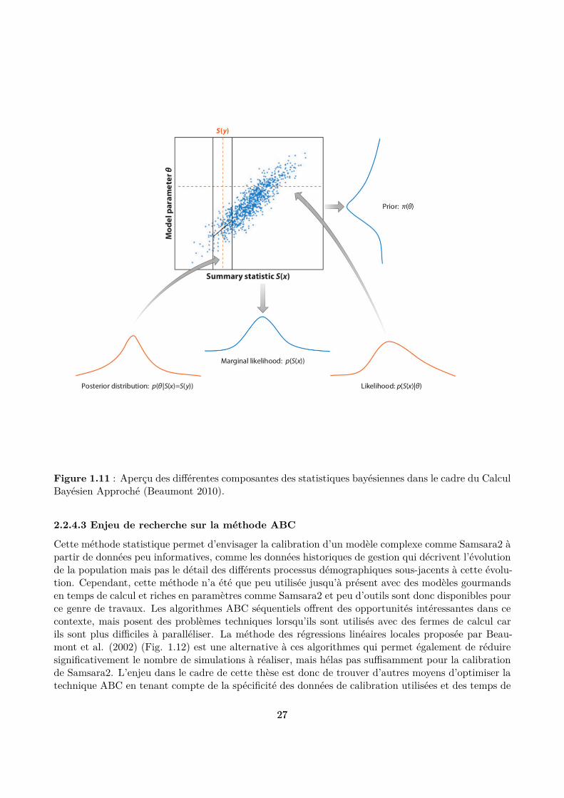
Figure 1.11 : Aperçu des diférentes composantes des statistiques bayésiennes dans le cadre du CalculBayésien Approché (Beaumont 2010).
2.2.4.3 Enjeu de recherche sur la méthode ABC
Cette méthode statistique permet d’envisager la calibration d’un modèle complexe comme Samsara2 àpartir de données peu informatives, comme les données historiques de gestion qui décrivent l’évolutionde la population mais pas le détail des diférents processus démographiques sous-jacents à cette évolu-tion. Cependant, cette méthode n’a été que peu utilisée jusqu’à présent avec des modèles gourmandsen temps de calcul et riches en paramètres comme Samsara2 et peu d’outils sont donc disponibles pource genre de travaux. Les algorithmes ABC séquentiels ofrent des opportunités intéressantes dans cecontexte, mais posent des problèmes techniques lorsqu’ils sont utilisés avec des fermes de calcul carils sont plus diiciles à paralléliser. La méthode des régressions linéaires locales proposée par Beau-mont et al. (2002) (Fig. 1.12) est une alternative à ces algorithmes qui permet également de réduiresigniicativement le nombre de simulations à réaliser, mais hélas pas suisamment pour la calibrationde Samsara2. L’enjeu dans le cadre de cette thèse est donc de trouver d’autres moyens d’optimiser latechnique ABC en tenant compte de la spéciicité des données de calibration utilisées et des temps de
2727
calcul importants pour simuler ces données avec le modèle Samsara2.
Figure 1.12 : Illustration du principe des régressions linéaires locales pour l’optimisation du calculdes distributions postérieures (Csillery et al. 2010).
2.2.5 La modélisation de la gestion forestière
2.2.5.1 Considérations générales
Dans les peuplements gérés (c’est à dire subissant des coupes régulières), intégrer les interventionshumaines dans les simulations à long terme de l’évolution des peuplements forestiers est essentiel.Voici une présentation succincte des algorithmes de coupe utilisés en couplage avec Samsara2 dans lecadre de cette thèse.
2.2.5.2 Algorithme NV
2828

Ce premier algorithme a été développé pour reproduire la gestion réellement appliquée dans les sim-ulations de la dynamique passée des peuplements. Il permet d’adapter les informations synthétiquesissues de documents de gestion (nombre (N) et volume (V) des arbres récoltés) à un modèle individu-centré comme Samsara2 (Lafond et al. 2012). Il considère ainsi d’une part la liste des arbres avecses attributs (DBH, Espèce), qui constitue le peuplement à éclaircir, et d’autre part les informationsN et V donnant des informations sur la coupe à appliquer. Le principe de l’algorithme est de couperexactement N arbres et de s’approcher le plus possible de V, en changeant itérativement les arbressélectionnés pour la coupe dans la liste d’arbres disponibles. Un nombre N d’arbres est sélectionnéaléatoirement en début de simulation, puis un arbre de la sélection est échangé avec un autre dans laliste d’arbres dans le peuplement à chaque itération, jusqu’à ce que le volume des arbres sélectionnésne puisse plus se rapprocher de V. Quelques rainements ont été ajoutés depuis la parution du pre-mier algorithme (Lafond et al. 2012) : sélectionner en priorité les arbres les plus gros dans la sélectioninitiale ; distinguer les résineux des feuillus ; fournir une distribution par classes de diamètre plutôtque N et V seulement.
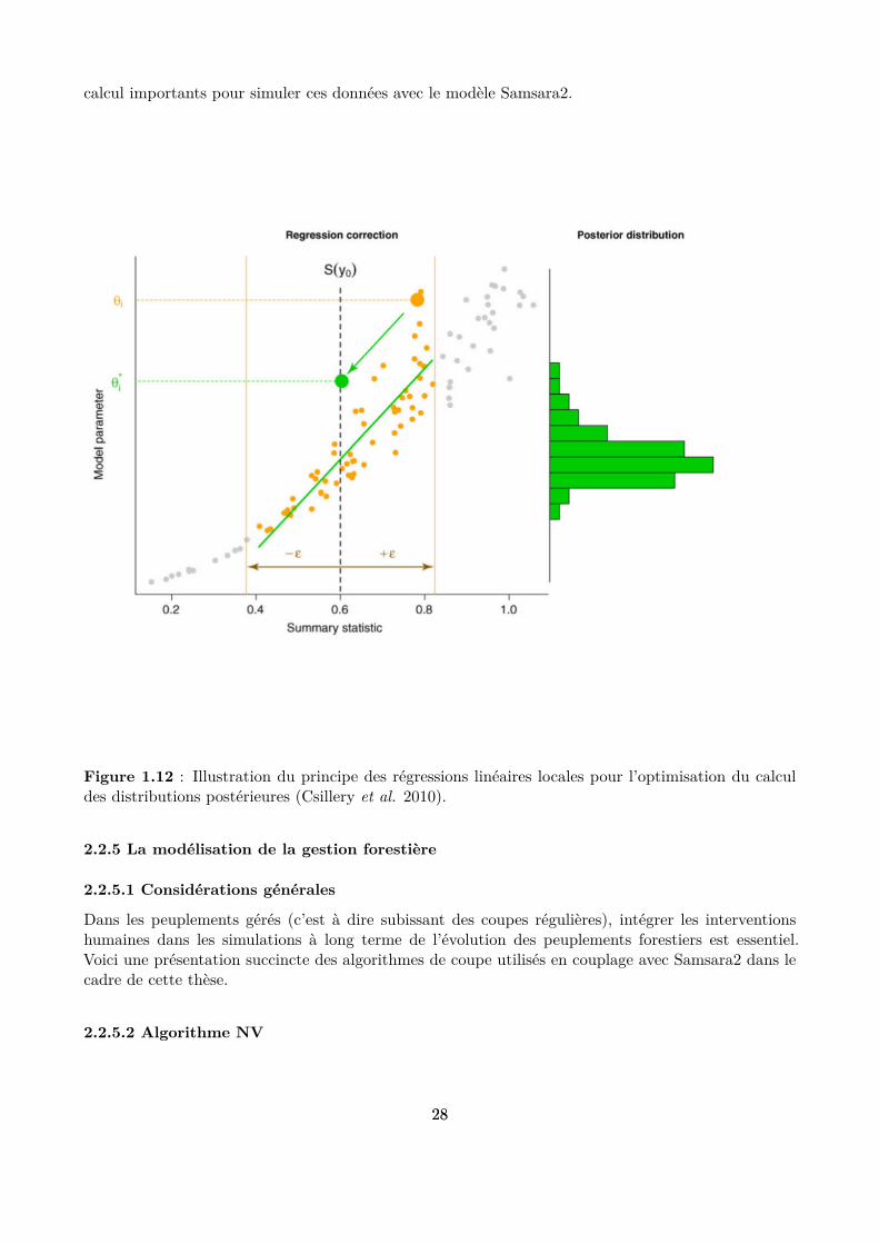
Cet algorithme a été testé sur des coupes pour lesquelles la distribution en classes de diamètre desarbres coupés était connue et il a été démontré qu’il permet de reproduire idèlement ces distributions(Lafond et al. 2012) (Fig. 1.13). Il a ainsi pu être utilisé pour valider le modèle Samsara2 à partir dedonnées historiques de gestion de la forêt de Queige (Courbaud et al. 2015).
2929
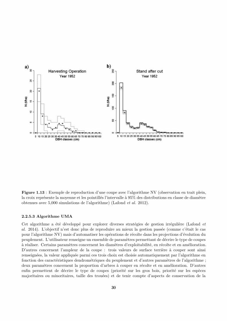
Figure 1.13 : Exemple de reproduction d’une coupe avec l’algorithme NV (observation en trait plein,la croix représente la moyenne et les pointillés l’intervalle à 95% des distributions en classe de diamètreobtenues avec 5,000 simulations de l’algorithme) (Lafond et al. 2012).
2.2.5.3 Algorithme UMA
Cet algorithme a été développé pour explorer diverses stratégies de gestion irrégulière (Lafond etal. 2014). L’objectif n’est donc plus de reproduire au mieux la gestion passée (comme c’était le caspour l’algorithme NV) mais d’automatiser les opérations de récolte dans les projections d’évolution dupeuplement. L’utilisateur renseigne un ensemble de paramètres permettant de décrire le type de coupesà réaliser. Certains paramètres concernent les diamètres d’exploitabilité, en récolte et en amélioration.D’autres concernent l’ampleur de la coupe : trois valeurs de surface terrière à couper sont ainsirenseignées, la valeur appliquée parmi ces trois choix est choisie automatiquement par l’algorithme enfonction des caractéristiques dendrométriques du peuplement et d’autres paramètres de l’algorithme ;deux paramètres concernent la proportion d’arbres à couper en récolte et en amélioration. D’autresenin permettent de décrire le type de coupes (priorité sur les gros bois, priorité sur les espècesmajoritaires ou minoritaires, taille des trouées) et de tenir compte d’aspects de conservation de la
3030
biodiversité (rétention de gros arbres, d’arbres contenant des dendro-microhabitats, d’arbres ou debois morts).
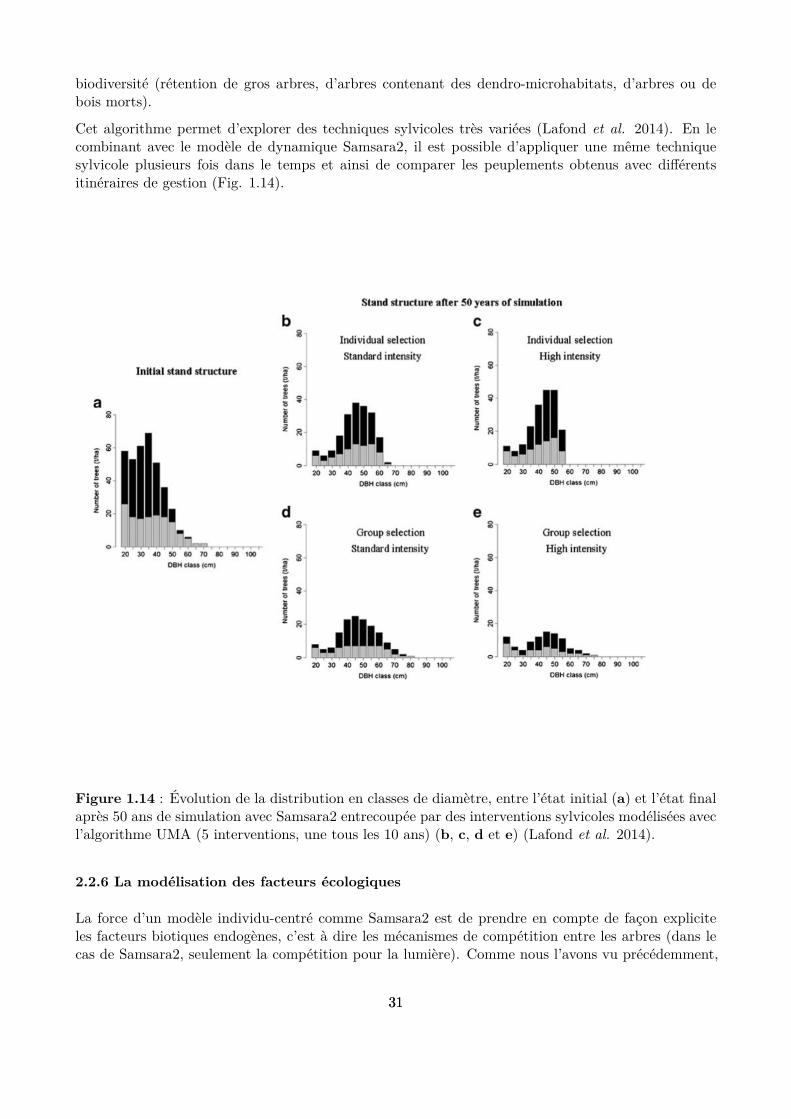
Cet algorithme permet d’explorer des techniques sylvicoles très variées (Lafond et al. 2014). En lecombinant avec le modèle de dynamique Samsara2, il est possible d’appliquer une même techniquesylvicole plusieurs fois dans le temps et ainsi de comparer les peuplements obtenus avec diférentsitinéraires de gestion (Fig. 1.14).
Figure 1.14 : Évolution de la distribution en classes de diamètre, entre l’état initial (a) et l’état inalaprès 50 ans de simulation avec Samsara2 entrecoupée par des interventions sylvicoles modélisées avecl’algorithme UMA (5 interventions, une tous les 10 ans) (b, c, d et e) (Lafond et al. 2014).
2.2.6 La modélisation des facteurs écologiques
La force d’un modèle individu-centré comme Samsara2 est de prendre en compte de façon expliciteles facteurs biotiques endogènes, c’est à dire les mécanismes de compétition entre les arbres (dans lecas de Samsara2, seulement la compétition pour la lumière). Comme nous l’avons vu précédemment,
3131
la gestion irrégulière est également simulée de façon ine avec Samsara2, à l’aide d’algorithmes desylviculture. Parmi les facteurs abiotiques, seule la lumière est prise en compte de façon explicitedans Samsara2 et aucun facteur biotique exogène n’est modélisé dans ce modèle. L’intégration ou nonde ces diférents facteurs dans le processus de modélisation sont des choix pragmatiques faits lors dudéveloppement du modèle (Courbaud et al. 2015) et qui sont liés à la hiérarchisation des facteursselon leur importance dans le fonctionnement de ces communautés. Ces choix ont été faits en amontde cette thèse et constituaient un héritage à prendre en compte.
Cependant, les questionnements scientiiques liés aux changements climatiques requièrent de modéliserde façon explicite comment la démographie varie en fonction du climat, ain de pouvoir réaliser desprojections de l’évolution des forêts en réponse à ces changements (Fontes et al. 2010). A cet égard,l’utilisation d’autres modèles de dynamique forestière intégrant déjà ces processus (Bugmann 2001)pourrait apparaître comme préférable au premier abord. Cependant, le modèle Samsara2 et sesmodules de gestion ofrent des fonctionnalités qui lui sont propres pour étudier diférentes stratégies degestion irrégulière de façon ine à l’échelle du peuplement (Lafond et al. 2014), ce qui nous intéresse plusparticulièrement dans cette thèse. Tout autre modèle aurait donc nécessité également des améliorationstechniques pour aborder cette problématique particulière. Il nous a donc paru plus eicace d’utiliserle modèle Samsara2 que nous connaissons bien et de le développer pour qu’il puisse répondre auxquestionnements liés aux changements climatiques.
L’enjeu est donc de pouvoir faire varier les paramètres démographiques sensibles dans Samsara2 enfonction de variables climatiques. Ce travail de calibration est délicat car, comme nous l’avons vu, lesdiférents facteurs écologiques interagissent sur la dynamique forestière et il est donc diicile d’isolerl’efet du climat sur les variations de cette dynamique. A cet égard, la calibration par ABC à partir desdonnées de gestion forestière se révèle intéressante car elle ofre la possibilité d’explorer la dynamiquepassée de peuplements forestiers situées dans des conditions climatiques contrastées tout en tenantcompte des facteurs clés ayant inluencé cette dynamique (densité des peuplements, composition enespèce, intensité de coupes).
2.3 Structuration de la thèse
2.3.1 Objectifs
Les objectifs de la thèse sont donc de :
• développer, formaliser et optimiser une méthode de calibration de Samsara2 à l’aide de donnéeshistoriques et de l’ABC ;
• documenter la variabilité démographique en forêt de montagne et quantiier les relations entreprocessus démographiques des trois espèces étudiées et facteurs climatiques ;
• projeter les efets de diférentes stratégies de sylviculture sur les biens et services fournis par cesforêts dans un contexte de changement climatique.
Ces trois objectifs sont abordés successivement et dans cet ordre dans les parties 2, 3 et 4 de cemanuscrit.
2.3.2 Hypothèses de travail
Voici les hypothèses de travail répondant aux trois grands objectifs de la thèse :
3232

H1 : la méthode ABC devrait permettre de calibrer les paramètres les plus inluents d’un modèlecomplexe comme Samsara2.
Il existe de nombreuses pistes pour réduire le nombre de simulations à réaliser pour estimer desparamètres par ABC. Cette méthode devrait donc être utilisable avec Samsara2.
H2 : le climat, et en particulier la température, devrait avoir un rôle déterminant sur la dynamiquede ces peuplements forestiers.
La température devrait être le facteur climatique le plus inluent sur la croissance des peuplements.La régénération des peuplements devrait également dépendre fortement des conditions climatiques.
H3 : la réduction de la densité des peuplements devrait permettre d’adapter les peuplements à unclimat plus chaud et plus sec mais pourrait dégrader certains services écosystémiques.
Une densité d’arbres moins élevée devrait être favorable dans des climats secs car la consommationd’eau par le peuplement serait alors moins importante. Par contre, certains services écosystémiquescomme la protection contre la chute des blocs ou la conservation de la biodiversité pourraient êtredégradés par la réduction de la densité du fait du rajeunissement des peuplements.
3333
3 - Partie 1 : Origines et nature des données utilisées
3.1 Préambule
L’objectif de cette partie est de mieux cerner les limites de ce travail liées aux données utiliséesmais également de permettre à ceux qui voudront les réutiliser pour d’autres travaux de savoir où etcomment ces données ont été collectées. Elle ne contient donc aucun élément d’analyse scientiique,mais le temps et l’énergie consacrés à la récupération de ces données méritaient une partie dédiéedans ce manuscrit. Cette présentation pourrait permettre un gain de temps lors de futurs projets derecherche.
3.2 Origines et nature des données utilisées
3.2.1 Données historiques de gestion
3.2.1.1 Généralités
En France, toutes les forêts publiques et les forêts privées de grande taille font l’objet d’un pland’aménagement, qui organise les opérations sylvicoles à efectuer au sein de la forêt. A intervallesde temps réguliers, les gestionnaires forestiers rédigent une révision de ce plan d’aménagement, quidonne les instructions sur les traitements sylvicoles à efectuer sur la forêt pour la période s’étalantde la date de cette révision à la suivante. La forêt est subdivisée en parcelles, qui représentent desunités de gestion : les informations sur l’état de la forêt et les coupes prévues sont déinies à cetteéchelle. A l’occasion de la révision du plan d’aménagement, les gestionnaires efectuent un recensementdes arbres présents dans le peuplement (appelé inventaire), selon des méthodes qui varient selon lesforêts et dans le temps. Ce sont les données chifrées issues de ce recensement qui nous intéressent ici,puisqu’elles donnent des informations quantitatives sur les arbres présents dans chacune des parcellesde la forêt, à intervalles de temps réguliers et parfois sur de longues périodes. Les autres informationsmentionnées dans le plan d’aménagement et ses révisions (description qualitative des peuplements etdu sol, évolution du parcellaire, …) sont également souvent utiles comme informations contextuelles.
Dans le cas de l’ONF, les gestionnaires sont également tenus de noter toutes les opérations qui ontété faites sur les peuplements dans l’intervalle de temps entre deux révisions du plan d’aménagement.Ces documents sont couramment désignés par le terme “sommiers”. Les gestionnaires privés fontégalement ce type de suivi, indispensable lui aussi pour maintenir une gestion correcte. Les coupes etautres récoltes d’arbres réalisées sont notamment comptabilisées dans ces documents. Les coupes sontgénéralement renseignées par un nombre et un volume d’arbres récoltés. Il s’agit ici de la deuxièmesource de données qui nous est utile comme complément aux inventaires forestiers. En efet, enayant des informations sur les efectifs à deux dates données ainsi que sur les arbres retirés dans lapériode entre les deux inventaires, il est possible d’en déduire des informations sur la démographiedu peuplement (croissance, régénération, mortalité) (Csillery et al. 2013 ; Courbaud et al. 2015).Dans ces documents, il y a également un grand nombre d’informations qui se révèlent utiles pourcomprendre et reconstituer au mieux la gestion passée des parcelles.
3.2.1.2 Archives de gestion de l’ONF
L’ONF est tenu de conserver les plans d’aménagement et toutes les révisions indéiniment et de con-server les sommiers sur toute la période de validité d’une révision. Pour beaucoup de forêts, il est donc
3434
relativement facile de retrouver les plans d’aménagement et leurs révisions depuis la date de soumis-sion de la forêt au régime forestier. Il est beaucoup plus diicile de retrouver les sommiers anciens quin’ont souvent pas été conservés une fois passée la révision du plan d’aménagement. C’est la disponi-bilité de ces sommiers qui limite donc le nombre de forêts et la durée de l’historique des données pourlesquelles des données exhaustives sont disponibles. Bien entendu, d’autres contraintes inhérentes àla recherche d’archives viennent compliquer la recherche de ces documents historiques : déplacementsdes archives, absence de classement rigoureux, destruction des documents par des causes diverses, …La combinaison de ces contraintes limite fortement les forêts pour lesquelles il existe des données dequalité sur de longues périodes de temps (i.e. sur la durée de plusieurs révisions d’aménagement).
3.2.1.2.1 Documents collectés par Anne-Lise Bartalucci
La recherche de ces archives de l’ONF a été initiée à l’IRSTEA de Grenoble et a fait l’objet d’unstage réalisé par Anne-Lise Bartalucci. Un nombre important de documents d’archives de l’ONF aété collecté à cette occasion et archivé dans des tableaux au format excel. Cette source de données aconstitué une base de départ très intéressante pour cette thèse.
3.2.1.2.2 Données supplémentaires (archives et terrain)
Dés le début de la thèse, nous avons consacré beaucoup de temps à augmenter cette base de don-nées initiale ain d’explorer une large gamme de conditions environnementales. Étant données lescontraintes mentionnées précédemment sur la recherche de ces documents historiques, nous avonsadopté une approche plutôt pragmatique : avec l’aide de collègues de l’ONF (Thierry Sardin, Ex-pert national sylvicultures, Thomas Villiers, Responsable aménagement pour le Sud Ouest, CatherineRiond et Jacques Fay, Pôle R&D de Chambéry, Christine Deleuze et Didier François, Pôle R&D deDôle), nous avons contacté un maximum d’agences ONF pour savoir lesquelles avaient conservé desarchives de façon adéquate et étaient prêtes à collaborer avec IRSTEA pour cette thèse. Les retoursont été peu nombreux, mais généralement fructueux, et nous ont permis d’enrichir le jeu de donnéesavec des forêts situées dans des conditions environnementales diférentes. Nous avons notammentrécupéré des archives pour les forêts communales d’Aussurucq et d’Ordiarp (Pyrénées-Atlantiques),gérées par Georges Rivet, pour la forêt domaniale de Massat (Ariège), gérée par Patrick Guillon, ainsique d’autres archives pour des forêts de Savoie, inutilisées pour cette thèse mais conservées dans la basede données. A l’issue de ces recherches, nous pensons qu’il serait possible de récupérer des archivespour un grand nombre d’autres forêts. J’encourage mes successeurs à continuer cette quête, certeslaborieuse mais riche en contacts et en émotions propres à toute recherche de trésors cachés !
En parallèle, au cours des étés 2014 et 2015, nous avons réalisé nous-mêmes des inventaires com-plémentaires avec l’aide de techniciens IRSTEA (Sophie Labonne, Eric Mermin et Pascal Tardif) etd’un stagiaire (Valentin Berlioux) dans les forêts d’Engins, de Queige et de Massat. Cette phase ter-rain a permis là aussi d’enrichir le jeu de données, en allongeant la période de temps de l’historiquedes peuplements et en procurant des inventaires plus précis que ceux réalisés par l’ONF. La réali-sation d’inventaires en plein par les personnels des instituts de recherche dans le futur apporte uneréelle valeur ajoutée aux documents d’archives, d’autant plus que l’ONF n’a souvent plus les moyensde réaliser elle-même ces inventaires. Cette activité terrain est peu technique et requiert seulementune bonne endurance, mais est très chronophage. Les données collectées fournissent par contre desperspectives intéressantes d’un point de vue recherche.
3.2.1.3 Autres sources de données historiques
3535

3.2.1.3.1 Groupement forestier privé dans le Jura
Les forêts gérées par ce groupement privé sont situées sur le premier plateau jurassien (environ 500 md’altitude) et sont gérées par la méthode du contrôle depuis plus de 40 ans (le premier plan de gestiondate de 1976). La méthode du contrôle consiste à inventorier en plein les parcelles, puis à procéder àune coupe immédiatement après en essayant de s’approcher au mieux d’une distribution en taille desarbres parfaitement irrégulière. Pour chaque année d’intervention sur une parcelle (environ tous les10 ans), un inventaire et un bilan de coupes ont été réalisés et les données correspondantes ont ététoutes consignées et conservées depuis 1976. Ce jeu de données constitue donc un complément trèsintéressant aux archives de l’ONF, car les forêts de ce groupement sont situées dans des conditions pluschaudes (dues à une altitude plus basse) que les forêts de l’ONF pour lesquelles nous avions obtenudes données.
3.2.1.3.2 Cabinet Leforestier Ltd.
Ce cabinet gère l’exploitation d’un certain nombre de forêts de montagne sous un régime de futaiejardinée. M. Leforestier a fourni des données de gestion permettant de reconstituer l’historique de 21peuplements dans 4 forêts situées dans les Alpes (massif de Belledonne), dans le Jura et dans le MassifCentral (Cantal). Ces données ont l’inconvénient d’être restreintes à une période relativement courte(l’inventaire le plus ancien remonte à 1986). Ces données ont été archivées avec les autres, mais, enraison de leur récupération tardive (récupération des données complètes seulement en Mars 2016) etde leur période de temps restreinte, elles ne font pas partie des analyses présentées dans la suite decette thèse.
3.2.1.3.3 Autres suivis de gestion (Slovénie)
Les données collectées par l’Université de Ljubljana en Slovénie dans le cadre du projet ARANGE(Klopcic, Jerina & Boncina 2010) ont également été utilisées dans cette thèse. Ces données sontsimilaires à celles de l’ONF, excepté les bilans de coupe qui sont informés par classes de diamètre etnon simplement par un nombre et un volume d’arbres récoltés.
3.2.1.3.4 Placettes de suivi permanentes (Suisse)
Dans le cadre d’un partenariat avec l’Institut fédéral de recherches sur la forêt, la neige et le paysage(WSL) de Birmensdorf (près de Zurich en Suisse), nous avons intégré au jeu de données 16 placettesforestières suivies sur le très long terme (les plus anciennes sont suivies depuis 1905) par le WSL. Ilne s’agit plus ici à proprement parler de données de gestion puisqu’il s’agit de placettes de recherche.Cependant, leur grande taille (un hectare en moyenne) et le fait qu’elles soient exploitées en gestionirrégulière font qu’elles sont homogènes avec les autres données historiques de gestion. Par contre,s’agissant de placettes de recherche, les données sont bien plus riches que les autres données de gestion: le statut et le diamètre des arbres sont suivis individuellement, avec des mesures tous les 5 ans. Cessuivis ofrent des perspectives de recherche très riches et tout leur potentiel est loin d’avoir été exploitédans le cadre de cette thèse.
3.2.2 Données environnementales
Les données historiques de gestion collectées étant situées dans diférents pays, nous avons utilisédiférentes sources pour quantiier les variables environnementales décrivant les milieux dans lesquels
3636

se trouvent les parcelles forestières. Il a donc fallu procéder à un important travail d’homogénéisationen vue de leur utilisation dans le cadre de cette thèse.
3.2.2.1 Données climatiques
3.2.2.1.1 Données du modèle SAFRAN
Selon les informations issues du site Internet du Centre National de Recherches Météorologiques, “lemodule d’analyse objective SAFRAN (Système d’Analyse Fournissant des Renseignements Adaptés àla Nivologie) (Durand et al. 1993) [a été] initialement développé au CNRM/CEN pour des besoinsd’estimation opérationnelle des risques d’avalanche en zone montagneuse” (SAFRAN 2016). Les don-nées de ce modèle sont utilisées maintenant dans bien d’autres disciplines, notamment en écologie.Grâce à une interpolation sur les stations de mesures existantes, le modèle fournit un ensemble devariables climatiques sur un maillage de 8 km x 8 km en France métropolitaine et en Suisse (soit 9892points). Les données sont journalières et disponibles du 01/08/1958 jusqu’à aujourd’hui.
Dans le cadre de cette thèse, seules les données journalières de température et de précipitation ont étéutilisées. Pour chaque peuplement étudié, les variables climatiques mensuelles ont été moyennées surla période commune entre la période historique délimitée par la date de l’inventaire le plus ancien etcelle de l’inventaire le plus récent et la période de disponibilité des données SAFRAN. Par exemple,pour un peuplement dont les dates des inventaires utilisés sont 1931 et 1980, la période commune est1958-1980.
3.2.2.1.2 Données du projet DRIAS
Le projet DRIAS (acronyme de “Donner accès aux scénarios climatiques Régionalisés français pourl’Impact et l’Adaptation de nos Sociétés et environnements”), qui a été mis en oeuvre de 2009 à 2012,a permis de mettre à disposition du public et des organismes de recherche les “scénarios climatiquesrégionalisés réalisés dans les laboratoires français de modélisation du climat” (DRIAS 2016a). Lapériode projetée court jusqu’en 2100 ; la maille géographique et le pas de temps sont les mêmes queceux de SAFRAN, mais elles ne concernent que la France métropolitaine. Trois des quatre scénarios(Representative Concentration Pathway, RCP) élaborés par le Groupe d’experts intergouvernementalsur l’évolution du climat (GIEC) dans son cinquième rapport (IPCC 2014a) ont été utilisés pourproduire ces données : RCP2.6, RCP4.5 et RCP8.5. Le chifre après RCP correspond au forçageradiatif en 2100 (exprimé en W.m-2) résultant du niveau d’émission de gaz à efet de serre choisi pourle scénario. Les données sont librement disponibles sur le site Internet de la DRIAS (DRIAS 2016b).Nous les avons utilisées dans la quatrième partie de la thèse, dédiée aux projections de la dynamiqueforestière dans le futur.
3.2.2.1.3 WorldClim
Les données WorldClim (Hijmans et al. 2005 ; WorldClim 2016) ont été utilisées pour les peuplementshors zone SAFRAN (i.e. pour les peuplements slovènes). Dans ces données librement accessibles surInternet, les valeurs de température et de précipitations sont moyennées sur la période 1960-1990 puisinterpolées sur une maille d’environ 1 km2 pour le monde entier à partir de mesures faites dans unlarge réseau de stations météorologiques.
3.2.2.2 Autres données environnementales
3737

3.2.2.2.1 Aménagements forestiers
Comme mentionné précédemment, les plans d’aménagement fournissent un certain nombred’informations sur l’environnement abiotique dans lequel les peuplements se situent. Ces informationssont cependant hétérogènes entre les diférentes forêts. La géologie grossière du lieu (géomorphologieet composition de la roche mère) et les conditions climatiques (a minima des informations qualita-tives sur le type de climat) sont par contre toujours indiqués, et souvent également des informationsqualitatives sur le sol (profondeur, hétérogénéité, teneur en roches, …).
3.2.2.2.2 ONF
Le site Internet de l’ONF donne accès aux données géographiques permettant de connaîtrel’emplacement de toutes les parcelles qu’elle gère (ONF 2016). Il s’agit de couches utilisables avecun système d’information géographique (SIG). Ces données nous ont permis d’obtenir toutes les in-formations géographiques et topographiques sur les parcelles gérées par l’ONF (longitude, latitude,altitude, pente, exposition).
3.2.2.2.3 SILVAE
L’AgroParisTech a mis en ligne en 2014 un ensemble de données environnementales geolocaliséesissues de leurs études sur les données de l’IFN. Le site Internet difusant ces données est le portailSILVAE (acronyme signiiant “Système d’Informations Localisées sur la Végétation, les Arbres etleur Environnement”). Ce portail donne accès à des couches SIG où un grand nombre de variablesclimatiques et pédologiques ont été interpolées à partir des mesures faites par l’IFN.
3838

4 - Partie 2 : Calibration du modèle Samsara2 par Calcul BayésienApproché
Article associé : Approximate Bayesian computation to recalibrate individual-based models with popu-lation data: Illustration with a forest simulation model (Lagarrigues et al. 2015) (Article publié dansEcological Modelling - Annexe A)
4.1 Problématiques et objectifs
Dans cette première partie, l’objectif était de développer et d’optimiser une méthode permettant decalibrer par ABC les paramètres démographiques les plus sensibles de Samsara2 à partir de donnéeshistoriques de gestion acquises dans un ensemble de parcelles forestières. Nous nous sommes doncfocalisés sur une seule parcelle dans cette partie (Parcelle 24 de la forêt de Prénovel).
L’ABC se base habituellement sur la réalisation d’un grand nombre de simulations du modèle (plusieurscentaines de milliers), ce qui s’est rapidement avéré problématique étant donnés les temps de calculimportants pour reproduire la dynamique historique avec Samsara2. Le premier objectif de cettepartie était donc d’optimiser la méthode de calibration par ABC pour qu’elle soit fonctionnelle avecun modèle gourmand en temps de calcul. D’autre part, Samsara2 fonctionne avec un grand nombrede paramètres et il était évident que certains interagiraient sur les statistiques résumantes, qui ont étédéinies en fonction de l’information fournie par les données de gestion. Le second objectif était doncd’adapter la méthode de calibration par ABC de façon à ce qu’elle permette de calibrer un modèle avecun grand nombre de paramètres à partir de données peu informatives. Il s’agissait ici de débloquerces deux verrous méthodologiques liés à l’utilisation de l’ABC avec un modèle complexe.
4.2 Questions spéciiques abordées
1. Combien et quels paramètres pouvons-nous recalibrer précisément avec des données peu infor-matives ?
2. Combien de simulations sont requises pour obtenir une convergence raisonnable des distributionspostérieures estimées par l’ABC ?
3. Quelle est la variabilité des prédictions du modèle après la recalibration ?
4.3 Principaux résultats
La méthode de calibration testée ici repose sur une étape préliminaire aux simulations ABC, consistantà réaliser une analyse de sensibilité pour détecter les paramètres les plus inluents. L’étape suivantea consisté à mettre en oeuvre la calibration ABC sur une seule parcelle en faisant varier le nombrede paramètres de Samsara2 estimés. Nous avons combiné une méthode de sélection de modèle et desconsidérations plus qualitatives pour choisir le nombre optimal de paramètres à estimer.
Nos analyses ont démontré que deux paramètres (un paramètre de croissance et un paramètre derégénération) par espèce pouvaient être estimés à partir de données de gestion forestière. Nous avonsdémontré également que cette méthode permettait de restreindre grandement le nombre de simulationsà réaliser (20,000). Ces résultats, issus de la calibration sur les données historiques d’un seul peuple-ment forestier, ont permis d’envisager le déploiement de cette méthode de calibration sur l’ensembledes données comportant environ 200 parcelles.
3939
D’autre part, nous avons constaté que la variabilité des prédictions du modèle après recalibration étaitprincipalement causée par la stochasticité du modèle, et beaucoup moins par la recalibration par ABCet les incertitudes sur la calibration initiale. Cela nous a assuré de la qualité de la calibration dumodèle à partir de nos données peu informatives.
4.4 Éléments de discussion complémentaires
4.4.1 Analyse de sensibilité
Pour ce travail de calibration, nous avons utilisé une analyse de sensibilité réalisée précédemment(Courbaud et al. 2015). L’analyse de sensibilité est un préliminaire primordial à ce travail de re-calibration d’un modèle complexe comme Samsara2, notamment pour déinir l’ordre de priorité desparamètres à recalibrer et pour dimensionner la puissance de calcul nécessaire. Aussi, en complémentde l’analyse de sensibilité sur les paramètres démographiques, une autre analyse de sensibilité a égale-ment été faite sur les paramètres techniques du modèle (taille des cellules de sol, aire du peuplement,pas de temps pour le calcul de la distribution de la lumière, …) conditionnant la discrétisation del’espace et du temps et ayant donc une inluence importante sur le temps de calcul et potentiellementégalement sur les sorties du modèle. Ce travail a permis d’optimiser la méthode de calibration, ensélectionnant pour ces paramètres de discrétisation les modalités qui permettaient de réduire le pluspossible les temps de calcul sans modiier signiicativement les résultats des simulations. Ce travailn’étant pas au coeur de la thèse, il n’a été appliqué que sur une seule parcelle (la même que celle qui aété utilisée dans cette partie), et il est possible que les résultats aient été diférents avec d’autres par-celles ayant des périodes de temps diférentes et/ou des structures en taille des arbres diférentes. A cetégard, pour de prochaines études, il paraît important de réaliser une analyse de sensibilité prenant encompte tous les paramètres du modèle et diférents états initiaux ain de mieux appréhender l’inluencedes diférents paramètres et optimiser la méthode de calibration.
4.4.2 Retour sur le critère de sélection de modèles pour le nombre de paramètres
Nous avons utilisé le facteur bayésien (Kass & Raftery 1995) ain de sélectionner le nombre deparamètres à recalibrer, en suivant la méthode par régression logistique multinomiale proposée parBeaumont et al. (2008). Nous avions ainsi plusieurs modèles, avec 0, 2, 4 ou 6 paramètres calibrés.Cependant, l’utilisation du facteur bayésien pose problème dans cette situation car il est très sensibleà la largeur des distributions antérieures utilisées. Concrètement, des distributions plus larges auronttendance à favoriser les modèles avec peu de paramètres, alors qu’idéalement, la sélection du meilleurmodèle devrait être indépendante des distributions utilisées. Nous avons étudié plusieurs alternatives,notamment l’utilisation du DIC (Deviance Information Criterion) adapté pour l’ABC par Françoiset al. (2011). Cependant, les résultats obtenus étaient incohérents, et nous n’avons pas pu identiierla cause du problème car nous étions limités en nombre de simulations (la méthode d’estimation duDIC requiert de réaliser des simulations supplémentaires). Au inal, nous avons conservé le facteurbayésien, en combinant à cette approche quantitative des éléments d’analyse plus qualitative, notam-ment en analysant la qualité des prédictions des diférents modèles (comparaison des distributions ennombre d’arbres par classes de diamètre simulées et observées). Dans l’état actuel de ces travaux,nous n’avons pas trouvé de méthode statistique rigoureuse permettant de réaliser cette sélection dunombre de paramètres à calibrer indépendamment des distributions antérieures et du modèle utilisé.
4040
5 - Partie 3 : Variations démographiques de la dynamique forestière lelong de gradients environnementaux
Article associé : Demographic variability in spruce-ir-beech forest stands in Europe (Article en prépa-ration pour European Journal of Forest Research, Annexe B)
5.1 Problématiques et objectifs
Une fois obtenu un cadre de calibration du modèle Samsara2 suisamment robuste, reproductibleet cadré sur une parcelle test, cette méthode a été déployée sur un ensemble de parcelles d’étude.Ces parcelles sont caractérisées par des données de gestion forestière qui s’étalent sur une périodesuisamment longue (> 30 ans) et où le cumul des sapins, des épicéas et des hêtres représentent plusde 80% des arbres du peuplement en surface terrière. L’objectif ici était d’analyser si des variablesenvironnementales ont une inluence sur les processus démographiques simulés et avec quelle intensité.La bibliographie montre que la dynamique forestière est sensible aux variables environnementalescomme la température ou la disponibilité en eau mais met également en évidence des incohérencessur la réponse de la dynamique de l’épicéa, du sapin et du hêtre à ces facteurs. Le problème reposesur la prise en compte des facteurs multiples (comme la densité des arbres, le taux de mélange desespèces ou encore l’intensité de la gestion) qui inluencent cette dynamique des espèces et qui peuventdonc brouiller les réponses au climat. Le modèle Samsara2 permet de tenir compte explicitement defacteurs biotiques endogènes comme la structure en taille ou la surface terrière du peuplement. Notreapproche par calibration inverse d’un modèle individu-centré permet ainsi d’isoler les efets des autresfacteurs écologiques (dont le climat) sur les variations des processus démographiques à l’échelle desarbres en utilisant des données à l’échelle des peuplements.
5.2 Questions spéciiques abordées
1. Est-ce que la variabilité des paramètres de Samsara2 calibrés sur l’ensemble des parcelles estindépendante des facteurs biotiques endogènes, et notamment de la surface terrière ?
2. Est-ce que la variabilité entre forêt est plus grande que la variabilité intra-forêt, i.e est-ce queles variables macro-environnementales (déinies à l’échelle des forêts) permettent d’expliquer lamajeure partie de la variabilité de la dynamique forestière ?
3. Est-ce que les variables macro-environnementales habituellement utilisées ont des efets cohérentset signiicatifs sur la dynamique des trois espèces étudiées dans les conditions environnementalesconsidérées ?
5.3 Principaux résultats
Nos résultats ont montré que les variations du paramètre de croissance de Samsara2 entre les diférentesforêts sont indépendantes de la surface terrière du peuplement, qui est un bon indicateur indirect defacteurs biotiques endogènes comme la compétition des arbres pour la lumière. En ce qui concerne larégénération, la la surface terrière du peuplement n’avait pas d’inluence sur le taux de recrutementcalculé directement à partir des données et nos analyses n’ont pas permis de statuer sur l’eicacitéde la méthode sur cet aspect pour ce processus. Par ailleurs, il s’est avéré que la variabilité entreforêts est signiicativement plus grande que la variabilité entre parcelles d’une forêt (i.e. intra-forêt)seulement pour la croissance du sapin. Concernant les relations entre processus démographiques etfacteurs macro-environnementaux, la somme des degrés-jours de croissance (un indicateur basé sur
4141
la température) est le principal facteur inluençant la croissance du sapin. Cet indicateur permetégalement d’expliquer une part signiicative de la variabilité de la croissance de l’épicéa et de larégénération du sapin et de l’épicéa, mais plus faiblement que pour la croissance du sapin et avec desformes de réponse hétérogènes.
5.4 Éléments de discussion complémentaires
5.4.1 Hétérogénéité des données entre les diférentes forêts
L’hétérogénéité des données utilisées, en matière de qualité des données (contenus informatifs) et depériode temporelle (durée et dates des inventaires), s’est révélée être une diiculté importante danscette partie et il est possible qu’elle ait inluencé les résultats obtenus (notamment la faible réponse dela démographie aux variables climatiques). En efet, notre reconstruction de l’historique des parcellescomporte des simpliications et des hypothèses fortes, notamment sur la phase de régénération initiale(simulée sous hypothèse d’équilibre entre stade adulte et stades jeunes) et sur l’occurrence d’événementsextrêmes (considérées comme des coupes ordinaires). Or, l’état inal dépend d’autant plus fortement del’état initial que la période de simulation est courte et l’hétérogénéité des durées a donc pu introduireun biais. De même, les périodes temporelles de nos données ne recouvrent pas la date de certainsévénements extrêmes (comme la tempête de 1999 en France), ce qui pourrait également avoir biaisé lesrésultats de façon systématique entre diférentes forêts. Bien que nous ayons vériié que les résultatsétaient peu sensibles à la date des inventaires et à la période de temps entre les inventaires paranalyse de corrélations, une analyse plus détaillée serait nécessaire pour s’assurer que l’hétérogénéitédes données n’a pas une inluence signiicative sur les résultats. Il serait par exemple intéressantd’utiliser les données de suivi des parcelles du WSL (données les plus longues et les plus détaillées)pour analyser plus en détail cette problématique, par exemple en calibrant le modèle sur diférentespériodes temporelles ou encore en agrégeant plus ou moins les données pour étudier l’efet de diférentscontenus informatifs.
5.4.2 Modélisation paramétrique de la relation démographie / climat
D’un point de vue méthodologique, nous avions deux possibilités pour modéliser la relation démo-graphie / climat : déinir a priori les équations reliant paramètres démographiques de Samsara2 etles variables environnementales (méthode a priori), ou bien calibrer indépendamment chaque parcellepour obtenir un jeu de valeur de paramètres qui servirait ensuite de variable dépendante à relier auxvariables environnementales (méthode a posteriori). La méthode a posteriori a inalement été retenue,pour deux raisons. Premièrement, les temps de calcul ne permettaient pas d’explorer plusieurs types demodèles démographie / climat avec la solution 1. Or, nous voulions garder la possibilité d’explorer dif-férentes équations (équations linéaires, quadratiques, saturantes, …) pour ces modèles. Deuxièmement,il y avait un intérêt opérationnel à avoir un jeu de paramètres par parcelle, ain d’élargir la gamme despeuplements initiaux disponibles pour des simulations avec Samsara2 associés à des paramètres démo-graphiques qui reproduisent idèlement leur dynamique passée. Ce choix présente néanmoins plusieursinconvénients : cette méthode d’inférence des paramètres climatiques en deux étapes est plus complexeà appréhender et donc à expliquer ; elle ne permet pas d’intégrer de façon rigoureuse les diférentessources d’incertitude, comme la stochasticité de Samsara2 ou l’initialisation des peuplements, dansl’incertitude sur les paramètres des équations reliant démographie et climat. Il serait donc intéres-sant de vériier les résultats obtenus avec la méthode a posteriori avec ceux que nous obtiendrions enutilisant la méthode a priori, en utilisant les mêmes équations entre paramètres démographiques etclimat.
4242

6 - Partie 4 : Adaptation de la gestion forestière au changement clima-tique
Article associé : Stand-level management options to preserve goods and services provided by uneven-aged mountain forests in a context of climate change (Article en préparation pour Annals of ForestScience, Annexe C)
6.1 Problématiques et objectifs
La dernière partie de cette thèse aborde des aspects plus opérationnels en explorant diférentes straté-gies de gestion irrégulière dans un contexte de changement climatique. La problématique de cettepartie repose sur la complexité de déinir des stratégies d’adaptation de la gestion forestière en change-ment climatique, compte tenu des nombreux facteurs interagissant dans ce domaine. En efet, cettedémarche d’adaptation nécessite de tenir compte des diférents scénarios de changement climatiqueélaborés par le GIEC, des diférences entre peuplements en matière de démographie des espèces,de structure en taille et de composition spéciique et des diférents biens et services rendus par lesforêts. La complexité et la diversité de ces facteurs rend très diicile la déinition de recommandationsopérationnelles à l’échelle du peuplement pour les gestionnaires forestiers et les études existantes nefournissent donc souvent que des directives générales par grands types de peuplement. Par ailleurs, cer-taines études ont proposé de réduire fortement la densité des peuplements (déstockage) pour diminuerla consommation en eau des arbres et donc limiter les dégâts potentiels de sécheresses qui pourraientdevenir plus intenses et/ou plus fréquentes dans un proche avenir. Cependant, cette stratégie posequestion sur la fourniture de certains biens et services, notamment sur la conservation d’espèces ani-males et végétales inféodées aux peuplements matures ou sur la protection contre les risques naturels(chute de blocs rocheux, avalanches, érosion du sol).
L’objectif de cette partie est d’aborder spéciiquement la question de l’adaptation de la gestion ir-régulière des hêtraies-sapinières-pessières au changement climatique, en explorant de façon ine dif-férentes stratégies de gestion (dont une stratégie de fort déstockage) et en tenant compte des diférencesdémographiques à l’échelle du peuplement.
6.2 Questions spéciiques abordées
1. Pour quels peuplements la fourniture de biens et services est menacée par le changement clima-tique avec la gestion actuellement appliquée ?
2. Quel est l’efet d’un déstockage important des peuplements sur les biens et services fournis parles hêtraies-sapinières-pessières ?
3. Quels sont les leviers d’adaptation de la gestion à l’échelle du peuplement pour maintenir à unbon niveau les biens et services étant donnés les diférents scénarios de changement climatiqueet les disparités entre forêts et entre peuplements au sein des forêts ?
6.3 Principaux résultats
Pour ce qui concerne les hêtraies-sapinières-pessières actuellement situées dans des conditions mésiques,il apparaît dans nos projections que les indicateurs de biens et services varient fortement entre les peu-plements et entre les diférentes stratégies de gestion mais peu entre les diférents scénarios de change-ment climatique. Par contre, certains peuplements situés dans les zones les plus chaudes actuellement
4343

ainsi que les pessières pures sont identiiés comme vulnérables au changement climatique avec la ges-tion actuellement pratiquée, en particulier en cas de forte augmentation de la mortalité de l’épicéacausée par des attaques de bostryche.
Appliquer un déstockage important détériore fortement certains services et ne paraît donc pas appro-prié dans ces peuplements où la conservation de ces multiples services est importante. Une stratégiede gestion basée sur la priorisation de l’épicéa dans les récoltes permet de devancer les épisodes demortalité de cette espèce et donc d’améliorer généralement les indicateurs de biens et services par rap-port à la gestion actuellement préconisée, mais ne permet généralement pas d’atteindre une bonnequalité de ces biens et services.
La stratégie actuellement préconisée apparaît donc comme une bonne stratégie en comparaison desautres stratégies explorées dans cette étude, bien qu’elle ne permette pas de garantir le maintien detous les biens et services dans certains cas.
6.4 Éléments de discussion complémentaires
6.4.1 Problématique posée par les hêtraies-sapinières-pessières en marge chaude de leur airede distribution
La question de l’adaptation au changement climatique des hêtraies-sapinières-pessières en margechaude de leur aire de distribution n’a pas pu être convenablement abordée dans cette thèse. Enefet, il est très diicile de trouver des données historiques de gestion dans les situations chaudes car,d’une part, ces peuplements sont le plus souvent soumis à une gestion régulière et il est donc plus dif-icile d’obtenir un suivi exhaustif des opérations sylvicoles passées et d’autre part, d’autres espèces,comme le chêne, deviennent prépondérantes et le modèle Samsara2 n’est pas calibré pour ces espècesplus thermophiles. Pour explorer la dynamique future des peuplements dans cette situation et leurchangement de composition qui interviendra inévitablement, il s’avère nécessaire d’utiliser des mod-èles de dynamique forestière intégrant des espèces de plaine et/ou méditerranéennes et des processusde succession et d’immigration des espèces (Elkin et al. 2013; Snell et al. 2014 ).
6.4.2 Aller plus loin dans la prise en compte des spéciicités des peuplements
Les résultats des parties 3 et 4 de cette thèse mettent en évidence l’importance de la variabilitédes conditions environnementales entre les peuplements dans ces forêts de montagne. Le modèleSamsara2 permet d’en prendre un certain nombre en compte (les facteurs biotiques endogènes et latopographie) et le travail de calibration réalisé dans la partie 3 a permis de quantiier les variationsintra-forêt de croissance et de régénération. La prise en compte de ces facteurs permet de mettreen évidence dans la partie 4 que cette variabilité entre forêts et entre peuplements est déterminantesur la valeur des indicateurs de biens et services. Cependant, les projections faites dans la partie4 ignorent certaines spéciicités à l’échelle du peuplement qui sont pourtant importantes aux yeuxdes gestionnaires forestiers. Par exemple, l’historique de gestion, la fertilité du site, la distributionspatiale des espèces, la composition en espèce, l’accessibilité ou la présence d’aléas naturels inluencentles choix des gestionnaires en matière de surface terrière objectif à atteindre et de période de rotation.La prise en compte de ces éléments dans le modèle constitue une couche de complexité supplémentairemais il n’existe pas de diiculté insurmontable pour la mettre en oeuvre. En efet, ces informationssont souvent facilement disponibles auprès des gestionnaires ou dans les documents de gestion etil serait relativement aisé d’ainer les stratégies de gestion dans notre modèle grâce à la lexibilitéde l’algorithme UMA. Il s’agit là d’une perspective intéressante pour ainer les projections faites à
4444

l’échelle du peuplement et de mieux faire correspondre les recommandations faites avec les attentesdes gestionnaires forestiers.
4545
7 - Discussion générale
7.1 Retour et discussion sur les hypothèses
7.1.1 La méthode ABC permet de calibrer les paramètres les plus inluents d’un modèlecomplexe comme Samsara2
La calibration de modèles par ABC a connu un important succès au cours des 15 dernières années(pratiquement 1000 publications depuis 2002, cf. Fig. 4.1) et elle est aujourd’hui utilisée largementdans beaucoup de domaines scientiiques, avec une prédominance dans les sciences de l’écologie etde l’évolution biologique (Fig. 4.2) (Beaumont 2010). Ce succès s’explique notamment par les dii-cultés techniques de calibrer des modèles complexes où la vraisemblance ne peut pas être expriméeanalytiquement avec des techniques de modélisation classiques. L’autre avantage de l’ABC (et plusgénéralement des techniques de modélisation inverse) est de pouvoir calibrer tous les processus con-jointement et ainsi d’estimer les covariances entre processus. Cependant, cette méthode a été princi-palement utilisée avec des modèles demandant des temps de calcul faibles, car cette méthode baséesur un grand nombre de simulations peut décourager des modélisateurs non aguerris aux méthodesde calcul intensif (utilisation de fermes de calcul, techniques de parallélisation, …).
Dans cette thèse, nous avons développé une méthodologie qui permet de rendre cette méthode per-tinente pour de tels modèles en réduisant le nombre de simulations à réaliser. La principale carac-téristique de cette méthodologie est qu’elle requiert des étapes préliminaires. D’abord, les diférentsparamètres du modèle doivent être estimés à partir de données ou de bibliographie renseignant directe-ment sur les processus. Ensuite, il faut réaliser une analyse de sensibilité des paramètres du modèleaux données de calibration. Si cette analyse de sensibilité peut se révéler fastidieuse pour des modèlescomplexes, elle apporte des connaissances diverses sur le modèle qui peuvent être valorisées au-delàdu contexte de calibration par ABC (Courbaud et al. 2015). Enin, il est utile de réaliser un petitnombre de simulations du type de celles à réaliser pour l’ABC pour choisir les statistiques résumanteset pour préciser les distributions antérieures des paramètres à calibrer. Ces simulations permettentd’améliorer la précision des estimations par ABC qui seront faites par la suite et donc de limiter lenombre de simulations à réaliser (Blum et al. 2013).
4646
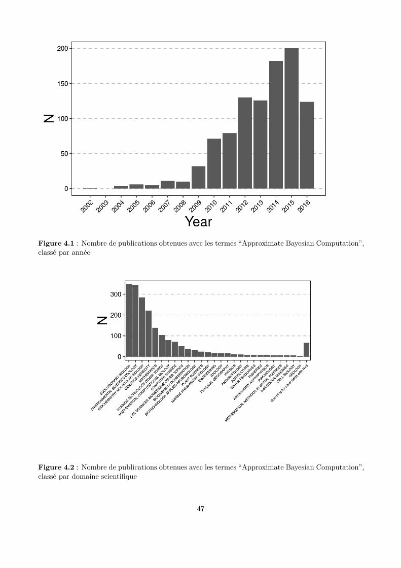
Figure 4.1 : Nombre de publications obtenues avec les termes “Approximate Bayesian Computation”,classé par année
Figure 4.2 : Nombre de publications obtenues avec les termes “Approximate Bayesian Computation”,classé par domaine scientiique
4747
Dans cette thèse, nous n’avons pas testé les algorithmes ABC séquentiels (Beaumont 2010; Marin et al.2012 ). En efet, bien que l’eicacité de ces algorithmes ne fasse aucun doute en matière de réduction dunombre de simulations à réaliser pour obtenir des estimations précises des distributions postérieures desparamètres, leur utilisation soulève de nouvelles diicultés en comparaison de l’algorithme standardde rejet. D’abord, le seuil d’acceptation des simulations doit être ajusté au fur et à mesure desitérations, ce qui implique une rélexion plus poussée sur ces seuils et probablement des tests dediférentes séquences de seuil. Ce travail préliminaire peut donc complexiier la mise en oeuvre del’ABC, bien que certains algorithmes ajustent automatiquement le seuil à chaque itération, à partirdu calcul d’un quantile sur la distribution des distances obtenues à l’étape précédente (Lenormand etal. 2013). Ensuite, l’aspect itératif de ces méthodes pose des problèmes techniques ardus en ce quiconcerne sa combinaison avec une ferme de calcul. En efet, il est relativement facile de paralléliserles simulations ABC avec l’algorithme de rejet : il suit d’échantillonner préalablement l’ensembledes valeurs de paramètres à simuler, puis de séparer cet ensemble dans des paquets (par exemple,10 simulations par paquet), de distribuer ces diférents paquets sur des noeuds de calcul diférents etinalement de regrouper tout une fois que tous les paquets sont traités. La diiculté avec les méthodesséquentielles est que l’ensemble de ce processus doit être réalisé plusieurs fois de façon automatique,et cette automatisation est soumise à de nombreuses contraintes techniques diiciles à résoudre surdes grandes fermes de calcul (Vaart et al. 2015), bien que des logiciels récents permettent de réduireces diicultés (Reuillon, Leclaire & Rey-Coyrehourcq 2013).
Avec l’ABC (et plus généralement avec toutes les méthodes de modélisation inverse), il est devenupossible de calibrer des modèles basés sur des processus à partir de données qui n’ont pas été spéci-iquement collectées dans ce but, et en particulier des données d’observation qui sont habituellementdes données de validation de modèle (Hartig et al. 2012). C’est ce que nous avons réalisé dans cettethèse, puisque certaines des données historiques de gestion que nous avons utilisées pour la calibrationont auparavant été utilisées pour évaluer le modèle Samsara2 (Courbaud et al. 2015). Dans le cadred’un stage de master, nous avons également réussi à calibrer d’autres paramètres de régénération deSamsara2 (Geofroy 2015) à partir de données de suivi de trouées collectées dans le cadre d’une autreétude (Fuhr 2015), ce qui constitue un autre exemple de calibration de modèle à partir de donnéesnon prévues pour cet usage. Ce genre de méthodes, en se popularisant et en devenant plus accessi-ble du fait du développement des outils de calcul, ofrent des perspectives très riche en matière decalibration de modèles.
7.1.2 La forme et l’intensité de la relation entre température et démographie dépend desespèces
Nous avons mis en évidence que la réponse des processus démographiques des arbres aux variablesclimatiques variait en forme et en intensité au sein des trois espèces étudiées. Cela remet en causela similarité de la réponse aux variables climatiques chez ces espèces écologiquement proches. Enefet, par manque de données de calibration, les relations entre démographie et climat sont souventsimilaires en forme et en intensité entre les diférentes espèces dans les modèles de dynamique forestière(Bugmann & Solomon 2000 ; Seidl et al. 2005). Nos résultats permettent donc de préciser les relationsentre démographie et climat pour ces trois espèces. Il est tout de même important de noter que nous neremettons pas en cause les limites thermiques et hydriques de distribution des espèces utilisées dansces modèles, qui permettent de simuler correctement les assemblages des communautés forestièresdans les forêts de montagne (Bugmann & Solomon 2000; Snell et al. 2014 ). Notre étude porte sur ladémographie des arbres entre les extrêmes (ni trop chaud, ni trop froid, ni trop sec, ni trop humide),donc dans les conditions que nous avons appelé “mésiques” où ces trois espèces peuvent se maintenirsans diiculté. Cependant, ces conditions mésiques s’étendent déjà sur de larges gradients climatiques,
4848
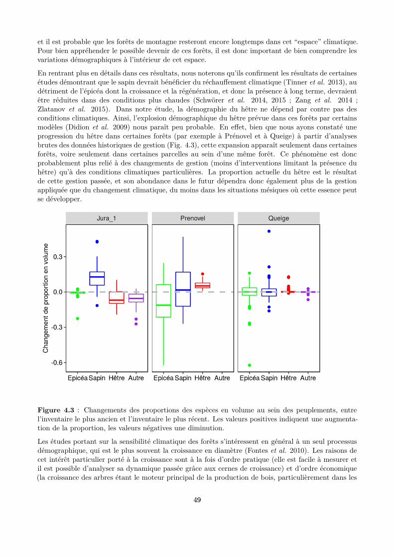
et il est probable que les forêts de montagne resteront encore longtemps dans cet “espace” climatique.Pour bien appréhender le possible devenir de ces forêts, il est donc important de bien comprendre lesvariations démographiques à l’intérieur de cet espace.
En rentrant plus en détails dans ces résultats, nous noterons qu’ils conirment les résultats de certainesétudes démontrant que le sapin devrait bénéicier du réchaufement climatique (Tinner et al. 2013), audétriment de l’épicéa dont la croissance et la régénération, et donc la présence à long terme, devraientêtre réduites dans des conditions plus chaudes (Schwörer et al. 2014, 2015 ; Zang et al. 2014 ;Zlatanov et al. 2015). Dans notre étude, la démographie du hêtre ne dépend par contre pas desconditions climatiques. Ainsi, l’explosion démographique du hêtre prévue dans ces forêts par certainsmodèles (Didion et al. 2009) nous paraît peu probable. En efet, bien que nous ayons constaté uneprogression du hêtre dans certaines forêts (par exemple à Prénovel et à Queige) à partir d’analysesbrutes des données historiques de gestion (Fig. 4.3), cette expansion apparaît seulement dans certainesforêts, voire seulement dans certaines parcelles au sein d’une même forêt. Ce phénomène est doncprobablement plus relié à des changements de gestion (moins d’interventions limitant la présence duhêtre) qu’à des conditions climatiques particulières. La proportion actuelle du hêtre est le résultatde cette gestion passée, et son abondance dans le futur dépendra donc également plus de la gestionappliquée que du changement climatique, du moins dans les situations mésiques où cette essence peutse développer.
Figure 4.3 : Changements des proportions des espèces en volume au sein des peuplements, entrel’inventaire le plus ancien et l’inventaire le plus récent. Les valeurs positives indiquent une augmenta-tion de la proportion, les valeurs négatives une diminution.
Les études portant sur la sensibilité climatique des forêts s’intéressent en général à un seul processusdémographique, qui est le plus souvent la croissance en diamètre (Fontes et al. 2010). Les raisons decet intérêt particulier porté à la croissance sont à la fois d’ordre pratique (elle est facile à mesurer etil est possible d’analyser sa dynamique passée grâce aux cernes de croissance) et d’ordre économique(la croissance des arbres étant le moteur principal de la production de bois, particulièrement dans les
4949
forêts en gestion régulière). Cependant, d’un point de vue écologique, cet intérêt quasi exclusif portéà la croissance pose problème dans certaines situations, notamment lorsqu’il s’agit d’évaluer et d’agirsur les diférents services rendus par les forêts (Lindner et al. 2010). Dans notre cas, nous avions pourobjectif d’étudier la dynamique des peuplements irréguliers de montagne sur du long terme (environ100 ans), ce qui nécessite de tenir compte conjointement de plusieurs processus démographiques, etdonc notamment de la régénération. La calibration conjointe de plusieurs processus démographiquesdans les modèles de dynamique forestière est encore balbutiante (Hartig et al. 2014) et cette thèseapporte des éléments concrets pour la mettre en oeuvre.
7.1.3 Une forte réduction des densités n’est pas pertinente dans les forêts de moyennemontagne
Dans les forêts étudiées dans le cadre de cette thèse, l’abaissement des densités à des niveaux faibles(15 m2.ha-1) n’apporte pas les bénéices envisagés dans d’autres contextes (Legay et al. 2007 ; Elkinet al. 2015). La raison principale est que la disponibilité en eau n’est actuellement pas limitantedans ces forêts, ce qui restreint la portée de nos résultats à cette situation. Dans les forêts de bassealtitude, la question de la disponibilité en eau dans le futur est pourtant sensible (Hlásny et al. 2011;Elkin et al. 2013 ; Zang et al. 2014 ; Keenan 2015 ). Néanmoins, il est probable que, dans leshêtraies-sapinières-pessières de basse altitude, le problème de la disponibilité en eau ne soit pas liéà la densité des peuplements mais bien plutôt à la sensibilité intrinsèque de ces espèces au manqued’eau (Piedallu et al. 2009). Dès lors, la baisse de la densité ofrirait la possibilité à d’autres espècesmoins sensibles de s’installer, et cette mesure associée à d’autres (conservation des espèces compagnes,plantations) permettrait de remplacer graduellement la composition en espèce dans ces peuplementset de conserver les services écosystémiques forestiers dans des conditions plus sèches. Cependant,il demeure qu’une baisse durable de la densité aura des conséquences néfastes sur d’autres servicestels que la protection contre les chutes de bloc ou la conservation d’espèces typiquement forestièrestelles que les champignons et les insectes saproxyliques (qui se nourrissent de bois en décomposition)généralement inféodées à des forêts matures et denses, et cette mesure devrait donc être considéréeavec précaution.
Il est important de noter que les projections faites dans cette étude ne sont iables que dans les scénariosoù les forêts étudiées restent dans des conditions mésiques, qui sont déinies dans cette thèse commela zone climatique que nous avons pu explorer avec nos données. Dans le cas des scénarios RCP2.6et RCP4.5 du GIEC, nos parcelles restent généralement dans ces conditions mésiques. Par contre,dans le scénario RCP8.5, il apparaît que pratiquement toutes les parcelles étudiées sortent de cesconditions. Dans le cas de ce scénario, nos projections sont donc dans une situation d’extrapolation,qui est problématique car les processus reliant démographie et climat dans le modèle que nous avonsutilisé sont très simplistes. De nombreux modèles intégrant une représentation explicite des processusreliant climat et physiologie des arbres ont été développés pour explorer de façon plus robuste ce genrede situation (Dufrêne et al. 2005 ; Deckmyn et al. 2008; Fontes et al. 2010 ). Cependant, ces modèlesécophysiologiques sont encore peu utilisés pour explorer la dynamique à long terme des peuplementset ne permettent pas à notre connaissance de simuler des stratégies de gestion ines et variées commecelles que nous avons explorées dans cette étude.
Cette thèse met en évidence que la gestion préconisée dans les guides de sylviculture pour les hêtraies-sapinières-pessières jardinées (Gauquelin & Courbaud 2006) constitue une bonne sylviculture pours’adapter au changement climatique dans la plupart des cas. Cependant, ce type de sylviculture n’estpas toujours appliqué en pratique pour diverses raisons, la plus importante étant la topographie deces forêts de montagne qui limite l’accessibilité à certaines parcelles et donc leur gestion. Pour adapterla gestion de ces forêts au changement climatique, il serait donc plus pertinent de chercher comment
5050

mettre en oeuvre eicacement une gestion qui est déjà bien maîtrisée et adaptée à ce contexte plutôtque de chercher des options de gestion radicalement nouvelles. Plus largement, la gestion irrégulièreou jardinée constitue aujourd’hui une alternative intéressante à la gestion régulière car elle permet deconserver les services écosystémiques forestiers, d’assurer la résilience des peuplements et elle laisse delarges possibilités d’adaptation en cas de dépérissement d’une espèce (Schütz 1997 ; Cordonnier et al.2008 ; Diaci, Kerr & O’Hara 2011 ; Pretzsch et al. 2012; Bouriaud et al. 2014 ). Le maintien de ce typede gestion et la transformation des peuplements mono-spéciiques réguliers en peuplements irréguliersmélangés, encore peu envisagés dans les études portant sur l’adaptation de la gestion forestière auchangement climatique (Lindner et al. 2014 ; Keenan 2015), mériteraient davantage d’attention ainde pouvoir être appliqués plus largement.
7.2 Synthèse des forces et des limites des données et méthodes utilisées
Nous proposons ici une synthèse des limites et des perspectives qui ont été identiiées tout au long dece manuscrit. Les diférents sujets regroupés ici concernent les données, les méthodes et le type demodèle que nous avons utilisés. Nous présentons les forces et les limites de chaque objet, par rapportà d’autres alternatives (comme les données expérimentales en comparaison des données historiques degestion).
5151
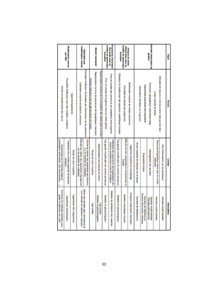
5252
Table 1 : Forces et limites des types de données et des méthodes utilisés.
7.3 Perspectives
7.3.1 Utiliser toutes les informations disponibles dans les données historiques de gestion
L’efort fourni pour développer la méthode au cours de cette thèse n’a pas permis d’utiliser toutesles informations disponibles dans ces données de gestion. Voici les informations qu’il serait possibled’utiliser pour prolonger le travail de calibration de Samsara2 à partir de ces données :
• Utiliser les inventaires intermédiaires : dans cette thèse, nous avons considéré uniquementl’inventaire le plus ancien et le plus récent pour chaque parcelle ain d’explorer la période tem-porelle la plus large possible, avec l’objectif de pouvoir ainsi calibrer les paramètres de régénéra-tion. En utilisant les distributions postérieures obtenues dans le cadre de cette thèse commeinformation a priori, il serait intéressant d’utiliser aussi les inventaires intermédiaires (lorsqu’ilsexistent) pour réduire les incertitudes sur les paramètres de croissance.
• Utiliser les informations sur les produits récoltés : pour les parcelles gérées par l’ONF et lesplacettes suisses du WSL, nous disposons d’informations sur l’origine des produits récoltés (coupeou produits accidentels). Or, cette distinction permet de distinguer les arbres coupés suite à uneopération de sylviculture (coupes) des arbres touchés par un aléa naturel (produits accidentels).Cette information a déjà été utilisée pour étudier la mortalité naturelle due à des aléas dansces peuplements par Csilléry et al. (Csillery et al. 2013) et il serait intéressant de l’exploiterégalement pour calibrer un paramètre de mortalité de Samsara2.
• Utiliser les distributions en classes de diamètre dans les coupes : dans certaines forêts (Groupe-ment forestier privé du Jura, placettes suisses, données récentes de l’ONF), les informations surles coupes ne se résument pas seulement au nombre et au volume des arbres mais donnent aussila distribution en classes de diamètre de ces coupes (l’information est même encore plus richedans les placettes suisses puisque chaque arbre est suivi individuellement). Dans le cadre decette thèse, par souci d’homogénéisation, nous avons synthétisé l’information en nombre et vol-ume dans tous les cas. Or, l’algorithme NV permet également d’utiliser des classes de diamètreplutôt qu’un nombre d’arbres comme donnée d’entrée. Il serait donc facile d’utiliser cette infor-mation dans les cas où elle est disponible pour vériier si cela a une inluence sur les distributionspostérieures et ainsi de réduire l’incertitude sur la sylviculture pratiquée dans le passé.
7.3.2 Calibrer Samsara2 avec d’autres types de données
L’ampleur du travail pour récupérer des données historiques de gestion dans diférentes conditions etl’important développement méthodologique nécessaire pour utiliser l’ABC avec Samsara2 ont restreintce travail de calibration aux seules données de gestion. Cependant, comme mentionné précédemment,le stage de Paul Geofroy a permis de mettre en oeuvre la calibration de deux paramètres de régénéra-tion de Samsara2 (taux de survie des semis en pleine lumière et un paramètre de croissance des semis)en utilisant l’ABC et des données de suivi de régénération dans des grandes trouées forestières (Ge-ofroy 2015). Ce stage a été l’occasion de vériier que les outils et méthodes développés durant cettethèse (scripts, utilisation de fermes de calcul) pouvaient s’appliquer à un autre travail de calibrationde Samsara2 avec d’autres types de données. Voici deux autres exemples de données qui pourraientêtre utilisées dans ce contexte.
Premièrement, un nombre relativement important de placettes permanentes localisées dans diférentsmassifs des Alpes du Nord est suivi par IRSTEA depuis de nombreuses années. Ces placettes sont
5353
plus petites que les parcelles forestières de l’ONF (entre 0.25 et 1 ha), ce qui a permis de mesurer laposition spatiale de tous les arbres dans certaines d’entre elles. Notre méthode de calibration pourraitêtre utilisée sur ces données dans un premier temps avec les vraies positions des arbres, puis avecune répartition aléatoire comme celle que nous avons utilisée dans cette thèse. Il serait alors possiblede vériier l’hypothèse que la distribution spatiale des arbres n’a que peu d’efet sur les distributionspostérieures des paramètres calibrés.
Deuxièmement, il est également envisageable d’utiliser les données de l’Inventaire Forestier National(IFN). Ces données ont déjà été utilisées par ailleurs dans le cadre de simulations avec Samsara2 pourétudier l’efet de l’hétérogénéité en taille des arbres sur la production de bois de la placette (Bourdieret al. 2016). Tous les outils de simulation sont donc pratiquement au point pour calibrer Samsara2sur ces données. La contrainte principale rencontrée avec ces données est la petite taille des placettes(placettes circulaires de 15 m de rayon) car Samsara2 est habituellement utilisé avec des parcelles plusgrandes (> 1 ha) et rectangulaires. Une attention particulière devra donc être portée à cette diiculté.Les données de l’IFN représentent une source de données très intéressante pour le développement deSamsara2 car elles sont réparties sur de très larges gradients environnementaux (toute la France) etdonnent des informations de croissance sur un grand nombre d’espèces en peuplements purs ou mixtesqui ne sont actuellement pas disponibles dans Samsara2.
7.3.3 Utiliser cette méthode de calibration et les données historiques de gestion pour calibrerd’autres types de modèles
Le modèle Samsara2 s’est révélé intéressant pour reproduire l’historique des parcelles forestières entenant compte de la gestion passée. Cependant, comme nous l’avons vu, cette thèse a été restreinteà l’étude de la dynamique des hêtraies-sapinières-pessières du fait que seules ces trois espèces sontcalibrées dans ce modèle. Ainsi, au cours de nos recherches de données historiques de gestion, nousavons volontairement exclu les parcelles dans lesquelles la proportion cumulée de ces trois espèces étaitinférieure à 80%. Or, il existe un nombre important de forêts gérées en gestion irrégulière où la propor-tion des autres espèces (notamment des espèces typiques de forêts de plaine) est relativement élevée,ce qui permet d’obtenir un jeu de données potentiellement bien plus large. Il serait très intéressantde reproduire notre méthode de calibration avec des modèles de dynamique forestière plus général-istes comme ForClim (Bugmann 1996) ou PICUS (Lexer & Honninger 2001) ou même des modèlesplus écophysiologiques (Fontes et al. 2010) à partir de ce jeu de données élargi. En efet, bien queces modèles aient déjà été utilisés pour prédire l’évolution de la composition spéciique des hêtraies-sapinières-pessières (Elkin et al. 2013; Snell et al. 2014 ), la calibration des processus des diférentesespèces a été faite de façon déconnectée, ce qui peut conduire à des erreurs importantes sur la compo-sition spéciique des peuplements (Didion et al. 2009). La calibration conjointe de plusieurs processuset de plusieurs espèces permise par notre méthode et ces données pourrait permettre d’améliorer lesprojections de ces modèles ou du moins de réduire les incertitudes.
7.4 Conclusion
La complexité du fonctionnement des forêts hétérogènes de montagne en font un objet de recherchepassionnant. L’intérêt grandissant porté à ces forêts est également alimenté par la reconnaissance deleur résilience et de leur multifonctionnalité plus grandes que dans d’autres écosystèmes gérés, tels queles milieux cultivés en agriculture conventionnelle ou les forêts mono-spéciiques soumise à une gestionrégulière. En efet, la conservation de la biodiversité dans les milieux naturels, forestiers et agricolesrequiert aussi la conservation ou la restauration d’écosystèmes diversiiés et de réseaux trophiquescomplexes. La multiplicité et l’interaction des efets des facteurs environnementaux font que nous
5454

sommes encore loin de bien comprendre comment ces écosystèmes fonctionnent et donc encore moinsd’appréhender comment ils vont évoluer en réponse aux changements climatiques. Pourtant, cettecomplexité ne doit pas nous bloquer car les nouvelles méthodes d’acquisition de données et de mod-élisation permettent d’améliorer grandement nos connaissances. Bien entendu, il est évident que cesapproches ne sont pas suisantes, et que les approches expérimentales sur le terrain resteront néces-saires. Mais, étant donnée l’importance des enjeux (notre bien-être et peut-être même notre surviedépendent de la gestion de ces milieux), la modélisation apparaît comme un outil complémentaireincontournable et il est important que nous rendions accessible ces nouvelles méthodes et leurs ré-sultats au plus grand nombre. Nous espérons que le travail réalisé dans cette thèse contribue à ladémocratisation de cette approche.
5555

8 - Glossaire
Amélioration : opération sylvicole dont l’objectif est d’améliorer la dynamique et l’état du peuple-ment forestier, par exemple en supprimant les arbres blessés ou malades, en fournissant de la lumièreà des arbres en pleine croissance ou à des zones de semis, … Cette opération conduit souvent à couperdes arbres qui ne peuvent pas être commercialisés.
Diamètre à Hauteur de Poitrine (DBH pour Diameter at Breast Height) : hauteur conven-tionnelle utilisée en foresterie pour mesurer le diamètre des troncs des arbres, qui vaut 1.3 m.
Équien / Inéquien : de même âges / d’ages diférents. Ici, ce sont des termes utilisés pour caractériserla distribution en âge des arbres d’un peuplement forestier.
Indice de sécheresse : indice permettant de quantiier le stress hydrique subi par la végétation. Il enexiste une grande variété selon l’usage désiré. Les plus simples combinent des variables de températureet de précipitations.
Microsites : ce terme désigne des irrégularités de petites tailles dans le substrat (bosses, dépressions,souches, …) qui créent des conditions environnementales particulières et sensiblement diférentes desconditions moyennes du lieu où elles se trouvent.
Paramètre : il s’agit d’une variable susceptible de recevoir une valeur constante pour un cas déterminéet qui désigne certains coeicients ou certaines quantités en fonction desquels une proposition ou lessolutions d’un système d’équations sont exprimées. Par exemple, dans une équation linéaire reliant lavariable y à la variable x par l’équation y = a.x + b, a et b sont les paramètres de l’équation.
Rapport C/N : abréviation de rapport carbone sur azote, qui désigne un indicateur permettant dejuger du degré d’évolution de la matière organique
Services écosystémiques forestiers : Services rendus par les écosystèmes forestiers gérés ou nonaux sociétés humaines. Pour les forêts de montagne, ce terme peut désigner la production de bois, laprotection contre les aléas naturels tels que les avalanches et la chute de blocs rocheux, la protectioncontre l’érosion du sol, la conservation de la biodiversité, la récréation, l’esthétique des paysages, laconservation d’un patrimoine, …
Surface terrière : somme des aires des sections des troncs des arbres prises à hauteur de poitrine(voir DBH). Elle s’exprime habituellement en m2 par hectare.
Variable : symbole, terme, phénomène observable auquel est attribué diférentes valeurs prises dansun ensemble.
5656
9 - Bibliographie
Andrés, E.G. de, Camarero, J.J., Martínez, I. & Coll, L. (2014) Uncoupled spatiotemporal patterns ofseed dispersal and regeneration in Pyrenean silver ir populations. Forest Ecology and Management,319, 18–28.
Baier, R., Meyer, J. & Göttlein, A. (2007) Regeneration niches of Norway spruce (Picea abies [L.]Karst.) saplings in small canopy gaps in mixed mountain forests of the Bavarian Limestone Alps.European Journal of Forest Research, 126, 11–22.
Balcar, V. & Kacálek, D. (2008) Growth and health state of silver ir (Abies alba Mill.) in the ridgearea of the Jizerské hory Mts. Journal of Forest Science, 54, 509–518.
Battipaglia, G., Saurer, M., Cherubini, P., Siegwolf, R.T.W. & Cotrufo, M.F. (2009) Tree rings indicatediferent drought resistance of a native (Abies alba Mill.) and a nonnative (Picea abies (L.) Karst.)species co-occurring at a dry site in Southern Italy. Forest Ecology and Management, 257, 820–828.
Beaudouin, R., Monod, G. & Ginot, V. (2008) Selecting parameters for calibration via sensitivityanalysis: An indlividual-based model of mosquitoish population dynamics. Ecological Modelling, 218,29–48.
Beaumont, M.A. (2008) Joint determination of topology, divergence time, and immigration in popula-tion trees. Renfrew C Matsumura S, Forster P, editor, Simulation, Genetics and Human Prehistory,McDonald Institute Monographs, 134–1541.
Beaumont, M.A. (2010) Approximate Bayesian computation in evolution and ecology. Annual Reviewof Ecology, Evolution and Systematics, 41, 1.
Beaumont, M.A., Zhang, W.Y. & Balding, D.J. (2002) Approximate Bayesian computation in popu-lation genetics. Genetics, 162, 2025–2035.
Blum, M.G.B., Nunes, M.A., Prangle, D. & Sisson, S.A. (2013) A Comparative Review of DimensionReduction Methods in Approximate Bayesian Computation. Statistical Science, 28, 189–208.
Bolli, J.C., Rigling, A. & Bugmann, H. (2007) The inluence of changes in climate and land-use onregeneration dynamics of Norway spruce at the treeline in the Swiss Alps. Silva Fennica, 41, 55.
Bolte, A., Hilbrig, L., Grundmann, B., Kampf, F., Brunet, J. & Rolof, A. (2009) Climate changeimpacts on stand structure and competitive interactions in a southern Swedish spruce–beech forest.European Journal of Forest Research, 129, 261–276.
Bourdier, T., Cordonnier, T., Kunstler, G., Piedallu, C., Lagarrigues, G. & Courbaud, B. (2016)Tree Size Inequality Reduces Forest Productivity: An Analysis Combining Inventory Data for TenEuropean Species and a Light Competition Model. PLOS ONE, 11, e0151852.
Bouriaud, L., Bouriaud, O., Elkin, C., Temperli, C., Reyer, C., Duduman, G., Barnoaiea, I., Nichiforel,L., Zimmermann, N. & Bugmann, H. (2014) Age-class disequilibrium as an opportunity for adaptiveforest management in the Carpathian Mountains, Romania. Regional Environmental Change, 15,1557–1568.
Bugmann, H.K. (1996) A simpliied forest model to study species composition along climate gradients.Ecology, 77, 2055–2074.
Bugmann, H. (2001) A review of forest gap models. Climatic Change, 51, 259–305.
Bugmann, H.K.M. & Solomon, A.M. (2000) Explaining Forest Composition and Biomass across Mul-
5757
tiple Biogeographical Regions. Ecological Applications, 10, 95–114.
Buzbas, E.O. & Rosenberg, N.A. (2015) AABC: Approximate approximate Bayesian computation forinference in population-genetic models. Theoretical Population Biology, 99, 31–42.
Cailleret, M., Heurich, M. & Bugmann, H. (2014) Reduction in browsing intensity may not compensateclimate change efects on tree species composition in the Bavarian Forest National Park. Forest Ecologyand Management, 328, 179–192.
Carcaillet, C. & Muller, S.D. (2005) Holocene tree-limit and distribution of Abies alba in the innerFrench Alps: anthropogenic or climatic changes? Boreas, 34, 468–476.
Carrer, M., Motta, R. & Nola, P. (2012) Signiicant Mean and Extreme Climate Sensitivity of NorwaySpruce and Silver Fir at Mid-Elevation Mesic Sites in the Alps. PLoS one, 7.
Castagneri, D., Nola, P., Motta, R. & Carrer, M. (2014) Summer climate variability over the last 250years diferently afected tree species radial growth in a mesic Fagus-Abies-Picea old-growth forest.Forest Ecology and Management, 320, 21–29.
Constantin, E. & Vauterin, P. (1998) Le Handicap montagne et ses incidences sur la gestion etl’exploitation forestières: le cas de la Maurienne (Savoie, France). Revue forestière française, SPE-CIAL - Gestion multifonctionnelle des forêts.
Cordonnier, T., Courbaud, B., Berger, F. & Franc, A. (2008) Permanence of resilience and protec-tion eiciency in mountain Norway spruce forest stands: A simulation study. Forest Ecology andManagement, 256, 347–354.
Courbaud, B., Coligny, F. de & Cordonnier, T. (2003) Simulating radiation distribution in a hetero-geneous Norway spruce forest on a slope. Agricultural and Forest Meteorology, 116, 1–18.
Courbaud, B., Kunstler, G., Morin, X. & Cordonnier, T. (2010) Quel futur pour les services écosys-témiques de la forêt alpine dans un contexte de changement climatique ? Journal of Alpine ResearchRevue de géographie alpine, 98-4.
Courbaud, B., Lafond, V., Lagarrigues, G., Vieilledent, G., Cordonnier, T., Jabot, F. & De Coligny,F. (2015) Applying ecological model evaludation: Lessons learned with the forest dynamics modelSamsara2. Ecological Modelling, 314, 1–14.
Csillery, K., Blum, M.G.B., Gaggiotti, O.E. & Francois, O. (2010) Approximate Bayesian Computation(ABC) in practice. Trends in Ecology & Evolution, 25, 410–418.
Csillery, K., Francois, O. & Blum, M.G.B. (2012) abc: an R package for approximate Bayesiancomputation (ABC). Methods in Ecology and Evolution, 3, 475–479.
Csillery, K., Seignobosc, M., Lafond, V., Kunstler, G. & Courbaud, B. (2013) Estimating long-termtree mortality rate time series by combining data from periodic inventories and harvest reports in aBayesian state-space model. Forest Ecology and Management, 292, 64–74.
Dănescu, A., Albrecht, A.T. & Bauhus, J. (2016) Structural diversity promotes productivity of mixed,uneven-aged forests in southwestern Germany. Oecologia, 1–15.
Deckmyn, G., Verbeeck, H., Op de Beeck, M., Vansteenkiste, D., Steppe, K. & Ceulemans, R. (2008)ANAFORE: A stand-scale process-based forest model that includes wood tissue development andlabile carbon storage in trees. Ecological Modelling, 215, 345–368.
DeClerck, F.A.J., Barbour, M.G. & Sawyer, J.O. (2006) Species richness and stand stability in conifer
5858

forests of the Sierra Nevada. Ecology, 87, 2787–2799.
Desplanque, C., Rolland, C. & Michalet, R. (1998) Comparative dendroecology of the silver ir (Abiesalba) and the Norway spruce (Picea abies) in an Alpine valley of France. Canadian Journal of ForestResearch-Revue Canadienne De Recherche Forestiere, 28, 737–748.
Diaci, J. & Firm, D. (2011) Long-term dynamics of a mixed conifer stand in Slovenia managed witha farmer selection system. Forest Ecology and Management, 262, 931–939.
Diaci, J., Kerr, G. & O’Hara, K. (2011) Twenty-irst century forestry: integrating ecologically based,uneven-aged silviculture with increased demands on forests. Forestry, 84, 463–465.
Didion, M., Kupferschmid, A.D., Lexer, M.J., Rammer, W., Seidl, R. & Bugmann, H. (2009) Poten-tials and limitations of using large-scale forest inventory data for evaluating forest succession models.Ecological Modelling, 220, 133–147.
Dittmar, C., Zech, W. & Elling, W. (2003) Growth variations of Common beech (Fagus sylvatica L.)under diferent climatic and environmental conditions in Europe—a dendroecological study. ForestEcology and Management, 63–78.
DRIAS. (2016a) DRIAS - Centre National de Recherches Météorologiques.
DRIAS. (2016b) Drias, Les futurs du climat - Accueil.
Dufrêne, E., Davi, H., François, C., Le Maire, G., Le Dantec, V. & Granier, A. (2005) Modellingcarbon and water cycles in a beech forest. Ecological Modelling, 185, 407–436.
Durand, Y., Brun, E., Mérindol, L., Guyomarc’h, G., Lesafre, B. & Martin, E. (1993) A meteorologicalestimation of relevant parameters for snow models. Annals of Glaciology, 18, 65–71.
Elkin, C., Giuggiola, A., Rigling, A. & Bugmann, H. (2015) Short- and long-term eicacy of forest thin-ning to mitigate drought impacts in mountain forests in the European Alps. Ecological Applications,25, 1083–1098.
Elkin, C., Gutiérrez, A.G., Leuzinger, S., Manusch, C., Temperli, C., Rasche, L. & Bugmann, H.(2013) A 2 °C warmer world is not safe for ecosystem services in the European Alps. Global ChangeBiology, 19, 1827–1840.
Fontes, L., Bontemps, J.D., Bugmann, H., Van Oijen, M., Gracia, C., Kramer, K., Lindner, M., Roet-zer, T. & Skovsgaard, J.P. (2010) Models for supporting forest management in a changing environment.Forest Systems, 19, 8–29.
Francois, O. & Laval, G. (2011) Deviance Information Criteria for Model Selection in ApproximateBayesian Computation. Statistical Applications in Genetics and Molecular Biology, 10.
Fuhr, M. (2015) Dynamique Des Grandes Trouées En Forêt de Montagne (Alpes Du Nord). IRSTEA,Grenoble.
Gauquelin, X. & Courbaud, B. (2006) Guide Des Sylvicultures de Montagne. ONF/CRPF/Cemagref.
Geofroy, P. (2015) Etude de La Régénération Forestière Au Sein Des Trouées Anciennes Dans DesForêts de Montagne Des Alpes Du Nord. IRSTEA, Grenoble.
Grassi, G., Minotta, G., Tonon, G. & Bagnaresi, U. (2004) Dynamics of Norway spruce and silver irnatural regeneration in a mixed stand under uneven-aged management. Canadian Journal of Forest
5959

Research-Revue Canadienne De Recherche Forestiere, 34, 141–149.
Hartig, F., Dislich, C., Wiegand, T. & Huth, A. (2014) Technical Note: Approximate Bayesian pa-rameterization of a process-based tropical forest model. Biogeosciences, 11, 1261–1272.
Hartig, F., Dyke, J., Hickler, T., Higgins, S.I., O’Hara, R.B., Scheiter, S. & Huth, A. (2012) Connectingdynamic vegetation models to data - an inverse perspective. Journal of Biogeography, 39, 2240–2252.
Hartl-Meier, C., Zang, C., Dittmar, C., Esper, J., Goettlein, A. & Rothe, A. (2014) Vulnerability ofNorway spruce to climate change in mountain forests of the European Alps. Climate Research, 60,119–132.
Hijmans, R.J., Cameron, S.E., Parra, J.L., Jones, P.G. & Jarvis, A. (2005) Very high resolutioninterpolated climate surfaces for global land areas. International journal of climatology, 25, 1965–1978.
Hlásny, T., Barcza, Z., Fabrika, M., Balázs, B., Churkina, G., Pajtík, J., Sedmák, R. & Turčáni, M.(2011) Climate change impacts on growth and carbon balance of forests in Central Europe. ClimateResearch, 47, 219.
Hunziker, U. & Brang, P. (2005) Microsite patterns of conifer seedling establishment and growth in amixed stand in the southern Alps. Forest Ecology and Management, 210, 67–79.
IPCC. (2014a) Climate Change 2014: Synthesis Report. Contribution of Working Groups I, II and IIIto the Fifth Assessment Report of the Intergovernmental Panel on Climate Change. IPCC, Geneva,Switzerland.
IPCC. (2014b) Climate Change 2014: Impacts, Adaptation, and Vulnerability. Part A: Global andSectoral Aspects. Contribution of Working Group II to the Fifth Assessment Report of the Intergov-ernmental Panel on Climate Change. Cambridge University Press Cambridge, New York, NY.
Jabot, F. & Chave, J. (2009) Inferring the parameters of the neutral theory of biodiversity usingphylogenetic information and implications for tropical forests. Ecology Letters, 12, 239–248.
Jactel, H., Nicoll, B.C., Branco, M., Ramon Gonzalez-Olabarria, J., Grodzki, W., Langstrom, B.,Moreira, F., Netherer, S., Orazio, C., Piou, D., Santos, H., Schelhaas, M.J., Tojic, K. & Vodde, F.(2009) The inluences of forest stand management on biotic and abiotic risks of damage. Annals ofForest Science, 66.
Julian Lin, C., Paro, K. & Lin, C.J. (2011) A shifting algorithm to simulate thinnings from below andabove. Computers and Electronics in Agriculture, 75, 71–74.
Kass, R.E. & Raftery, A.E. (1995) BAYES FACTORS. Journal of the American Statistical Association,90, 773–795.
Keenan, R.J. (2015) Climate change impacts and adaptation in forest management: a review. Annalsof Forest Science, 72, 145–167.
Klopcic, M., Jerina, K. & Boncina, A. (2010) Long-term changes of structure and tree species compo-sition in Dinaric uneven-aged forests: are red deer an important factor? European Journal of ForestResearch, 129, 277–288.
Kunstler, G., Albert, C.H., Courbaud, B., Lavergne, S., Thuiller, W., Vieilledent, G., Zimmermann,N.E. & Coomes, D.A. (2011) Efects of competition on tree radial-growth vary in importance but notin intensity along climatic gradients. Journal of Ecology, 99, 300–312.
Lafond, V., Cordonnier, T., De Coligny, F. & Courbaud, B. (2012) Reconstructing harvesting diameter
6060
distribution from aggregate data. Annals of Forest Science, 69, 235–243.
Lafond, V., Lagarrigues, G., Cordonnier, T. & Courbaud, B. (2014) Uneven-aged management optionsto promote forest resilience for climate change adaptation: efects of group selection and harvestingintensity. Annals of Forest Science, 71, 173–186.
Lagarrigues, G., Jabot, F., Lafond, V. & Courbaud, B. (2015) Approximate Bayesian computation torecalibrate individual-based models with population data: Illustration with a forest simulation model.Ecological Modelling, 306, 278–286.
Lebourgeois, F., Eberlé, P., Mérian, P. & Seynave, I. (2014) Social status-mediated tree-ring responsesto climate of Abies alba and Fagus sylvatica shift in importance with increasing stand basal area. ForestEcology and Management, 328, 209–218.
Legay, M., Mortier, F., Mengin-Lecreulx, P. & Cordonnier, T. (2007) La gestion forestiere face auxchangements climatiques: tirons les premiers enseignements. RenDez-Vous Techniques, 95–102.
Lenoir, J., Gégout, J., Marquet, P., De Rufray, P. & Brisse, H. (2008) A signiicant upward shift inplant species optimum elevation during the 20th century. science, 320, 1768–1771.
Lenoir, J., Gégout, J.-C., Pierrat, J.-C., Bontemps, J.-D. & Dhôte, J.-F. (2009) Diferences betweentree species seedling and adult altitudinal distribution in mountain forests during the recent warmperiod (1986-2006). Ecography, 32, 765–777.
Lenormand, M., Jabot, F. & Defuant, G. (2013) Adaptive approximate Bayesian computation forcomplex models. Computational Statistics, 28, 2777–2796.
Lexer, M.J. & Honninger, K. (2001) A modiied 3D-patch model for spatially explicit simulation ofvegetation composition in heterogeneous landscapes. Forest Ecology and Management, 144, 43–65.
Lévesque, M., Walthert, L. & Weber, P. (2016) Soil nutrients inluence growth response of temperatetree species to drought. Journal of Ecology, 104, 377–387.
Lindner, M., Fitzgerald, J.B., Zimmermann, N.E., Reyer, C., Delzon, S., Maaten, E. van der, Schel-haas, M.-J., Lasch, P., Eggers, J. & Maaten-Theunissen, M. van der. (2014) Climate change andEuropean forests: What do we know, what are the uncertainties, and what are the implications forforest management? Journal of environmental management, 146, 69–83.
Lindner, M., Maroschek, M., Netherer, S., Kremer, A., Barbati, A., Garcia-Gonzalo, J., Seidl, R.,Delzon, S., Corona, P., Kolström, M., Lexer, M.J. & Marchetti, M. (2010) Climate change impacts,adaptive capacity, and vulnerability of European forest ecosystems. Forest Ecology and Management,259, 698–709.
Maaten-Theunissen, M. van der, Kahle, H.-P. & Maaten, E. van der. (2013) Drought sensitivity ofNorway spruce is higher than that of silver ir along an altitudinal gradient in southwestern Germany.Annals of Forest Science, 70, 185–193.
Marin, J.-M., Pudlo, P., Robert, C.P. & Ryder, R.J. (2012) Approximate Bayesian computationalmethods. Statistics and Computing, 22, 1167–1180.
Marjoram, P., Molitor, J., Plagnol, V. & Tavaré, S. (2003) Markov chain Monte Carlo without likeli-hoods. Proceedings of the National Academy of Sciences, 100, 15324–15328.
Métral, R. (2015) Forêts Valaisannes et Changements Climatiques. Service des forêts et du paysage.
Morin, X., Fahse, L., Scherer-Lorenzen, M. & Bugmann, H. (2011) Tree species richness promotesproductivity in temperate forests through strong complementarity between species. Ecology Letters,
6161
14, 1211–1219.
Motta, R. (1996) Impact of wild ungulates on forest regeneration and tree composition of mountainforests in the Western Italian Alps. Forest Ecology and Management, 88, 93–98.
ONF. (2016) ONF - Les données publiques de l’ONF.
ONU. (2015) Convention-Cadre Sur Les Changements Climatiques. Paris.
O’Hara, K.L. (2006) Multiaged forest stands for protection forests: concepts and applications. ForestSnow and Landscape Research, 80, 45–55.
Paluch, J.G. & Jastrzębski, R. (2013) Natural regeneration of shade-tolerant Abies alba Mill. ingradients of stand species compositions: Limitation by seed availability or safe microsites? ForestEcology and Management, 307, 322–332.
Pasztor, F., Matulla, C., Rammer, W. & Lexer, M.J. (2014) Drivers of the bark beetle disturbanceregime in Alpine forests in Austria. Forest Ecology and Management, 318, 349–358.
Peringer, A., Siehof, S., Chételat, J., Spiegelberger, T., Buttler, A. & Gillet, F. (2013) Past and futurelandscape dynamics in pasture-woodlands of the Swiss Jura Mountains under climate change. Ecologyand Society, 18.
Piedallu, C., Gégout, J.-C., Perez, V. & Lebourgeois, F. (2013) Soil water balance performs betterthan climatic water variables in tree species distribution modelling. Global Ecology and Biogeography,22, 470–482.
Piedallu, C., Perez, V., Gégout, J.-C., Lebourgeois, F. & Bertrand, R. (2009) Impact potentiel duchangement climatique sur la distribution de l’Epicéa, du Sapin, du Hêtre et du Chêne sessile enFrance. Revue forestière française, 61, 567–593.
Pinto, P.E. & Gégout, J.-C. (2005) Assessing the nutritional and climatic response of temperate treespecies in the Vosges Mountains. Annals of Forest Science, 62, 10.
Pretzsch, H., Dieler, J., Seifert, T. & Roetzer, T. (2012) Climate efects on productivity and resource-use eiciency of Norway spruce (Picea abies L. Karst.) and European beech (Fagus sylvatica L. ) instands with diferent spatial mixing patterns. Trees-Structure and Function, 26, 1343–1360.
Pritchard, J.K., Seielstad, M.T., Perez-Lezaun, A. & Feldman, M.W. (1999) Population growth ofhuman Y chromosomes: A study of Y chromosome microsatellites. Molecular Biology and Evolution,16, 1791–1798.
Puettmann, K.J. (2011) Silvicultural Challenges and Options in the Context of Global Change: “Sim-ple” Fixes and Opportunities for New Management Approaches. Journal of Forestry, 109, 321–331.
Rabasa, S.G., Granda, E., Benavides, R., Kunstler, G., Espelta, J.M., Ogaya, R., Peñuelas, J., Scherer-Lorenzen, M., Gil, W. & Grodzki, W. (2013) Disparity in elevational shifts of European trees inresponse to recent climate warming. Global Change Biology, 19, 2490–2499.
Reuillon, R., Leclaire, M. & Rey-Coyrehourcq, S. (2013) OpenMOLE, a worklow engine speciicallytailored for the distributed exploration of simulation models. Future Generation Computer Systems,29, 1981–1990.
Rolland, C., Michalet, R., Desplanque, C., Petetin, A. & Aimé, S. (1999) Ecological requirements ofAbies alba in the French Alps derived from dendro-ecological analysis. Journal of Vegetation Science,10, 297–306.
Rolland, C., Petitcolas, V. & Michalet, R. (1998) Changes in radial tree growth for Picea abies, Larix
6262
decidua, Pinus cembra and Pinus uncinata near the alpine timberline since 1750. Trees, 13, 40–53.
SAFRAN. (2016) SAFRAN - Centre National de Recherches Météorologiques.
Sagnard, F., Pichot, C., Dreyfus, P., Jordano, P. & Fady, B. (2007) Modelling seed dispersal topredict seedling recruitment: recolonization dynamics in a plantation forest. Ecological Modelling,203, 464–474.
Sardin, T. & Riou-Nivert, P. (2014) Les sylvicultures des forêts de production résineuses: en per-pétuelle évolution?
Scherrer, D. & Körner, C. (2011) Topographically controlled thermal-habitat diferentiation bufersalpine plant diversity against climate warming. Journal of Biogeography, 38, 406–416.
Schröter, D., Cramer, W., Leemans, R., Prentice, I.C., Araújo, M.B., Arnell, N.W., Bondeau, A.,Bugmann, H., Carter, T.R., Gracia, C.A., Vega-Leinert, A.C. de la, Erhard, M., Ewert, F., Glendining,M., House, J.I., Kankaanpää, S., Klein, R.J.T., Lavorel, S., Lindner, M., Metzger, M.J., Meyer, J.,Mitchell, T.D., Reginster, I., Rounsevell, M., Sabaté, S., Sitch, S., Smith, B., Smith, J., Smith, P.,Sykes, M.T., Thonicke, K., Thuiller, W., Tuck, G., Zaehle, S. & Zierl, B. (2005) Ecosystem ServiceSupply and Vulnerability to Global Change in Europe. Science, 310, 1333–1337.
Schütz. (1997) Sylviculture 2 : La gestion des forêts irrégulières et mélangées., 178.
Schwörer, C., Colombaroli, D., Kaltenrieder, P., Rey, F. & Tinner, W. (2015) Early human impact(5000-3000 BC) afects mountain forest dynamics in the Alps. Journal of Ecology, 103, 281–295.
Schwörer, C., Henne, P.D. & Tinner, W. (2014) A model-data comparison of Holocene timberlinechanges in the Swiss Alps reveals past and future drivers of mountain forest dynamics. Global changebiology, 20, 1512–1526.
Seidl, R., Lexer, M.J., Jäger, D. & Hönninger, K. (2005) Evaluating the accuracy and generality of ahybrid patch model. Tree Physiology, 25, 939–951.
Seidl, R., Rammer, W. & Lexer, M.J. (2011a) Climate change vulnerability of sustainable forestmanagement in the Eastern Alps. Climatic Change, 106, 225–254.
Seidl, R., Rammer, W. & Lexer, M.J. (2011b) Adaptation options to reduce climate change vulnerabil-ity of sustainable forest management in the Austrian Alps. Canadian Journal of Forest Research-RevueCanadienne De Recherche Forestiere, 41, 694–706.
Seidl, R., Rammer, W., Jäger, D. & Lexer, M.J. (2008) Impact of bark beetle (Ips typographus L.)disturbance on timber production and carbon sequestration in diferent management strategies underclimate change. Forest Ecology and Management, 256, 209–220.
Seidl, R., Schelhaas, M.-J., Lindner, M. & Lexer, M.J. (2009) Modelling bark beetle disturbances in alarge scale forest scenario model to assess climate change impacts and evaluate adaptive managementstrategies. Regional Environmental Change, 9, 101–119.
Selås, V., Piovesan, G., Adams, J.M. & Bernabei, M. (2002) Climatic factors controlling reproductionand growth of Norway spruce in southern Norway. Canadian Journal of Forest Research, 32, 217–225.
Sisson, S.A., Fan, Y. & Tanaka, M.M. (2007) Sequential Monte Carlo without likelihoods. Proceedingsof the National Academy of Sciences, 104, 1760–1765.
Snell, R., Huth, A., Nabel, J., Bocedi, G., Travis, J., Gravel, D., Bugmann, H., Gutiérrez, A., Hickler,T. & Higgins, S. (2014) Using dynamic vegetation models to simulate plant range shifts. Ecography,
6363
37, 1184–1197.
Stancioiu, P.T. & O’Hara, K.L. (2006) Regeneration growth in diferent light environments of mixedspecies, multiaged, mountainous forests of Romania. European Journal of Forest Research, 125, 151–162.
Tan, B. & Bruckert, S. (1992) Efet des facteurs physiques de l’environnement sur les premiers stadesde la régénération naturelle du sapin pectiné (Abies alba Mill) dans certaines stations du Jura. Ann.For. Sci., 49, 337–350.
Tavare, S., Balding, D.J., Griiths, R.C. & Donnelly, P. (1997) Inferring coalescence times from DNAsequence data. Genetics, 145, 505–518.
Tegel, W., Seim, A., Hakelberg, D., Hofmann, S., Panev, M., Westphal, T. & Büntgen, U. (2014) Arecent growth increase of European beech (Fagus sylvatica L.) at its Mediterranean distribution limitcontradicts drought stress. European Journal of Forest Research, 133, 61–71.
Thuiller, W., Lavorel, S., Araújo, M.B., Sykes, M.T. & Prentice, I.C. (2005) Climate change threatsto plant diversity in Europe. Proceedings of the National Academy of Sciences of the United States ofAmerica, 102, 8245–8250.
Tinner, W., Colombaroli, D., Heiri, O., Henne, P.D., Steinacher, M., Untenecker, J., Vescovi, E., Allen,J.R.M., Carraro, G., Conedera, M., Joos, F., Lotter, A.F., Luterbacher, J., Samartin, S. & Valsecchi,V. (2013) The past ecology of Abies alba provides new perspectives on future responses of silver irforests to global warming. Ecological Monographs, 83, 419–439.
Vaart, E. van der, Beaumont, M.A., Johnston, A.S.A. & Sibly, R.M. (2015) Calibration and evaluationof individual-based models using Approximate Bayesian Computation. Ecological Modelling, 312, 182–190.
Wilson, R.J. & Hopfmueller, M. (2001) Dendrochronological investigations of Norway spruce along anelevational transect in the Bavarian Forest, Germany. Dendrochronologia, 19, 67–79.
WorldClim. (2016) WorldClim - Global Climate Data Free climate data for ecological modeling andGIS.
Zang, C., Hartl-Meier, C., Dittmar, C., Rothe, A. & Menzel, A. (2014) Patterns of drought tolerancein major European temperate forest trees: climatic drivers and levels of variability. Global changebiology, 20, 3767–3779.
Zlatanov, T., Elkin, C., Irauschek, F. & Lexer, M. (2015) Impact of climate change on vulnerabilityof forests and ecosystem service supply in Western Rhodopes Mountains. Regional EnvironmentalChange, 1–13.
6464

Annexes
Annexe A : article asscoié à la partie 2
Article publié dans le journal Ecological Modelling
65
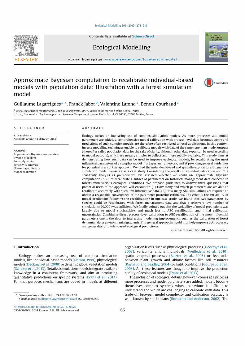
Approximate Bayesian computation to recalibrate individual-basedmodels with population data: Illustration with a forest simulationmodel
Guillaume Lagarrigues a,*, Franck Jabot b, Valentine Lafond a, Benoit Courbaud a
a Irstea, Ecosystèmes Montagnards, 2 rue de la Papeterie, BP 76, 38402 Saint-Martin-d'Hères Cedex, Franceb Irstea, Laboratoire d'Ingénierie pour les Systèmes Complexes, 9 avenue Blaise Pascal, CS 20085, 63178 Aubière, France
A R T I C L E I N F O
Article history:
Available online 13 October 2014
Keywords:
Approximate Bayesian computation
Inverse modeling
Forest dynamics
Sensitivity analysis
Uneven-aged forests
Model calibration
A B S T R A C T
Ecology makes an increasing use of complex simulation models. As more processes and model
parameters are added, a comprehensive model calibration with process-level data becomes costly and
predictions of such complex models are therefore often restricted to local applications. In this context,
inverse modelling techniques enable to calibrate models with data of the same type than model outputs
(thereafter called population data for the sake of clarity, although other data types can be used according
to model outputs), which are usually simpler to collect and more readily available. This study aims at
demonstrating how such data can be used to improve ecological models, by recalibrating the most
influential parameters of a complex model in a Bayesian framework, and at providing general guidelines
for potential users of this approach. We used the individual-based and spatially explicit forest dynamics
simulation model Samsara2 as a case study. Considering the results of an initial calibration and of a
sensitivity analysis as prerequisites, we assessed whether we could use approximate Bayesian
computation (ABC) to recalibrate a subset of parameters on historical management data collected in
forests with various ecological conditions. We propose guidelines to answer three questions that
potential users of the approach will encounter: (1) How many and which parameters are we able to
recalibrate accurately with such low-informative data? (2) How many ABC simulations are required to
obtain a reasonable convergence of the parameter posterior estimates? (3) What is the variability of
model predictions following the recalibration? In our case study, we found that two parameters by
species could be recalibrated with forest management data and that a relatively low number of
simulations (20,000) was sufficient. We finally pointed out that the variability of model predictions was
largely due to model stochasticity, and much less to ABC recalibration and initial calibration
uncertainties. Combining direct process-level calibration to ABC recalibration of the most influential
parameters opens the door to interesting modelling improvements, such as the calibration of forest
dynamics along environmental gradients. This general approach should thus help improve both accuracy
and generality of model-based ecological predictions.
ã 2014 Elsevier B.V. All rights reserved.
1. Introduction
Ecology makes an increasing use of complex simulationmodels, like individual-based models (Grimm, 1999), physiologicalmodels (Deckmyn et al., 2008) or dynamic global vegetationmodels(Scheiteretal., 2013).Detailedsimulationmodels integrate availableknowledge in a consistent framework, and aim at producingquantitative predictions on specific systems (Evans et al., 2013).For that purpose, mechanisms are added in models at different
organization levels, such as physiological processes (Deckmyn et al.,2008), variability among individuals (Vieilledent et al., 2010),spatio-temporal processes (Balzter et al., 1998) or feedbacksbetween plant growth and abiotic factors like soil resources(Raynaud and Leadley, 2004) or light conditions (Courbaud et al.,2003). All these features are thought to improve the predictionquality of ecological models (Evans et al., 2013).
The inclusion of ecological details, however, comes at a price: asmore processes and model parameters are added, models becomethemselves complex systems whose behaviour is difficult tounderstand and which are challenging to calibrate with data. Thistrade-off between model complexity and calibration accuracy iswell-known by statisticians (Burnham and Anderson, 2002). The
* Corresponding author. Tel.: +33 4 76 76 27 07.
E-mail address: [email protected] (G. Lagarrigues).
http://dx.doi.org/10.1016/j.ecolmodel.2014.09.023
0304-3800/ã 2014 Elsevier B.V. All rights reserved.
Ecological Modelling 306 (2015) 278–286
Contents lists available at ScienceDirect
Ecological Modelling
journal homepage: www.elsevier .com/ locate /eco lmodel
66
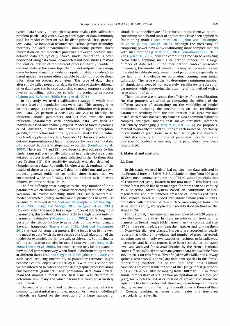
typical data scarcity in ecological systems makes this calibrationproblem particularly acute. Two general types of data commonlyused for model calibration can be distinguished. First, process-level data, like individual resource acquisition, growth, fecundity,mortality or local environmental monitoring provide directinformation on the modelled processes. However, because suchdetailed data are typically scarce, model calibration is oftenperformed using data from unconnected and local studies, makingthe joint calibration of the different processes hardly feasible. Incontrast, data of the same type than model outputs, like canopycover for forest dynamics model or population data for individual-based models, are more often available but do not provide directinformation on process parameters. This type of data (thereafter simply called population data for the sake of clarity, althoughother data types can be used according to model outputs) requiresinverse modelling techniques to infer the ecological processes(Grimm and Railsback, 2005; Hartig et al., 2011).
In this study, we used a calibration strategy in which bothprocess-level and population data were used. This strategy relieson three steps: (1) carry out an initial calibration with process-level data, (2) perform a sensitivity analysis to identify theinfluential model parameters and (3) recalibrate the mostinfluential parameters with population data. We used anindividual-based and spatially explicit model of forest dynamics,called Samsara2, in which the processes of light interception,growth, reproduction andmortality are simulated at the individualtree level (Supplementary data, Appendix A). Thismodel relies on adetailed representation of light interception by tree crowns, takinginto account both stand slope and exposition (Courbaud et al.,2003). The steps (1) and (2) have been carried out prior to thisstudy: Samsara2 was initially calibrated in a restricted area, usingdetailed process-level data mainly collected in the Northern Alps(see Section 2.2); the sensitivity analysis was also detailed in(Supplementary data, Appendix B). After a quick reminder of theresults of these two steps, we will detail the third one and we willpropose general guidelines to tackle three issues that weencountered while performing this recalibration task. In whatfollows, we present these issues.
The first difficulty arose along with the large number of inputparameterswhich commonly characterize complexmodels such asSamsara2. In inverse modelling, modellers usually calibrate allmodel parameters jointly, so that model predictions fit as well aspossible to observed data (Jabot and Bascompte, 2012; Van Oijenet al., 2005; Vrugt and Sadegh, 2013; Wiegand et al., 2003).However, when the model has a large number of interacting inputparameters, this method leads inevitably to a high uncertainty onparameter estimates (Wiegand et al., 2003), or to marginalposterior distributions close to prior distributions when using aBayesian framework (Hartig et al., 2014; Jabot and Bascompte,2012), at least for some parameters. If the focus is on fitting wellthe model to data (with the perspective of a local adaptation of themodel, for example), that is not really problematic. But the finalityof the recalibration can also be model improvement (Dong et al.,2008; Fenicia et al., 2008). For instance, one may be interested inhowmodel parameters vary when fitted in different study sites orat different dates (Foll and Gaggiotti, 2006; Jabot et al., 2008). Insuch cases, reducing uncertainty in parameter estimates mightbecome a central objective. Our study falls within this scope sincewe are interested in calibrating tree demographic processes alongenvironmental gradients using population data from severalmanaged mountain forests. The first issue was therefore todetermine how many and which parameters could be accuratelyrecalibrated.
The second point is linked to the computing time, which iscommonly substantial in complex models. As inverse modellingmethods are based on the repetition of a large number of
simulations, modellers are often reluctant to use themwith time-consuming models and most of applications have been applied tofast-running models (Beaumont, 2010; Jabot and Bascompte,2012; Vrugt and Sadegh, 2013), although the increasing ofcomputing power now allows calibrating more complex modelswith such methods (Hartig et al., 2014; Lenormand et al., 2013;Van Oijen et al., 2005). Still, the computing time can be a limitingfactor when applying such a calibration process on a largenumber of data sets. In the recalibration context presentedpreviously, the number of simulations may be decreased as weintended to calibrate only some model parameters, especially aswe had prior knowledge on parameters coming from initialcalibration. The issue was then to determine a minimum numberof simulations needed to accurately recalibrate a subset ofparameters, while preserving the usability of the method with alarge amount of data.
The third issue was to assess the efficiency of the recalibration.For that purpose, we aimed at comparing the effects of thedifferent sources of uncertainty on the variability of modelpredictions, including the uncertainties on the recalibratedparameters resulting from the recalibration task. Here, we hadto deal withmodel stochasticity, which is also a common feature incomplex ecological models that makes statistical inferenceparticularly challenging (Hartig et al., 2011, 2014). We propose amethod to quantify the contributions of each source of uncertaintyto variability of predictions, so as to disentangle the effects ofmodel stochasticity from those of parameter uncertainties inthis specific context where only some parameters have beenrecalibrated.
2. Material and methods
2.1. Data
In this study, we used historical management data collected inthe Prenovel forest (46.5�N–5.8�E, altitude ranging from 920m to1030m, mean annual temperature of 7.1 �C, annual precipitationof 1700mm per year), located in the Jura massif. This forest is apublic forest which has been managed for more than one centuryas a selection forest system based on continuous naturalregeneration and simultaneous presence of uneven-aged trees.The Prenovel forest is divided into smaller management units,thereafter called stands, with a surface area ranging from 5 to20 ha. In this study, we applied our recalibration method on thestand n� 24.
For this forest, management plans are renewed each 20 years, atso-called inventory years. In these inventories, all trees with adiameter at breast height (dbh) larger than the commercial size(17.5 cm) are recorded, identifying their species and ranking themin 5 cm-wide diameter classes. Harvests are recorded in yearlyreports that indicate the volume and number of trees harvested,grouping species in only two categories: resinous or broadleaves.Inventories and harvest reports have been recorded at the standlevel and archived for several decades by the French NationalForest Office (ONF). Historical management data are available from1953 to 2011 for this forest. Silver fir (Abies alba Mill.) and Norwayspruce (Picea abies (L.) Karst.) are dominant species in this forest,representing together 90% of the total basal area. Climateconditions are comparable to those of the Queige forest (NorthernAlps, 45.7�N–6.5�E, altitude ranging from 1100m to 1550m, meanannual temperature of 5 �C, annual precipitation of 1700mm peryear), for which the initial calibration of growth and allometricequations has been performed. However, mean temperatures areslightly warmer and soil fertility is overall larger in Prenovel thanin Queige, resulting in larger growth rates and tree size,particularly for silver fir.
G. Lagarrigues et al. / Ecological Modelling 306 (2015) 278–286 279
67
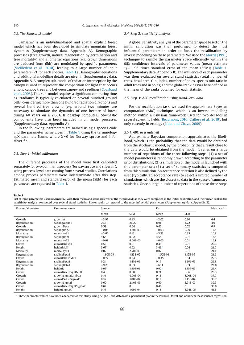
2.2. The Samsara2 model
Samsara2 is an individual-based and spatial explicit forestmodel which has been developed to simulate mountain forestdynamics (Supplementary data, Appendix A). Demographicprocesses (tree growth, natural regeneration by germination andtree mortality) and allometric equations (e.g. crown dimensionsare deduced from dbh) are modulated by specific parameters(Vieilledent et al., 2010), leading to a large number of inputparameters (21 for each species, Table 1). Demographic equationsand additional modelling details are given in Supplementary data,Appendix A. A complex sub-model of radiation interception by thecanopy is used to represent the competition for light that occursamong canopy trees and between canopy and seedlings (Courbaudet al., 2003). This sub-model requires a significant computing timeas irradiance is typically calculated on several hundred groundcells, considering more than one hundred radiation directions andseveral hundred tree crowns (e.g. around two minutes arenecessary to simulate the dynamics of one hectare of forestduring 60 years on a 2.66GHz desktop computer). Stochasticcomponents have also been included in all model processes(Supplementary data, Appendix A).
In the following, parameters are named using a species codeand the parameter name given in Table 1 using the terminologyspX_parameterName, where X = 0 for Norway spruce and 1 forsilver fir.
2.3. Step 1: initial calibration
The different processes of the model were first calibratedseparately for two dominant species (Norway spruce and silver fir),using process-level data coming from several studies. Correlationsamong process parameters were indeterminate after this step.Estimated mean and standard error of the mean (SEM) for eachparameter are reported in Table 1.
2.4. Step 2: sensitivity analysis
A global sensitivity analysis of the parameter space based on theinitial calibration was then performed to detect the mostinfluential parameters in order to focus the recalibration byinversemodelling on these parameters.We used theMorris (1991)technique to sample the parameter space efficiently within the95% confidence intervals of parameter values (mean estimate+/� 1.96 times standard error of the mean (SEM)) (Table 1,Supplementary data, Appendix B). The influence of each parameterwas then evaluated on several stand statistics (total number oftrees, basal area, Gini index, number of poles, species mix ratio inadult trees and in poles) and the global rankingwas here defined asthe mean of the ranks obtained for each statistic.
2.5. Step 3: ABC recalibration using stand-level data
For the recalibration task, we used the approximate Bayesiancomputation (ABC) technique, which is an inverse modellingmethod within a Bayesian framework used for two decades inseveral scientific fields (Beaumont, 2010; Csillery et al., 2010), butonly recently in ecology (Jabot and Chave, 2009).
2.5.1. ABC in a nutshell
Approximate Bayesian computation approximates the likeli-hood, which is the probability that the data would be obtainedfrom the stochastic model, by the probability that a result close tothe data would be obtained from the model. It relies on a largenumber of repetitions of the three following steps: (1) a set ofmodel parameters is randomly drawn according to the parameterprior distributions; (2) a simulation of the model is launched withthis parameter set; (3) a set of summary statistics is computedfrom this simulation. An acceptance criterion is also defined by theuser (typically, an acceptance rate) to select a limited number ofsimulations which are the closest to data in the space of summarystatistics. Once a large number of repetitions of these three steps
Table 1
List of input parameters used in Samsara2, with their mean and standard error of themean (SEM) as they were computed in the initial calibration, and their mean rank in the
sensitivity analysis, computed over several stand statistics. Lower ranks correspond to the most influential parameters (Supplementary data, Appendix B).
Process/allometry Parameter name Spruce Fir Mean rank
Mean SEM Mean SEM
Growth growthA �3.97 0.43 �2.02 0.20 4.4
Regeneration saplingAlpha1 76.81 26.22 8.91 3.72 4.9
Growth growthBeta 0.59 0.04 0.42 0.02 6.9
Regeneration saplingRhg2 �0.05 4.50E-03 �0.03 0.00 15.5
Mortality mortalityP1 �3.60 0.13 �3.21 0.25 16.9
Regeneration saplingRhg1 4.65 0.02 4.55 0.01 18.5
Mortality mortalityP2 �0.01 4.00E-03 �0.03 0.01 19.1
Crown crownRadiusB 0.53 0.01 0.45 0.01 20.3
Height heightMuK 3.67a 0.02 3.43a 0.04 21.0
Mortality mortalityP3 0.02 2.70E-03 0.02 0.01 21.1
Regeneration saplingBeta3 �1.90E-03 1.23E-05 �1.50E-03 1.15E-05 21.6
Crown crownRadiusMuK �0.77 0.04 �0.35 0.04 22.3
Regeneration saplingBeta2 0.24 1.40E-03 0.19 1.26E-03 23.8
Regeneration saplingBeta1 �9.28 0.03 �6.11 0.03 24.8
Height heightR 0.05a 1.50E-03 0.07a 1.55E-03 25.4
Crown crownBaseHeightMuK 0.49 0.08 0.71 0.06 26.3
Growth growthSigmaLambda 0.10 4.00E-04 0.18 8.90E-04 37.9
Crown crownRadiusSigmaK 0.16 1.00E-04 0.12 2.15E-04 38.7
Growth growthSigmaB 0.60 2.40E-03 0.60 2.91E-03 39.3
Crown crownBaseHeightSigmaK 0.62 0 0.46 0 39.8
Height heightSigmaK 0.10 1.00E-04 0.18 8.94E-05 41.3
a These parameter values have been adapated for this study, using height – dbh data from a permanent plot in the Prenovel forest and nonlinear least squares regression.
280 G. Lagarrigues et al. / Ecological Modelling 306 (2015) 278–286
68
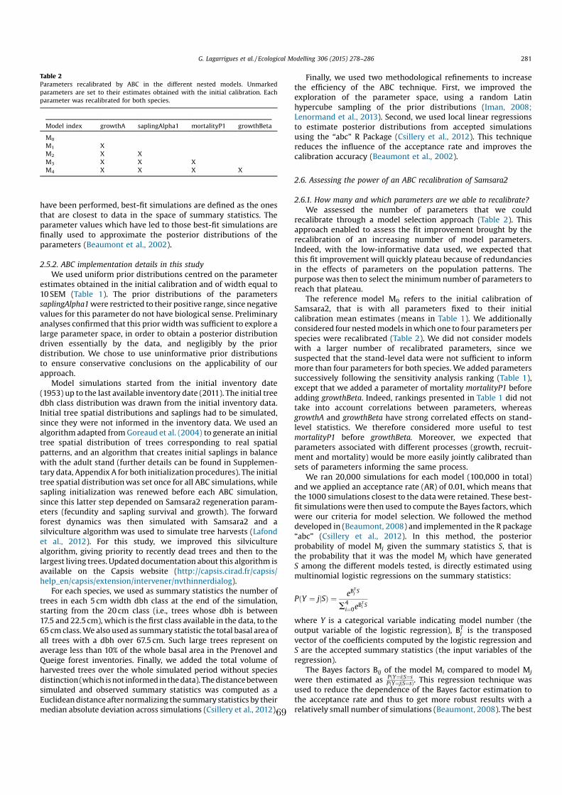
have been performed, best-fit simulations are defined as the onesthat are closest to data in the space of summary statistics. Theparameter values which have led to those best-fit simulations arefinally used to approximate the posterior distributions of theparameters (Beaumont et al., 2002).
2.5.2. ABC implementation details in this study
We used uniform prior distributions centred on the parameterestimates obtained in the initial calibration and of width equal to10SEM (Table 1). The prior distributions of the parameterssaplingAlpha1were restricted to their positive range, since negativevalues for this parameter do not have biological sense. Preliminaryanalyses confirmed that this prior widthwas sufficient to explore alarge parameter space, in order to obtain a posterior distributiondriven essentially by the data, and negligibly by the priordistribution. We chose to use uninformative prior distributionsto ensure conservative conclusions on the applicability of ourapproach.
Model simulations started from the initial inventory date(1953) up to the last available inventory date (2011). The initial treedbh class distribution was drawn from the initial inventory data.Initial tree spatial distributions and saplings had to be simulated,since they were not informed in the inventory data. We used analgorithm adapted fromGoreaud et al. (2004) to generate an initialtree spatial distribution of trees corresponding to real spatialpatterns, and an algorithm that creates initial saplings in balancewith the adult stand (further details can be found in Supplemen-tary data, Appendix A for both initializationprocedures). The initialtree spatial distributionwas set once for all ABC simulations, whilesapling initialization was renewed before each ABC simulation,since this latter step depended on Samsara2 regeneration param-eters (fecundity and sapling survival and growth). The forwardforest dynamics was then simulated with Samsara2 and asilviculture algorithm was used to simulate tree harvests (Lafondet al., 2012). For this study, we improved this silviculturealgorithm, giving priority to recently dead trees and then to thelargest living trees. Updated documentation about this algorithm isavailable on the Capsis website (http://capsis.cirad.fr/capsis/help_en/capsis/extension/intervener/nvthinnerdialog).
For each species, we used as summary statistics the number oftrees in each 5 cm width dbh class at the end of the simulation,starting from the 20cm class (i.e., trees whose dbh is between17.5 and 22.5 cm), which is the first class available in the data, to the65cmclass.We also used as summary statistic the total basal area ofall trees with a dbh over 67.5 cm. Such large trees represent onaverage less than 10% of the whole basal area in the Prenovel andQueige forest inventories. Finally, we added the total volume ofharvested trees over the whole simulated period without speciesdistinction(which isnot informed inthedata). Thedistancebetweensimulated and observed summary statistics was computed as aEuclideandistanceafter normalizing the summarystatistics by theirmedian absolute deviation across simulations (Csillery et al., 2012).
Finally, we used two methodological refinements to increasethe efficiency of the ABC technique. First, we improved theexploration of the parameter space, using a random Latinhypercube sampling of the prior distributions (Iman, 2008;Lenormand et al., 2013). Second, we used local linear regressionsto estimate posterior distributions from accepted simulationsusing the “abc” R Package (Csillery et al., 2012). This techniquereduces the influence of the acceptance rate and improves thecalibration accuracy (Beaumont et al., 2002).
2.6. Assessing the power of an ABC recalibration of Samsara2
2.6.1. How many and which parameters are we able to recalibrate?
We assessed the number of parameters that we couldrecalibrate through a model selection approach (Table 2). Thisapproach enabled to assess the fit improvement brought by therecalibration of an increasing number of model parameters.Indeed, with the low-informative data used, we expected thatthis fit improvement will quickly plateau because of redundanciesin the effects of parameters on the population patterns. Thepurpose was then to select the minimum number of parameters toreach that plateau.
The reference model M0 refers to the initial calibration ofSamsara2, that is with all parameters fixed to their initialcalibration mean estimates (means in Table 1). We additionallyconsidered four nestedmodels inwhich one to four parameters perspecies were recalibrated (Table 2). We did not consider modelswith a larger number of recalibrated parameters, since wesuspected that the stand-level data were not sufficient to informmore than four parameters for both species. We added parameterssuccessively following the sensitivity analysis ranking (Table 1),except that we added a parameter of mortality mortalityP1 beforeadding growthBeta. Indeed, rankings presented in Table 1 did nottake into account correlations between parameters, whereasgrowthA and growthBeta have strong correlated effects on stand-level statistics. We therefore considered more useful to testmortalityP1 before growthBeta. Moreover, we expected thatparameters associated with different processes (growth, recruit-ment and mortality) would be more easily jointly calibrated thansets of parameters informing the same process.
We ran 20,000 simulations for each model (100,000 in total)and we applied an acceptance rate (AR) of 0.01, which means thatthe 1000 simulations closest to the datawere retained. These best-fit simulations were then used to compute the Bayes factors, whichwere our criteria for model selection. We followed the methoddeveloped in (Beaumont, 2008) and implemented in the R package“abc” (Csillery et al., 2012). In this method, the posteriorprobability of model Mj given the summary statistics S, that isthe probability that it was the model Mj which have generatedS among the different models tested, is directly estimated usingmultinomial logistic regressions on the summary statistics:
PðY ¼ jjSÞ ¼eB
Tj S
S4i¼0e
BTi S
where Y is a categorical variable indicating model number (theoutput variable of the logistic regression), BT
j is the transposedvector of the coefficients computed by the logistic regression andS are the accepted summary statistics (the input variables of theregression).
The Bayes factors Bij of the model Mi compared to model Mj
were then estimated as PðY¼ijS¼sPðY¼jjS¼sÞ. This regression technique was
used to reduce the dependence of the Bayes factor estimation tothe acceptance rate and thus to get more robust results with arelatively small number of simulations (Beaumont, 2008). The best
Table 2
Parameters recalibrated by ABC in the different nested models. Unmarked
parameters are set to their estimates obtained with the initial calibration. Each
parameter was recalibrated for both species.
Model index growthA saplingAlpha1 mortalityP1 growthBeta
M0
M1 X
M2 X X
M3 X X X
M4 X X X X
G. Lagarrigues et al. / Ecological Modelling 306 (2015) 278–286 281
69
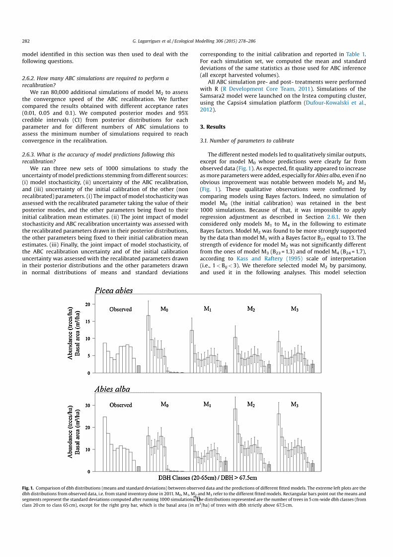
model identified in this section was then used to deal with thefollowing questions.
2.6.2. How many ABC simulations are required to perform a
recalibration?
We ran 80,000 additional simulations of model M2 to assessthe convergence speed of the ABC recalibration. We furthercompared the results obtained with different acceptance rates(0.01, 0.05 and 0.1). We computed posterior modes and 95%credible intervals (CI) from posterior distributions for eachparameter and for different numbers of ABC simulations toassess the minimum number of simulations required to reachconvergence in the recalibration.
2.6.3. What is the accuracy of model predictions following this
recalibration?
We ran three new sets of 1000 simulations to study theuncertainty ofmodel predictions stemming fromdifferent sources:(i) model stochasticity, (ii) uncertainty of the ABC recalibration,and (iii) uncertainty of the initial calibration of the other (nonrecalibrated) parameters. (i) The impact ofmodel stochasticitywasassessed with the recalibrated parameter taking the value of theirposterior modes, and the other parameters being fixed to theirinitial calibration mean estimates. (ii) The joint impact of modelstochasticity and ABC recalibration uncertainty was assessed withthe recalibrated parameters drawn in their posterior distributions,the other parameters being fixed to their initial calibration meanestimates. (iii) Finally, the joint impact of model stochasticity, ofthe ABC recalibration uncertainty and of the initial calibrationuncertainty was assessed with the recalibrated parameters drawnin their posterior distributions and the other parameters drawnin normal distributions of means and standard deviations
corresponding to the initial calibration and reported in Table 1.For each simulation set, we computed the mean and standarddeviations of the same statistics as those used for ABC inference(all except harvested volumes).
All ABC simulation pre- and post- treatments were performedwith R (R Development Core Team, 2011). Simulations of theSamsara2 model were launched on the Irstea computing cluster,using the Capsis4 simulation platform (Dufour-Kowalski et al.,2012).
3. Results
3.1. Number of parameters to calibrate
The different nestedmodels led to qualitatively similar outputs,except for model M0 whose predictions were clearly far fromobserved data (Fig. 1). As expected, fit quality appeared to increaseasmore parameterswere added, especially for Abies alba, even if noobvious improvement was notable between models M2 and M3
(Fig. 1). These qualitative observations were confirmed bycomparing models using Bayes factors. Indeed, no simulation ofmodel M0 (the initial calibration) was retained in the best1000 simulations. Because of that, it was impossible to applyregression adjustment as described in Section 2.6.1. We thenconsidered only models M1 to M4 in the following to estimateBayes factors. Model M2 was found to be more strongly supportedby the data than model M1 with a Bayes factor B21 equal to 13. Thestrength of evidence for model M2 was not significantly differentfrom the ones of model M3 (B23 =1.3) and of model M4 (B24= 1.7),according to Kass and Raftery (1995) scale of interpretation(i.e., 1<Bij<3). We therefore selected model M2 by parsimony,and used it in the following analyses. This model selection
[(Fig._1)TD$FIG]
Fig. 1. Comparison of dbh distributions (means and standard deviations) between observed data and the predictions of different fittedmodels. The extreme left plots are the
dbh distributions from observed data, i.e. from stand inventory done in 2011. M0, M1, M2 andM3 refer to the different fittedmodels. Rectangular bars point out themeans and
segments represent the standard deviations computed after running 1000 simulations. The distributions represented are the number of trees in 5 cm-wide dbh classes (from
class 20 cm to class 65 cm), except for the right grey bar, which is the basal area (in m2/ha) of trees with dbh strictly above 67,5 cm.
282 G. Lagarrigues et al. / Ecological Modelling 306 (2015) 278–286
70
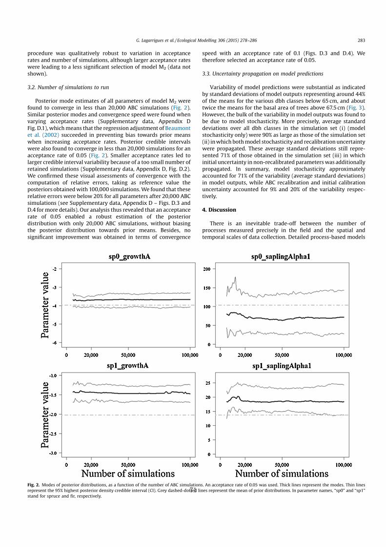
procedure was qualitatively robust to variation in acceptancerates and number of simulations, although larger acceptance rateswere leading to a less significant selection of model M2 (data notshown).
3.2. Number of simulations to run
Posterior mode estimates of all parameters of model M2 werefound to converge in less than 20,000 ABC simulations (Fig. 2).Similar posterior modes and convergence speed were found whenvarying acceptance rates (Supplementary data, Appendix DFig. D.1), whichmeans that the regression adjustment of Beaumontet al. (2002) succeeded in preventing bias towards prior meanswhen increasing acceptance rates. Posterior credible intervalswere also found to converge in less than 20,000 simulations for anacceptance rate of 0.05 (Fig. 2). Smaller acceptance rates led tolarger credible interval variability because of a too small number ofretained simulations (Supplementary data, Appendix D, Fig. D.2).We confirmed these visual assessments of convergence with thecomputation of relative errors, taking as reference value theposteriors obtainedwith 100,000 simulations.We found that theserelative errors were below 20% for all parameters after 20,000 ABCsimulations (see Supplementary data, Appendix D – Figs. D.3 andD.4 formore details). Our analysis thus revealed that an acceptancerate of 0.05 enabled a robust estimation of the posteriordistribution with only 20,000 ABC simulations, without biasingthe posterior distribution towards prior means. Besides, nosignificant improvement was obtained in terms of convergence
speed with an acceptance rate of 0.1 (Figs. D.3 and D.4). Wetherefore selected an acceptance rate of 0.05.
3.3. Uncertainty propagation on model predictions
Variability of model predictions were substantial as indicatedby standard deviations of model outputs representing around 44%of the means for the various dbh classes below 65 cm, and abouttwice the means for the basal area of trees above 67.5 cm (Fig. 3).However, the bulk of the variability in model outputs was found tobe due to model stochasticity. More precisely, average standarddeviations over all dbh classes in the simulation set (i) (modelstochasticity only) were 90% as large as those of the simulation set(ii) inwhich bothmodel stochasticity and recalibration uncertaintywere propagated. These average standard deviations still repre-sented 71% of those obtained in the simulation set (iii) in whichinitial uncertainty in non-recalibrated parameterswas additionallypropagated. In summary, model stochasticity approximatelyaccounted for 71% of the variability (average standard deviations)in model outputs, while ABC recalibration and initial calibrationuncertainty accounted for 9% and 20% of the variability respec-tively.
4. Discussion
There is an inevitable trade-off between the number ofprocesses measured precisely in the field and the spatial andtemporal scales of data collection. Detailed process-based models
[(Fig._2)TD$FIG]
Fig. 2. Modes of posterior distributions, as a function of the number of ABC simulations. An acceptance rate of 0.05 was used. Thick lines represent the modes. Thin lines
represent the 95% highest posterior density credible interval (CI). Grey dashed-dotted lines represent the mean of prior distributions. In parameter names, “sp0” and “sp1”
stand for spruce and fir, respectively.
G. Lagarrigues et al. / Ecological Modelling 306 (2015) 278–286 283
71
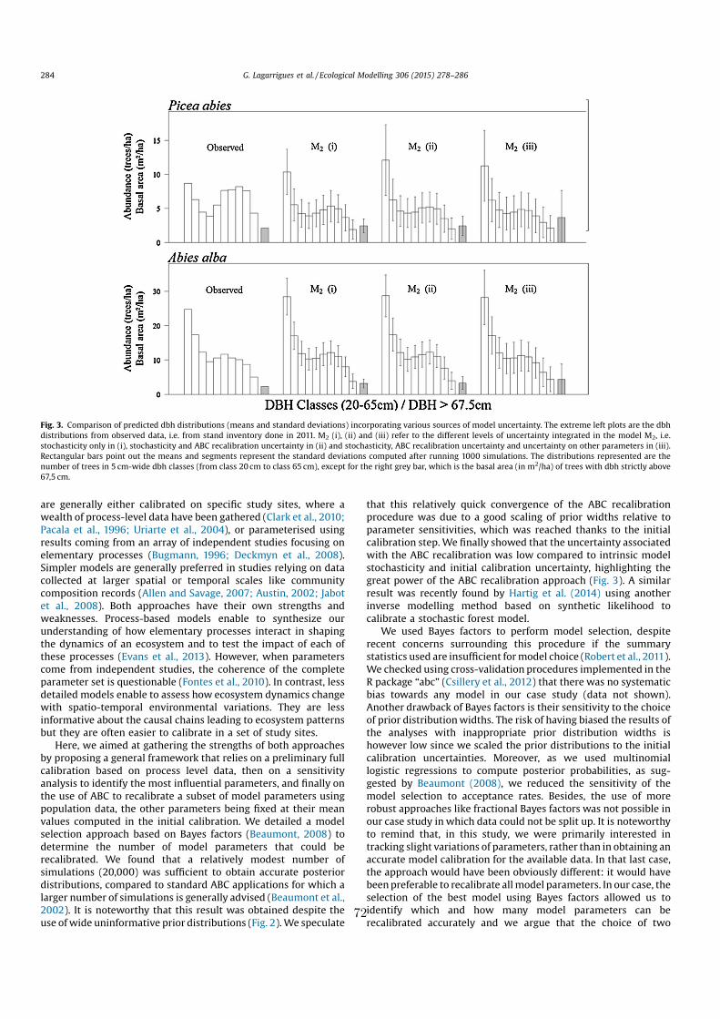
are generally either calibrated on specific study sites, where awealth of process-level data have been gathered (Clark et al., 2010;Pacala et al., 1996; Uriarte et al., 2004), or parameterised usingresults coming from an array of independent studies focusing onelementary processes (Bugmann, 1996; Deckmyn et al., 2008).Simpler models are generally preferred in studies relying on datacollected at larger spatial or temporal scales like communitycomposition records (Allen and Savage, 2007; Austin, 2002; Jabotet al., 2008). Both approaches have their own strengths andweaknesses. Process-based models enable to synthesize ourunderstanding of how elementary processes interact in shapingthe dynamics of an ecosystem and to test the impact of each ofthese processes (Evans et al., 2013). However, when parameterscome from independent studies, the coherence of the completeparameter set is questionable (Fontes et al., 2010). In contrast, lessdetailed models enable to assess how ecosystem dynamics changewith spatio-temporal environmental variations. They are lessinformative about the causal chains leading to ecosystem patternsbut they are often easier to calibrate in a set of study sites.
Here, we aimed at gathering the strengths of both approachesby proposing a general framework that relies on a preliminary fullcalibration based on process level data, then on a sensitivityanalysis to identify the most influential parameters, and finally onthe use of ABC to recalibrate a subset of model parameters usingpopulation data, the other parameters being fixed at their meanvalues computed in the initial calibration. We detailed a modelselection approach based on Bayes factors (Beaumont, 2008) todetermine the number of model parameters that could berecalibrated. We found that a relatively modest number ofsimulations (20,000) was sufficient to obtain accurate posteriordistributions, compared to standard ABC applications for which alarger number of simulations is generally advised (Beaumont et al.,2002). It is noteworthy that this result was obtained despite theuse ofwide uninformative prior distributions (Fig. 2).We speculate
that this relatively quick convergence of the ABC recalibrationprocedure was due to a good scaling of prior widths relative toparameter sensitivities, which was reached thanks to the initialcalibration step.We finally showed that the uncertainty associatedwith the ABC recalibration was low compared to intrinsic modelstochasticity and initial calibration uncertainty, highlighting thegreat power of the ABC recalibration approach (Fig. 3). A similarresult was recently found by Hartig et al. (2014) using anotherinverse modelling method based on synthetic likelihood tocalibrate a stochastic forest model.
We used Bayes factors to perform model selection, despiterecent concerns surrounding this procedure if the summarystatistics used are insufficient formodel choice (Robert et al., 2011).We checked using cross-validation procedures implemented in theR package “abc” (Csillery et al., 2012) that there was no systematicbias towards any model in our case study (data not shown).Another drawback of Bayes factors is their sensitivity to the choiceof prior distributionwidths. The risk of having biased the results ofthe analyses with inappropriate prior distribution widths ishowever low since we scaled the prior distributions to the initialcalibration uncertainties. Moreover, as we used multinomiallogistic regressions to compute posterior probabilities, as sug-gested by Beaumont (2008), we reduced the sensitivity of themodel selection to acceptance rates. Besides, the use of morerobust approaches like fractional Bayes factors was not possible inour case study in which data could not be split up. It is noteworthyto remind that, in this study, we were primarily interested intracking slight variations of parameters, rather than in obtaining anaccurate model calibration for the available data. In that last case,the approach would have been obviously different: it would havebeenpreferable to recalibrate allmodel parameters. In our case, theselection of the best model using Bayes factors allowed us toidentify which and how many model parameters can berecalibrated accurately and we argue that the choice of two
[(Fig._3)TD$FIG]
Fig. 3. Comparison of predicted dbh distributions (means and standard deviations) incorporating various sources of model uncertainty. The extreme left plots are the dbh
distributions from observed data, i.e. from stand inventory done in 2011. M2 (i), (ii) and (iii) refer to the different levels of uncertainty integrated in the model M2, i.e.
stochasticity only in (i), stochasticity and ABC recalibration uncertainty in (ii) and stochasticity, ABC recalibration uncertainty and uncertainty on other parameters in (iii).
Rectangular bars point out the means and segments represent the standard deviations computed after running 1000 simulations. The distributions represented are the
number of trees in 5 cm-wide dbh classes (from class 20 cm to class 65 cm), except for the right grey bar, which is the basal area (in m2/ha) of trees with dbh strictly above
67,5 cm.
284 G. Lagarrigues et al. / Ecological Modelling 306 (2015) 278–286
72
parameters by species was optimal, given our low-informativedata and our purpose.
Only standard ABC methods (with regression adjustments)were applied in this study whereas other methods are available touse more efficient sampling techniques, such as sequential orcoupled-to-MCMC algorithms (Jabot et al., 2013; Marin et al.,2012). We made this choice because we wanted to assess theconvergence speed of the ABC recalibration and to perform modelselection.We advise to use such a standard ABC sampling approachwhen developing an ABC recalibration procedure for new pairs ofmodel and data type, and to only use more efficient algorithms forsubsequent recalibrations of the same model with new data of thesame type. The use of these improved techniques may enable toreach up to one order of magnitude of computing speed increase(Lenormand et al., 2013). These additional computing savings mayfurther broaden the applicability of the methodology proposedhere, for instance by allowing its use on a large number of foreststands.
ABC recalibration opens the door for large scale fit ofmechanistic ecological models. Inferring model parameters usinglow-informative data from multiple sources was recently recog-nized as a pertinent and complementary approach to directparameterization (Hartig et al., 2012). For instance, in our case,we could use this method to track the effects of environmentalgradients on forest dynamics. Tree ring analyses are commonlyused to explore such correlations between tree growth andclimate conditions like temperature and precipitation (Battipagliaet al., 2009; Carrer et al., 2012). The inverse modelling approachpresented in this study allows taking into account the effects oftree harvests, and stand conditions (basal area, tree sizedistributions) in a mechanistic framework, whereas these latterfactors must generally be considered as control variables in treering analyses. Moreover, even with heavy restrictions on thenumber of parameters to calibrate, we were able to accuratelycalibrate two key demographic processes driving uneven-agedforest dynamics, in particular natural regeneration which is oftenpoorly considered in forest models and yet a very importantdriver of uneven-aged forests (Bugmann, 2001; Schütz, 1997). Weexpect that ABC recalibration could enable to disentangle theeffects of harvests from those of abiotic factors on tree sizedistributions in managed spruce-fir forests. This should helpproposing adjustments to adapt forest management to environ-mental changes. More generally, the approach proposed hereshould help to scale up the detailed local understanding of manyecological systems to regional and continental scales, byproviding a platform to integrate several complementary datasources in a unified calibration framework.
5. Conclusion
The use of inverse modelling techniques with complexecological models has been mainly used to adapt the model tospecific conditions, by recalibrating all model parameters.We havedemonstrated here that approximate Bayesian computationenables also to track fine variations of a small number of modelparameters using population data and an initial model calibrationbased on process-level data. By integrating data collected atdifferent organization levels in a Bayesian calibration, the methodproposed here may improve both accuracy and generality ofecological model predictions.
Acknowledgments
We thank Nicolas Dumoulin, François de Coligny and VincentChevallereau for their help during the course of this study. Wealso thank Anne-Lise Bartalucci, who gathered the inventory and
management records for the Prenovel forest. GuillaumeLagarrigues was funded by the French Environment and EnergyManagement Agency (ADEME) and the French Forest NationalOffice (ONF), and by a grant from Irstea. Valentine Lafond wasfunded by the GeForHet project (n� E23/2010), from the Frenchresearch program “Biodiversity, Forest Management and PublicPolicy” (BGF).
Appendix A. Supplementary data
Supplementary data associated with this article can befound, in the online version, at http://dx.doi.org/10.1016/j.ecolmo-del.2014.09.023.
References
Allen, A.P., Savage, V.M., 2007. Setting the absolute tempo of biodiversity dynamics.Ecol. Lett. 10, 637–646.
Austin, M.P., 2002. Spatial prediction of species distribution: an interface betweenecological theory and statistical modelling. Ecol. Model. 157, 101–118.
Balzter, H., Braun, P.W., Kohler, W., 1998. Cellular automata models for vegetationdynamics. Ecol. Model. 107, 113–125.
Battipaglia, G., Saurer, M., Cherubini, P., Siegwolf, R.T.W., Cotrufo, M.F., 2009. Treerings indicate different drought resistance of a native (Abies alba Mill.) and anonnative (Picea abies (L.) Karst.) species co-occurring at a dry site in SouthernItaly. Forest Ecol. Manag. 257, 820–828.
Beaumont, M.A., 2008. Joint determination of topology, divergence time, andimmigration inpopulation trees. In: Renfrew, C.,Matsumura, S., Forster, P. (Eds.),Simulation, Genetics and Human Prehistory. McDonald Institute Monographs,pp. 134–1541.
Beaumont, M.A., 2010. Approximate Bayesian computation in evolution andecology. In: Futuyma, D.J., Shafer, H.B., Simberloff, D. (Eds.), Annual Review ofEcology, Evolution, and Systematics, Vol. 41. , pp. 379–406.
Beaumont, M.A., Zhang, W.Y., Balding, D.J., 2002. Approximate Bayesian computa-tion in population genetics. Genetics 162, 2025–2035.
Bugmann, H., 2001. A review of forest gap models. Climatic Change 51, 259–305.Bugmann, H.K., 1996. A simplified forest model to study species composition along
climate gradients. Ecology 77, 2055–2074.Burnham, K.P., Anderson, D.R., 2002. Model selection and multi-model inference: a
practical information-theoretic approach. Springer .Carrer, M., Motta, R., Nola, P., 2012. Significantmean and extreme climate sensitivity
of Norway spruce and silver fir at mid-elevation mesic sites in the Alps. PLoSOne 7 (11), e50755. doi:http://dx.doi.org/10.1371/journal.pone.0050755.
Clark, J.S., Bell, D., Chu, C., Courbaud, B., Dietze, M., Hersh, M., et al., 2010. High-dimensional coexistence based on individual variation: a synthesis of evidence.Ecol. Monogr. 80, 569–608.
Courbaud, B., deColigny, F., Cordonnier, T., 2003. Simulating radiation distribution in aheterogeneous Norway spruce forest on a slope. Agric. ForestMeteorol.116,1–18.
Csillery, K., Blum, M.G.B., Gaggiotti, O.E., Francois, O., 2010. Approximate Bayesiancomputation (ABC) in practice. Trends Ecol. Evol. 25, 410–418.
Csillery, K., Francois, O., Blum, M.G.B., 2012. abc: an R package for approximateBayesian computation (ABC). Methods Ecol. Evol. 3, 475–479.
Deckmyn, G., Verbeeck, H., Op de Beeck, M., Vansteenkiste, D., Steppe, K.,Ceulemans, R., 2008. ANAFORE: a stand-scale process-based forest model thatincludes wood tissue development and labile carbon storage in trees. Ecol.Model. 215, 345–368.
Dong, Q., Louarn, G., Wang, Y., Barczi, J.-F., De Reffye, P., 2008. Does the structure–function model GREENLAB deal with crop phenotypic plasticity induced byplant spacing? A case study on tomato. Ann. Bot. 101, 1195–1206.
Dufour-Kowalski, S., Courbaud, B., Dreyfus, P., Meredieu, C., de Coligny, F., 2012.Capsis: an open software framework and community for forest growthmodelling. Ann. For. Sci. 69, 221–233.
Evans, M.R., Grimm, V., Johst, K., Knuuttila, T., de Langhe, R., Lessells, C.M., et al.,2013. Do simple models lead to generality in ecology? Trends Ecol. Evol. 28,578–583.
Fenicia, F., McDonnell, J.J., Savenije, H.H.G., 2008. Learning from model improve-ment: on the contribution of complementary data to process understanding.Water Resour. Res. 44.
Foll, M., Gaggiotti, O., 2006. Identifying the environmental factors that determinethe genetic structure of populations. Genetics 174, 875–891.
Fontes, L., Bontemps, J.D., Bugmann, H., Van Oijen, M., Gracia, C., Kramer, K., et al.,2010. Models for supporting forest management in a changing environment.Forest Syst. 19, 8–29.
Goreaud, F., Loussier, B., Ngo Bieng,M.A., Allain, R., 2004. Simulating Realistic SpatialStructure for Forest Stands: A Mimetic Point Process. Interdisciplinary SpatialStatistics Workshop, Paris, pp. 22.
Grimm, V., 1999. Ten years of individual-based modelling in ecology: what have welearned and what could we learn in the future? Ecol. Model. 115, 129–148.
Grimm, V., Railsback, S.F., 2005. Individual-based Modeling and Ecology. PrincetonUniversity Press, pp. 428.
G. Lagarrigues et al. / Ecological Modelling 306 (2015) 278–286 285
73
Hartig, F., Calabrese, J.M., Reineking, B., Wiegand, T., Huth, A., 2011. Statisticalinference for stochastic simulation models – theory and application. Ecol. Lett.14, 816–827.
Hartig, F., Dislich, C., Wiegand, T., Huth, A., 2014. Technical note: approximateBayesian parameterization of a process-based tropical forest model. Biogeo-sciences 11, 1261–1272.
Hartig, F., Dyke, J., Hickler, T., Higgins, S.I., O'Hara, R.B., Scheiter, S., et al., 2012.Connecting dynamic vegetation models to data – an inverse perspective. J.Biogeogr. 39, 2240–2252.
Iman, R.L., 2008. Latin hypercube sampling. Encyclopedia of Quantitative RiskAnalysis and Assessment. John Wiley & Sons Ltd.
Jabot, F., Bascompte, J., 2012. Bitrophic interactions shape biodiversity in space. Proc.Natl. Acad. Sci. U. S. A. 109, 4521–4526.
Jabot, F., Chave, J., 2009. Inferring the parameters of the neutral theory ofbiodiversity using phylogenetic information and implications for tropicalforests. Ecol. Lett. 12, 239–248.
Jabot, F., Etienne, R.S., Chave, J., 2008. Reconciling neutral community models andenvironmental filtering: theory and an empirical test. Oikos 117, 1308–1320.
Jabot, F., Faure, T., Dumoulin, N., 2013. Easy ABC: performing efficient approximateBayesian computation sampling schemes using R. Methods Ecol. Evol. 4,684–687.
Kass, R.E., Raftery, A.E., 1995. Bayes factors. J. Am. Stat. Assoc. 90, 773–795.Lafond, V., Cordonnier, T., De Coligny, F., Courbaud, B., 2012. Reconstructing
harvesting diameter distribution from aggregate data. Ann. Forest Sci. 69,235–243.
Lenormand, M., Jabot, F., Deffuant, G., 2013. Adaptive approximate Bayesiancomputation for complex models. Comput. Stat. 28, 2777–2796.
Marin, J.-M., Pudlo, P., Robert, C.P., Ryder, R.J., 2012. Approximate Bayesiancomputational methods. Stat. Comput. 22, 1167–1180.
Morris, M.D., 1991. Factorial sampling plans for preliminary computationalexperiments. Technometrics 33, 161–174.
Pacala, S.W., Canham, C.D., Saponara, J., Silander, J.A., Kobe, R.K., Ribbens, E., 1996.Forest models defined by field measurements: estimation, error analysis anddynamics. Ecol. Monogr. 66, 1–43.
R. Development Core Team, 2011. A Language and Environment for StatisticalComputing. R Foundation for Statistical Computing, Vienna, Austria.
Raynaud, X., Leadley, P.W., 2004. Soil characteristics play a key role inmodeling nutrient competition in plant communities. Ecology 85,2200–2214.
Robert, C.P., Cornuet, J.-M., Marin, J.-M., Pillai, N.S., 2011. Lack of confidence inapproximate Bayesian computation model choice. Proc. Natl. Acad. Sci. U. S. A.108, 15112–15117.
Scheiter, S., Langan, L., Higgins, S.I., 2013. Next-generation dynamic globalvegetation models: learning from community ecology. New Phytol. 198,957–969.
Schütz, 1997. Sylviculture 2: La gestion des forêts irrégulières et mélangées. Pressespolytechniques et universitaires romandes, p. 178.
Uriarte, M., Condit, R., Canham, C.D., Hubbell, S.P., 2004. A spatially explicit model ofsapling growth in a tropical forest: does the identity of neighbours matter? J.Ecol. 92, 348–360.
Van Oijen, M., Rougier, J., Smith, R., 2005. Bayesian calibration of process-basedforest models: bridging the gap between models and data. Tree Physiol. 25,915–927.
Vieilledent, G., Courbaud, B., Kunstler, G., Dhote, J.F., Clark, J.S., 2010. Individualvariability in tree allometry determines light resource allocation inforest ecosystems: a hierarchical Bayesian approach. Oecologia 163,759–773.
Vrugt, J.A., Sadegh, M., 2013. Toward diagnostic model calibration and evaluation:approximate Bayesian computation. Water Resour. Res. 49, 4335–4345.
Wiegand, T., Jeltsch, F., Hanski, I., Grimm, V., 2003. Using pattern-orientedmodelingfor revealing hidden information: a key for reconciling ecological theory andapplication. Oikos 100, 209–222.
286 G. Lagarrigues et al. / Ecological Modelling 306 (2015) 278–286
74
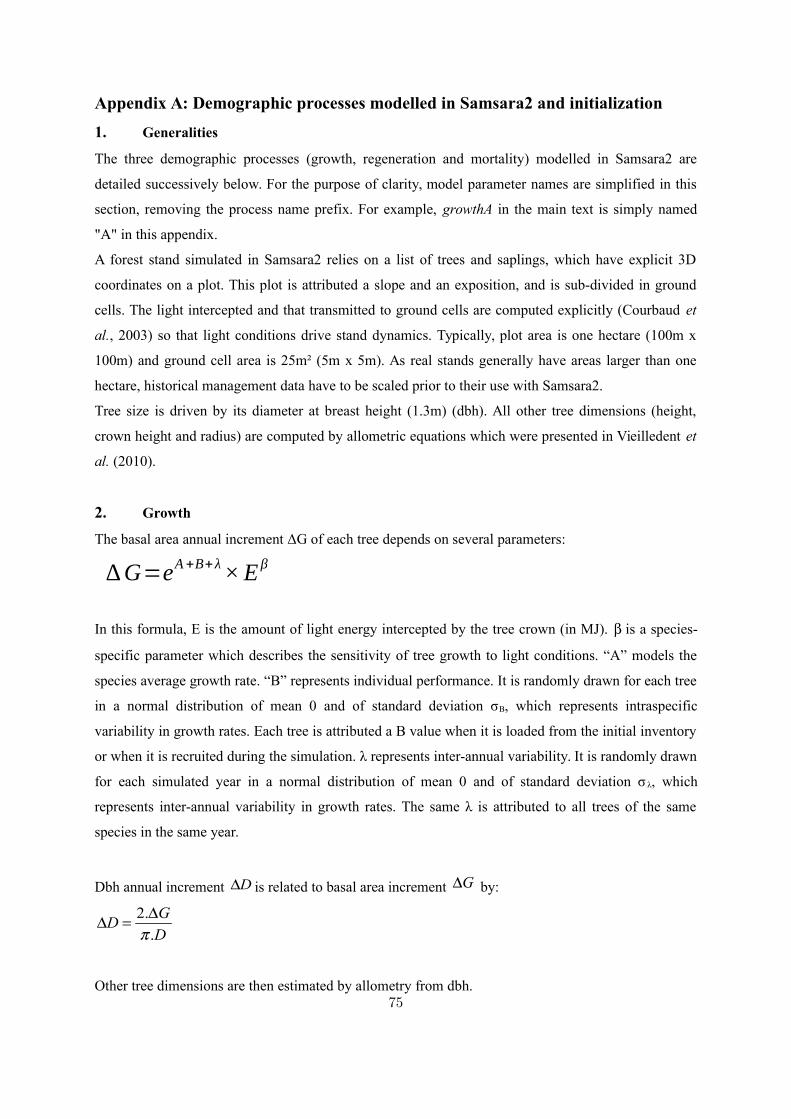
Appendix A: Demographic processes modelled in Samsara2 and initialization
1. Generalities
The three demographic processes (growth, regeneration and mortality) modelled in Samsara2 are
detailed successively below. For the purpose of clarity, model parameter names are simplified in this
section, removing the process name prefix. For example, growthA in the main text is simply named
"A" in this appendix.
A forest stand simulated in Samsara2 relies on a list of trees and saplings, which have explicit 3D
coordinates on a plot. This plot is attributed a slope and an exposition, and is sub-divided in ground
cells. The light intercepted and that transmitted to ground cells are computed explicitly (Courbaud et
al., 2003) so that light conditions drive stand dynamics. Typically, plot area is one hectare (100m x
100m) and ground cell area is 25m² (5m x 5m). As real stands generally have areas larger than one
hectare, historical management data have to be scaled prior to their use with Samsara2.
Tree size is driven by its diameter at breast height (1.3m) (dbh). All other tree dimensions (height,
crown height and radius) are computed by allometric equations which were presented in Vieilledent et
al. (2010).
2. Growth
The basal area annual increment ΔG of each tree depends on several parameters:
∆G=eA+B+λ
×Eβ
In this formula, E is the amount of light energy intercepted by the tree crown (in MJ). β is a species-
specific parameter which describes the sensitivity of tree growth to light conditions. “A” models the
species average growth rate. “B” represents individual performance. It is randomly drawn for each tree
in a normal distribution of mean 0 and of standard deviation σB, which represents intraspecific
variability in growth rates. Each tree is attributed a B value when it is loaded from the initial inventory
or when it is recruited during the simulation. λ represents inter-annual variability. It is randomly drawn
for each simulated year in a normal distribution of mean 0 and of standard deviation σ λ, which
represents inter-annual variability in growth rates. The same λ is attributed to all trees of the same
species in the same year.
Dbh annual increment D∆ is related to basal area increment G∆ by:
2.
.
GD
Dπ
∆∆ =
Other tree dimensions are then estimated by allometry from dbh.75

3. Regeneration
Natural regeneration is composed of several sub-processes described below: sapling installation,
sapling growth and tree recruitment (= end of sapling stage).
3.1 Sapling installation
Numbers of installed saplings are computed in each ground cell by independent Poisson draws of
mean α1 × BA × S where α1 is a species-specific recruitment rate, BA is the basal area of conspecific
trees located within 25m of the focal grid cell, and S is a sapling survival probability given by:
S=1
1+e−(β
1+β
2×L+β
3×L²)
where β1, β2 and β3 are model parameters and L is the proportion of light (expressed as the percentage
of light available above the canopy) reaching the ground cell.
The coordinates of each sapling within the ground cell are drawn in uniform distributions.
3.2 Sapling growth
Installed saplings are described by their height, which annual increment ΔH is given by:
∆ H=H ×(1−1
100×e
Rhg1+Rhg
2× ln (L))
where H is current sapling height, Rhg1 is the species-specific sapling growth rate and Rhg2 is the
dependency to cell light conditions (L) of sapling growth.
3.3 Tree recruitment
When saplings reach a recruitment height of 3.8m for Picea abies and of 4.6m for Abies alba, they are
recruited as trees in the stand. These recruitment heights correspond to a dbh of 7.5cm (which is the
minimal dbh recorded in adult tree data).
4. Mortality
Each year, trees die with probability M given by:
M=1−(1−m)0.2
where m is a mortality probability over 5 years-long time periods.
m=max (m1 ,m2 )
76
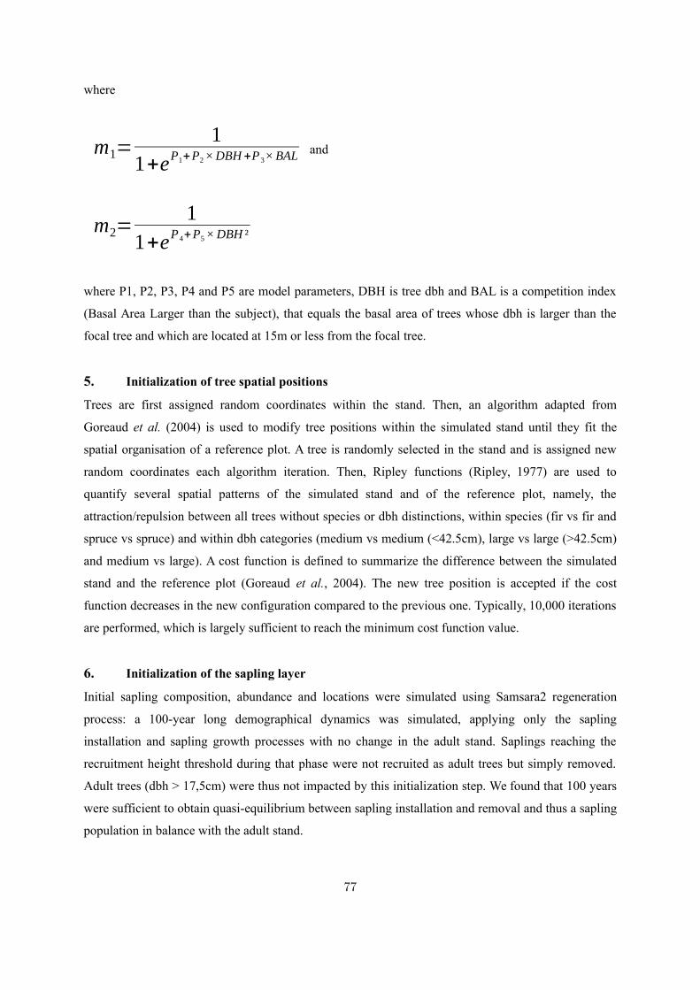
where
m1=1
1+eP
1+P
2×DBH+P
3× BAL
and
m2=
1
1+eP
4+P
5× DBH ²
where P1, P2, P3, P4 and P5 are model parameters, DBH is tree dbh and BAL is a competition index
(Basal Area Larger than the subject), that equals the basal area of trees whose dbh is larger than the
focal tree and which are located at 15m or less from the focal tree.
5. Initialization of tree spatial positions
Trees are first assigned random coordinates within the stand. Then, an algorithm adapted from
Goreaud et al. (2004) is used to modify tree positions within the simulated stand until they fit the
spatial organisation of a reference plot. A tree is randomly selected in the stand and is assigned new
random coordinates each algorithm iteration. Then, Ripley functions (Ripley, 1977) are used to
quantify several spatial patterns of the simulated stand and of the reference plot, namely, the
attraction/repulsion between all trees without species or dbh distinctions, within species (fir vs fir and
spruce vs spruce) and within dbh categories (medium vs medium (<42.5cm), large vs large (>42.5cm)
and medium vs large). A cost function is defined to summarize the difference between the simulated
stand and the reference plot (Goreaud et al., 2004). The new tree position is accepted if the cost
function decreases in the new configuration compared to the previous one. Typically, 10,000 iterations
are performed, which is largely sufficient to reach the minimum cost function value.
6. Initialization of the sapling layer
Initial sapling composition, abundance and locations were simulated using Samsara2 regeneration
process: a 100-year long demographical dynamics was simulated, applying only the sapling
installation and sapling growth processes with no change in the adult stand. Saplings reaching the
recruitment height threshold during that phase were not recruited as adult trees but simply removed.
Adult trees (dbh > 17,5cm) were thus not impacted by this initialization step. We found that 100 years
were sufficient to obtain quasi-equilibrium between sapling installation and removal and thus a sapling
population in balance with the adult stand.
77

Appendix B: Sensitivity analysis
1. Input factors and variation range
We analysed conjointly the sensitivity of output variables to 42 demographic parameters (21 per
species). We decided to vary parameters within their expected natural variation, approached by the
95% confidence interval of calibration data, i.e. +/- 1.96 standard error of the mean around the mean
value. We only tested two options for individual effects in allometric and growth equations:
with/without individual effects, so as to assess the impact of the consideration of individual variability
on model predictions.
2. The Morris’ screening method
In our case, the choice of the sensitivity analysis technique was highly constrained by the model
computing time. This, added to a large number of input parameters and the presence of stochastic
processes, led us to select the Morris’ method (1991). This screening technique is indeed designed to
sample large factorial spaces in an efficient way, following several trajectories based on one-at-a-time
(OAT) discrete jumps within parameter levels. The method ensures that, provided a sufficient number
of trajectories, the set of simulations made at the different points in the parameter space detect
efficiently influential and non-influential parameters at a low simulation cost – i.e. with a lower
required number of simulations than other methods. The size of a Morris’ experiment design is indeed
defined by r*(p+1), for r trajectories and p parameters, whereas a complete plan would involve np
combinations of p parameters with n levels.
3. Experiment design
In this study, we conducted the sensitivity analysis using retrospective simulations similar to those
used for the recalibration task (see section 5.2 in the main text), to assess the sensitivity of model
predictions to demographic parameters uncertainties in a coherent framework. We tested four different
initial stands, crossing two gradients (density and structure diversity), each of the four stands being
associated with the management history that had effectively been applied on that stand, so as to control
management and detect only demographic parameters’ effects. Given our computing power, we
estimated that we could run up to a few thousands simulations We used r=100 trajectories and fixed
the number of levels to 4 in the case of demographic parameters, while the number of levels had
already been set to 2 for other factors (individual variability parameters and initial state). We thus
obtained an experiment design, of r*(p+1) = 4500 different combinations of parameter values. We
used the morris() R function from package “sensitivity” (Pujol et al., 2012, R Development Core
Team, 2011) to generate the experiment design. An adaptation of this method by Campolongo et al.78

(2007) select the r best trajectories among m tested trajectories, so as to optimize the exploration of
factorial space. The experiment design was run externally with Capsis4 on a cluster and the simulation
outputs were then uploaded and transferred to the morris() R function to conduct the sensitivity
analysis.
4. Analysis of factors’ relative influence
The Morris’ method is based on the calculation of the elementary effect (EE) –for a given output
variable – associated with each single variation (jump) of each input parameter. Then, for each input
factor, the mean of absolute values of all EE (µ*) is considered as a good proxy of its elementary
effect on the selected output variable, whereas the standard deviation of all EE (σ) assess the
variability of its effect, indicating either a non-linear effect or potential interactions with other
parameters. However, instead of analysing both indices separately, we chose to use the index proposed
by Ciric et al. (2012), which combines both Morris’ indices into a unique sensitivity index (SI) and
thus gives an estimation of the total effect of each input factor on a given output variable:
This enabled the relative influence of input factors to be assessed and factors’ rank to be established
for each output variable (Table B1). It also enabled groups of different degree of influence to be
detected, so as to put factors’ ranks into perspective (Table B1). The analysis was performed for six
response variables, i.e. final stand structure characteristics (density, basal area, basal area Gini index,
pole density, species mixture, and pole tree species mixture). A global rank was then obtained for each
factor, based on the sum of the ranks obtained for all output variables (Table B1). This step allowed us
to detect non-influential and influential factors, as well as to assess the impact of uncertainties
regarding input parameters on model’s predictions.
79
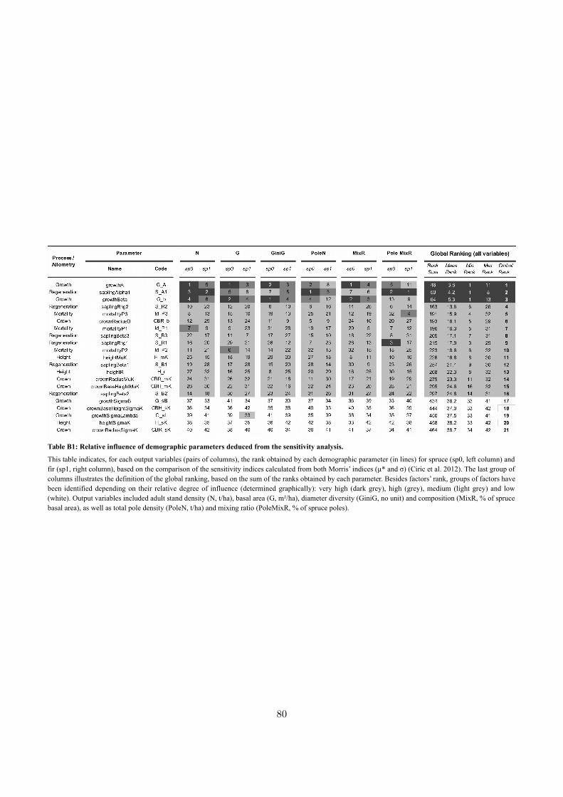
Table B1: Relative influence of demographic parameters deduced from the sensitivity analysis.
This table indicates, for each output variables (pairs of columns), the rank obtained by each demographic parameter (in lines) for spruce (sp0, left column) and
fir (sp1, right column), based on the comparison of the sensitivity indices calculated from both Morris’ indices (µ* and σ) (Ciric et al. 2012). The last group of
columns illustrates the definition of the global ranking, based on the sum of the ranks obtained by each parameter. Besides factors’ rank, groups of factors have
been identified depending on their relative degree of influence (determined graphically): very high (dark grey), high (grey), medium (light grey) and low
(white). Output variables included adult stand density (N, t/ha), basal area (G, m²/ha), diameter diversity (GiniG, no unit) and composition (MixR, % of spruce
basal area), as well as total pole density (PoleN, t/ha) and mixing ratio (PoleMixR, % of spruce poles).
80

Appendix C: Computation of relative errors
We took the posterior distributions obtained with 100,000 simulations as reference, and computed
relative errors on the mode and the 95% credible interval width (CIW) of the posterior distribution for
various simulation numbers i as:
Relative error modei=|Modei−Mode100000
Mode100 000
|
Relative errorCIW i=|CIW i−CIW100 000
CIW100000
|where Modei and CIWi are respectively the mode and the CIW computed on the posterior distributions
obtained with i simulations. We considered that relative errors smaller than 20% were acceptable, and
used this threshold value to estimate the number of required simulations to reach convergence in the
ABC recalibration procedure.
81
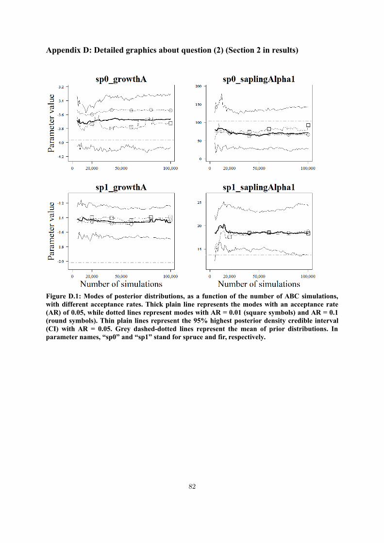
Appendix D: Detailed graphics about question (2) (Section 2 in results)
Figure D.1: Modes of posterior distributions, as a function of the number of ABC simulations,
with different acceptance rates. Thick plain line represents the modes with an acceptance rate
(AR) of 0.05, while dotted lines represent modes with AR = 0.01 (square symbols) and AR = 0.1
(round symbols). Thin plain lines represent the 95% highest posterior density credible interval
(CI) with AR = 0.05. Grey dashed-dotted lines represent the mean of prior distributions. In
parameter names, “sp0” and “sp1” stand for spruce and fir, respectively.
82
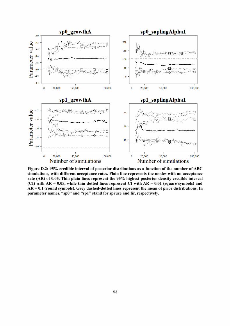
Figure D.2: 95% credible interval of posterior distributions as a function of the number of ABC
simulations, with different acceptance rates. Plain line represents the modes with an acceptance
rate (AR) of 0.05. Thin plain lines represent the 95% highest posterior density credible interval
(CI) with AR = 0.05, while thin dotted lines represent CI with AR = 0.01 (square symbols) and
AR = 0.1 (round symbols). Grey dashed-dotted lines represent the mean of prior distributions. In
parameter names, “sp0” and “sp1” stand for spruce and fir, respectively.
83
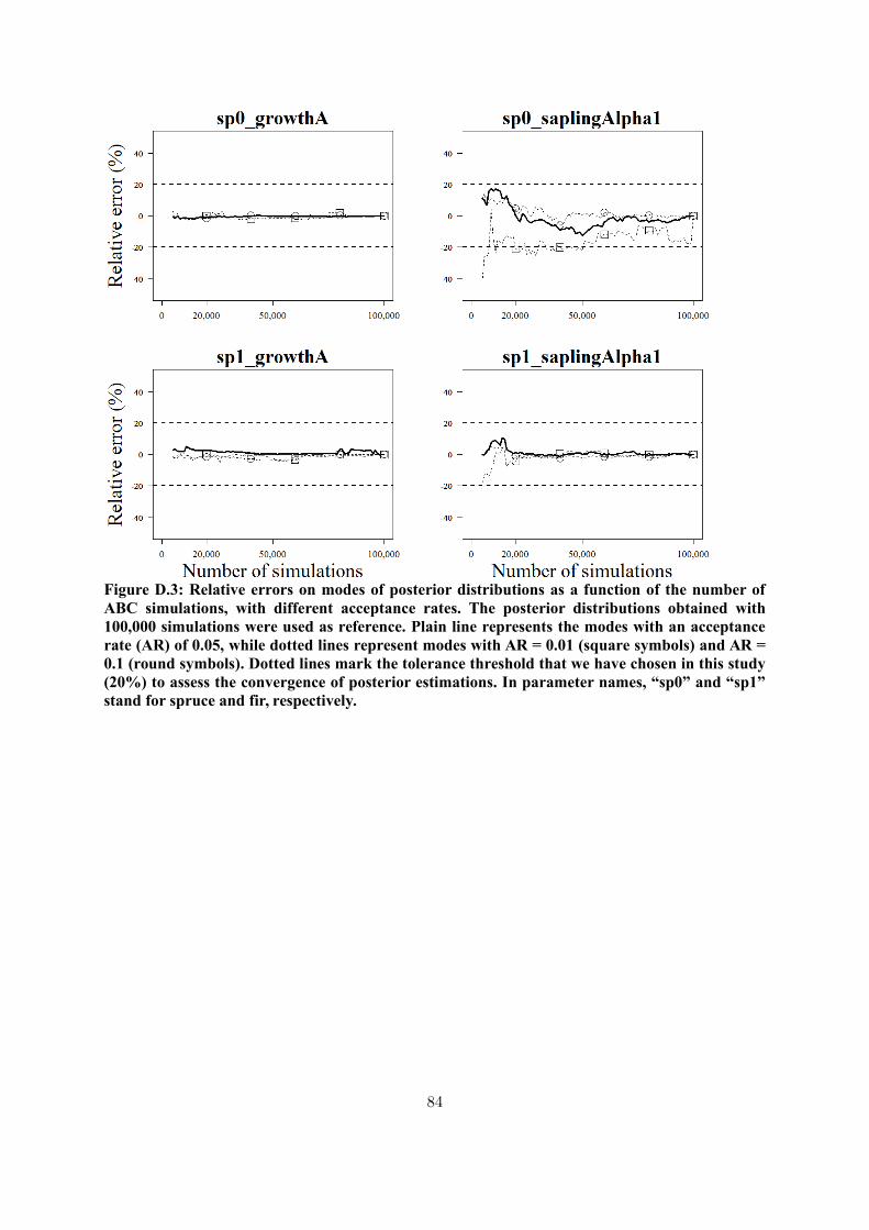
Figure D.3: Relative errors on modes of posterior distributions as a function of the number of
ABC simulations, with different acceptance rates. The posterior distributions obtained with
100,000 simulations were used as reference. Plain line represents the modes with an acceptance
rate (AR) of 0.05, while dotted lines represent modes with AR = 0.01 (square symbols) and AR =
0.1 (round symbols). Dotted lines mark the tolerance threshold that we have chosen in this study
(20%) to assess the convergence of posterior estimations. In parameter names, “sp0” and “sp1”
stand for spruce and fir, respectively.
84
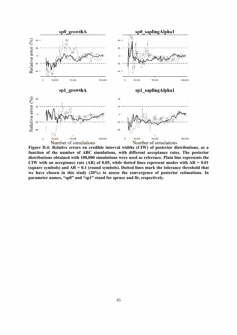
Figure D.4: Relative errors on credible interval widths (CIW) of posterior distributions, as a
function of the number of ABC simulations, with different acceptance rates. The posterior
distributions obtained with 100,000 simulations were used as reference. Plain line represents the
CIW with an acceptance rate (AR) of 0.05, while dotted lines represent modes with AR = 0.01
(square symbols) and AR = 0.1 (round symbols). Dotted lines mark the tolerance threshold that
we have chosen in this study (20%) to assess the convergence of posterior estimations. In
parameter names, “sp0” and “sp1” stand for spruce and fir, respectively.
85

Appendix E: R scripts used to explore the different questions
1. Create the designs of experiments (Sections 6.1, 6.2 and 6.3)
rm(list=ls())library(lhs) # for latin hypercubeslibrary(gdata) # to remove variables in data frames using their names
################################################ Script parameters #################################################################
Site <- "Prenovel"compartment <- 24 # Stand identifierinitialDate <- 1953finalDate <- 2011
folderIdOut <- "1c" # Local output folder identifierNSD_Out <- 1000 # Number of simulations to dolhsPartSize <- 1000 # Unitary size of the latin hypercube
# OptionsaugmentExistingLHS <- F # augment an pre-defined latin hypercube ?loadDOE <- T # Is the DOE sampled in posterior distributions ?folderIdIn <- "1b" # Local input folder identifier (used on ly if loadDOE is TRUE)useEstimator <- T # Do we use an estimator to summarize posterior distributions ? Else, sample directly in posterior distributions. (Used only if loadDOE is TRUE)estimator <- "median" # Posterior estimator (used only if useEstimator is TRUE)NSD_In <- 20000 # Number of simulations to doAR <- 0.01 # Number of simulations accepeted to compute posterior distributionsotherParFixed <- F # Est-ce que les paramètres non calibrés ont des valeurs fixes (plutôt que tirés dansune loi normale) ?
# Species names (in french)speciesNamesFR <- c("Epicea","Sapin")
# Model parameters to recalibrateparNames0 <- c() # M0parNames0 <- c("growthA") # M1parNames0 <- c("growthA","saplingAlpha1") # M2parNames0 <- c("growthA","saplingAlpha1","mortalityP1") # M3parNames0 <- c("growthA","saplingAlpha1","mortalityP1","growthBeta") # M4
# Set compartment text variablesfolderOutName <- paste0("C:/Users/guillaume.lagarrigue/Documents/IRSTEA/Thèse/Simulations/Simus S",folderIdOut,"/")folderObs <- paste0("C:/Users/guillaume.lagarrigue/Documents/IRSTEA/Données_Forêts/Données_",Site,"/Données_Traitées/")parNames <- paste0("sp",rep(0:(length(speciesNamesFR)-1),each=length(parNames0)),"_",parNames0) 86
################################################ Upload files ######################################################################
##### Upload parameter values, as computed in initial calibrationtab_par <- read.table(paste0(folderObs,"ParamUncertainty.csv"),h=T,sep=";",as.is=T)#### Data formattinginventoryFileNames <- paste0(Site,"_P",compartment,"_",initialDate,".inv")rownames(tab_par) <- tab_par$Param_sptab_par <- tab_par[,c("Param_sp","Mean","SD")]inputVarNames <- as.vector(tab_par$Param_sp)
########################################################################## Prior distributions ###################################################################################################################
# Initialize prior distribution tableinputLim <- as.data.frame(matrix(rep(0,length(inputVarNames)*2),ncol=2))rownames(inputLim) <- inputVarNamescolnames(inputLim) <- c("Min","Max")
# Set prior rangesinputLim[parNames,"Min"] <- tab_par[parNames,"Mean"] - 5*tab_par[parNames,"SD"]inputLim[parNames,"Max"] <- tab_par[parNames,"Mean"] + 5*tab_par[parNames,"SD"]inputLim[c("sp0_saplingAlpha1","sp1_saplingAlpha1"),"Min"] <- 0 # Computing bug in the model if <0
# Subset of prior table with only varying parameterstabSimu <- inputLim[which(inputLim$Min+inputLim$Max!=0),]
########################################################################## DOE ###################################################################################################################################
### DOE creationif (!loadDOE) { # Create a new DOE if (nrow(tabSimu) != 0) { # At least one parameter is varying if (!augmentExistingLHS) { # Create a new latin hypercube samplingTab <- randomLHS(lhsPartSize,nrow(tabSimu)) # First iteration to create the latin hypercube lhsIterations <- NSD_Out / lhsPartSize # Number of iterations to create the whole DOE
# Augment the first LH until reaching the desired size (= NSD_Out) if (lhsIterations > 1){ for (i in 2:lhsIterations) { print(paste0("LHS augmentation, iteration : ",i)) samplingTab <- augmentLHS(samplingTab,NSD_Out / lhsIterations) } } # Save the DOE write.table(x=samplingTab,file=paste0(folderOutName,"lhs.txt"),sep="\t",row.names=F,quote=F) } else { # Augment an pre-existing LH (used for the question: how many simulations to run ?)
87
samplingTab <- as.matrix(read.table(paste0(folderOutName,"lhs.txt"),h=T)) # Augment the first LH until reaching the desired size (= NSD_Out) while (nrow(samplingTab) < NSD_Out) { print(paste0("LHS augmentation, iteration : ",nrow(samplingTab) / (NSD_Out / lhsIterations)+1)) samplingTab <- augmentLHS(samplingTab,NSD_Out / lhsIterations) } # Save the DOE write.table(x=samplingTab,file=paste0(folderOutName,"lhs.txt"),sep="\t",row.names=F,quote=F) }
# Set DOE values : from [0,1] intervals to prior ranges computeLHSValues <- function(v) { return(as.numeric(sprintf("%.5f", (tabSimu$Min + v * (tabSimu$Max - tabSimu$Min))))) }
samplingTab <- t(apply(samplingTab,1,computeLHSValues)) samplingTab <- as.data.frame(samplingTab) colnames(samplingTab) <- rownames(tabSimu) } else { samplingTab <- data.frame() # To simulate only model stochasticity }
} else { # Create a DOE using posterior distributions (to check model outputs after recalibration) ## Upload posterior values selectedSimus <- read.table(paste0(paste0("C:/Users/guillaume.lagarrigue/Documents/IRSTEA/Thèse/Simulations/Simus S",folderIdIn,"/"),"selectedSimus_NSD",NSD_In,"_AR",AR,".txt"),h=T) if (length(unique(selectedSimus$Date))>1) selectedSimus <- subset(selectedSimus,Date==finalDate) selectedSimus$ParName <- paste0("sp",selectedSimus$Species,"_",selectedSimus$Parameter) if (useEstimator) { #### The DOE is a repetition of the same value # Function to estimate the first mode of a distribution (useful when the estimator is the mode) distMode <- function(v) { d <- density(v) return(d$x[which(d$y==max(d$y))][1]) }
# Summarize posterior distributions, using the selected estimator tab <- aggregate(data.frame(Value=selectedSimus$Value),by=list(ParName=selectedSimus$ParName),FUN=estimator) rownames(tab) <- tab$ParName tab <- remove.vars(tab,"ParName") samplingTab <- as.data.frame(matrix(rep(tab[parNames,"Value"],each=NSD_Out),ncol=length(parNames))) colnames(samplingTab) <- parNames } else { #### The DOE is randomly sampled in the posterior distributions tabIn <- unstack(selectedSimus,Value~ParName) samplingTab <- tabIn[sample(nrow(tabIn),NSD_Out,replace=TRUE),parNames] }}
88

########################################################################## Generate the input table to run simulations with Capsis ###############################################################################
# Create a table where all parameters are randomly sampled normal distributions based on initial calibrationfor (i in 1:nrow(tab_par)) { v <- rnorm(NSD_Out,tab_par$Mean[i],tab_par$SD[i]) if (i==1) { normTab <- v } else { normTab <- cbind(normTab,v) }}colnames(normTab) <- tab_par$Param_sp
# Initialize the output tabletabFinal <- as.data.frame(matrix(rep(0,NSD_Out*length(compartment)*(3+length(inputVarNames))),ncol=length(inputVarNames)+3))colnames(tabFinal) <- c("InventoryFileName","Forest","Compartment",inputVarNames)
# Initially, the output table is filled using mean values from intial calibration for all parameterstabFinal[,4:(nrow(tab_par)+3)] <- as.data.frame(matrix(rep(tab_par$Mean,NSD_Out*length(compartment)),ncol=nrow(tab_par),byrow=T))
# Replace fixed values by random values for non recalibrated parameters (option)if (!otherParFixed) { tabFinal[,colnames(normTab)] <- normTab}
# Replace fixed values by values from DOE for recalibrated parameterstabFinal[,colnames(samplingTab)] <- samplingTab
# Other settingstabFinal$InventoryFileName <- inventoryFileNamestabFinal$Forest <- SitetabFinal$Compartment <- compartment
########## Save files ###### Table used for posterior analyzeswrite.table(x=tabFinal,file=paste0(folderOutName,"inputTab.txt"),sep="\t",row.names=F,quote=F)
# Table used to run simulations in Capsis (the same without titles)write.table(x=tabFinal,file=paste0(folderOutName,"commandFile.csv"),sep="\t",row.names=F,col.names=F,quote=F)
2. Get the posterior distributions (Section 6.1)
rm(list=ls())library(abc) # to estimate parameter values with ABC
89

################################################ Script parameters #################################################################
Site <- "Prenovel"compartment <- 24 # Identifiants peuplementsdate <- 2011
# Diameter classesfirstClass <- 20lastClass <- c(65,65)classWidth <- 5
# Species names (in french)speciesNamesFR <- c("Epicea","Sapin")
speciesAcronyms <- c("PIAB","ABAL")
folderIdIn <- "1b"NSD <- 20000 # Number of Simulations DoneAR <- 0.01 # Acceptance rateparNames0 <-c("growthA")parNames0 <- c("growthA","saplingAlpha1")parNames0 <- c("growthA","saplingAlpha1","mortalityP1")parNames0 <- c("growthA","saplingAlpha1","mortalityP1","growthBeta")
################################################ Script variable definition ########################################################
# Folder pathesfolderInName <- paste0("C:/Users/guillaume.lagarrigue/Documents/IRSTEA/Thèse/Simulations/Simus S",folderIdIn,"/")folderObs <- paste0("C:/Users/guillaume.lagarrigue/Documents/IRSTEA/Données_Forêts/Données_",Site,"/Données_Traitées/")
# Parameter namesparNames <- paste0("sp",rep(0:(length(speciesNamesFR)-1),each=length(parNames0)),"_",parNames0)
# Diameter classes, by speciesDclassesNamesSp <- c()for(sp in 1:length(speciesNamesFR)) { DclassesNamesSp <- c(DclassesNamesSp,paste0("sp",sp-1,c(paste0("_D",seq(firstClass,lastClass[sp],classWidth)),"_G_LT")))}
# Summary statistics namesssNamesDC <- paste0(DclassesNamesSp)ssNames <- c(ssNamesDC,"CutV.Cum")
90
################################################ Upload files ######################################################################
# Observed stand valuesinv <- read.table(file=paste0(folderObs,"inventoriesWithStandVariables.txt"),header=T,as.is=T)
# DOEinput <- read.table(paste0(folderInName,"inputTab.txt"),h=T)
# Simulation resultsoutput <- read.table(paste0(folderInName,"Histo_P",compartment,"_",date,".txt"),h=T)
# Data formattinginvR <- subset(inv,Compartment==compartment & Year==date)dc <- c(paste0("D",seq(firstClass,125,5)),"G_LT")dcsp <- paste0(rep(paste0("sp",0:1),each=length(dc)),"_",rep(dc,2))stats <- as.data.frame(matrix(unlist(as.vector(t(as.matrix(invR[which(invR$Species %in% speciesAcronyms),dc])))),nrow=1,dimnames=list(1,dcsp)))
########################################################## Compute target and simulated harvestings #################### over the whole time period ########################################################################
# Upload dataoutput2 <- read.table(paste0(folderInName,"output2_P",compartment,".txt"),h=T)
# Data formattingoutput2 <- subset(output2,SpType==1) # Sélection des coupes sur les résineux seulementinterventionDates <- unique(output2$InterventionId)output2 <- output2[1:(NSD*length(interventionDates)),] output2$SimulationId <- rep(1:NSD,each=length(interventionDates))output2$Date <- interventionDatescutV <- aggregate(output2[,c("TargetV","CutV")],by=list(SimulationId=output2$SimulationId),FUN=sum)
# Target harvesting -> observed datastats <- cbind(stats,CutV.Cum=unique(cutV$TargetV))
# Simulated harvesting -> simulated dataoutput <- cbind(output,CutV.Cum=cutV$CutV)
################################################ Compute posterior distributions ###################################################
# Set abc() function parameterstarget <- as.vector(as.matrix(stats[,ssNames]))sumstat <- output[,ssNames]param <- input[,parNames]tol <- ARmethod <- "loclinear" # Local linear regressions (Beaumont et al., 2002)
# Apply ABC function and get accepted values91

ABC <- abc(target,param,sumstat,tol,method)df <- ABC$adj.values
################################################ Create and save output table ######################################################selectedSimus <- data.frame(NSA=NSD*AR ,Plot=compartment ,Date=date ,Parameter=rep(parNames0,each=NSD*AR) ,Species=rep(0:(length(speciesNamesFR)-1),each=length(parNames0)*NSD*AR) ,Value=as.vector(as.matrix(df[,1:length(parNames)])))
write.table(selectedSimus,paste0(folderInName,"selectedSimus_NSD",NSD,"_AR",AR,".txt"),sep="\t",row.names=F)
3. Process model selection using Bayes factor (Section 6.1)
rm(list=ls())library(abc) # For postpr() and cv4postpr() functions
################################################ Script parameters #################################################################
Site <- "Prenovel"compartment <- 24 # Identifiants peuplementsdate <- 2011
# Diameter classesfirstClass <- 20lastClass <- c(65,65)classWidth <- 5
# Species names (in french)speciesNamesFR <- c("Epicea","Sapin")
speciesAcronyms <- c("PIAB","ABAL")
NSD <- 20000 # Number of Simulations DoneAR <- 0.01 # Acceptance rate
################################################ Script variable definition ########################################################
# Folder pathesfolderObs <- paste0("C:/Users/guillaume.lagarrigue/Documents/IRSTEA/Données_Forêts/Données_",Site,"/Données_Traitées/")
# Diameter classes, by speciesDclassesNamesSp <- c()
92
for(sp in 1:length(speciesNamesFR)) { DclassesNamesSp <- c(DclassesNamesSp,paste0("sp",sp-1,c(paste0("_D",seq(firstClass,lastClass[sp],classWidth)),"_G_LT")))}
# Summary statistics namesssNamesDC <- paste0(DclassesNamesSp)ssNames <- c(ssNamesDC,"CutV.Cum")
################################################ Upload files ######################################################################
# Observed stand valuesinv <- read.table(file=paste0(folderObs,"inventoriesWithStandVariables.txt"),header=T,as.is=T)
# Data formattinginvR <- subset(inv,Compartment==compartment & Year==date)dc <- c(paste0("D",seq(firstClass,125,5)),"G_LT")dcsp <- paste0(rep(paste0("sp",0:1),each=length(dc)),"_",rep(dc,2))stats <- as.data.frame(matrix(unlist(as.vector(t(as.matrix(invR[which(invR$Species %in% speciesAcronyms),dc])))),nrow=1,dimnames=list(1,dcsp)))
################################################### Model selection #############################################################
withM0 <- FALSE
if(withM0) { folderIdIn <- 1:5 parNames0 <- list( c() ,c("growthA") ,c("growthA","saplingAlpha1") ,c("growthA","saplingAlpha1","mortalityP1") ,c("growthA","saplingAlpha1","mortalityP1","growthBeta") ) index <- rep(0:4,each=NSD)} else { folderIdIn <- 2:5 parNames0 <- list( c("growthA") ,c("growthA","saplingAlpha1") ,c("growthA","saplingAlpha1","mortalityP1") ,c("growthA","saplingAlpha1","mortalityP1","growthBeta") ) index <- rep(1:4,each=NSD)}# Upload simulation outputsoutputList <- list()
for (iModele in 1:length(folderIdIn)) { # Iteration over all models
# Set the parameter names for this model93

parNames <- paste0("sp",rep(0:(length(speciesNamesFR)-1),each=length(parNames0[[iModele]])),"_",parNames0[[iModele]]) folderPath <- paste0("C:/Users/guillaume.lagarrigue/Documents/IRSTEA/Thèse/Simulations/Simus S",folderIdIn[iModele],"/") output <- read.table(paste0(folderPath,"Histo_P",compartment,"_",date,".txt"),h=T)
### Compute target and simulated harvestings over the whole time period ################# # Upload data output2 <- read.table(paste0(folderPath,"output2_P",compartment,".txt"),h=T) # Data formatting output2 <- subset(output2,SpType==1) # Sélection des coupes sur les résineux seulement interventionDates <- unique(output2$InterventionId) output2 <- output2[1:(nrow(output)*length(interventionDates)),] output2$SimulationId <- rep(1:nrow(output),each=length(interventionDates)) output2$Date <- interventionDates cutV <- aggregate(output2[,c("TargetV","CutV")],by=list(SimulationId=output2$SimulationId),FUN=sum) # Target harvesting -> observed data stats <- cbind(stats,CutV.Cum=unique(cutV$TargetV)) # Simulated harvesting -> simulated data output <- cbind(output,CutV.Cum=cutV$CutV) # Save output table in a list outputList[[iModele]] <- output[1:NSD,]}
# Set postpr() function parameterstarget <- stats[,ssNames]sumstat <- outputList[[1]][,ssNames]for (iModele in 2:length(folderIdIn)) { sumstat <- rbind(sumstat,outputList[[iModele]][,ssNames])}tol <- ARmethod <- "mnlogistic" # Multinomial logistic regressions (Beaumont, 2008)
# Compute Bayes factorPP <- postpr(target=target,index=index,sumstat=sumstat,tol=tol,method=method)summary(PP)
# Process cross validationsCVPP <- cv4postpr(index,sumstat,PP,100,tol,method=method)summary(CVPP)
4. Check ABC convergence (Section 6.2)
rm(list=ls())library(abc)library(LaplacesDemon) # To compute credible intervals
################################################ Script parameters #####################
94

############################################
Site <- "Prenovel"compartment <- 24 # Stand identifierdate <- 2011
# Diameter classesfirstClass <- 20lastClass <- c(65,65)classWidth <- 5
# Species names (in french)speciesNamesFR <- c("Epicea","Sapin")
speciesAcronyms <- c("PIAB","ABAL")
folderIdIn <- 74NSDv <- seq(1000,10000,1000) # Number of Simulations DoneARv <- c(0.005,0.01,0.02,0.05,0.1) # Acceptance rateparNames0 <- c("growthA","saplingAlpha1")
################################################ Script variable definition ########################################################
# Folder pathesfolderInName <- paste0("C:/Users/guillaume.lagarrigue/Documents/IRSTEA/Thèse/Simulations/Simus S",folderIdIn,"/")folderObs <- paste0("C:/Users/guillaume.lagarrigue/Documents/IRSTEA/Données_Forêts/Données_",Site,"/Données_Traitées/")
# Parameter namesparNames <- paste0("sp",rep(0:(length(speciesNamesFR)-1),each=length(parNames0)),"_",parNames0)
# Diameter classes, by speciesDclassesNamesSp <- c()for(sp in 1:length(speciesNamesFR)) { DclassesNamesSp <- c(DclassesNamesSp,paste0("sp",sp-1,c(paste0("_D",seq(firstClass,lastClass[sp],classWidth)),"_G_LT")))}
# Summary statistics namesssNamesDC <- paste0(DclassesNamesSp)ssNames <- c(ssNamesDC,"CutV.Cum")
# Function to estimate the first mode of a distribution (useful when the estimator is the mode)distMode <- function(v) { d <- density(v) return(d$x[which(d$y==max(d$y))][1])}
############################################95
#### Upload files ######################################################################
# Observed stand valuesinv <- read.table(file=paste0(folderObs,"inventoriesWithStandVariables.txt"),header=T,as.is=T)
# DOEinput <- read.table(paste0(folderInName,"inputTab.txt"),h=T)
# Simulation resultsoutput <- read.table(paste0(folderInName,"Histo_P",compartment,"_",date,".txt"),h=T)
# Data formattinginvR <- subset(inv,Compartment==compartment & Year==date)dc <- c(paste0("D",seq(firstClass,125,5)),"G_LT")dcsp <- paste0(rep(paste0("sp",0:1),each=length(dc)),"_",rep(dc,2))stats <- as.data.frame(matrix(unlist(as.vector(t(as.matrix(invR[which(invR$Species %in% speciesAcronyms),dc])))),nrow=1,dimnames=list(1,dcsp)))
################################################ Initialize output table ######################################################outputTab <- data.frame(NSD=0,AR=0,ParName=0,Mode=0,Median=0,Mean=0,SD=0,CI_sup=0,CI_inf=0)
########################################################## Compute target and simulated harvestings #################### over the whole time period ########################################################################
# Upload dataoutput2 <- read.table(paste0(folderInName,"output2_P",compartment,".txt"),h=T)
# Data formattingoutput2 <- subset(output2,SpType==1) # Sélection des coupes sur les résineux seulementinterventionDates <- unique(output2$InterventionId)output2 <- output2[1:(max(NSDv)*length(interventionDates)),] output2$SimulationId <- rep(1:max(NSDv),each=length(interventionDates))output2$Date <- interventionDatescutV <- aggregate(output2[,c("TargetV","CutV")],by=list(SimulationId=output2$SimulationId),FUN=sum)
# Target harvesting -> observed datastats <- cbind(stats,CutV.Cum=unique(cutV$TargetV))
# Simulated harvesting -> simulated dataoutput <- cbind(output,CutV.Cum=cutV$CutV)
################################################ Iterate on NSD and AR values ###################################################
for (iNSD in 1:length(NSDv)) {96
NSD <- NSDv[iNSD] print(paste0("Processing NSD = ",NSD)) inputR <- input[1:NSD,] outputR <- output[1:NSD,] for (iAR in 1:length(ARv)) { AR <- ARv[iAR] print(paste0("Processing AR = ",AR))
############################################ #### Compute posterior distributions ####### ############################################ # Set abc() function parameters target <- as.vector(as.matrix(stats[,ssNames])) sumstat <- output[,ssNames] param <- input[,parNames] tol <- AR method <- "loclinear" # Local linear regressions (Beaumont et al., 2002) # Apply ABC function and get accepted values ABC <- abc(target,param,sumstat,tol,method) df <- ABC$adj.values
################################### #### Update output table ########## ################################### for (iPN in 1:length(parNames)) { parName <- parNames[iPN] outputTab <- rbind(outputTab,data.frame(NSD=NSD ,AR=AR ,ParName=parName ,Mode=distMode(df[,parName]) ,Median=median(df[,parName]) ,Mean=mean(df[,parName]) ,SD=sd(df[,parName]) ,CI_sup=as.numeric(p.interval(df[,parName],MM=F)[,"Upper"]) ,CI_inf=as.numeric(p.interval(df[,parName],MM=F)[,"Lower"]) )) } }}
##################################### Save output table ###########################################
outputTab <- outputTab[-1,]write.table(outputTab,paste0(folderInName,"ABC_Convergence.txt"),sep="\t",row.names=F)
5. Propagation of uncertainties (Section 6.3)
rm(list=ls())97
################################################ Script parameters #################################################################
Site <- "Prenovel"compartment <- 24 # Identifiants peuplementsdate <- 2011
# Diameter classesfirstClass <- 20lastClass <- c(65,65)classWidth <- 5
# Species names (in french)speciesNamesFR <- c("Epicea","Sapin")
speciesAcronyms <- c("PIAB","ABAL")
NSD <- 1000 # Number of Simulations Done
################################################ Script variable definition ########################################################
# Folder pathesfolderObs <- paste0("C:/Users/guillaume.lagarrigue/Documents/IRSTEA/Données_Forêts/Données_",Site,"/Données_Traitées/")
# Diameter classes, by speciesDclassesNamesSp <- c()for(sp in 1:length(speciesNamesFR)) { DclassesNamesSp <- c(DclassesNamesSp,paste0("sp",sp-1,c(paste0("_D",seq(firstClass,lastClass[sp],classWidth)),"_G_LT")))}
# Summary statistics namesssNamesDC <- paste0(DclassesNamesSp)ssNames <- c(ssNamesDC,"CutV.Cum")
################################################ Upload files ######################################################################
# Observed stand valuesinv <- read.table(file=paste0(folderObs,"inventoriesWithStandVariables.txt"),header=T,as.is=T)
# Data formattinginvR <- subset(inv,Compartment==compartment & Year==date)dc <- c(paste0("D",seq(firstClass,125,5)),"G_LT")dcsp <- paste0(rep(paste0("sp",0:1),each=length(dc)),"_",rep(dc,2))stats <- as.data.frame(matrix(unlist(as.vector(t(as.matrix(invR[which(invR$Species %in% speciesAcronyms),dc])))),nrow=1,dimnames=list(1,dcsp)))
98

############################################################################################### Compute mean and standard deviations on model outputs ###############################################################################################################
folderIdIn <- c(77:79)
for (i in 1:length(folderIdIn)) { folderPath <- paste0("C:/Users/guillaume.lagarrigue/Documents/IRSTEA/Thèse/Simulations/Simus S",folderIdIn[i],"/") output <- read.table(paste0(folderPath,"Histo_P",compartment,"_",date,".txt"),h=T)
### Compute target and simulated harvestings over the whole time period ################# # Upload data output2 <- read.table(paste0(folderPath,"output2_P",compartment,".txt"),h=T) # Data formatting output2 <- subset(output2,SpType==1) # Sélection des coupes sur les résineux seulement interventionDates <- unique(output2$InterventionId) output2 <- output2[1:(nrow(output)*length(interventionDates)),] output2$SimulationId <- rep(1:nrow(output),each=length(interventionDates)) output2$Date <- interventionDates cutV <- aggregate(output2[,c("TargetV","CutV")],by=list(SimulationId=output2$SimulationId),FUN=sum) # Target harvesting -> observed data stats <- cbind(stats,CutV.Cum=unique(cutV$TargetV)) # Simulated harvesting -> simulated data output <- cbind(output,CutV.Cum=cutV$CutV) if(i==1) { tabOut <- data.frame(SimuId=i ,Stat=ssNames ,Mean=round(apply(output[,ssNames],2,mean),2) ,SD=round(apply(output[,ssNames],2,sd),2) ) } else { tabOut <- rbind(tabOut,data.frame(SimuId=i ,Stat=ssNames ,Mean=round(apply(output[,ssNames],2,mean),2) ,SD=round(apply(output[,ssNames],2,sd),2) )) }}
SDs <- unstack(tabOut,SD~SimuId)
SDs$X13p <- SDs$X1 / SDs$X3 *100SDs$X23p <- SDs$X2 / SDs$X3 *100SDs["Mean",] <- apply(SDs,2,mean)
# Variability of model predictions due to model stochasticity99

SDs["Mean","X13p"]
# Variability of model predictions due to uncertainties on recalibrated parametersSDs["Mean","X23p"] - SDs["Mean","X13p"]
# Variability of model predictions due to uncertainties on non-recalibrated parameters100 - SDs["Mean","X23p"]
100

Bibliography
Beaumont, M.A. 2008 Joint determination of topology, divergence time, and immigration in
population trees. Renfrew C Matsumura S, Forster P, editor, Simulation, Genetics and Human
Prehistory, McDonald Institute Monographs, 134-1541.
Beaumont, M.A., Zhang, W.Y. and Balding, D.J. 2002 Approximate Bayesian computation in
population genetics. Genetics, 162, 2025-2035.
Campolongo, F., Cariboni, J. and Saltelli, A. 2007 An effective screening design for sensitivity
analysis of large models. Environmental Modelling & Software, 22, 1509-1518.
Ciric, C., Ciffroy, P. and Charles, S. 2012 Use of sensitivity analysis to identify influential and non-
influential parameters within an aquatic ecosystem model. Ecological Modelling, 246, 119-130.
Courbaud, B., de Coligny, F. and Cordonnier, T. 2003 Simulating radiation distribution in a
heterogeneous Norway spruce forest on a slope. Agricultural and Forest Meteorology, 116, 1-18.
Goreaud, F., Loussier, B., M.A., N.B. and R., A. 2004 Simulating realistic spatial structure for forest
stands : a mimetic point process. p. 22p.
Morris, M.D. 1991 Factorial Sampling Plans for Preliminary Computational Experiments.
Technometrics, 33, 161-174.
Pujol, G., Iooss, B. and Janon, A. 2012 sensitivity: Sensitivity Analysis. R package version 1.6-1.
http://CRAN.R-project.org/package=sensitivity.
R Development Core Team. 2011 R : A language and environment for statistical computing. R
Foundation for Statistical Computing, Vienna, Austria.
Ripley, B.D. 1977 Modelling spatial patterns. Journal of the Royal Statistical Society. Series B
(Methodological), 172-212.
Vieilledent, G., Courbaud, B., Kunstler, G., Dhote, J.F. and Clark, J.S. 2010 Individual variability in
tree allometry determines light resource allocation in forest ecosystems: a hierarchical Bayesian
approach. Oecologia, 163, 759-773.
101

Annexe B : article asscoié à la partie 3
Article en préparation pour European Journal of Forest Research
102
Demographic variability in spruce-ir-beech forest stands in Europe
Guillaume Lagarrigues1*, Franck Jabot2, Andreas Zingg3, Jean-Claude Gégout4,5, MatijaKlopčič6, Benoît Courbaud1
1. Université Grenoble Alpes, Irstea, UR EMGR, 2 rue de la Papeterie-BP 76, F-38402 St-Martin-d’Hères, France.
2. LISC-Laboratoire d’Ingénierie pour les Systèmes complexes, IRSTEA, 9 Avenue Blaise Pascal,CS 20085, 63178 Aubière, France
3. Forest Resources and Management, Swiss Federal Research Institute WSL, Zürcherstrasse 111,CH-8903 Birmensdorf, Switzerland
4. AgroParisTech, UMR 1092, Laboratoire d’Etude des ressources Forêt-Bois (LERFoB), 54042Nancy, France
5. INRA, UMR 1092,Laboratoire d’Etude des ressources Forêt-Bois (LERFoB), 54280 Champenoux,France
6. Department of Forestry and Renewable Forest Resources, Biotechnical Faculty, University ofLjubljana, Vecna Pot 83, 1000, Ljubljana, Slovenia
*Corresponding author : Guillaume Lagarrigues
Email : [email protected]
Phone number : +33 (0)4 76 76 27 07
Fax number : +33 (0)4 76 51 38 03
103

1 Abstract
Many studies have predicted large changes in forest dynamics during the next century because of globalwarming. Although empirical approaches and studies based on species distribution models providevaluable information about future changes, they do not take into account biotic interactions andstand-level demographic variations. The objective of this study was to quantify the local and regionalvariability of the growth and regeneration of three important forest species growing often in mixedstands in Europe (Picea abies (L.) Karst., Abies alba Mill., Fagus sylvatica), and to assess the climaticdrivers of this variability. For that purpose, we collected a large forestry data set compiling the long-term (up to 100 years) evolution of species and size distributions for 163 stands across Europe, in themesic distribution area of these forests. We used an inverse modeling approach, Approximate BayesianComputation, to calibrate an individual-based model of forest dynamics on these data. Our studyrevealed that the variability of the demographic processes was of the same order of magnitude betweenstands of a same forest as between diferent forests. Out of the three species and two demographicprocesses studied, only the ir growth strongly varied with temperature. Water availability did notexplain any demographic variation over stands. For these forests experiencing mesic conditions, localunmeasured factors seem therefore to have an inluence at least as important as macro-environmentalfactors on demographic variations. Eforts to include these important factors in projection scenariosshould therefore be prioritized. Besides, our study demonstrates that inverse modelling methods makepossible the analysis of long-term forestry data. Such data should therefore be more widely compiledand used for ecological and global change research.
104

2 Key-words
• Approximate Bayesian Computation• Climate change• Dynamic vegetation models• Forest ecology• Plant population and community dynamics• Samsara2
105
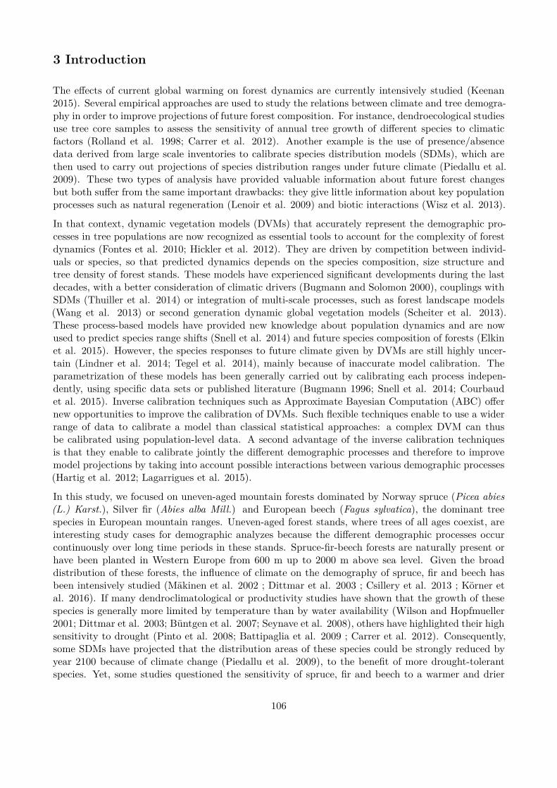
3 Introduction
The efects of current global warming on forest dynamics are currently intensively studied (Keenan2015). Several empirical approaches are used to study the relations between climate and tree demogra-phy in order to improve projections of future forest composition. For instance, dendroecological studiesuse tree core samples to assess the sensitivity of annual tree growth of diferent species to climaticfactors (Rolland et al. 1998; Carrer et al. 2012). Another example is the use of presence/absencedata derived from large scale inventories to calibrate species distribution models (SDMs), which arethen used to carry out projections of species distribution ranges under future climate (Piedallu et al.2009). These two types of analysis have provided valuable information about future forest changesbut both sufer from the same important drawbacks: they give little information about key populationprocesses such as natural regeneration (Lenoir et al. 2009) and biotic interactions (Wisz et al. 2013).
In that context, dynamic vegetation models (DVMs) that accurately represent the demographic pro-cesses in tree populations are now recognized as essential tools to account for the complexity of forestdynamics (Fontes et al. 2010; Hickler et al. 2012). They are driven by competition between individ-uals or species, so that predicted dynamics depends on the species composition, size structure andtree density of forest stands. These models have experienced signiicant developments during the lastdecades, with a better consideration of climatic drivers (Bugmann and Solomon 2000), couplings withSDMs (Thuiller et al. 2014) or integration of multi-scale processes, such as forest landscape models(Wang et al. 2013) or second generation dynamic global vegetation models (Scheiter et al. 2013).These process-based models have provided new knowledge about population dynamics and are nowused to predict species range shifts (Snell et al. 2014) and future species composition of forests (Elkinet al. 2015). However, the species responses to future climate given by DVMs are still highly uncer-tain (Lindner et al. 2014; Tegel et al. 2014), mainly because of inaccurate model calibration. Theparametrization of these models has been generally carried out by calibrating each process indepen-dently, using speciic data sets or published literature (Bugmann 1996; Snell et al. 2014; Courbaudet al. 2015). Inverse calibration techniques such as Approximate Bayesian Computation (ABC) ofernew opportunities to improve the calibration of DVMs. Such lexible techniques enable to use a widerrange of data to calibrate a model than classical statistical approaches: a complex DVM can thusbe calibrated using population-level data. A second advantage of the inverse calibration techniquesis that they enable to calibrate jointly the diferent demographic processes and therefore to improvemodel projections by taking into account possible interactions between various demographic processes(Hartig et al. 2012; Lagarrigues et al. 2015).
In this study, we focused on uneven-aged mountain forests dominated by Norway spruce (Picea abies(L.) Karst.), Silver ir (Abies alba Mill.) and European beech (Fagus sylvatica), the dominant treespecies in European mountain ranges. Uneven-aged forest stands, where trees of all ages coexist, areinteresting study cases for demographic analyzes because the diferent demographic processes occurcontinuously over long time periods in these stands. Spruce-ir-beech forests are naturally present orhave been planted in Western Europe from 600 m up to 2000 m above sea level. Given the broaddistribution of these forests, the inluence of climate on the demography of spruce, ir and beech hasbeen intensively studied (Mäkinen et al. 2002 ; Dittmar et al. 2003 ; Csillery et al. 2013 ; Körner etal. 2016). If many dendroclimatological or productivity studies have shown that the growth of thesespecies is generally more limited by temperature than by water availability (Wilson and Hopfmueller2001; Dittmar et al. 2003; Büntgen et al. 2007; Seynave et al. 2008), others have highlighted their highsensitivity to drought (Pinto et al. 2008; Battipaglia et al. 2009 ; Carrer et al. 2012). Consequently,some SDMs have projected that the distribution areas of these species could be strongly reduced byyear 2100 because of climate change (Piedallu et al. 2009), to the beneit of more drought-tolerantspecies. Yet, some studies questioned the sensitivity of spruce, ir and beech to a warmer and drier
106
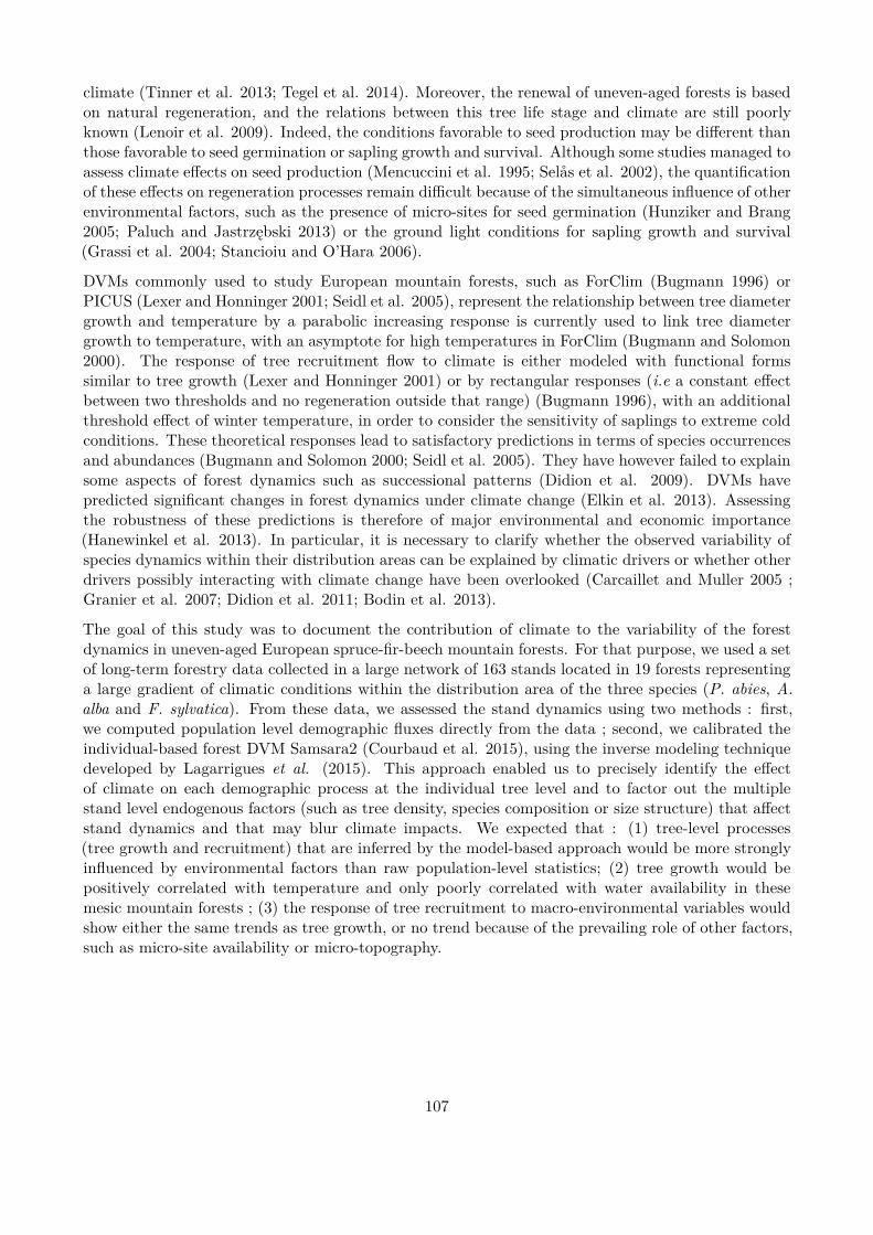
climate (Tinner et al. 2013; Tegel et al. 2014). Moreover, the renewal of uneven-aged forests is basedon natural regeneration, and the relations between this tree life stage and climate are still poorlyknown (Lenoir et al. 2009). Indeed, the conditions favorable to seed production may be diferent thanthose favorable to seed germination or sapling growth and survival. Although some studies managed toassess climate efects on seed production (Mencuccini et al. 1995; Selås et al. 2002), the quantiicationof these efects on regeneration processes remain diicult because of the simultaneous inluence of otherenvironmental factors, such as the presence of micro-sites for seed germination (Hunziker and Brang2005; Paluch and Jastrzębski 2013) or the ground light conditions for sapling growth and survival(Grassi et al. 2004; Stancioiu and O’Hara 2006).
DVMs commonly used to study European mountain forests, such as ForClim (Bugmann 1996) orPICUS (Lexer and Honninger 2001; Seidl et al. 2005), represent the relationship between tree diametergrowth and temperature by a parabolic increasing response is currently used to link tree diametergrowth to temperature, with an asymptote for high temperatures in ForClim (Bugmann and Solomon2000). The response of tree recruitment low to climate is either modeled with functional formssimilar to tree growth (Lexer and Honninger 2001) or by rectangular responses (i.e a constant efectbetween two thresholds and no regeneration outside that range) (Bugmann 1996), with an additionalthreshold efect of winter temperature, in order to consider the sensitivity of saplings to extreme coldconditions. These theoretical responses lead to satisfactory predictions in terms of species occurrencesand abundances (Bugmann and Solomon 2000; Seidl et al. 2005). They have however failed to explainsome aspects of forest dynamics such as successional patterns (Didion et al. 2009). DVMs havepredicted signiicant changes in forest dynamics under climate change (Elkin et al. 2013). Assessingthe robustness of these predictions is therefore of major environmental and economic importance(Hanewinkel et al. 2013). In particular, it is necessary to clarify whether the observed variability ofspecies dynamics within their distribution areas can be explained by climatic drivers or whether otherdrivers possibly interacting with climate change have been overlooked (Carcaillet and Muller 2005 ;Granier et al. 2007; Didion et al. 2011; Bodin et al. 2013).
The goal of this study was to document the contribution of climate to the variability of the forestdynamics in uneven-aged European spruce-ir-beech mountain forests. For that purpose, we used a setof long-term forestry data collected in a large network of 163 stands located in 19 forests representinga large gradient of climatic conditions within the distribution area of the three species (P. abies, A.alba and F. sylvatica). From these data, we assessed the stand dynamics using two methods : irst,we computed population level demographic luxes directly from the data ; second, we calibrated theindividual-based forest DVM Samsara2 (Courbaud et al. 2015), using the inverse modeling techniquedeveloped by Lagarrigues et al. (2015). This approach enabled us to precisely identify the efectof climate on each demographic process at the individual tree level and to factor out the multiplestand level endogenous factors (such as tree density, species composition or size structure) that afectstand dynamics and that may blur climate impacts. We expected that : (1) tree-level processes(tree growth and recruitment) that are inferred by the model-based approach would be more stronglyinluenced by environmental factors than raw population-level statistics; (2) tree growth would bepositively correlated with temperature and only poorly correlated with water availability in thesemesic mountain forests ; (3) the response of tree recruitment to macro-environmental variables wouldshow either the same trends as tree growth, or no trend because of the prevailing role of other factors,such as micro-site availability or micro-topography.
107
4 Materials and methods
4.1 Study forests and forestry data
A large number of managed forests distributed across a wide geographical area were considered (Fig.1). Our data were collected in forest management archives. In France, the French Forest NationalOice (ONF) manages a large number of public mountain forests and was therefore our main datasource. Three other data sources were used in this study: a private forest management group locatedin the Jura mountains; the Swiss Federal Institute for Forest, Snow and Landscape Research (WSL)at Birmensdorf, Switzerland, which provided monitoring data collected in 16 permanent plots (Zingget al. 2009); and the archives of Slovenia Forest Service from which data for the Slovenian forests werederived by the University of Ljubljana (partly described by Klopcic et al. (2010)).
Figure 1: Forest locations and species composition. The pie charts represent the species relativeabundances. For the sake of clarity, some forests have not been labeled, see table 1 for full informationabout the study forests.
These forestry data consist in two main elements: (1) forest inventories, in which information abouttree abundance and species composition is given; (2) harvest reports, guvung information about thequantity and the size of trees harvested in the forest, usually on an annual basis. The merchantablevolume is the usual unit of measurement used to quantify the tree size in these data. We thereforeused this unit throughout this study and referred to it simply by “volume”. All recorded forests weresubjected to an uneven-aged management during the data period and during several decades beforethe oldest inventory. We assumed that all dead trees were harvested and recorded in harvest reports.
108
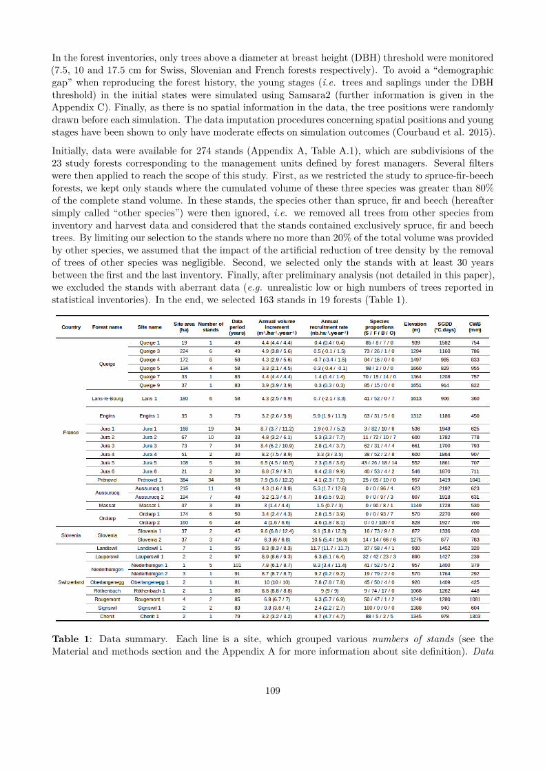
In the forest inventories, only trees above a diameter at breast height (DBH) threshold were monitored(7.5, 10 and 17.5 cm for Swiss, Slovenian and French forests respectively). To avoid a “demographicgap” when reproducing the forest history, the young stages (i.e. trees and saplings under the DBHthreshold) in the initial states were simulated using Samsara2 (further information is given in theAppendix C). Finally, as there is no spatial information in the data, the tree positions were randomlydrawn before each simulation. The data imputation procedures concerning spatial positions and youngstages have been shown to only have moderate efects on simulation outcomes (Courbaud et al. 2015).
Initially, data were available for 274 stands (Appendix A, Table A.1), which are subdivisions of the23 study forests corresponding to the management units deined by forest managers. Several ilterswere then applied to reach the scope of this study. First, as we restricted the study to spruce-ir-beechforests, we kept only stands where the cumulated volume of these three species was greater than 80%of the complete stand volume. In these stands, the species other than spruce, ir and beech (hereaftersimply called “other species”) were then ignored, i.e. we removed all trees from other species frominventory and harvest data and considered that the stands contained exclusively spruce, ir and beechtrees. By limiting our selection to the stands where no more than 20% of the total volume was providedby other species, we assumed that the impact of the artiicial reduction of tree density by the removalof trees of other species was negligible. Second, we selected only the stands with at least 30 yearsbetween the irst and the last inventory. Finally, after preliminary analysis (not detailed in this paper),we excluded the stands with aberrant data (e.g. unrealistic low or high numbers of trees reported instatistical inventories). In the end, we selected 163 stands in 19 forests (Table 1).
Table 1: Data summary. Each line is a site, which grouped various numbers of stands (see theMaterial and methods section and the Appendix A for more information about site deinition). Data
109
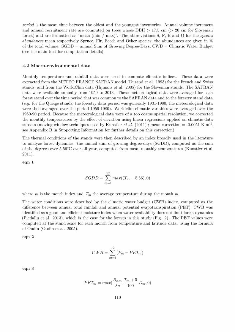
period is the mean time between the oldest and the youngest inventories. Annual volume incrementand annual recruitment rate are computed on trees whose DBH > 17.5 cm (> 20 cm for Slovenianforest) and are formatted as “mean (min / max)”. The abbreviations S, F, B and O for the speciesabundances mean respectively Spruce, Fir, Beech and Other species; the abundances are given in %of the total volume. SGDD = annual Sum of Growing Degree-Days; CWB = Climatic Water Budget(see the main text for computation details).
4.2 Macro-environmental data
Monthly temperature and rainfall data were used to compute climatic indices. These data wereextracted from the METEO FRANCE SAFRAN model (Durand et al. 1993) for the French and Swissstands, and from the WorldClim data (Hijmans et al. 2005) for the Slovenian stands. The SAFRANdata were available annually from 1959 to 2013. These meteorological data were averaged for eachforest stand over the time period that was common to the SAFRAN data and to the forestry stand data(e.g. for the Queige stands, the forestry data period was generally 1931-1980, the meteorological datawere then averaged over the period 1959-1980). Worldclim climatic variables were averaged over the1960-90 period. Because the meteorological data were of a too coarse spatial resolution, we correctedthe monthly temperatures by the efect of elevation using linear regressions applied on climatic datasubsets (moving window techniques used by Kunstler et al. (2011) ; mean correction = -0.0051 K.m-1,see Appendix B in Supporting Information for further details on this correction).
The thermal conditions of the stands were then described by an index broadly used in the literatureto analyze forest dynamics: the annual sum of growing degree-days (SGDD), computed as the sumof the degrees over 5.56°C over all year, computed from mean monthly temperatures (Kunstler et al.2011).
eqn 1
SGDD =12∑
m=1
max((Tm − 5.56), 0)
where m is the month index and Tm the average temperature during the month m.
The water conditions were described by the climatic water budget (CWB) index, computed as thediference between annual total rainfall and annual potential evapotranspiration (PET). CWB wasidentiied as a good and eicient moisture index when water availability does not limit forest dynamics(Piedallu et al. 2013), which is the case for the forests in this study (Fig. 2). The PET values werecomputed at the stand scale for each month from temperature and latitude data, using the formulaof Oudin (Oudin et al. 2005).
eqn 2
CWB =12∑
m=1
(Pm − PETm)
eqn 3
PETm = max(Re,m
λρ.Tm + 5
100.Dm, 0)
110
where Pm is the monthly sum of precipitation, Re,m is the extraterrestrial radiation (depending onmonth m), is the latent heat lux (taken equal to 2.45 MJ.kg-1), is the density of water (1000 kg.m-3)and Dm is the number of days in the month m. For further information about the computation of thediferent elements of this formula, please refer to Oudin et al. (2005) and Allen et al. (1998).
This simplistic PET formula may be questioned but, in the climatic area of our study, the Oudin PETvalues were highly correlated with the PET values computed with the formula of Penman (Penman1948), which is considered as the best approximation of PET. We used this formula because it allowedto correct PET as a function of elevation (using the temperature correction mentioned above) andthus to better segregate the forest stands close to each other.
As our main purpose was to analyze macro-climatic drivers over large gradients, we assumed that thevariations of forest dynamics were more determined by climate average conditions over time than byextreme climatic events, similarly to many species distribution models (Guisan and Thuiller 2005).After a brief analysis of the climate data, we also considered that climate conditions remained stableover time (in particular, we assumed that climate change was negligible over the 20th century), so thatwe could compare our forest stands despite the diferences in terms of time periods (period length,inventory dates). We checked that the length of data periods and the mean of inventory dates were notcorrelated with calibrated Samsara2 parameters (correlations were lower than 0.3 and not signiicantin all cases, see Table D.1 in Appendix D)
Finally, two other environmental variables were considered and computed at the stand scale: (1)temperature seasonality, deined as the standard deviation of monthly temperature over year, anindicator of intra-annual variability of temperature (and thus of thermal continentality) that can haveimportant efects on forest composition (Gauquelin and Courbaud 2006; Elkin et al. 2013); and (2)soil pH (pH), which is an important ecological factor for the study species (Piedallu et al. 2009). SoilpH data for French stands were provided by the LerFOB laboratory (Coudun et al. 2006), where itwas computed from the French Forest national inventory data by bio-indication. For the Slovenianstands, soil pH was provided with the historical data. The soil pH data were not available for theSwiss stands.
111
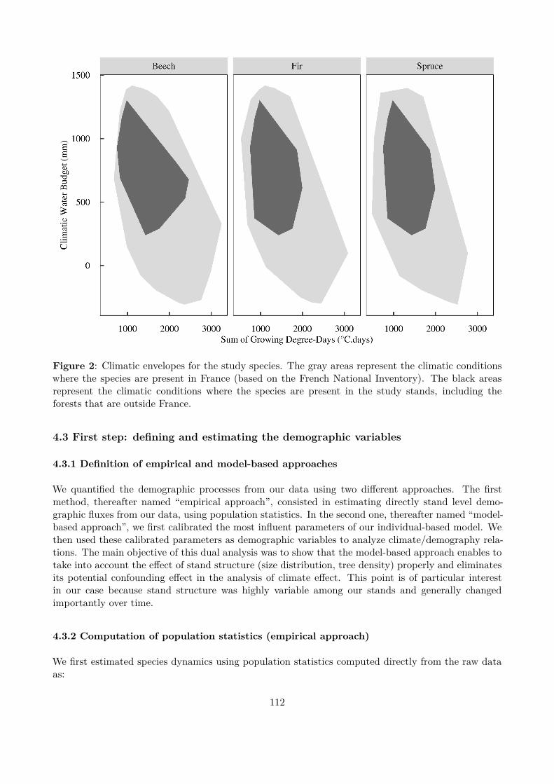
Figure 2: Climatic envelopes for the study species. The gray areas represent the climatic conditionswhere the species are present in France (based on the French National Inventory). The black areasrepresent the climatic conditions where the species are present in the study stands, including theforests that are outside France.
4.3 First step: deining and estimating the demographic variables
4.3.1 Deinition of empirical and model-based approaches
We quantiied the demographic processes from our data using two diferent approaches. The irstmethod, thereafter named “empirical approach”, consisted in estimating directly stand level demo-graphic luxes from our data, using population statistics. In the second one, thereafter named “model-based approach”, we irst calibrated the most inluent parameters of our individual-based model. Wethen used these calibrated parameters as demographic variables to analyze climate/demography rela-tions. The main objective of this dual analysis was to show that the model-based approach enables totake into account the efect of stand structure (size distribution, tree density) properly and eliminatesits potential confounding efect in the analysis of climate efect. This point is of particular interestin our case because stand structure was highly variable among our stands and generally changedimportantly over time.
4.3.2 Computation of population statistics (empirical approach)
We irst estimated species dynamics using population statistics computed directly from the raw dataas:
112
eqn 4
ΔVs = (volinit,s + volharv,s - volin,s) / period
where ΔV was an estimate of the annual volume increment; volinit, volharv and volin were the sum oftree volumes in the oldest inventory, the harvest data and the youngest inventory respectively; periodwas the number of years between the oldest and the youngest inventories, s stands for species. Onlythe trees with DBH above 17.5 cm (20 cm for Slovenian forest) were considered.
eqn 5
ΔNs = (ninit,s + nharv,s - nin,s) / period
where ΔN was an estimate of the species annual recruitment rate, i.e. the average number of treesreaching the DBH 17.5 cm (20 cm for Slovenian forest) each year; ninit, nharv and nin were thenumber of trees for the species in the oldest inventory, the harvest data and the youngest inventoryrespectively and period was the number of years between the oldest and the youngest inventories, sstands for species.
4.3.3 Calibration of the Samsara2 parameters (model-based approach)
Providing detailed information about the Samsara2 model and the calibration step is out of thescope of this study, as it was done elsewhere by Courbaud et al. (2015) and Lagarrigues et al.(2015) respectively. We nevertheless give here the key points about the Samsara2 model and thecalibration procedure. Samsara2 is an individual-based and spatially-explicit model developed tosimulate mountain forest dynamics (Courbaud et al. 2015). The demographic processes (tree growth,natural regeneration by germination and tree mortality) and the allometric equations used to deducethe key tree dimensions from DBH are modulated by species-speciic parameters (Vieilledent et al.2010). The initial objective of Samsara2 was to illuminate how forest stand dynamic patterns emergefrom the development of individual trees in competition for light, and in return, how the developmentof individual trees is controlled by stand structure manipulated by forest management. No otherenvironmental drivers than light (and in particular climate) are currently included explicitly in themodel.
Here are the main equations for the individual tree growth and regeneration processes, which are ofparticular interest in this study:
eqn 6
log(ΔGt,y,s(Et,y)) = log(GA,s + Gt,y,s) + GB,s * log(Et,y)
where ΔG is the tree basal area annual increment, GA and GB are species-speciic model parameters,E is the amount of light energy intercepted by the tree crown during the annual vegetation period andG is a random factor with a zero mean and a species-speciic variance, which varies with tree andyear to account for individual and annual variabilities of tree growth. The t, y and s subscripts meantree, year and species respectively.
eqn 7
Rc,y,s(Lc,y) = Pois(exp(RA,s)/100 . Sc,y,s(Lc,y))
where R is the annual regeneration (that is, the number of new saplings recruited in each 10 m x 10 mground cell), RA is the log-transformed potential number of saplings (species-speciic model parameter)and S is the survival rate, i.e. a number between 0 and 1 depending on species parameters and on theproportion of light reaching the ground cell during the considered year (L). The factor 100 is a scaled
113

factor, from stand (10,000 m2) to ground cell (100 m2). The S function is modeled by a bell-shapedresponse to light and is equal to 1 for an intermediate level of light, which difers between species.Pois stands for a random draw from a Poisson distribution.
Following the procedure detailed in Lagarrigues et al. (2015), we calibrated for each forest standtwo parameters per species, GA and RA, using an inverse modeling technique called ApproximateBayesian Computation (ABC). We used rather uninformative priors and ran 10,000 simulations foreach stand. We thus performed 1,630,000 simulations in total (10,000 simulations x 163 stands). Eachsimulation consisted in reproducing the stand historical dynamics and management, starting from theoldest inventory, and then by simulating successively natural dynamics and harvests as monitored inforestry data up to the date of the youngest inventory. The youngest inventory data was used asobservational data to estimate the joint posterior distributions of the species model parameters foreach stand independently. The modes of posterior distributions were then used as observational datafor the following analysis (see the next section). The slight modiications made in the method deinedby Lagarrigues et al. (2015) in the course of this study are detailed in the Appendix C.
The individual approach and the detailed modeling of light distribution among the diferent canopylayers used in the model Samsara2 enabled an explicit representation of the efect of stand structureon the light resource. The stand structure thus afected tree growth and regeneration indirectly bymodulating light conditions. For instance, the denser the stand, the less light is available for each tree(Et,y in Eq.6) and the less light reaches the ground and is available for seedlings (Lc,y in Eq.7). Thismain efect of stand structure being taken into account explicitly, we thus expected that the variationsof the estimates of the parameters (GA and RA) in diferent stands were little inluenced by standstructure and were mainly inluenced by other environmental factors.
Concerning the regeneration process, the RA parameter represented the number of saplings potentiallyrecruited as adult trees (i.e. once they reach the DBH 7.5 cm) at optimal light conditions after initialreduction due to ground light conditions. Seedling growth spanned over several years in the modelbefore recruitment occurred but seedling mortality caused by non optimal ground light conditionswas collapsed into a single event at the same time than germination (Eq. 7). The parameter RArepresented thus more the renewal of adult trees (i.e. the number of saplings that will reach the adultstage) than a realistic number of saplings. This relative simple representation of the regenerationprocess was necessary in this study since our data give only information about adult trees and a moresophisticated representation of sapling dynamics can hardly be calibrated with such data.
Regarding the relations to environmental factors, as the RA parameter synthesizes the potential re-cruitment over long periods (from installation to recruitment), we made the assumption that it wouldbe more sensitive to average climate conditions than to extreme events.
4.4 Second step: quantifying the relations between the demographic and the macro-environmental variables
4.4.1 Site deinition
From this step on, the stands were grouped in sites. The motivation for this aggregation was thatsome forest inventories were based on statistical sampling, with few points at the stand scale (typically,10 samples in a stand of 10 ha), making the estimates of the demographic variables more robuststatistically at the site scale. Basically, the sites corresponded to forests, except for the large forestsencompassing a large altitudinal gradient, which were further divided into multiple sites in order tohave homogeneous climatic conditions within sites. This site deinition was performed using formalclustering techniques and qualitative considerations (detailed in Appendix A). 31 sites were accordingly
114

deined, they are listed in Table 1 and the stand characteristics are detailed in the Table A.1 (AppendixA). The site-level population statistics and the environmental variables were computed by averagingthe stand-level values. The calibrated parameters for a given site were computed by merging thestand-scale posterior distributions and then by taking the mode of the global distribution.
4.4.2 Multiple linear regressions
We carried out regressions between demographic and environmental variables using site-level data. Weused multiple linear models, independently for each demographic process (growth and regeneration)and species (spruce, ir and beech), applied irst on the population statistics and then on the Samsara2parameters (i.e. twelve independent models in total). We assumed that the site dynamics wereindependent from each other and we ignored possible spatial autocorrelations. We used the annualsum of growing degree-days (SGDD), the climatic water budget (CWB), the temperature seasonalityand the soil pH as explicative variables. We checked that these factors were not correlated with eachother (see Appendix D). In addition to these environmental variables, we added an endogenous factor,namely average species basal area, which was computed as the mean of species basal area between theoldest and the youngest inventories.
We added quadratic terms for SGDD and CWB. Quadratic responses of tree growth to these factorshave been questioned recently in conditions where thermal or water conditions are limiting (Bugmannand Solomon 2000). However, as we did not study the extreme conditions for our species on thesetwo environmental axes, we considered that the left hand side of a second-degree polynomial responsecurve was a good approximation.
We applied a procedure of model selection based on the AIC criterion and included only the parsimo-nious set of signiicant variables in the inal results.
115
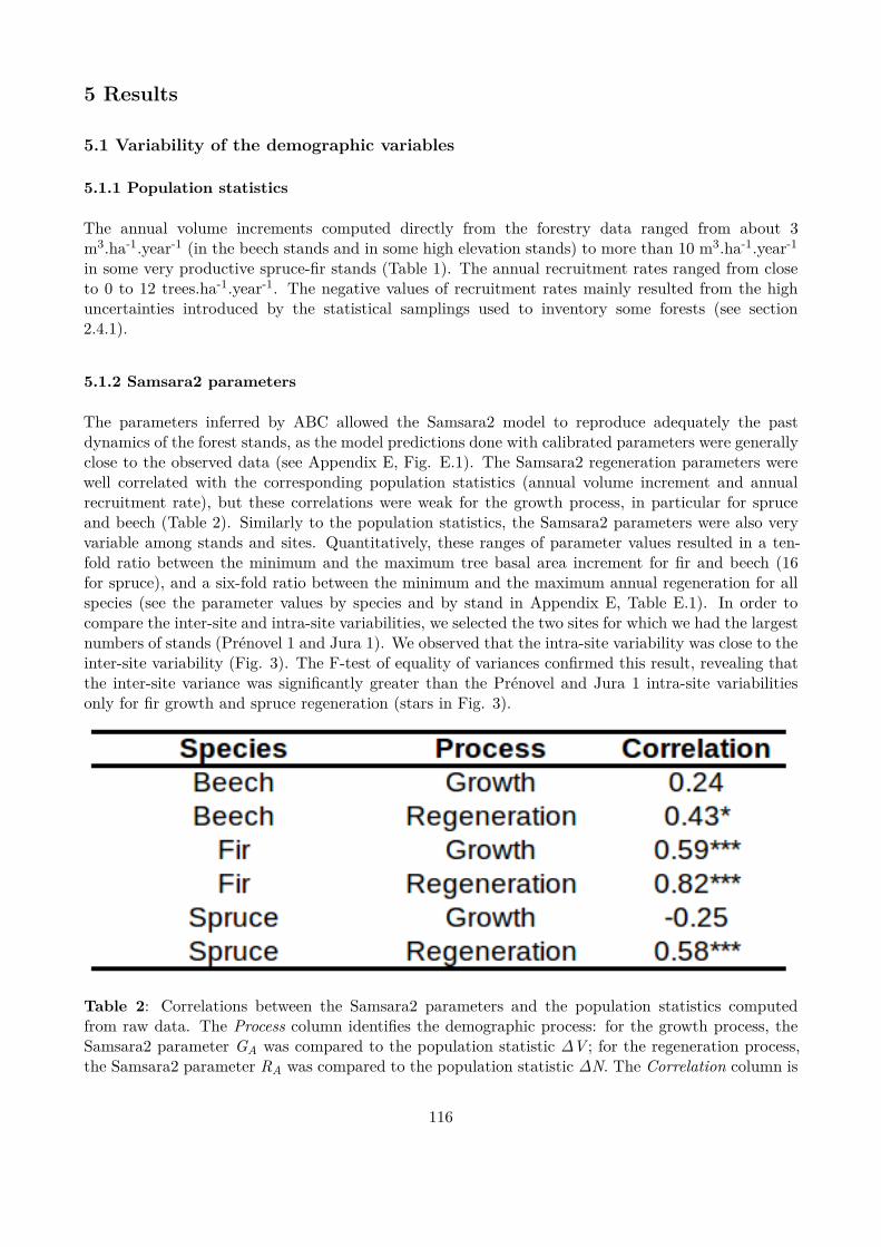
5 Results
5.1 Variability of the demographic variables
5.1.1 Population statistics
The annual volume increments computed directly from the forestry data ranged from about 3m3.ha-1.year-1 (in the beech stands and in some high elevation stands) to more than 10 m3.ha-1.year-1
in some very productive spruce-ir stands (Table 1). The annual recruitment rates ranged from closeto 0 to 12 trees.ha-1.year-1. The negative values of recruitment rates mainly resulted from the highuncertainties introduced by the statistical samplings used to inventory some forests (see section2.4.1).
5.1.2 Samsara2 parameters
The parameters inferred by ABC allowed the Samsara2 model to reproduce adequately the pastdynamics of the forest stands, as the model predictions done with calibrated parameters were generallyclose to the observed data (see Appendix E, Fig. E.1). The Samsara2 regeneration parameters werewell correlated with the corresponding population statistics (annual volume increment and annualrecruitment rate), but these correlations were weak for the growth process, in particular for spruceand beech (Table 2). Similarly to the population statistics, the Samsara2 parameters were also veryvariable among stands and sites. Quantitatively, these ranges of parameter values resulted in a ten-fold ratio between the minimum and the maximum tree basal area increment for ir and beech (16for spruce), and a six-fold ratio between the minimum and the maximum annual regeneration for allspecies (see the parameter values by species and by stand in Appendix E, Table E.1). In order tocompare the inter-site and intra-site variabilities, we selected the two sites for which we had the largestnumbers of stands (Prénovel 1 and Jura 1). We observed that the intra-site variability was close to theinter-site variability (Fig. 3). The F-test of equality of variances conirmed this result, revealing thatthe inter-site variance was signiicantly greater than the Prénovel and Jura 1 intra-site variabilitiesonly for ir growth and spruce regeneration (stars in Fig. 3).
Table 2: Correlations between the Samsara2 parameters and the population statistics computedfrom raw data. The Process column identiies the demographic process: for the growth process, theSamsara2 parameter GA was compared to the population statistic ΔV ; for the regeneration process,the Samsara2 parameter RA was compared to the population statistic ΔN. The Correlation column is
116
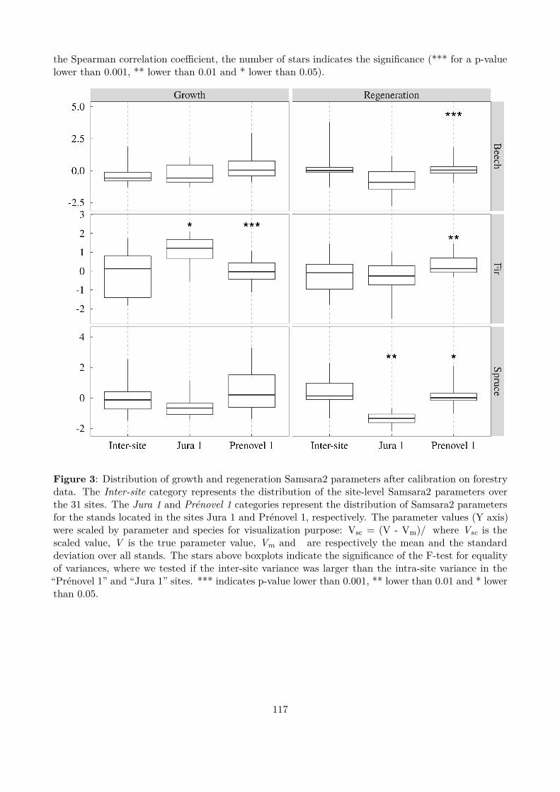
the Spearman correlation coeicient, the number of stars indicates the signiicance (*** for a p-valuelower than 0.001, ** lower than 0.01 and * lower than 0.05).
Figure 3: Distribution of growth and regeneration Samsara2 parameters after calibration on forestrydata. The Inter-site category represents the distribution of the site-level Samsara2 parameters overthe 31 sites. The Jura 1 and Prénovel 1 categories represent the distribution of Samsara2 parametersfor the stands located in the sites Jura 1 and Prénovel 1, respectively. The parameter values (Y axis)were scaled by parameter and species for visualization purpose: Vsc = (V - Vm)/ where Vsc is thescaled value, V is the true parameter value, Vm and are respectively the mean and the standarddeviation over all stands. The stars above boxplots indicate the signiicance of the F-test for equalityof variances, where we tested if the inter-site variance was larger than the intra-site variance in the“Prénovel 1” and “Jura 1” sites. *** indicates p-value lower than 0.001, ** lower than 0.01 and * lowerthan 0.05.
117
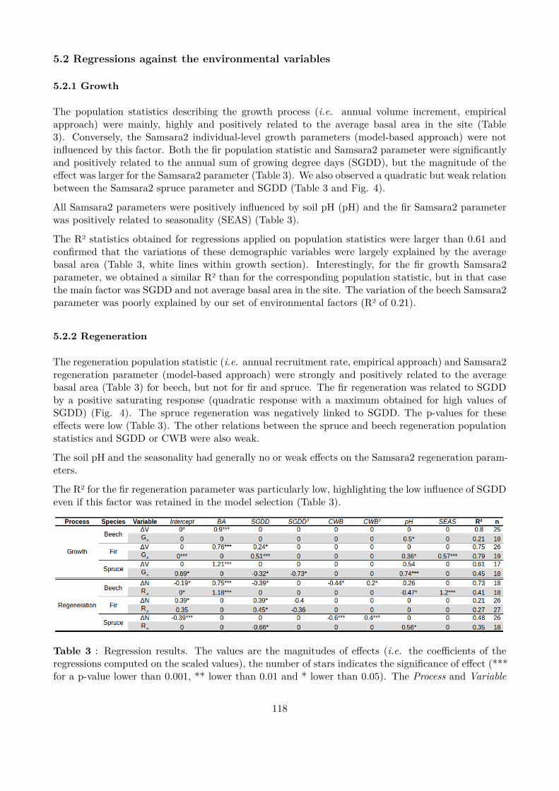
5.2 Regressions against the environmental variables
5.2.1 Growth
The population statistics describing the growth process (i.e. annual volume increment, empiricalapproach) were mainly, highly and positively related to the average basal area in the site (Table3). Conversely, the Samsara2 individual-level growth parameters (model-based approach) were notinluenced by this factor. Both the ir population statistic and Samsara2 parameter were signiicantlyand positively related to the annual sum of growing degree days (SGDD), but the magnitude of theefect was larger for the Samsara2 parameter (Table 3). We also observed a quadratic but weak relationbetween the Samsara2 spruce parameter and SGDD (Table 3 and Fig. 4).
All Samsara2 parameters were positively inluenced by soil pH (pH) and the ir Samsara2 parameterwas positively related to seasonality (SEAS) (Table 3).
The R² statistics obtained for regressions applied on population statistics were larger than 0.61 andconirmed that the variations of these demographic variables were largely explained by the averagebasal area (Table 3, white lines within growth section). Interestingly, for the ir growth Samsara2parameter, we obtained a similar R² than for the corresponding population statistic, but in that casethe main factor was SGDD and not average basal area in the site. The variation of the beech Samsara2parameter was poorly explained by our set of environmental factors (R² of 0.21).
5.2.2 Regeneration
The regeneration population statistic (i.e. annual recruitment rate, empirical approach) and Samsara2regeneration parameter (model-based approach) were strongly and positively related to the averagebasal area (Table 3) for beech, but not for ir and spruce. The ir regeneration was related to SGDDby a positive saturating response (quadratic response with a maximum obtained for high values ofSGDD) (Fig. 4). The spruce regeneration was negatively linked to SGDD. The p-values for theseefects were low (Table 3). The other relations between the spruce and beech regeneration populationstatistics and SGDD or CWB were also weak.
The soil pH and the seasonality had generally no or weak efects on the Samsara2 regeneration param-eters.
The R² for the ir regeneration parameter was particularly low, highlighting the low inluence of SGDDeven if this factor was retained in the model selection (Table 3).
Table 3 : Regression results. The values are the magnitudes of efects (i.e. the coeicients of theregressions computed on the scaled values), the number of stars indicates the signiicance of efect (***for a p-value lower than 0.001, ** lower than 0.01 and * lower than 0.05). The Process and Variable
118
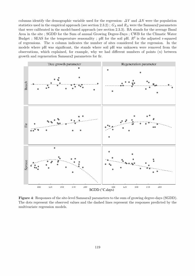
columns identify the demographic variable used for the regression: ΔV and ΔN were the populationstatistics used in the empirical approach (see section 2.3.2) ; GA and RA were the Samsara2 parametersthat were calibrated in the model-based approach (see section 2.3.3). BA stands for the average BasalArea in the site ; SGDD for the Sum of annual Growing Degree-Days ; CWB for the Climatic WaterBudget ; SEAS for the temperature seasonality ; pH for the soil pH. R2 is the adjusted r-squaredof regressions. The n column indicates the number of sites considered for the regression. In themodels where pH was signiicant, the stands where soil pH was unknown were removed from theobservations, which explained, for example, why we had diferent numbers of points (n) betweengrowth and regeneration Samsara2 parameters for ir.
Figure 4: Responses of the site-level Samsara2 parameters to the sum of growing degree-days (SGDD).The dots represent the observed values and the dashed lines represent the responses predicted by themultivariate regression models.
119
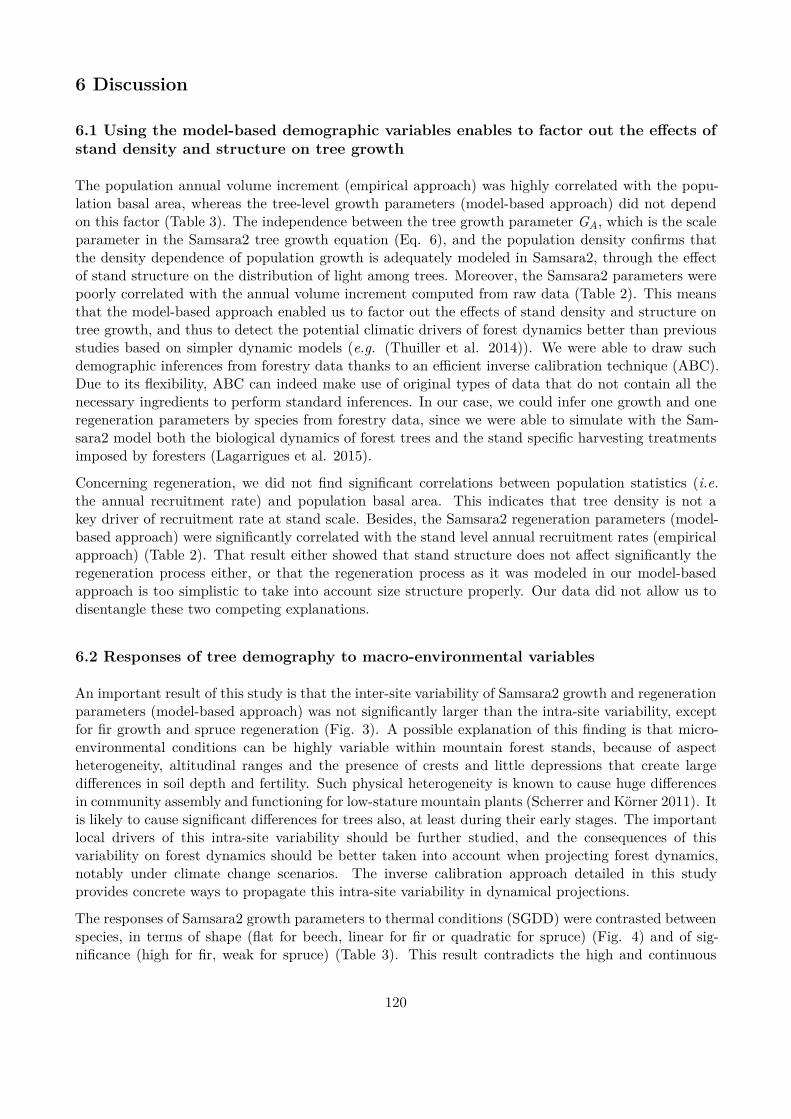
6 Discussion
6.1 Using the model-based demographic variables enables to factor out the efects ofstand density and structure on tree growth
The population annual volume increment (empirical approach) was highly correlated with the popu-lation basal area, whereas the tree-level growth parameters (model-based approach) did not dependon this factor (Table 3). The independence between the tree growth parameter GA, which is the scaleparameter in the Samsara2 tree growth equation (Eq. 6), and the population density conirms thatthe density dependence of population growth is adequately modeled in Samsara2, through the efectof stand structure on the distribution of light among trees. Moreover, the Samsara2 parameters werepoorly correlated with the annual volume increment computed from raw data (Table 2). This meansthat the model-based approach enabled us to factor out the efects of stand density and structure ontree growth, and thus to detect the potential climatic drivers of forest dynamics better than previousstudies based on simpler dynamic models (e.g. (Thuiller et al. 2014)). We were able to draw suchdemographic inferences from forestry data thanks to an eicient inverse calibration technique (ABC).Due to its lexibility, ABC can indeed make use of original types of data that do not contain all thenecessary ingredients to perform standard inferences. In our case, we could infer one growth and oneregeneration parameters by species from forestry data, since we were able to simulate with the Sam-sara2 model both the biological dynamics of forest trees and the stand speciic harvesting treatmentsimposed by foresters (Lagarrigues et al. 2015).
Concerning regeneration, we did not ind signiicant correlations between population statistics (i.e.the annual recruitment rate) and population basal area. This indicates that tree density is not akey driver of recruitment rate at stand scale. Besides, the Samsara2 regeneration parameters (model-based approach) were signiicantly correlated with the stand level annual recruitment rates (empiricalapproach) (Table 2). That result either showed that stand structure does not afect signiicantly theregeneration process either, or that the regeneration process as it was modeled in our model-basedapproach is too simplistic to take into account size structure properly. Our data did not allow us todisentangle these two competing explanations.
6.2 Responses of tree demography to macro-environmental variables
An important result of this study is that the inter-site variability of Samsara2 growth and regenerationparameters (model-based approach) was not signiicantly larger than the intra-site variability, exceptfor ir growth and spruce regeneration (Fig. 3). A possible explanation of this inding is that micro-environmental conditions can be highly variable within mountain forest stands, because of aspectheterogeneity, altitudinal ranges and the presence of crests and little depressions that create largediferences in soil depth and fertility. Such physical heterogeneity is known to cause huge diferencesin community assembly and functioning for low-stature mountain plants (Scherrer and Körner 2011). Itis likely to cause signiicant diferences for trees also, at least during their early stages. The importantlocal drivers of this intra-site variability should be further studied, and the consequences of thisvariability on forest dynamics should be better taken into account when projecting forest dynamics,notably under climate change scenarios. The inverse calibration approach detailed in this studyprovides concrete ways to propagate this intra-site variability in dynamical projections.
The responses of Samsara2 growth parameters to thermal conditions (SGDD) were contrasted betweenspecies, in terms of shape (lat for beech, linear for ir or quadratic for spruce) (Fig. 4) and of sig-niicance (high for ir, weak for spruce) (Table 3). This result contradicts the high and continuous
120
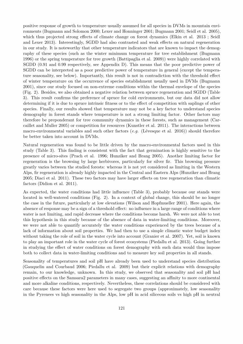
positive response of growth to temperature usually assumed for all species in DVMs in mountain envi-ronments (Bugmann and Solomon 2000; Lexer and Honninger 2001; Bugmann 2001; Seidl et al. 2005),which thus projected strong efects of climate change on forest dynamics (Elkin et al. 2013 ; Seidland Lexer 2013). Interestingly, SGDD had also contrasted and weak efects on natural regenerationin our study. It is noteworthy that other temperature indicators that are known to impact the demog-raphy of these species (such as the winter minimum temperature for tree establishment (Bugmann1996) or the spring temperature for tree growth (Battipaglia et al. 2009)) were highly correlated withSGDD (0.91 and 0.99 respectively, see Appendix D). This means that the poor predictive power ofSGDD can be interpreted as a poor predictive power of temperature in general (except the tempera-ture seasonality, see below). Importantly, this result is not in contradiction with the threshold efectof winter temperature on the occurrence of species establishment usually used in DVMs (Bugmann2001), since our study focused on non-extreme conditions within the thermal envelope of the species(Fig. 2). Besides, we also obtained a negative relation between spruce regeneration and SGDD (Table3). This result conirms the preference of spruce for cold environments, but our data did not allowdetermining if it is due to spruce intrinsic itness or to the efect of competition with saplings of otherspecies. Finally, our results showed that temperature may not be a key factor to understand speciesdemography in forest stands where temperature is not a strong limiting factor. Other factors maytherefore be preponderant for tree community dynamics in these forests, such as management (Car-caillet and Muller 2005) or competition for resources (Kunstler et al. 2011). The interactions betweenmacro-environmental variables and such other factors (e.g. (Lévesque et al. 2016)) should thereforebe better taken into account in DVMs.
Natural regeneration was found to be little driven by the macro-environmental factors used in thisstudy (Table 3). This inding is consistent with the fact that germination is highly sensitive to thepresence of micro-sites (Prach et al. 1996; Hunziker and Brang 2005). Another limiting factor forregeneration is the browsing by large herbivores, particularly for silver ir. This browsing pressuregreatly varies between the studied forests: whereas it is not yet considered as limiting in the WesternAlps, ir regeneration is already highly impacted in the Central and Eastern Alps (Hunziker and Brang2005; Diaci et al. 2011). These two factors may have larger efects on tree regeneration than climaticfactors (Didion et al. 2011).
As expected, the water conditions had little inluence (Table 3), probably because our stands werelocated in well-watered conditions (Fig. 2). In a context of global change, this should be no longerthe case in the future, particularly at low elevations (Wilson and Hopfmueller 2001). Here again, theabsence of response may be a sign of a threshold efect: no inluence in a large range of conditions wherewater is not limiting, and rapid decrease where the conditions become harsh. We were not able to testthis hypothesis in this study because of the absence of data in water-limiting conditions. Moreover,we were not able to quantify accurately the water conditions experienced by the trees because of alack of information about soil properties. We had then to use a simple climatic water budget indexwithout taking the role of soil in the water cycle into account (Granier et al. 2007). Yet, soil is knownto play an important role in the water cycle of forest ecosystems (Piedallu et al. 2013). Going furtherin studying the efect of water conditions on forest demography with such data would thus imposeboth to collect data in water-limiting conditions and to measure key soil properties in all stands.
Seasonality of temperatures and soil pH have already been used to understand species distribution(Gauquelin and Courbaud 2006; Piedallu et al. 2009) but their explicit relations with demographyremain, to our knowledge, unknown. In this study, we observed that seasonality and soil pH hadpositive efects on the Samsara2 parameters in many cases, suggesting an ainity to more continentaland more alkaline conditions, respectively. Nevertheless, these correlations should be considered withcare because these factors were here used to segregate two groups (approximately, low seasonalityin the Pyrenees vs high seasonality in the Alps, low pH in acid siliceous soils vs high pH in neutral
121

calcareous soils), with a very low variability inside these groups as compared to the gaps occurringbetween groups (Table A.1 in Appendix A and Fig. D.1 in Appendix D). These relations should thusbe investigated with a better sample of sites along these factors.
6.3 The potential of forestry data for ecological research
This study relied on data mainly collected by forest managers to monitor the evolution of their forestsrather than on research data. Considering the data scarcity in forest ecology, these forestry data areuseful to quantify forest dynamics along large environmental gradients. In particular, an importantadded value of these long term data (up to 100 years of forest dynamics) is to allow the quantiicationof the renewal of forest stands by means of natural regeneration. Indeed, the lack of long-term data isoften an important limit to predict the future species dynamics in forest stands (Piedallu et al. 2009;Snell et al. 2014). Besides, this data source is far from being completely exploited with this study: further information can likely be extracted from the present data set (e.g. to study the mortalityprocess (Csillery et al. 2013)) and management documents are available for many other forests acrossEurope. Thanks to modern inference techniques such as ABC, forestry data give critical informationabout the long-term forest dynamics in a warming climate, and should therefore be more widelycompiled and used for global change research.
122

7 Acknowledgment
We thank all data providers, in particular the French Forest National Oice for its assistance whileextracting data from their archives. The data compilation for the Slovenian stands, done by theUniversity of Ljubljana, was funded by the European FP7 research project “Advanced multifunctionalforest management in European mountain ranges” (ARANGE, n° 289437). The simulations werecarried out using the computing center CIMENT located in the Grenoble University and we thank theCIMENT supporting team and Eric Maldonado from IRSTEA Grenoble for their help to ix technicalissues related to the use of the simulation platform. Guillaume Lagarrigues was funded by the FrenchEnvironment and Energy Management Agency (ADEME), the French Forest National Oice (ONF)and IRSTEA. IRSTEA Grenoble is a part of labex OSUG@2020. We have no conlicts of interest todisclose.
123

8 Data accessibility
• Forestry and environmental data : will be stored in Dryad• Samsara2 model source code : available in the Capsis platform (Dufour-Kowalski et al. 2012)
(http://capsis.cirad.fr/), with restricted access• R scripts : uploaded as online supporting information
124

9 Supporting information
Additional supporting information may be found in the online version of this article:
• Appendix A : Stand and site features• Appendix B : Temperature correction in function of elevation• Appendix C : Speciic recalibration features for this study• Appendix D : Correlations between environmental variables• Appendix E : Detailed results of the recalibration step
125
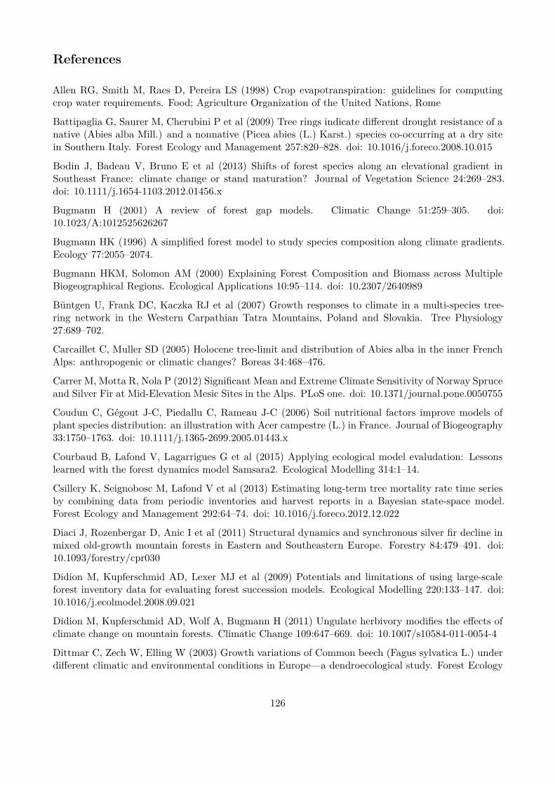
References
Allen RG, Smith M, Raes D, Pereira LS (1998) Crop evapotranspiration: guidelines for computingcrop water requirements. Food; Agriculture Organization of the United Nations, Rome
Battipaglia G, Saurer M, Cherubini P et al (2009) Tree rings indicate diferent drought resistance of anative (Abies alba Mill.) and a nonnative (Picea abies (L.) Karst.) species co-occurring at a dry sitein Southern Italy. Forest Ecology and Management 257:820–828. doi: 10.1016/j.foreco.2008.10.015
Bodin J, Badeau V, Bruno E et al (2013) Shifts of forest species along an elevational gradient inSoutheast France: climate change or stand maturation? Journal of Vegetation Science 24:269–283.doi: 10.1111/j.1654-1103.2012.01456.x
Bugmann H (2001) A review of forest gap models. Climatic Change 51:259–305. doi:10.1023/A:1012525626267
Bugmann HK (1996) A simpliied forest model to study species composition along climate gradients.Ecology 77:2055–2074.
Bugmann HKM, Solomon AM (2000) Explaining Forest Composition and Biomass across MultipleBiogeographical Regions. Ecological Applications 10:95–114. doi: 10.2307/2640989
Büntgen U, Frank DC, Kaczka RJ et al (2007) Growth responses to climate in a multi-species tree-ring network in the Western Carpathian Tatra Mountains, Poland and Slovakia. Tree Physiology27:689–702.
Carcaillet C, Muller SD (2005) Holocene tree-limit and distribution of Abies alba in the inner FrenchAlps: anthropogenic or climatic changes? Boreas 34:468–476.
Carrer M, Motta R, Nola P (2012) Signiicant Mean and Extreme Climate Sensitivity of Norway Spruceand Silver Fir at Mid-Elevation Mesic Sites in the Alps. PLoS one. doi: 10.1371/journal.pone.0050755
Coudun C, Gégout J-C, Piedallu C, Rameau J-C (2006) Soil nutritional factors improve models ofplant species distribution: an illustration with Acer campestre (L.) in France. Journal of Biogeography33:1750–1763. doi: 10.1111/j.1365-2699.2005.01443.x
Courbaud B, Lafond V, Lagarrigues G et al (2015) Applying ecological model evaludation: Lessonslearned with the forest dynamics model Samsara2. Ecological Modelling 314:1–14.
Csillery K, Seignobosc M, Lafond V et al (2013) Estimating long-term tree mortality rate time seriesby combining data from periodic inventories and harvest reports in a Bayesian state-space model.Forest Ecology and Management 292:64–74. doi: 10.1016/j.foreco.2012.12.022
Diaci J, Rozenbergar D, Anic I et al (2011) Structural dynamics and synchronous silver ir decline inmixed old-growth mountain forests in Eastern and Southeastern Europe. Forestry 84:479–491. doi:10.1093/forestry/cpr030
Didion M, Kupferschmid AD, Lexer MJ et al (2009) Potentials and limitations of using large-scaleforest inventory data for evaluating forest succession models. Ecological Modelling 220:133–147. doi:10.1016/j.ecolmodel.2008.09.021
Didion M, Kupferschmid AD, Wolf A, Bugmann H (2011) Ungulate herbivory modiies the efects ofclimate change on mountain forests. Climatic Change 109:647–669. doi: 10.1007/s10584-011-0054-4
Dittmar C, Zech W, Elling W (2003) Growth variations of Common beech (Fagus sylvatica L.) underdiferent climatic and environmental conditions in Europe—a dendroecological study. Forest Ecology
126
and Management 63–78.
Dufour-Kowalski S, Courbaud B, Dreyfus P et al (2012) Capsis: an open software framework andcommunity for forest growth modelling. Annals of Forest Science 69:221–233.
Durand Y, Brun E, Mérindol L et al (1993) A meteorological estimation of relevant parameters forsnow models. Annals of Glaciology 18:65–71.
Elkin C, Giuggiola A, Rigling A, Bugmann H (2015) Short- and long-term eicacy of forest thinning tomitigate drought impacts in mountain forests in the European Alps. Ecological Applications 25:1083–1098. doi: 10.1890/14-0690.1
Elkin C, Gutiérrez AG, Leuzinger S et al (2013) A 2 °C warmer world is not safe for ecosystem servicesin the European Alps. Global Change Biology 19:1827–1840. doi: 10.1111/gcb.12156
Fontes L, Bontemps JD, Bugmann H et al (2010) Models for supporting forest management in achanging environment. Forest Systems 19:8–29.
Gauquelin X, Courbaud B (2006) Guide des sylvicultures de montagne. ONF/CRPF/Cemagref
Granier A, Reichstein M, Bréda N et al (2007) Evidence for soil water control on carbon and water dy-namics in European forests during the extremely dry year: 2003. Agricultural and Forest Meteorology143:123–145. doi: 10.1016/j.agrformet.2006.12.004
Grassi G, Minotta G, Tonon G, Bagnaresi U (2004) Dynamics of Norway spruce and silver ir naturalregeneration in a mixed stand under uneven-aged management. Canadian Journal of Forest Research-Revue Canadienne De Recherche Forestiere 34:141–149. doi: 10.1139/x03-197
Guisan A, Thuiller W (2005) Predicting species distribution: ofering more than simple habitat models.Ecology Letters 8:993–1009. doi: 10.1111/j.1461-0248.2005.00792.x
Hanewinkel M, Cullmann DA, Schelhaas M-J et al (2013) Climate change may cause severe loss inthe economic value of European forest land. Nature Climate Change 3:203–207. doi: 10.1038/ncli-mate1687
Hartig F, Dyke J, Hickler T et al (2012) Connecting dynamic vegetation models to data - an inverseperspective. Journal of Biogeography 39:2240–2252. doi: 10.1111/j.1365-2699.2012.02745.x
Hickler T, Vohland K, Feehan J et al (2012) Projecting the future distribution of European potentialnatural vegetation zones with a generalized, tree species-based dynamic vegetation model. GlobalEcology and Biogeography 21:50–63. doi: 10.1111/j.1466-8238.2010.00613.x
Hijmans RJ, Cameron SE, Parra JL et al (2005) Very high resolution interpolated climate surfacesfor global land areas. International journal of climatology 25:1965–1978.
Hunziker U, Brang P (2005) Microsite patterns of conifer seedling establishment and growth in amixed stand in the southern Alps. Forest Ecology and Management 210:67–79.
Keenan RJ (2015) Climate change impacts and adaptation in forest management: a review. Annalsof Forest Science 72:145–167.
Klopcic M, Jerina K, Boncina A (2010) Long-term changes of structure and tree species composition inDinaric uneven-aged forests: are red deer an important factor? European Journal of Forest Research129:277–288. doi: 10.1007/s10342-009-0325-z
Körner C, Basler D, Hoch G et al (2016) Where, why and how? Explaining the low-temperature range
127
limits of temperate tree species. Journal of Ecology 104:1076–1088. doi: 10.1111/1365-2745.12574
Kunstler G, Albert CH, Courbaud B et al (2011) Efects of competition on tree radial-growth vary inimportance but not in intensity along climatic gradients. Journal of Ecology 99:300–312.
Lagarrigues G, Jabot F, Lafond V, Courbaud B (2015) Approximate Bayesian computation to re-calibrate individual-based models with population data: Illustration with a forest simulation model.Ecological Modelling 306:278–286.
Lenoir J, Gégout J-C, Pierrat J-C et al (2009) Diferences between tree species seedling and adultaltitudinal distribution in mountain forests during the recent warm period (1986-2006). Ecography32:765–777.
Lexer MJ, Honninger K (2001) A modiied 3D-patch model for spatially explicit simulation of veg-etation composition in heterogeneous landscapes. Forest Ecology and Management 144:43–65. doi:10.1016/s0378-1127(00)00386-8
Lévesque M, Walthert L, Weber P (2016) Soil nutrients inluence growth response of temperate treespecies to drought. Journal of Ecology 104:377–387. doi: 10.1111/1365-2745.12519
Lindner M, Fitzgerald JB, Zimmermann NE et al (2014) Climate change and European forests: Whatdo we know, what are the uncertainties, and what are the implications for forest management? Journalof environmental management 146:69–83.
Mäkinen H, Nöjd P, Kahle HP et al (2002) Radial growth variation of Norway spruce (Picea abies (L.)Karst.) across latitudinal and altitudinal gradients in central and northern Europe. Forest Ecologyand Management 171:243–259.
Mencuccini M, Piussi P, Zanzi Sulli A (1995) Thirty years of seed production in a subalpine Norwayspruce forest: patterns of temporal and spatial variation. Forest Ecology and Management 76:109–125.doi: 10.1016/0378-1127(95)03555-O
Oudin L, Hervieu F, Michel C et al (2005) Which potential evapotranspiration input for a lumpedrainfall–runof model?: Part 2—Towards a simple and eicient potential evapotranspiration model forrainfall–runof modelling. Journal of Hydrology 303:290–306.
Paluch JG, Jastrzębski R (2013) Natural regeneration of shade-tolerant Abies alba Mill. in gradientsof stand species compositions: Limitation by seed availability or safe microsites? Forest Ecology andManagement 307:322–332.
Penman HL (1948) Natural Evaporation from Open Water, Bare Soil and Grass. Proceedings ofthe Royal Society of London A: Mathematical, Physical and Engineering Sciences 193:120–145. doi:10.1098/rspa.1948.0037
Piedallu C, Gégout J-C, Perez V, Lebourgeois F (2013) Soil water balance performs better thanclimatic water variables in tree species distribution modelling. Global Ecology and Biogeography22:470–482.
Piedallu C, Perez V, Gégout J-C et al (2009) Impact potentiel du changement climatique sur ladistribution de l’Epicéa, du Sapin, du Hêtre et du Chêne sessile en France. Revue forestière française61:567–593.
Pinto PE, Gégout J-C, Hervé J-C, Dhôte J-F (2008) Respective importance of ecological conditionsand stand composition on Abies alba Mill. dominant height growth. Forest Ecology and Management255:619–629. doi: 10.1016/j.foreco.2007.09.031
Prach K, Lepš J, Michálek J (1996) Establishment of Picea abies Seedlings in a Central Euro-
128

pean Mountain Grassland: An Experimental Study. Journal of Vegetation Science 7:681–684. doi:10.2307/3236379
Rolland C, Petitcolas V, Michalet R (1998) Changes in radial tree growth for Picea abies, Larixdecidua, Pinus cembra and Pinus uncinata near the alpine timberline since 1750. Trees 13:40–53.
Scheiter S, Langan L, Higgins SI (2013) Next-generation dynamic global vegetation models: learningfrom community ecology. New Phytologist 198:957–969. doi: 10.1111/nph.12210
Scherrer D, Körner C (2011) Topographically controlled thermal-habitat diferentiation bufers alpineplant diversity against climate warming. Journal of Biogeography 38:406–416. doi: 10.1111/j.1365-2699.2010.02407.x
Seidl R, Lexer MJ (2013) Forest management under climatic and social uncertainty: Trade-ofs be-tween reducing climate change impacts and fostering adaptive capacity. Journal of EnvironmentalManagement 114:461–469.
Seidl R, Lexer MJ, Jäger D, Hönninger K (2005) Evaluating the accuracy and generality of a hybridpatch model. Tree Physiology 25:939–951. doi: 10.1093/treephys/25.7.939
Selås V, Piovesan G, Adams JM, Bernabei M (2002) Climatic factors controlling reproduction andgrowth of Norway spruce in southern Norway. Canadian Journal of Forest Research 32:217–225. doi:10.1139/x01-192
Seynave I, Gegout J-C, Herve J-C, Dhote J-F (2008) Is the spatial distribution of European beech(Fagus sylvatica L.) limited by its potential height growth? Journal of Biogeography 35:1851–1862.doi: 10.1111/j.1365-2699.2008.01930.x
Snell R, Huth A, Nabel J et al (2014) Using dynamic vegetation models to simulate plant range shifts.Ecography 37:1184–1197.
Stancioiu PT, O’Hara KL (2006) Regeneration growth in diferent light environments of mixed species,multiaged, mountainous forests of Romania. European Journal of Forest Research 125:151–162. doi:10.1007/s10342-005-0069-3
Tegel W, Seim A, Hakelberg D et al (2014) A recent growth increase of European beech (Fagussylvatica L.) at its Mediterranean distribution limit contradicts drought stress. European Journal ofForest Research 133:61–71.
Thuiller W, Münkemüller T, Schifers KH et al (2014) Does probability of occurrence relate to popu-lation dynamics? Ecography 37:1155–1166.
Tinner W, Colombaroli D, Heiri O et al (2013) The past ecology of Abies alba provides new perspectiveson future responses of silver ir forests to global warming. Ecological Monographs 83:419–439.
Vieilledent G, Courbaud B, Kunstler G et al (2010) Individual variability in tree allometry determineslight resource allocation in forest ecosystems: a hierarchical Bayesian approach. Oecologia 163:759–773. doi: 10.1007/s00442-010-1581-9
Wang WJ, He HS, Spetich MA et al (2013) A large-scale forest landscape model incorporating multi-scale processes and utilizing forest inventory data. Ecosphere. doi: 10.1890/es13-00040.1
Wilson RJ, Hopfmueller M (2001) Dendrochronological investigations of Norway spruce along anelevational transect in the Bavarian Forest, Germany. Dendrochronologia 19:67–79.
Wisz MS, Pottier J, Kissling WD et al (2013) The role of biotic interactions in shaping distributionsand realised assemblages of species: implications for species distribution modelling. Biological Reviews
129

of the Cambridge Philosophical Society 88:15–30. doi: 10.1111/j.1469-185X.2012.00235.x
Zingg A, Frutig F, Bürgi A et al (2009) Yield performance in the plenter forest research plots inSwitzerland. Dauerwald 160:162–174. doi: 10.3188/szf.2009.0162
130

Supplementary information for manuscript‘Demographic variability in spruce-ir-beech forest
stands in Europe’Guillaume Lagarrigues, Franck Jabot, Andreas Zingg, Jean-Claude Gégout, Matija Klopčič,
Benoît Courbaud
A. Stand and site features
Full information about data at stand scale
131
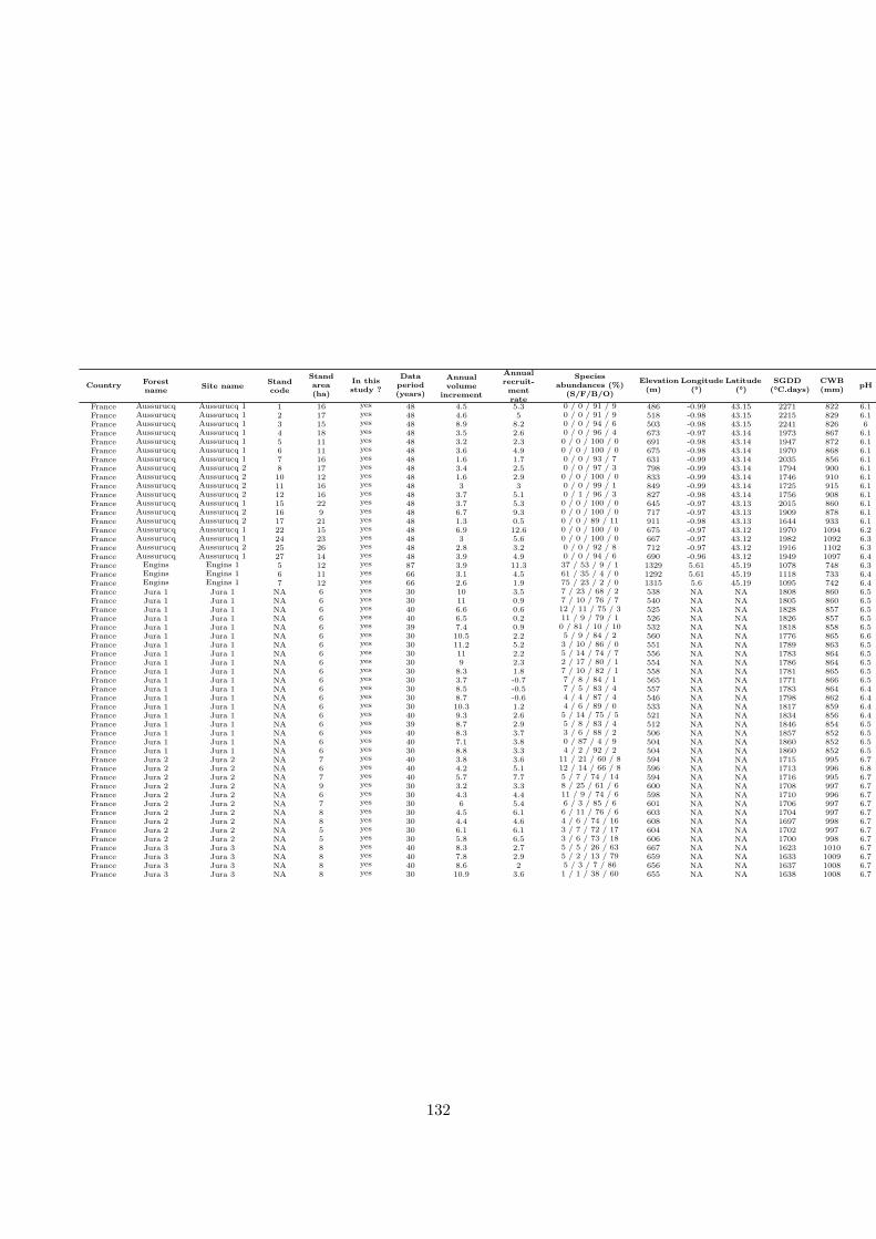
Country Forestname Site name Stand
code
Standarea(ha)
In thisstudy ?
Dataperiod(years)
Annualvolume
increment
Annualrecruit-
mentrate
Speciesabundances (%)
(S/F/B/O)Elevation
(m)Longitude
(°)Latitude
(°)SGDD
(°C.days)CWB(mm) pH SEAS
(°C)
France Aussurucq Aussurucq 1 1 16 yes 48 4.5 5.3 0 / 0 / 91 / 9 486 -0.99 43.15 2271 822 6.1 4.96France Aussurucq Aussurucq 1 2 17 yes 48 4.6 5 0 / 0 / 91 / 9 518 -0.98 43.15 2215 829 6.1 4.97France Aussurucq Aussurucq 1 3 15 yes 48 8.9 8.2 0 / 0 / 94 / 6 503 -0.98 43.15 2241 826 6 4.97France Aussurucq Aussurucq 1 4 18 yes 48 3.5 2.6 0 / 0 / 96 / 4 673 -0.97 43.14 1973 867 6.1 4.99France Aussurucq Aussurucq 1 5 11 yes 48 3.2 2.3 0 / 0 / 100 / 0 691 -0.98 43.14 1947 872 6.1 4.99France Aussurucq Aussurucq 1 6 11 yes 48 3.6 4.9 0 / 0 / 100 / 0 675 -0.98 43.14 1970 868 6.1 4.99France Aussurucq Aussurucq 1 7 16 yes 48 1.6 1.7 0 / 0 / 93 / 7 631 -0.99 43.14 2035 856 6.1 4.98France Aussurucq Aussurucq 2 8 17 yes 48 3.4 2.5 0 / 0 / 97 / 3 798 -0.99 43.14 1794 900 6.1 5France Aussurucq Aussurucq 2 10 12 yes 48 1.6 2.9 0 / 0 / 100 / 0 833 -0.99 43.14 1746 910 6.1 5.01France Aussurucq Aussurucq 2 11 16 yes 48 3 3 0 / 0 / 99 / 1 849 -0.99 43.14 1725 915 6.1 5.01France Aussurucq Aussurucq 2 12 16 yes 48 3.7 5.1 0 / 1 / 96 / 3 827 -0.98 43.14 1756 908 6.1 5.01France Aussurucq Aussurucq 1 15 22 yes 48 3.7 5.3 0 / 0 / 100 / 0 645 -0.97 43.13 2015 860 6.1 4.99France Aussurucq Aussurucq 2 16 9 yes 48 6.7 9.3 0 / 0 / 100 / 0 717 -0.97 43.13 1909 878 6.1 5France Aussurucq Aussurucq 2 17 21 yes 48 1.3 0.5 0 / 0 / 89 / 11 911 -0.98 43.13 1644 933 6.1 5.02France Aussurucq Aussurucq 1 22 15 yes 48 6.9 12.6 0 / 0 / 100 / 0 675 -0.97 43.12 1970 1094 6.2 4.98France Aussurucq Aussurucq 1 24 23 yes 48 3 5.6 0 / 0 / 100 / 0 667 -0.97 43.12 1982 1092 6.3 4.99France Aussurucq Aussurucq 2 25 26 yes 48 2.8 3.2 0 / 0 / 92 / 8 712 -0.97 43.12 1916 1102 6.3 4.99France Aussurucq Aussurucq 1 27 14 yes 48 3.9 4.9 0 / 0 / 94 / 6 690 -0.96 43.12 1949 1097 6.4 4.99France Engins Engins 1 5 12 yes 87 3.9 11.3 37 / 53 / 9 / 1 1329 5.61 45.19 1078 748 6.3 6.17France Engins Engins 1 6 11 yes 66 3.1 4.5 61 / 35 / 4 / 0 1292 5.61 45.19 1118 733 6.4 6.19France Engins Engins 1 7 12 yes 66 2.6 1.9 75 / 23 / 2 / 0 1315 5.6 45.19 1095 742 6.4 6.18France Jura 1 Jura 1 NA 6 yes 30 10 3.5 7 / 23 / 68 / 2 538 NA NA 1808 860 6.5 6.36France Jura 1 Jura 1 NA 6 yes 30 11 0.9 7 / 10 / 76 / 7 540 NA NA 1805 860 6.5 6.36France Jura 1 Jura 1 NA 6 yes 40 6.6 0.6 12 / 11 / 75 / 3 525 NA NA 1828 857 6.5 6.37France Jura 1 Jura 1 NA 6 yes 40 6.5 0.2 11 / 9 / 79 / 1 526 NA NA 1826 857 6.5 6.37France Jura 1 Jura 1 NA 6 yes 39 7.4 0.9 0 / 81 / 10 / 10 532 NA NA 1818 858 6.5 6.37France Jura 1 Jura 1 NA 6 yes 30 10.5 2.2 5 / 9 / 84 / 2 560 NA NA 1776 865 6.6 6.35France Jura 1 Jura 1 NA 6 yes 30 11.2 5.2 3 / 10 / 86 / 0 551 NA NA 1789 863 6.5 6.36France Jura 1 Jura 1 NA 6 yes 30 11 2.2 5 / 14 / 74 / 7 556 NA NA 1783 864 6.5 6.36France Jura 1 Jura 1 NA 6 yes 30 9 2.3 2 / 17 / 80 / 1 554 NA NA 1786 864 6.5 6.36France Jura 1 Jura 1 NA 6 yes 30 8.3 1.8 7 / 10 / 82 / 1 558 NA NA 1781 865 6.5 6.36France Jura 1 Jura 1 NA 6 yes 30 3.7 -0.7 7 / 8 / 84 / 1 565 NA NA 1771 866 6.5 6.35France Jura 1 Jura 1 NA 6 yes 30 8.5 -0.5 7 / 5 / 83 / 4 557 NA NA 1783 864 6.4 6.36France Jura 1 Jura 1 NA 6 yes 30 8.7 -0.6 4 / 4 / 87 / 4 546 NA NA 1798 862 6.4 6.36France Jura 1 Jura 1 NA 6 yes 30 10.3 1.2 4 / 6 / 89 / 0 533 NA NA 1817 859 6.4 6.37France Jura 1 Jura 1 NA 6 yes 40 9.3 2.6 5 / 14 / 75 / 5 521 NA NA 1834 856 6.4 6.37France Jura 1 Jura 1 NA 6 yes 39 8.7 2.9 5 / 8 / 83 / 4 512 NA NA 1846 854 6.5 6.38France Jura 1 Jura 1 NA 6 yes 40 8.3 3.7 3 / 6 / 88 / 2 506 NA NA 1857 852 6.5 6.38France Jura 1 Jura 1 NA 6 yes 40 7.1 3.8 0 / 87 / 4 / 9 504 NA NA 1860 852 6.5 6.38France Jura 1 Jura 1 NA 6 yes 30 8.8 3.3 4 / 2 / 92 / 2 504 NA NA 1860 852 6.5 6.38France Jura 2 Jura 2 NA 7 yes 40 3.8 3.6 11 / 21 / 60 / 8 594 NA NA 1715 995 6.7 6.31France Jura 2 Jura 2 NA 6 yes 40 4.2 5.1 12 / 14 / 66 / 8 596 NA NA 1713 996 6.8 6.31France Jura 2 Jura 2 NA 7 yes 40 5.7 7.7 5 / 7 / 74 / 14 594 NA NA 1716 995 6.7 6.31France Jura 2 Jura 2 NA 9 yes 30 3.2 3.3 8 / 25 / 61 / 6 600 NA NA 1708 997 6.7 6.31France Jura 2 Jura 2 NA 6 yes 30 4.3 4.4 11 / 9 / 74 / 6 598 NA NA 1710 996 6.7 6.31France Jura 2 Jura 2 NA 7 yes 30 6 5.4 6 / 3 / 85 / 6 601 NA NA 1706 997 6.7 6.3France Jura 2 Jura 2 NA 8 yes 30 4.5 6.1 6 / 11 / 76 / 6 603 NA NA 1704 997 6.7 6.3France Jura 2 Jura 2 NA 8 yes 30 4.4 4.6 4 / 6 / 74 / 16 608 NA NA 1697 998 6.7 6.3France Jura 2 Jura 2 NA 5 yes 30 6.1 6.1 3 / 7 / 72 / 17 604 NA NA 1702 997 6.7 6.3France Jura 2 Jura 2 NA 5 yes 30 5.8 6.5 3 / 6 / 73 / 18 606 NA NA 1700 998 6.7 6.3France Jura 3 Jura 3 NA 8 yes 40 8.3 2.7 5 / 5 / 26 / 63 667 NA NA 1623 1010 6.7 6.27France Jura 3 Jura 3 NA 8 yes 40 7.8 2.9 5 / 2 / 13 / 79 659 NA NA 1633 1009 6.7 6.28France Jura 3 Jura 3 NA 8 yes 40 8.6 2 5 / 3 / 7 / 86 656 NA NA 1637 1008 6.7 6.28France Jura 3 Jura 3 NA 8 yes 30 10.9 3.6 1 / 1 / 38 / 60 655 NA NA 1638 1008 6.7 6.28
132
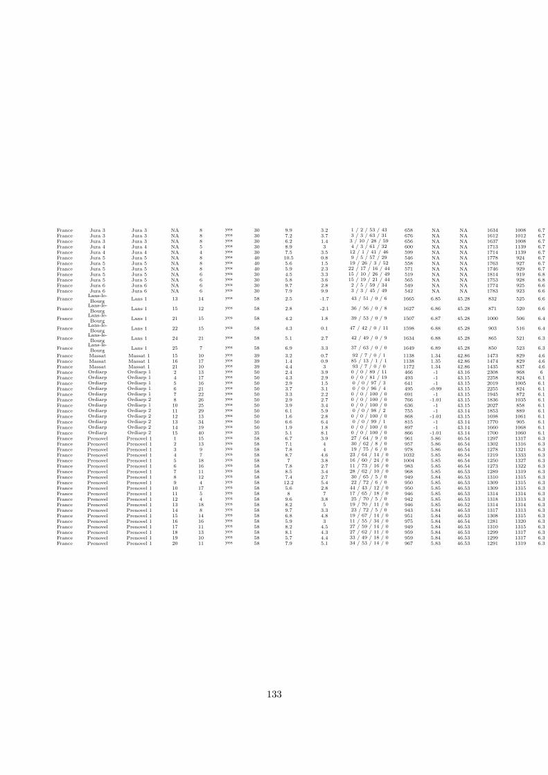
France Jura 3 Jura 3 NA 8 yes 30 9.9 3.2 1 / 2 / 53 / 43 658 NA NA 1634 1008 6.7 6.28France Jura 3 Jura 3 NA 8 yes 30 7.2 3.7 3 / 3 / 63 / 31 676 NA NA 1612 1012 6.7 6.27France Jura 3 Jura 3 NA 8 yes 30 6.2 1.4 3 / 10 / 28 / 59 656 NA NA 1637 1008 6.7 6.28France Jura 4 Jura 4 NA 5 yes 30 8.9 3 4 / 3 / 61 / 32 600 NA NA 1713 1139 6.7 6.31France Jura 4 Jura 4 NA 4 yes 30 7.5 3.5 12 / 1 / 41 / 46 599 NA NA 1714 1139 6.7 6.31France Jura 5 Jura 5 NA 8 yes 40 10.5 0.8 9 / 5 / 57 / 29 546 NA NA 1778 924 6.7 6.33France Jura 5 Jura 5 NA 8 yes 40 5.6 1.5 19 / 26 / 3 / 52 558 NA NA 1763 927 6.7 6.32France Jura 5 Jura 5 NA 8 yes 40 5.9 2.3 22 / 17 / 16 / 44 571 NA NA 1746 929 6.7 6.32France Jura 5 Jura 5 NA 6 yes 30 4.5 3.3 15 / 10 / 26 / 49 519 NA NA 1814 919 6.8 6.34France Jura 5 Jura 5 NA 6 yes 30 5.8 3.6 15 / 19 / 21 / 44 565 NA NA 1753 928 6.8 6.32France Jura 6 Jura 6 NA 6 yes 30 9.7 2.8 2 / 5 / 59 / 34 549 NA NA 1774 925 6.6 6.33France Jura 6 Jura 6 NA 6 yes 30 7.9 9.9 3 / 3 / 45 / 49 542 NA NA 1783 923 6.6 6.33France Lans-le-
Bourg Lans 1 13 14 yes 58 2.5 -1.7 43 / 51 / 0 / 6 1665 6.85 45.28 832 525 6.6 6.21
France Lans-le-Bourg Lans 1 15 12 yes 58 2.8 -2.1 36 / 56 / 0 / 8 1627 6.86 45.28 871 520 6.6 6.24
France Lans-le-Bourg Lans 1 21 15 yes 58 4.2 1.8 39 / 53 / 0 / 9 1507 6.87 45.28 1000 506 6.4 6.34
France Lans-le-Bourg Lans 1 22 15 yes 58 4.3 0.1 47 / 42 / 0 / 11 1598 6.88 45.28 903 516 6.4 6.27
France Lans-le-Bourg Lans 1 24 21 yes 58 5.1 2.7 42 / 49 / 0 / 9 1634 6.88 45.28 865 521 6.3 6.24
France Lans-le-Bourg Lans 1 25 7 yes 58 6.9 3.3 37 / 63 / 0 / 0 1649 6.89 45.28 850 523 6.3 6.23
France Massat Massat 1 15 10 yes 39 3.2 0.7 92 / 7 / 0 / 1 1138 1.34 42.86 1473 829 4.6 5.45France Massat Massat 1 16 17 yes 39 1.4 0.9 85 / 13 / 1 / 1 1138 1.35 42.86 1474 829 4.6 5.45France Massat Massat 1 21 10 yes 39 4.4 3 93 / 7 / 0 / 0 1172 1.34 42.86 1435 837 4.6 5.45France Ordiarp Ordiarp 1 2 13 yes 50 2.4 3.9 0 / 0 / 89 / 11 466 -1 43.16 2308 968 6 4.95France Ordiarp Ordiarp 1 4 17 yes 50 4.3 2.9 0 / 0 / 81 / 19 493 -1 43.15 2258 824 6.1 4.96France Ordiarp Ordiarp 1 5 16 yes 50 2.9 1.5 0 / 0 / 97 / 3 641 -1 43.15 2019 1005 6.1 4.97France Ordiarp Ordiarp 1 6 21 yes 50 3.7 3.1 0 / 0 / 96 / 4 495 -0.99 43.15 2255 824 6.1 4.96France Ordiarp Ordiarp 1 7 22 yes 50 3.3 2.2 0 / 0 / 100 / 0 691 -1 43.15 1945 872 6.1 4.98France Ordiarp Ordiarp 2 8 26 yes 50 2.9 2.7 0 / 0 / 100 / 0 766 -1.01 43.15 1836 1035 6.1 4.99France Ordiarp Ordiarp 1 10 25 yes 50 3.9 3.4 0 / 0 / 100 / 0 636 -1 43.15 2027 858 6.1 4.98France Ordiarp Ordiarp 2 11 29 yes 50 6.1 5.9 0 / 0 / 98 / 2 755 -1 43.14 1853 889 6.1 4.99France Ordiarp Ordiarp 2 12 13 yes 50 1.6 2.8 0 / 0 / 100 / 0 868 -1.01 43.15 1698 1061 6.1 5.01France Ordiarp Ordiarp 2 13 34 yes 50 6.6 6.4 0 / 0 / 99 / 1 815 -1 43.14 1770 905 6.1 5France Ordiarp Ordiarp 2 14 19 yes 50 1.9 1.8 0 / 0 / 100 / 0 897 -1 43.14 1660 1068 6.1 5.01France Ordiarp Ordiarp 2 15 40 yes 35 5.1 8.1 0 / 0 / 100 / 0 866 -1.01 43.14 1700 1060 6.1 5.01France Prenovel Prenovel 1 1 15 yes 58 6.7 3.9 27 / 64 / 9 / 0 961 5.86 46.54 1297 1317 6.3 6.15France Prenovel Prenovel 1 2 13 yes 58 7.1 4 30 / 62 / 8 / 0 957 5.86 46.54 1302 1316 6.3 6.15France Prenovel Prenovel 1 3 9 yes 58 7.8 4 19 / 75 / 6 / 0 978 5.86 46.54 1278 1321 6.3 6.14France Prenovel Prenovel 1 4 7 yes 58 8.7 4.6 23 / 64 / 14 / 0 1032 5.85 46.54 1219 1333 6.3 6.11France Prenovel Prenovel 1 5 18 yes 58 7 3.8 16 / 60 / 24 / 0 1004 5.85 46.54 1250 1327 6.3 6.12France Prenovel Prenovel 1 6 16 yes 58 7.8 2.7 11 / 73 / 16 / 0 983 5.85 46.54 1273 1322 6.3 6.14France Prenovel Prenovel 1 7 11 yes 58 8.5 3.4 28 / 62 / 10 / 0 968 5.85 46.53 1289 1319 6.3 6.14France Prenovel Prenovel 1 8 12 yes 58 7.4 2.7 30 / 65 / 5 / 0 949 5.84 46.53 1310 1315 6.3 6.15France Prenovel Prenovel 1 9 4 yes 58 12.2 5.4 22 / 72 / 6 / 0 950 5.85 46.53 1309 1315 6.3 6.15France Prenovel Prenovel 1 10 17 yes 58 5.6 2.8 44 / 43 / 12 / 0 950 5.85 46.53 1309 1315 6.3 6.15France Prenovel Prenovel 1 11 5 yes 58 8 7 17 / 65 / 18 / 0 946 5.85 46.53 1314 1314 6.3 6.16France Prenovel Prenovel 1 12 4 yes 58 9.6 3.8 25 / 70 / 5 / 0 942 5.85 46.53 1318 1313 6.3 6.16France Prenovel Prenovel 1 13 18 yes 58 8.2 5 19 / 70 / 11 / 0 946 5.85 46.52 1314 1314 6.3 6.16France Prenovel Prenovel 1 14 8 yes 58 9.7 3.3 23 / 72 / 5 / 0 943 5.84 46.53 1317 1313 6.3 6.16France Prenovel Prenovel 1 15 14 yes 58 6.8 4.8 19 / 67 / 14 / 0 951 5.84 46.53 1308 1315 6.3 6.15France Prenovel Prenovel 1 16 16 yes 58 5.9 3 11 / 55 / 34 / 0 975 5.84 46.54 1281 1320 6.3 6.14France Prenovel Prenovel 1 17 11 yes 58 8.2 4.5 27 / 59 / 14 / 0 949 5.84 46.53 1310 1315 6.3 6.15France Prenovel Prenovel 1 18 13 yes 58 8.1 4.3 27 / 62 / 11 / 0 959 5.84 46.53 1299 1317 6.3 6.15France Prenovel Prenovel 1 19 10 yes 58 5.7 4.4 33 / 49 / 18 / 0 959 5.84 46.53 1299 1317 6.3 6.15France Prenovel Prenovel 1 20 11 yes 58 7.9 5.1 34 / 53 / 14 / 0 967 5.83 46.53 1291 1319 6.3 6.15
133
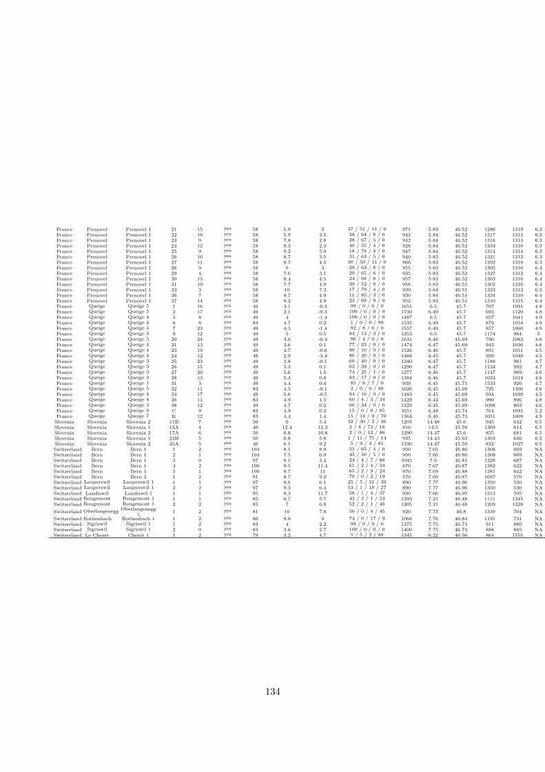
France Prenovel Prenovel 1 21 15 yes 58 5.8 3 37 / 51 / 11 / 0 971 5.83 46.52 1286 1319 6.3 6.14France Prenovel Prenovel 1 22 16 yes 58 5.9 3.5 28 / 64 / 8 / 0 943 5.84 46.52 1317 1313 6.3 6.16France Prenovel Prenovel 1 23 9 yes 58 7.8 2.8 28 / 67 / 5 / 0 942 5.84 46.52 1318 1313 6.3 6.16France Prenovel Prenovel 1 24 12 yes 58 8.3 2.3 40 / 55 / 4 / 0 928 5.84 46.52 1334 1310 6.3 6.17France Prenovel Prenovel 1 25 9 yes 58 9.2 5.9 18 / 78 / 4 / 0 947 5.84 46.52 1314 1314 6.3 6.16France Prenovel Prenovel 1 26 16 yes 58 8.7 3.5 31 / 63 / 5 / 0 940 5.83 46.52 1321 1313 6.3 6.16France Prenovel Prenovel 1 27 11 yes 58 8.7 4.5 30 / 59 / 11 / 0 966 5.83 46.52 1292 1318 6.3 6.15France Prenovel Prenovel 1 28 9 yes 58 6 3 29 / 63 / 8 / 0 955 5.83 46.52 1305 1316 6.4 6.15France Prenovel Prenovel 1 29 4 yes 58 7.6 3.1 29 / 65 / 6 / 0 935 5.83 46.52 1327 1312 6.4 6.16France Prenovel Prenovel 1 30 13 yes 58 8.4 4.5 24 / 68 / 8 / 0 957 5.83 46.52 1303 1316 6.4 6.15France Prenovel Prenovel 1 31 10 yes 58 7.7 4.9 39 / 52 / 9 / 0 958 5.83 46.51 1302 1316 6.4 6.15France Prenovel Prenovel 1 33 3 yes 58 10 7.3 17 / 79 / 4 / 0 939 5.84 46.51 1323 1312 6.3 6.16France Prenovel Prenovel 1 36 7 yes 58 8.7 4.9 11 / 85 / 3 / 0 930 5.84 46.51 1334 1310 6.4 6.17France Prenovel Prenovel 1 37 14 yes 58 8.2 4.8 23 / 69 / 9 / 0 952 5.83 46.51 1310 1315 6.4 6.16France Queige Queige 5 1 16 yes 49 3.1 -0.3 99 / 0 / 0 / 0 1651 6.5 45.7 767 1091 4.8 6.03France Queige Queige 5 2 17 yes 49 2.1 -0.3 100 / 0 / 0 / 0 1730 6.49 45.7 693 1120 4.8 5.98France Queige Queige 4 5 8 yes 49 4 -1.4 100 / 0 / 0 / 0 1487 6.5 45.7 927 1041 4.9 6.14France Queige Queige 4 6 8 yes 83 4.7 0.2 1 / 0 / 0 / 99 1535 6.49 45.7 879 1054 4.9 6.11France Queige Queige 4 7 23 yes 49 4.3 -1.4 92 / 8 / 0 / 0 1557 6.49 45.7 857 1060 4.9 6.09France Queige Queige 3 9 12 yes 49 5 0.5 84 / 13 / 3 / 0 1253 6.5 45.7 1174 984 5 6.3France Queige Queige 5 20 24 yes 49 3.6 -0.4 96 / 4 / 0 / 0 1631 6.46 45.69 790 1083 4.6 6.05France Queige Queige 4 21 13 yes 49 3.6 0.1 77 / 23 / 0 / 0 1474 6.47 45.69 943 1036 4.6 6.15France Queige Queige 4 23 19 yes 49 4.7 -0.6 90 / 10 / 0 / 0 1526 6.46 45.7 891 1051 4.5 6.11France Queige Queige 4 24 12 yes 49 2.9 -3.4 80 / 20 / 0 / 0 1488 6.45 45.7 929 1040 4.5 6.14France Queige Queige 3 25 23 yes 49 3.8 -0.1 60 / 40 / 0 / 0 1240 6.47 45.7 1188 981 4.7 6.3France Queige Queige 3 26 15 yes 49 5.3 0.1 62 / 38 / 0 / 0 1290 6.47 45.7 1134 992 4.7 6.27France Queige Queige 3 27 20 yes 49 5.6 1.5 74 / 25 / 1 / 0 1277 6.46 45.7 1147 989 4.6 6.28France Queige Queige 3 28 13 yes 49 5.3 0.8 83 / 17 / 0 / 0 1384 6.46 45.7 1034 1014 4.6 6.21France Queige Queige 1 31 3 yes 49 4.4 0.4 85 / 8 / 7 / 0 939 6.45 45.71 1533 926 4.7 6.51France Queige Queige 5 32 11 yes 83 4.5 -0.1 2 / 0 / 0 / 98 1626 6.45 45.69 795 1306 4.6 6.05France Queige Queige 4 34 17 yes 49 5.6 -0.5 84 / 16 / 0 / 0 1483 6.45 45.69 934 1039 4.5 6.14France Queige Queige 4 36 11 yes 83 4.9 1.5 60 / 4 / 3 / 34 1429 6.44 45.69 990 896 4.8 6.18France Queige Queige 3 38 12 yes 49 4.7 0.2 66 / 34 / 0 / 0 1323 6.45 45.69 1098 863 4.6 6.25France Queige Queige 9 C 9 yes 83 3.9 0.3 15 / 0 / 0 / 85 1651 6.48 45.74 764 1091 5.2 6.03France Queige Queige 7 K 12 yes 83 4.4 1.4 15 / 14 / 0 / 70 1364 6.46 45.73 1051 1009 4.9 6.22
Slovenia Slovenia Slovenia 2 11B 7 yes 50 6 5.4 32 / 30 / 2 / 36 1205 14.48 45.6 945 642 6.5 6.22Slovenia Slovenia Slovenia 1 13A 4 yes 40 12.4 12.3 2 / 8 / 72 / 18 810 14.5 45.59 1369 614 6.5 6.44Slovenia Slovenia Slovenia 2 17A 6 yes 50 6.8 16.8 2 / 0 / 12 / 86 1290 14.47 45.6 855 681 6.5 6.14Slovenia Slovenia Slovenia 1 23H 5 yes 50 6.8 5.8 1 / 11 / 75 / 14 935 14.43 45.63 1304 646 6.5 6.55Slovenia Slovenia Slovenia 2 45A 5 yes 40 6.1 9.2 5 / 9 / 4 / 81 1330 14.47 45.59 832 1027 6.5 6.18Switzerland Bern Bern 1 1 2 yes 104 8.1 8.9 31 / 65 / 4 / 0 950 7.65 46.86 1308 669 NA 6.18Switzerland Bern Bern 1 2 1 yes 104 7.5 6.9 45 / 50 / 5 / 0 950 7.66 46.86 1308 669 NA 6.18Switzerland Bern Bern 1 3 0 yes 97 6.1 3.4 24 / 4 / 7 / 66 1045 7.6 46.81 1228 687 NA 6.15Switzerland Bern Bern 1 4 2 yes 100 8.5 11.4 61 / 2 / 4 / 34 870 7.67 46.87 1382 622 NA 6.22Switzerland Bern Bern 1 5 1 yes 100 8.7 11 65 / 2 / 9 / 24 970 7.69 46.88 1281 642 NA 6.15Switzerland Bern Bern 2 1 2 yes 91 8.7 9.2 79 / 0 / 2 / 19 570 7.69 46.87 1697 570 NA 6.43Switzerland Lauperswil Lauperswil 1 1 1 yes 97 8.6 6.1 25 / 5 / 31 / 39 890 7.77 46.96 1350 530 NA 6.17Switzerland Lauperswil Lauperswil 1 2 2 yes 97 9.3 6.4 53 / 1 / 18 / 27 890 7.77 46.96 1350 530 NA 6.17Switzerland Landiswil Landiswil 1 1 1 yes 95 8.3 11.7 58 / 1 / 4 / 37 930 7.66 46.95 1313 595 NA 6.14Switzerland Rougemont Rougemont 1 1 1 yes 85 6.7 5.7 43 / 3 / 1 / 53 1293 7.21 46.48 1111 1345 NA 6.23Switzerland Rougemont Rougemont 1 2 2 yes 85 7 6.9 52 / 2 / 1 / 46 1205 7.21 46.48 1209 1328 NA 6.29Switzerland Oberlangenegg Oberlangenegg
1 1 2 yes 81 10 7.8 50 / 0 / 4 / 45 920 7.73 46.8 1339 704 NA 6.19Switzerland Rothenbach Rothenbach 1 1 2 yes 80 8.8 9 74 / 0 / 17 / 9 1068 7.76 46.84 1191 731 NA 6.1Switzerland Sigriswil Sigriswil 1 1 2 yes 83 4 2.2 99 / 0 / 0 / 0 1375 7.75 46.73 911 880 NA 5.96Switzerland Sigriswil Sigriswil 1 2 0 yes 83 3.6 2.7 100 / 0 / 0 / 0 1400 7.75 46.73 888 885 NA 5.95Switzerland Le Chenit Chenit 1 1 2 yes 79 3.2 4.7 5 / 5 / 2 / 88 1345 6.22 46.56 864 1555 NA 5.88
134

Table A.1: Data summary. Each line is a stand. Data period is the mean time between the oldest and the youngest inventories. The annual volumeincrement values are speciied in m3.ha−1.year−1, the annual recruitment rate in nb.ha−1.year−1. The abbreviations S, F, B and O for the species
abundances mean respectively Spruce, Fir, Beech and Other species; the abundances are given in % of the total basal area. SGDD = annual Sum ofGrowing Degree-Days; CWB = Climatic Water Budget (see the main text for computation details).
135

Site deinition
Basically, the sites corresponded to forests, except for the large forests encompassing a large altitudinalgradient, which were further divided into multiple sites in order to have homogeneous climatic conditionswithin sites. The Queige forest was divided in two sub-forest groups because its stands are located in twoisolated and opposite slopes (43 stands in the North slope and 11 in the South slope), resulting in contrastedenvironmental conditions (not only in terms of thermal conditions) and management regimes.
A clustering technique was then applied to the stands, which was based on the SGDD values computedfor each stand. We used the “kmeans” R function (R Core Team, 2015), which is based on the algorithmdeveloped by Hartigan and Wong (1979). The function was applied on all stands taken together and thechoice of the number of clusters was based on a qualitative trade-of between a low within-site variability ofthermal conditions and a large number of stands by site.
In the end, only 7 forests were split in multiple sites (Aussurucq, Queige - North and South slopes, Lente,Ordiarp, Slovenia and Bern) (Table 1 and B1). For the Queige forest, the clustering algorithm divided theNorth slope in 6 sites and the South slope in 3 sites. The four other forests were divided only in two siteseach.
136

B. Temperature correction in function of elevation
For each stand, the monthly temperatures were extracted from temperature raster layers (from the World-Clim data for the Slovenian stands, and from the SAFRAN data for the French and Swiss stands). Giventhat the study stands were located in mountain ranges, that temperature is closely related to elevation andthat the meteorological data were of a too coarse spatial resolution, we corrected the temperature data ex-tracted from the raster layers according to the stand elevations, adapting the interpolation technique used byKunstler et al. (2011)). First, the closest neighbor raster cell (the “reference” cell) to the stand location wasselected. Then, all raster cells which were located 25km around the reference cell were considered to estimatethe linear relation between temperature and elevation. The stand temperature was inally computed usingthe result of this linear regression. This procedure was applied for each stand and each month independently.
137
C. Speciic recalibration features for this study
Basically, the recalibration method used in the present study reproduced the method presented by Lagar-rigues et al. (2015), hereafter referenced as previous study. However, several technical points were improvedand/or adapted to the present study.
Data pre-treatment
The management data collected for this study came from diferent sources. As a result, the informationavailable in the data was heterogeneous. We therefore compiled the following minimal set of always availablepieces of information:
• Only the trees whose dbh was greater than 17.5 cm were considered in the forest inventories.• All harvestings were grouped (ordinary cuts, salvage cuts, cuts for forest road construction, …).• Only the quantity and the volume of harvested trees were considered.• The harvestings were grouped in 20 years-long periods.
There was an exception for of the Aussurucq and Ordiarp forests : the last inventories gave only statisticalinformation about the density (basal area) of trees in 4 dbh categories.
Recalibrated parameters
The recalibrated growth parameter in the present study was the same than that of the previous study. On thecontrary, we recalibrated a regeneration parameter independent of adult density in the present study to takeinto account the signiicant shifts of species composition in several stands, which could not have been modeledwith a density-dependent regeneration such as the one performed in the previous study. Complementaryinformation about the regeneration process in Samsara2 can be found in the main text of this study and inthe material and methods presented in Lagarrigues et al. (2015) and Courbaud et al. (2015).
Initialization of the sapling layer
Initial sapling composition, abundance and locations were simulated using Samsara2 regeneration process:a 100-year long demographical dynamics was simulated, applying only the sapling installation and saplinggrowth processes with no change in the adult stand. Saplings reaching the recruitment height thresholdduring that phase were not recruited as adult trees but simply removed. Adult trees (dbh > 7.5, 10 or 17.5cm for Swiss, Slovenian and French forests respectively) were thus not impacted by this initialization step.We found that 100 years were suicient to obtain a quasi-equilibrium between sapling installation (inputs)and recruitment (outputs) and thus a sapling population in balance with the adult stand. It is noteworthythat this initialization step depends on the calibrated Samsara2 regeneration parameter and therefore thatthis step was calibrated together with the dynamic phase (reproduction of the stand historic).
ABC procedure
Summary statistics
The summary statistics were computed on adult trees only. The minimum diameter at breast height (DBH)to consider a tree as an adult was 20 cm for the Slovenian stands (where the diameter classes used in inventorydata are deined in the format 20-25 cm) and 17.5 cm for others (where the diameter classes are deined inthe format 17.5-22.5 cm). Unlike in the previous study, as the distributions by diameter classes were notavailable for all data, we only used the quantity and the volume of adult trees as summary statistics for thepresent study (and only the volume for the Aussurucq and Ordiarp stands).
138

Number of simulations
Although 20,000 simulations were found to be necessary in the previous study, we carried out 10,000 simu-lations in the present study for each stand. The new summary statistics used here enabled this increasedconvergence speed. Besides, we checked the convergence of the posterior distributions, which was valid forall stands with 10,000 simulations. The acceptance rate was chosen in accordance with the previous study(0.05), which resulted in 500 accepted simulations for each stand.
Transformation of data
The posterior distributions were restricted in the prior ranges using the transformation technique providedby the “abc” R package (logit transformation).
139
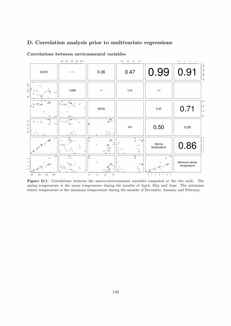
D. Correlation analysis prior to multivariate regressions
Correlations between environmental variables
SGDD
600 800 1000 1200 1400
0.13 0.36
5.0 5.5 6.0 6.5
0.47 0.99
−2 0 2 4
800
1200
1600
2000
0.91
600
1000
1400
CWB 0.13 0.22 0.16 0.041
SEAS 0.067 0.25
5.0
5.5
6.0
6.5
0.71
5.0
5.5
6.0
6.5
pH 0.50 0.29
Springtemperature
34
56
78
9
0.86
800 1200 1600 2000
−2
02
4
5.0 5.5 6.0 6.5 3 4 5 6 7 8 9
Minimum wintertemperature
Figure D.1: Correlations between the macro-environmental variables computed at the site scale. Thespring temperature is the mean temperature during the months of April, May and June. The minimumwinter temperature is the minimum temperature during the months of December, January and February.
140

Species Process Mean date Period lengthSpruce Growth 0.11 0.07Spruce Regeneration -0.13 0.24Fir Growth 0.3 -0.09Fir Regeneration 0.24 -0.04
Beech Growth 0.1 0.06Beech Regeneration -0.22 0.19
Table D.1: The process identiies the demographic variable considered : Growth stands for GA parameter,Regeneration for RA parameter. Correlations were computed between these demographic variables andthe mean inventory dates (= (youngest + oldest inventory dates)/2) (column Mean date) and betweendemographic variables and period lengths (=youngest - oldest inventory dates) (column Period length).
141
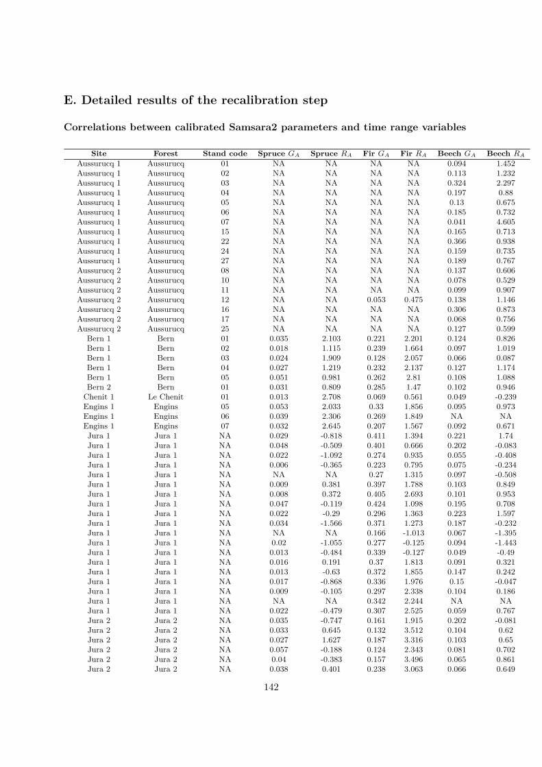
E. Detailed results of the recalibration step
Correlations between calibrated Samsara2 parameters and time range variables
Site Forest Stand code Spruce GA Spruce RA Fir GA Fir RA Beech GA Beech RA
Aussurucq 1 Aussurucq 01 NA NA NA NA 0.094 1.452Aussurucq 1 Aussurucq 02 NA NA NA NA 0.113 1.232Aussurucq 1 Aussurucq 03 NA NA NA NA 0.324 2.297Aussurucq 1 Aussurucq 04 NA NA NA NA 0.197 0.88Aussurucq 1 Aussurucq 05 NA NA NA NA 0.13 0.675Aussurucq 1 Aussurucq 06 NA NA NA NA 0.185 0.732Aussurucq 1 Aussurucq 07 NA NA NA NA 0.041 4.605Aussurucq 1 Aussurucq 15 NA NA NA NA 0.165 0.713Aussurucq 1 Aussurucq 22 NA NA NA NA 0.366 0.938Aussurucq 1 Aussurucq 24 NA NA NA NA 0.159 0.735Aussurucq 1 Aussurucq 27 NA NA NA NA 0.189 0.767Aussurucq 2 Aussurucq 08 NA NA NA NA 0.137 0.606Aussurucq 2 Aussurucq 10 NA NA NA NA 0.078 0.529Aussurucq 2 Aussurucq 11 NA NA NA NA 0.099 0.907Aussurucq 2 Aussurucq 12 NA NA 0.053 0.475 0.138 1.146Aussurucq 2 Aussurucq 16 NA NA NA NA 0.306 0.873Aussurucq 2 Aussurucq 17 NA NA NA NA 0.068 0.756Aussurucq 2 Aussurucq 25 NA NA NA NA 0.127 0.599
Bern 1 Bern 01 0.035 2.103 0.221 2.201 0.124 0.826Bern 1 Bern 02 0.018 1.115 0.239 1.664 0.097 1.019Bern 1 Bern 03 0.024 1.909 0.128 2.057 0.066 0.087Bern 1 Bern 04 0.027 1.219 0.232 2.137 0.127 1.174Bern 1 Bern 05 0.051 0.981 0.262 2.81 0.108 1.088Bern 2 Bern 01 0.031 0.809 0.285 1.47 0.102 0.946
Chenit 1 Le Chenit 01 0.013 2.708 0.069 0.561 0.049 -0.239Engins 1 Engins 05 0.053 2.033 0.33 1.856 0.095 0.973Engins 1 Engins 06 0.039 2.306 0.269 1.849 NA NAEngins 1 Engins 07 0.032 2.645 0.207 1.567 0.092 0.671Jura 1 Jura 1 NA 0.029 -0.818 0.411 1.394 0.221 1.74Jura 1 Jura 1 NA 0.048 -0.509 0.401 0.666 0.202 -0.083Jura 1 Jura 1 NA 0.022 -1.092 0.274 0.935 0.055 -0.408Jura 1 Jura 1 NA 0.006 -0.365 0.223 0.795 0.075 -0.234Jura 1 Jura 1 NA NA NA 0.27 1.315 0.097 -0.508Jura 1 Jura 1 NA 0.009 0.381 0.397 1.788 0.103 0.849Jura 1 Jura 1 NA 0.008 0.372 0.405 2.693 0.101 0.953Jura 1 Jura 1 NA 0.047 -0.119 0.424 1.098 0.195 0.708Jura 1 Jura 1 NA 0.022 -0.29 0.296 1.363 0.223 1.597Jura 1 Jura 1 NA 0.034 -1.566 0.371 1.273 0.187 -0.232Jura 1 Jura 1 NA NA NA 0.166 -1.013 0.067 -1.395Jura 1 Jura 1 NA 0.02 -1.055 0.277 -0.125 0.094 -1.443Jura 1 Jura 1 NA 0.013 -0.484 0.339 -0.127 0.049 -0.49Jura 1 Jura 1 NA 0.016 0.191 0.37 1.813 0.091 0.321Jura 1 Jura 1 NA 0.013 -0.63 0.372 1.855 0.147 0.242Jura 1 Jura 1 NA 0.017 -0.868 0.336 1.976 0.15 -0.047Jura 1 Jura 1 NA 0.009 -0.105 0.297 2.338 0.104 0.186Jura 1 Jura 1 NA NA NA 0.342 2.244 NA NAJura 1 Jura 1 NA 0.022 -0.479 0.307 2.525 0.059 0.767Jura 2 Jura 2 NA 0.035 -0.747 0.161 1.915 0.202 -0.081Jura 2 Jura 2 NA 0.033 0.645 0.132 3.512 0.104 0.62Jura 2 Jura 2 NA 0.027 1.627 0.187 3.316 0.103 0.65Jura 2 Jura 2 NA 0.057 -0.188 0.124 2.343 0.081 0.702Jura 2 Jura 2 NA 0.04 -0.383 0.157 3.496 0.065 0.861Jura 2 Jura 2 NA 0.038 0.401 0.238 3.063 0.066 0.649
142
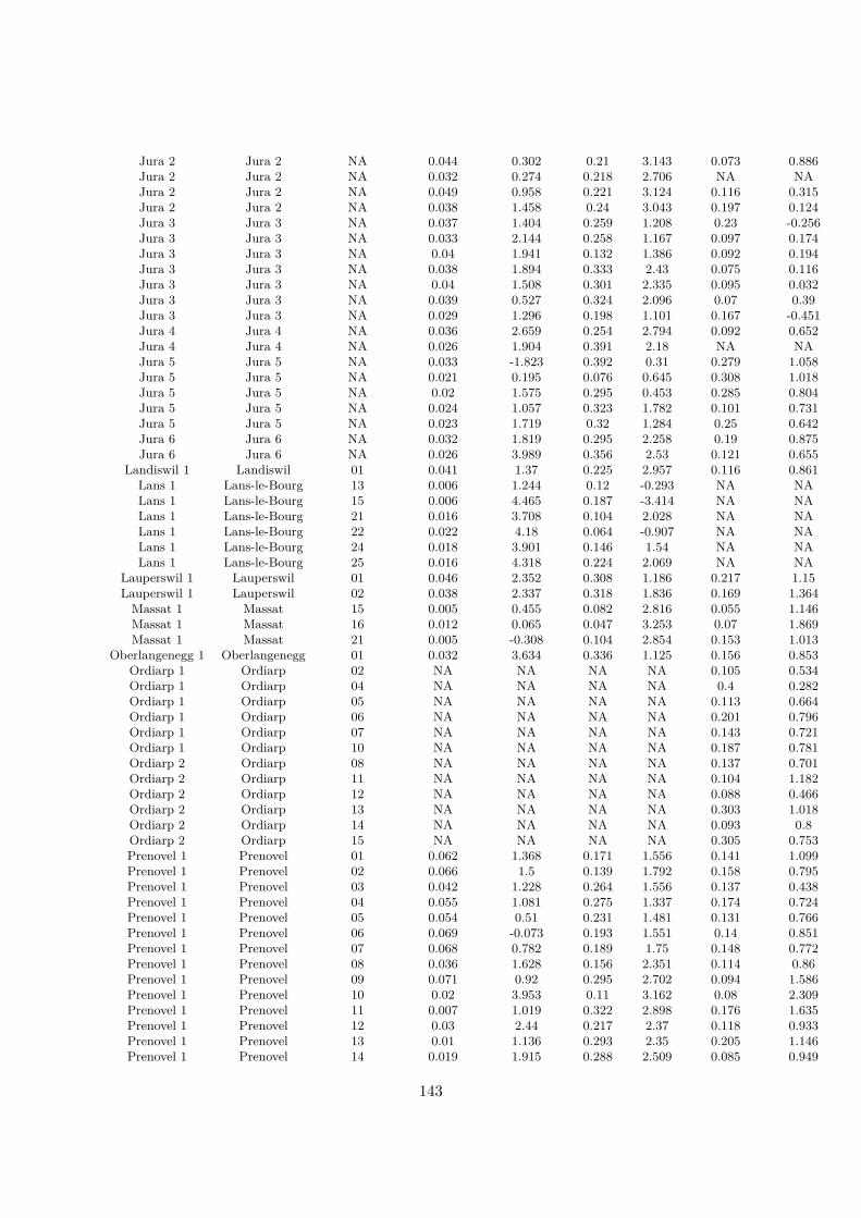
Jura 2 Jura 2 NA 0.044 0.302 0.21 3.143 0.073 0.886Jura 2 Jura 2 NA 0.032 0.274 0.218 2.706 NA NAJura 2 Jura 2 NA 0.049 0.958 0.221 3.124 0.116 0.315Jura 2 Jura 2 NA 0.038 1.458 0.24 3.043 0.197 0.124Jura 3 Jura 3 NA 0.037 1.404 0.259 1.208 0.23 -0.256Jura 3 Jura 3 NA 0.033 2.144 0.258 1.167 0.097 0.174Jura 3 Jura 3 NA 0.04 1.941 0.132 1.386 0.092 0.194Jura 3 Jura 3 NA 0.038 1.894 0.333 2.43 0.075 0.116Jura 3 Jura 3 NA 0.04 1.508 0.301 2.335 0.095 0.032Jura 3 Jura 3 NA 0.039 0.527 0.324 2.096 0.07 0.39Jura 3 Jura 3 NA 0.029 1.296 0.198 1.101 0.167 -0.451Jura 4 Jura 4 NA 0.036 2.659 0.254 2.794 0.092 0.652Jura 4 Jura 4 NA 0.026 1.904 0.391 2.18 NA NAJura 5 Jura 5 NA 0.033 -1.823 0.392 0.31 0.279 1.058Jura 5 Jura 5 NA 0.021 0.195 0.076 0.645 0.308 1.018Jura 5 Jura 5 NA 0.02 1.575 0.295 0.453 0.285 0.804Jura 5 Jura 5 NA 0.024 1.057 0.323 1.782 0.101 0.731Jura 5 Jura 5 NA 0.023 1.719 0.32 1.284 0.25 0.642Jura 6 Jura 6 NA 0.032 1.819 0.295 2.258 0.19 0.875Jura 6 Jura 6 NA 0.026 3.989 0.356 2.53 0.121 0.655
Landiswil 1 Landiswil 01 0.041 1.37 0.225 2.957 0.116 0.861Lans 1 Lans-le-Bourg 13 0.006 1.244 0.12 -0.293 NA NALans 1 Lans-le-Bourg 15 0.006 4.465 0.187 -3.414 NA NALans 1 Lans-le-Bourg 21 0.016 3.708 0.104 2.028 NA NALans 1 Lans-le-Bourg 22 0.022 4.18 0.064 -0.907 NA NALans 1 Lans-le-Bourg 24 0.018 3.901 0.146 1.54 NA NALans 1 Lans-le-Bourg 25 0.016 4.318 0.224 2.069 NA NA
Lauperswil 1 Lauperswil 01 0.046 2.352 0.308 1.186 0.217 1.15Lauperswil 1 Lauperswil 02 0.038 2.337 0.318 1.836 0.169 1.364
Massat 1 Massat 15 0.005 0.455 0.082 2.816 0.055 1.146Massat 1 Massat 16 0.012 0.065 0.047 3.253 0.07 1.869Massat 1 Massat 21 0.005 -0.308 0.104 2.854 0.153 1.013
Oberlangenegg 1 Oberlangenegg 01 0.032 3.634 0.336 1.125 0.156 0.853Ordiarp 1 Ordiarp 02 NA NA NA NA 0.105 0.534Ordiarp 1 Ordiarp 04 NA NA NA NA 0.4 0.282Ordiarp 1 Ordiarp 05 NA NA NA NA 0.113 0.664Ordiarp 1 Ordiarp 06 NA NA NA NA 0.201 0.796Ordiarp 1 Ordiarp 07 NA NA NA NA 0.143 0.721Ordiarp 1 Ordiarp 10 NA NA NA NA 0.187 0.781Ordiarp 2 Ordiarp 08 NA NA NA NA 0.137 0.701Ordiarp 2 Ordiarp 11 NA NA NA NA 0.104 1.182Ordiarp 2 Ordiarp 12 NA NA NA NA 0.088 0.466Ordiarp 2 Ordiarp 13 NA NA NA NA 0.303 1.018Ordiarp 2 Ordiarp 14 NA NA NA NA 0.093 0.8Ordiarp 2 Ordiarp 15 NA NA NA NA 0.305 0.753Prenovel 1 Prenovel 01 0.062 1.368 0.171 1.556 0.141 1.099Prenovel 1 Prenovel 02 0.066 1.5 0.139 1.792 0.158 0.795Prenovel 1 Prenovel 03 0.042 1.228 0.264 1.556 0.137 0.438Prenovel 1 Prenovel 04 0.055 1.081 0.275 1.337 0.174 0.724Prenovel 1 Prenovel 05 0.054 0.51 0.231 1.481 0.131 0.766Prenovel 1 Prenovel 06 0.069 -0.073 0.193 1.551 0.14 0.851Prenovel 1 Prenovel 07 0.068 0.782 0.189 1.75 0.148 0.772Prenovel 1 Prenovel 08 0.036 1.628 0.156 2.351 0.114 0.86Prenovel 1 Prenovel 09 0.071 0.92 0.295 2.702 0.094 1.586Prenovel 1 Prenovel 10 0.02 3.953 0.11 3.162 0.08 2.309Prenovel 1 Prenovel 11 0.007 1.019 0.322 2.898 0.176 1.635Prenovel 1 Prenovel 12 0.03 2.44 0.217 2.37 0.118 0.933Prenovel 1 Prenovel 13 0.01 1.136 0.293 2.35 0.205 1.146Prenovel 1 Prenovel 14 0.019 1.915 0.288 2.509 0.085 0.949
143
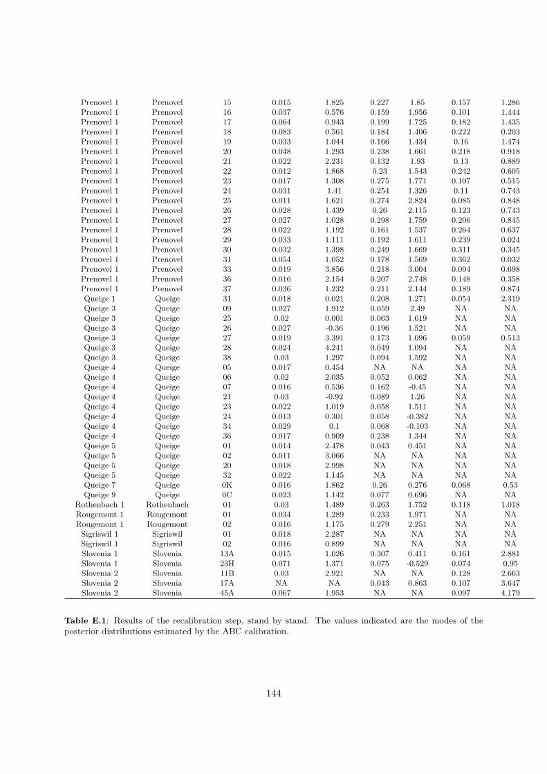
Prenovel 1 Prenovel 15 0.015 1.825 0.227 1.85 0.157 1.286Prenovel 1 Prenovel 16 0.037 0.576 0.159 1.956 0.101 1.444Prenovel 1 Prenovel 17 0.064 0.943 0.199 1.725 0.182 1.435Prenovel 1 Prenovel 18 0.083 0.561 0.184 1.406 0.222 0.203Prenovel 1 Prenovel 19 0.033 1.044 0.166 1.434 0.16 1.474Prenovel 1 Prenovel 20 0.048 1.293 0.238 1.661 0.218 0.918Prenovel 1 Prenovel 21 0.022 2.231 0.132 1.93 0.13 0.889Prenovel 1 Prenovel 22 0.012 1.868 0.23 1.543 0.242 0.605Prenovel 1 Prenovel 23 0.017 1.308 0.275 1.771 0.107 0.515Prenovel 1 Prenovel 24 0.031 1.41 0.254 1.326 0.11 0.743Prenovel 1 Prenovel 25 0.011 1.621 0.274 2.824 0.085 0.848Prenovel 1 Prenovel 26 0.028 1.439 0.26 2.115 0.123 0.743Prenovel 1 Prenovel 27 0.027 1.028 0.298 1.759 0.206 0.845Prenovel 1 Prenovel 28 0.022 1.192 0.161 1.537 0.264 0.637Prenovel 1 Prenovel 29 0.033 1.111 0.192 1.611 0.239 0.024Prenovel 1 Prenovel 30 0.032 1.398 0.249 1.669 0.311 0.345Prenovel 1 Prenovel 31 0.054 1.052 0.178 1.569 0.362 0.032Prenovel 1 Prenovel 33 0.019 3.856 0.218 3.004 0.094 0.698Prenovel 1 Prenovel 36 0.016 2.154 0.207 2.748 0.148 0.358Prenovel 1 Prenovel 37 0.036 1.232 0.211 2.144 0.189 0.874Queige 1 Queige 31 0.018 0.021 0.208 1.271 0.054 2.319Queige 3 Queige 09 0.027 1.912 0.059 2.49 NA NAQueige 3 Queige 25 0.02 0.001 0.063 1.619 NA NAQueige 3 Queige 26 0.027 -0.36 0.196 1.521 NA NAQueige 3 Queige 27 0.019 3.391 0.173 1.096 0.059 0.513Queige 3 Queige 28 0.024 4.241 0.049 1.094 NA NAQueige 3 Queige 38 0.03 1.297 0.094 1.592 NA NAQueige 4 Queige 05 0.017 0.454 NA NA NA NAQueige 4 Queige 06 0.02 2.035 0.052 0.062 NA NAQueige 4 Queige 07 0.016 0.536 0.162 -0.45 NA NAQueige 4 Queige 21 0.03 -0.92 0.089 1.26 NA NAQueige 4 Queige 23 0.022 1.019 0.058 1.511 NA NAQueige 4 Queige 24 0.013 0.301 0.058 -0.382 NA NAQueige 4 Queige 34 0.029 0.1 0.068 -0.103 NA NAQueige 4 Queige 36 0.017 0.909 0.238 1.344 NA NAQueige 5 Queige 01 0.014 2.478 0.043 0.451 NA NAQueige 5 Queige 02 0.011 3.066 NA NA NA NAQueige 5 Queige 20 0.018 2.998 NA NA NA NAQueige 5 Queige 32 0.022 1.145 NA NA NA NAQueige 7 Queige 0K 0.016 1.862 0.26 0.276 0.068 0.53Queige 9 Queige 0C 0.023 1.142 0.077 0.696 NA NA
Rothenbach 1 Rothenbach 01 0.03 1.489 0.263 1.752 0.118 1.018Rougemont 1 Rougemont 01 0.034 1.289 0.233 1.971 NA NARougemont 1 Rougemont 02 0.016 1.175 0.279 2.251 NA NA
Sigriswil 1 Sigriswil 01 0.018 2.287 NA NA NA NASigriswil 1 Sigriswil 02 0.016 0.899 NA NA NA NASlovenia 1 Slovenia 13A 0.015 1.026 0.307 0.411 0.161 2.881Slovenia 1 Slovenia 23H 0.071 1.371 0.075 -0.529 0.074 0.95Slovenia 2 Slovenia 11B 0.03 2.921 NA NA 0.128 2.663Slovenia 2 Slovenia 17A NA NA 0.043 0.863 0.107 3.647Slovenia 2 Slovenia 45A 0.067 1.953 NA NA 0.097 4.179
Table E.1: Results of the recalibration step, stand by stand. The values indicated are the modes of theposterior distributions estimated by the ABC calibration.
144
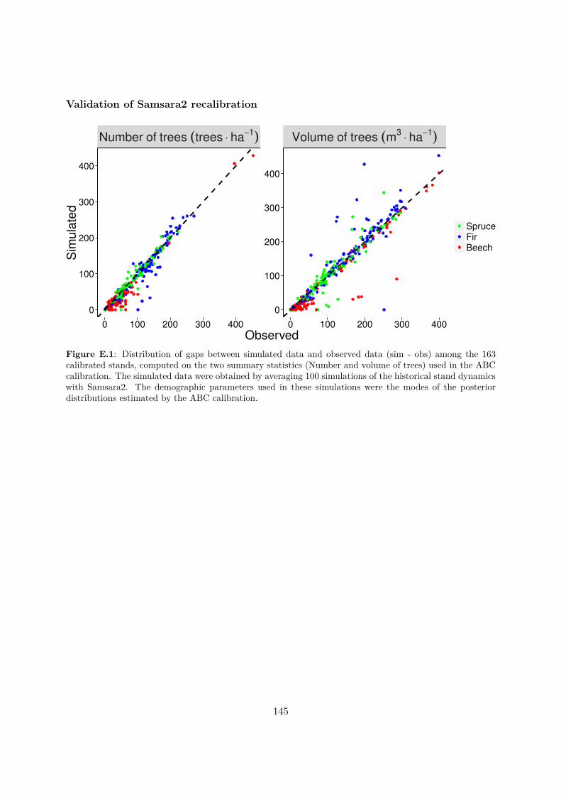
Validation of Samsara2 recalibration
Number of trees (trees ⋅ ha−1) Volume of trees (m3
⋅ ha−1)
0
100
200
300
400
0
100
200
300
400
0 100 200 300 400 0 100 200 300 400
Observed
Sim
ula
ted
SpruceFirBeech
Figure E.1: Distribution of gaps between simulated data and observed data (sim - obs) among the 163calibrated stands, computed on the two summary statistics (Number and volume of trees) used in the ABCcalibration. The simulated data were obtained by averaging 100 simulations of the historical stand dynamicswith Samsara2. The demographic parameters used in these simulations were the modes of the posteriordistributions estimated by the ABC calibration.
145

References
Courbaud, B., Lafond, V., Lagarrigues, G., Vieilledent, G., Cordonnier, T., Jabot, F., De Coligny, F., 2015.Applying ecological model evaludation: Lessons learned with the forest dynamics model Samsara2.Ecological Modelling 314, 1–14.
Hartigan, J.A., Wong, M.A., 1979. Algorithm AS 136: A K-Means Clustering Algorithm. Journal of theRoyal Statistical Society. Series C (Applied Statistics) 28, 100–108. doi:10.2307/2346830
Kunstler, G., Albert, C.H., Courbaud, B., Lavergne, S., Thuiller, W., Vieilledent, G., Zimmermann, N.E.,Coomes, D.A., 2011. Efects of competition on tree radial-growth vary in importance but not in intensityalong climatic gradients. Journal of Ecology 99, 300–312.
Lagarrigues, G., Jabot, F., Lafond, V., Courbaud, B., 2015. Approximate Bayesian computation torecalibrate individual-based models with population data: Illustration with a forest simulation model.Ecological Modelling 306, 278–286.
R Core Team, 2015. R: A Language and Environment for Statistical Computing. R Foundation forStatistical Computing, Vienna, Austria.
146

Annexe C : article asscoié à la partie 4
Article en préparation pour Annals of Forest Science
147

Stand-level management options to preserve goods and services pro-vided by uneven-aged mountain forests in a context of climate change
Guillaume Lagarrigues1*, Franck Jabot2, Sylvain Dupire1, Benoît Courbaud1
1. Université Grenoble Alpes, Irstea, UR EMGR, 2 rue de la Papeterie-BP 76, F-38402 St-Martin-d’Hères,France.
2. LISC-Laboratoire d’Ingénierie pour les Systèmes complexes, IRSTEA, 9 Avenue Blaise Pascal, CS 20085,63178 Aubière, France
*Corresponding author : Guillaume Lagarrigues
Email : [email protected]
Phone number : +33 (0)4 76 76 27 07
Fax number : +33 (0)4 76 51 38 03
148
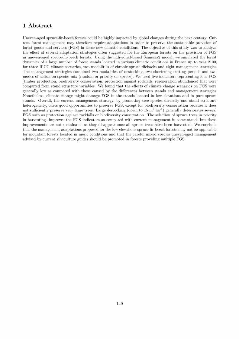
1 Abstract
Uneven-aged spruce-ir-beech forests could be highly impacted by global changes during the next century. Cur-rent forest management may therefore require adaptations in order to preserve the sustainable provision offorest goods and services (FGS) in these new climatic conditions. The objective of this study was to analyzethe efect of several adaptation strategies often suggested for the European forests on the provision of FGSin uneven-aged spruce-ir-beech forests. Using the individual-based Samsara2 model, we simulated the forestdynamics of a large number of forest stands located in various climatic conditions in France up to year 2100,for three IPCC climate scenarios, two modalities of chronic spruce diebacks and eight management strategies.The management strategies combined two modalities of destocking, two shortening cutting periods and twomodes of action on species mix (random or priority on spruce). We used ive indicators representing four FGS(timber production, biodiversity conservation, protection against rockfalls, regeneration abundance) that werecomputed from stand structure variables. We found that the efects of climate change scenarios on FGS weregenerally low as compared with those caused by the diferences between stands and management strategies.Nonetheless, climate change might damage FGS in the stands located in low elevations and in pure sprucestands. Overall, the current management strategy, by promoting tree species diversity and stand structureheterogeneity, ofers good opportunities to preserve FGS, except for biodiversity conservation because it doesnot suiciently preserve very large trees. Large destocking (down to 15 m2.ha-1) generally deteriorates severalFGS such as protection against rockfalls or biodiversity conservation. The selection of spruce trees in priorityin harvestings improves the FGS indicators as compared with current management in some stands but theseimprovements are not sustainable as they disappear once all spruce trees have been harvested. We concludethat the management adaptations proposed for the low elevations spruce-ir-beech forests may not be applicablefor mountain forests located in mesic conditions and that the careful mixed species uneven-aged managementadvised by current silviculture guides should be promoted in forests providing multiple FGS.
149
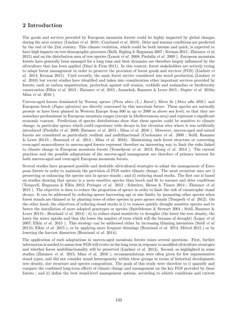
2 Introduction
The goods and services provided by European mountain forests could be highly impacted by global changesduring the next century (Lindner et al. 2010 ; Courbaud et al. 2010). Drier and warmer conditions are predictedby the end of the 21st century. This climate evolution, which could be both intense and quick, is expected tohave high impacts on tree demographic processes (Bolli, Rigling & Bugmann 2007 ; Keenan 2015 ; Zlatanov et al.2015) and on the distribution area of tree species (Lenoir et al. 2008; Piedallu et al. 2009 ). European mountainforests have generally been managed for a long time and their dynamics are therefore largely inluenced by thesilviculture that has been applied (Diaci & Firm 2011). In this context, forest stakeholders are actively tryingto adapt forest management in order to preserve the provision of forest goods and services (FGS) (Lindner etal. 2014; Keenan 2015). Until recently, the main forest service considered was wood production (Lindner etal. 2010) but recent studies have identiied and taken into consideration other important services provided byforests, such as carbon sequestration, protection against soil erosion, rockfalls and avalanches or biodiversityconservation (Elkin et al. 2013 ; Zlatanov et al. 2015 ; Irauschek, Rammer & Lexer 2015 ; Dupire et al. 2016a;Mina et al. 2016 ).
Uneven-aged forests dominated by Norway spruce (Picea abies (L.) Karst.), Silver ir (Abies alba Mill.) andEuropean beech (Fagus sylvatica) are directly concerned by this uncertain future. These species are naturallypresent or have been planted in Western Europe from 600 m up to 2000 m above sea level, so that they arenowadays predominant in European mountain ranges (except in Mediterranean area) and represent a signiicanteconomic concern. Predictions of species distributions show that these species could be sensitive to climatechange, in particular spruce which could experience wide decays in low elevation sites where it was artiiciallyintroduced (Piedallu et al. 2009; Zlatanov et al. 2015 ; Mina et al. 2016 ). Moreover, uneven-aged and mixedforests are considered as particularly resilient and multifunctional (Cordonnier et al. 2008 ; Seidl, Rammer& Lexer 2011b ; Bouriaud et al. 2014 ; Mina et al. 2016). Maintaining such forest structure or convertingeven-aged monocultures to uneven-aged forests represent therefore an interesting way to limit the risks linkedto climate change in European mountain forests (Yousefpour et al. 2013; Brang et al. 2014 ). The currentpractices and the possible adaptations of the uneven-aged management are therefore of primary interest forboth uneven-aged and even-aged European mountain forests.
Several studies have proposed possible and desirable silvicultural strategies to adapt the management of Euro-pean forests in order to maintain the provision of FGS under climate change. The most recurrent ones are i)preserving or enhancing the species mix in spruce stands ; and ii) reducing stand stocks. The irst one is basedon studies showing that spruce is a more sensitive species than beech and ir to warmer and drier conditions(Temperli, Bugmann & Elkin 2012; Peringer et al. 2013 ; Schwörer, Henne & Tinner 2014 ; Zlatanov et al.2015 ). The objective is then to reduce the proportion of spruce in order to limit the risk of catastrophic standdecays. It can be addressed by reducing spruce harvesting age or size limits, by promoting other species whenforest stands are thinned or by planting trees of other species in pure spruce stands (Temperli et al. 2012). Onthe other hand, the objectives of reducing stand stocks is i) to remove quickly drought sensitive species and tofasten the installation of more adapted genotypes or species (Spittlehouse & Stewart 2004 ; Seidl, Rammer &Lexer 2011b ; Bouriaud et al. 2014) ; ii) to reduce stand sensitivity to droughts (the lower the tree density, thelower the water uptake and thus the lower the number of trees which will die because of drought) (Legay et al.2007; Elkin et al. 2015 ). This strategy can be addressed either by increasing thinning intensities (Seidl et al.2011b; Elkin et al. 2015 ), or by applying more frequent thinnings (Bouriaud et al. 2014; Métral 2015 ) or bylowering the harvest diameters (Bouriaud et al. 2014).
The application of such adaptations in uneven-aged mountain forests raises several questions. First, furtherinformation is needed to assess how FGS will evolve in the long term in response to modiied silviculture strategiesand whether forest multifunctionality will be preserved (Lindner et al. 2014). Second, as highlighted in somestudies (Zlatanov et al. 2015; Mina et al. 2016 ), recommendations were often given for few representativestand types, and did not consider stand heterogeneity within these groups in terms of historical development,tree density, size structure and species composition. The goals of this study were therefore to i) quantify andcompare the combined long-term efects of climate change and management on the key FGS provided by theseforests ; and ii) deine the best stand-level management options, according to abiotic conditions and current
150

species compositions.
For this purpose, we analyzed the efects of the standard management strategy recommended in uneven-agedsilviculture guidelines (Gauquelin & Courbaud 2006) and of three alternative strategies of management adapta-tion on the provision of FGS : i) the reduction of the target stand density after thinning ; ii) the prioritizationon spruce in cuttings ; and iii) the shortening of time periods between cutting interventions. The irst and thesecond options represent concrete ways to apply the two recurrent adaptation strategies highlighted previously.The third one accelerates the efects of these two management options. We used the individual-based forestdynamics model Samsara2 (Lafond et al. 2014; Courbaud et al. 2015 ) to explore the efects of various climatechange and management scenarios on FGS provision. We simulated the long term dynamics of a large number(88) of forest stands for which we had previously calibrated Samsara2 (Lagarrigues et al. 2016). These standswere sampled in contrasted environmental conditions, in order to explore a wide range of situations.
We hypothesized that i) under standard management strategy, climate change would threaten the provision ofFGS in low elevation and pure spruce stands ; ii) reducing stand stocks would reduce the production loss dueto mortality but would impact negatively the service of biodiversity conservation which depends on large treesand the service of protection against natural hazards that depends on stand density ; iii) prioritizing spruce inharvestings would allow to forestall the decay of this species in response to climate change and would thus bea good alternative to standard management in stands with a high spruce proportion iv) the best managementstrategy at the stand level would depend on stand initial structure and local environmental conditions andwould therefore vary both between forests and between stands of a same forest, especially in forests spanning awide range of environmental conditions.
151
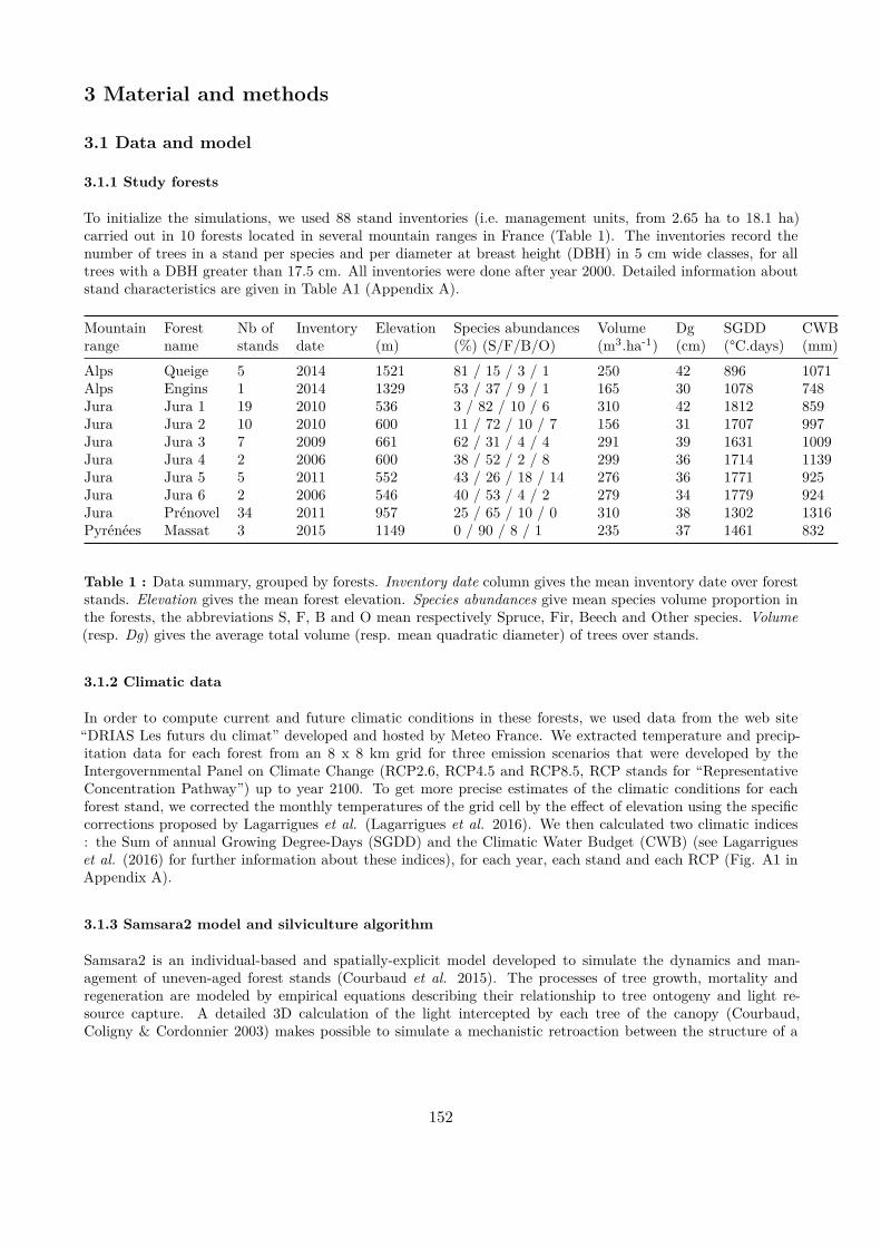
3 Material and methods
3.1 Data and model
3.1.1 Study forests
To initialize the simulations, we used 88 stand inventories (i.e. management units, from 2.65 ha to 18.1 ha)carried out in 10 forests located in several mountain ranges in France (Table 1). The inventories record thenumber of trees in a stand per species and per diameter at breast height (DBH) in 5 cm wide classes, for alltrees with a DBH greater than 17.5 cm. All inventories were done after year 2000. Detailed information aboutstand characteristics are given in Table A1 (Appendix A).
Mountainrange
Forestname
Nb ofstands
Inventorydate
Elevation(m)
Species abundances(%) (S/F/B/O)
Volume(m3.ha-1)
Dg(cm)
SGDD(°C.days)
CWB(mm)
Alps Queige 5 2014 1521 81 / 15 / 3 / 1 250 42 896 1071Alps Engins 1 2014 1329 53 / 37 / 9 / 1 165 30 1078 748Jura Jura 1 19 2010 536 3 / 82 / 10 / 6 310 42 1812 859Jura Jura 2 10 2010 600 11 / 72 / 10 / 7 156 31 1707 997Jura Jura 3 7 2009 661 62 / 31 / 4 / 4 291 39 1631 1009Jura Jura 4 2 2006 600 38 / 52 / 2 / 8 299 36 1714 1139Jura Jura 5 5 2011 552 43 / 26 / 18 / 14 276 36 1771 925Jura Jura 6 2 2006 546 40 / 53 / 4 / 2 279 34 1779 924Jura Prénovel 34 2011 957 25 / 65 / 10 / 0 310 38 1302 1316Pyrénées Massat 3 2015 1149 0 / 90 / 8 / 1 235 37 1461 832
Table 1 : Data summary, grouped by forests. Inventory date column gives the mean inventory date over foreststands. Elevation gives the mean forest elevation. Species abundances give mean species volume proportion inthe forests, the abbreviations S, F, B and O mean respectively Spruce, Fir, Beech and Other species. Volume(resp. Dg) gives the average total volume (resp. mean quadratic diameter) of trees over stands.
3.1.2 Climatic data
In order to compute current and future climatic conditions in these forests, we used data from the web site“DRIAS Les futurs du climat” developed and hosted by Meteo France. We extracted temperature and precip-itation data for each forest from an 8 x 8 km grid for three emission scenarios that were developed by theIntergovernmental Panel on Climate Change (RCP2.6, RCP4.5 and RCP8.5, RCP stands for “RepresentativeConcentration Pathway”) up to year 2100. To get more precise estimates of the climatic conditions for eachforest stand, we corrected the monthly temperatures of the grid cell by the efect of elevation using the speciiccorrections proposed by Lagarrigues et al. (Lagarrigues et al. 2016). We then calculated two climatic indices: the Sum of annual Growing Degree-Days (SGDD) and the Climatic Water Budget (CWB) (see Lagarrigueset al. (2016) for further information about these indices), for each year, each stand and each RCP (Fig. A1 inAppendix A).
3.1.3 Samsara2 model and silviculture algorithm
Samsara2 is an individual-based and spatially-explicit model developed to simulate the dynamics and man-agement of uneven-aged forest stands (Courbaud et al. 2015). The processes of tree growth, mortality andregeneration are modeled by empirical equations describing their relationship to tree ontogeny and light re-source capture. A detailed 3D calculation of the light intercepted by each tree of the canopy (Courbaud,Coligny & Cordonnier 2003) makes possible to simulate a mechanistic retroaction between the structure of a
152
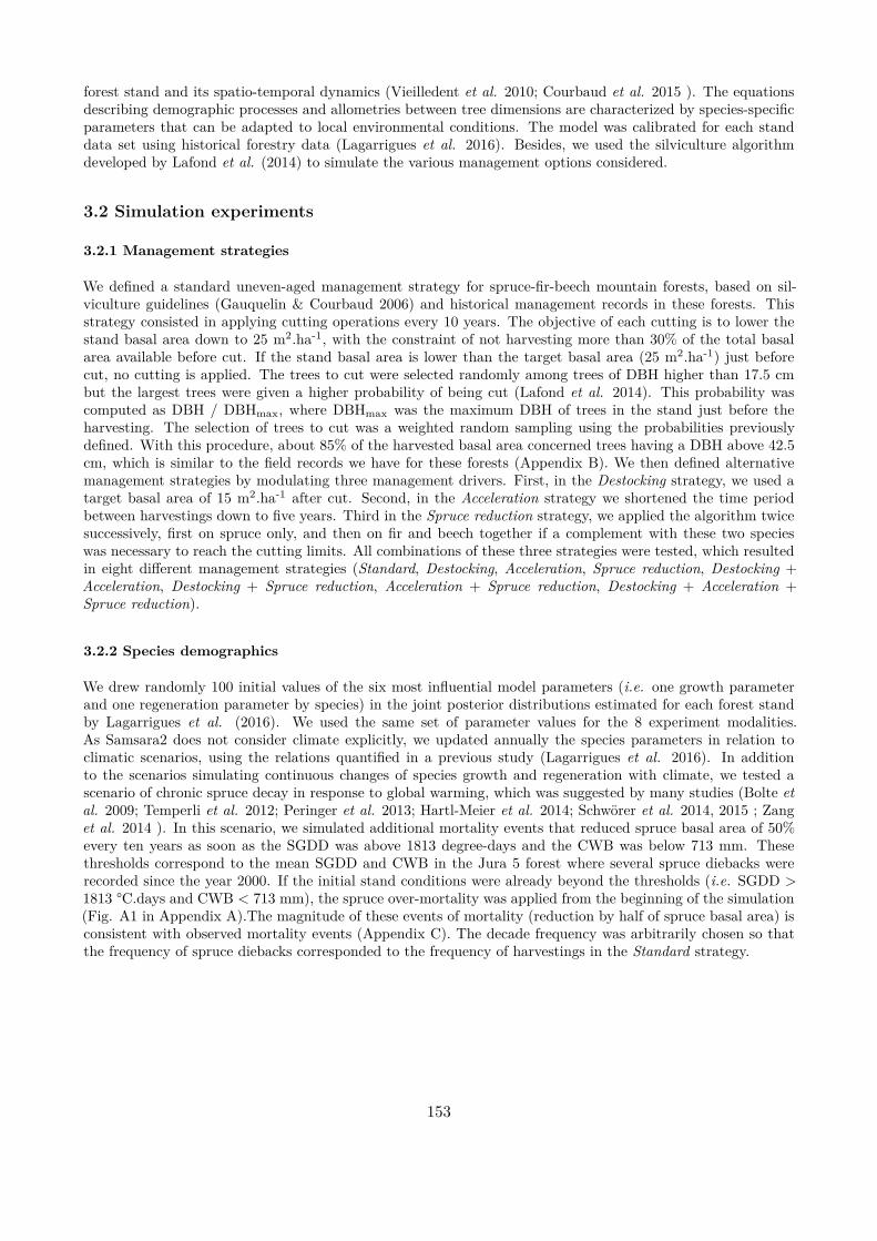
forest stand and its spatio-temporal dynamics (Vieilledent et al. 2010; Courbaud et al. 2015 ). The equationsdescribing demographic processes and allometries between tree dimensions are characterized by species-speciicparameters that can be adapted to local environmental conditions. The model was calibrated for each standdata set using historical forestry data (Lagarrigues et al. 2016). Besides, we used the silviculture algorithmdeveloped by Lafond et al. (2014) to simulate the various management options considered.
3.2 Simulation experiments
3.2.1 Management strategies
We deined a standard uneven-aged management strategy for spruce-ir-beech mountain forests, based on sil-viculture guidelines (Gauquelin & Courbaud 2006) and historical management records in these forests. Thisstrategy consisted in applying cutting operations every 10 years. The objective of each cutting is to lower thestand basal area down to 25 m2.ha-1, with the constraint of not harvesting more than 30% of the total basalarea available before cut. If the stand basal area is lower than the target basal area (25 m2.ha-1) just beforecut, no cutting is applied. The trees to cut were selected randomly among trees of DBH higher than 17.5 cmbut the largest trees were given a higher probability of being cut (Lafond et al. 2014). This probability wascomputed as DBH / DBHmax, where DBHmax was the maximum DBH of trees in the stand just before theharvesting. The selection of trees to cut was a weighted random sampling using the probabilities previouslydeined. With this procedure, about 85% of the harvested basal area concerned trees having a DBH above 42.5cm, which is similar to the ield records we have for these forests (Appendix B). We then deined alternativemanagement strategies by modulating three management drivers. First, in the Destocking strategy, we used atarget basal area of 15 m2.ha-1 after cut. Second, in the Acceleration strategy we shortened the time periodbetween harvestings down to ive years. Third in the Spruce reduction strategy, we applied the algorithm twicesuccessively, irst on spruce only, and then on ir and beech together if a complement with these two specieswas necessary to reach the cutting limits. All combinations of these three strategies were tested, which resultedin eight diferent management strategies (Standard, Destocking, Acceleration, Spruce reduction, Destocking +Acceleration, Destocking + Spruce reduction, Acceleration + Spruce reduction, Destocking + Acceleration +Spruce reduction).
3.2.2 Species demographics
We drew randomly 100 initial values of the six most inluential model parameters (i.e. one growth parameterand one regeneration parameter by species) in the joint posterior distributions estimated for each forest standby Lagarrigues et al. (2016). We used the same set of parameter values for the 8 experiment modalities.As Samsara2 does not consider climate explicitly, we updated annually the species parameters in relation toclimatic scenarios, using the relations quantiied in a previous study (Lagarrigues et al. 2016). In additionto the scenarios simulating continuous changes of species growth and regeneration with climate, we tested ascenario of chronic spruce decay in response to global warming, which was suggested by many studies (Bolte etal. 2009; Temperli et al. 2012; Peringer et al. 2013; Hartl-Meier et al. 2014; Schwörer et al. 2014, 2015 ; Zanget al. 2014 ). In this scenario, we simulated additional mortality events that reduced spruce basal area of 50%every ten years as soon as the SGDD was above 1813 degree-days and the CWB was below 713 mm. Thesethresholds correspond to the mean SGDD and CWB in the Jura 5 forest where several spruce diebacks wererecorded since the year 2000. If the initial stand conditions were already beyond the thresholds (i.e. SGDD >1813 °C.days and CWB < 713 mm), the spruce over-mortality was applied from the beginning of the simulation(Fig. A1 in Appendix A).The magnitude of these events of mortality (reduction by half of spruce basal area) isconsistent with observed mortality events (Appendix C). The decade frequency was arbitrarily chosen so thatthe frequency of spruce diebacks corresponded to the frequency of harvestings in the Standard strategy.
153
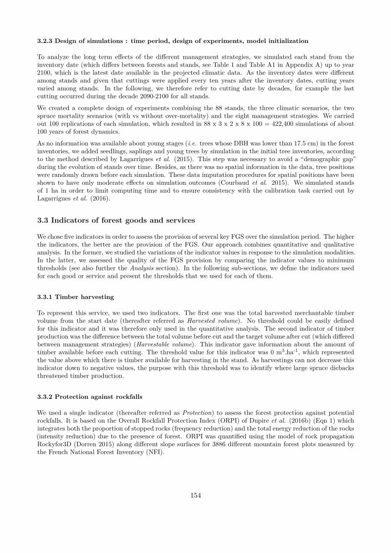
3.2.3 Design of simulations : time period, design of experiments, model initialization
To analyze the long term efects of the diferent management strategies, we simulated each stand from theinventory date (which difers between forests and stands, see Table 1 and Table A1 in Appendix A) up to year2100, which is the latest date available in the projected climatic data. As the inventory dates were diferentamong stands and given that cuttings were applied every ten years after the inventory dates, cutting yearsvaried among stands. In the following, we therefore refer to cutting date by decades, for example the lastcutting occurred during the decade 2090-2100 for all stands.
We created a complete design of experiments combining the 88 stands, the three climatic scenarios, the twospruce mortality scenarios (with vs without over-mortality) and the eight management strategies. We carriedout 100 replications of each simulation, which resulted in 88 x 3 x 2 x 8 x 100 = 422,400 simulations of about100 years of forest dynamics.
As no information was available about young stages (i.e. trees whose DBH was lower than 17.5 cm) in the forestinventories, we added seedlings, saplings and young trees by simulation in the initial tree inventories, accordingto the method described by Lagarrigues et al. (2015). This step was necessary to avoid a “demographic gap”during the evolution of stands over time. Besides, as there was no spatial information in the data, tree positionswere randomly drawn before each simulation. These data imputation procedures for spatial positions have beenshown to have only moderate efects on simulation outcomes (Courbaud et al. 2015). We simulated standsof 1 ha in order to limit computing time and to ensure consistency with the calibration task carried out byLagarrigues et al. (2016).
3.3 Indicators of forest goods and services
We chose ive indicators in order to assess the provision of several key FGS over the simulation period. The higherthe indicators, the better are the provision of the FGS. Our approach combines quantitative and qualitativeanalysis. In the former, we studied the variations of the indicator values in response to the simulation modalities.In the latter, we assessed the quality of the FGS provision by comparing the indicator values to minimumthresholds (see also further the Analysis section). In the following sub-sections, we deine the indicators usedfor each good or service and present the thresholds that we used for each of them.
3.3.1 Timber harvesting
To represent this service, we used two indicators. The irst one was the total harvested merchantable timbervolume from the start date (thereafter referred as Harvested volume). No threshold could be easily deinedfor this indicator and it was therefore only used in the quantitative analysis. The second indicator of timberproduction was the diference between the total volume before cut and the target volume after cut (which diferedbetween management strategies) (Harvestable volume). This indicator gave information about the amount oftimber available before each cutting. The threshold value for this indicator was 0 m3.ha-1, which representedthe value above which there is timber available for harvesting in the stand. As harvestings can not decrease thisindicator down to negative values, the purpose with this threshold was to identify where large spruce diebacksthreatened timber production.
3.3.2 Protection against rockfalls
We used a single indicator (thereafter referred as Protection) to assess the forest protection against potentialrockfalls. It is based on the Overall Rockfall Protection Index (ORPI) of Dupire et al. (2016b) (Eqn 1) whichintegrates both the proportion of stopped rocks (frequency reduction) and the total energy reduction of the rocks(intensity reduction) due to the presence of forest. ORPI was quantiied using the model of rock propagationRockyfor3D (Dorren 2015) along diferent slope surfaces for 3886 diferent mountain forest plots measured bythe French National Forest Inventory (NFI).
154
In Eqn. 1, slopeLength is the forest length along the slope, Ecumforest(slopeLength) is the cumulated energy ofrocks passing the distance slopeLength through the forest and Ecumnoforest(slopeLength) is the cumulated energyof rocks passing the distance slopeLength along the same slope but without forest.
The ORPI takes value between 0 (low protection) and 100 (high protection). Our Protection indicator wasORPI(100 m) for 1 m3 rock volumes. To limit the computing time, we did not use the rock propagation modelin this study. We rather used simpliied relations between ORPI, the mean diameter (Dm) and the basal area(G) of trees with DBH above 7.5 cm in the NFI data. ORPI was positively correlated with G and negativelywith Dm, with strong interactions between these two factors. We therefore selected ive ORPI classes (<0% ;80-90% ; 90-95% ; 95-99% ; >99%) and we calibrated the four linear equations of type Dm = a x G + b thatpartitioned the best these ive classes (Fig. D1 in Appendix D). We inally estimated the ORPI classes for oursimulations using Dm, G and the coeicients of these equations. We chose 90% as a threshold value for thisindicator, which corresponds to a reduction of 90% of the rockfall hazard by the forest.
3.3.3 Biodiversity conservation
We used the abundance of very large trees (DBH > 77.5 cm) as an indirect indicator of the biodiversityconservation service (referred as Biodiversity in the following). Large trees have been shown to have a positiveefect on biodiversity because they often carry tree microhabitats such as hollows, cracks or areas of exposedwood that can be used as feeding, breeding or roosting places by a great variety of taxa such as fungi, insects,bats, birds or lichens (Larrieu, Cabanettes & Delarue 2011; Regnery et al. 2013 ). They also produce largepieces of dead wood used by saproxylic species (Siitonen 2001), and they participate to a vertically heterogeneousstand structure that favors a diversity of niches in the forest stand (Ishii, Tanabe & Hiura 2004 ; Nascimbene etal. 2008). The threshold value for this indicator was 5 trees with DBH > 77.5 cm, which was the limit betweenadult and mature stands deined by Fuhr et al. (2015).
3.3.4 Regeneration abundance
Strictly speaking, regeneration is neither a good nor a service, but regeneration abundance (thereafter simplyreferred as Regeneration) gives information about the forest renewal potential and resilience to disturbance(Cordonnier et al. 2008). Regeneration abundance represents therefore a key indicator of FGS sustainability.Following Gauquelin and Courbaud (2006), we quantiied regeneration abundance by computing the proportionof ground area covered by the young trees. We subdivided the simulated plot (1 ha) in 100 square metersground cells (so 100 cells in the plot) and the indicator was the proportion of cells having more than half oftheir surface covered by the crown of small trees (i.e. height less than 8.75 m). Following the guidelines givenby Gauquelin and Courbaud (2006), we used a threshold value of 5% for this indicator.
155

3.4 Analysis
3.4.1 Vulnerability of FGS to climate change under the Standard strategy
In this irst part of the analysis, we aimed at determining if the FGS might be threatened by climate change insome stands under the Standard strategy.
3.4.1.1 Variations of FGS due to climate change under the Standard strategy
First, we selected only the simulations concerning this management strategy and we analyzed the interactiveefects of climate change and spruce over-mortality scenarios on FGS. For that purpose, we used the scenarioRCP2.6 without spruce over-mortality as a reference, and we compared it with the results obtained with (1) theclimate change scenario RCP8.5 without spruce over-mortality, (2) the climate change scenario RCP2.6 withspruce over-mortality and (3) the climate change scenario RCP8.5 with spruce over-mortality. Here, we selectedonly the year after the last cut (decade 2090-2100) and we averaged indicator values over the 100 replicates.
3.4.1.2 Evolution of FGS quality under the Standard strategy
We then used more qualitative considerations to detect in which stands the FGS indicators did not reach qualityobjectives by the year 2100 under the Standard strategy. We deined the quality objectives of the indicators atstand level by computing the proportion of simulations above the indicator thresholds. We considered that theindicator reached the quality objective if more than 90% of the 600 simulations (3 climate change scenarios x2 spruce over-mortality scenarios x 100 replicates) were above the indicator threshold. We also tested diferentacceptance rates (95% or 100%) to assess the sensitivity of the results to this threshold. We determined whetherthe indicators reached the quality objectives at the start and end dates, to assess the trajectory of the indicatorduring the simulations.
3.4.2 Efects of management strategies on FGS
In this second part of the analysis, we analyzed the efects of alternative management strategies on FGS andassessed whether they improved FGS when they were threatened by climate change under the Standard strategy.
3.4.2.1 ANOVA on the indicator values
First, we carried out an analysis of variance (ANOVA) to compare the efects of the diverse sources of variability(stands, climate change scenarios, spruce over-mortality scenarios and management strategies) on the ive FGSindicators. The dependent variables were the diferences of indicators between the year after the last cut (decade2090-2100) and the year after cut within the decade 2020-2030. All interactions between factors were includedin the analysis.
3.4.2.2 Overall efects of management strategies on FGS
We summarized the simulated data by averaging over all stands, selecting only the most severe scenario, i.e.the RCP8.5 climate change scenario with spruce over-mortality. We only considered the proper efects of thediferent strategies (Standard strategy or alternatively the Destocking, the Acceleration or the Spruce reductionstrategy alone) and ignored the management strategies that were made of a combination of these modalities.
3.4.3 Selection of the best management strategy for each stand
In this third part of the analyses, the objective was to select the management strategy that ofered the besttrade-of between the diferent FGS, for each stand independently, and then to assess the improvement broughtby this best strategy on FGS compared with the Standard strategy.
156

3.4.3.1 Ranking of management strategies
We assigned rank values to management strategies, which were successive entire values where the best strategywas attributed the highest rank and the worst strategy the lowest rank. We computed these rankings for eachFGS indicator and each simulation (i.e. 600 rankings by indicator for each stand). The rank values were thenaveraged to obtain a global rank by stand and by management strategy, and the best management strategy fora stand was deined as the strategy with the highest global rank.
3.4.3.2 FGS quality under the best management strategy
Finally, we aimed at assessing whether the best management strategy provided signiicant improvement for FGSand whether it resulted in losses for some of the FGS. For that purpose, we compared the qualitative evaluationsof the indicators with the ones obtained with the Standard strategy.
157
4 Results
4.1 Vulnerability of FGS to climate change under the Standard strategy
4.1.1 Variations of FGS to climate change under the Standard strategy
Without spruce over-mortality (SOM), the various climate change (CC) scenarios lead to similar values of theFGS indicators (Fig. 1, left column). In contrast, applying spruce over-mortality on the RCP2.6 CC scenarioresulted in signiicant changes for some stands (black dots in the middle column of the Fig. 1). Finally, combiningthe SOM and the more severe CC scenario (RCP8.5) generally resulted in signiicant damaging changes on theindicators, as the inter-quartile ranges were larger for all indicators or shifted downwards (Harvested volume,Protection and Regeneration) (Fig. 1, right column) as compared with the efects of CC alone (Fig. 1, leftcolumn). Focusing on the outliers, we observed that the damaging efects were either magniied by a severeglobal warming (the outliers present in CC x SOM and not in SOM only) or reduced (the outliers present inSOM and not in CC x SOM for Harvested volume). The former case mainly occurred in spruce stands (e.g.Queige forest), whereas the latter was observed in mixed ir-spruce stands (Jura 3 forest). This last situationoccurred in our simulations because ir growth was enhanced by higher temperature. The spruce dead treeswere thus more easily replaced by ir trees, which preserved the harvestings in these stands.
158
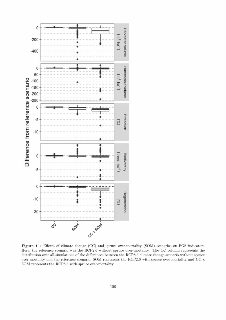
Figure 1 : Efects of climate change (CC) and spruce over-mortality (SOM) scenarios on FGS indicators.Here, the reference scenario was the RCP2.6 without spruce over-mortality. The CC column represents thedistribution over all simulations of the diferences between the RCP8.5 climate change scenario without spruceover-mortality and the reference scenario, SOM represents the RCP2.6 with spruce over-mortality and CC xSOM represents the RCP8.5 with spruce over-mortality.
159

4.1.2 Evolution of FGS quality under the Standard strategy
Except for Biodiversity, the indicators generally reached the quality objectives in our forest stands at the enddates (Table 2 and the complete stand level results in Appendix D). The diferent acceptance rates to assessthe quality objectives (90, 95 or 100%) gave qualitatively similar results.
We then analyzed the initial stand properties that had an inluence on the quality of the indicators at the enddate of the simulation, indicator by indicator.
4.1.2.1 Harvestable volume
Out of the 88 studied stands, the indicator Harvestable volume was below the objective for only 5 stands (Jura 2stand 2, Jura 3 stand 3, and stands C, 6 and 32 in Queige). The Queige and Jura 3 stands combined a particularhigh spruce proportion and a low ir growth rate, so that the spruce over-mortality was hardly compensatedby ir, degrading thus the stock volume available for harvesting. The Jura 2 forest was particular in that theinitial stocks were low (under 200 m3.ha-1, and less than 150 m3.ha-1 in the stand 2) and, moreover, the irgrowth rate was weak in the stand 2, so that the stock volume remained low in all simulations. The Standardstrategy allowed to reach the quality objective for stands C and K in Queige and the stand 2 in Jura 2, wherecompanion species (i.e. other than spruce) proportion was suiciently high (more than 15 %), and reduced theindicator below the quality objective in the other Queige stands (32 and 6) and the Jura 3 stands where spruceproportion was high.
4.1.2.2 Protection
The protection indicator was only below the quality objective for three stands (Jura 1 stand 19, Jura 5 stand18 and Queige stand 6), but several other stands had some simulations under the threshold in the Jura 1forest. These stands are characterized by a high quadratic mean diameter (above 40 cm), resulting in a lowerprobability of impacts between rocks and trees and therefore a lower capability in reducing rockfall hazard whenstem density was strongly lowered (for instance in simulations with spruce over-mortality). In all these cases,the Standard strategy reduced this indicator below the quality objective, because the tree density was loweredby both spruce over-mortality and harvestings.
4.1.2.3 Regeneration
This indicator always reached the quality objective but some simulations had low indicator values for the stand19 in Jura 5. This stand is located in the warmest forest and had a higher spruce proportion than other standsin the same forest, which resulted in high impacts on stand dynamics caused by spruce over-mortality. TheStandard strategy damaged this indicator in this stand, as the quality objective was reached at the start dateand not at the end date under this management strategy. The inverse situation occurred in the low stock standsof the Jura 2 forest, because the Standard strategy did not harvest trees while the stock did not have reached250 m3.ha-1 and thus raised the indicator above the quality objective.
4.1.2.4 Biodiversity
Concerning Biodiversity, 39 stands did not reach the quality objective, particularly in the Engins, Jura 2, Massatand Queige forests where almost all stands were concerned (Table 2). The environmental conditions in the forestJura 2 caused low fertility for all tree species (thin soil and/or non optimal climate), which explained partiallywhy very large trees are currently scarce in these forests and remain scarce under the Standard strategy. InMassat, the tree growth rates were low, so that trees were often cut before reaching the maturity DBH threshold(77.5 cm). In the other forests, this indicator was below the quality objective where there are high spruceproportions, low quadratic diameters and/or low ir growth rates. Still, the Standard strategy, by harvestingtrees all over the tree size range rather than by focusing on the largest ones, generally allowed this indicator toreach the quality objective during the simulation in these forests (Appendix D).
160
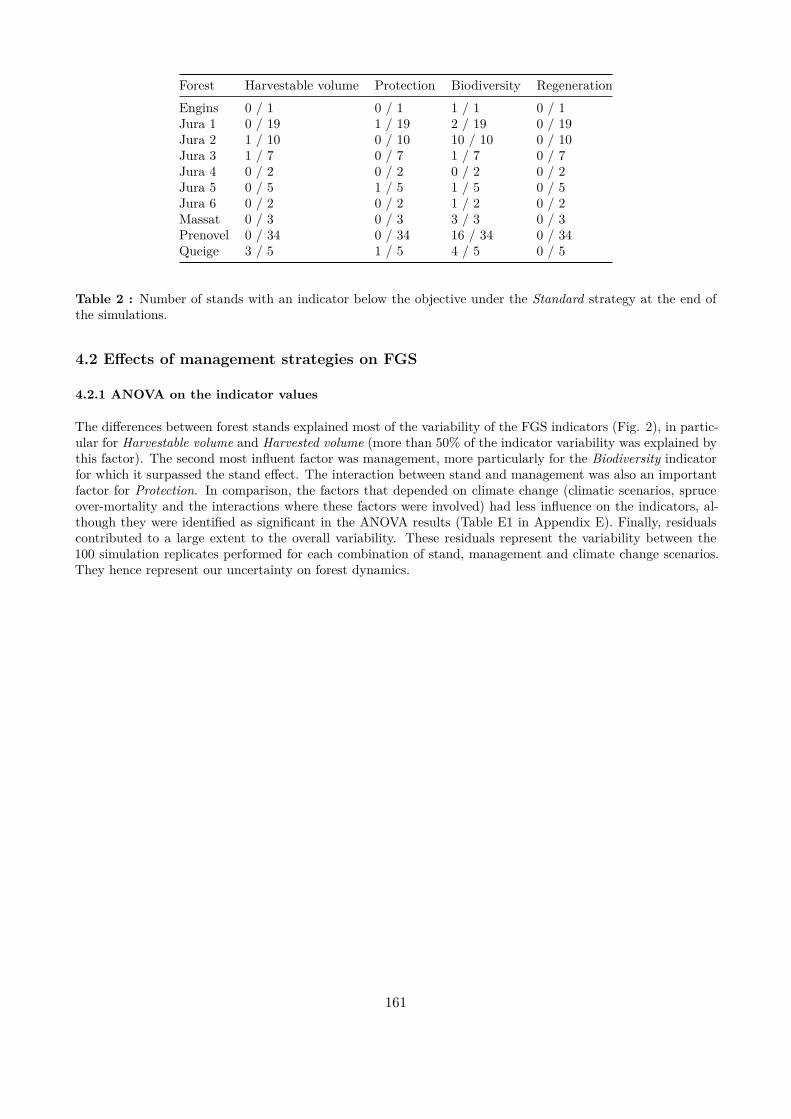
Forest Harvestable volume Protection Biodiversity RegenerationEngins 0 / 1 0 / 1 1 / 1 0 / 1Jura 1 0 / 19 1 / 19 2 / 19 0 / 19Jura 2 1 / 10 0 / 10 10 / 10 0 / 10Jura 3 1 / 7 0 / 7 1 / 7 0 / 7Jura 4 0 / 2 0 / 2 0 / 2 0 / 2Jura 5 0 / 5 1 / 5 1 / 5 0 / 5Jura 6 0 / 2 0 / 2 1 / 2 0 / 2Massat 0 / 3 0 / 3 3 / 3 0 / 3Prenovel 0 / 34 0 / 34 16 / 34 0 / 34Queige 3 / 5 1 / 5 4 / 5 0 / 5
Table 2 : Number of stands with an indicator below the objective under the Standard strategy at the end ofthe simulations.
4.2 Efects of management strategies on FGS
4.2.1 ANOVA on the indicator values
The diferences between forest stands explained most of the variability of the FGS indicators (Fig. 2), in partic-ular for Harvestable volume and Harvested volume (more than 50% of the indicator variability was explained bythis factor). The second most inluent factor was management, more particularly for the Biodiversity indicatorfor which it surpassed the stand efect. The interaction between stand and management was also an importantfactor for Protection. In comparison, the factors that depended on climate change (climatic scenarios, spruceover-mortality and the interactions where these factors were involved) had less inluence on the indicators, al-though they were identiied as signiicant in the ANOVA results (Table E1 in Appendix E). Finally, residualscontributed to a large extent to the overall variability. These residuals represent the variability between the100 simulation replicates performed for each combination of stand, management and climate change scenarios.They hence represent our uncertainty on forest dynamics.
161
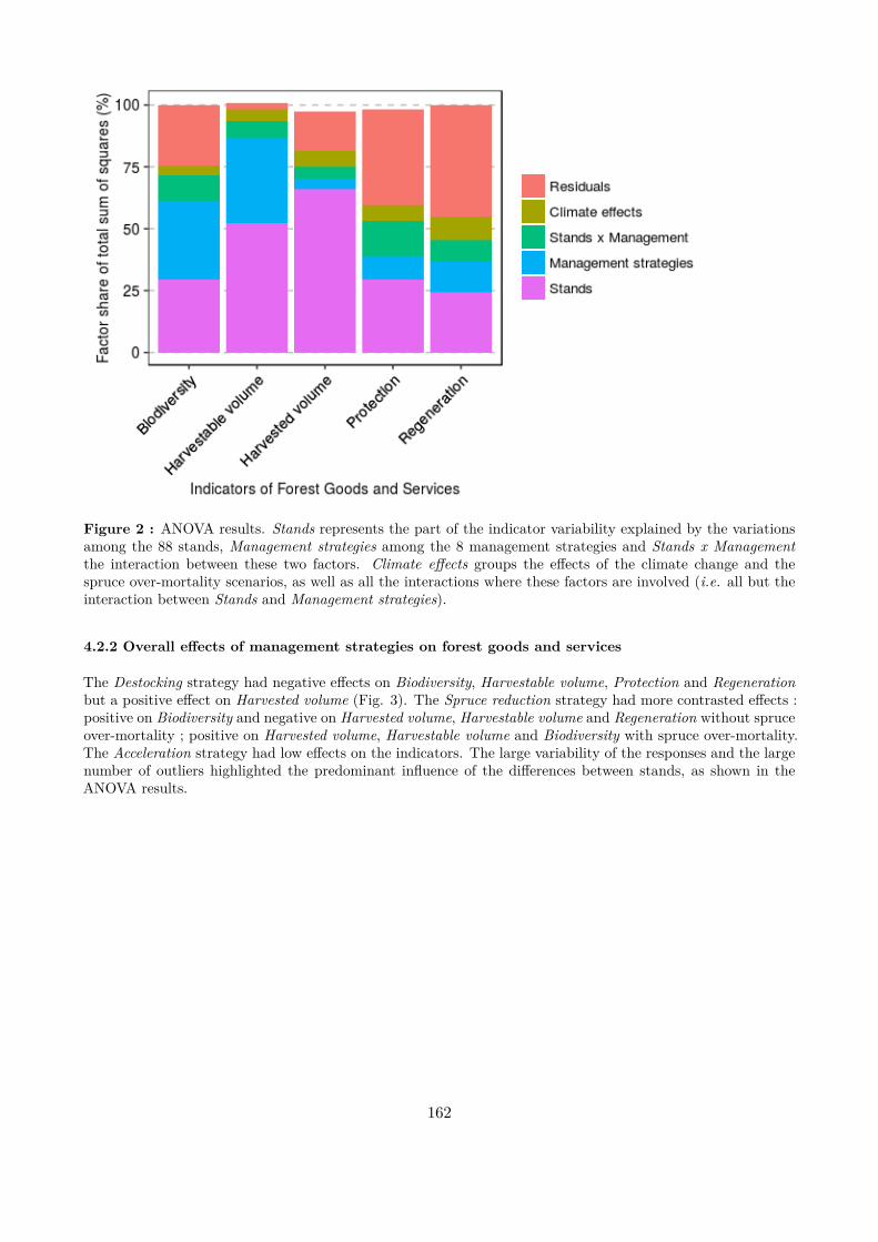
Figure 2 : ANOVA results. Stands represents the part of the indicator variability explained by the variationsamong the 88 stands, Management strategies among the 8 management strategies and Stands x Managementthe interaction between these two factors. Climate efects groups the efects of the climate change and thespruce over-mortality scenarios, as well as all the interactions where these factors are involved (i.e. all but theinteraction between Stands and Management strategies).
4.2.2 Overall efects of management strategies on forest goods and services
The Destocking strategy had negative efects on Biodiversity, Harvestable volume, Protection and Regenerationbut a positive efect on Harvested volume (Fig. 3). The Spruce reduction strategy had more contrasted efects :positive on Biodiversity and negative on Harvested volume, Harvestable volume and Regeneration without spruceover-mortality ; positive on Harvested volume, Harvestable volume and Biodiversity with spruce over-mortality.The Acceleration strategy had low efects on the indicators. The large variability of the responses and the largenumber of outliers highlighted the predominant inluence of the diferences between stands, as shown in theANOVA results.
162
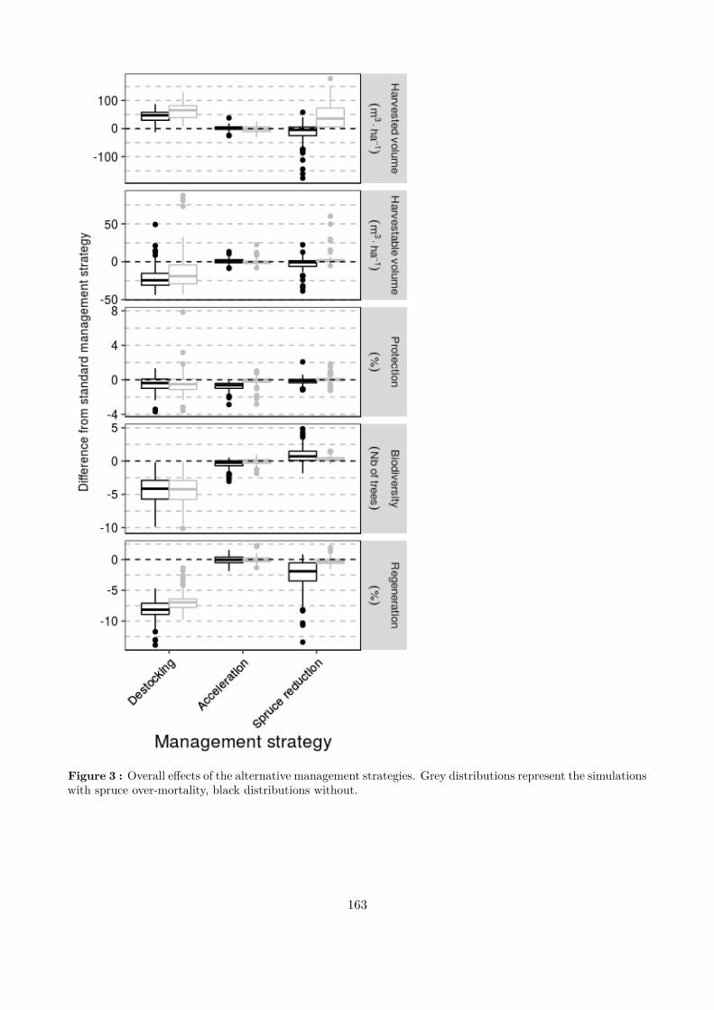
Figure 3 : Overall efects of the alternative management strategies. Grey distributions represent the simulationswith spruce over-mortality, black distributions without.
163
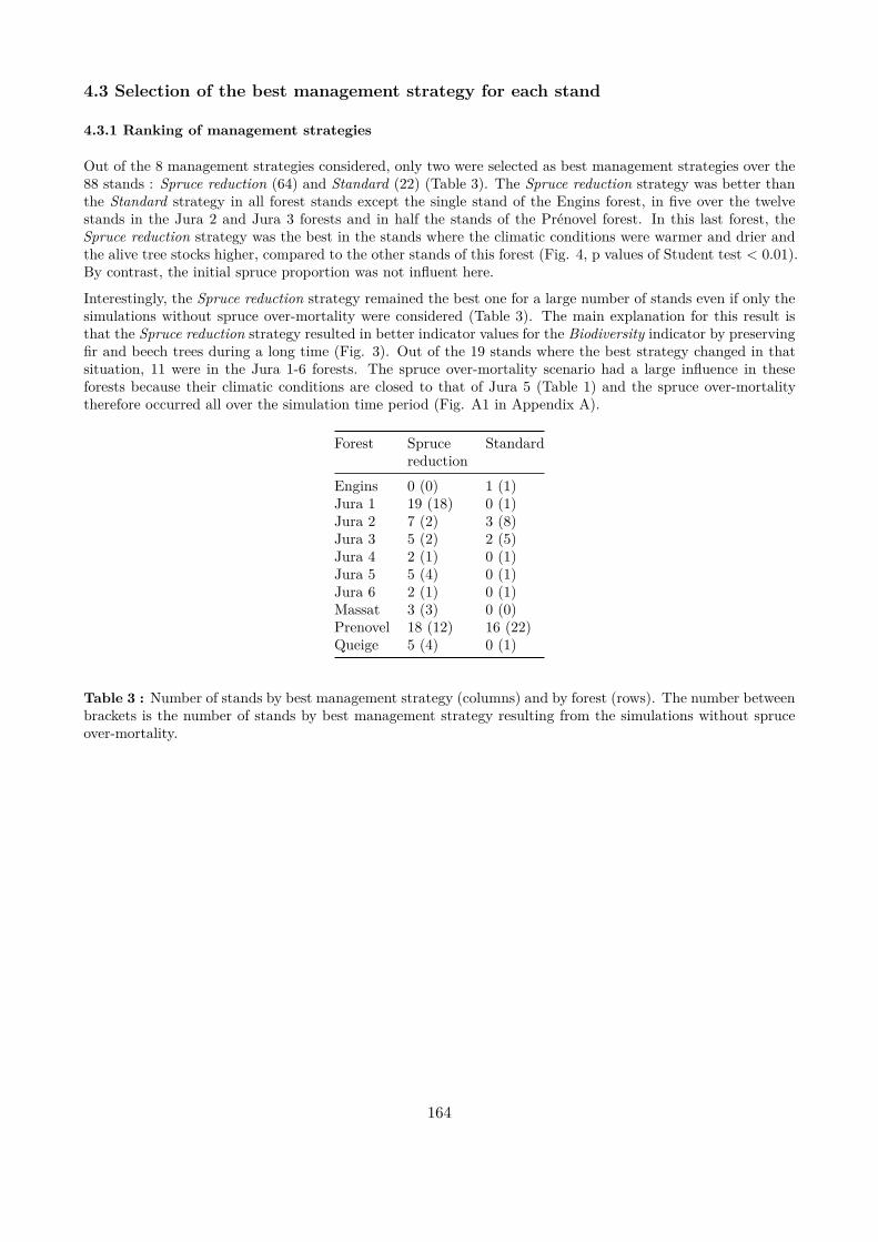
4.3 Selection of the best management strategy for each stand
4.3.1 Ranking of management strategies
Out of the 8 management strategies considered, only two were selected as best management strategies over the88 stands : Spruce reduction (64) and Standard (22) (Table 3). The Spruce reduction strategy was better thanthe Standard strategy in all forest stands except the single stand of the Engins forest, in ive over the twelvestands in the Jura 2 and Jura 3 forests and in half the stands of the Prénovel forest. In this last forest, theSpruce reduction strategy was the best in the stands where the climatic conditions were warmer and drier andthe alive tree stocks higher, compared to the other stands of this forest (Fig. 4, p values of Student test < 0.01).By contrast, the initial spruce proportion was not inluent here.
Interestingly, the Spruce reduction strategy remained the best one for a large number of stands even if only thesimulations without spruce over-mortality were considered (Table 3). The main explanation for this result isthat the Spruce reduction strategy resulted in better indicator values for the Biodiversity indicator by preservingir and beech trees during a long time (Fig. 3). Out of the 19 stands where the best strategy changed in thatsituation, 11 were in the Jura 1-6 forests. The spruce over-mortality scenario had a large inluence in theseforests because their climatic conditions are closed to that of Jura 5 (Table 1) and the spruce over-mortalitytherefore occurred all over the simulation time period (Fig. A1 in Appendix A).
Forest Sprucereduction
Standard
Engins 0 (0) 1 (1)Jura 1 19 (18) 0 (1)Jura 2 7 (2) 3 (8)Jura 3 5 (2) 2 (5)Jura 4 2 (1) 0 (1)Jura 5 5 (4) 0 (1)Jura 6 2 (1) 0 (1)Massat 3 (3) 0 (0)Prenovel 18 (12) 16 (22)Queige 5 (4) 0 (1)
Table 3 : Number of stands by best management strategy (columns) and by forest (rows). The number betweenbrackets is the number of stands by best management strategy resulting from the simulations without spruceover-mortality.
164
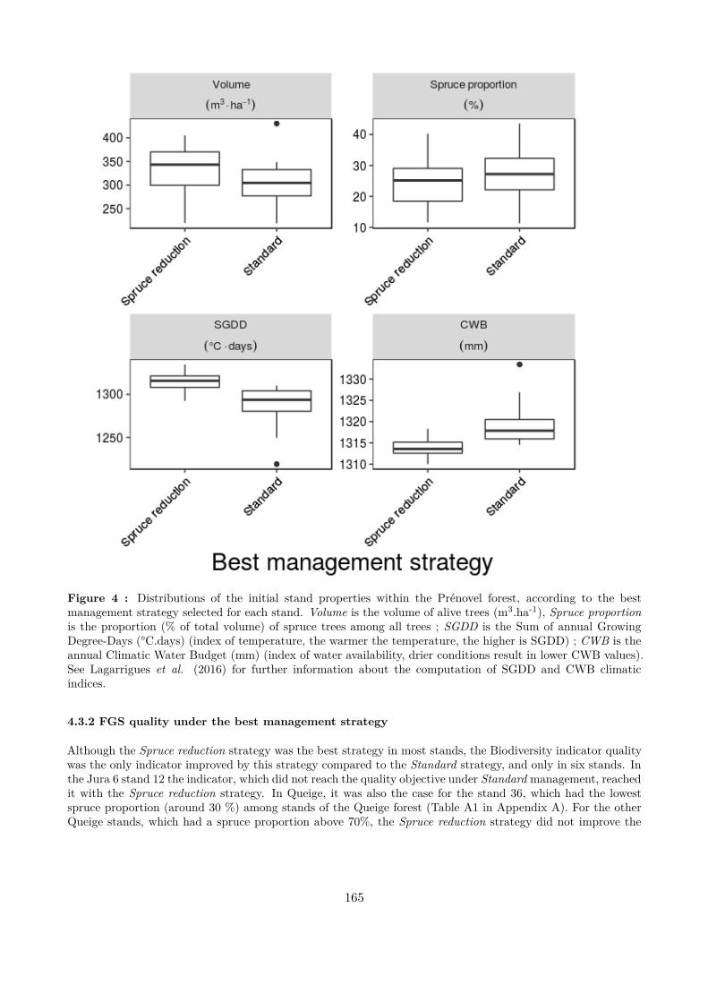
Figure 4 : Distributions of the initial stand properties within the Prénovel forest, according to the bestmanagement strategy selected for each stand. Volume is the volume of alive trees (m3.ha-1), Spruce proportionis the proportion (% of total volume) of spruce trees among all trees ; SGDD is the Sum of annual GrowingDegree-Days (°C.days) (index of temperature, the warmer the temperature, the higher is SGDD) ; CWB is theannual Climatic Water Budget (mm) (index of water availability, drier conditions result in lower CWB values).See Lagarrigues et al. (2016) for further information about the computation of SGDD and CWB climaticindices.
4.3.2 FGS quality under the best management strategy
Although the Spruce reduction strategy was the best strategy in most stands, the Biodiversity indicator qualitywas the only indicator improved by this strategy compared to the Standard strategy, and only in six stands. Inthe Jura 6 stand 12 the indicator, which did not reach the quality objective under Standard management, reachedit with the Spruce reduction strategy. In Queige, it was also the case for the stand 36, which had the lowestspruce proportion (around 30 %) among stands of the Queige forest (Table A1 in Appendix A). For the otherQueige stands, which had a spruce proportion above 70%, the Spruce reduction strategy did not improve the
165

quality of the Biodiversity indicator. In Prénovel, the Spruce reduction strategy allowed the indicator to reachthe quality objective only in stands with a high spruce proportion, because ir and beech were thus preservedfrom cuttings. In all other cases, the indicator quality was not changed by the Spruce reduction strategy : thestands that did not reach the quality objective for an indicator under the Standard strategy remained as suchunder the Spruce reduction strategy, and similarly for the stands that reached the quality objective.
166
5 Discussion
5.1 Relative importance of factors afecting FGS
The diferences between climate change scenarios resulted in low variations of the FGS indicators. The mainexplanation for that result is that climate inluence was low in our model, which was due to the results of themodel calibration done in a previous study (Lagarrigues et al. 2016). This is largely related to the fact that mostof the studied forests are located in the core of the spruce-ir-beech distribution area, where the climatic stressis presently relatively small for these species and should become more critical only progressively in the futurecentury. On the other hand, the spruce over-mortality scenario signiicantly damaged the FGS in the warmestand driest conditions of the study sites (Fig. 1), especially in pure spruce stands. These results highlight thatclimate has only marginal efects on FGS in mesic conditions but also that large damaging impacts could beobserved in forests that will experience climatic conditions outside these mesic conditions, especially if speciessensitive to warm and dry conditions such as spruce are abundant in these forests.
In our study, we found that some factors afect more than climate the forest goods and services provided byEuropean uneven-aged mountain forests (Fig. 2). First of all, local variations of environmental conditions,species composition, size structure and management history have a great inluence on the current and futureprovision of FGS. Adaptation of forest management should thus take into account in priority the speciic featuresof forest stands, even within a same forest. Taking into account bioclimatic zones has already been done instudies dealing with the adaptation of forest management to climate change (Lindner et al. 2010, 2014 ) butthe stand-level speciicities had generally not been considered (Zlatanov et al. 2015; Mina et al. 2016 ). Wedemonstrated here that they can be of major importance in uneven-aged mountain forests. As our model wascalibrated locally for each stand using historical data (Lagarrigues et al. 2016), our approach was particularlyrelevant to address this issue.
We also showed that, in these forests, management can greatly inluence the FGS. This result suggests thatforest managers have the opportunity to maintain or improve FGS in a context of global change, but on theother hand, they have an important responsibility concerning the evolution of these forests, as FGS can bedeteriorated when inappropriate management strategies are applied (such as the large reduction of stand stockexplored in this study).
Important spruce mortality events caused by bark beetle outbreaks have been observed in many studies, showingthat drought stress can allow these insects to cause large damages (Schlyter et al. 2006; Bolte et al. 2009 ;Netherer et al. 2015 ). In our study, the exploratory spruce over-mortality that we simulated had also animportant impact in pure spruce stands but a negligible impact in well-mixed stands. As the latter werepredominant in our study area, the climate inluence was overall low in our results (Fig. 2) (see also Mina etal. (2016) for similar low inluence of climate in a large range of European mountain forests), in contrast toother studies made on forests where spruce is much more abundant (Elkin et al. 2013 ; Zlatanov et al. 2015 ;Irauschek et al. 2015).
5.2 The current management strategy might preserve FGS in most forest stands
Our FGS indicators generally reached the quality objectives at the beginning of the simulations (i.e. the currentforest states) and remained as such at the end of the simulations in most cases under climate change (Table2). This result conirmed that a well-reasoned uneven-aged management can sustain many FGS (Bouriaud etal. 2014 ; Härtl et al. 2015; Mina et al. 2016 ). However, the forest biodiversity conservation service is animportant exception and alternative management options should be considered to improve this service.
In forests where trees can grow up to very large diameters, our Spruce reduction strategy was better thanthe Standard strategy for that indicator since it preserved ir and beech trees which could then grow a verylong time before being cut. Obviously, this efect occurs only temporarily (until there is no longer enoughspruce trees to cut), so that this strategy can not be considered as sustainable. An intentional retention ofoldest or largest trees would improve this biodiversity indicator, although it would impose to accept a trade-of
167
issue between biodiversity conservation and timber harvesting (Lafond, Cordonnier & Courbaud 2015). Moregenerally, no management strategy can simultaneously maximize both services at the stand level, so that largetree retention should also be considered at the landscape level (Mina et al. 2016) (see also further the discussionabout the FGS indicators that we used). Moreover, in forests such as Jura 2 where trees hardly grow up tovery large diameters, the Standard strategy is the least damaging solution for biodiversity conservation, sincethe alternative management strategies explored in this study did not improve signiicantly this indicator (Fig.3).
Although the prioritization of spruce in harvestings was identiied as the best strategy in most cases in ourstudy, it resulted in signiicant improvements of the indicators only in some cases. In particular, the standslocated in the warmest conditions in the Prénovel forest as well as the well-mixed Queige stands beneited fromthis management strategy. This result illustrates that diferent management strategies can be optimal in asame forest. Nevertheless, if this strategy preserved the wood production quantitatively, it also resulted in aqualitative shift over time, as timber is essentially obtained from spruce trees in the beginning and from irand beech at the end of the simulations. This shift may be problematic for forest managers since spruce treesproduces a better wood quality than ir or beech.
For some stands, several indicators were identiied as vulnerable with the Standard strategy and none of thealternative strategies that we explored improved the situation (for example for the Queige pure spruce stands).However, going further in the adaptation to future warmer climate in these forests would imply to take irre-versible measures (such as massively planting drought tolerant species) and our knowledge on future climateand on the dynamics of these uneven-aged forests are still too uncertain to take this kind of action (Courbaudet al. 2010 ; Keenan 2015).
5.3 Large destockings should be applied with care in these forests
If the destocking down to 15 m2.ha-1 increased total harvested volumes (Fig. 4), it damaged the other forestattributes such as protection against rockfalls, stand biodiversity conservation and the regeneration abundancecover which are also important FGS indicators. This result showed that this type of adaptation, often proposedfor low elevation forests but also in mountains where water availability for trees may become limiting soon (Seidlet al. 2011a; Métral 2015 ; Elkin et al. 2015 ), are not adapted for these forests as they could be prejudicial in thelong term. However, this result is relevant only for forests where water is not (and will not be by 2100) limitingbecause our model (and more particularly the relation between tree demography and climate) was calibratedin forests where water was not a limiting factor. In particular, water availability could become limiting in caseof a high climate warming (such as the RCP8.5, Fig. A1 in Appendix A). Our results for this scenario wereobtained by extrapolating from the current climatic conditions and should thus be considered with care.
It is noteworthy that the Standard strategy that we simulated in our study already implicitly increased harvestingintensity in response to forest dynamic changes. Indeed, as we applied a target stock after cutting rather than aixed quantity to harvest, this type of management adapted itself to the variations of tree growth and resultedthus in increased harvested volumes when tree growth was enhanced by global warming. The scheduled revisionsof the management operations applied in these forests usually allow this type of adaptation (Gauquelin &Courbaud 2006 ; Métral 2015) and therefore already presents a good potential of adaptation to climate change.Moreover, we imposed 25 m2.ha-1 as target basal area after cut, which already represented a large destockingfor some stands. In fertile stands, this target basal area is currently higher than 25 m2.ha-1. Here again, thestand-level speciicities must be taken into account to deine the suitable target basal area in a context of globalchanges.
5.4 FGS indicators : taking carbon sequestration and biodiversity conservation intoconsideration in forest models raises complex issues
The indicators used in this study have been chosen so that they were both synthetic and representative of themost important FGS provided by uneven-aged mountain forests. In contrast with several other studies made
168
in European forests (Elkin et al. 2013; Zlatanov et al. 2015; Irauschek et al. 2015 ; Mina et al. 2016 ), we didnot consider the carbon sequestration service in this study. Indeed, we faced two diiculties to take this serviceinto consideration : (1) carbon sequestration in forest soils must be considered to relevantly address this serviceand our model did not include the soil compartment ; (2) we were not able to consider carbon sequestrationin wood products (this point was not considered in the quoted studies neither), which signiicantly penalizedmanagement intensiication. A modeling framework integrating physiological, ecological and social processesrelated to carbon luxes would be necessary to go further with that service (Fortin et al. 2012).
Besides, the indicator used for the conservation of the biodiversity was obviously very synthetic and took intoaccount only the taxa that depend on the presence of very large trees. However these taxa are key targets forforest biodiversity conservation as they are usually forest speciic and can not be found in other ecosystems(Regnery et al. 2013). Moreover, these taxa are very sensitive to forest management, because intensive cuttingscan almost remove every large trees and therefore all their potential habitats. As cutting strategies were centralin our study, we chose a biodiversity indicator sensitive to cutting.
The abundance and size of deadwood were also identiied as important for the conservation of forest biodiversity(Stokland, Siitonen & Jonsson 2012). Unfortunately, under current management, deadwood is almost totallyharvested and is generally insuiciently present. The alternative management strategies that we considered inthis study were more intensive and could therefore reduce deadwood even more. The presence of deadwood inforest causes practical issues (diicult access to stands, sanitary issues because of development of insect pests,security of forest workers (Granet et al. 2009)) so that forest managers generally do not easily accept theprinciple of deadwood retention (Granet et al. 2009). Here again, a good solution may be to preserve deadwoodin patches scattered at the landscape level (Zlatanov et al. 2015), for instance by retaining deadwood and largetrees in entire unmanaged stands (Lassauce et al. 2013).
5.5 Conclusion
The adaptation strategies proposed for the low elevations spruce-ir-beech forests should be considered withcare because they may not be applicable for mountain forests located in mesic conditions. Moreover, the carefulmixed species uneven-aged management advised by current silviculture guides should be promoted in forestsproviding multiple FGS.
169
References
Bolli, J.C., Rigling, A. & Bugmann, H. (2007) The inluence of changes in climate and land-use on regenerationdynamics of Norway spruce at the treeline in the Swiss Alps. Silva Fennica, 41, 55.
Bolte, A., Hilbrig, L., Grundmann, B., Kampf, F., Brunet, J. & Rolof, A. (2009) Climate change impacts onstand structure and competitive interactions in a southern Swedish spruce–beech forest. European Journal ofForest Research, 129, 261–276.
Bouriaud, L., Bouriaud, O., Elkin, C., Temperli, C., Reyer, C., Duduman, G., Barnoaiea, I., Nichiforel, L., Zim-mermann, N. & Bugmann, H. (2014) Age-class disequilibrium as an opportunity for adaptive forest managementin the Carpathian Mountains, Romania. Regional Environmental Change, 15, 1557–1568.
Brang, P., Spathelf, P., Larsen, J.B., Bauhus, J., Boncčìna, A., Chauvin, C., Drössler, L., García-Güemes, C.,Heiri, C., Kerr, G., Lexer, M.J., Mason, B., Mohren, F., Mühlethaler, U., Nocentini, S. & Svoboda, M. (2014)Suitability of close-to-nature silviculture for adapting temperate European forests to climate change. Forestry,87, 492–503.
Cordonnier, T., Courbaud, B., Berger, F. & Franc, A. (2008) Permanence of resilience and protection eiciencyin mountain Norway spruce forest stands: A simulation study. Forest Ecology and Management, 256, 347–354.
Courbaud, B., Coligny, F. de & Cordonnier, T. (2003) Simulating radiation distribution in a heterogeneousNorway spruce forest on a slope. Agricultural and Forest Meteorology, 116, 1–18.
Courbaud, B., Kunstler, G., Morin, X. & Cordonnier, T. (2010) Quel futur pour les services écosystémiques dela forêt alpine dans un contexte de changement climatique ? Journal of Alpine Research Revue de géographiealpine, 98-4.
Courbaud, B., Lafond, V., Lagarrigues, G., Vieilledent, G., Cordonnier, T., Jabot, F. & De Coligny, F. (2015)Applying ecological model evaludation: Lessons learned with the forest dynamics model Samsara2. EcologicalModelling, 314, 1–14.
Diaci, J. & Firm, D. (2011) Long-term dynamics of a mixed conifer stand in Slovenia managed with a farmerselection system. Forest Ecology and Management, 262, 931–939.
Dorren, L.K.A. (2015) Rockyfor3D (v5.2) revealed - Transparent description of the complete 3D rockfall model.
Dupire, S., Bourrier, F., Monnet, J.M., Bigot, S., Borgniet, L., Berger, F. & Curt, T. (2016a) The protectiveefect of forests against rockfalls across the French Alps: inluence of forest diversity. Forest Ecology andManagement, in press.
Dupire, S., Bourrier, F., Monnet, J.M., Bigot, S., Borgniet, L., Berger, F. & Curt, T. (2016b) Novel quantitativeindicators to characterize the protective efect of mountain forests against rockfall. Ecological Indicators, 67,98–107.
Elkin, C., Giuggiola, A., Rigling, A. & Bugmann, H. (2015) Short- and long-term eicacy of forest thinning tomitigate drought impacts in mountain forests in the European Alps. Ecological Applications, 25, 1083–1098.
Elkin, C., Gutiérrez, A.G., Leuzinger, S., Manusch, C., Temperli, C., Rasche, L. & Bugmann, H. (2013) A 2 °Cwarmer world is not safe for ecosystem services in the European Alps. Global Change Biology, 19, 1827–1840.
Fortin, M., Ningre, F., Robert, N. & Mothe, F. (2012) Quantifying the impact of forest management on thecarbon balance of the forest-wood product chain: A case study applied to even-aged oak stands in France.Forest Ecology and Management, 279, 176–188.
Fuhr, M., Bourrier, F. & Cordonnier, T. (2015) Protection against rockfall along a maturity gradient in mountainforests. Forest Ecology and Management, 354, 224–231.
Gauquelin, X. & Courbaud, B. (2006) Guide Des Sylvicultures de Montagne. ONF/CRPF/Cemagref.
Granet, A.M., Jaillet, C., Romagnoux, F. & Deuic, P. (2009) Bois mort et sécurité en forêt : une approche
170
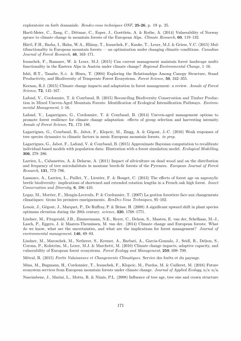
exploratoire en forêt domaniale. Rendez-vous techniques ONF, 25-26, p. 19–p. 25.
Hartl-Meier, C., Zang, C., Dittmar, C., Esper, J., Goettlein, A. & Rothe, A. (2014) Vulnerability of Norwayspruce to climate change in mountain forests of the European Alps. Climate Research, 60, 119–132.
Härtl, F.H., Barka, I., Hahn, W.A., Hlásny, T., Irauschek, F., Knoke, T., Lexer, M.J. & Griess, V.C. (2015) Mul-tifunctionality in European mountain forests — an optimization under changing climatic conditions. CanadianJournal of Forest Research, 46, 163–171.
Irauschek, F., Rammer, W. & Lexer, M.J. (2015) Can current management maintain forest landscape multi-functionality in the Eastern Alps in Austria under climate change? Regional Environmental Change, 1–16.
Ishii, H.T., Tanabe, S.-i. & Hiura, T. (2004) Exploring the Relationships Among Canopy Structure, StandProductivity, and Biodiversity of Temperate Forest Ecosystems. Forest Science, 50, 342–355.
Keenan, R.J. (2015) Climate change impacts and adaptation in forest management: a review. Annals of ForestScience, 72, 145–167.
Lafond, V., Cordonnier, T. & Courbaud, B. (2015) Reconciling Biodiversity Conservation and Timber Produc-tion in Mixed Uneven-Aged Mountain Forests: Identiication of Ecological Intensiication Pathways. Environ-mental Management, 1–16.
Lafond, V., Lagarrigues, G., Cordonnier, T. & Courbaud, B. (2014) Uneven-aged management options topromote forest resilience for climate change adaptation: efects of group selection and harvesting intensity.Annals of Forest Science, 71, 173–186.
Lagarrigues, G., Courbaud, B., Jabot, F., Klopcic, M., Zingg, A. & Gégout, J.-C. (2016) Weak responses oftree species dynamics to climatic factors in mesic European mountain forests. in prep.
Lagarrigues, G., Jabot, F., Lafond, V. & Courbaud, B. (2015) Approximate Bayesian computation to recalibrateindividual-based models with population data: Illustration with a forest simulation model. Ecological Modelling,306, 278–286.
Larrieu, L., Cabanettes, A. & Delarue, A. (2011) Impact of silviculture on dead wood and on the distributionand frequency of tree microhabitats in montane beech-ir forests of the Pyrenees. European Journal of ForestResearch, 131, 773–786.
Lassauce, A., Larrieu, L., Paillet, Y., Lieutier, F. & Bouget, C. (2013) The efects of forest age on saproxylicbeetle biodiversity: implications of shortened and extended rotation lengths in a French oak high forest. InsectConservation and Diversity, 6, 396–410.
Legay, M., Mortier, F., Mengin-Lecreulx, P. & Cordonnier, T. (2007) La gestion forestiere face aux changementsclimatiques: tirons les premiers enseignements. RenDez-Vous Techniques, 95–102.
Lenoir, J., Gégout, J., Marquet, P., De Rufray, P. & Brisse, H. (2008) A signiicant upward shift in plant speciesoptimum elevation during the 20th century. science, 320, 1768–1771.
Lindner, M., Fitzgerald, J.B., Zimmermann, N.E., Reyer, C., Delzon, S., Maaten, E. van der, Schelhaas, M.-J.,Lasch, P., Eggers, J. & Maaten-Theunissen, M. van der. (2014) Climate change and European forests: Whatdo we know, what are the uncertainties, and what are the implications for forest management? Journal ofenvironmental management, 146, 69–83.
Lindner, M., Maroschek, M., Netherer, S., Kremer, A., Barbati, A., Garcia-Gonzalo, J., Seidl, R., Delzon, S.,Corona, P., Kolström, M., Lexer, M.J. & Marchetti, M. (2010) Climate change impacts, adaptive capacity, andvulnerability of European forest ecosystems. Forest Ecology and Management, 259, 698–709.
Métral, R. (2015) Forêts Valaisannes et Changements Climatiques. Service des forêts et du paysage.
Mina, M., Bugmann, H., Cordonnier, T., Irauschek, F., Klopcic, M., Pardos, M. & Cailleret, M. (2016) Futureecosystem services from European mountain forests under climate change. Journal of Applied Ecology, n/a–n/a.
Nascimbene, J., Marini, L., Motta, R. & Nimis, P.L. (2008) Inluence of tree age, tree size and crown structure
171
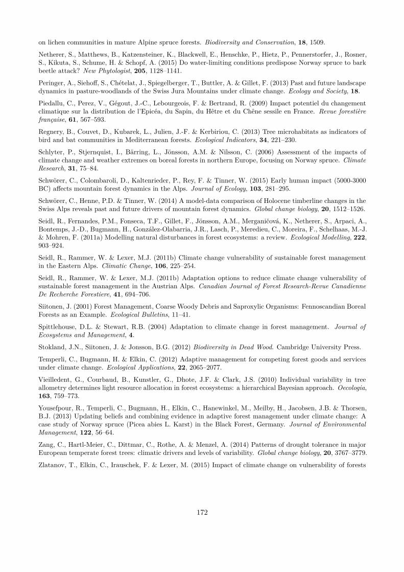
on lichen communities in mature Alpine spruce forests. Biodiversity and Conservation, 18, 1509.
Netherer, S., Matthews, B., Katzensteiner, K., Blackwell, E., Henschke, P., Hietz, P., Pennerstorfer, J., Rosner,S., Kikuta, S., Schume, H. & Schopf, A. (2015) Do water-limiting conditions predispose Norway spruce to barkbeetle attack? New Phytologist, 205, 1128–1141.
Peringer, A., Siehof, S., Chételat, J., Spiegelberger, T., Buttler, A. & Gillet, F. (2013) Past and future landscapedynamics in pasture-woodlands of the Swiss Jura Mountains under climate change. Ecology and Society, 18.
Piedallu, C., Perez, V., Gégout, J.-C., Lebourgeois, F. & Bertrand, R. (2009) Impact potentiel du changementclimatique sur la distribution de l’Epicéa, du Sapin, du Hêtre et du Chêne sessile en France. Revue forestièrefrançaise, 61, 567–593.
Regnery, B., Couvet, D., Kubarek, L., Julien, J.-F. & Kerbiriou, C. (2013) Tree microhabitats as indicators ofbird and bat communities in Mediterranean forests. Ecological Indicators, 34, 221–230.
Schlyter, P., Stjernquist, I., Bärring, L., Jönsson, A.M. & Nilsson, C. (2006) Assessment of the impacts ofclimate change and weather extremes on boreal forests in northern Europe, focusing on Norway spruce. ClimateResearch, 31, 75–84.
Schwörer, C., Colombaroli, D., Kaltenrieder, P., Rey, F. & Tinner, W. (2015) Early human impact (5000-3000BC) afects mountain forest dynamics in the Alps. Journal of Ecology, 103, 281–295.
Schwörer, C., Henne, P.D. & Tinner, W. (2014) A model-data comparison of Holocene timberline changes in theSwiss Alps reveals past and future drivers of mountain forest dynamics. Global change biology, 20, 1512–1526.
Seidl, R., Fernandes, P.M., Fonseca, T.F., Gillet, F., Jönsson, A.M., Merganičová, K., Netherer, S., Arpaci, A.,Bontemps, J.-D., Bugmann, H., González-Olabarria, J.R., Lasch, P., Meredieu, C., Moreira, F., Schelhaas, M.-J.& Mohren, F. (2011a) Modelling natural disturbances in forest ecosystems: a review. Ecological Modelling, 222,903–924.
Seidl, R., Rammer, W. & Lexer, M.J. (2011b) Climate change vulnerability of sustainable forest managementin the Eastern Alps. Climatic Change, 106, 225–254.
Seidl, R., Rammer, W. & Lexer, M.J. (2011b) Adaptation options to reduce climate change vulnerability ofsustainable forest management in the Austrian Alps. Canadian Journal of Forest Research-Revue CanadienneDe Recherche Forestiere, 41, 694–706.
Siitonen, J. (2001) Forest Management, Coarse Woody Debris and Saproxylic Organisms: Fennoscandian BorealForests as an Example. Ecological Bulletins, 11–41.
Spittlehouse, D.L. & Stewart, R.B. (2004) Adaptation to climate change in forest management. Journal ofEcosystems and Management, 4.
Stokland, J.N., Siitonen, J. & Jonsson, B.G. (2012) Biodiversity in Dead Wood. Cambridge University Press.
Temperli, C., Bugmann, H. & Elkin, C. (2012) Adaptive management for competing forest goods and servicesunder climate change. Ecological Applications, 22, 2065–2077.
Vieilledent, G., Courbaud, B., Kunstler, G., Dhote, J.F. & Clark, J.S. (2010) Individual variability in treeallometry determines light resource allocation in forest ecosystems: a hierarchical Bayesian approach. Oecologia,163, 759–773.
Yousefpour, R., Temperli, C., Bugmann, H., Elkin, C., Hanewinkel, M., Meilby, H., Jacobsen, J.B. & Thorsen,B.J. (2013) Updating beliefs and combining evidence in adaptive forest management under climate change: Acase study of Norway spruce (Picea abies L. Karst) in the Black Forest, Germany. Journal of EnvironmentalManagement, 122, 56–64.
Zang, C., Hartl-Meier, C., Dittmar, C., Rothe, A. & Menzel, A. (2014) Patterns of drought tolerance in majorEuropean temperate forest trees: climatic drivers and levels of variability. Global change biology, 20, 3767–3779.
Zlatanov, T., Elkin, C., Irauschek, F. & Lexer, M. (2015) Impact of climate change on vulnerability of forests
172

and ecosystem service supply in Western Rhodopes Mountains. Regional Environmental Change, 1–13.
173

Supplementary information for manuscript ‘Stand-level managementoptions to preserve goods and services provided by uneven-aged moun-tain forests in a context of climate change’
Guillaume Lagarrigues, Franck Jabot, Sylvain Dupire, Benoît Courbaud
174
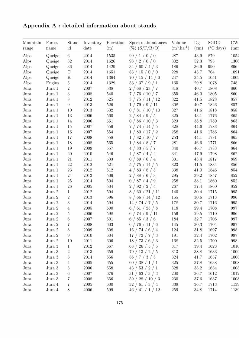
Appendix A : detailed information about stands
Mountainrange
Forestname
Standid
Inventorydate
Elevation(m)
Species abundances(%) (S/F/B/O)
Volume(m3.ha-1)
Dg(cm)
SGDD(°C.days)
CWB(mm)
Alps Queige 6 2014 1535 99 / 1 / 0 / 0 287 43.9 879 1054Alps Queige 32 2014 1626 98 / 2 / 0 / 0 302 52.3 795 1306Alps Queige 36 2014 1429 34 / 60 / 4 / 3 186 36.9 990 896Alps Queige C 2014 1651 85 / 15 / 0 / 0 228 43.7 764 1091Alps Queige K 2014 1364 70 / 15 / 14 / 0 247 35.5 1051 1009Alps Engins 5 2014 1329 53 / 37 / 9 / 1 165 29.8 1078 748Jura Jura 1 2 2007 538 2 / 68 / 23 / 7 318 40.7 1808 860Jura Jura 1 3 2008 540 7 / 76 / 10 / 7 355 46.0 1805 860Jura Jura 1 8 2012 525 3 / 75 / 11 / 12 322 41.5 1828 857Jura Jura 1 9 2013 526 1 / 79 / 9 / 11 308 40.7 1826 857Jura Jura 1 10 2013 532 0 / 81 / 10 / 10 327 41.6 1818 858Jura Jura 1 13 2006 560 2 / 84 / 9 / 5 325 43.1 1776 865Jura Jura 1 14 2006 551 0 / 86 / 10 / 3 323 38.8 1789 863Jura Jura 1 15 2007 556 7 / 74 / 14 / 5 328 44.6 1783 864Jura Jura 1 16 2007 554 1 / 80 / 17 / 2 258 41.6 1786 864Jura Jura 1 17 2008 558 1 / 82 / 10 / 7 253 44.1 1781 865Jura Jura 1 18 2008 565 1 / 84 / 8 / 7 281 46.6 1771 866Jura Jura 1 19 2009 557 4 / 83 / 5 / 7 340 46.7 1783 864Jura Jura 1 20 2010 546 4 / 87 / 4 / 4 341 47.9 1798 862Jura Jura 1 21 2011 533 0 / 89 / 6 / 4 331 43.4 1817 859Jura Jura 1 22 2012 521 5 / 75 / 14 / 5 323 41.5 1834 856Jura Jura 1 23 2012 512 4 / 83 / 8 / 5 338 41.0 1846 854Jura Jura 1 24 2013 506 2 / 88 / 6 / 3 295 39.2 1857 852Jura Jura 1 25 2014 504 0 / 87 / 4 / 9 258 38.1 1860 852Jura Jura 1 26 2005 504 2 / 92 / 2 / 4 267 37.4 1860 852Jura Jura 2 1 2012 594 8 / 60 / 21 / 11 140 30.4 1715 995Jura Jura 2 2 2013 596 8 / 66 / 14 / 12 155 30.6 1713 996Jura Jura 2 3 2014 594 14 / 74 / 7 / 5 178 30.7 1716 995Jura Jura 2 4 2005 600 6 / 61 / 25 / 8 118 29.4 1708 997Jura Jura 2 5 2006 598 6 / 74 / 9 / 11 156 29.5 1710 996Jura Jura 2 6 2007 601 6 / 85 / 3 / 6 184 32.7 1706 997Jura Jura 2 7 2008 603 6 / 76 / 11 / 6 145 30.3 1704 997Jura Jura 2 8 2009 608 16 / 74 / 6 / 4 124 31.8 1697 998Jura Jura 2 9 2010 604 17 / 72 / 7 / 3 191 32.4 1702 997Jura Jura 2 10 2011 606 18 / 73 / 6 / 3 168 32.5 1700 998Jura Jura 3 1 2012 667 63 / 26 / 5 / 5 317 39.4 1623 1010Jura Jura 3 2 2013 659 79 / 13 / 2 / 5 313 38.8 1633 1009Jura Jura 3 3 2014 656 86 / 7 / 3 / 5 324 41.7 1637 1008Jura Jura 3 4 2005 655 60 / 38 / 1 / 1 325 37.8 1638 1008Jura Jura 3 5 2006 658 43 / 53 / 2 / 1 328 38.2 1634 1008Jura Jura 3 6 2007 676 31 / 63 / 3 / 3 200 36.7 1612 1012Jura Jura 3 7 2008 656 59 / 28 / 10 / 3 230 37.6 1637 1008Jura Jura 4 7 2005 600 32 / 61 / 3 / 4 339 36.7 1713 1139Jura Jura 4 8 2006 599 46 / 41 / 1 / 12 259 34.8 1714 1139
175
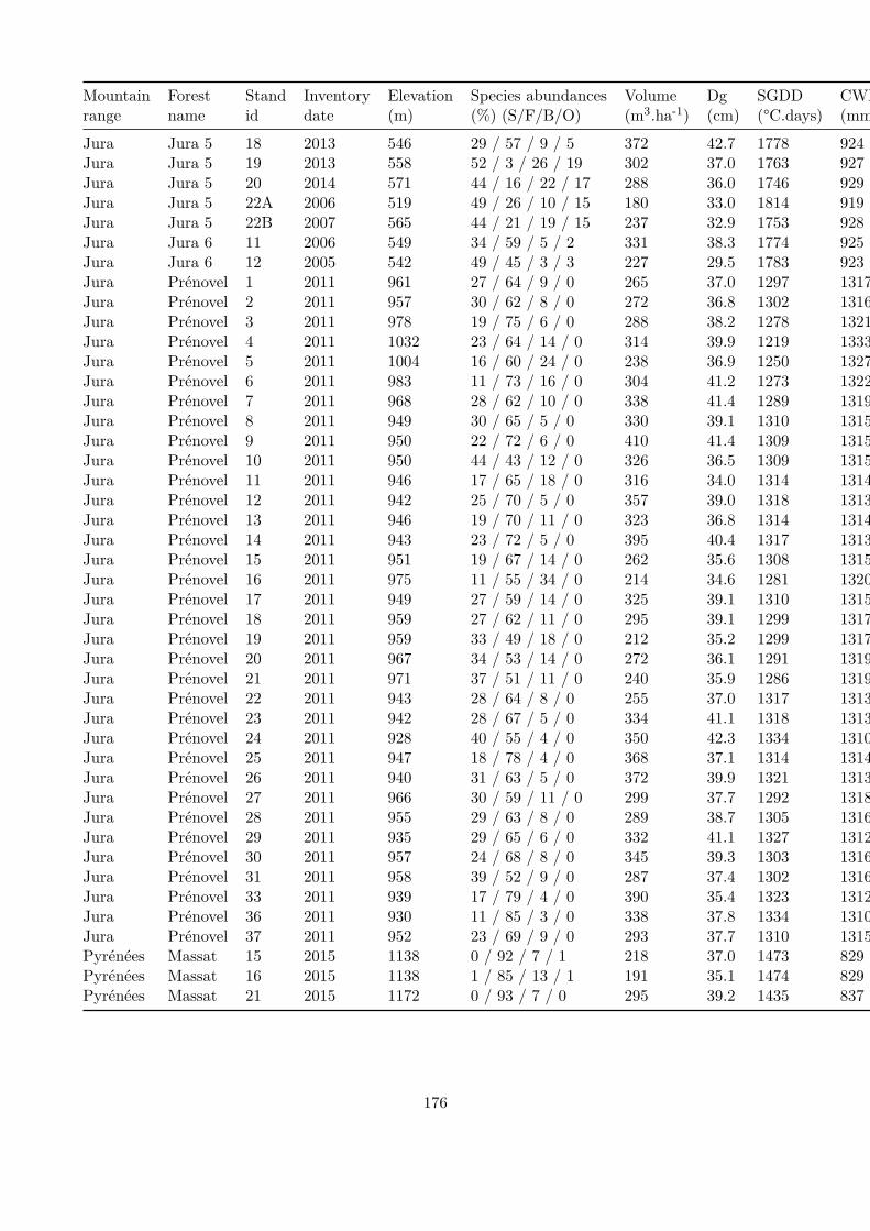
Mountainrange
Forestname
Standid
Inventorydate
Elevation(m)
Species abundances(%) (S/F/B/O)
Volume(m3.ha-1)
Dg(cm)
SGDD(°C.days)
CWB(mm)
Jura Jura 5 18 2013 546 29 / 57 / 9 / 5 372 42.7 1778 924Jura Jura 5 19 2013 558 52 / 3 / 26 / 19 302 37.0 1763 927Jura Jura 5 20 2014 571 44 / 16 / 22 / 17 288 36.0 1746 929Jura Jura 5 22A 2006 519 49 / 26 / 10 / 15 180 33.0 1814 919Jura Jura 5 22B 2007 565 44 / 21 / 19 / 15 237 32.9 1753 928Jura Jura 6 11 2006 549 34 / 59 / 5 / 2 331 38.3 1774 925Jura Jura 6 12 2005 542 49 / 45 / 3 / 3 227 29.5 1783 923Jura Prénovel 1 2011 961 27 / 64 / 9 / 0 265 37.0 1297 1317Jura Prénovel 2 2011 957 30 / 62 / 8 / 0 272 36.8 1302 1316Jura Prénovel 3 2011 978 19 / 75 / 6 / 0 288 38.2 1278 1321Jura Prénovel 4 2011 1032 23 / 64 / 14 / 0 314 39.9 1219 1333Jura Prénovel 5 2011 1004 16 / 60 / 24 / 0 238 36.9 1250 1327Jura Prénovel 6 2011 983 11 / 73 / 16 / 0 304 41.2 1273 1322Jura Prénovel 7 2011 968 28 / 62 / 10 / 0 338 41.4 1289 1319Jura Prénovel 8 2011 949 30 / 65 / 5 / 0 330 39.1 1310 1315Jura Prénovel 9 2011 950 22 / 72 / 6 / 0 410 41.4 1309 1315Jura Prénovel 10 2011 950 44 / 43 / 12 / 0 326 36.5 1309 1315Jura Prénovel 11 2011 946 17 / 65 / 18 / 0 316 34.0 1314 1314Jura Prénovel 12 2011 942 25 / 70 / 5 / 0 357 39.0 1318 1313Jura Prénovel 13 2011 946 19 / 70 / 11 / 0 323 36.8 1314 1314Jura Prénovel 14 2011 943 23 / 72 / 5 / 0 395 40.4 1317 1313Jura Prénovel 15 2011 951 19 / 67 / 14 / 0 262 35.6 1308 1315Jura Prénovel 16 2011 975 11 / 55 / 34 / 0 214 34.6 1281 1320Jura Prénovel 17 2011 949 27 / 59 / 14 / 0 325 39.1 1310 1315Jura Prénovel 18 2011 959 27 / 62 / 11 / 0 295 39.1 1299 1317Jura Prénovel 19 2011 959 33 / 49 / 18 / 0 212 35.2 1299 1317Jura Prénovel 20 2011 967 34 / 53 / 14 / 0 272 36.1 1291 1319Jura Prénovel 21 2011 971 37 / 51 / 11 / 0 240 35.9 1286 1319Jura Prénovel 22 2011 943 28 / 64 / 8 / 0 255 37.0 1317 1313Jura Prénovel 23 2011 942 28 / 67 / 5 / 0 334 41.1 1318 1313Jura Prénovel 24 2011 928 40 / 55 / 4 / 0 350 42.3 1334 1310Jura Prénovel 25 2011 947 18 / 78 / 4 / 0 368 37.1 1314 1314Jura Prénovel 26 2011 940 31 / 63 / 5 / 0 372 39.9 1321 1313Jura Prénovel 27 2011 966 30 / 59 / 11 / 0 299 37.7 1292 1318Jura Prénovel 28 2011 955 29 / 63 / 8 / 0 289 38.7 1305 1316Jura Prénovel 29 2011 935 29 / 65 / 6 / 0 332 41.1 1327 1312Jura Prénovel 30 2011 957 24 / 68 / 8 / 0 345 39.3 1303 1316Jura Prénovel 31 2011 958 39 / 52 / 9 / 0 287 37.4 1302 1316Jura Prénovel 33 2011 939 17 / 79 / 4 / 0 390 35.4 1323 1312Jura Prénovel 36 2011 930 11 / 85 / 3 / 0 338 37.8 1334 1310Jura Prénovel 37 2011 952 23 / 69 / 9 / 0 293 37.7 1310 1315Pyrénées Massat 15 2015 1138 0 / 92 / 7 / 1 218 37.0 1473 829Pyrénées Massat 16 2015 1138 1 / 85 / 13 / 1 191 35.1 1474 829Pyrénées Massat 21 2015 1172 0 / 93 / 7 / 0 295 39.2 1435 837
176
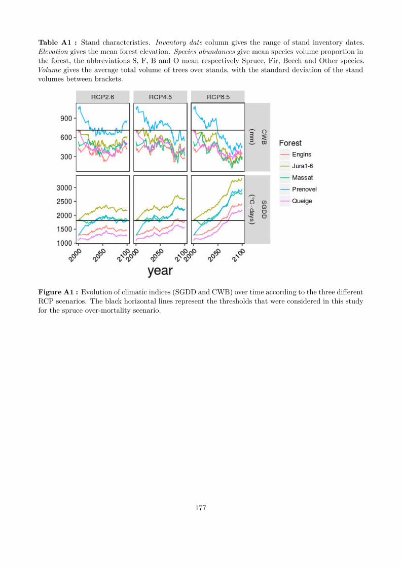
Table A1 : Stand characteristics. Inventory date column gives the range of stand inventory dates.Elevation gives the mean forest elevation. Species abundances give mean species volume proportion inthe forest, the abbreviations S, F, B and O mean respectively Spruce, Fir, Beech and Other species.Volume gives the average total volume of trees over stands, with the standard deviation of the standvolumes between brackets.
Figure A1 : Evolution of climatic indices (SGDD and CWB) over time according to the three diferentRCP scenarios. The black horizontal lines represent the thresholds that were considered in this studyfor the spruce over-mortality scenario.
177
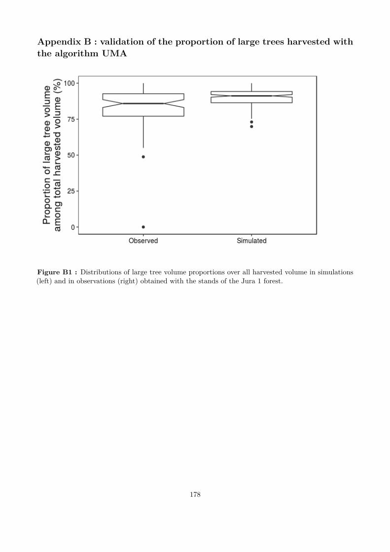
Appendix B : validation of the proportion of large trees harvested withthe algorithm UMA
Figure B1 : Distributions of large tree volume proportions over all harvested volume in simulations(left) and in observations (right) obtained with the stands of the Jura 1 forest.
178
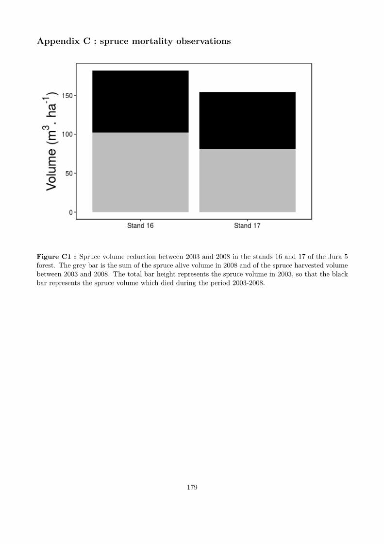
Appendix C : spruce mortality observations
Figure C1 : Spruce volume reduction between 2003 and 2008 in the stands 16 and 17 of the Jura 5forest. The grey bar is the sum of the spruce alive volume in 2008 and of the spruce harvested volumebetween 2003 and 2008. The total bar height represents the spruce volume in 2003, so that the blackbar represents the spruce volume which died during the period 2003-2008.
179
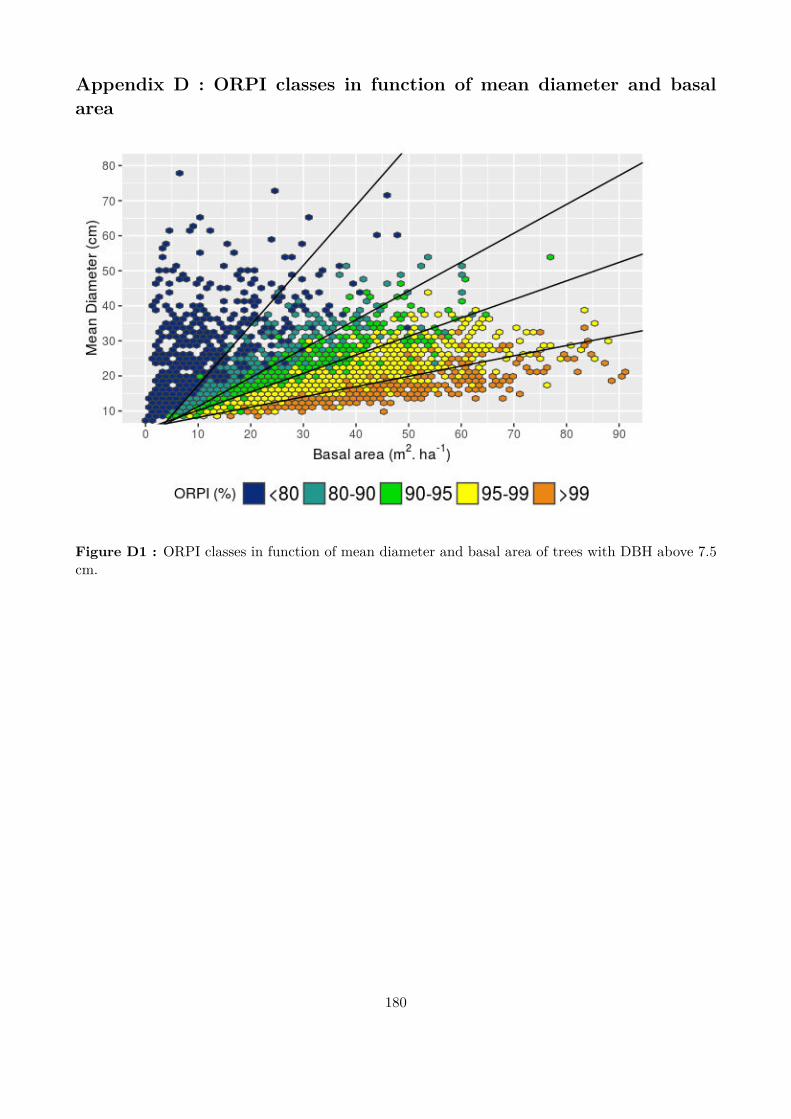
Appendix D : ORPI classes in function of mean diameter and basalarea
Figure D1 : ORPI classes in function of mean diameter and basal area of trees with DBH above 7.5cm.
180
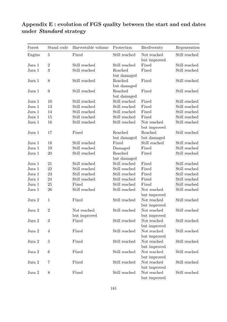
Appendix E : evolution of FGS quality between the start and end datesunder Standard strategy
Forest Stand code Harvestable volume Protection Biodiversity RegenerationEngins 5 Fixed Still reached Not reached
but improvedStill reached
Jura 1 2 Still reached Still reached Fixed Still reachedJura 1 3 Still reached Reached
but damagedFixed Still reached
Jura 1 8 Still reached Reachedbut damaged
Fixed Still reached
Jura 1 9 Still reached Reachedbut damaged
Fixed Still reached
Jura 1 10 Still reached Still reached Fixed Still reachedJura 1 13 Still reached Still reached Fixed Still reachedJura 1 14 Still reached Still reached Fixed Still reachedJura 1 15 Still reached Still reached Fixed Still reachedJura 1 16 Still reached Still reached Not reached
but improvedStill reached
Jura 1 17 Fixed Reachedbut damaged
Reachedbut damaged
Still reached
Jura 1 18 Still reached Fixed Still reached Still reachedJura 1 19 Still reached Damaged Fixed Still reachedJura 1 20 Still reached Reached
but damagedFixed Still reached
Jura 1 21 Still reached Still reached Fixed Still reachedJura 1 22 Still reached Still reached Fixed Still reachedJura 1 23 Still reached Still reached Fixed Still reachedJura 1 24 Still reached Still reached Fixed Still reachedJura 1 25 Fixed Still reached Fixed Still reachedJura 1 26 Still reached Still reached Not reached
but improvedStill reached
Jura 2 1 Fixed Still reached Not reachedbut improved
Still reached
Jura 2 2 Not reachedbut improved
Still reached Not reachedbut improved
Still reached
Jura 2 3 Fixed Still reached Not reachedbut improved
Still reached
Jura 2 4 Fixed Still reached Not reachedbut improved
Still reached
Jura 2 5 Fixed Still reached Not reachedbut improved
Still reached
Jura 2 6 Fixed Still reached Not reachedbut improved
Still reached
Jura 2 7 Fixed Still reached Not reachedbut improved
Still reached
Jura 2 8 Fixed Still reached Not reachedbut improved
Still reached
181
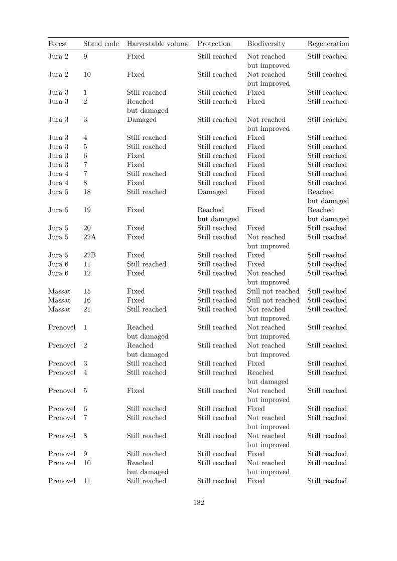
Forest Stand code Harvestable volume Protection Biodiversity RegenerationJura 2 9 Fixed Still reached Not reached
but improvedStill reached
Jura 2 10 Fixed Still reached Not reachedbut improved
Still reached
Jura 3 1 Still reached Still reached Fixed Still reachedJura 3 2 Reached
but damagedStill reached Fixed Still reached
Jura 3 3 Damaged Still reached Not reachedbut improved
Still reached
Jura 3 4 Still reached Still reached Fixed Still reachedJura 3 5 Still reached Still reached Fixed Still reachedJura 3 6 Fixed Still reached Fixed Still reachedJura 3 7 Fixed Still reached Fixed Still reachedJura 4 7 Still reached Still reached Fixed Still reachedJura 4 8 Fixed Still reached Fixed Still reachedJura 5 18 Still reached Damaged Fixed Reached
but damagedJura 5 19 Fixed Reached
but damagedFixed Reached
but damagedJura 5 20 Fixed Still reached Fixed Still reachedJura 5 22A Fixed Still reached Not reached
but improvedStill reached
Jura 5 22B Fixed Still reached Fixed Still reachedJura 6 11 Still reached Still reached Fixed Still reachedJura 6 12 Fixed Still reached Not reached
but improvedStill reached
Massat 15 Fixed Still reached Still not reached Still reachedMassat 16 Fixed Still reached Still not reached Still reachedMassat 21 Still reached Still reached Not reached
but improvedStill reached
Prenovel 1 Reachedbut damaged
Still reached Not reachedbut improved
Still reached
Prenovel 2 Reachedbut damaged
Still reached Not reachedbut improved
Still reached
Prenovel 3 Still reached Still reached Fixed Still reachedPrenovel 4 Still reached Still reached Reached
but damagedStill reached
Prenovel 5 Fixed Still reached Not reachedbut improved
Still reached
Prenovel 6 Still reached Still reached Fixed Still reachedPrenovel 7 Still reached Still reached Not reached
but improvedStill reached
Prenovel 8 Still reached Still reached Not reachedbut improved
Still reached
Prenovel 9 Still reached Still reached Fixed Still reachedPrenovel 10 Reached
but damagedStill reached Not reached
but improvedStill reached
Prenovel 11 Still reached Still reached Fixed Still reached
182
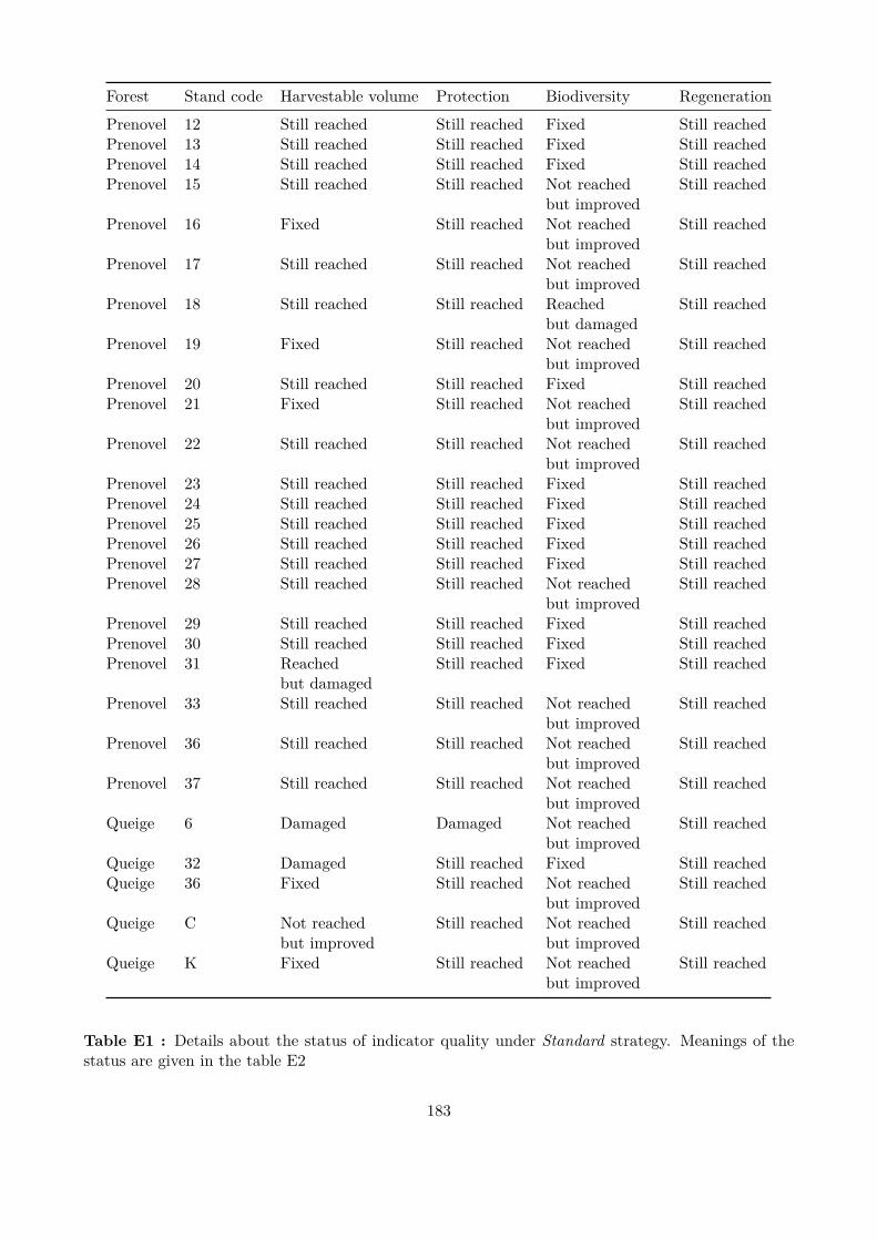
Forest Stand code Harvestable volume Protection Biodiversity RegenerationPrenovel 12 Still reached Still reached Fixed Still reachedPrenovel 13 Still reached Still reached Fixed Still reachedPrenovel 14 Still reached Still reached Fixed Still reachedPrenovel 15 Still reached Still reached Not reached
but improvedStill reached
Prenovel 16 Fixed Still reached Not reachedbut improved
Still reached
Prenovel 17 Still reached Still reached Not reachedbut improved
Still reached
Prenovel 18 Still reached Still reached Reachedbut damaged
Still reached
Prenovel 19 Fixed Still reached Not reachedbut improved
Still reached
Prenovel 20 Still reached Still reached Fixed Still reachedPrenovel 21 Fixed Still reached Not reached
but improvedStill reached
Prenovel 22 Still reached Still reached Not reachedbut improved
Still reached
Prenovel 23 Still reached Still reached Fixed Still reachedPrenovel 24 Still reached Still reached Fixed Still reachedPrenovel 25 Still reached Still reached Fixed Still reachedPrenovel 26 Still reached Still reached Fixed Still reachedPrenovel 27 Still reached Still reached Fixed Still reachedPrenovel 28 Still reached Still reached Not reached
but improvedStill reached
Prenovel 29 Still reached Still reached Fixed Still reachedPrenovel 30 Still reached Still reached Fixed Still reachedPrenovel 31 Reached
but damagedStill reached Fixed Still reached
Prenovel 33 Still reached Still reached Not reachedbut improved
Still reached
Prenovel 36 Still reached Still reached Not reachedbut improved
Still reached
Prenovel 37 Still reached Still reached Not reachedbut improved
Still reached
Queige 6 Damaged Damaged Not reachedbut improved
Still reached
Queige 32 Damaged Still reached Fixed Still reachedQueige 36 Fixed Still reached Not reached
but improvedStill reached
Queige C Not reachedbut improved
Still reached Not reachedbut improved
Still reached
Queige K Fixed Still reached Not reachedbut improved
Still reached
Table E1 : Details about the status of indicator quality under Standard strategy. Meanings of thestatus are given in the table E2
183
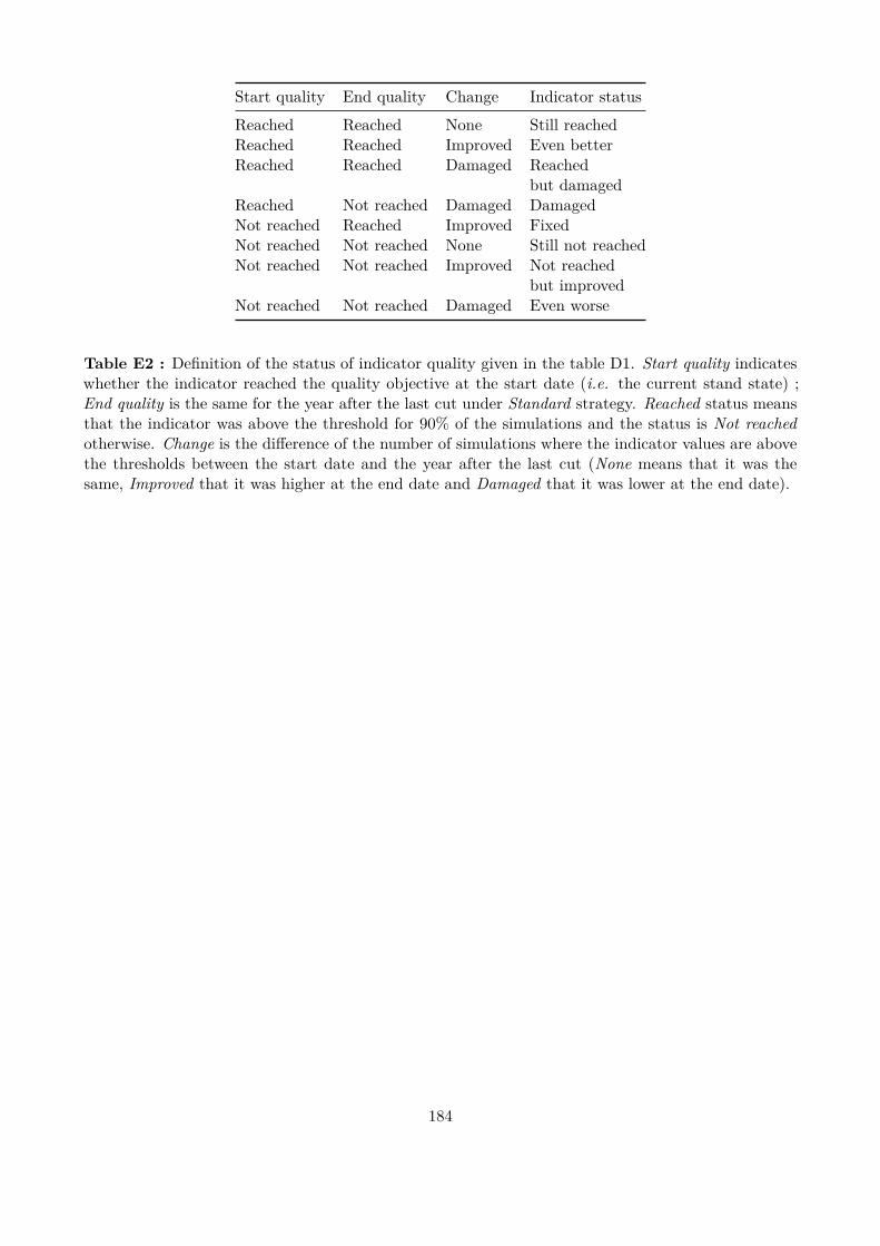
Start quality End quality Change Indicator statusReached Reached None Still reachedReached Reached Improved Even betterReached Reached Damaged Reached
but damagedReached Not reached Damaged DamagedNot reached Reached Improved FixedNot reached Not reached None Still not reachedNot reached Not reached Improved Not reached
but improvedNot reached Not reached Damaged Even worse
Table E2 : Deinition of the status of indicator quality given in the table D1. Start quality indicateswhether the indicator reached the quality objective at the start date (i.e. the current stand state) ;End quality is the same for the year after the last cut under Standard strategy. Reached status meansthat the indicator was above the threshold for 90% of the simulations and the status is Not reachedotherwise. Change is the diference of the number of simulations where the indicator values are abovethe thresholds between the start date and the year after the last cut (None means that it was thesame, Improved that it was higher at the end date and Damaged that it was lower at the end date).
184
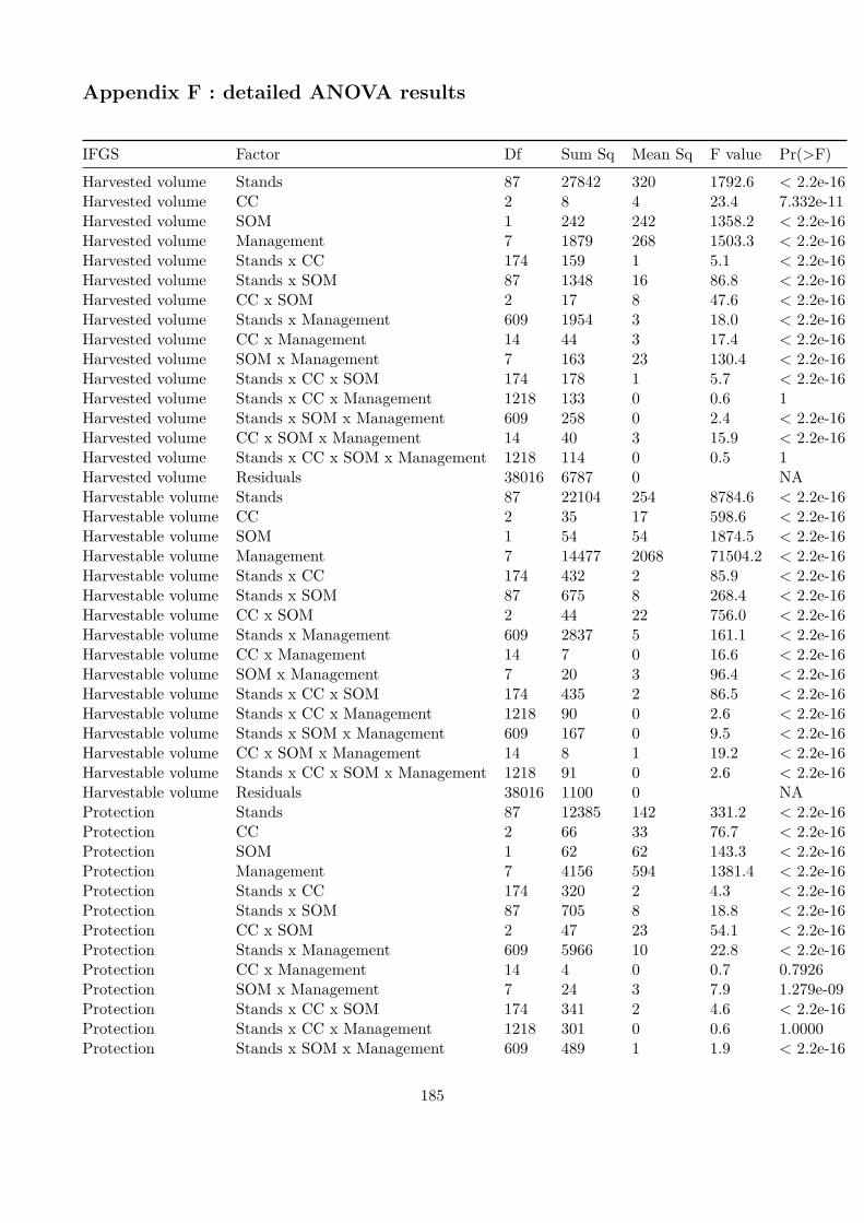
Appendix F : detailed ANOVA results
IFGS Factor Df Sum Sq Mean Sq F value Pr(>F)Harvested volume Stands 87 27842 320 1792.6 < 2.2e-16Harvested volume CC 2 8 4 23.4 7.332e-11Harvested volume SOM 1 242 242 1358.2 < 2.2e-16Harvested volume Management 7 1879 268 1503.3 < 2.2e-16Harvested volume Stands x CC 174 159 1 5.1 < 2.2e-16Harvested volume Stands x SOM 87 1348 16 86.8 < 2.2e-16Harvested volume CC x SOM 2 17 8 47.6 < 2.2e-16Harvested volume Stands x Management 609 1954 3 18.0 < 2.2e-16Harvested volume CC x Management 14 44 3 17.4 < 2.2e-16Harvested volume SOM x Management 7 163 23 130.4 < 2.2e-16Harvested volume Stands x CC x SOM 174 178 1 5.7 < 2.2e-16Harvested volume Stands x CC x Management 1218 133 0 0.6 1Harvested volume Stands x SOM x Management 609 258 0 2.4 < 2.2e-16Harvested volume CC x SOM x Management 14 40 3 15.9 < 2.2e-16Harvested volume Stands x CC x SOM x Management 1218 114 0 0.5 1Harvested volume Residuals 38016 6787 0 NAHarvestable volume Stands 87 22104 254 8784.6 < 2.2e-16Harvestable volume CC 2 35 17 598.6 < 2.2e-16Harvestable volume SOM 1 54 54 1874.5 < 2.2e-16Harvestable volume Management 7 14477 2068 71504.2 < 2.2e-16Harvestable volume Stands x CC 174 432 2 85.9 < 2.2e-16Harvestable volume Stands x SOM 87 675 8 268.4 < 2.2e-16Harvestable volume CC x SOM 2 44 22 756.0 < 2.2e-16Harvestable volume Stands x Management 609 2837 5 161.1 < 2.2e-16Harvestable volume CC x Management 14 7 0 16.6 < 2.2e-16Harvestable volume SOM x Management 7 20 3 96.4 < 2.2e-16Harvestable volume Stands x CC x SOM 174 435 2 86.5 < 2.2e-16Harvestable volume Stands x CC x Management 1218 90 0 2.6 < 2.2e-16Harvestable volume Stands x SOM x Management 609 167 0 9.5 < 2.2e-16Harvestable volume CC x SOM x Management 14 8 1 19.2 < 2.2e-16Harvestable volume Stands x CC x SOM x Management 1218 91 0 2.6 < 2.2e-16Harvestable volume Residuals 38016 1100 0 NAProtection Stands 87 12385 142 331.2 < 2.2e-16Protection CC 2 66 33 76.7 < 2.2e-16Protection SOM 1 62 62 143.3 < 2.2e-16Protection Management 7 4156 594 1381.4 < 2.2e-16Protection Stands x CC 174 320 2 4.3 < 2.2e-16Protection Stands x SOM 87 705 8 18.8 < 2.2e-16Protection CC x SOM 2 47 23 54.1 < 2.2e-16Protection Stands x Management 609 5966 10 22.8 < 2.2e-16Protection CC x Management 14 4 0 0.7 0.7926Protection SOM x Management 7 24 3 7.9 1.279e-09Protection Stands x CC x SOM 174 341 2 4.6 < 2.2e-16Protection Stands x CC x Management 1218 301 0 0.6 1.0000Protection Stands x SOM x Management 609 489 1 1.9 < 2.2e-16
185
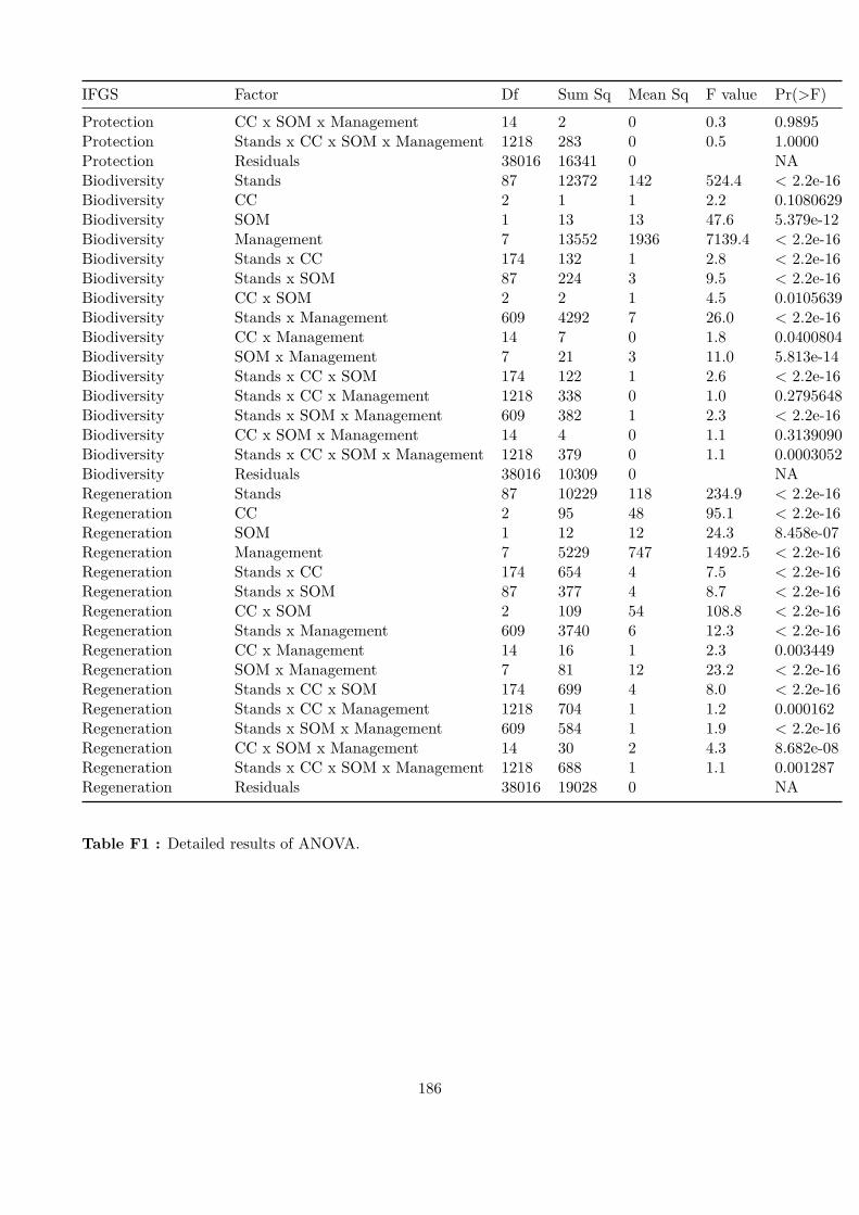
IFGS Factor Df Sum Sq Mean Sq F value Pr(>F)Protection CC x SOM x Management 14 2 0 0.3 0.9895Protection Stands x CC x SOM x Management 1218 283 0 0.5 1.0000Protection Residuals 38016 16341 0 NABiodiversity Stands 87 12372 142 524.4 < 2.2e-16Biodiversity CC 2 1 1 2.2 0.1080629Biodiversity SOM 1 13 13 47.6 5.379e-12Biodiversity Management 7 13552 1936 7139.4 < 2.2e-16Biodiversity Stands x CC 174 132 1 2.8 < 2.2e-16Biodiversity Stands x SOM 87 224 3 9.5 < 2.2e-16Biodiversity CC x SOM 2 2 1 4.5 0.0105639Biodiversity Stands x Management 609 4292 7 26.0 < 2.2e-16Biodiversity CC x Management 14 7 0 1.8 0.0400804Biodiversity SOM x Management 7 21 3 11.0 5.813e-14Biodiversity Stands x CC x SOM 174 122 1 2.6 < 2.2e-16Biodiversity Stands x CC x Management 1218 338 0 1.0 0.2795648Biodiversity Stands x SOM x Management 609 382 1 2.3 < 2.2e-16Biodiversity CC x SOM x Management 14 4 0 1.1 0.3139090Biodiversity Stands x CC x SOM x Management 1218 379 0 1.1 0.0003052Biodiversity Residuals 38016 10309 0 NARegeneration Stands 87 10229 118 234.9 < 2.2e-16Regeneration CC 2 95 48 95.1 < 2.2e-16Regeneration SOM 1 12 12 24.3 8.458e-07Regeneration Management 7 5229 747 1492.5 < 2.2e-16Regeneration Stands x CC 174 654 4 7.5 < 2.2e-16Regeneration Stands x SOM 87 377 4 8.7 < 2.2e-16Regeneration CC x SOM 2 109 54 108.8 < 2.2e-16Regeneration Stands x Management 609 3740 6 12.3 < 2.2e-16Regeneration CC x Management 14 16 1 2.3 0.003449Regeneration SOM x Management 7 81 12 23.2 < 2.2e-16Regeneration Stands x CC x SOM 174 699 4 8.0 < 2.2e-16Regeneration Stands x CC x Management 1218 704 1 1.2 0.000162Regeneration Stands x SOM x Management 609 584 1 1.9 < 2.2e-16Regeneration CC x SOM x Management 14 30 2 4.3 8.682e-08Regeneration Stands x CC x SOM x Management 1218 688 1 1.1 0.001287Regeneration Residuals 38016 19028 0 NA
Table F1 : Detailed results of ANOVA.
186
![UNION EUROPÉENNE : PROSPECTIVE DÉMOGRAPHIQUE [EU-European Union : population prospective]](https://img.pdfslide.net/doc/110x75/63155251511772fe45104bb9/union-europeenne-prospective-demographique-eu-european-union-population-prospective.jpg)


