Visualization of functional count-comparison-based binaural auditory model output

lable at ScienceDirect

Hearing Research 309 (2014) 147e163

Contents lists avai

Hearing Research

journal homepage: www.elsevier .com/locate/heares

Research paper

Visualization of functional count-comparison-based binaural auditorymodel output

Marko Takanen*, Olli Santala, Ville PulkkiDepartment of Signal Processing and Acoustics, Aalto University School of Electrical Engineering, P.O. Box 13000, FI-00076 Aalto, Finland

a r t i c l e i n f o

Article history:Received 17 December 2012Received in revised form11 October 2013Accepted 15 October 2013Available online 25 October 2013

* Corresponding author. Tel.: þ358 504104055.E-mail addresses: [email protected] (M. T

(O. Santala), [email protected] (V. Pulkki).

0378-5955/$ e see front matter � 2013 Elsevier B.V.http://dx.doi.org/10.1016/j.heares.2013.10.004

a b s t r a c t

The count-comparison principle in binaural auditory modeling is based on the assumption that there arenuclei in the mammalian auditory pathway that encode the directional cues in the rate of the output.When this principle is applied, the outputs of the modeled nuclei do not directly result in a topo-graphically organized map of the auditory space that could be monitored as such. Therefore, this articlepresents a method for visualizing the information from the outputs as well as the nucleus models. Thefunctionality of the auditory model presented here is tested in various binaural listening scenarios,including localization tasks and the discrimination of a target in the presence of distracting sound as wellas sound scenarios consisting of multiple simultaneous sound sources. The performance of the model isillustrated with binaural activity maps. The activations seen in the maps are compared to human per-formance in similar scenarios, and it is shown that the performance of the model is in accordance withthe psychoacoustical data.

� 2013 Elsevier B.V. All rights reserved.

1. Introduction

Functional binaural auditory models target to estimate thespatial perception of sound by processing digitized signals(Colburn, 1996). Ideally, the spatial aspects of sound scenes areshown in the output of the model at the same resolution in time,frequency, and space as humans hear them. When successful, suchmodels help to understand the functioning of the binaural auditorypathway, and can also be applied tomany other fields, such as audioquality assessment and robotics (Blauert, 2013).

Such functional binaural auditory models have been researchedactively during the last few decades (for a review, see, e.g., Colburn,1996). An influential model was proposed by Jeffress (1948), whereit is assumed that the nerves at each auditory band from both earsare connected by an array of coincidence detectors. The conductiondelay from the ear to the detectors is assumed to vary in such a waythat the position of the most active detector reveals the left/rightcue of the sound in each frequency band. The outputs of the coin-cidence counters in the model can be seen as a topographicallyorganized set of neurons, where the level of a neuron’s output ishighest when the interaural time difference (ITD) of the incomingsound matches the conduction delay difference in the nerves.The principle is typically implemented with normalized

akanen), [email protected]

All rights reserved.

cross-correlation in auditory filter bands with time lags approxi-mately within the physiologic ITD range, and it is only sensitive toITD. This principle makes it possible to visualize complex soundscenarios with cross-correlograms (Shackleton et al., 1992), whichshow the binaural activity in the left/right dimension as a functionof either frequency or time. Several extensions of the Jeffress modelhave been presented as well (see, e.g., Lindemann,1986; Gaik, 1993;Faller and Merimaa, 2004).

Another principle has been suggested for the decoding of ITDand interaural level differences (ILD), where the nuclei in eachhemisphere are assumed to encode the left/right direction of soundsimply in the rate of the output. The values of each side arecompared together, which gives the name count-comparisonmodel (von Békésy, 1930; von Békésy and Wever, 1960; vanBergeijk et al., 1962). The principle is also called hemifield codingor opponent coding (Salminen et al., 2010; Stecker et al., 2005).Alternatively, Pulkki and Hirvonen (2009) assume that the encod-ing method is self-normalized, whichmeans that the comparison isnot needed and that the output value of the nucleus in the hemi-sphere is already a meaningful directional coordinate. The result isthus a directional cue that can be associated with the corre-sponding temporal position of the auditory band; this differsnotably from the Jeffress modeling principle, where the output canbe seen as a topographic mapping of auditory space.

The neurophysiology and neuroanatomy of the binaural audi-tory pathway has been researched actively as well (see, e.g.,Brugge et al., 1969; Eisenman, 1974; Mäkelä and McEvoy, 1996;

Delta:1_given name

Delta:1_surname

Delta:1_given name

mailto:[email protected]



http://crossmark.crossref.org/dialog/?doi=10.1016/j.heares.2013.10.004&domain=pdf

www.sciencedirect.com/science/journal/03785955

http://www.elsevier.com/locate/heares

http://dx.doi.org/10.1016/j.heares.2013.10.004



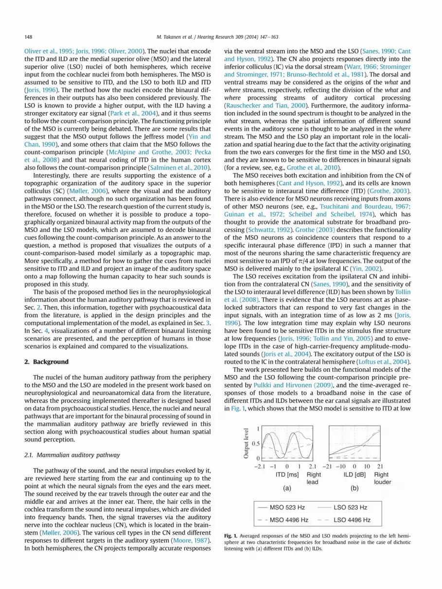
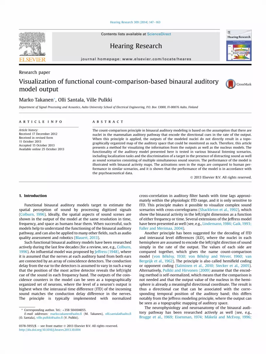
Fig. 1. Averaged responses of the MSO and LSO models projecting to the left hemi-sphere at two characteristic frequencies for broadband noise in the case of dichoticlistening with (a) different ITDs and (b) ILDs.

M. Takanen et al. / Hearing Research 309 (2014) 147e163148

Oliver et al., 1995; Joris, 1996; Oliver, 2000). The nuclei that encodethe ITD and ILD are the medial superior olive (MSO) and the lateralsuperior olive (LSO) nuclei of both hemispheres, which receiveinput from the cochlear nuclei from both hemispheres. The MSO isassumed to be sensitive to ITD, and the LSO to both ILD and ITD(Joris, 1996). The method how the nuclei encode the binaural dif-ferences in their outputs has also been considered previously. TheLSO is known to provide a higher output, with the ILD having astronger excitatory ear signal (Park et al., 2004), and it thus seemsto follow the count-comparison principle. The functioning principleof the MSO is currently being debated. There are some results thatsuggest that the MSO output follows the Jeffress model (Yin andChan, 1990), and some others that claim that the MSO follows thecount-comparison principle (McAlpine and Grothe, 2003; Peckaet al., 2008) and that neural coding of ITD in the human cortexalso follows the count-comparison principle (Salminen et al., 2010).

Interestingly, there are results supporting the existence of atopographic organization of the auditory space in the superiorcolliculus (SC) (Møller, 2006), where the visual and the auditorypathways connect, although no such organization has been foundin theMSO or the LSO. The research question of the current study is,therefore, focused on whether it is possible to produce a topo-graphically organized binaural activity map from the outputs of theMSO and the LSO models, which are assumed to decode binauralcues following the count-comparison principle. As an answer to thequestion, a method is proposed that visualizes the outputs of acount-comparison-based model similarly as a topographic map.More specifically, a method for how to gather the cues from nucleisensitive to ITD and ILD and project an image of the auditory spaceonto a map following the human capacity to hear such sounds isproposed in this study.

The basis of the proposed method lies in the neurophysiologicalinformation about the human auditory pathway that is reviewed inSec. 2. Then, this information, together with psychoacoustical datafrom the literature, is applied in the design principles and thecomputational implementation of the model, as explained in Sec. 3.In Sec. 4, visualizations of a number of different binaural listeningscenarios are presented, and the perception of humans in thosescenarios is explained and compared to the visualizations.

2. Background

The nuclei of the human auditory pathway from the peripheryto the MSO and the LSO are modeled in the present work based onneurophysiological and neuroanatomical data from the literature,whereas the processing implemented thereafter is designed basedon data from psychoacoustical studies. Hence, the nuclei and neuralpathways that are important for the binaural processing of sound inthe mammalian auditory pathway are briefly reviewed in thissection along with psychoacoustical studies about human spatialsound perception.

2.1. Mammalian auditory pathway

The pathway of the sound, and the neural impulses evoked by it,are reviewed here starting from the ear and continuing up to thepoint at which the neural signals from the eyes and the ears meet.The sound received by the ear travels through the outer ear and themiddle ear and arrives at the inner ear. There, the hair cells in thecochlea transform the sound into neural impulses, which are dividedinto frequency bands. Then, the signal traverses via the auditorynerve into the cochlear nucleus (CN), which is located in the brain-stem (Møller, 2006). The various cell types in the CN send differentresponses to different targets in the auditory system (Moore, 1987).In both hemispheres, the CN projects temporally accurate responses

via the ventral stream into the MSO and the LSO (Sanes, 1990; Cantand Hyson, 1992). The CN also projects responses directly into theinferior colliculus (IC) via the dorsal stream (Warr, 1966; Stromingerand Strominger, 1971; Brunso-Bechtold et al., 1981). The dorsal andventral streams may be considered as the origins of the what andwhere streams, respectively, reflecting the division of the what andwhere processing streams of auditory cortical processing(Rauschecker and Tian, 2000). Furthermore, the auditory informa-tion included in the sound spectrum is thought to be analyzed in thewhat stream, whereas the spatial information of different soundevents in the auditory scene is thought to be analyzed in the wherestream. The MSO and the LSO play an important role in the locali-zation and spatial hearing due to the fact that the activity originatingfrom the two ears converges for the first time in the MSO and LSO,and they are known to be sensitive to differences in binaural signals(for a review, see, e.g., Grothe et al., 2010).

The MSO receives both excitation and inhibition from the CN ofboth hemispheres (Cant and Hyson, 1992), and its cells are knownto be sensitive to interaural time difference (ITD) (Grothe, 2003).There is also evidence for MSO neurons receiving inputs from axonsof other MSO neurons (see, e.g., Tsuchitani and Bourdeau, 1967;Guinan et al., 1972; Scheibel and Scheibel, 1974), which hasthought to provide the anatomical substrate for broadband pro-cessing (Schwattz, 1992). Grothe (2003) describes the functionalityof the MSO neurons as coincidence counters that respond to aspecific interaural phase difference (IPD) in such a manner thatmost of the neurons sharing the same characteristic frequency aremost sensitive to an IPD of p/4 at low frequencies. The output of theMSO is delivered mainly to the ipsilateral IC (Yin, 2002).

The LSO receives excitation from the ipsilateral CN and inhibi-tion from the contralateral CN (Sanes, 1990), and the sensitivity ofthe LSO to interaural level difference (ILD) has been shown by Tollinet al. (2008). There is evidence that the LSO neurons act as phase-locked subtractors that can respond to very fast changes in theinput signals, with an integration time of as low as 2 ms (Joris,1996). The low integration time may explain why LSO neuronshave been found to be sensitive ITDs in the stimulus fine structureat low frequencies (Joris, 1996; Tollin and Yin, 2005) and to enve-lope ITDs in the case of high-carrier-frequency amplitude-modu-lated sounds (Joris et al., 2004). The excitatory output of the LSO isrouted to the IC in the contralateral hemisphere (Loftus et al., 2004).

The work presented here builds on the functional models of theMSO and the LSO following the count-comparison principle pre-sented by Pulkki and Hirvonen (2009), and the time-averaged re-sponses of those models to a broadband noise in the case ofdifferent ITDs and ILDs between the ear canal signals are illustratedin Fig. 1, which shows that the MSO model is sensitive to ITD at low

M. Takanen et al. / Hearing Research 309 (2014) 147e163 149

frequencies and that the LSO model is sensitive to ILD at all fre-quencies as well as to ITD at low frequencies.

The role of the IC in binaural processing is still somewhat un-clear, despite the numerous studies that have measured the re-sponses of IC neurons (for a review, see, e.g., Irvine, 1992). This maybe related to the versatility of the IC. What is known of the IC is thatit transmits the spatial information from the CN, MSO, and LSO tothe auditory cortex and the SC, and it may modify the informationin the process (Irvine, 1992).

The superior colliculus (SC) is located next to the IC, and it hasmultiple layers in the nucleus, including layers, for example, forvisual information as well as for sound (Gordon, 1973; Palmer et al.,1982). The SC has been found to be one of the nuclei responsible forcross-modal interaction, and it is also involved in steering the focusof attention towards the stimuli (Stein and Meredith, 1993; Calvert,2001). Interestingly, topographical organization of the auditoryspace has been found in the SC (Palmer et al., 1982; Møller, 2006).The SC includes neurons that respond to multimodal stimulationoriginating from the same spatial location (Gordon, 1973; Peck,1987) and also a map of the auditory space that is aligned withthe visual map in such a manner that the neurons responsive toauditory or visual stimuli from a certain direction can be foundclose to one another (Gordon, 1973; Palmer et al., 1982).

2.2. Psychoacoustical background

The spatial hearing of human listeners has been studied activelyin psychoacoustical experiments over the years (for an extensivereview, see Blauert, 1997). The review presented in this section islimited to the most relevant aspects pertaining to this study.

The sound localization of humans is based on binaural cuesbetween the ear canal signals resulting from differences in the pathof the sound from the sound source to the two ears and on spectralcues caused by the reflections of the sound on the pinna and torso.The binaural cues consist of ITD, ILD, and envelope time-shifts(Blauert, 1997), the last being also referred to as envelope ITD.Typically, the auditory system can use all of the aforementionedcues in the localization process since they all point in the samedirection when a single plane wave arrives at the ears of a listener.However, listening tests conducted in controlled scenarios havedemonstrated that a modification of even one of the binaural dif-ferences (ITD, ILD, IPD, or envelope ITD) away from a zero value issufficient to shift the perceived lateral position of the evokedauditory image away from the center (Lord Rayleigh, 1907; vonBékésy, 1930; Yost, 1981), for example by modifying the stimulusso that only the ITD is non-zero. More specifically, the perceivedlateral position moves towards the side as the ITD is increasedwithin the ITD values that occur in normal situations, that is, thevalues between 0 ms and 0.7 ms that can be caused by the size ofthe human head. With ITD values that exceed those occurring forplane waves, the width of the perceived auditory image changesfrom a point-like image to one with broader extent, while theperceived lateral image remains at the side until the ITD valueexceeds a certain value, after which sound from two different di-rections is perceived. For a broadband noise, the maximum ITD,with which the listeners can still correctly detect the ear beentriggered first, has been shown to vary from three to 10ms betweensubjects (Blodgett et al., 1956). For pure tones, the effects are moreIPD rather than ITD dependent, the limit of correct lateralizationbeing around 170� (Yost, 1981).

The aforementioned tendency of the auditory system to favorthe off-median plane cues in localization is called the lateral pref-erence principle in this article. The experiments on cue trading haveshown that the perceived lateral position of the evoked auditoryimage can be returned back to the center position by introducing

ILD that points to the other side than the ITD that was originallyused to shift the lateral position, or vice versa (David et al., 1959;Harris, 1960; Lang and Buchner, 2008; Dietz et al., 2009). Howev-er, an auditory image that is returned to the center position withconflicting ITD and ILD has been shown to be easily distinguishablefrom a diotic representation (Hafter and Carrier, 1969). In the caseof conflicting non-zero binaural cues, the ITD has been found to bethe dominant cue for both broadband and low-pass filtered stimuli,whereas the ILD has been found to dominate the localization withhigh-pass filtered stimuli (Wightman and Kistler, 1992;Macpherson and Middlebrooks, 2002).

In free-field listening with only one point-like sound source, thesound emitted is perceived as a narrow auditory image (Blauert,1997). The accuracy of the localization in such conditions hasbeen found to depend on the direction of arrival, the type, and thelength of the sound signal (Stevens and Newman, 1936; Boerger,1965; Gardner, 1968). The localization accuracy has often beenmeasured as the minimum audible angle, i.e. the angle the soundsource needs to be shifted from its original direction before thesubject can detect the change. This resolution has been found to beapproximately �1� in front and decrease gradually to approxi-mately�10� when the sound is moved to the side on the horizontalplane (Mills, 1958).

The spatial perception becomes more challenging when thesound heard by the listener actually consists of an ensemble ofindependent signals emitted by multiple sound sources around thelistener. If the task of the listener is to localize a particular soundevent from the ensemble, the ensemble can be thought to consist ofa target sound and distracter(s) that hinder the localization task.Furthermore, the reflections of the target sound in a reverberantenvironment can be considered as distracters as well, and experi-ments on the precedence effect (for a review, see Litovsky et al.,1999) have shown that in such environments, listeners perceivethat the sound is emitted from the direction of the direct sound. Theamount of decrease in the localization of the target sound caused bythe distracter(s) has been found to be dependent on several factors,such as the number of distracters, the signal types, the frequencycontents, the signal-to-noise ratio, and the onset and offset times ofthe target and the distracter(s) (Flanagan and Watson, 1966;Carhart et al., 1969; McFadden and Pasanen, 1976; Kohlrausch,1986; Kollmeier and Gilkey, 1990; Litovsky et al., 1999; Best et al.,2007). Moreover, in conditions that consist of independent noisebursts, the length of the simultaneous noise bursts emitted hasbeen found to have an effect on whether the ensemble is perceivedas point-like or wide (Hirvonen and Pulkki, 2008). Additionally, theperceived width of an ensemble emitting incoherent noise hasbeen found to be slightly narrower than the loudspeaker spanemployed in the reproduction, and that the ends of the distributedensemble are perceived relatively accurately whereas the centerarea is perceived less clearly (Santala and Pulkki, 2011).

If the ensemble consists of multiple speech sources, the scenariois related to the ”cocktail party effect” (Cherry, 1953), where it hasbeen shown that listeners are able to segregate speech in multi-talker situations and are able to both localize the differentspeakers and to identify the sentences spoken by the differentspeakers, although the speech intelligibility and the localizationaccuracy are both worse than in single-source scenarios (Carhartet al., 1969; Bregman, 1994; Hawley et al., 1999).

It should be noted that the overall perception of the auditoryscene is a result of a cognitive process affected not only by theauditory information, but also by the visual information and thehead movements. Support for such an interaction can be found inthe experiments of the ventriloquism (Witkin et al., 1952; Jackson,1953) and the McGurk (McGurk and MacDonald, 1976) effects. Theformer of the mentioned effects demonstrates a shift in the

Fig. 3. Outputs of the cochlea model and the IHC model at two characteristic fre-quencies for a pink noise signal at 60 dB SPL. In this study, the IHC model output to theauditory nerve is used as the output of the periphery model.


localization of a sound towards the visual image of the soundsource, and the latter demonstrates the change in the heard ut-terances caused by conflicting visual and auditory cues. Asmentioned above in Sec. 2.1, the pathways from the eyes and theears meet in the SC. Therefore, the aforementioned effects may beat least partly explained by the processing in the SC.

3. Fundamental model principle and design

The above-mentioned neurophysiological data from the litera-ture about the mammalian auditory pathway and the informationobtained from psychoacoustical experiments have been the basisfor designing the processing steps to form a topographically orga-nized auditory map. The design process is explained in this section,starting from the fundamental principles of the proposed elements.Thereafter, the implementations of those elements are explained indetail.

3.1. Design principle

Since evidence exists of a topographic mapping of the auditoryspace in the SC (see Sec. 2), and since both the what and the whereprocessing streams originating from the CN are known to be con-nected to the IC, all of the information of these streams can beassumed to be available at that level in the forming of such amap. Itis thus suggested in this article to use the where cues to project thewhat cues onto a one-dimensional map representing the left-rightdimension of the auditory space. An analog of this principle is usedin the well-known cathode ray tube, where a number of electronrays are projected onto a fluorescent screen. Different rays producedifferent colors; the brightness of each color depends on the in-tensity of the ray, and the position where the ray hits the screen iscontrolled with the deflection voltage of each color separately.Now, when this principle is applied to a binaural activity map, thewhat cues from the periphery model can be thought of as the raysprojected onto the screen and thewhere cues define the position ofthe rays on the screen. This approach results in a representation ofthe neural activation on a topographically organized map. Morespecifically, the outputs of the MSO, the LSO, and the wide-bandMSO (see Sec. 3.2.4) models are merged together to form one setofwhere cues for each hemisphere; these cues are then used tomapthe what cues originating from the periphery model onto the one-dimensional binaural activity map, as illustrated in Fig. 2. It shouldbe noted that the method is not restricted to combining the outputsof the MSO and the LSO models to form the binaural activity map,as the outputs of either theMSO or LSOmodel are sufficient as such.Additionally, a Jeffress-type MSO model (see, e.g., Colburn

Fig. 2. Structure of the presented model. For simplicity, only the pathw

et al., 1990; Han and Colburn, 1993) can be applied either as suchor in combination with an LSO model, following the count-comparison principle, to provide input signals for the method aswell. A more detailed description of the design principles of thedifferent elements involved in this mapping process is presented inthe following parts of this section.

3.1.1. Cue mergingPsychoacoustical experiments have shown that all sound within

a given critical band can only be perceived as a single sound sourcewith a broader or narrower extent, and that a narrowband binauralstimulus can, in some special cases, be perceived as two distinctauditory objects (Blauert, 1997). However, the present modelprovides three directional cues for each hemisphere, whichcould enable the perception of a narrowband sound in six locations.Such a phenomenon has not been reported in psychoacoustical

ays to the activation projected onto the left hemisphere are shown.


experiments, and therefore, the outputs of the MSO, the LSO, andthe wide-band MSO models on one hemisphere are mergedtogether separately for each CF to form one where cue for thathemisphere. More specifically, the merging is designed to favor thecues pointing more to the side than the ones pointing to the centerin order to emulate the lateral preference principle (see Sec. 2.2). Asa result of this merging, the present model is able to map anarrowband binaural stimulus onto two locations on the binauralactivity map, one on each hemisphere.

3.1.2. Onset weightingThe auditory system is thought to emphasize the onset when

localizing a sound event (Perrot, 1969). For instance, in the exper-iments on the Franssen effect (Franssen, 1960), listeners have beenfound to localize the entire sinusoidal tone to the direction of theonset despite the fact that the majority of the tone was presentedfrom another direction. Later, the effect has been found to exist onlyin non-anechoic conditions (Hartmann and Rakerd,1989). Recently,Dietz et al. (2013) have discovered that lateralization of amplitudemodulated sounds is strongly dominated by the ITDs during themodulation onsets, which also emphasizes the role of modulationonsets in localization of speech and other complex sounds. Thepresent method takes the aforementioned aspects into account byreducing the width of the distribution of the directional cues whena onset is detected and by enhancing the visibility of the onsets onthe binaural activity map.

3.1.3. Topographic mapping of binaural cuesIn this work, the topographic map of the auditory space is

thought to consist of a set of left/right organized neurons in such amanner that there are several frequency-selective neurons in eachposition on the map. Psychoacoustical studies have demonstratedthat the saliency of different cues depends on signals and spatialparameters (Blauert,1997), and that the auditory image evoked by anarrowband stimulus has a point-like, dual, or spread spatial dis-tribution. The basic principle in the proposedmethod is to create animage for each what cue on the activity map. Additionally, thelateral preference principle is taken into account by reducing thestrengths of the images in the hemisphere having images closer tothe midline with a method denoted as contralateral comparison,which effectively amplifies the most lateral activation. Conse-quently, two simultaneous images are created at each frequencyband, one on each hemisphere, when there are conflicting non-zerobinaural cues pointing towards opposite sides of the midline, andthe strength of the image closer to the center is reduced. Thiseffectively also emulates the finding that expert listeners have beenshown to be able to detect two auditory images, one on eachhemisphere, when conflicting ITD and ILD have been used in thecue trading experiments (Whitworth and Jeffress, 1961; Hafter andJeffress, 1968).

3.2. Implemented model

The overall structure of the model is depicted in Fig. 2, whichillustrates that the binaural input signal is fed to the two models ofthe periphery, one on each hemisphere. Each periphery modelfeeds the signal to theMSO and the LSOmodels that account for thespatial cue decoding. The MSO and LSO models extract spatial cuesexpressed as left/right direction values depending on the time fromthe separate narrow bandwidths, and, additionally, the wide-bandMSO model extracts spatial cues from a wide frequency range.

The spatial cues obtained from the MSO, LSO, and wide-bandMSO models are then merged together, separately for each fre-quency band, to form twowhere cues, one on each hemisphere. Thewhere cues are then applied to project the what cues originating

from the periphery model onto a one-dimensional binaural activitymap. The location of the left/right activation shown in the mapindicates the spatial arrangement of the sound scenario, anddifferent colors are used to represent different frequency regions.TheMatlab code for the implementedmodel is available as a part ofthe Auditory Modeling Toolbox (Søndegaard and Majdak, 2013).The remaining parts of this section provide a more detaileddescription of the computations involved in the processing steps.The models of the periphery, the MSO, and the LSO have beenfurther developed from the ones presented by Pulkki and Hirvonen(2009), and therefore, those models are described here as well.

3.2.1. Periphery modelThe cochlea is modeled as a spectrum analyzer of the input

signal, which provides as output the responses of the cochlearnerve fibers that are tuned to specific characteristic frequencies(CFs). It should be noted that all of the nuclei are modeled totransmit signals, which simulate the pooled responses of neuronssharing the same CF; the responses of single neurons were notconsidered in this study. The structure of the periphery model isdepicted in Fig. 4(a). The ear canal input signal is processed with anonlinear time-domain model of the cochlea (Verhulst et al., 2012),which provides as output the velocity and the displacement of thebasilar membrane at certain positions specified by the probe fre-quencies. In this article, the probe frequencies were set to rangefrom 124 Hz to 15.3 kHz, with a spacing of one equivalent rectan-gular bandwidth (ERB) according to the formulae suggested byGlasberg and Moore (1990) to simulate the frequency selectivity ofthe cochlea. The non-linear model of the cochlea (Verhulst et al.,2012) provides a more precise simulation of the temporalbehavior of the cochlea than the gammatone filterbank (Slaney,1993) that was utilized by Pulkki and Hirvonen (2009), and istherefore employed in this work.

The next step in the periphery model consists of emulation ofthe functionality of the mammalian inner hair-cells (IHCs) with themodel developed by Meddis (1986). The IHC model transforms thevelocity of the basilar membrane movement to firing rate of theauditory nerve. The Matlab implementation (Slaney, 1998) of theIHC model is used in the present model, which has been imple-mented to be used to process input originating from a gammatonefilterbank. Unfortunately, the level of the velocity-output of thecochlea model differs from the levels of the gammatone filterbankdepending on frequency. To circumvent this issue, different bandsare adjusted with frequency-dependent gains to follow the levelsproduced by the gammatone filterbank with a pink noise input at60 dB SPL. The IHC model output to the auditory nerve is thereafterused as the output of the periphery model. As an example, Fig. 3illustrates the outputs of the cochlea model and the IHC model attwo characteristic frequencies for a pink noise signal at 60 dB SPL.

3.2.2. MSO modelThe structure of the MSO model is shown in Fig. 4(b). The

working principle of the model is to emulate self-normalizedcoincidence counting with a running multiplication operation ofcontra- and ipsilateral inputs with frequency-dependent delay inthe contralateral side, as proposed by Pulkki and Hirvonen (2009).Such an implementation of the coincidence counter requires thatthe ipsilateral and contralateral inputs have a pulsed nature, i.e. themajority of the samples in the inputs need to be zero so that theimplementation provides non-zero values only when the pulses inthe inputs coincide. In order to obtain such signals, the spontaneousactivity rate is subtracted from both ipsilateral and contralateralinputs, and the resulting signals are half-wave rectified so thatthere are no negative values in the signals, as shown in Fig. 4(b).When considering neurophysiology, such a subtraction may result

Fig. 4. Block diagrams of the (a) periphery model, (b) MSO model, (c) LSO model, and (d) wide-band MSO model. For simplicity, the removal of the spontaneous activity from theinputs and the subsequent half-wave rectification are shown only in (b), although these processes are implemented identically in the MSO, LSO, and wide-band MSO models.


from some slow acting inhibition although the subtraction is notdirectly supported by neurophysiological data. The contralateraland ipsilateral signals after the half-wave rectification are denotedas xm and xn, respectively. The coincidence counting is imple-mented by computing running cross-correlation

bfðt; f Þ ¼ ~xmðt; f Þ$min�1; cipsiðf Þxnðt; f Þ

�; (1)

where the contralateral excitation ~xmðtÞ is computed as

~xmðt; f Þ ¼ r*xmðt � 0:2ms; f Þ: (2)

Here, r is the contralateral excitation function, and cipsi is afrequency-dependent coefficient. The contralateral signal xm isdelayed by 0.2 ms to simulate the longer neural conduction delayfrom the contralateral hemisphere. The frequency-dependent delayof the contralateral signal xm is implemented in a convolution withthe contralateral excitation function

rðt; fcÞ ¼ 1"cos

2p

ffiffiffiffiffiffiffiffiffit4

s� p

!þ 1

#2; t˛�0;

fs�; (3)

4 fs=fc fc

where fc is the characteristic frequency of the given frequency band,and fs denotes the sampling frequency. The choice of the form of theexcitation function is arbitrary. The time-warped raised cosinefunction is used here since it resembles the positive part of post-synaptic potential of the contralateral input (Fig. 5(b) in Grothe(2003)), and since the convolution with the function effectivelydelays the contralateral signal in a frequency-dependent manner,which together with the 0.2 ms delay results in a fairly accurateapproximation of the desired maximum output of the MSO modelwith an IPD of p/4.

The coefficient cipsi and the minimum operator in Eq. (1) areused to limit the value of the ipsilateral input to between 0 and 1 insuch a way that the limit value 1 is obtained with a relativelylow input level of about 30 dB. The limitation implements the

Fig. 5. Example of the processing in the merging of the cues at one frequency band in the case of band-limited noise around 500 Hz with a bandwidth of 400 Hz and an ITD of1.5 ms. The MSO and LSO cues shown in (c)-(f) indicating the sound source to be on the left are weighted with the energies eM and eL shown in (a)-(b) and the wide-band MSO cuesshown in (g)-(h) implying mostly to the right are weighted with the energies eW shown in (a)-(b) to form the combined cues shown in (i)-(j) indicate sounds to be on both sides.


self-normalization of the ipsilateral input as proposed by Pulkkiand Hirvonen (2009).

In practice, if the pulses from ipsi- and contralateral side meet inthe cross-correlation unit, the contralateral pulse is let throughunaltered. The larger is the temporal difference between the arrivaltimes of the pulses, that lower is the level of output, which facili-tates the sensitivity to ITD. However, bf in Eq. (1) depends also onthe level of ~xm, which is not desired. Thus, the level of bf isnormalized with respect to the level of the contralateral excitation~xmðtÞ similarly as in (Pulkki and Hirvonen, 2009). The normaliza-tion is implemented with a simple division operation, but bothsignals bfðtÞ and ~xmðtÞ need to be temporally smoothed first in orderto obtain meaningful results since the majority of the samples inthose signals are zeros. The signal bfðtÞ is smoothed by computingthe weightedmoving average (WMA), ywmaðbf; ~xmÞ, using the signal~xmðtÞ as the weight:

ywmaðo;wÞ ¼ pðo;w;aÞqðw;aÞ ; (4)

where

pðo;w;aÞ ¼ ð1� aÞoðtÞw2ðtÞ � apðt � 1Þ;qðw;aÞ ¼ ð1� aÞw2ðtÞ � aqðt � 1Þ; and

a ¼ expð � 1=ðfssÞÞ:

Here, o denotes the signal whose average is computed, w de-notes the signal used as weight, and s is the time constant of thefirst-order infinite impulse response (IIR) filter employed in thecomputation. The signal ~xmðtÞ is smoothed by computing the self-weighted moving average (SWMA), yswmað~xmÞ, using the signalitself also as the weight:


yswmaðoÞ ¼ pðo;w :¼ o;aÞqðw :¼ o;aÞ : (5)

The time constant, s, was set at 4 ms in these computations.Thus the final output of the MSO model is defined as4i,n ¼ min(1,ywma/yswma), where the minimum operation hardlimits 4i,n to the maximum value of one in division-by-very-small-number conditions.

3.2.3. LSO modelThe LSO model illustrated in Fig. 4(c) is designed based on the

assumption that it acts as a fast subtractor sensitive to instanta-neous level differences between the binaural signals. The propa-gation time difference between the contralateral and ipsilateralsignals (Joris, 1996) is emulated in the model by delaying thecontralateral signal by 0.2 ms similarly as in the MSO modeldescribed in the previous section. The spontaneous activity rate isalso removed from both ipsilateral and contralateral inputs iden-tically as in the MSO model.

The LSO of a cat has been shown to be linearly dependent on theILD with values of between 0 dB and 15 dB, and to become satu-rated between 15 dB and 20 dB (Tollin, 2003). This matches withthe human ILD sensitivity. Such a dependency is modeled withlevel difference computation in which the ipsilateral signal isdivided by the contralateral signal, and the resulting signal is firstmultiplied by 10�18/20 and thereafter limited to between 0 and 1.Consequently, the output of the LSO model is zero when thecontralateral signal has a higher level, and is saturated to the valueof 1 when the level difference between the ipsilateral and contra-lateral signals is 18 dB or larger.

The short integration time of the LSO is modeled by filtering theipsilateral and contralateral inputs for the LSO model with an IIRfilter having a time constant of 0.1 ms, and by convolving the resultof the level difference computation with a 1-ms-long Hann win-dow. The output of the LSO model is thereafter obtained bycomputing the WMA (Eq. (4)) of the resulting signal from theconvolution using the lowpass-filtered ipsilateral signal as theweight and 4 ms as the time constant. However, testing of themodel revealed that the output of the LSO model should be furtherstabilized at frequencies below 1 kHz. Thus, the SWMA (Eq. (5)) ofthe output is computed at frequencies below 1 kHz using 50 ms asthe time constant. It should be noted that this stabilization at lowfrequencies was deemed necessary for the functionality of themodel, and is not supported by neurophysiological data.

3.2.4. Wide-band MSO modelPsychoacoustical experiments have demonstrated that listeners

are able to localize broadband sounds based on envelope ITDsdespite conflicting waveform ITDs (Trahiotis and Stern, 1989). Suchan ability requires across-frequency integration of auditory filteroutputs before binaural interaction. As mentioned earlier,anatomical data shows connections between MSO neurons specificto different frequencies (Tsuchitani and Bourdeau, 1967; Elverland,1978). Such connections could facilitate broadband processing inthe MSO, and the design of the present wide-band MSO modelassumes such processing. It should be noted that broadband pro-cessing in the MSO is not directly supported by neurophysiologicaldata but rather, it has been found that the human sensitivity toenvelope ITDs in broadband sounds can be explained when theenvelope of sound is processed similarly as in narrowband MSOmodel.

The binaural interaction in the wide-band MSO model is imple-mented similarly as in the narrowband MSO model, as seen inFig. 4(d). The removal of the spontaneous activity from the ipsilateraland contralateral inputs is also implemented identically as in the

MSOmodel. Differing from narrowband MSO processing, the across-frequency interaction is implemented in the inputs for the model bysimply summing nine adjacent frequency bands together. At eachfrequency band, the range of the summing thus corresponds to awidth of nine ERBs. The outcome of the summing already follows theenvelope of the given input at each frequency band, and thus thepulsed nature of the input is lost. Although the desired envelopesignals are obtained, they cannot directly be used as input to theimplementation of the binaural interaction since the implementa-tion is sensitive to temporal shifts of the pulses in the signal.

A solution proposed here is to process the ipsilateral andcontralateral envelope signals in such a manner that only the mostprominent peaks in them remain. At both sides, a 0.5-ms-delayedself-weighted moving average of the envelope signal is subtractedfrom the envelope signal, and the resulting signal is half-waverectified and temporally smoothed in a convolution with a 2-ms-long Hann window function. The solution effectively producespulses at the temporal positions of the highest peaks in the enve-lope signal. The subtraction is repeated at the ipsilateral side toensure that only short pulses enter the binaural interaction process.The signal eW,n shown in Fig. 4(d) is provided as the secondaryoutput of the wide-band MSOmodel to be used in the combinationof the cues as explained in detail in Sec. 3.2.6.

After the across-frequency interaction, the binaural interactionis computed just as in the narrowband MSO model with two ex-ceptions: the time constant of 1ms is used in theWMA (Eq. (4)) andSWMA (Eq. (5))) computations, and the contralateral excitationfunction r is replaced with a frequency-independent function,

brðtÞ ¼ 14

"cos

2p

ffiffiffiffiffiffiffiffiffiffit

fs=f04

s� p

!þ 1

#3; t˛�0;

fsf0

�; (6)

where f0 denotes the smallest CF applied in the model, that is,124 Hz.

3.2.5. Direction mappingThe outputs of the MSO and LSO models provide information

about the spatial characteristics of the binaural input signal.However, when a broadband sound is emitted by a distant point-like sound source in free-field conditions, the level of the outputvaries from one frequency band to another, as well as betweenMSOand LSO models projecting to the same hemisphere.

Therefore, the output values are mapped onto the directionvalues, b, in degrees in order to obtain comparable directional cues;this is done following the idea of self-calibration suggested byMacpherson (1991). More precisely, a set of reference values wereobtained separately for each MSO and LSO model by processingmonophonic signals with the HRTFs of a Cortex MK2 dummy head(Cortex Instruments) and storing the average output levels of theMSO and LSOmodels for those signals as the reference value for thedifferent directions. The actual mapping is then implemented bysearching for the direction h for which the absolute difference be-tween the reference value F and the output value f is the smallestaccording to the equation

b ¼ argminh

ðjFðhÞ � fjÞ: (7)

The b for the different models are referred to as the MSO, LSO,and wide-band MSO cues in this article and are denoted as bM, bL,and bW, respectively.

An 80-ms-long sample of pink noise was applied to get thereference values for the models of narrowband MSO and LSO. Adifferent signal had to be used to obtain the reference values for thewide-band MSO model because the output of that model is not


sensitive to such a temporally relatively smooth signal. Hence, theimpulse response of a first-order Butterworth lowpass filter with acut-off frequency of 500 Hz was used as the source signal. Themapped values, b, of both hemispheres are quantized with the stepsize of 10� in the range from �20� to 90�. The negative directionswere included because the MSO model provides monotonicallyincreasing output values starting from �20�.

The narrowband MSO output values carry information aboutsound source directions within a limited range of directions due tothe spatial aliasing phenomenon describing that the lateralizationof pure tones becomes ambiguous at frequencies above 700 Hzwhen the wavelength becomes shorter than the head size. In thecase of binaural models, this results in the model output beingequal for more than one real source direction. The auditory systemis thought to solve this ambiguity by selecting the alternativeclosest to the median plane (Jeffress, 1972; Trahiotis and Stern,1989). Jeffress-type binaural models emulate this by limiting thedistribution of best delays as a function of frequency (Colburn,1977; Stern and Shear, 1996). In the present model, the ambiguityis solved by limiting the b of each narrowband MSO model to havethe maximum value of hmax corresponding to the IPD of p/2. Moreprecisely, the maximum value was determined, separately at eachfrequency band, by finding the numerical solution to the equation(Woodworth and Schosberg, 1954)

d2v

ðhmaxðfcÞ þ sinhmaxðfcÞÞ �14fc

¼ 0; (8)

where d is the diameter of the head, and v denotes the speed ofsound. Values of 0.18 m and 343.6 m/s were used for d and v,respectively.

3.2.6. Merging of the cuesAt this stage, there are three cue values, b, which are expressed

in degrees for each frequency band in both hemispheres. This en-ables the perception of narrowband sound in six different locationsat the same time, a phenomenon that has not been reported inperceptual tests. Therefore, a method is applied to reduce thenumber of possible simultaneous source directions at a given fre-quency band to two. More precisely, the cues are combined sepa-rately for each frequency band and for each hemisphere bycomputing the energy-weighted average:

bgm ¼

ffiffiffiffiffiffiffiffiffiffiffiffiffiffiffiffiffiffiffiffiffiffiffiffiffiffiffiffiffiffiffiffiffiffiffiffiffiffiffiffiffiffiffiffiffiffiffiffiffiffiffiffiffiffiffiffiffiffiffiffiffiffiffiffiffiffiffiffiffiffiffieM;mg

3M;m þ eL;mg3L;m þ eW;mg

3W;m

eM;m þ eL;m þ eW;m

3

vuut � 20�; (9)

where g ¼ b þ 20� for all subscripts, andm denotes the left or righthemisphere. The cues are raised to the third power in order tofollow the lateral preference principle by emphasizing the influenceof the cues pointing to the sides. The offset of 20� was applied in Eq.(9) to avoid computing the cubic root of negative values. The energysignals associated with the MSO and LSO cues are eM and eL, whichare obtained from the output of the periphery model of thecontralateral hemisphere, that is, eM ¼ eL ¼ x. However, the spon-taneous activity is reduced from x and the resulting signal is half-wave rectified before the obtained signal is associated with theMSO and LSO cues. The purpose of this preprocessing is to ensurethat eM and eL are similar in level as compared to the eW (Sec. 3.2.4)that is used as the energy for the wide-band MSO cue.

The frequency rangeswithinwhich the interaural timedifferences,envelope time shifts and level differences contribute to the localiza-tion are different (Blauert, 1997). The methods to implement suchdifferences of saliences of the cues depending on frequency ranges isdescribednext. Thehumansensitivity to IPDvanishesatabout1.4kHz

(Brughera et al., 2013). Consequently, the energy, eM, associated withthe narrow-bandMSO cue is set to zero at frequencies above 1.4 kHz.The envelope time shifts are known to have less of an influence onlocalization at low frequencies than the interaural carrier time shiftsand sound pressure differences (Bernstein and Trahiotis, 1985). Thisaspect andthe lateralpreferenceprincipleare taken intoaccountwhenthe cues are combined by setting the energy, eW, associated with thewide-bandMSO cue to zero at frequencies below 1 kHz in such caseswhere theMSOand the LSOcues point tomore lateral directions thanthe wide-band MSO cue.

In some cases, such as with antiphasic sinusoids, the cues ofdifferent hemispheres point in different directions, bm> 0�^bn> 0�

matching with perception, as shown below in Sec. 4.1. In someacoustical conditions, some of the models may produce resultbm < 0�^bn < 0�, which does not correspond to any perceivedspatial scene known by the authors. We assume that the hearingsystemwould discard such cue combinations, and this is simulatedin the present model by setting the energies, e, associated with thecues to zero.

Fig. 5 illustrates the processing in the merging of the cues at onefrequency band in the case of band-limited noise around 500 Hzwith a bandwidth of 400 Hz and an ITD of 1.5 ms. There, the MSOand LSO cues in Fig. 5(c)-(f) indicate that the sound sourcewould beon the left based on the waveform ITD of �0.5 ms, whereas thewide-band MSO cues in Fig. 5(g)-(h) imply the opposite based onthe broadband ITD of 1.5ms.When such cues areweightedwith theenergies shown in Fig. 5(a)-(b) that are associated with them, andcombined together according to Eq. (9), the resulting cues shown inFig. 5(i)-(j) can be seen to indicate sounds to be on both sides,which is discussed later in detail in Sec. 4.1.

3.2.7. Onset contrast enhancementAs mentioned in Sec. 3.1.2, the onsets are thought to have a

strong effect on the localization of a sound event (Perrot, 1969;Dietz et al., 2013). In the present model, the aim is to emulatethis by detecting the appearances of onsets, and analyze during theonset also the short-term broadband directional cue for eachhemisphere. The broadband cues are used to influence the routingof the where cues at all frequencies, as described later in Eq. (12),making the onsets to appear more point-like in the visualization.

The appearance of an onset is detected by inspecting the dif-ferential of the envelope of the what cue, sn, obtained by reducingthe spontaneous activity from the output of the contralateral modelof the periphery, and by half-wave rectifying the resulting signal(Fig. 2). The envelope, bsn, is obtained by convolving sn with a 6.67-ms-long Hann window function. Effectively, the convolution cor-responds to filtering sn with a low-pass filter having a cut-off fre-quency of 150 Hz. The short-term directional cue, q1,m, is computedas a weighted average across frequencies as follows:

q1;mðtÞ ¼

�P36z¼1bgmðt; zÞaðzÞ

�max

�0; dbsnðt;zÞdt

��h1ðtÞ�P36

f¼1aðzÞ�max

�0; dbsnðt;zÞdt

��h1ðtÞ

; (10)

where z denotes the frequency band, h1 is a 3-ms-long Hann win-dow function, and a is a frequency-dependent coefficient defined as

aðzÞ ¼ 10

0BB@�1þ 2expð�37þzÞ

�1þ 2expð�35Þ

1CCA^10 � aðzÞ � 1;

designed to emphasize the significance of the low frequencies inthe computation.


To accompany the short-term cues, frequency-dependent long-term directional cues are computed as follows:

q2;mðt; zÞ ¼ ðbgmðt; zÞsnðt; f ÞÞ�h2ðtÞsnðt; zÞ�h2ðtÞ

; (11)

where t denotes the time instant, and h2 is a 50-ms-long Hannwindow function.

The two sets of directional cues are then combined to derive thefinal where cue for each hemisphere:

Qmðt; zÞ ¼ q2;mðt; zÞAðt; zÞ þ q1;mðtÞBðt; zÞAðt; zÞ þ Bðt; zÞ ; (12)

where

Aðt; zÞ ¼ snðt; zÞ�h2ðtÞ;

Bðt; zÞ ¼ P36

z¼1aðzÞ dbsnðt;zÞdt

!�h1ðtÞ

!bðzÞ;

and b is a frequency-dependent variable designed to scale themagnitudes of 5A and B to the same level on each frequency bandfor a signal consisting of a 100-ms-long pink noise burst convolvedwith the binaural room impulse response of a concert hall.

The effect of the computations in the onset contrast enhance-ment on the resulting what and where cues employed in theforming of the binaural activitymap are illustrated in Fig. 6. There, asignal consisting of presentations of a lead-lag pair of 4-ms-longGaussian noise bursts at three different inter-stimulus-intervals,namely, 1 ms, 4 ms, and 16 ms, is presented as an example. Thelead-lag pairs were presented from �45�. The computations areillustrated for the cues projected to the right hemisphere at twofrequency bands having the characteristic frequencies of 520 Hzand 2.5 kHz. The long-term directional cue, q2, and the weight, A,associated with it are frequency-dependent and follow smoothlythe changes in the combined cue, q, and the what cue, s. On theother hand, the short-term directional cue, q1, can be seen to be thesame for all frequencies and to react quickly to changes in Q.Additionally, the weight B associated with q1 can be seen to beotherwise the same for all frequencies, apart from the level differ-ence due to the multiplication with the frequency-dependent var-iable, b. Due to the transient-like nature of the signal, the short-term directional cue can be seen to have a more significant effecton the resulting where cue, Q, than the long-term directional cue.

3.2.8. Mapping of the cues onto a one-dimensional binaural activitymap

In this last processing step of the model, thewhere cues,Qm, areused to steer the what cues, sn (Sec. 3.2.7), to specific locations on abinaural activity map, M, in such a manner that the what cuesoriginating from the models of the periphery on the right and leftears both create images in the opposite hemispheres of the binauralactivitymap. There are neurons at each location on themap that aremodeled as being sensitive to a specific frequency area, and themapping process is implemented separately for each frequencyband. Each neuron is represented with a positive real valueshowing the activity in each frequency and direction combination.Furthermore, the strength of the images is not only dependent onthe level of thewhat cue, since the contralateral comparison is usedto enhance the contrast between the hemispheres by reducing thestrength of the images in the hemisphere whose images are closerto the center. For visualization purposes, the what cue sn is firstfilteredwith a lowpass filter having a cut-off frequency of 1 kHz andhalf-wave rectified thereafter. The resulting signal is denoted as ~sn.

The contralateral comparison is implemented by multiplyingthe what cues projecting to the different hemispheres, as shown inFig. 2, by an inhibitory coefficient that is defined as follows:

Gm ¼ 2� 2=ð1þ expð�DmÞÞ; (13)

where Dm is the difference between the where cues of the twohemispheres:

Dm ¼ maxð0;Qm �QnÞ;msn^m;n˛fleft; rightg:Applying the inhibitory coefficient (Eq. (13)) to the what cues

projecting to the given hemisphere models how the where cue thatpoints more to the side inhibits the activation in the other hemi-sphere. Before the multiplication, the inhibitory coefficients aretemporally smoothed by computing the weighted moving average(Eq. (4)) with a time constant of 1 ms using ~sn as the weight. Thecoefficients are also delayed by 0.5 ms. The purpose of these op-erations is to emulate the binaural adaptation in the IC (McAlpineet al., 2000).

The actual projection to the binaural activity map, M, is thendefined as

Mðl; t; zÞ ¼~Gmðt; zÞ~snðt; zÞ;when l ¼ Qmðt; zÞ=90�;~Gnðt; zÞ~smðt; zÞ;when l ¼ Qnðt; zÞ=90�:

(14)

Here, ~G is the temporally smoothed and delayed inhibitory co-efficient, and l denotes the left-right location with the discretevalues �1, �0.9, ., 1 on the binaural activity map. In order to easethe visual inspection of the binaural activity map, the frequencybands are divided into six frequency areas based on their charac-teristic frequencies and distinctive colors are used for each of them,as illustrated in Fig. 7(e). Hence, the ordinate of the activity mapconsists of 21 distinct activation locations within each of whichthere are six frequency-selective neurons.

4. The functionality of the model in binaural listeningscenarios

This section illustrates the functionality of the model in severalscenarios and is divided into three sections based on thecomplexity of the sound scene in the scenario. The performance ofthe model as compared to the human perception in the corre-sponding scenarios is discussed. An alternative use of the model toevaluate spatial artifacts caused by the use of sub-optimal param-eters in parametric audio coding techniques is presented in(Takanen et al., 2013).

In the current study, the binaural activity maps presented inFigs. 7e9 were obtained by using the model with the same pa-rameters in all cases. The scenarios were simulated using measuredHRTFs and the binaural room impulse responses (BRIRs) of a CortexMK2 dummy head. It should be noted that, typically, the differentstimuli are presented one at a time to the test subjects in thelistening tests. For practical reasons, the stimuli for each case werepresented to themodel as one signal and they followed one anotherby a short, separate segment of silence, ranging from 10 to 50 ms.The colors in the activity maps indicate different frequency regions,as depicted in Fig. 7(e).

4.1. Localization or lateralization in basic binaural listeningscenarios

In the scenarios for the psychoacoustical experiments simulatedin this section, the task of the listener was to indicate the perceiveddirection of a sound event in free-field conditions or the lateralposition in the case of dichotic listening with different ITDs over

Fig. 6. Example of the processing in the onset contrast enhancement in the case presenting the model with a lead-lag pair of 4-ms-long Gaussian noise bursts from �45� at threedifferent inter-stimulus-intervals, namely, 1 ms, 4 ms, and 16 ms. The computations are illustrated at two frequency bands having the characteristic frequencies of 520 Hz (dashedline) and 2.5 kHz (continuous line).


headphones. The binaural activity maps for the four different sce-narios discussed in this section are presented in Fig. 7. Time is onthe ordinate so that the bottom of each panel is at zero. For clarity,the ordinates of each panel show the changing variable of eachcase, for example the lateral angle or frequency of the presentedsound. The variables do not change continuously but have certainsteps in most of the cases.

The large-scale experiments conducted by Preibisch-Effenberger (1965) and Haustein and Schimer (1970) showed thatthe minimum audible angles for 100-ms-long white-noise signalsare approximately�4� and�10� directly at the front and at the sideof the listener, respectively (Blauert,1997). Furthermore, the signalsemitted from the side of the listener were localized, on average,with a bias of approximately 10� towards the front (Blauert, 1997).Fig. 7(a) illustrates the performance of the model when such abroadband signal was presented to it from different azimuthal di-rections. More specifically, a 200-ms-long pink noise burst was

simulated to be emitted from directions ranging from 0� to 90� in10� steps using HRTFs. The activation can be seen to be in the centerarea with the angle of 0�. As the angle increases, the activationmoves to the side and becomes somewhat scattered with morelateral angles. With angles from 60� to 90�, the activation is at oneside and appears even more scattered. The obtained results matchthe results of the aforementioned psychoacoustical experiments,demonstrating that humans are more accurate at localizing frontalsources than lateral sources. However, as opposed to humanperception, the activation is rather scattered with azimuthal di-rections close to the center, which is a subject for further studies.

In Sec. 2.2, the effect of applying an ITD to ear canal signals whilekeeping the ILD at zero was discussed, and it was mentioned thathumans still lateralize the sound unequivocally when the ITD is of1.5 ms, whereas two auditory images start to emerge with greaterITDs. In order to compare the performance of the model to thediscussed results from psychoacoustical experiments, a set of 50-

Fig. 7. Binaural activity map for four binaural listening scenarios, namely (a) HRTF-processed pink noise, (b) pink noise with ITD, (c) anti-phasic sinusoidal sweep, and (d) band-limited noise centered around 500 Hz with an ITD of 1.5 ms. Each color on the maps (a) - (d) represents the spatial cues on one of the six frequency areas illustrated in (e). Here, thepositive activation location values correspond to activation in the right hemisphere and the negative values indicate activation in the left hemisphere. (For interpretation of thereferences to color in this figure legend, the reader is referred to the web version of this article.)


ms-long samples of pink noise with onset ITDs ranging from 0 to10 ms were processed with the model. The activity map shown inFig. 7(b) illustrates that the activation is located in the center withan ITD of 0 ms and it shifts towards the side as the ITD is increased.Finally, with ITDs of 3 ms and 10ms, activation on both sides can beseen. Additionally, the spread of the activation increases as the ITDincreases. Here, the lateral preference principle causes the model tofollow the ITD indicating sounds at lateral directions even thoughthe ILD indicates sound at the front. Without the principle, therewould be activation in the center area as well. The activity mapprovided by the model thus corresponds well to the findings madein psychoacoustical experiments (Blodgett et al., 1956; Yost, 1981).

A special case of lateralization of pure tones in dichotic listeningover headphones has been found to occur when the interauralphase difference between the ears is p. In such conditions, thelisteners have been reported to perceive two auditory images, oneon each side (see, e.g., Wilska, 1938; Sayers, 1964), because the earbeing triggered first can be interpreted in twoways by the auditory

system (Blauert, 1997). Moreover, the angle between the perceivedauditory images has been found to decrease rapidly as the fre-quency of the pure tone is increased above 800 Hz, and that onlyone auditory image is perceived at the center at frequencies above1.6 kHz (Wilska, 1938; Tahvanainen et al., 2011). The functionalityof the model in the aforementioned conditions was tested with a2.5-s-long, anti-phasic logarithmic sinusoidal sweep from 100 Hzto 3.2 kHz. The resulting binaural activity map, depicted in Fig. 7(c),shows activation on the far left and right at low frequencies, and theactivation gradually approaches the center as the frequency in-creases above 800 Hz and finally stays in the center area for fre-quencies from 1.6 kHz to 3.2 kHz. The LSOs being modeled as fastsubtractors are able react to the IPD of p at low frequencies, whichenables the existence of two activation locations on the map in thescenario. This is consistent with the psychoacoustical data.

Trahiotis and Stern (1989) demonstrated how the overall extentof lateralization and the sidedness of a narrowband noise varygreatly as a function of stimulus bandwidth. In order to simulate

Fig. 8. Binaural activity map for four binaural listening scenarios, namely (a) SpN0 with different signal-to-noise ratios, (b) binaural interference, (c) precedence effect, and (d)binaural room impulse response.


the scenarios applied by Trahiotis and Stern (1989), a 250-ms-longsample of white Gaussian noise with a 25-ms-long linear rise anddecay was generated and filtered with bandpass filters centeredaround 500 Hz with bandwidths of 50, 100, 200, and 400 Hz toobtain four test signals. Additionally, an ITD of 1.5mswas applied tothe test signals so that there was a conflict between the waveformITD of �0.5 ms pointing to the left and the broadband ITD of 1.5 mspointing to the right. The resulting binaural activity map for thefour test signals, depicted in Fig. 7(d), illustrates that the threesignals with the narrower bandwidths evoke activation dominantlyin the right hemisphere. With the bandwidth of 400 Hz, activationappears on both hemispheres. This effect is likely caused by thetendency of the model to favor the activation of one hemisphere ata time. Overall, the existence of activation on both hemispheres isenabled by the lateral preference principle when the wide-bandMSO decodes the broadband ITD whereas the LSO and narrow-band MSO decode the waveform ITD, as shown in Fig. 5. The re-sults are in line with the ones from the perceptual study (Trahiotisand Stern, 1989) where the subjects lateralized the stimuli with abandwidth of 50 and 100 Hz to the left side, indicating a perceivedITD of�0.5 ms, and the stimulus with a 400-Hz-wide bandwidth tothe right side. The stimulus with a 200-Hz-wide bandwidth waslateralized either to the right side or to the center (Trahiotis andStern, 1989). It should be noted that the subjects of the percep-tual study used an ILD pointer to indicate the direction to which

they had lateralized the given stimulus. Hence, they were able toindicate only one direction for each stimuli, even if they perceivedthat the auditory image extended to both sides. In the presentstudy, informal listening of the scenario revealed that two auditoryimages can be perceived, and the activations found on the two sidesat the bandwidth of 400 Hz correspond to this finding.

4.2. Detection of a target in the presence of interfering sound

The four different scenarios of this section consist of caseswhere a target sound is presented with interfering sound. The ac-tivity maps for these scenarios are presented in Fig. 8.

One of the basic phenomena in binaural signal detection is thebinaural masking level difference (BMLD), which describes how thedetection threshold (THR) of a target sound in the presence of amasking noise depends on the locations of the two sounds (for areview, see Blauert,1997). For instance, in headphone reproduction,the THR can even be 15 dB lower in a SpN0 scenario, where thetarget sound is reproduced dichotically, as compared to S0N0 sce-nario, where both sounds are reproduced diotically (Hirsh, 1948;Durlach, 1963). The performance of the model in the SpN0 sce-nariowas testedwith an anti-phasic, 500 Hz tone and a diotic whiteGaussian noise masker. Both of the sounds were 120 ms long. Themodel was used to process three stimuli with different target soundlevels, namely, 20 dB, 10 dB, and 0 dB above the psychoacoustic

Fig. 9. Binaural activation map for two binaural listening scenarios, namely (a) twosimultaneous speakers, and (b) widely distributed sound sources.


detection threshold in the SpN0 scenario. Additionally, a stimuluscontaining only the noise was processed with the model for com-parison purposes. The activity map obtained (Fig. 8(a)) shows thatin the cases with the target sound level 10 or 20 dB above thedetection threshold level, there is activation evoked by the targetsound, and when the target sound level is decreased, only theactivation at the center evoked by the masker remains. Whencomparing the activation at the detection threshold level to the onewith the noise alone, it can be seen that the target tone still evokessome activation at the threshold level, although the spread of theactivation in both cases closely resembles one another. Overall, theactivity map reflects how the detection of the target sound de-teriorates as the threshold level is approached.

Binaural interference is a phenomenonwhere the localization ofhigh-frequency, narrowband noise is affected by the presence of asimultaneous low-frequency noise (McFadden and Pasanen, 1976).In this article, the scenario described by Best et al. (2007) waschosen for simulation. Two 250-ms-long sinusoidal amplitude-modulated tones with 4 kHz and 500 Hz as the carrier fre-quencies were used as the target and masker stimuli, respectively.

The modulation rate for both stimuli was 250 Hz, and both stimulihad 10-ms-long, raised-cosine ramps at the onset and offset. Twoscenarios applied by Best et al. (2007) were employed in this test,namely the ”control” scenario, where only the target is presentedonce, and the ”interference” scenario, where both the target andthe masker are presented once simultaneously. Moreover, thetarget was presented with a varying ITD and the masker, whenpresent, was presented diotically. Fig. 8(b) illustrates that in thecontrol scenario, the activation evoked by the target stimulus shiftsand spreads towards the right as the ITD increases, whereas theshift does not exist in the interference-scenario, where the maskeris present. Similar effects of both the ITD and the masker on thelateralization of the target were reported in the perceptual study(Best et al., 2007), indicating that the model performance is in linewith human performance.

The ability to localize a sound in a reflective environment basedon the direction of the direct sound, despite the later arrival ofmultiple reflections, is known as the precedence effect (Litovskyet al., 1999). The reflections are not localized individually, butaffect the perceived timbre and spatial impression of the soundwhen the delay between the direct sound and the first reflectiondoes not exceed the echo threshold (Bech,1996,1998). The ability ofthe model to handle one aspect of the precedence effect wassimulated by presenting two sounds, lead from the left and lag fromthe right, with various delays ranging from 0.5 to 32 ms. Both of thesounds were 4-ms-long samples of white Gaussian noise with a 2-ms-long linear rise and decay, and the samples were processedwith HRTFs of �45� in order to simulate the scenario applied byFreyman et al. (1991). Each lead-lag pair was presented only once,similarly as in one of the test scenarios in (Freyman et al., 1991). Inthe binaural activity map provided by the model for the given testsignal (Fig. 8(c)), there is activation only in the direction of the leadfor small delays. The activation in the direction of the lag becomesprominently visible at several frequency areas at delays of 8, 16, and32 ms. In this scenario, the onset contrast enhancement empha-sizes the effect of onsets on the where cue and the contralateralcomparison removes the activation that would be evoked by the lagwith short delays. The result obtained is in accordance with theperceptual data, which demonstrated that the lag sound wasdetected only with delays exceeding the echo threshold that variedbetween test subjects, being, on average, 10 ms (Freyman et al.,1991).

A more realistic scenario related to the precedence effect is ascenario with a sound presented in a reverberant environmentwhere the early reflections and the later reverberation affect thespatial perception. Such a scenario was simulated by processing asignal consisting of a 100-ms-long pink noise signal convolved witha BRIR of a concert hall having a reverberation time of 1.75 s. Theresulting activity map is depicted in Fig. 8(d). The direct soundoriginated from 30� to the right can be seen to cause prominentactivation in the corresponding region in the left hemisphere, afterwhich the activation spreads to both sides due to the reverberationof the hall. Here, the onset contrast enhancement increases theprominency of the activation of the direct sound on the activitymap. Consequently, the activity map is able to reflect the scenario,but it should be noted that the current model does not yet distin-guish between the direct sound and reflections.

4.3. Spatially complex listening scenarios

In this section, the scenarios presented include multiplesimultaneous sound sources that are spatially separated. Comparedto the previous sections, the spatial distribution of the soundsources is more complex in these scenarios. The activity maps aredepicted in Fig. 9.


Related to the perception of speech in multi-talker situations, ina localization experiment with one competing speech source(Hawley et al., 1999), the subjects were able to identify the directionof a known target sentence with a resolution of �10�, on average,despite the presence of a competing sentence in a different direc-tion. The performance of the model in a corresponding scenariowas evaluated by simulating a scenario with two simultaneousspeakers, a male and a female located at �30�, using HRTFs.Anechoic samples of speech (Bang and Olufsen,1992) were selectedas the utterances in a manner that the female uttered the words ”inarithmetic, infinitely many numbers” and themale uttered thewords”three, four, five”. Two areas of activation, one in each hemisphere,can be distinguished separately in the resulting binaural activitymap, depicted in Fig. 9(a). For instance, the three utterances of themale speaker are all visible on the right hemisphere. Moreover, theactivation is most prominent in the frequency range of the funda-mental frequency of speech. The activation is somewhat spreadtowards the center mostly due to the fact that there are someevents in which the information from the same frequency bandsaffect each other. Consequently, the performance of the model is inaccordance with the psychoacoustical data.

Awidely spatially distributed sound source has been found to beperceived as slightly narrower than the actual distribution, whilethe center area was perceived less clearly than the ends of thedistributed sound source (Santala and Pulkki, 2011). To test theperformance of the model in a corresponding scenario, soundsource groups with different widths of spatial distribution and 300-ms-long incoherent pink noise samples as stimuli were introducedto the model. There were five distribution widths centered aroundthe frontal direction, namely 0�, 30�, 60�, 120�, and 180�, whichwere constructed using HRTFs with 15� spacing. More specifically,for example the distribution width of 60� consisted of HRTF-simulated sound sources at �30�, �15�, 0�, 15�, and 30�. Thebinaural activity map depicted in Fig. 9(b) shows that the spread ofthe activation clearly increases as the width of the sound sourcedistribution increases, which is caused by the narrow-band MSOwhose output follows the width of the distribution. In the case ofthe distribution width of 180�, the activation does not spread as farto the side as in the case of a single pink noise burst at 90� depictedin Fig. 7(a). This observation is in line with the results of thelistening experiment, since it was found that wide spatial distri-butions are perceived as slightly narrower than they actually are.Consequently, the output of the model reflects the performance ofthe listeners in the psychoacoustical experiment.

5. Summary and conclusions

A method to visualize the outputs of count-comparison-basedmodels of binaural interaction as a topographically organizedmap is presented in this work. In count-comparison modeling, alsoknown as hemifield or opponent coding, the directional cuesindicate the left/right coordinate for each auditory band at eachtime instant. In the proposed method, the coordinates are used toproject the auditory band outputs onto the binaural activity mapfollowing the cathode-ray-tube analogy. This results in a topo-graphic left/right mapping of the binaural pressure signals in theauditory frequency bands visualizing the spatial auditory scenesurrounding the listener. An implementation of the method isproposed and corresponding source code is made available. Theimplementation consists of functional models of the medial andlateral superior olives, and subsequent methods that combine theiroutputs to form the mapping of the auditory band outputs. Thetopographic mapping of the auditory space produced with themethodmatches with human spatial perception in several binaurallistening scenarios, which is shown in the resulting activity maps.

The present work demonstrates that the spatial hearing mech-anisms can be modeled as a constellation of functional models ofnuclei organized following the topology suggested in brain anat-omy. The approach opens new possibilities in hearing research.Using such modeling, psychoacoustical tests can be designed toresearch a specific part in the hearing mechanisms by selectingstimuli so that the observed effects reveal details about the pro-cessing in a given part of themechanism. In addition, themodel canpotentially be used in diagnosis of defects in the auditory pathway,as the model opens wide possibilities to simulate perceptual effectscaused by the defects to be compared with the results reported bythe patient. The modeling approach also opens possibilities infurther modeling of the perceptual mechanisms to combine theauditory mapping with visual as well as with vestibular input. Thepositionwhere the visual and vestibular information meet with theneural signals originating from the auditory pathway has beenidentified to be in the level of the inferior or the superior colliculuswhere the binaural activity map is suggested to be formed in thepresent study. This offers a natural point of interaction.

Acknowledgments

The authors wish to thank Ph.D Sarah Verhulst from BostonUniversity for providing the cochlear model and assisting in its use,Ph.D Ville Sivonen from Cochlear Nordic for providing the head-related transfer functions, Prof. Tapio Lokki from Aalto Universityfor the binaural room impulse responses, and Ph.D Nelli Salminenfrom Aalto University as well as one anonymous reviewer forproviding valuable feedback which greatly improved the manu-script. This work has been supported by the Academy of Finland,Walter Ahlström foundation, and the Nokia Foundation. Theresearch leading to these results has received funding from theEuropean Research Council under the European Community’sSeventh Framework Programme (FP7/2007-2013)/ERC Grantagreement No. 240453.

References

Bang & Olufsen, 1992. Music for Archimedes. CD B&O 101.Bech, S., Jun. 1996. Timbral aspects of reproduced sound in small rooms. J. Acoust.

Soc. Am. 99 (6), 3539e3549.Bech, S., Jan. 1998. Spatial aspects of reproduced sound in small rooms. J. Acoust.

Soc. Am. 103 (1), 434e445.Bernstein, L.R., Trahiotis, C., May. 1985. Lateralization of low-frequency, complex

waveforms: the use of envelope-based temporal disparities. J. Acoust. Soc. Am.77 (52), 1868e1880.

Best, V., Gallun, F.J., Carlile, S., Shinn-Cunningham, B.G., Feb. 2007. Binaural inter-ference and auditory grouping. J. Acoust. Soc. Am. 121 (2), 1070e1076.

Blauert, J., 1997. Spatial Hearing. The Psychophysics of Human Sound Localization,second ed. MIT Press, Cambridge, MA, USA, pp. 37e50. 140e155, 164e176.

Blauert, J. (Ed.), 2013. The Technology of Binaural Listening. Springer Verlag, Berlin-Heidelberg, Germany.

Blodgett, H.G., Wilbankds, W.A., Jeffress, L.A., Jul. 1956. Effect of large interaural timedifferences upon the judgements of sidedness. J. Acoust. Soc. Am. 28 (4), 639e643.

Boerger, G., 1965. Die Lokalisation von Gaußtönen. Ph.D. thesis. Technische Uni-versität, Berlin, Germany.

Bregman, A.S., 1994. Auditory Scene Analysis, first ed. MIT Press, Cambridge, MA,pp. 529e589.

Brugge, J.F., Dubrovsky, N.A., Aitkin, L.M., Andeson, D.J., Nov. 1969. Sensitivity ofsingle neurons in auditory cortex of cat to binaural tonal stimulation: effects ofvarying interaural time and intensity. J. Neurophysiol. 32 (6), 1005e1024.

Brughera, A., Dunai, L., Hartmann, W.M., May 2013. Human interaural time differ-ence thresholds for sine tones: the high-frequency limit. J. Acoust. Soc. Am. 133(5), 2839e2855.

Brunso-Bechtold, J., Thompson, G.C., Masterton, R.B., 1981. Study of the organizationof auditory afferents ascending to the central nucleus of the inferior coiliculusin the cat. J. Comp. Neurol. 197, 705e722.

Calvert, G.A., Dec. 2001. Crossmodal processing in the human Brain: Insights fromfunctional neuroimaging studies. Cereb. Cortex 11 (12), 1110e1123.

Cant, N.B., Hyson, R.L., Feb. 1992. Projections from the lateral nucleus of the trap-ezoid body to the medial superior olivary nucleus in the gerbil. Hear. Res. 58 (1),26e34.

http://refhub.elsevier.com/S0378-5955(13)00250-5/sref1

















































Carhart, R., Tillman, T.W., Greetis, E.S., 1969. Perceptual masking in multiple soundbackgrounds. J. Acoust. Soc. Am. 45 (3), 694e703.

Cherry, E.C., Sep. 1953. Some experiments on the recognition of speech, with oneand with two ears. J. Acoust. Soc. Am. 25 (5), 975e979.

Colburn, H.S., Feb. 1977. Theory of binaural interaction based on auditory-nervedata. II. Detection of tones in noise. J. Acoust. Soc. Am. 61 (2), 525e533.

Colburn, H.S., 1996. Computational models of binaural processing. In: Hawkins, H.,McMullen, T. (Eds.), Springer Handbook on Auditory Research. Springer-Verlag,New York, NY, USA, pp. 332e400.

Colburn, H.S., Han, Y., Culotta, C.P., Nov. 1990. Coincidence model of MSO responses.Hear. Res. 49 (1e3), 335e346.

David, E.E., Guttman, N., van Bergeijk, W.A., Jun. 1959. Binaural interaction of high-frequency complex stimuli. J. Acoust. Soc. Am. 31 (6), 774e782.

Dietz, M., Ewert, S.D., Hohmann, V., Mar. 2009. Lateralization of stimuli with in-dependent fine-structure and envelope-based temporal disparities. J. Acoust.Soc. Am. 125 (3), 1622e1635.

Dietz, M., Marquardt, T., Salminen, N., McAlpine, D., Sep. 2013. Emphasis of spatialcues in the temporal fine structure during the rising segments of amplitude-modulated sounds. Proc. Natl. Acad. Sci 110 (37), 15151e15156.

Durlach, N.I., Aug. 1963. Equalization and cancellation theory of binaural maskinglevel differences. J. Acoust. Soc. Am. 35 (8), 1206e1218.

Eisenman, L.M., 1974. Neural encoding of sound localization: an electrophysicalstudy in auditory cortex (AI) of the cat using free-field stimuli. Brain Res. 75,203e215.

Elverland, H.H., May 1978. Ascending and intrinsic projections of the superior oli-vary complex in the cat. Exp. Brain Res. 32 (1), 117e134.

Faller, C., Merimaa, J., Nov. 2004. Source localization in complex listening situations:selection of binaural cues based on interaural coherence. J. Acoust. Soc. Am. 116(5), 3075e3089.

Flanagan, J.L., Watson, B.J., 1966. Binaural unmasking of complex signals. J. Acoust.Soc. Am. 40 (2), 456e468.

Franssen, N.V., Jul. 1960. Some Considerations on the Mechanism of DirectionalHearing. Ph.D. thesis. Technische Hogeschool Delft, The Netherlands.

Freyman, R.L., Clifton, R.K., Litovsky, R.Y., Aug. 1991. Dynamic processes in theprecedence effect. J. Acoust. Soc. Am. 90 (2), 874e883.

Gaik, W., Jul. 1993. Combined evaluation of interaural time and level differences: psy-choacoustical results and computer modeling. J. Acoust. Soc. Am. 94 (1), 98e110.

Gardner, M.B., 1968. Lateral localization of 0 or near-0 oriented speech signals inanechoic conditions. J. Acoust. Soc. Am. 44 (3), 797e802.

Glasberg, B.R., Moore, B.C.J., Aug. 1990. Derivation of auditory filter shapes fromnotched-noise data. Hear. Res. 47 (1e2), 103e138.

Gordon, B., Mar. 1973. Receptive fields in deep layers of cat superior colliculus.J. Neurophysiol. 36 (2), 157e178.

Grothe, B., 2003. Sensory systems: new roles for synaptic inhibition in soundlocalization. Nat. Rev. Neurosci. 4, 540e550.

Grothe, B., Pecka, M., McAlpine, D., Jul. 2010. Mechanisms of sound localization inmammals. Physiol. Rev. 90 (3), 983e1012.

Guinan, J.J., Norris, B.E., Guinan, S.S., 1972. Single auditory units in the superiorolivary complex. ii: locations of unit categories and tonotopic organization. Intl.J. Neurosci. 4, 147e166.

Hafter, E.R., Carrier, S.C., 1969. Inability of listeners to trade completely interauraltime for interaural intensity in a detection task. J. Acoust. Soc. Am. 46 (1A), 125.

Hafter, E.R., Jeffress, L.A., 1968. Two image lateralization of tones and clicks.J. Acoust. Soc. Am. 44 (2), 563e569.

Han, Y., Colburn, H.S., Jun. 1993. Point-neuron model for binaural interaction in mso.Hear. Res. 68 (1), 115e130.

Harris, G.G., Jun. 1960. Binaural interaction of impulsive stimuli and pure tones.J. Acoust. Soc. Am. 32 (6), 685e692.

Hartmann, W.M., Rakerd, B., Oct. 1989. Localization in rooms IV: the Franssen effect.J. Acoust. Soc. Am. 86 (4), 1366e1373.

Haustein, B.G., Schimer, W., 1970. Messeinrichtung zur Untersuchung des Ric-tungslokalisationsvermögens. Hochfrequenctech. u. Elektroakustik 79, 96e101.

Hawley, M.L., Litovsky, R.Y., Colburn, H.S., Jun. 1999. Speech intelligibility and locali-zation in a multi-source environment. J. Acoust. Soc. Am. 105 (6), 3436e3448.

Hirsh, I.J., Jul. 1948. The influence of interaural phase on interaural summation andinhibition. J. Acoust. Soc. Am. 20 (46), 536e544.

Hirvonen, T., Pulkki, V., May 17-20 2008. Perceived distribution of horizontalensemble of independent noise signals as function of sample length. In: Proc. ofthe 124th Intl. Conv. of the Audio. Eng. Soc. Amsterdam, the Netherlands paperNo. 7408.

Irvine, D., 1992. Physiology of the auditory brainstem. In: Popper, A.N., Fay, R.R.(Eds.), The Mammalian Auditory Pathway: Neurophysiology. Springer-Verlag,New York, NY, USA, pp. 157e231.

Jackson, C.V., 1953. Visual factors in auditory localization. Q. J. Exp. Psychol. 5 (2),52e65.

Jeffress, L.A., 1948. A place theory of sound localization. J. Comp. Physiol. Psychol. 41,35e39.

Jeffress, L.A., 1972. Binaural signal Detection: vector theory.. In: Tobias, J.V. (Ed.),Foundations of Modern Auditory Theory, vol. II Academic Press, New York,pp. 349e368.

Joris, P.X., Oct. 1996. Envelope coding in the lateral superior olive. II. Characteristicdelays and comparison with responses in the medial superior olive.J. Neurophysiol. 76, 2137e2156.

Joris, P.X., Schneider, C.E., Rees, A., Apr. 2004. Neural processing of amplitude-modulated sounds. Physiol. Rev. 84 (2), 541e577.

Kohlrausch, A., Feb.1986. The influence of signal duration, signal frequency andmaskerduration on binaural masking level differences. Hear. Res. 23 (3), 267e273.

Kollmeier, B., Gilkey, R.H., Apr. 1990. Binaural forward and backward masking: ev-idence for sluggishness in binaural detection. J. Acoust. Soc. Am. 87 (4), 1709e1719.

Lang, A.-G., Buchner, A., Nov. 2008. Relative influence of interaural time and in-tensity differences on lateralization is modulated by attention to one or theother cue. J. Acoust. Soc. Am. 124 (5), 3120e3131.

Lindemann, W., 1986. Extension of a binaural cross-correlation model by means ofcontralateral inhibition. I. Simulation of lateralization for stationary signals.J. Acoust. Soc. Am. 80 (6), 1608e1622.

Litovsky, R., Colburn, S., Yost, W.A., Guzman, S., Oct. 1999. The precedence effect.J. Acoust. Soc. Am. 106 (4), 1633e1654.

Loftus, W.C., Bishop, D.C., Marie, R.L.S., Oliver, D.L., May 2004. Organization ofbinaural excitatory and inhibitory inputs to the inferior colliculus from thesuperior olive. J. Comp. Neurol. 472 (3), 330e344.

Macpherson, E.A., Sept. 1991. A computer model of binaural localization for stereoimaging measurement. J. Audio Eng. Soc. 39 (9), 604e622.

Macpherson, E.A., Middlebrooks, J.C., May 2002. Listener weighting of cues forlateral angle: the duplex theory of sound localization revisited. J. Acoust. Soc.Am. 111 (5), 2219e2236.

Mäkelä, J.P., McEvoy, L., Aug. 1996. Auditory evoked fields to illusory sound sourcemovements. Exp. Brain Res. 110 (3), 446e454.

McAlpine, D., Grothe, B., May 2003. Sound localization and delay lines - do mam-mals fit the model? Trends Neurosci. 26 (7), 347e350.

McAlpine, D., Jiang, D., Shackleton, T.M., Palmer, A.R., Mar. 2000. Responses ofneurons in the inferior colliculus to dynamic interaural phase cues: evidence fora mechanism of binaural adaptation. J. Neurophysiol. 83 (3), 1356e1365.

McFadden, D., Pasanen, E.G., Mar. 1976. Lateralization at high frequencies based oninteraural time differences. J. Acoust. Soc. Am. 59 (3), 634e639.

McGurk, H., MacDonald, J., Dec. 1976. Hearing lips and seeing voices. Nature 264(5588), 746e748.

Meddis, R., Mar. 1986. Simulation of mechanical to neural transduction in theauditory receptor. J. Acoust. Soc. Am. 79 (3), 702e711.

Mills, A.W., 1958. On the minimum audible angle. J. Acoust. Soc. Am. 30 (4), 237e246.Moore, J.K., 1987. The human auditory brain stem as a generator of auditory evoked

potentials. Hear. Res. 29, 33e43.Møller, A.G. (Ed.), 2006. Hearing: Anatomy, Physiology, and Disorders of the

Auditory System, second ed. Academic Press, San Diego, CA, pp. 75e150.Oliver, D.L., Nov. 2000. Ascending efferent projections of the superior olivary

complex. Microsc. Res. Tech. 51 (4), 355e363.Oliver, D.L., Beckius, G.E., Schneiderman, A., Sep. 1995. Axonal projections from

the lateral and medial superior olive to the inferior colliculus of the cat: astudy using electron microscopic autoradiography. J. Comp. Neurol. 360 (1),17e32.

Palmer, A.R., King, A.J., Sept. 1982. The representation of auditory space in themammalian superior colliculus. Nature 299, 248e249.

Park, T.J., Klug, A., Holinstat, M., Grothe, B., Jul. 2004. Interaural level differenceprocessing in the lateral superior olive and the inferior colliculus.J. Neurophysiol. 92 (1), 289e301.

Peck, C.K., Sep. 1987. Visual-auditory interactions in cat superior colliculus: theirrole in the control of gaze. Brain Res. 420 (1), 162e166.

Pecka, M., Brand, A., Behrend, O., Grothe, B., Jul. 2008. Interaural time differenceprocessing in the mammalian medial superior olive: the role of glycinergicinhibition. J. Neurosci. 28 (27), 6914e6925.

Perrot, D.R., 1969. Role of signal onset in sound localization. J. Acoust. Soc. Am. 45(2), 436e445.

Preibisch-Effenberger, R., 1965. Die Schallokalisationsfähigkeit des Menschen undihre audiometrische Verwendung zur klinischen Diagnostik. Ph.D. thesis.Technische Universität, Dresden, Germany.

Pulkki, V., Hirvonen, T., 2009. Functional count-comparison model for binauraldecoding. Acta Acust. United with Acust. 95, 883e900.

Rauschecker, J.P., Tian, B., Oct. 2000. Mechanisms and streams for processing of“what” and “where” in auditory cortex. Proc. Natl. Acad. Sci. U.S.A 97 (22),11800e11806.

Rayleigh, Lord, 1907. On our perception of sound direction. Phil. Mag. Ser. 13 (74),214e232.

Salminen, N., Tiitinen, H., Yrttiaho, S., May, P.J.C., Feb. 2010. The neural code forinteraural time difference in human auditory cortex. J. Acoust. Soc. Am. EL 127(2), 60e65.

Sanes, D.H., Nov. 1990. An in vitro analysis of sound localization mechanisms in thegerbil lateral superior olive. J. Neurosci. 10 (11), 3494e3506.

Santala, O., Pulkki, V., Mar. 2011. Directional perception of distributed sound sour-ces. J. Acoust. Soc. Am. 129 (3), 1522e1530.

Sayers, B.M., May 1964. Acoustic-image lateralization judgments with binauraltones. J. Acoust. Soc. Am. 36 (5), 923e926.

Scheibel, M.E., Scheibel, A.B., 1974. Neutrophil organization in the superior olive ofthe cat. Exp. Neurol. 43, 339e348.

Schwattz, I.R., 1992. The Superior Olivary Complex and Lateral Lemniscal Nuclei.Springer-Verlag, New York, NY, USA.

Shackleton, T.M., Meddis, R., Hewitt, M.J., Apr. 1992. Across frequency integration ina model of lateralization. J. Acoust. Soc. Am. 91 (4), 2276e2279.

Slaney, M., 1993. An Efficient Implementation of the Patterson-holdsworth FilterBank. Tech. Rep. 35, Apple Computer, (Accessed: Nov. 21 2012). URL https://engineering.purdue.edu/wmalcolm/apple/tr35/PattersonsEar.pdf.












































































































































































































































http://https://engineering.purdue.edu/%7Emalcolm/apple/tr35/PattersonsEar.pdf




Slaney, M., 1998. Auditory Toolbox, Version 2. Tech. Rep. 10, Interval ResearchCorporation, (Accessed: Nov. 21 2012). URL https://engineering.purdue.edu/wmalcolm/interval/1998-010/AuditoryToolboxTechReport.pdf.

Stecker, G.C., Harrington, I.A., Middlebrooks, J.C., Mar. 2005. Location coding byopponent neural populations in the auditory cortex. PLoS Biol. 3 (3), 520e528.

Stein, B.E., Meredith, M.A., 1993. The Merging of the Senses. MIT Press, Cambridge,MA, USA.

Stern, R.M., Shear, G.D., Oct. 1996. Lateralization and detection of low-frequencybinaural stimuli: effects of distribution of internal delay. J. Acoust. Soc. Am.100 (4), 2278e2288.

Stevens, S.S., Newman, E.B., Apr. 1936. The localization of actual sources of sound.Am. J. Psychol. 48 (2), 297e306.

Strominger, N.L., Strominger, A.J., Oct. 1971. Ascending brainstem projections of theanteroventral cochlear nucleus in the rhesus monkey. J. Comp. Neurol. 143 (2),217e242.

Søndegaard, P.,Majdak, P., 2013. The auditorymodelling toolbox. In: Blauert, J. (Ed.), TheTechnology of Binaural Listening. Springer-Verlag, Berlin-Heidelberg, Germany.

Tahvanainen, H., Politis, A., Koski, T., Koljonen, J.-M., Takanen, M., Pulkki, V., Jun.2011. Perceived lateral distribution of anti-phasic pure tones. In: 6th ForumAcusticum. Alborg, Denmark, pp. 2639e2643.

Takanen, M., Santala, O., Pulkki, V., 2013. Binaural assessment of parametricallycoded spatial audio signals. In: Blauert, J. (Ed.), The Technology of BinauralListening. Springer Verlag, Berlin-Heidelberg, Germany, pp. 333e358.

Tollin, D.J., Apr. 2003. The lateral superior olive: a functional role in sound sourcelocalization. The Neuroscientist 9 (2), 127e143.

Tollin, D.J., Yin, T.C.T., Nov. 2005. Interaural phase and level difference sensitivity inlow-frequency neurons in the lateral superior olive. J. Neurosci. 25 (46), 10648e10657.

Tollin, D.J., Koka, K., Tsai, J.J., May 2008. Interaural level difference discriminationthresholds for single neurons in the lateral superior olive. J. Neurosci. 28 (19),4848e4860.

Trahiotis, C., Stern, R.M., Oct.1989. Lateralizationof bands of noise: effects of bandwidthand differences of interaural time and phase. J. Acoust. Soc. Am. 86 (4),1285e1293.

Tsuchitani, C., Bourdeau, J., Feb. 1967. Encoding of stimulus frequency and intensityby cat superior love s-segment cells. J. Acoust. Soc. Am. 42 (4), 794e805.

van Bergeijk, W.A., Sept. 1962. Variation on a theme of Békésy: a model of binauralinteraction. J. Acoust. Soc. Am. 34 (8), 1431e1437.

Verhulst, S., Dau, T., Shera, C.A., Dec. 2012. Nonlinear time-domain cochlear modelfor transient stimulation and human otoacoustic emission. J. Acoust. Soc. Am.132 (6), 3842e3848.

von Békésy, G., 1930. Zur Theorie des Hörens. Über das Richtungshören bei einerZeitdifferenz oder Lautstärkeungleighheit der beiderseitigen Schalleinwirkun-gen. Physik. Zeitschr., 824e835, 857e868.

von Békésy, G., Wever, E.G., 1960. Experiments in Hearing. McGraw-Hill, New York,NY, USA, McGraw-Hill series in psychology.

Warr, W.B., Apr. 1966. Fiber degeneration following lesions in the anterior ventralcochlear nucleus of the cat. Exp. Neurol. 14 (4), 453e474.

Whitworth, R.H., Jeffress, L.A., Jul 1961. Time versus intensity in the localization oftones. J. Acoust. Soc. Am. 33 (7), 925e929.

Wightman, F.L., Kistler, D.J., Mar. 1992. The dominant role of low-frequency inter-aural time differences in sound localization. J. Acoust. Soc. Am. 91 (3), 1648e1661.

Wilska, A., 1938. Studies on Directional Hearing, English Translation, Aalto Uni-versity School of Electrical Engineering, Department of Signal Processing andAcoustics, 2010. PhD thesis originally published in German as: Untersuchungen€Yber das Richtungsh�sren. University of Helsinki, Helsinki, Finland, pp. 1e6.

Witkin, H.A., Wapner, S., Leventhal, T., Jan. 1952. Sound localization with conflictingvisual and auditory cues. J. Exp. Psychol. 43 (1), 58e67.

Woodworth, R.S., Schosberg, H., 1954. Experimental Psychology, second ed. Holt,Rinehart & Winston, New York, NY, USA.

Yin, T., 2002. Neural mechanisms of encoding binaural localization cues in theauditory brainstem. In: Oertel, D., Popper, A., Fay, R. (Eds.), Integrative Functionsin the Mammalian Auditory Pathway. Springer, New York, pp. 99e159.

Yin, T.C., Chan, J.C.K., 1990. Interaural time sensitivity in medial superior olive of cat.J. Neurophysiol. 64 (2), 465e488.

Yost, W.A., Aug. 1981. Lateral position of sinusoids presented with interauralintensive and temporal differences. J. Acoust. Soc.Am. 70 (2), 397e409.

Glossary

BMLD: binaural masking level differenceBRIR: binaural room impulse responseCF: characteristic frequencyCN: cochlear nucleusERB: equivalent rectangular bandwidthHRTF: head-related transfer functionIC: inferior colliculusIHC: Inner hair-cellIIR: infinite impulse responseILD: interaural level differenceIPD: interaural phase differenceITD: interaural time differenceLSO: lateral superior oliveMSO: medial superior oliverms: root-mean-squareSC: superior colliculusSWMA: self-weighted moving averageTHR: thresholdWMA: weighted moving average

http://https://engineering.purdue.edu/%7Emalcolm/interval/1998-010/AuditoryToolboxTechReport.pdf

http://https://engineering.purdue.edu/%7Emalcolm/interval/1998-010/AuditoryToolboxTechReport.pdf























































































Documents

Visualization of functional count-comparison-based binaural auditory model output