Vortex dynamics around a solid ripple in an oscillatory flow

Eur. Phys. J. B 38, 127–138 (2004)DOI: 10.1140/epjb/e2004-00108-y THE EUROPEAN

PHYSICAL JOURNAL B

Vortex dynamics around a solid ripple in an oscillatory flow

T. Sand Jespersen1, J.Q. Thomassen1, A. Andersen2,a, and T. Bohr3

1 The Niels Bohr Institute, Blegdamsvej 17, 2100 Copenhagen Ø, Denmark2 Cornell University, Department of Theoretical and Applied Mechanics, Ithaca, NY 14853, USA3 The Technical University of Denmark, Department of Physics, 2800 Kgs. Lyngby, Denmark

Received 23 October 2003 / Received in final form 6 January 2004Published online 20 April 2004 – c© EDP Sciences, Societa Italiana di Fisica, Springer-Verlag 2004

Abstract. We investigate the time-dependent flow of water around a solid triangular profile oscillatinghorizontally in a narrow rectangular container. The flow is quasi two-dimensional and using particle imagevelocimetry we measure 20 snapshots of the entire velocity field during a period of oscillation. From thevelocity measurements we obtain the circulation of the vortices and study the vortex dynamics. The time-dependence of the flow gives rise to the formation of a jet-like flow structure which enhances the vorticityproduction compared to the time-independent case. We introduce a simple phenomenological model todescribe the important dynamical parameters of the flow, i.e., the vortex circulation and the jet velocity.We solve the model analytically without viscous damping and find good agreement between the modelpredictions and our measurements. Our work adds to the recent effort to understand more complicatedflows past sand-ripples and insect wings.

PACS. 47.32.Cc Vortex dynamics – 47.32.Ff Separated flows

1 Introduction

The formation and dynamics of vortices formed behindsolid obstacles in a flow is of great importance in fluid dy-namics and has been the subject of many classical stud-ies. The vortex generation in a two-dimensional flow overa solid wedge was investigated by Pullin and Perry [1].They visualized the formation and motion of the centerof the starting vortex formed when accelerating initiallymotionless water over the wedge. In the present paper weinvestigate the vortex dynamics in an oscillatory flow overa solid triangle, where vortices of alternating vorticity areformed periodically. The vortex formation always takesplace on the lee side of the triangle, and the formationprocess is enhanced by the presence of the “old” vortexwhich is advected away from the up-wind side. Thus thesystem is strongly “non-adiabatic” in the sense that re-sults from steady state models are inapplicable. The un-derstanding of time-dependent flows of this type is essen-tial in connection with problems as diverse as, e.g., theformation of sand ripples under oscillatory flows [2–5] andinsect flight [6–8]. In fact, this study is inspired by re-cent work on instabilities in oscillatory “vortex-ripples” insand. Vortex sand ripples are roughly triangular [2–4], andthe dynamics of the separation bubble (the vortex formingon the lee side) is crucial for understanding the changes insand ripple morphology [5]. The surprisingly sharp crestscharacteristic of vortex sand ripples arise from the sand

a e-mail: [email protected]

transport caused by the water flow in the recirculationzone, which in turn is intensified by the sharpness of thecrests.

Vortex sand ripples are basically two-dimensional sincethey consist of parallel rows or ridges with a triangularcross section. Thus we have measured the flow around asingle “solid” ripple in a geometry which makes the flowapproximately two-dimensional. Such a geometry is idealfor measurements by particle image velocimetry (PIV),where snapshots of the entire time-dependent velocityfield can be obtained. Measurements using PIV of oscil-latory flows over a rippled solid bed have previously beenmade by Earnshaw and coworkers [9,10]. They obtainedthe position of the vortex center and the vortex circula-tion as function of time, and compared the measurementswith numerical simulations of a discrete vortex model [10].The present study is in a completely different parameterregime and we provide detailed measurements of the flowaround a single ripple. Furthermore we introduce a newphenomenological model for the vortex dynamics, whichwe believe will be of interest for future work.

In the following we first describe our experimentaltechnique and discuss the qualitative features of the mea-sured velocity fields. From the measurements we extractthe size and strength of the vortex patches (vortices orseparation bubbles) forming on the lee side as well asthe distribution of the vorticity within them. In addi-tion we obtain the strength of the “jet” which advectsthe old vortex away and assists in the creation of the new

128 The European Physical Journal B

��

��

2 2

3

ω1

Fig. 1. The experimental setup (not to scale). A solid trian-gle (black) is oscillated horizontally by a motor (not shown).The hatched area is illuminated by a laser sheet used for PIV-measurement. The movable bar (1) supports the triangle andthe two small aluminum sheets (2) are designed to minimizethe creation of secondary vortices at the container boundary.The surface of the water (3) is always above the flat plate.

vortex. We then introduce a phenomenological model, inthe form of a set of coupled ordinary differential equa-tions for the strengths of the vortices and the jet velocity.Finally, we compare the theoretical results with the ex-perimental data and present our conclusions.

2 Experimental technique

2.1 Experimental setup

Our setup consists of a narrow rectangular Plexiglas con-tainer (internal dimensions: 2 cm wide, 35 cm high, and75 cm long) filled with water, see Figure 1. A Plexiglastriangle (baseline 10 cm and height 5 cm) mounted on aflat rectangular bar is immersed in the water such that itis completely covered. A rail system connects to the barwhich is oscillated horizontally with frequency f = 0.5 Hz,i.e., angular frequency ω = 2πf = π s−1. The method forcreating the oscillatory motion resembles the one used forcreating sand-ripples in [5] and the motion is very close tosinusoidal. To ensure minimal disturbance from exposedcorners or edges of the moving bar, the bar rests on a3 mm wide platform milled into the container 3 cm fromthe top. Two thin aluminum sheets are glued on to ex-tend the platform in the ends. The width of the trianglefits perfectly to the container and water flow between thetriangle and the container is negligible.

We present measurements at two different amplitudesof oscillation, dS = 2.5 cm and dL = 4.6 cm, which corre-spond to maximum oscillatory velocities of 7.9 cm s−1 and14.5 cm s−1, respectively. The Reynolds number for theflow is Re = d2 ω/ν, where ν is the kinematic viscosity ofwater. With ν = 0.0089 cm2 s−1 we have ReS = 2206 andReL = 7469, and for both the small and the large ampli-tude the Reynolds number is therefore intermediate.

The narrow geometry of the container forces the flowto be almost two-dimensional and thus well-suited for PIV

measurements [11]. The PIV laser-sheet is placed verti-cally as illustrated in Figure 1. The PIV measurement istriggered at a desired phase in the period of oscillationby an optical coupling to the driving mechanism. In thepresent study the PIV setup was as follows: The two pic-tures were taken with 10 ms intervals for the large am-plitude and with 25 ms intervals for the small amplitude.The images were processed by PIV cross-correlation soft-ware employing a 75% overlap of the subfields giving a rawvelocity field of 60 by 60 vectors with a spatial resolutionof 0.29 cm × 0.29 cm.

2.2 Data analysis

2.2.1 Validation and averaging of the velocity fields

The raw PIV data were validated in two steps. First weused a global size validation scheme in which very longvelocity vectors (|u| > 20 cms−1) attributed to erroneousparticle tracking were rejected and replaced by an averageof their eight neighboring velocity vectors. Secondly weused a moving average algorithm. For each vector ui in thefield we calculated the average Mi of its eight neighborsand the difference ∆i = |Mi − ui|. If ∆i > α maxi(∆i)we replaced ui by Mi. For the parameter α we used thevalue 0.8. The procedure was repeated three times. Finallyan average was made of 10 to 20 velocity fields from thesame phase of oscillation. The resulting velocity fields aresmooth and the turbulent fluctuations have been averagedout leaving only the large coherent structures.

Figures 2 and 3 show the velocity fields in the 1st halfperiod of the oscillation at the large amplitude. The phaseindicated in each panel is chosen such that 0◦ correspondsto the triangle being at rest furthest to the right and 90◦to it moving with maximum velocity toward the left.

2.2.2 Calculation of the vorticity field

In a two-dimensional flow u = (u, v) in the xy-plane theonly non-zero component of the vorticity ω = ∇× u is inthe z-direction

ωz =∂v

∂x− ∂u

∂y. (1)

We calculate the vorticity fields by differentiating thediscrete velocity fields using the least squares differencescheme for the points having the four necessary neighborsin the given direction and the center difference schemefor points near the triangle or edges of the velocity fieldwhere only two neighbors are available. For the line ofpoints closest to the triangle no reliable calculation couldbe made with this method. These points are shown in grayin the vorticity plots.

The vorticity fields corresponding to each of the mea-sured velocity fields at the large amplitude are shown inFigures 2 and 3 as contour plots of ωz with blue attributedto positive and red to negative vorticity. The same colorscale is used for all the plots with the brightest red at-tributed to points with ωz ≤ −16 s−1, and points with

T. Sand Jespersen et al.: Vortex dynamics around a solid ripple in an oscillatory flow 129

Fig. 2. Velocity fields (left) and vorticity fields (right) in the 1st quarter of the period at the large amplitude. The phase indegrees is shown in the lower left corner of each field and in the vorticity plots blue is attributed to positive vorticity and redto negative vorticity. Phase 7◦–26◦: The strong clockwise vortex to the left is moving down along the triangle, while a large jet,the right part of the vortex, is beginning to move past the crest. Phase 42◦–77◦: A large anti-clockwise vortex is forming to theright of the triangle. The initial formation and growth is strengthened by the jet originating from the left vortex. This jet isshooting over the tip of the triangle and is so wide that it reaches some way into the fluid below the triangle.


Fig. 3. Velocity fields (left) and vorticity fields (right) in the 2nd quarter of the period at the large amplitude. The phase indegrees is shown in the lower left corner of each field and in the vorticity plots blue is attributed to positive vorticity and redto negative vorticity. Phase 95◦–166◦: The right vortex grows in size and its center moves upward and away from the triangle.A large jet is formed in the part of the separation zone between the vortex center and the triangle. This jet will generate thegrowth of the next vortex. The lower part of the separation zone is bounded by an almost horizontal flow starting at the crest.The strength of this flow is determined by the velocity of the triangle, and therefore slows down at the end of the 1st half-period.


ωz ≥ 16 s−1 being the brightest shade of blue. For clar-ity, areas with vorticity around 0 s−1 are kept white. Theplotting routine finds the best continuous contour curvesfitting the discrete data. The fields therefore seem con-tinuous, but for all subsequent calculations involving thevorticity we use the underlying discrete field.

2.2.3 Calculation of the divergence

In order to check our expectation of a two-dimensionalflow, we have calculated the two-dimensional divergenceof the velocity field

∇ · u =∂u

∂x+

∂v

∂y. (2)

Since the flow is incompressible the two-dimensional diver-gence is a measure of the flow velocity in the z-direction.The sign of the two-dimensional divergence (not shown)varies randomly throughout the flow field without any cor-relation to the position of the vortices. We thus concludethat there is no systematic error due to flow out of theplane of the laser sheet.

3 Quantitative measures

We now discuss certain quantitative measures of the vor-tices which we determine from the velocity fields. Notethat in computing these measures we have used directlythe velocity fields shown in Figures 2 and 3 with no ad-ditional averaging. Thus the fluctuations in Figures 4–8are evident. We have not attempted to put in error-bars,but by including an entire period we have made it possi-ble to estimate the fluctuations in most of the images bycomparing the two half-strokes which should be identicalafter sufficient averaging. The quantitative measures willbe used to test the validity of the model in Section 4.

3.1 Definition of the vortex

In describing the flow it is crucial to have a definition ofthe vortex. There are two vortices of opposite sign in eachfield and we define the vortex in the following way: A pointin the field belongs to a vortex if the vorticity is larger(smaller) than 20% of the extreme positive (negative) vor-ticity value in the appropriate field. The cut-off value 20%is chosen as the smallest value which excludes the randomvorticity fluctuations in the mean flow from the vortex.With this definition, the vortices coincide nicely with theshaded regions of Figures 2 and 3 except at the very end ofthe life of the vortex where the vorticity distribution of thevortex flattens, resulting in vortices slightly larger thanthe regions colored within the color scale chosen for thefigures. When this situation occurs the vortex is ill-definedand excluded from further analysis. With this method ofidentifying the vortices we can now calculate the vortexstrength, position, and size.

0

4

8

12

16

20

0 45 90 135 180 225 270 315 360

(a)

Φ [degrees]

Γ[c

m2s−

1]

0

1

2

3

4

0 45 90 135 180 225 270 315 360

(b)

Φ [degrees]

Γ[c

m2s−

1]

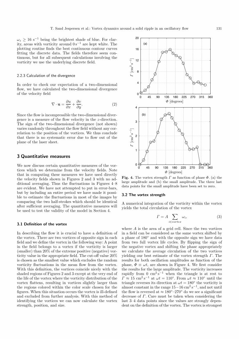
Fig. 4. The vortex strength Γ as function of phase Φ. (a) thelarge amplitude and (b) the small amplitude. The three lastdata points for the small amplitude have been set to zero.

3.2 The vortex strength

A numerical integration of the vorticity within the vortexyields the total circulation of the vortex

Γ = A∑

i∈vortex

ωi, (3)

where A is the area of a grid cell. Since the two vorticesin a field can be considered as the same vortex shifted bya phase of 180◦ and with the opposite sign we have datafrom two full vortex life cycles. By flipping the sign ofthe negative vortex and shifting the phase appropriatelywe calculate the average circulation of the two vorticesyielding our best estimate of the vortex strength Γ . Theresults for both oscillation amplitudes as function of thephase, Φ ≡ ωt, are shown in Figure 4. We first considerthe results for the large amplitude. The vorticity increasesrapidly from 0 cm2 s−1 when the triangle is at rest toΓ ≈ 15 cm2 s−1 at ωt = 110◦. From ωt ≈ 110◦ until thetriangle reverses its direction at ωt = 180◦ the vorticity isalmost constant in the range 15−16 cm2 s−1, and not untilthe flow is reversed at ≈ 180◦–270◦ do we see a significantdecrease of Γ . Care must be taken when considering thelast 3–4 data points since the values are strongly depen-dent on the definition of the vortex. The vortex is strongest


at ωt ≈ 155◦ with a value of Γ Lmax ≈ 16.0 cm2 s−1. When

we compare the data from the two amplitudes we see asimilar qualitative picture although the plateau is less ap-parent at the small amplitude. The maximum Γ for thesmall oscillation amplitude is Γ S

max ≈ 3.5 cm2 s−1.

3.3 The vortex size

By counting the number of grid cells in the vortex we findthe vortex area as shown in Figure 5. The vortices arequite large with widespread vorticity and the vortices aretherefore not intense flow-structures with highly concen-trated vorticity. Consider first the large amplitude. Thearea of the vortex grows concurrently with the buildupof the vortex strength Γ , but the maximum area ofAL

max ≈ 30 cm2 is not reached until ωt ≈ 200◦ whichis later in the period than what we found for the max-imum value of Γ . There is an obvious plateau betweenωt ≈ 150◦ and ωt ≈ 225◦ where the area of the vortex isclose to its maximum value. If we compare the data fromthe two amplitudes we find the same functional form upuntil ωt ≈ 260◦ where the vortex area for the small am-plitude suddenly increases again. This happens becausethe vorticity in the vortex flattens thereby giving an arti-ficially large area, and this effect is relatively larger withthe small amplitude because of smaller values of vortic-ity in the vortices but relatively larger noise in the field.These last data points should be disregarded when con-sidering the area. With the small amplitude we find thatthe maximum area is AS

max ≈ 8 cm2 which is about fourtimes smaller than AL

max.

3.4 The motion of the vortex center

There are several possible definitions of the center of thevortex. The geometric center (the point around which thefluid is rotating) depends on the choice of reference system(the rest system of the triangle or the laboratory system)and it is therefore not a good definition. The vorticity isa differential quantity and does not change when a con-stant velocity is added and is therefore better suited asthe foundation for a definition. The point of maximumvorticity is problematic as vortex center, since there areoften more than one peak within the vortex. Therefore,following [10], we define the center point as a “center ofvorticity” in analogy with the center of mass

rc =A

Γ

∑i∈vortex

ωiri, (4)

where A is the area of a grid cell. The origin of the ref-erence system is taken to be at the tip of the triangle.Figure 6 shows the paths of the two vortices with respectto the triangle. The vortex is moving along the side of thetriangle away from the tip as long as the flow is in the samedirection and at some point the direction is reversed andit moves rapidly along the side of the triangle toward thetip. When it passes the tip, the trajectory bends aroundthe new vortex that is being formed on the new lee sideof the triangle.

0

5

10

15

20

25

30

35

0 45 90 135 180 225 270 315 360

(a)

Φ [degrees]

Vort

exare

a[c

m2]

0

2

4

6

8

10

0 45 90 135 180 225 270 315 360

(b)

Φ [degrees]

Vort

exare

a[c

m2]

Fig. 5. The area of the vortices as defined in Section 3.3.(a) the large amplitude and (b) the small amplitude.

-3

-1.5

0

1.5

3

-12 -8 -4 0 4 8 12

(a)

xc [cm]

yc

[cm

]

-3

-1.5

0

1.5

3

-12 -8 -4 0 4 8 12

(b)

xc [cm]

yc

[cm

]

Fig. 6. The motion of the vortex center relative to the triangle.(a) at the large amplitude and (b) at the small amplitude.

The center motion is resolved in Figure 7 where thecoordinates of the vortex center are shown as a functionof phase. For both amplitudes the direction of each centercoordinate rc = (xc, yc) is reversed at the same instantωt ≈ 155◦ as the strength Γ begins its decline. The non-adiabatic effect, that the vortex reverses direction beforethe triangle does (at ωt = 0◦), shows that the flow aroundthe triangle is strongly history dependent. Comparing the


-15

-10

-5

0

5

10

15

0 45 90 135 180 225 270 315 360

(a)

Φ [degrees]

xc

[cm

]

-2

-1

0

1

2

0 45 90 135 180 225 270 315 360

(b)

Φ [degrees]

yc

[cm

]

-4

-3

-2

-1

0

1

2

3

4

0 45 90 135 180 225 270 315 360

(c)

Φ [degrees]

xc

[cm

]

-2

-1

0

1

2

0 45 90 135 180 225 270 315 360

(d)

Φ [degrees]

yc

[cm

]

Fig. 7. The coordinates xc and yc of the vortex center for the vortices formed on the left and the right side of the triangleas functions of phase. Figures (a) and (b) are for the large amplitude and figures (c) and (d) are for the small amplitude. Thecurves for the vortex formed on the left hand side of the triangle are shifted by a phase of 180◦.

results from the two amplitudes we see that the vortexreaches the same distance in the y-direction but twice thedistance in the x-direction when the amplitude is roughlydoubled.

3.5 Jet velocity

In order to investigate further the increased velocityaround the tip (the jet) due to the presence of the vor-tices we extract the maximal velocity (with respect to thetriangle) vertically below the tip of the triangle. This ve-locity is shown in Figure 8 as a function of phase alongwith the triangle velocity. For both amplitudes the maxi-mum value of the velocity is about 1.6 times the maximumvalue of the driving velocity of the triangle, and the max-imum is reached at a phase about 10◦ before the trianglereaches its maximum velocity.

4 Phenomenological model

4.1 Motivation of the model

The basic variables are the vortex strengths Γ+ and Γ− onthe two sides of the triangle and the velocity U of the fluid

close to the tip (measured relative to the triangle), whichwe shall refer to as the “jet velocity”. Γ+ is always positiveand Γ− is always negative. We only keep track of the vor-ticity until it is advected across the center line. After thatit remains zero until the new vorticity production starts,and we can thus only compare with the measured valuesfrom Section 3.2 up to this point. The external drive hasamplitude d and the horizontal displacement of the trian-gle is x = d cos ωt, so that the unperturbed flow velocityaround the triangle is V0 = dω sin ωt. We assume thatthe relevant time scale is ω−1 and that the flow aroundthe triangle does not depend on the length of the baselineof the triangle and the triangle height, and thus the onlyrelevant length scale is d. We model the vortex strengthsusing the following bilinear differential equation expressedin terms of the dimensionless parameters A1, ... A4:

Γ+ = A1U2θ(V0) − A2ωΓ+

+A3dωUθ(−V0)θ(Γ+) (5)

Γ− = −A1U2θ(−V0) − A2ωΓ−

+A3dωUθ(V0)θ(−Γ−) (6)

U = V0

[1 − A4

ωd2θ(V0)Γ− +

A4

ωd2θ(−V0)Γ+

], (7)


where θ is the familiar Heaviside step function θ(x) = 0for x < 0 and θ(x) = 1 for x > 0. The motivation forthe terms are the following: In equations (5) and (6), theA1-terms express the vorticity production: Γ+ is only pro-duced when U > 0 and Γ− only when U < 0 (since thesquare parenthesis in equation (7) is always positive theseconditions are equivalent to V0 > 0 and V0 < 0, respec-tively). Classical estimates of vortex production [12] giveA1 = 1

2 . It is however well-known that the actual vorticityproduced can be far smaller [13–15]. The classical esti-mate assumes that the velocity close to the solid surfaceis near zero, whereas in reality, the vortex which is createdgenerates a velocity of the same order of magnitude anddirection as the “free stream” there. In addition, it is notclear which fraction of the available vorticity will actuallybe entrained behind the solid triangle and become caughtup in the separation vortex. In the following we shall thusregard A1 as a phenomenological parameter.

The A2-terms describe exponential damping due toviscosity or turbulent fluctuations. It is always present.The A3-terms express the decay of vorticity due to ad-vection. For the vortex formed on the right with Γ+ ≥ 0the A3-term in equation (5) is active when the velocity Uaround the triangle is negative. The coefficient A3 is itselfpositive and since the A3-term is proportional to U it isnegative during the half-period when Γ+ decays. Similarlyfor the A3-term in equation (6) which is positive duringthe half-period when the negative vortex formed on theleft side of the triangle decays. Thus the A3-term alwaysacts to reduce the absolute value of the vorticity. The A4-terms in equation (7) are included since we assume thatvorticity upwind of the tip enhances the jet. We simplytake it to be proportional to the driving velocity and thevorticity present. In reality this term describes a compli-cated interaction, which depends on the detailed shapeand motion of the vortices.

4.2 Scaling

We now use dimensionless time τ = ωt, and correspond-ingly we introduce dimensionless vortex strengths y± suchthat Γ± = ωd2by± and a dimensionless velocity u suchthat U = ωdau, where a and b are additional dimension-less scaling parameters to be fixed below. In terms of thesenew variables we obtain

y+ =A1a

2

bu2θ(V0) − A2y+ +

A3a

buθ(−V0)θ(y+) (8)

y− = −A1a2

bu2θ(−V0) − A2y− +

A3a

buθ(V0)θ(−y−)

(9)

u =V0

ωda[1 − A4bθ(V0)y− + A4bθ(−V0)y+] , (10)

where the dot now means derivative with respect to τ ,which we denote by t in the following, since we shall onlyuse the scaled variables. It is natural to take a = 1 becausethen the driving term has the simple form: V0/ωad = sin t.

-30

-20

-10

0

10

20

30

0 45 90 135 180 225 270 315 360

(a)

Φ [degrees]

vel

oci

ty[c

ms−

1]

-15

-10

-5

0

5

10

15

0 45 90 135 180 225 270 315 360

(b)

Φ [degrees]

vel

oci

ty[c

ms−

1]

Fig. 8. The solid line shows the velocity of the triangle andthe solid line with circles shows the jet velocity, i.e., the max-imal x-velocity vertically below the triangle tip. (a) the largeamplitude and (b) the small amplitude.

Further, we choose the coefficient A1a2

b for the vortex pro-duction term to be unity and thus b = A1. The final formis then

y+ = u2θ(sin t) − b2y+ + b3uθ(− sin t)θ(y+) (11)

y− = −u2θ(− sin t) − b2y− + b3uθ(sin t)θ(−y−) (12)

u = sin t [1 − b4θ(sin t)y− + b4θ(− sin t)y+] , (13)

where we have

b2 = A2, b3 =A3

A1, b4 = A4A1 . (14)

4.3 Numerical solution

Typical numerical solutions are shown in Figure 9. Inter-esting periodic solutions exist only within a small param-eter region. If the vorticity production is small U and V0

become almost identical. If, on the other hand, the vortic-ity production becomes too large, the vorticity cannot beswept away by the jet and it can increase without bound.It seems that the interesting states – those that look likethe experiments – are very close to the “critical point”


-1,5

-1

-0,5

0

0,5

1

1,5

0 1 2 3 4 5 6

y+

y-

V0

U

velo

city

/circ

ulat

ion

Φ

(a)

-1,5

-1

-0,5

0

0,5

1

1,5

0,1 0,3 0,5 0,7 0,9

y+

y-

V0

U

velo

city

/circ

ulat

ion

Φ

(b)

Fig. 9. Solution of equations (11–13). Figure (a) initial cy-cles starting from rest and figure (b) final periodic state.The parameters are b2 = 0.3/2π ≈ 0.0484, b3 = 1.0 andb4 = 2.15/2π ≈ 0.34. The circulations y± have been scaledby 2.968 to give a maximal value of 1.

where the vorticity diverges. In other words, the experi-mentally relevant states seem to correspond to particularcombinations of the parameters b2...b4. In this sense, it be-haves like a self-resonating system [16]. In Section 4.4 weshall find the allowed combinations of parameters in theundamped case, where the model can be solved exactly.

4.4 Analytic solution for b2 = 0

We now discuss analytically the special case b2 = 0, i.e.,no damping due to viscosity (there is still damping due to

advection represented by b3). We get

y+ = u2θ(sin t) + b3uθ(− sin t)θ(y+) (15)

y− = −u2θ(− sin t) + b3uθ(sin t)θ(−y−) (16)

u = sin t [1 − b4θ(sin t)y− + b4θ(− sin t)y+] . (17)

4.4.1 General analytic solution

To find the solution for an arbitrary period[2nπ, 2(n + 1)π], it has to be split into four parts [2nπ, t∗],[t∗, (2n + 1)π],

[(2n + 1)π, t∗

]and

[t∗, 2(n + 1)π

].

The solution for t ∈ [2nπ, (2n + 1)π] is, first for y−:

y−(t) =

{1α (1 − u∗e−β(1−cos t)) for 2nπ < t < t∗

0 for t∗ < t < (2n + 1)π,(18)

where for convenience α = b4 and β = b3b4. The constantu∗ = 1 − αy∗, where we define y∗ = y−(2nπ). If y−(t)becomes zero somewhere in the interval, at t = t∗, it willremain so. The solution for y− in the remaining interval is

y−(t) =

−(u∗)2∫ t

(2n+1)πe−2β(1+cos t′) sin2 t′ dt′

for (2n + 1)π < t < t∗

y−(t∗) − 12 (t − t∗) + 1

4 (sin 2t − sin 2t∗)

for t∗ < t < 2(n + 1)π

(19)

where t∗ will be defined later.For u we get

u(t) =

u∗e−β(1−cos t) sin t for 2nπ < t < t∗sin t for t∗ < t < (2n + 1)πu∗e−β(1+cos t) sin t for (2n + 1)π < t < t∗

sin t for t∗ < t < 2(n + 1)π.(20)

Finally, we get for y+:

y+(t) = (u∗)2∫ t

2nπ

e−2β(1−cos t′) sin2 t′ dt′ , (21)

which is valid for t < t∗. For t ∈ [t∗, (2n + 1)π] we have

y+(t) = y+(t∗) +∫ t

t∗sin2 t′dt′

= y+(t∗) +12(t − t∗) − 1

4(sin 2t − sin 2t∗). (22)

Similarly we get for t ∈ [(2n + 1)π, 2(n + 1)π]

y+(t) =

{− 1α (1 − u∗e−β(1+cos t)) for (2n + 1)π < t < t∗

0 for t∗ < t < 2(n + 1)π(23)

where u∗ = 1 + αy∗ and y∗ = y+(2nπ + π).


4.4.2 Integral equation for t∗ in the periodic state

In the periodic state we have y∗ = −y∗, u∗ = u∗ andt∗ = t∗ + π. Note the symmetry of the periodic state:

u(t + π) = −u(t) (24)y−(t + π) = −y+(t). (25)

As can be seen u is not differentiable at t = nπ in the pe-riodic state. In fact u′(π−) = −1 and u′(π+) = −u∗. Theexistence of a t∗ where all the vorticity has been “blown”away is necessary for attaining a periodic state, since oth-erwise vorticity will accumulate and lead to divergent so-lutions. For a t∗ to exist we must have

1 − cos t∗ =1β

ln(u∗). (26)

The existence of a periodic state is governed by thefollowing integral equation for y∗ (or u∗) and t∗ obtainedusing equation (25)

u∗ − 1α

=

(u∗)2e−2β

∫ t∗

0

e2β cos t sin2 t dt +12(π − t∗) +

14

sin 2t∗.

(27)

This equation together with the relation (26) can be com-bined to give one final equation for t∗:

eβ(1−cos t∗) − 1 =

α

[∫ t∗

0

e2β(cos t−cos t∗) sin2 t dt +12(π − t∗) +

14

sin 2t∗]

.

(28)

To have physical solutions we must have π/2 < t∗ < π.The upper limit t∗ = π gives

α+ =1 − e−2β∫ π

0 e2β cos t sin2 t dt

=2β

π

(1 − e−2β)I1(2β)

=2π

1 − e−2β

I0(2β) − I2(2β), (29)

where I0, I1, and I2 are Bessel functions. The interestingsolutions, in the sense that they are resonant, i.e., givelarge amplitudes, have t∗ close to π (at least within theinterval 3π/4 < t∗ < π). Figure 10 shows the two linesα = α(β) corresponding to, t∗ = π (solid line) and t∗ =3π/4 (dashed line), respectively. The meaningful solutionsoccur between these two curves for β < β∗ ≈ 0.385, wherethey cross.

Figure 11 shows a typical numerical solution for theperiodic state at β = 0.25 and α = 0.2387 (and no damp-ing), which as can be seen in Figure 12 lies in the allowedregion of the phase diagram. It is well represented by theanalytical solution in Section 4.4.

0

0,1

0,2

0,3

0,4

0 0,1 0,2 0,3 0,4 0,5

t* = 3π/4

t* = π

α

β

Fig. 10. Phase diagram in the variables β = b3b4 and α = b4.The solid line shows t∗ = π and the dashed line t∗ = 3π/4.The meaningful solutions occur between these curves beforethe lines cross at β = β∗.

-1,5

-1

-0,5

0

0,5

1

1,5

0,1 0,3 0,5 0,7 0,9

y+

y-

V0

U

velo

city

/circ

ulat

ion

Φ

Fig. 11. Solution of equations (11–13) with b2 = 0. Finalperiodic state with β = 0.25 and α = 0.2387.

4.5 Maximal value of u

Experimentally, the maximal value of u is umax ≈ 1.6.The maximal value can be found from equation (20). Thefunction sin(t) exp(β cos t) has a maximum when cos t −β(sin2 t) = β cos2 t + cos t − β = 0 or

cos t =12β

(−1 ±

√1 + 4β2

), (30)

which means that the phase φ where u is maximal is

φ = arccos[

12β

(−1 ±

√1 + 4β2

)], (31)


-0,2

0

0,2

0,4

0,6

0,8

1

1,2

30 80 130 180 230 280 330

Γ+

Γsmall

Γlarge

Γ

Φ [degrees]

Fig. 12. The theoretical and the experimental circulation asfunction of time. The experimental data sets have been scaledas described in the text.

with one solution (choosing the plus sign) φ ∈ [0, π/2].Then

umax = u∗e−β(1−cosφ) sin φ

=u∗ 1√2β

√(√

1+4β2−1)e(√

1+4β2−2β−1)/2. (32)

4.6 Comparison with experiment

In the experiment we have ω = π s−1 and the two am-plitudes dS = 2.5 cm and dL = 4.6 cm. The maximalmeasured vortex strengths are Γ S

max = 3.5 cm2 s−1 andΓ L

max = 16.0 cm2 s−1. In the comparison we use the scalingfrom Section 4.2, i.e., Γ± = A1ωd2y±. In the state corre-sponding to the numerical solution in Figure 9, we havemaximal values of y± around 3 and we find that A1 ≈ 0.07(see also the discussion of A1 in Sect. 4.1). In Figure 12we show a comparison between the circulations from theexperiment and the numerical solution corresponding toFigure 9. We have scaled the theoretical circulation as inFigure 9 (to make the maximum unity) and we have scaledthe experimental circulations by factors 13.73 cm2 s−1 and4.06 cm2 s−1 with the ratio (dL/dS)2 according to the scal-ing assumptions of Section 4.2. It is seen that the generalform and the position of the maximum are well repro-duced.

In Figure 13 we compare the velocities. Here the ex-perimental velocities (Fig. 8) are scaled by ωd, i.e., by14.45 cm s−1 and 7.86 cm s−1, respectively. Again the simi-larity between experiment and theory is surprisingly good,considering the very simple character of the latter.

-2

-1,5

-1

-0,5

0

0,5

1

1,5

2

30 80 130 180 230 280 330

V0

UV

large

Vsmall

jet v

eloc

ity

Φ [degrees]

Fig. 13. The theoretical end the experimental curves for thejet-velocity. The parameters of the model are as in Figure 9.The experimental data sets have been scaled as described inthe text.

5 Discussion and conclusions

The generation of vortices, or separation zones, around pe-riodically moving solid structures, is a surprisingly violentprocess. In particular, the initiation of a vortex dependsstrongly on the localized jet which is formed slightly af-ter the triangle has reversed its direction of motion. Wehave developed a simple phenomenological model for thegeneration of the vortices and their interaction with thejet, which can be solved exactly in the limit of no viscousdamping and which compares favorably with our exper-imental results. Our results emphasize the non-adiabaticand history dependent character of the formation of sep-aration zones in time-dependent flows, which means thatthis process can not be captured by steady state calcula-tions.

The phenomenology described and modeled in this pa-per is important for the development of quantitative mod-els of the formation and evolution of “vortex ripples” inthe sand under oscillating water flow. In particular it isimportant for understanding the instabilities, which oc-cur when the oscillatory drive changes [5], leading, e.g., tothe creation of new ripples in the troughs between the oldones that already exist. Here the strength and size of theseparation vortex determines the position and growth ofthe new ripple. In this context, it would be of great inter-est to extend our model to two dimensions, and includethe instabilities which occur in the transverse directionand deform the cylindrical separation vortex.

Another problem for which our results might be rele-vant is insect flight, i.e., the generation of lift and thrustby flapping wings at intermediate Reynolds numbers [6–8].Here the nature and strength of the separation vortices


(so-called leading edge vortices) is of primary importance,and non-adiabatic effects are known to be large.

We are very thankful to Knud Erik Meyer and Nicolas Pedersenfor making the PIV equipment at the Department of FluidMechanics at the Technical University of Denmark available tous and for their crucial help in carrying out the experiment. A.A. acknowledges the support from AFOSR Grant No. F49620-01-1-0530 and ONR Grant No. N00014-01-1-0688 granted toZ. Jane Wang.

References

1. D.I. Pullin, A.E. Perry, J. Fluid Mech. 97, 239 (1980)2. H. Ayrton, Proc. Roy. Soc. A 84, 285 (1910)3. R.A. Bagnold, Proc. Roy. Soc. A 187, 1 (1946)4. A. Stegner, J.E. Wesfreid, Phys. Rev. E 60, R3487 (1999)5. J.L. Hansen, M. van Hecke, A. Haaning, C. Ellegaard,

K.H. Andersen, T. Bohr, T. Sams, Nature 410, 324(2001); J.L. Hansen, M. van Hecke, C. Ellegaard, K.H.Andersen, T. Bohr, A. Haaning, T. Sams, Phys. Rev.Lett. 87, 204301 (2001)

6. C.P. Ellington, C. van den Berg, A.P. Willmott, A.L.R.Thomas, Nature 384, 626 (1996)

7. M.H. Dickinson, F.-O. Lehmann, S.P. Sane, Science 284,1954 (1999)

8. Z.J. Wang, Phys. Rev. Lett. 85, 2216 (2000)9. H.C. Earnshaw, T. Bruce, C.A. Greated, W.J. Easson,

Proc. of the 24th Int. Conf. of Coastal Engineering,p. 1975 (1994)

10. H.C. Earnshaw, C.A. Greated, Exp. Fluids 25, 265 (1998)11. M. Raffel, C.E. Willert, J. Kompenhans, Particle Image

Velocimetry (Springer-Verlag, Berlin, Heidelberg, 1998)12. L. Prandtl, O.G. Tietjens, Fundamentals of Hydro- and

Aeromechanics (Dover, New York, 1957)13. N. Didden, J. Applied Math. Phys. (ZAMP) 30, 101

(1979)14. M. Gharib, E. Rambod, K. Shariff, J. Fluid Mech. 360,

121 (1998)15. M. Rosenfeld, E. Rambod, M. Gharib, J. Fluid Mech.

376, 297 (1998)16. A. Boudaoud, Y. Couder, M. Ben Amar, Phys. Rev. Lett.

82, 3847 (1999)

Documents

Vortex dynamics around a solid ripple in an oscillatory flow