Embed Size (px)
Citation preview
1
Algorithmic Networks & Optimization
Maastricht, November 2008
Ronald L. Westra, Department of MathematicsMaastricht University
2
Network Models
3
Properties of Networks
4
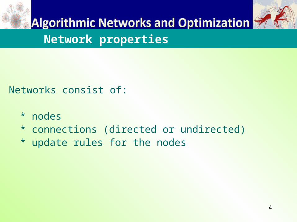
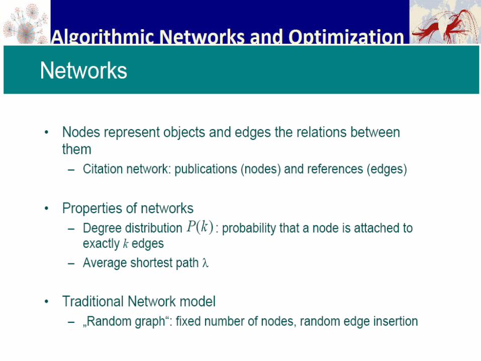
Networks consist of:
* nodes * connections (directed or undirected)* update rules for the nodes
Network properties
5
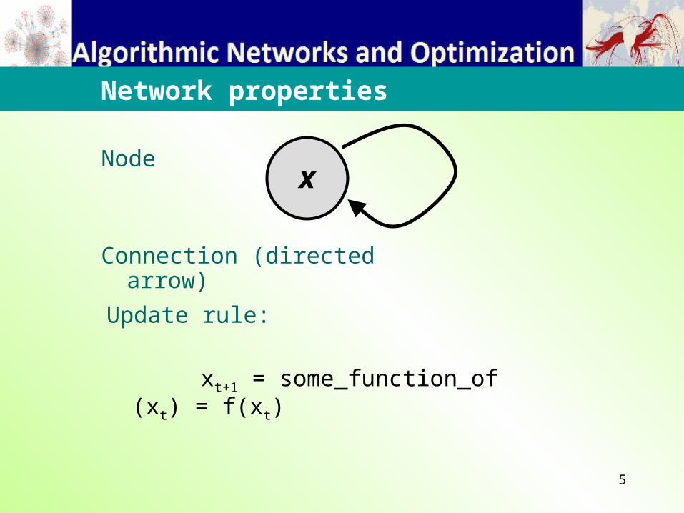
Node
Network properties
x
Connection (directed arrow)
Update rule:
xt+1 = some_function_of (xt) = f(xt)

6
Until now we have encountered a number of interesting models
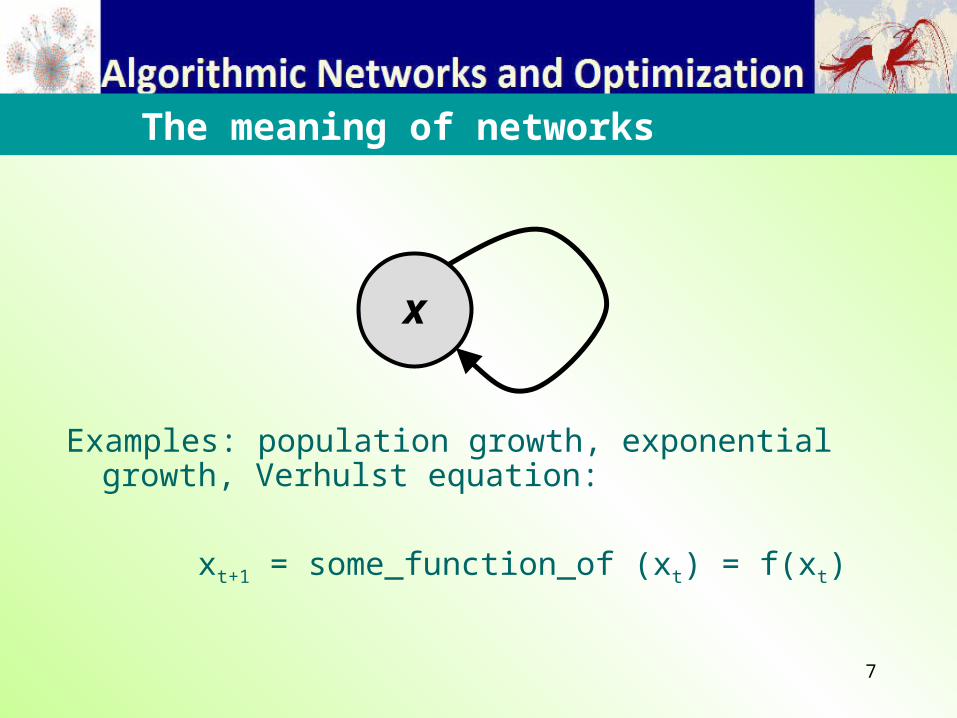
1 entity that interacts only with itself
The meaning of networks
x
7
Examples: population growth, exponential growth, Verhulst equation:
xt+1 = some_function_of (xt) = f(xt)
The meaning of networks
x
8
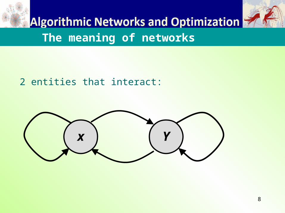
2 entities that interact:
The meaning of networks
Yx
9
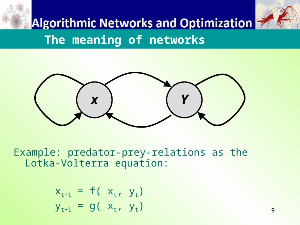
Example: predator-prey-relations as the Lotka-Volterra equation:
xt+1 = f( xt, yt)
yt+1 = g( xt, yt)
The meaning of networks
Yx
10
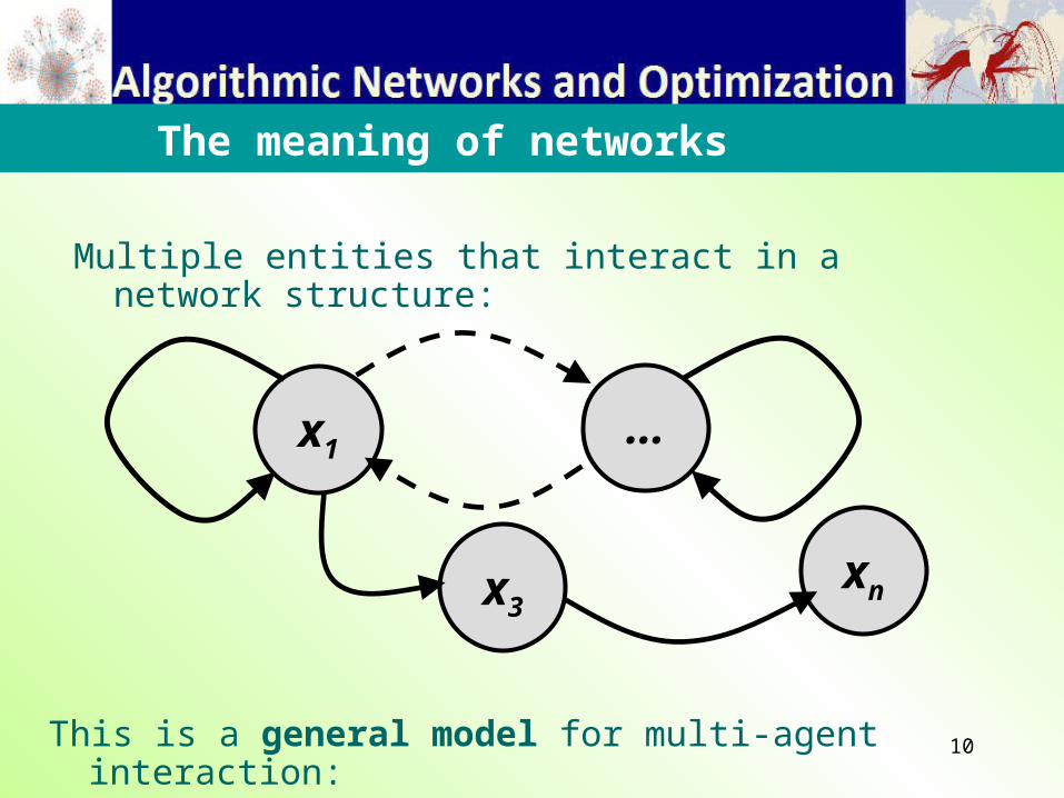
Multiple entities that interact in a network structure:
The meaning of networks
This is a general model for multi-agent interaction:
…x1
x3xn
11
Small-World Networks
12
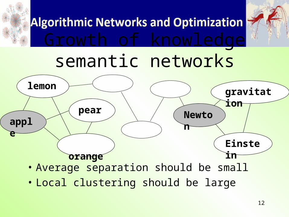
Growth of knowledgesemantic networks
apple
orange
pear
lemon
Newton
Einstein
gravitation
• Average separation should be small
• Local clustering should be large
13
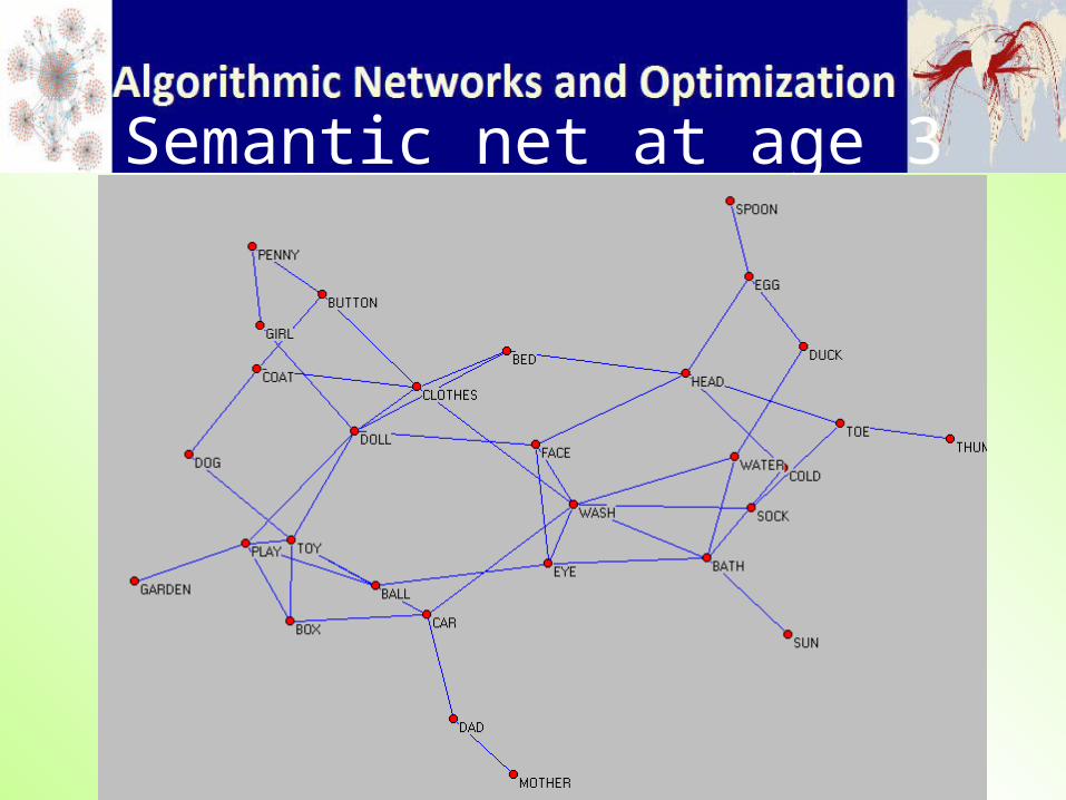
Semantic net at age 3
14
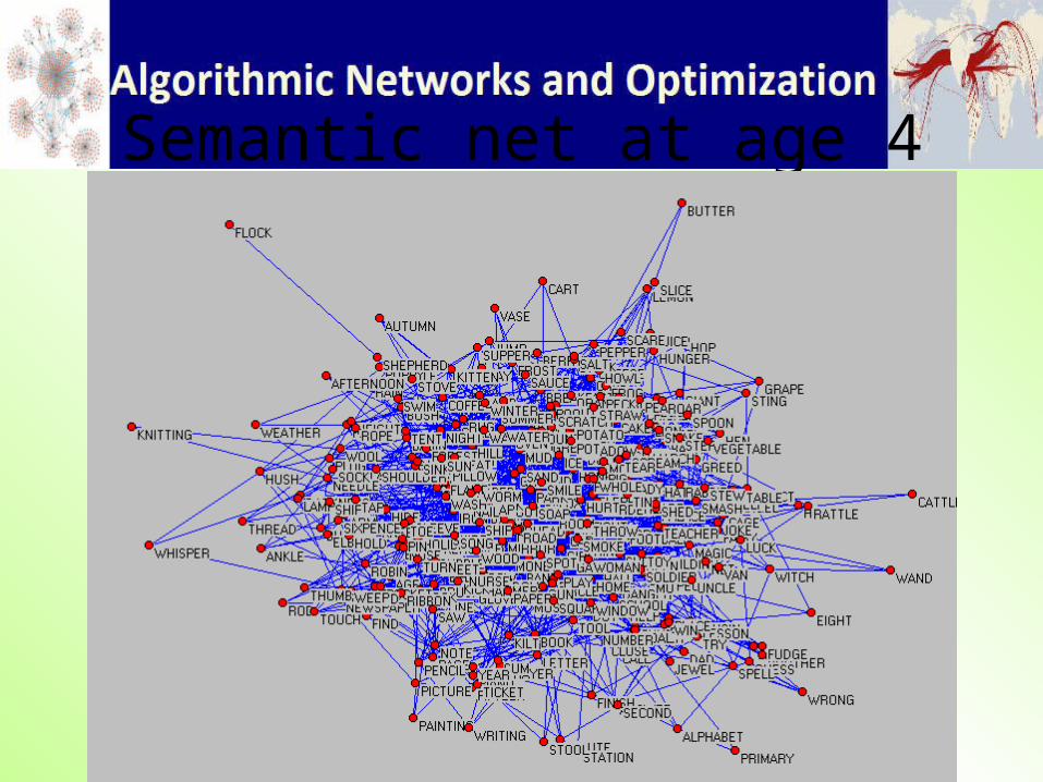
Semantic net at age 4
15
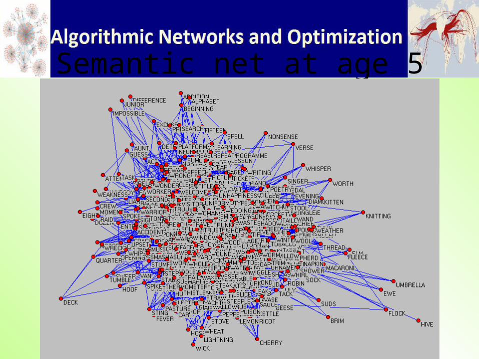
Semantic net at age 5
16
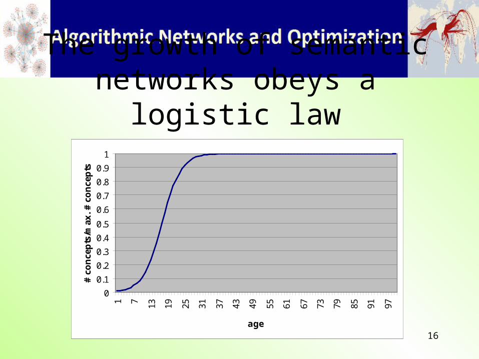
The growth of semantic networks obeys a logistic law
0
0.1
0.2
0.3
0.4
0.5
0.6
0.7
0.8
0.9
1
1 7 13 19 25 31 37 43 49 55 61 67 73 79 85 91 97
age
# co
nce
pts
/max
. #
con
cep
ts
17
Given the enormous size of our semantic networks, how do we associate two arbitrary concepts?
18
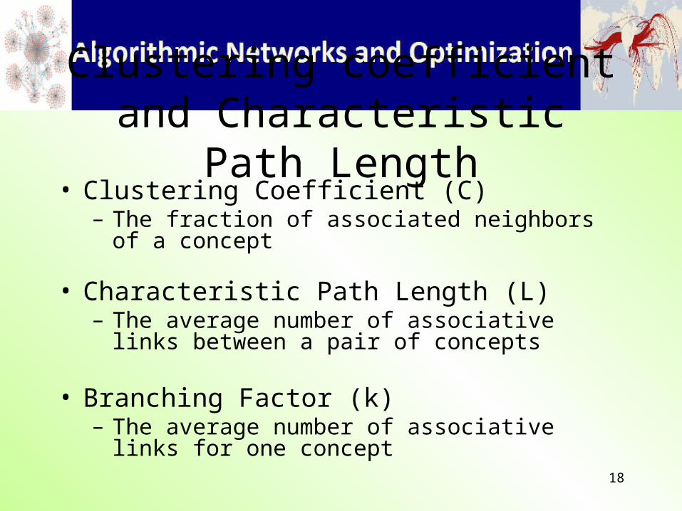
Clustering coefficient and Characteristic Path Length
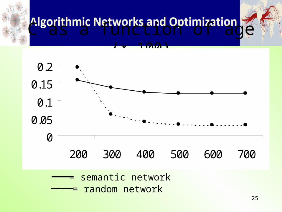
• Clustering Coefficient (C) – The fraction of associated neighbors of a concept
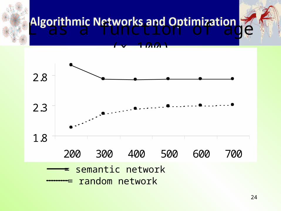
• Characteristic Path Length (L)– The average number of associative links between a pair
of concepts
• Branching Factor (k)– The average number of associative links for one
concept
19
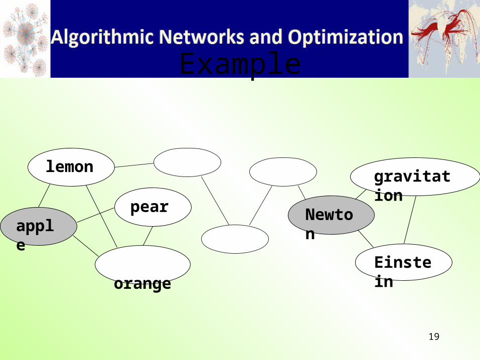
Example
apple
orange
pear
lemon
Newton
Einstein
gravitation
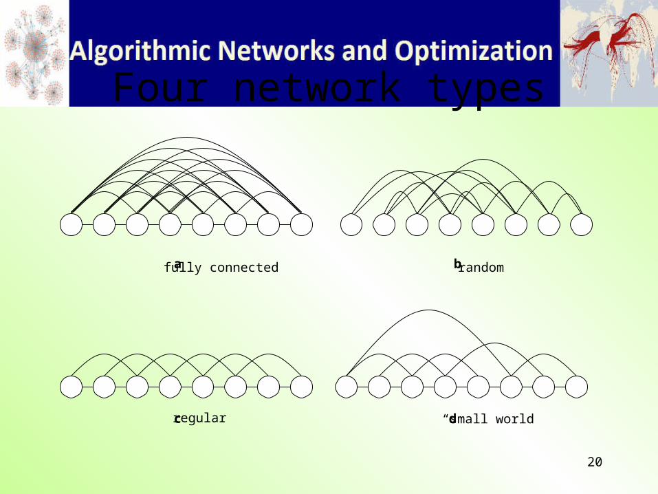
20
Four network types
a
c
b
d
fully connected random
regular “small world
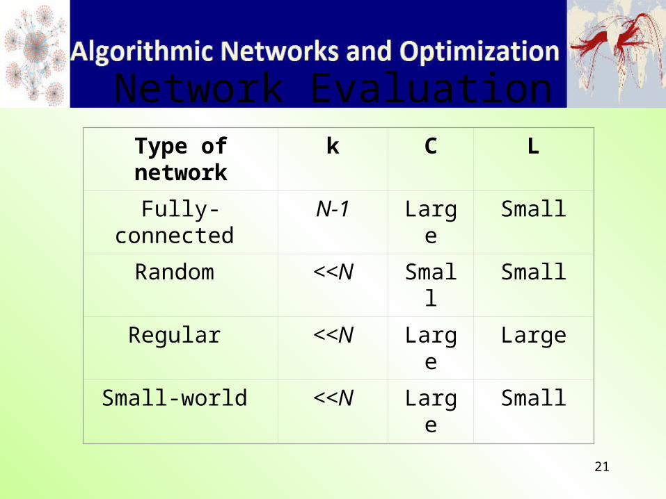
21
Network EvaluationType of network k C L
Fully-connected N-1 Large Small
Random <<N Small Small
Regular <<N Large Large
Small-world <<N Large Small
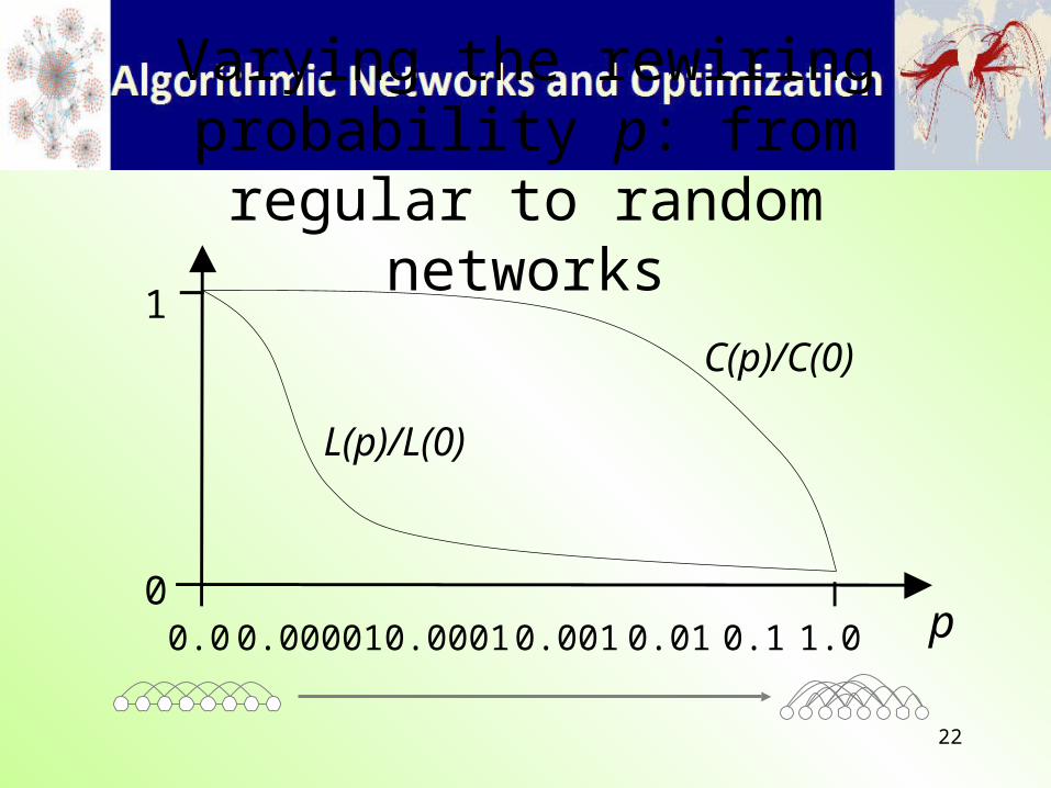
22
Varying the rewiring probability p: from regular to random networks
C(p)/C(0)
L(p)/L(0)
1
0 p
0.00001 0.10.010.0010.0001 1.00.0
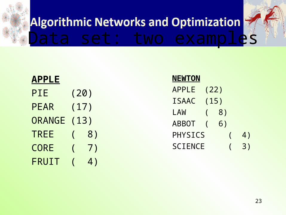
23
Data set: two examples
APPLE
PIE (20)
PEAR (17)
ORANGE (13)
TREE ( 8)
CORE ( 7)
FRUIT ( 4)
NEWTON
APPLE (22)
ISAAC (15)
LAW ( 8)
ABBOT ( 6)
PHYSICS( 4)
SCIENCE ( 3)
24
L as a function of age (× 100)
1.8
2.3
2.8
200 300 400 500 600 700
= semantic network= random network
25
C as a function of age (× 100)
0
0.05
0.1
0.15
0.2
200 300 400 500 600 700
= semantic network= random network
26
Small-worldlinessWalsh (1999)
• Measure of how well small path length is combined with large clustering
• Small-wordliness = (C/L)/(Crand/Lrand)
27
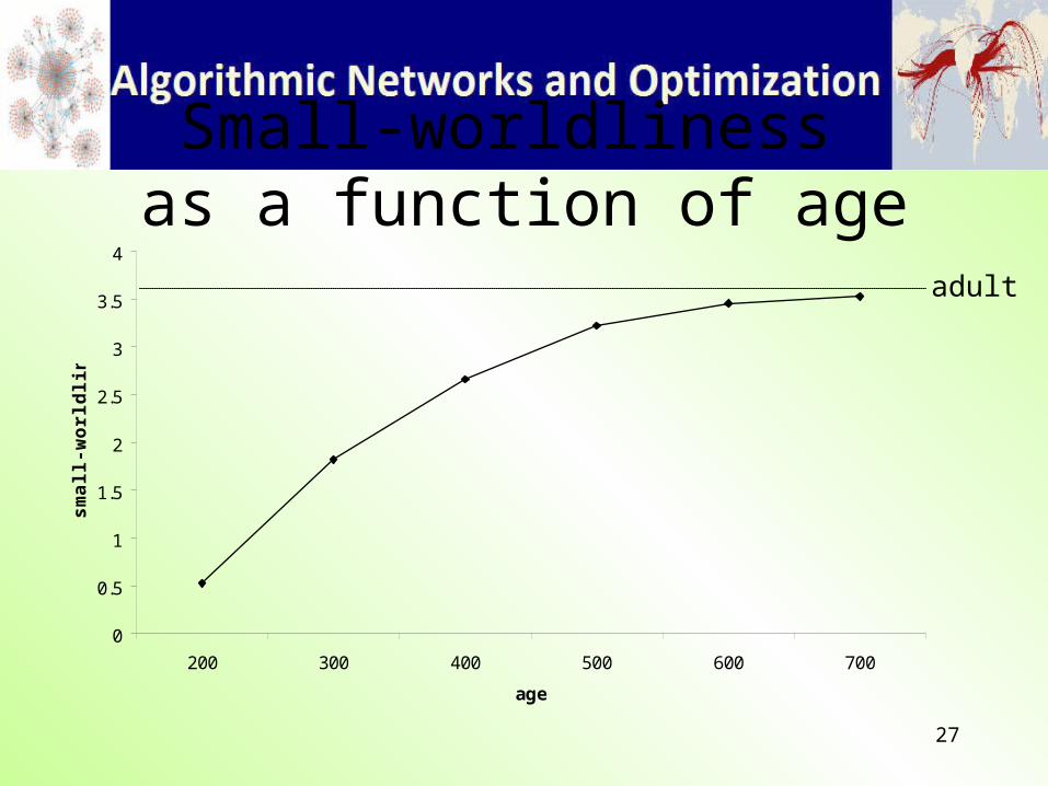
Small-worldliness as a function of age
0
0.5
1
1.5
2
2.5
3
3.5
4
200 300 400 500 600 700
age
sm
all
-wo
rld
lin
es
s
adult
28
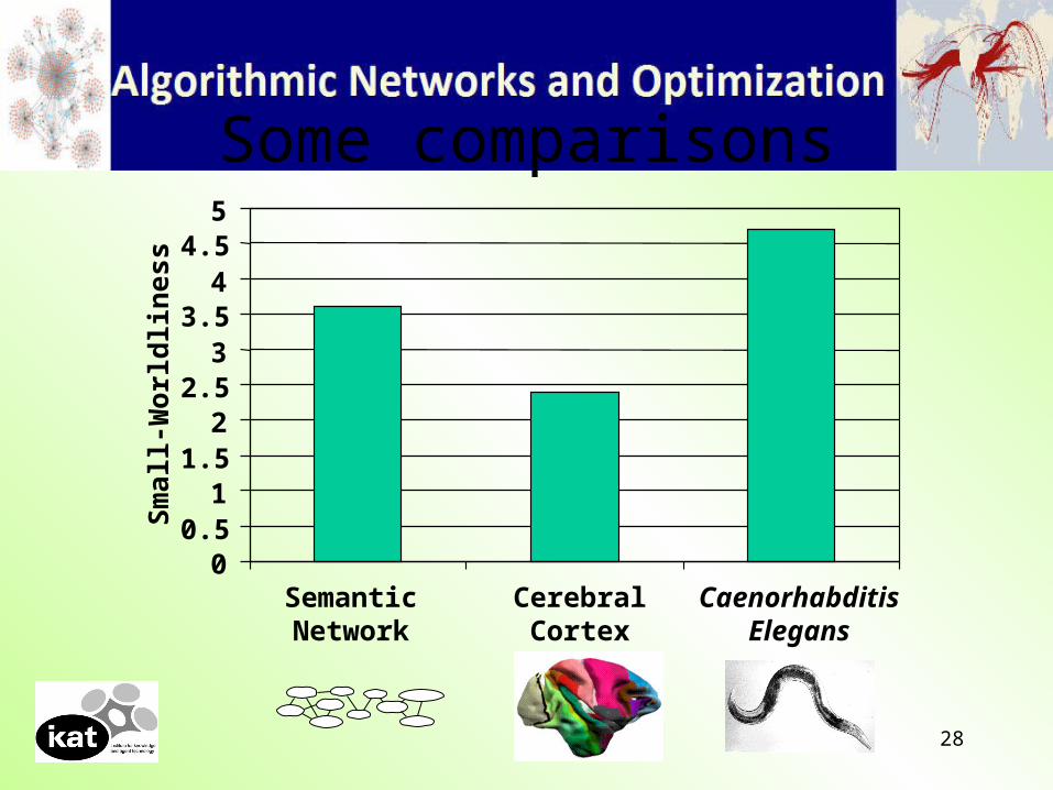
Some comparisons
00.5
11.5
22.5
33.5
44.5
5
SemanticNetwork
CerebralCortex
CaenorhabditisElegans
Sm
all-
Wor
ldli
nes
s
29
What causes the small-worldliness in the semantic net?
• TOP 40 of concepts
• Ranked according to their k-value (number of associations with other concepts)
30
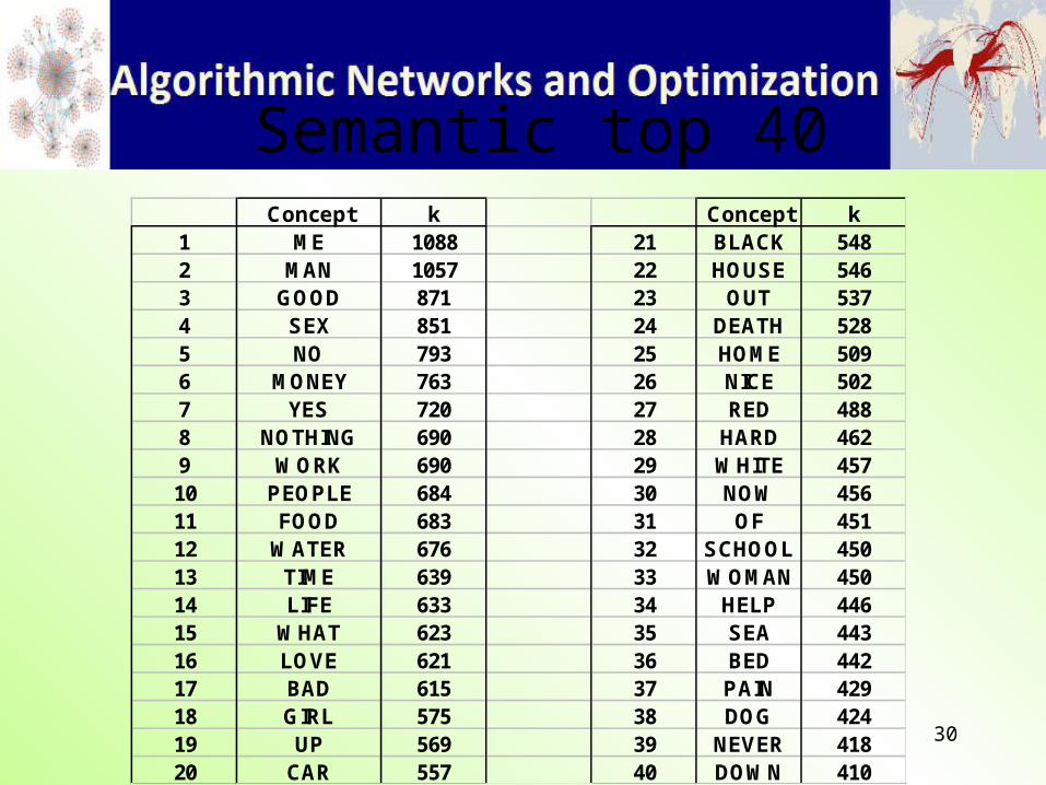
Semantic top 40Concept k Concept k
1 ME 1088 21 BLACK 5482 MAN 1057 22 HOUSE 5463 GOOD 871 23 OUT 5374 SEX 851 24 DEATH 5285 NO 793 25 HOME 5096 MONEY 763 26 NICE 5027 YES 720 27 RED 4888 NOTHING 690 28 HARD 4629 WORK 690 29 WHITE 45710 PEOPLE 684 30 NOW 45611 FOOD 683 31 OF 45112 WATER 676 32 SCHOOL 45013 TIME 639 33 WOMAN 45014 LIFE 633 34 HELP 44615 WHAT 623 35 SEA 44316 LOVE 621 36 BED 44217 BAD 615 37 PAIN 42918 GIRL 575 38 DOG 42419 UP 569 39 NEVER 41820 CAR 557 40 DOWN 410
31
32
Special Networks
33
Special Networks
• Small-world networks
• Scale-free networks
34
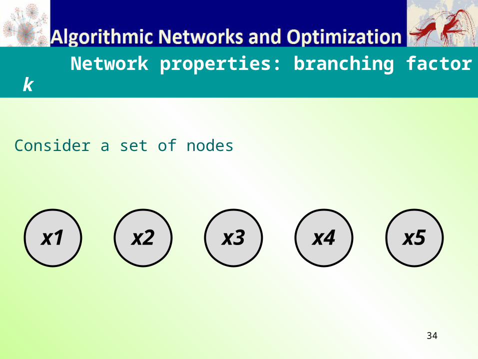
Consider a set of nodes
Network properties: branching factor k
x1 x2 x3 x4 x5
35
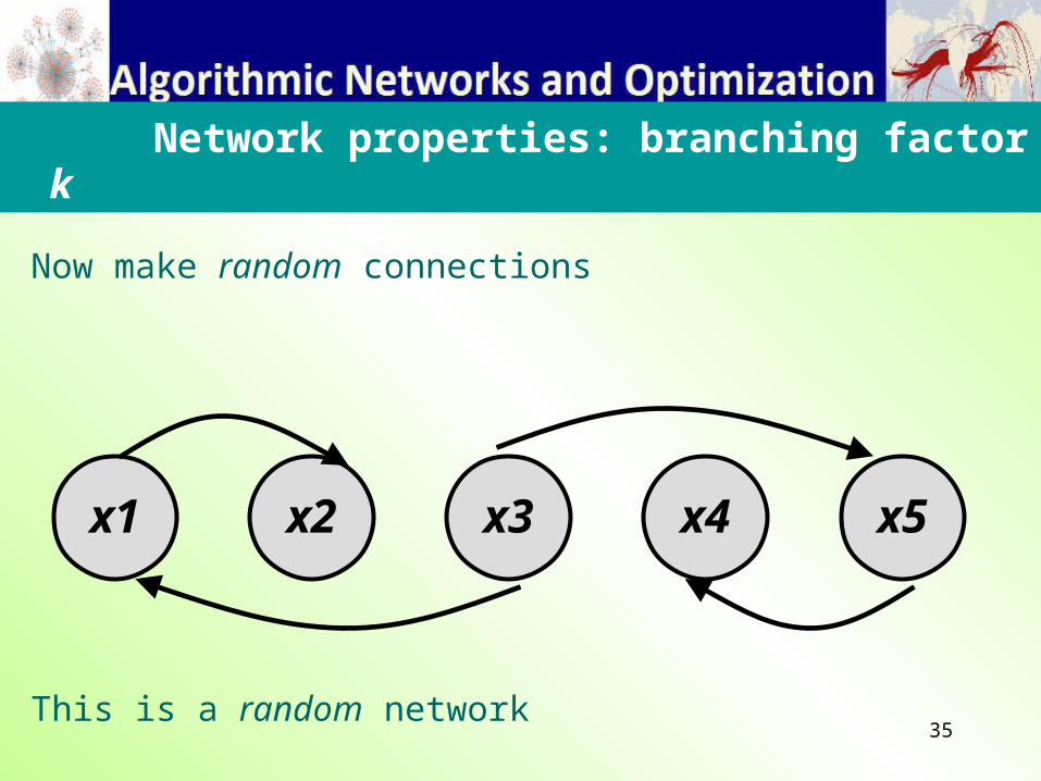
Now make random connections
Network properties: branching factor k
x1 x2 x3 x4 x5
This is a random network
36
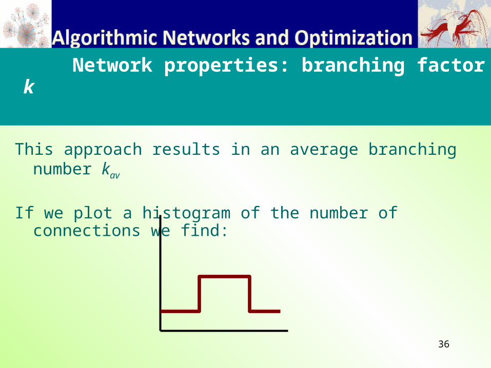
This approach results in an average branching number kav
If we plot a histogram of the number of connections we find:
Network properties: branching factor k
37
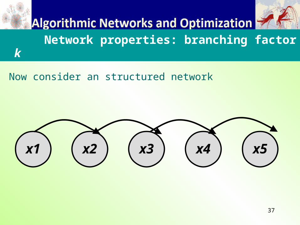
Now consider an structured network
Network properties: branching factor k
x1 x2 x3 x4 x5
38
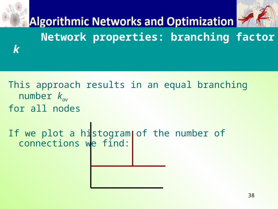
This approach results in an equal branching number kav
for all nodes
If we plot a histogram of the number of connections we find:
Network properties: branching factor k
39
The same for a fully connected network:
this results in an equal branching number kav = n - 1
Network properties: branching factor k
40
Now what for a small-world network?
Network properties: branching factor k
41
HistoryUsing a Web crawler, physicist Albert-László Barabási at the
University of Notre Dame mapped the connectedness of the Web in 1999 (Barabási and Albert, 1999).
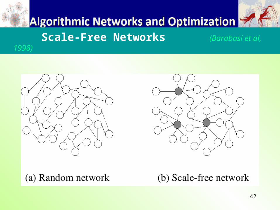
To their surprise, the Web did not have an even distribution of connectivity (so-called "random connectivity"). Instead, some network nodes had many more connections than the average; seeking a simple categorical label, Barabási and his collaborators called such highly connected nodes "hubs".
Scale-Free Networks (Barabasi et al, 1998)
42
Scale-Free Networks (Barabasi et al, 1998)
43
History (Ctd)
In physics, such right-skewed or heavy-tailed distributions often have the form of a power law, i.e., the probability P(k) that a node in the network connects with k other nodes was roughly proportional to k−γ, and this function gave a roughly good fit to their observed data.
Scale-Free Networks (Barabasi et al, 1998)
44
History (Ctd)
After finding that a few other networks, including some social and biological networks, also had heavy-tailed degree distributions, Barabási and collaborators coined the term "scale-free network" to describe the class of networks that exhibit a power-law degree distribution.
Soon after, Amaral et al. showed that most of the real-world networks can be classified into two large categories according to the decay of P(k) for large k.
Scale-Free Networks (Barabasi et al, 1998)
45
A scale-free network is a noteworthy kind of complex network because many "real-world networks" fall into this category.
“Real-world" refers to any of various observable phenomena that exhibit network theoretic characteristics (see e.g., social network, computer network, neural network, epidemiology).
Scale-Free Networks (Barabasi et al, 1998)

46
In scale-free networks, some nodes act as "highly connected hubs" (high degree), although most nodes are of low degree.
Scale-free networks' structure and dynamics are independent of the system's size N, the number of nodes the system has. In other words, a network that is scale-free will have the same properties no matter what the number of its nodes is.
Scale-Free Networks (Barabasi et al, 1998)
47
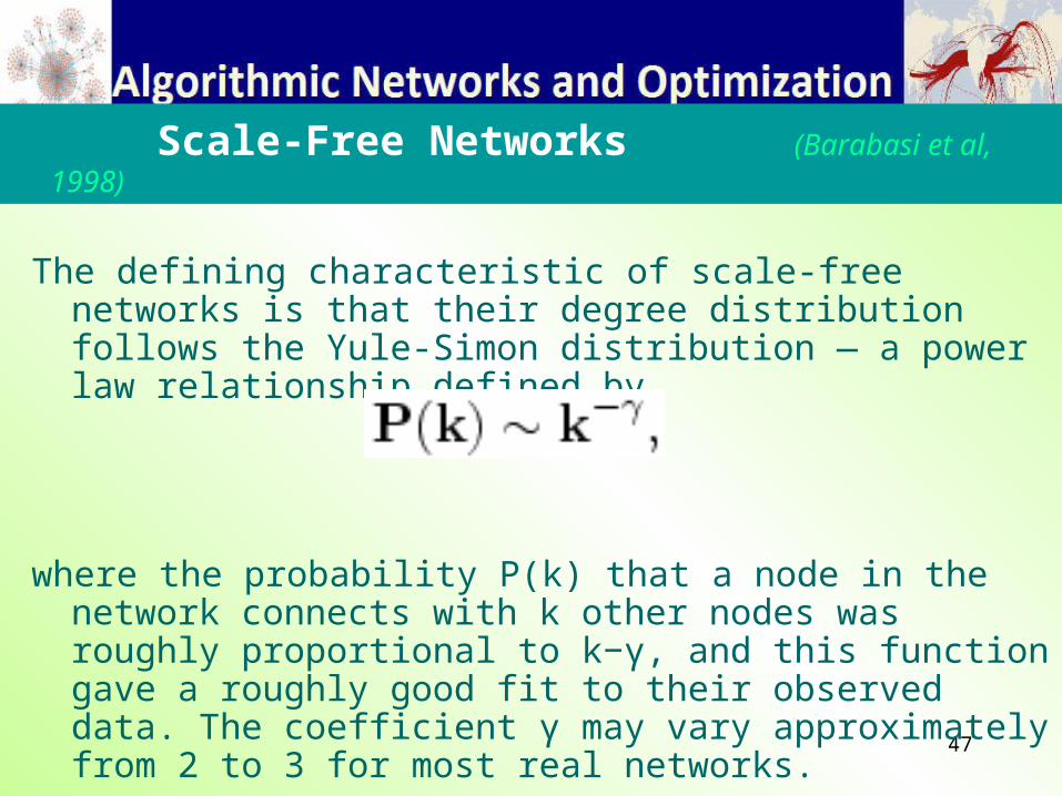
The defining characteristic of scale-free networks is that their degree distribution follows the Yule-Simon distribution — a power law relationship defined by
where the probability P(k) that a node in the network connects with k other nodes was roughly proportional to k−γ, and this function gave a roughly good fit to their observed data. The coefficient γ may vary approximately from 2 to 3 for most real networks.
Scale-Free Networks (Barabasi et al, 1998)
48
49
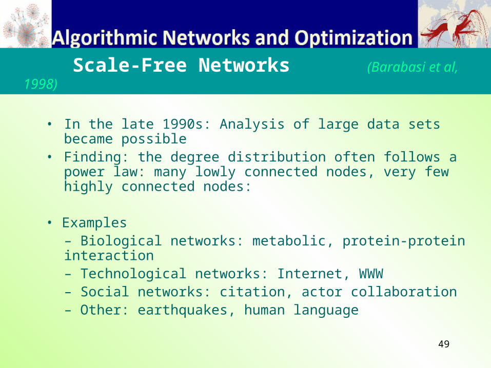
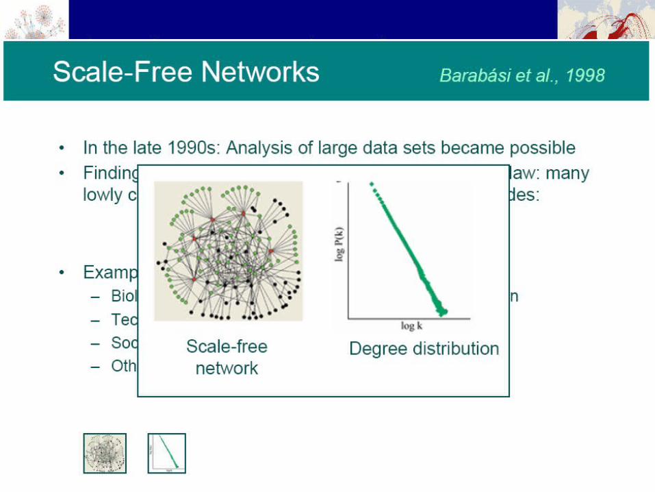
• In the late 1990s: Analysis of large data sets became possible• Finding: the degree distribution often follows a power law: many
lowly connected nodes, very few highly connected nodes:
• Examples– Biological networks: metabolic, protein-protein interaction– Technological networks: Internet, WWW– Social networks: citation, actor collaboration– Other: earthquakes, human language
Scale-Free Networks (Barabasi et al, 1998)
50
51
52
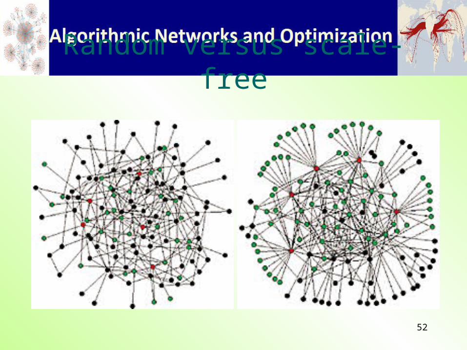
Random versus scale-free
53
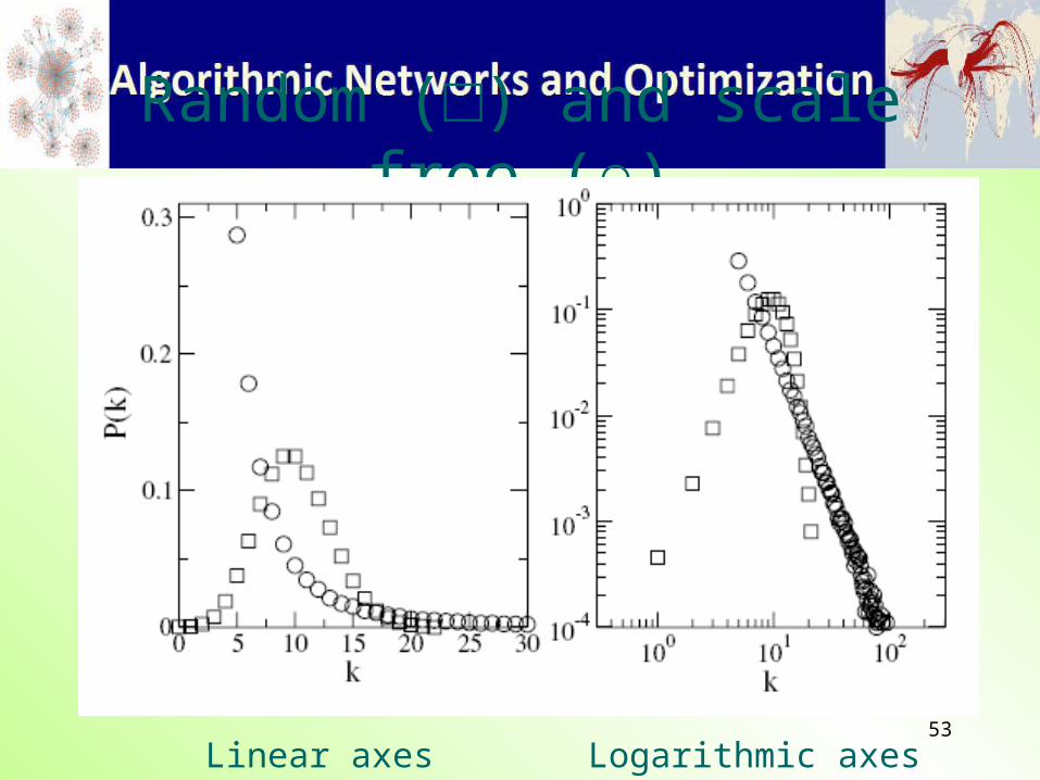
Random (□) and scale free (○)
Linear axes Logarithmic axes
54
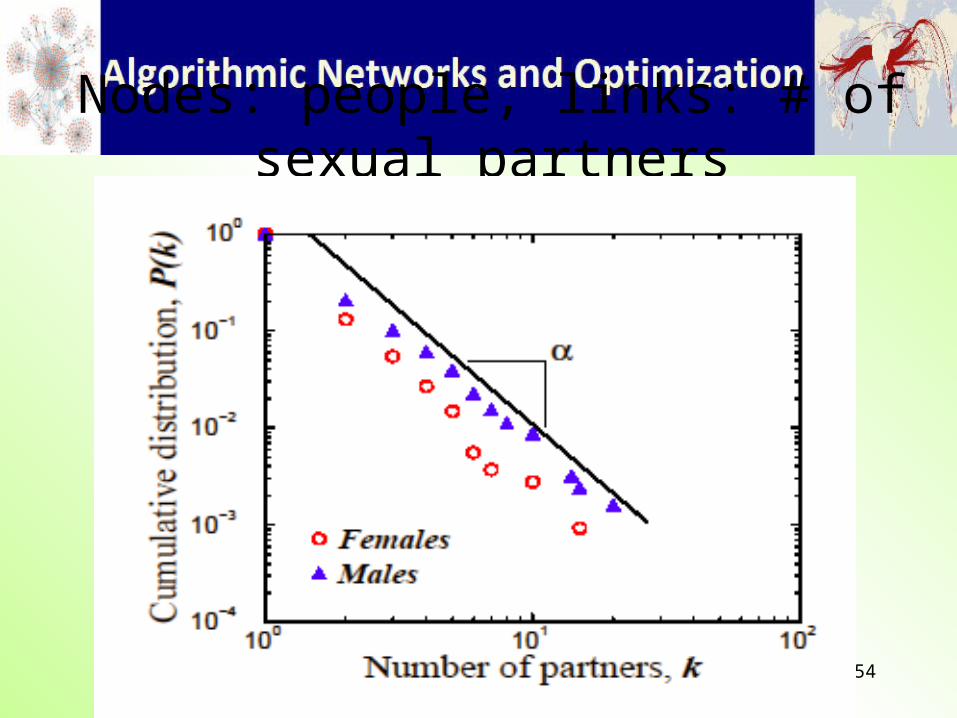
Nodes: people, links: # of sexual partners
55
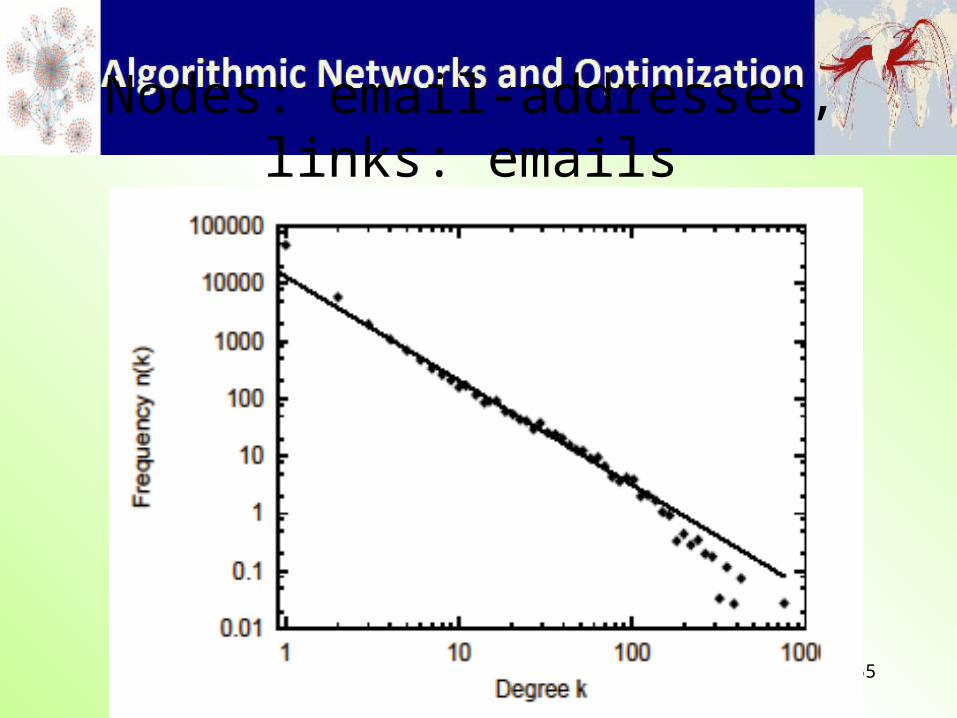
Nodes: email-addresses, links: emails
56
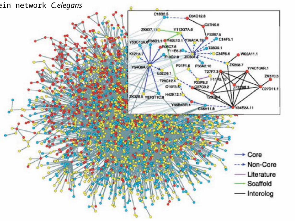
Protein network C.elegans
57
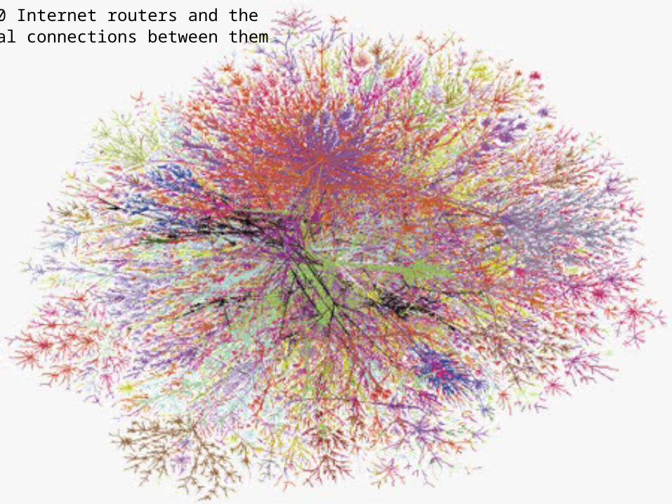
100 000 Internet routers and the physical connections between them
58
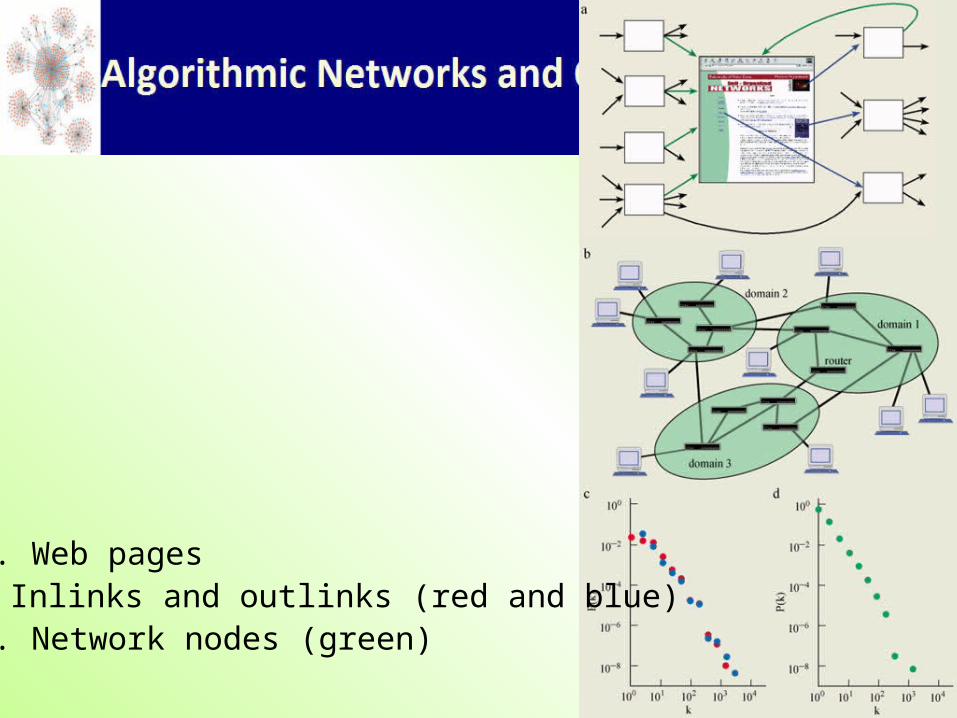
c. Web pages• Inlinks and outlinks (red and blue)d. Network nodes (green)
59
END LECTURE