1

The Identification of Scale-Free

Gene-Protein Networks

Ronald Westra

Department of Mathematics

Maastricht University

2

1. Biological background and problem formulation

2. Modeling of dynamic gene/proteins interactions

3. Scale-free network structures

4. Reconstruction of scale-free gene/proteins networks

5. Conclusions

Items in this Presentation

3

1. Biological background

Do gene-protein networks exhibit characteristic architectural and structural properties that may act as a format for reconstruction?

Some observations ...

4

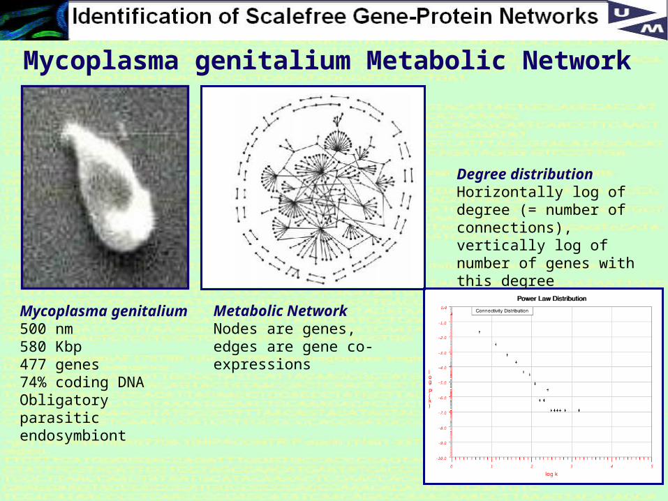
Mycoplasma genitalium500 nm580 Kbp477 genes74% coding DNAObligatory parasitic endosymbiont

Mycoplasma genitalium Metabolic Network

Metabolic NetworkNodes are genes, edges are gene co-expressions

Degree distributionHorizontally log of degree (= number of connections), vertically log of number of genes with this degree

5

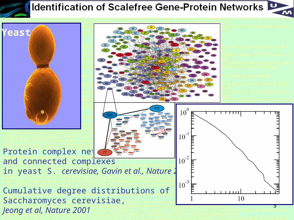
Protein complex networkand connected complexes in yeast S. cerevisiae, Gavin et al., Nature 2002.

Cumulative degree distributions of Saccharomyces cerevisiae, Jeong et al, Nature 2001

Yeast

6

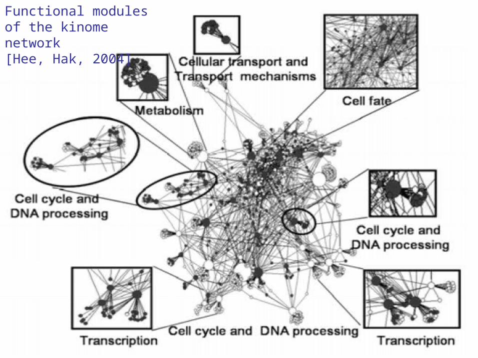
Functional modules of the kinome network [Hee, Hak, 2004]

7

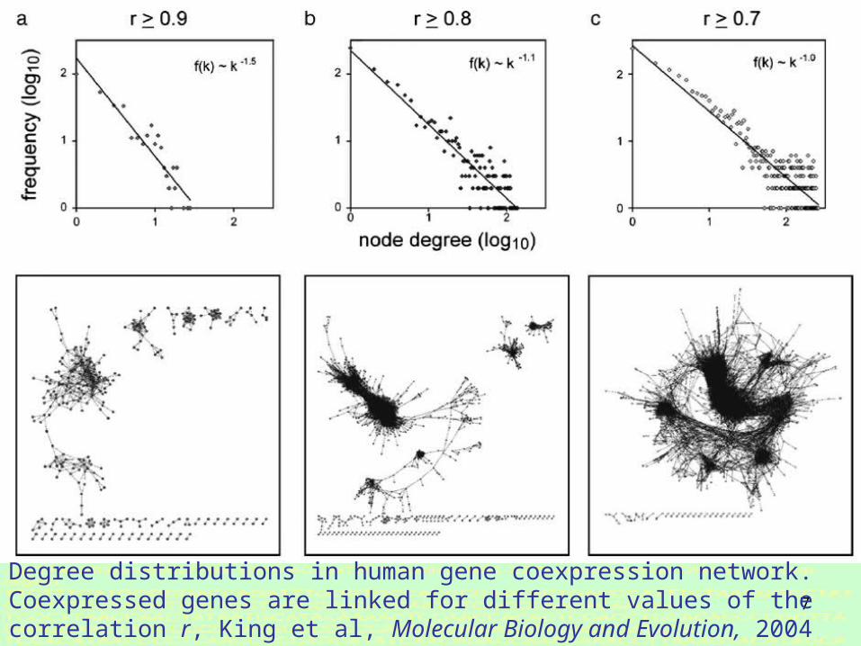
Degree distributions in human gene coexpression network. Coexpressed genes are linked for different values of the correlation r, King et al, Molecular Biology and Evolution, 2004

8

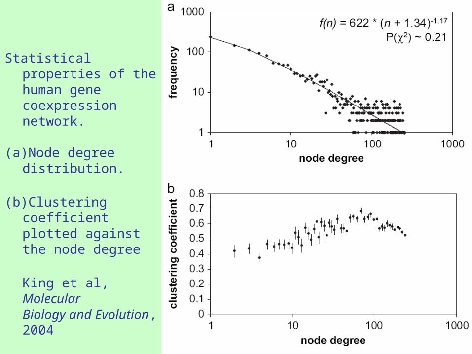
Statistical properties of the human gene coexpression network.

(a)Node degree distribution.

(b)Clustering coefficient plotted against the node degree

King et al, Molecular Biology and Evolution, 2004

9

Objective:

* Are there distinctive architectural properties in gene-protein networks that facilitate their reconstruction from experimental data? (it helps if you know how it looks like)

Example: sparsity (Yeung et al. 2003, etc)

* Are there other special network properties that work

similarly? Or even better?

Problem formulation

10

2. Modeling Interactions between Genes and Proteins

Prerequisite for the successful reconstruction of gene-protein networks is the way in which the dynamics of their interactions is modeled.

11

Components in Gene-Protein networks

Genes: ON/OFF-switches (→ continuous)

RNA&Proteins: vectors of information exchange between genes

External inputs: interact with higher-order proteins

12

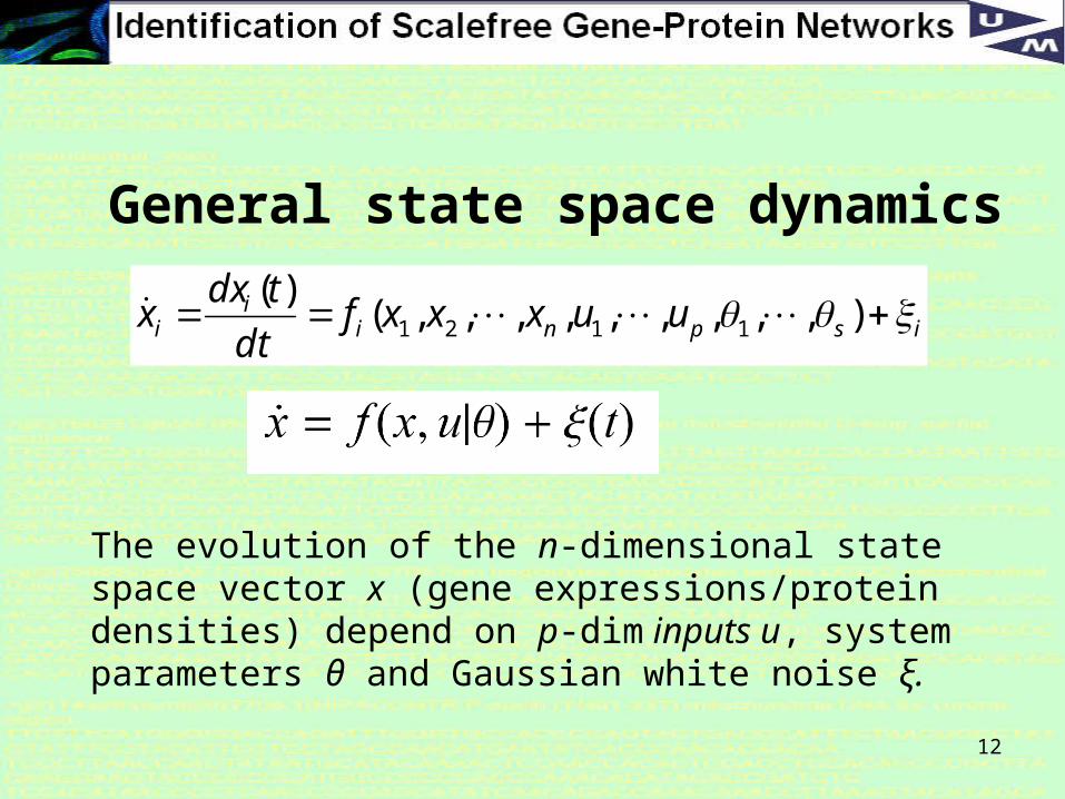
General state space dynamics

The evolution of the n-dimensional state space vector x (gene expressions/protein densities) depend on p-dim inputs u, system parameters θ and Gaussian white noise ξ.

ispnii

i uuxxxfdt

tdxx ),,,,,,,,,(

)(1121

13

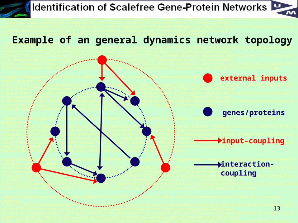
external inputs

input-coupling

genes/proteins

interaction-coupling

Example of an general dynamics network topology

14

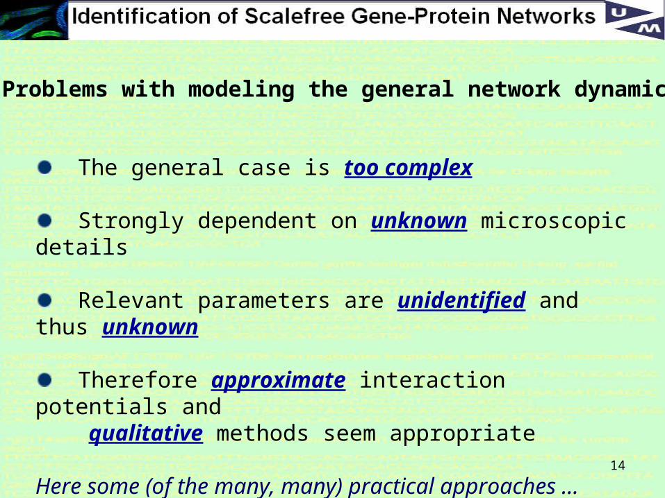
The general case is too complex

Strongly dependent on unknown microscopic details

Relevant parameters are unidentified and thus unknown

Therefore approximate interaction potentials and qualitative methods seem appropriate

Here some (of the many, many) practical approaches …

Problems with modeling the general network dynamics

15

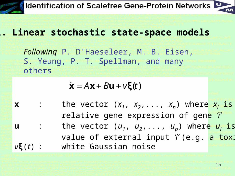
1. Linear stochastic state-space models

Following P. D'Haeseleer, M. B. Eisen, S. Yeung, P. T. Spellman, and many others

x : the vector (x1, x2,..., xn) where xi is the

relative gene expression of gene ‘í’u : the vector (u1, u2,..., up) where ui is the

value of external input ‘í’ (e.g. a toxic agent)νξ(t) : white Gaussian noise

)(tvBA ξuxx

16

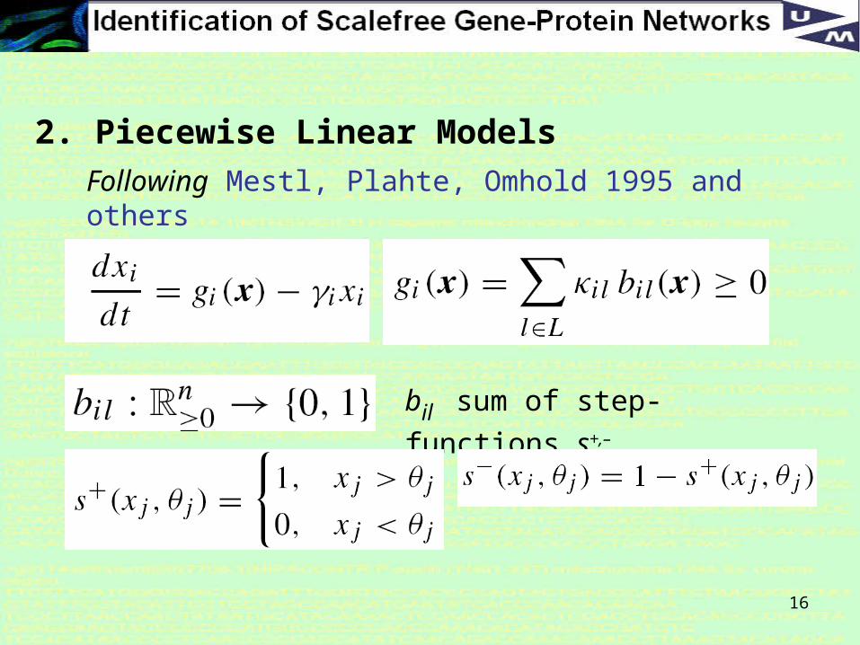
2. Piecewise Linear Models

Following Mestl, Plahte, Omhold 1995 and others

bil sum of step-functions s+,–

17

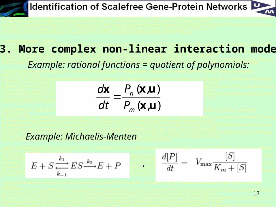
3. More complex non-linear interaction models

Example: rational functions = quotient of polynomials:

),(

),(

ux

uxx

m

n

P

P

dt

d

Example: Michaelis-Menten

→

18

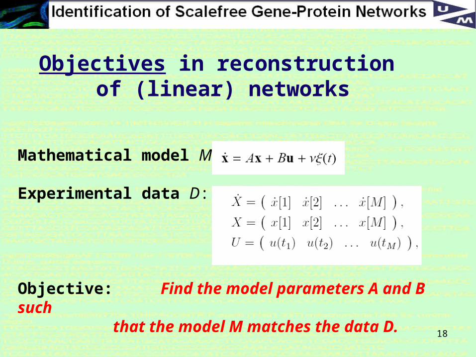
Objectives in reconstruction of (linear) networks

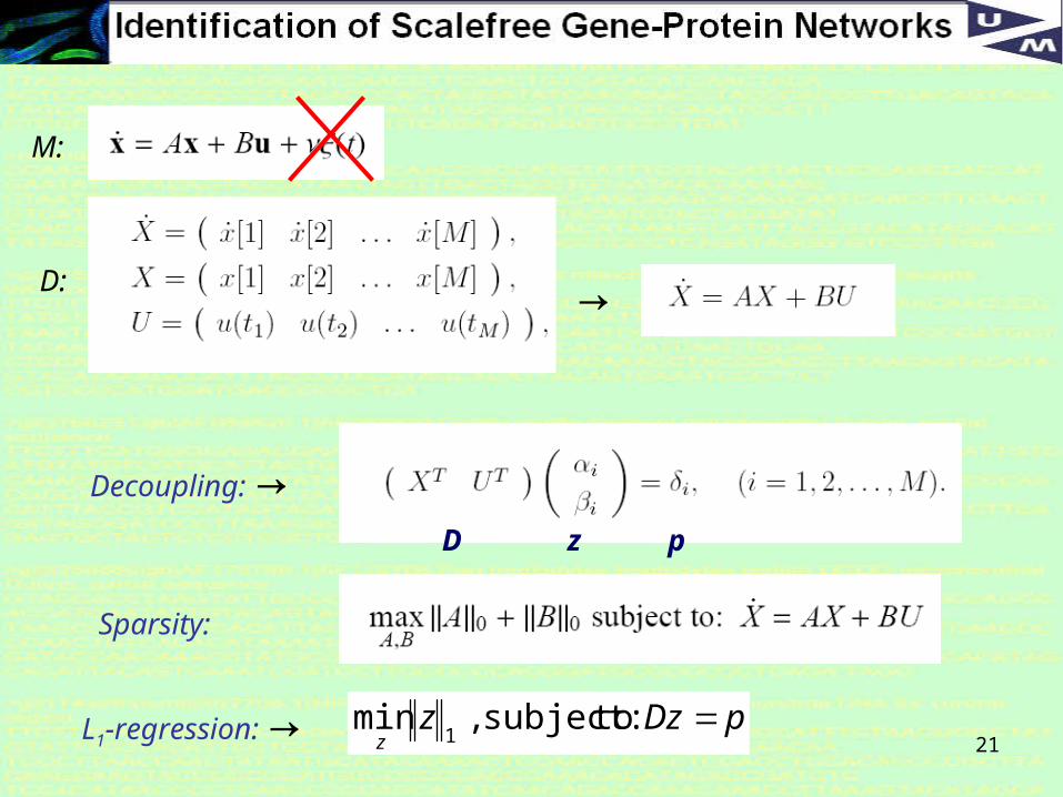
Mathematical model M:

Experimental data D:

Objective: Find the model parameters A and B suchthat the model M matches the data D.

19

Reconstruction of SPARSE LINEAR networks

In most cases the mathematical complexities in finding a realistic network structure are too severe

Therefore, some researchers have introduced new constraints that facilitate the computation

The best example is SPARSITY in a LINEAR network :

20

Major Problem in reconstruction of sparse networks

The system is severely under-constrained as there are typically far more model parameters A and B than there is experimental data D.

A useful trick is to assume that the system is heavily sparse and linear [Yeung et al, Guthke et al, …]

In that case the system can be: (i) decomposed row-for-row, and (ii) L1-regression can be employed

21

→

Decoupling: →

pDzzz

:tosubject,min1

Sparsity:

L1-regression: →

M:

D:

D z p

22

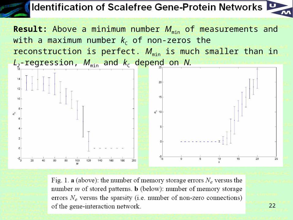
Result: Above a minimum number Mmin of measurements and with a maximum number kC of non-zeros the reconstruction is perfect. Mmin is much smaller than in L2-regression, Mmin and kC depend on N.

23

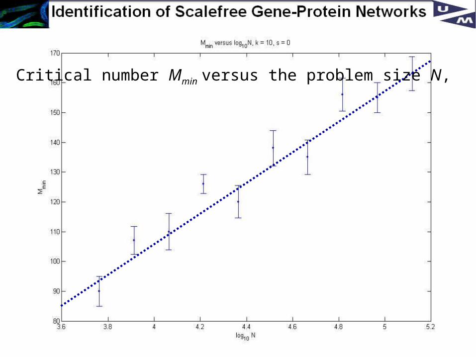
Critical number Mmin versus the problem size N,

24

3. Using special architectures of gene-protein networks

So far we used the fact that biological information processing networks mostly exhibit only a few connections (=sparse) and only a few genes and proteins control a considerable amount of all others (=hierarchic)

Other interesting properties of networks are also observed : regular, small world, scale free, exponential, apollonian, …

25

Network Architectures

There is more internal structure in a gene-protein network which we can use to derive more powerful constraints, and the most interseting is the Scale-Free (SF) property

26

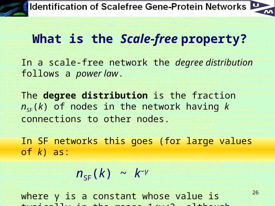
What is the Scale-free property?

In a scale-free network the degree distribution follows a power law.

The degree distribution is the fraction nSF(k) of nodes in the network having k connections to other nodes.

In SF networks this goes (for large values of k) as:

nSF(k) ~ k−γ

where γ is a constant whose value is typically in the range 1<γ<3, although occasionally it may lie outside these bounds.

27

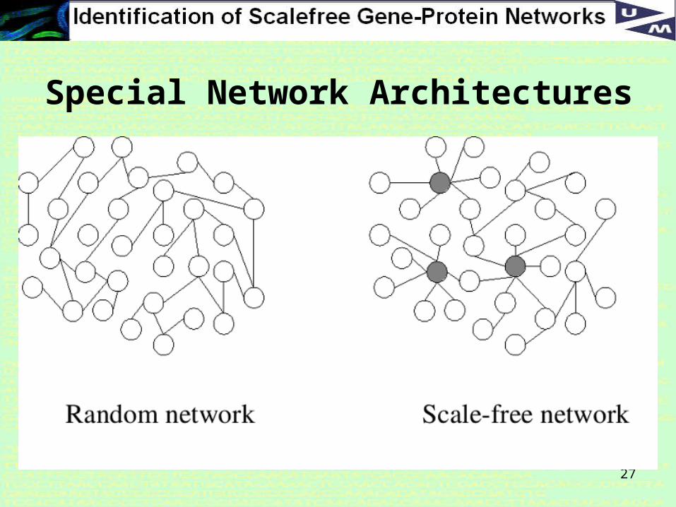
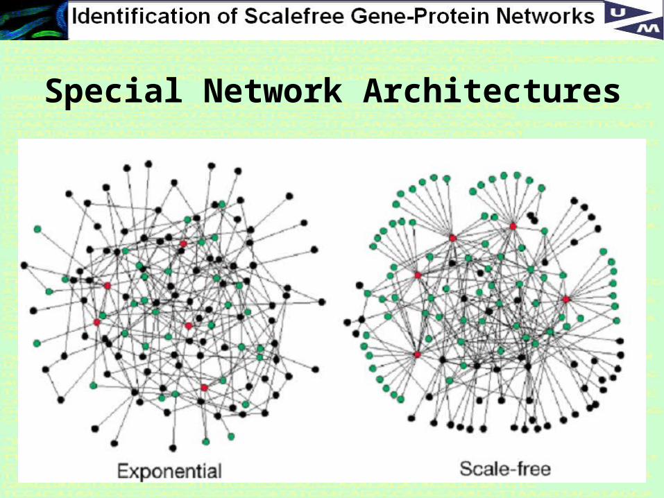
Special Network Architectures

28

Special Network Architectures

29

Why Scale-free?

Scale-free networks are noteworthy because many empirically observed networks appear to be scale-free, including the world wide web, protein networks, citation networks, and social networks.

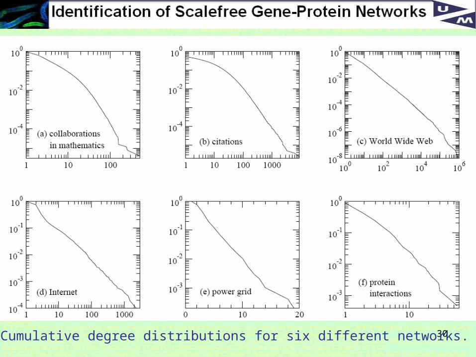
30Cumulative degree distributions for six different networks.

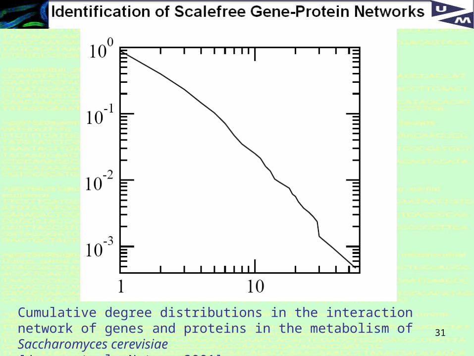
31

Cumulative degree distributions in the interaction network of genes and proteins in the metabolism of Saccharomyces cerevisiae [Jeong et al, Nature 2001]

32

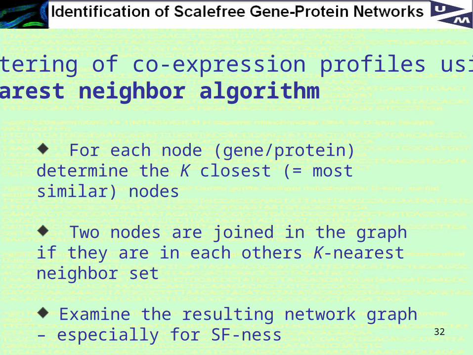
Clustering of co-expression profiles using K-nearest neighbor algorithm

For each node (gene/protein) determine the K closest (= most similar) nodes

Two nodes are joined in the graph if they are in each others K-nearest neighbor set

Examine the resulting network graph – especially for SF-ness

33

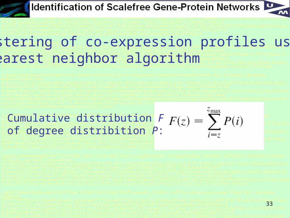
Clustering of co-expression profiles using K-nearest neighbor algorithm

Cumulative distribution F of degree distribition P:

34

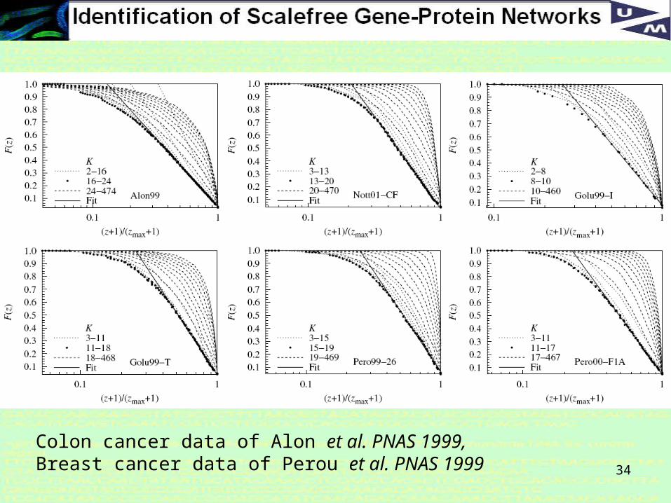
Colon cancer data of Alon et al. PNAS 1999, Breast cancer data of Perou et al. PNAS 1999

35

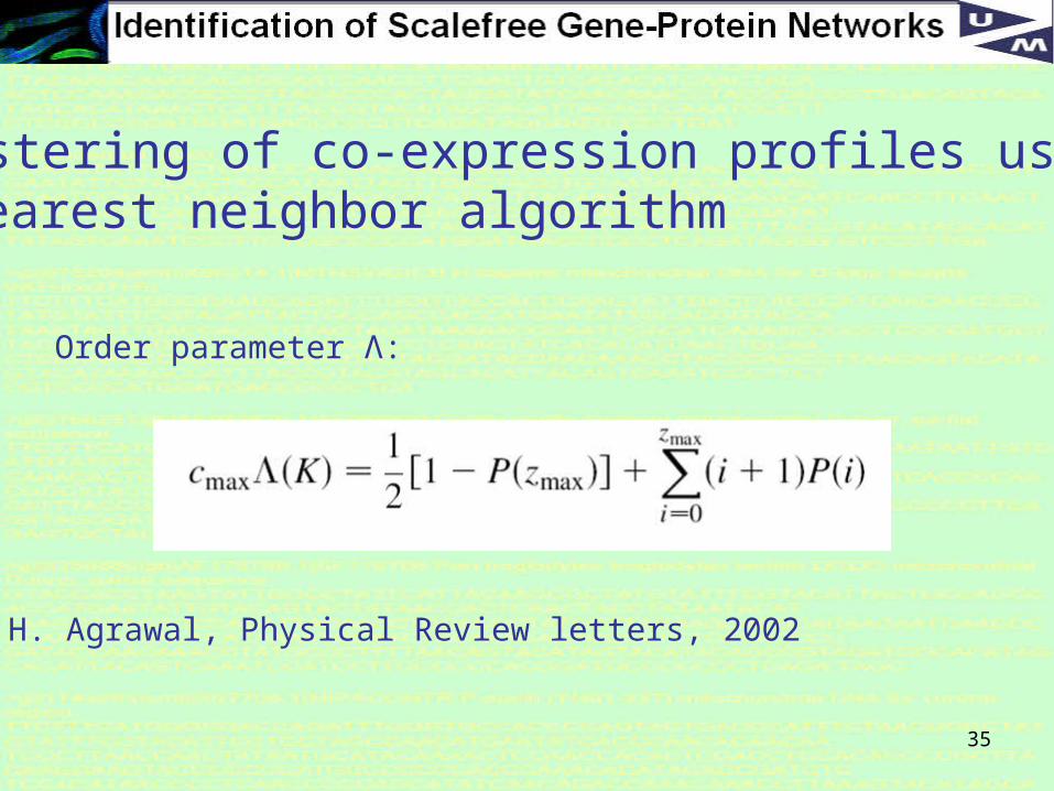
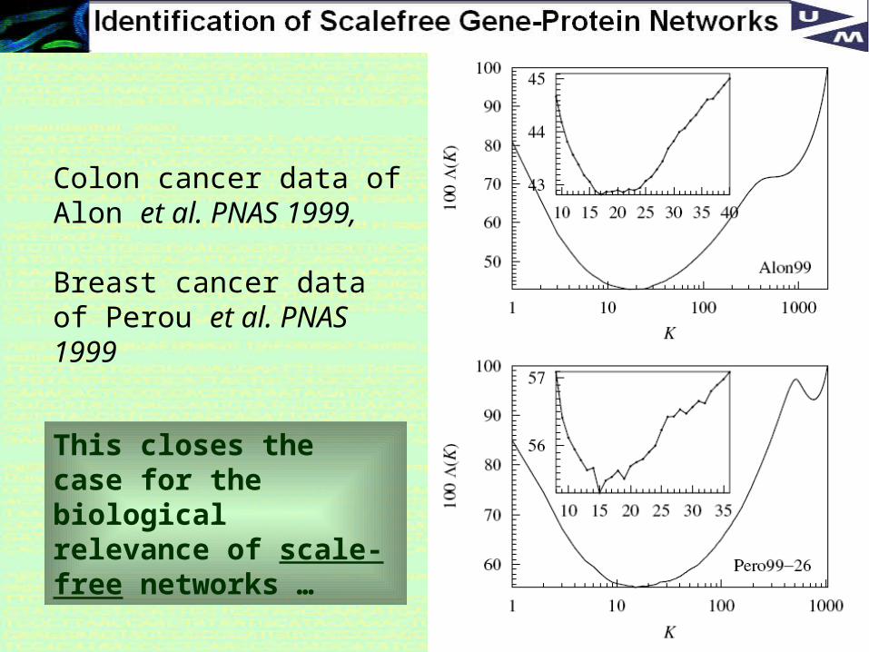
Order parameter Λ:

Clustering of co-expression profiles using K-nearest neighbor algorithm

H. Agrawal, Physical Review letters, 2002

36

Colon cancer data of Alon et al. PNAS 1999,

Breast cancer data of Perou et al. PNAS 1999

This closes the case for the biological relevance of scale-free networks …

37

CENTRAL THOUGHT

Conjecture:

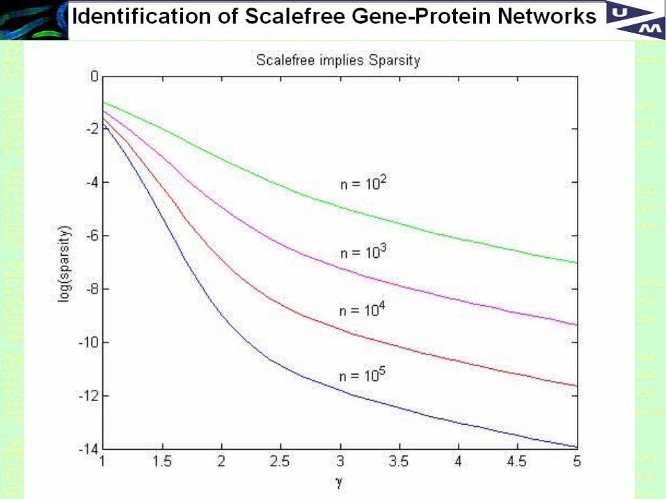
Scalefree-ness in a (gene regulatory) network implies sparsity.

SF is much stronger than sparsity … it also requires a specific distribution of connections in the network – and hence in the connectivity matrix, namely the SF powerlaw

Not only a large number of zeros are required, they are also grouped in a special manner.

38

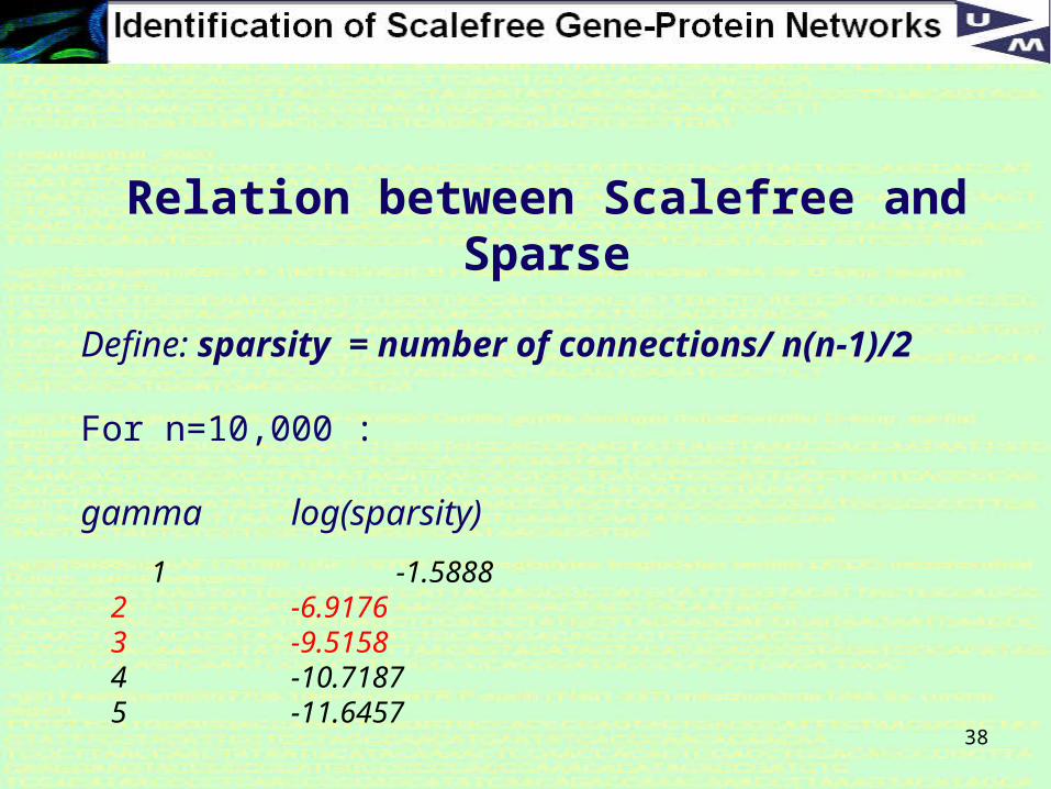
Relation between Scalefree and Sparse

Define: sparsity = number of connections/ n(n-1)/2

For n=10,000 :

gamma log(sparsity)

1 -1.5888 2 -6.9176 3 -9.5158 4 -10.7187 5 -11.6457

39

40

Reconstruction of scalefree networks

For these reasons, the reconstruction of networks using the SF-property should be much more effective than from sparse networks

41

Requirements

For the reconstruction of a scalefree (gene-protein) interaction system we need:

1. a suitable parametrised formal model

2. a method for optimising the scalefreeness of the system with respect to the model parameters for a given set of measurements (e.g. microarrays)

We will visit these items in the following slides ...

42

Philosophy:

The experimental data bounds the feasible parameter set A and B, and the scalefree-ness (SF) of A and B should be as high as possible consistent with the data D

4. Reconstruction of scalefree gene-protein networks

43

For simplicity we assume a non-symmetric, and SF gene/protein network with a linear state space dynamics

Suppose we have a set of M observations of genome-wide expression profiles (e.g. microarrays)

Linear Model of gene-protein networks

44

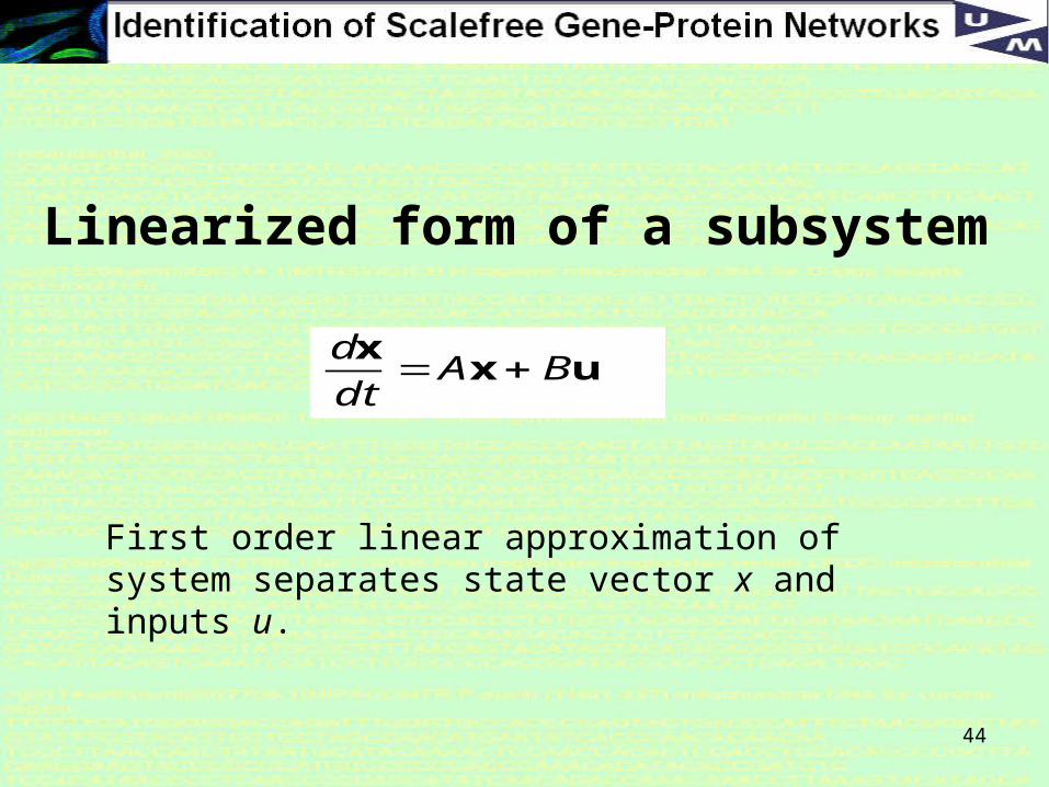
Linearized form of a subsystem

First order linear approximation of system separates state vector x and inputs u.

uxx

BAdt

d

45

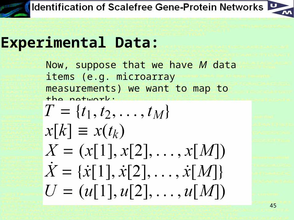
Experimental Data:

Now, suppose that we have M data items (e.g. microarray measurements) we want to map to the network:

46

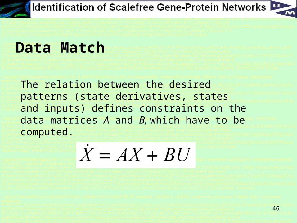
The relation between the desired patterns (state derivatives, states and inputs) defines constraints on the data matrices A and B, which have to be computed.

Data Match

47

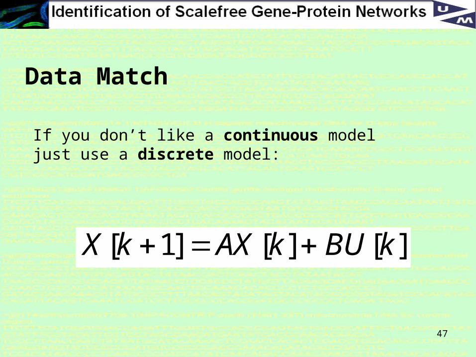
][][]1[ kBUkAXkX

If you don’t like a continuous model just use a discrete model:

Data Match

48

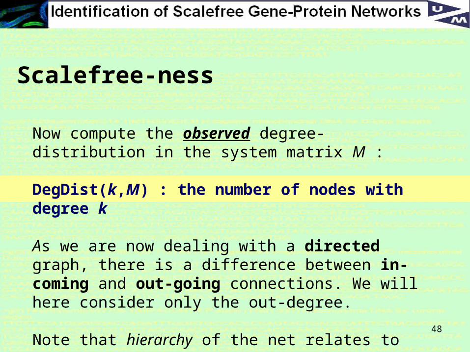
Now compute the observed degree-distribution in the system matrix M :

DegDist(k,M) : the number of nodes with degree k

As we are now dealing with a directed graph, there is a difference between in-coming and out-going connections. We will here consider only the out-degree.

Note that hierarchy of the net relates to the in-degree.

Scalefree-ness

49

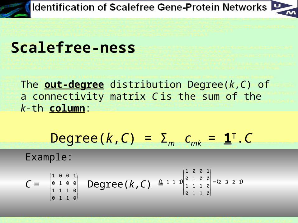
The out-degree distribution Degree(k,C) of a connectivity matrix C is the sum of the k-th column:

Degree(k,C) = Σm cmk = 1T.C

Scalefree-ness

1232

0110

0111

0010

1001

.1111

0110

0111

0010

1001

.

Example:

C = Degree(k,C) =

50

The degree is the basis for computing the degree distribution DegDist(k,C) of a connectivity matrix C. How can we determine the connectivity matrix for an arbitrary interaction matrix M like the matrices A and B in our linear model?

Answer: we approximate the connectivity matrix of M to an accuracy ε as Cε(M), similar to the approximation δε(x) of the δ-function δ(x) in measure theory …

Scalefree-ness

51

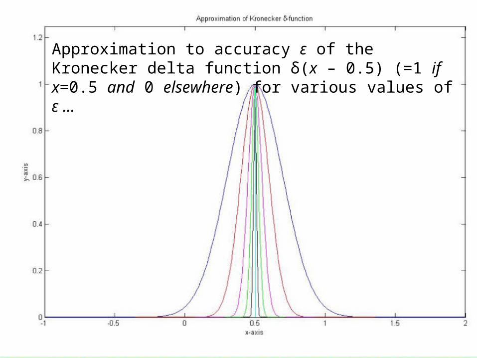
Approximation to accuracy ε of the Kronecker delta function δ(x – 0.5) (=1 if x=0.5 and 0 elsewhere) for various values of ε …

52

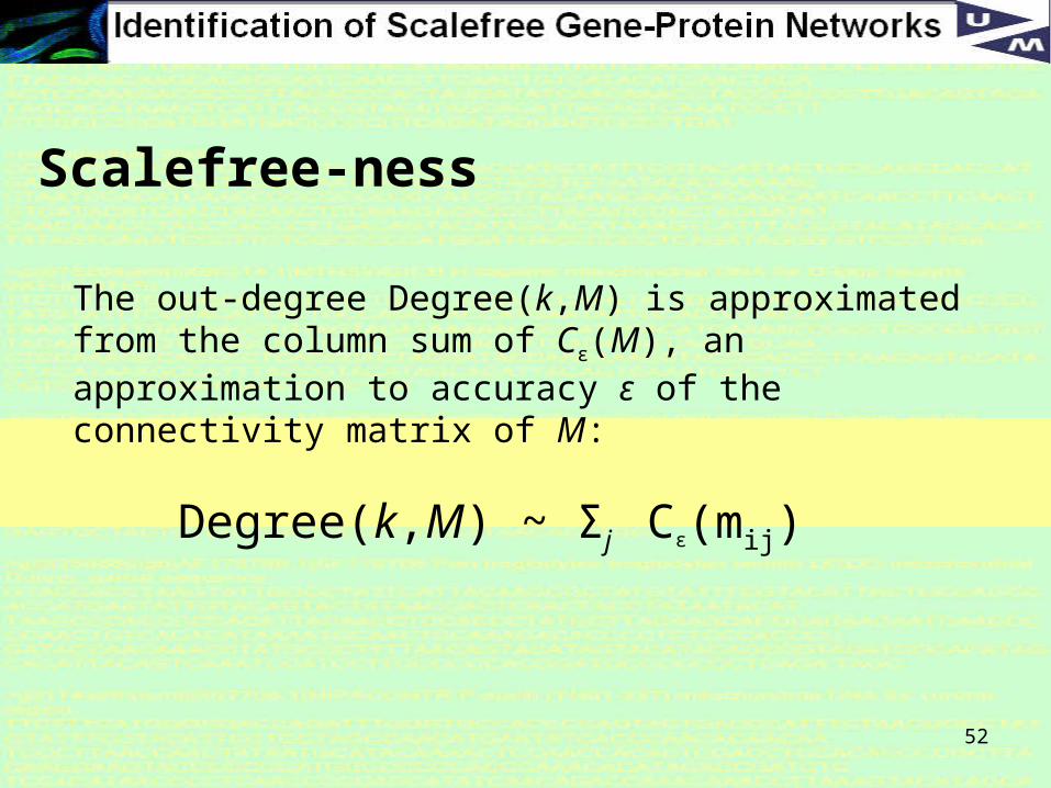
The out-degree Degree(k,M) is approximated from the column sum of Cε(M), an approximation to accuracy ε of the connectivity matrix of M:

Degree(k,M) ~ Σj Cε(mij)

Scalefree-ness

53

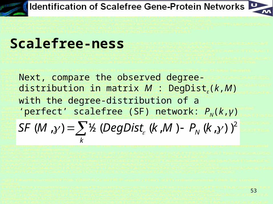
Next, compare the observed degree-distribution in matrix M : DegDistε(k,M) with the degree-distribution of a ‘perfect’ scalefree (SF) network: PN(k,γ) ~ k-γ

Scalefree-ness

k

N kPMkDegDistMSF 2) ),(),((½),(

54

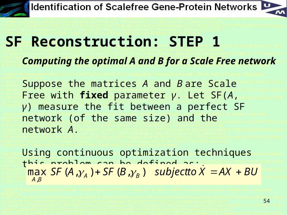
Computing the optimal A and B for a Scale Free network

Suppose the matrices A and B are Scale Free with fixed parameter γ. Let SF(A, γ) measure the fit between a perfect SF network (of the same size) and the network A.

Using continuous optimization techniques this problem can be defined as:

SF Reconstruction: STEP 1

BUAXXtosubjectBSFASF BABA

),(),(max,

55

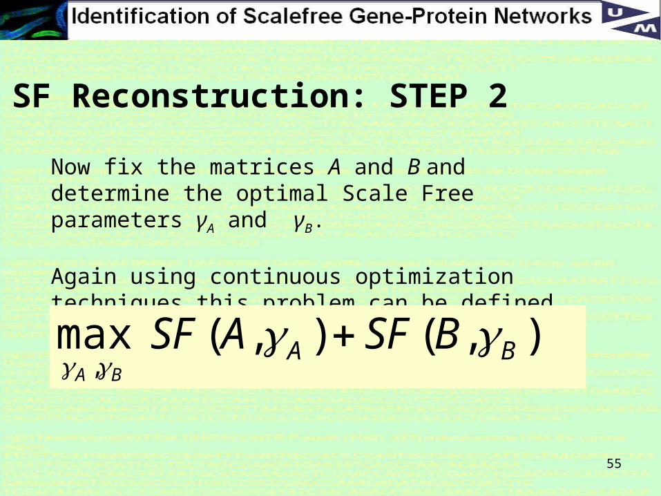
Now fix the matrices A and B and determine the optimal Scale Free parameters γA and γB.

Again using continuous optimization techniques this problem can be defined as:

SF Reconstruction: STEP 2

),(),(max,

BA BSFASFBA

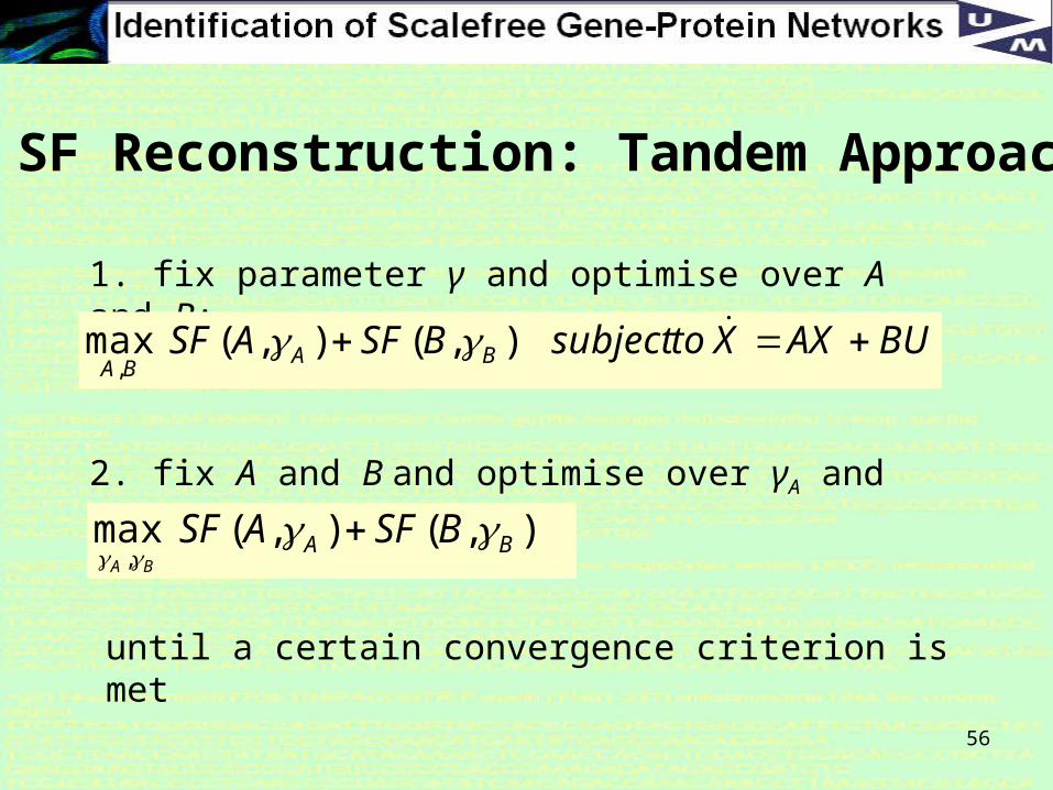
56

2. fix A and B and optimise over γA and γB:

SF Reconstruction: Tandem Approach

),(),(max,

BA BSFASFBA

1. fix parameter γ and optimise over A and B:

BUAXXtosubjectBSFASF BABA

),(),(max,

until a certain convergence criterion is met

57

Some results of comparing Sparse and SF reconstruction

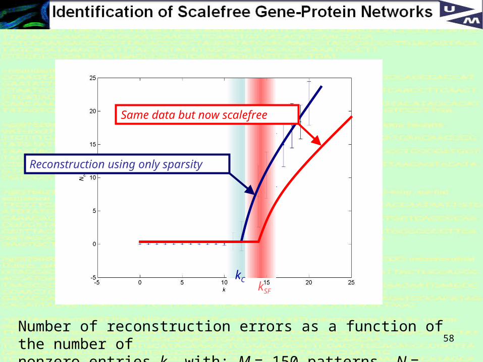
58Number of reconstruction errors as a function of the number of nonzero entries k, with: M = 150 patterns, N = 50000 genes.

kCkSF

Reconstruction using only sparsity

Same data but now scalefree

59

kC

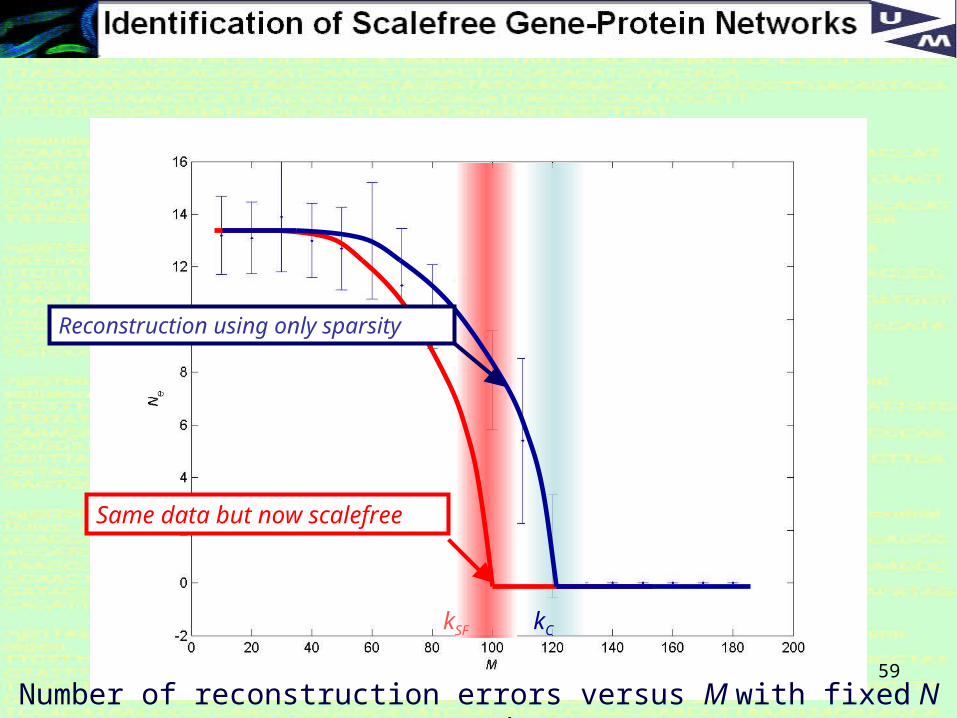
Number of reconstruction errors versus M with fixed N = 50000, k = 10.

Same data but now scalefree

kSF

Reconstruction using only sparsity

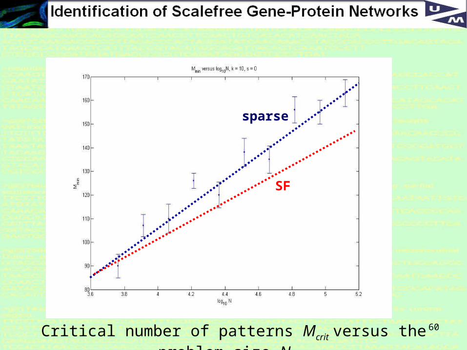
60Critical number of patterns Mcrit versus the problem size N,

sparse

SF

61

The system can not be decoupled as in sparse estimation (at least with L2-norm)

This means that the entire network has to be considered, resulting in long computation times.

If the underlying network is not scalefree this approach of course does not work

SF Reconstruction: Disadvantages

62

5. Conclusions

Assuming sparsity in linear time-invariant state space models for gene-protein networks allows for the effective network reconstruction using a small amount of data.

The scale-free property in networks implies network sparsity, and moreover requires a specific degree distribution. This is therefore a much stronger constraint than sparsity, and it is biologically plausible.

A mathematical tandem approach is able to fit a SF network architecture to observed data. The attractive computational properties of sparse identification however seem to be lost.

63

* Jeong, H., Mason, S., Barabasi, A.-L., and Oltvai, Z. N.,Lethality and centrality in protein networks, Nature 411, 41–42 (2001).

* Hee YK, Hak YK, Functional modules from protein networks of kinome and cell cycle in Saccharomyces cerevisiae, Proc. of IEEE Computational Systems Bioinformatics Conference (CSB), 2004.

* Jordan IK, Mariño-Ramírez L, Wolf YI, Koonin EV. Conservation and coevolution in the scale-free human gene coexpression network, Mol Biol Evol. 2004 Nov; 21(11):pp. 2058-70.

Some key references

64

Other members of the Computational Lifesciences Team

• Jordi Heijman (PhD student) 1,3• Stef Zeemering (PhD students) 1• Ralf Peeters 1• Goele Hollanders (PhD student) 1,2• Geert Jan Bex 2• Marc Gyssens 2• Yoram Rudy 3, 1 (visiting professor)

1: University of Maastricht, Dep.Mathematics (Netherlands): 2: University of Hasselt, Dep. Computer Science (Belgium): 3: Rudy Lab at Washington University (St. Louis USA)

65

66

Discussion …