Embed Size (px)
Citation preview
PHYS 652: Astrophysics 1
1 Lecture 1: Introduction, Outline and Motivation
“The most incomprehensible thing about the world is that it is comprehensible.”Albert Einstein
Astrophysics is the branch of astronomy that deals with the physics of the Universe, including thephysical properties (luminosity, density, temperature, chemical structure) of celestial objects suchas stars, galaxies and the interstellar medium, as well as their interactions. Astrophysics is a verybroad subject: it includes mechanics, statistical mechanics, thermodynamics, electromagnetism,relativity, particle physics, high energy physics, nuclear physics, and others.
Cosmology is theoretical astrophysics at its largest scales, where general relativity plays a majorrole. It deals with the Universe as a whole — its origin, distant past, evolution, structure. Whenlooking at the world at such grand scales, locally “flat” and “slow” approximation — the realm ofthe Newtonian mechanics — is no longer justified.
Because its subject matter involves such important and overarching questions, such as: ‘How didwe get here?’, ‘Was there a beginning?’, ‘Are we special?’, thus heavily flirting with philosophy andtheology, the modern cosmology has proven to be a dynamical battleground for competing ideas.In this arena where greatest scientific minds (and egos!) battled, we have many instances of drama,thrills, twists, and, of course, mystery:
• a priest-scientist breaking with the church cannons to interpret his solutions as having “a daywithout yesterday” (Fr. Georges Lemaıtre), a progenitor term to the “Big Bang”;
• one scientist’s mockery of the opposing camp’s view immortalized (term “Big Bang” wascoined by a steady-state theory proponent Fred Hoyle);
• a “fudge factor” introduced, then discarded in embarrassment, then later reintroduced as ouronly hope to get our cosmic books to balance (Einstein’s cosmological constant);
• the greatest experimental evidence for the Big Bang coming about by sheer accident! (cosmicmicrowave background radiation);
• finally, we are still searching for answers so as to what comprises about 96% of the content ofthe Universe. Over 70% of the mass-energy content of the Universe is in form of the unknownvacuum energy called “dark energy”. Over 80% of the mass is in the form of the mysterious“dark matter”.
Course Outline
This course will be composed of three parts:
1. General relativity as the foundation of cosmology
Overview of the basic concepts of the theory of general relativity (GR) and the formalism itprovides for studying the evolution of the Universe:
(a) Spacetime: time and space treated on equal footing.
(b) GR uses tools of differential geometry: metrics, covariant and contravariant tensors,invariants. When the equations of motion are written in tensor form, they are invariantunder metric transformation.
1
PHYS 652: Astrophysics 2
(c) Geodesic equation: how particles move in curved spacetime.
(d) Einstein’s equations: how matter curves spacetime.
(e) Solutions: Friedmann-Lemaıtre-Robertson-Walker Universe.
(f) The horizon problem leads to inflation theory. Inflation theory also explains the observedflatness of the Universe. De Sitter Universe.
2. Interpreting the Universe
Implications of solutions to Einstein’s equations:
(a) Brief history of time: from the Big Bang to present day.
(b) Cosmic Microwave Background (CMB) radiation.
(c) Dark matter: possible candidates and the current search.
3. Black holes, stars and galaxies:
(a) Black holes: singularities of Einstein’s equations.
(b) Stars: structure, evolution and mathematical models.
(c) Galaxies: classification, evolution and mathematical models.
Motivation: Newton vs. Einstein
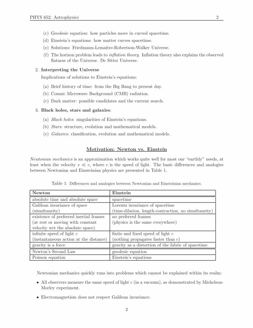
Newtonian mechanics is an approximation which works quite well for most our “earthly” needs, atleast when the velocity v ≪ c, where c is the speed of light. The basic differences and analogiesbetween Newtonian and Einsteinian physics are presented in Table 1.
Table 1: Differences and analogies between Newtonian and Einsteinian mechanics.
Newton Einstein
absolute time and absolute space spacetime
Galilean invariance of space Lorentz invariance of spacetime(simultaneity) (time-dilation, length-contraction, no simultaneity)
existence of preferred inertial frames no preferred frames(at rest or moving with constant (physics is the same everywhere)velocity wrt the absolute space)
infinite speed of light c finite and fixed speed of light c(instantaneous action at the distance) (nothing propagates faster than c)
gravity is a force gravity as a distortion of the fabric of spacetime
Newton’s Second Law geodesic equation
Poisson equation Einstein’s equations
Newtonian mechanics quickly runs into problems which cannot be explained within its realm:
• All observers measure the same speed of light c (in a vacuum), as demonstrated by Michelson-Morley experiment.
• Electromagnetism does not respect Galilean invariance.
2
PHYS 652: Astrophysics 3
• Why do all bodies experience the same acceleration regardless of their mass, i.e., why is theinertial and gravitational mass the same (as measured experimentally throughout history)?
Einstein’s theory of special relativity (SR) introduced some revolutionary concepts:
• “Abolished” absolute time — introduced 4D spacetime as an inseparable entity.
• Finite and fixed speed of light c.
• Established equivalence between energy and mass (massless photons are subject to gravity).
• However, the 4D spacetime considered in SR is still flat — Minkowski metric.
Einstein’s theory of general relativity continued the revolution:
• Equivalence principle: Established equivalence between the inertial and gravitational mass.
• Cosmological principle: Our position is “as mundane as it can be” (on large spatial scales,the Universe is homogeneous and isotropic).
• Relativity: Laws of physics are the same everywhere.
• New definition of gravity: Gravity is the distortion of the structure of spacetime as caused bythe presence of matter and energy. The paths followed by matter and energy in spacetime aregoverned by the structure of spacetime. This great feedback loop is described by Einstein’sfield equations. So, the 4D spacetime considered in GR is no longer flat.
After establishing GR as the way to describe the Universe and learning its mathematical formal-ism, we will finally embark on a journey of expressing mathematically the world around us on largestscales, physically interpreting the implications and reconciling them with the the observations.
Many of the phenomena for which we now have overwhelming evidence — the Big Bang, ex-panding Universe, CMB radiation, black holes, among others — have been first predicted by thesolutions of Einstein’s equations. Therefore, it is the mathematics that holds the keys to unlockingthe mysteries of the Universe, so let us begin acquiring required mathematical skills!
3
PHYS 652: Astrophysics 4
2 Lecture 2: Basic Concepts of General Relativity
“Everything should be made as simple as possible, but not simpler.”Albert Einstein
The Big Picture: Today we are going to introduce the notation used in GR, define the metric,compare motion in flat and curved metrics and derive the geodesic equation — an equivalent toNewton’s Second Law in curved spacetime.
Notation
4-vector: (t, x, y, z) → (x0, x1, x2, x3).
Indices convention:
• Roman letters (i, j, k, l,m, n) run from 1 to 3;
• Greek letters (α, β, γ, δ, µ, ν, η, ξ) run from 0 to 3.
Einstein summation (summation over repeated indices): v′α =∑3
β=0∂x′α
∂xβvβ ≡ ∂x′α
∂xβvβ .
Contravariant vector transforms as A′α = ∂x′α
∂xβAβ (index is a superscript).
Covariant vector transforms as A′α = ∂xβ
∂x′αAβ (index is a subscript).
Tensors: objects with multiple indices.
First rank (one index):
• contravariant: A′α = ∂x′α
∂xβAβ.
• covariant: A′α = ∂xβ
∂x′αAβ .
Second rank (two indices):
• contravariant: A′αβ = ∂x′α
∂xξ∂x′β
∂xν Aξν .
• covariant: A′αβ = ∂xα
∂x′ξ∂xβ
∂x′ν Aξν .
• mixed: A′αβ = ∂x′α
∂xξ∂xν
∂x′βAξν .
N th rank (N indices):
• mixed: A′α1...αsαs+1...αN
= ∂x′α1
∂xβ1...∂x
′αs
∂xβs∂xαs+1
∂x′βs+1... ∂x
αN
∂x′βNAβ1...βsβs+1...βN
.
Operations with tensors:
• Addition: Aαβξν +Bαβξν = Cαβ
ξν .
• Subtraction: Aαβξν −Bαβkl = Dαβ
ξν .
• Tensor product: Aαβξν Bγδηψ = Gαβγδ
ξνηψ .
• Contraction: Aαββγ = Hαγ (summed over β).
• Inner product: Aαβξν Bνγδη = Pαβνγ
ξνδη = Kαβγξδη .
Importance: When written in tensor form, the equations of motion are invariant underappropriately defined transformation:
• Newtonian mechanics: 3-vector (x1, x2, x3) is invariant under Galilean transforma-tion.
4
PHYS 652: Astrophysics 5
• SR: 4-vector (x0, x1, x2, x3) is invariant under Lorentz transformation.
• GR: 4-vector (x0, x1, x2, x3) is invariant under general metric transformation.
Invariants: scalars which are the same in all coordinate systems.
Constants: we adopt a convention c = kB = G = ~ = 1 (to remain consistent with the book, andalso because many textbooks and papers employ these units).
Metric Tensors
Flat Euclidian space. Our common sense has taught us to think in terms of a flat space metric(Euclidian), where parallel lines never cross and angles in a triangle always sum up to 180o, thusstrongly reinforcing our Newtonian (incorrect!) notion of absolute space. In this formulation, theinvariant line element in Cartesian coordinates of space (x1, x2, x3) is:
ds2 = (dx1)2 + (dx2)2 + (dx3)2, (1)
and space is assumed to be flat. Another way to write this is
ds2 = δijdxidxj , (2)
where δαν is the Kronecker delta function (δαν = 1 if α = ν, δαν = 0 otherwise). Therefore, theEuclidian flat space metric tensor for Cartesian coordinates is given by:
δij =
1 0 00 1 00 0 1
. (3)
Invariant line element in an arbitrary coordinate system in flat space can be written in terms ofCartesian coordinates (change of variables) as:
ds2 = δijdxidxj = δij
∂xi
∂x′k∂xj
∂x′ldx′kdx′l ≡ pkldx
′kdx′l, (4)
where pkl is the space metric of the new coordinate system.Since the indices of the metric tensor enter the eq. (4) in an identical fashion, the metric tensor
is always symmetric. Furthermore, isotropy and homogeneity (as assumed in the flat Euclidianspace) implies that the metric tensor in such a space will necessarily be diagonal.
Flat Minkowski spacetime. We can now generalize this to 4-vectors in flat spacetime (x0, x1, x2, x3):
ds2 = ηαβdxαdxβ, (5)
where ηαβ is the Minkowski (flat) spacetime metric tensor
ηαβ =
−1 0 0 00 1 0 00 0 1 00 0 0 1
. (6)
Again, isotropy and homogeneity of spacetime leads to a diagonal metric tensor.
5
PHYS 652: Astrophysics 6
Curved spacetime. For a general (possibly curved) covariant spacetime metric tensor gαβ , theinvariant line element is given by
ds2 = gαβdxαdxβ, (7)
The contravariant spacetime metric tensor is simply a reciprocal of the covariant tensor gαβ :
gαβgβν = δαν . (8)
This implies that whenever the metric tensor is diagonal gαβ = (gαβ)−1.
One can take inner products of tensors with the metric tensor, thus lowering or raising indices:
Aαβ = gανAνβ , Aαβ = gανAβν . (9)
Expanding flat spacetime (Friedman-Lemaıtre-Robertson-Walker metric tensor).The metric tensor for a flat, homogeneous and isotropic spacetime which is expanding in its spatialcoordinates by a scale factor a(t) is obtained from the Minkowski metric by scaling the spatialcoordinates by a2(t):
gαβ =
−1 0 0 00 a2(t) 0 00 0 a2(t) 00 0 0 a2(t)
. (10)
Covariant Derivative
Consider a vector ~A given in terms of its components along the basis vectors:
~A = Aαeα. (11)
Differentiating the vector ~A using the Leibniz rule (fg)′ = f ′g + g′f , we obtain
∂ ~A
∂xα=
∂
∂xα
(
Aβ eβ
)
=∂Aβ
∂xαeβ +Aβ
∂eβ∂xα
. (12)
In flat Cartesian coordinates, the basis vectors are constant, so the last term in the equation abovevanishes. However, this is not the case in general curved spaces. In general, the derivative in thelast term will not vanish, and it will itself be given in terms of the original basis vectors:
∂eβ∂xα
= Γναβ eν . (13)
Γναβ is called the Christoffel symbol (or affine connection). It is given in terms of a metric:
Γναβ ≡ 1
2gνγ (gαγ,β + gγβ,α − gαβ,γ) . (14)
Taking the curvature of the ambient manifold into account when taking derivatives of vectorsor tensors yields covariant derivative:
Aα;β ≡ Aα,β − ΓναβAν , (15)
Aα;β ≡ Aα,β + ΓναβAν , (16)
where Aα,β ≡ ∂Aα
∂xβand Aα,β ≡ ∂Aα
∂xβ.
6

PHYS 652: Astrophysics 7
For vectors Aα and Aα defined along a curve xβ = xβ(s), the covariant derivative along thiscurve are
DAα
Ds≡ dAα
ds+ Γαβγ
dxγ
dsAβ,
DAαDs
≡ dAαds
− Γβαγdxγ
dsAβ. (17)
Covariant derivative is a curved spacetime analog of the ordinary derivative in Cartesian coordinatesin flat spacetime.
Principle of General Covariance states that all tensor equations valid in SR will also be validin GR if:
• the Minkowski metric ηαβ is replaced by a general curved metric gαβ ;
• all partial derivatives are replaced by covariant derivatives (,→;).
Examples:
dτ2 = −ηαβdxαdxβ =⇒ dτ2 = −gαβdx
αdxβ ,
ηαβuαuβ = −1 =⇒ gαβu
αuβ = −1
Tαβ,β = 0 =⇒ Tαβ;β = 0
Geodesic Equation
In Newtonian mechanics, the Second Law states that the forces impart acceleration on the bodyit acts on:
md2~x
dt2= ~F = −~∇Φ =⇒ d2~x
dt2= − 1
m~∇Φ. (18)
In the absence of forces acting on a body, the Second Law reduces to the First Law:
d2~x
dt2= 0. (19)
In flat Euclidian space and flat Minkowski spacetime, this also leads to straight lines.It is a fundamental assumption of GR that, in curved spacetimes, free particles (i.e., particles
feeling no non-gravitational effects) follow paths that extremize their proper interval ds. Such pathsare called geodesics. Therefore, generalizing Newton’s laws on motion of a particle in the absenceof forces (eq. (19)) to a general curved spacetime metric leads to the geodesic equation.
Important note: Here we derive the geodesic equation using the variational principle (Lagrange’sequations). This is an alternative to the approach presented in the textbook. Both approaches arepresented to provide a more thorough understanding — therefore they should both be studied andunderstood.
Suppose the points xi lie on a curve parametrized by the parameter λ, i.e.,
xα ≡ xα(λ), dxα =dxα
dλdλ, (20)
and the distance between two points A and B is given by
sAB =
∫ B
Ads =
∫ B
A
ds
dλdλ =
∫ B
A
√
gαβdxα
dλ
dxβ
dλdλ. (21)
7
PHYS 652: Astrophysics 8
The shortest path between the points A and B is called the geodesic, and it is found by extremizing(minimizing) the path sAB. This is done by standard tools of variational calculus which lead toLagrange equations, which we derive here as a reminder.
Extremizing the functional using a variational principle (Lagrange’s equations).Consider
G ≡∫ B
AL
(
λ, x,dx
dλ
)
dλ. (22)
Let x = X(λ) be the curve extremizing G. Then a nearby curve passing through A and B can beparametrized as x = X(λ) + εη(λ), such that η(A) = η(B) = 0. Extremizing eq. (22) we have:
dG
dε
∣
∣
∣
∣
ε=0
=
∫ B
A
(
∂L
∂xη +
∂L
∂xη
)
dλ where x ≡ dx
dλ, η ≡ dη
dλ
=
∫ B
A
∂L
∂xηdλ+
∫ B
A
∂L
∂xηdλ Now integrate by parts
=
∫ B
A
∂L
∂xηdλ+
∂L
∂xη|BA −
∫ B
A
d
dλ
∂L
∂xηdλ
=
∫ B
Aη
[
∂L
∂x− d
dλ
∂L
∂x
]
dλ = 0 Recall : η(A) = η(B) = 0 (23)
But the function η is arbitrary, so in order to have dGdε
∣
∣
ε=0, the bracket in the integrand must
vanish, and so we arrive at Lagrange’s equations:
∂L
∂x− d
dλ
∂L
∂x= 0, (24)
which can be extended to any number of phase-space coordinates:
∂L
∂xα− d
dλ
∂L
∂xα= 0. (25)
After this little side-derivation, let us march on toward the geodesic equation. We can nowapply the Lagrange’s equations to eq. (21), after using
L =1
2gγδx
γ xδ. (26)
(Alternatively, one can a more traditional form for the Lagrangian: L =√
gγδxγxδ, but mathe-matics is a lot cleaner with this choice).
After substituting eq. (26) into the eq. (25) we have
1
2gγδ,αx
γxδ − d
dλ[gγαx
γ ] = 0, (27)
where gγδ,α ≡ ∂gγδ∂xα . After recognizing that
d
dλgγα =
∂gγα∂xδ
xδ, (28)
we obtain
1
2gγδ,αx
γxδ − gγα,δxδxγ − gγαx
γ =(
1
2gγδ,α − gγα,δ
)
xγxδ − gγαxγ = 0.
8
PHYS 652: Astrophysics 9
Multiplying by gνα, the equation simplifies to
gνα(
1
2gγδ,α − gγα,δ
)
xγ xδ − xν = 0. (29)
Recasting it to a form resembling Newton’s laws, the eq. (29) it becomes
xν = −gνα(
gγα,δ −1
2gγδ,α
)
xγ xδ, (30)
or in terms of the Christoffel symbol Γνγδ:
xν = −Γνγδxγ xδ, (31)
(Note that going from the eq. (30) to the eq. (14), we have used that gγα,δxγxδ = gαδ,γ x
γxδ.)In Euclidian space and Minkowski spacetime, gαβ is diagonal and constant so its derivatives, andconsequently the Christoffel symbol vanish, thus leaving us with straight lines, as it should.
Another advantage for using the Lagrangian in the form given in eq. (26) is that solving theLagrange equation in (25) in each coordinate yields the differential equation of the same form asthe geodesic equation in (31). The Christoffel symbols can then simply be read off.
Recovering Newtonian gravity. Let us verify that in the limit of slow motion (v ≪ c) andweak, stationary gravitational fields, the geodesic equation yields Newton’s Second Law.
The limit of slow motion leads to the RHS of the eq. (31) to reduce only to Γν00(x0)2. But
Γν00 =1
2gνα (g0α,0 + gα0,0 − g00,α) = −1
2gναg00,α = −1
2gνig00,i (32)
because the stationary field approximation renders all gαβ,0 = 0. Using perturbation theory, recastthe metric as a small deviation from a Minkowski flat spacetime:
gαβ = ηαβ + ǫαβ, gαβ = ηαβ − ǫαβ, (33)
where ǫαβ is a small perturbation. Then, to the first order in ǫαβ :
Γν00 = −1
2
(
ηνi − ǫνi)
ǫ00,i = −1
2ηνiǫ00,i +O(ǫ2). (34)
Then Γ000 = 0 and Γj00 = −1
2ηjiǫ00,i. For ν = 0, x0 = d2t
d2λ= 0 and dt
dλ = const., and for ν = j
xj =d2xi
d2λ=
1
2ηjiǫ00,i(x
0)2 =1
2ηjiǫ00,i
(
dt
dλ
)2
. (35)
Butdxj
dλ=
dt
dλ
dxj
dt=⇒ xj =
d2xj
dλ2=
(
dt
dλ
)2 d2xj
dt2=⇒ d2xj
dt2=
1
2ηjiǫ00,i. (36)
Recalling that xj =(
xc ,
yc ,
zc
)
, and casting it in vector format we arrive to
d2~x
dt2=
1
2c2~∇ǫ00. (37)
When we compare this to Newton’s Second Law
d2~x
dt2= −~∇Φ, (38)
9
PHYS 652: Astrophysics 10
we find that ǫ00 = −2Φc2 and
g00 = −(
1 +2Φ
c2
)
. (39)
In spherical symmetry Φ = −GMr , so g00 = −
(
1 + 2GMrc2
)
. This quantifies how mass curves thespacetime in the Newtonian approximation.
10
PHYS 652: Astrophysics 11
3 Lecture 3: Einstein’s Field Equations
“God used beautiful mathematics in creating the world.”Paul Dirac
The Big Picture: Last time we derived the geodesic equation (a GR equivalent of Newton’sSecond Law), which describes how a particle moves in a curved spacetime. Today we are goingto derive the second part necessary to complete the dynamical description: how the presence ofmatter and energy curves the ambient spacetime. This is given by Einstein’s field equation, whichis nothing else but the GR analog of the Poisson equation.
Riemann Tensor, Ricci Tensor, Ricci Scalar, Einstein Tensor
Riemann (curvature) tensor plays an important role in specifying the geometrical propertiesof spacetime. It is defined in terms of Christoffel symbols:
Rαβγδ ≡ Γαβδ,γ − Γαβγ,δ + ΓνβδΓ
ανγ − ΓνβγΓ
ανδ, (40)
where Γαβδ,γ ≡ ∂∂xγ Γ
αβδ . The spacetime is considered flat if the Riemann tensor vanishes everywhere.
Riemann tensor can also be written directly in terms of the spacetime metric
Rαβγδ ≡1
2(gβγ,αδ + gαδ,βγ − gβδ,αγ − gαγ,βδ) + gµνΓ
ναγΓ
µβδ − gµνΓ
ναδΓ
µβγ (41)
thus revealing symmetries of the Riemann tensor:
Rαβγδ = −Rβαγδ = −Rαβδγ = Rγδαβ (42)
Rαβγδ + Rβδαγ +Rαδβγ = 0. (43)
Because of the symmetries above, the Riemann tensor in 4-dimensional spacetime has only 20independent components. The general rule for computing the number of independent componentsis an N -dimensional spacetime is N2(N2 − 1)/12.Ricci tensor is obtained from the Riemann tensor by simply contracting over two of the indices:
Rαβ ≡ Rγαγβ . (44)
It is symmetric, which means that it has at most 10 independent quantities.Ricci scalar is obtained by contracting the Ricci tensor over the remaining two indices:
R ≡ gαβRαβ = Rαα. (45)
Bianchi identities are another important symmetry of the Riemann tensor
Rαβγδ;ν +Rβανγ;δ +Rαβδν;γ = 0, (46)
which, after contracting, leads to
Rαβ;α =
1
2gαβR;α, (47)
which we will use shortly.Einstein tensor is defined in terms of the Ricci tensor and Ricci scalar as
Gαβ ≡ Rαβ −1
2gαβR. (48)
11
PHYS 652: Astrophysics 12
From eq. (47), a very important property of the Einstein tensor is derived
Gαβ;α = 0. (49)
Energy-Momentum Tensor
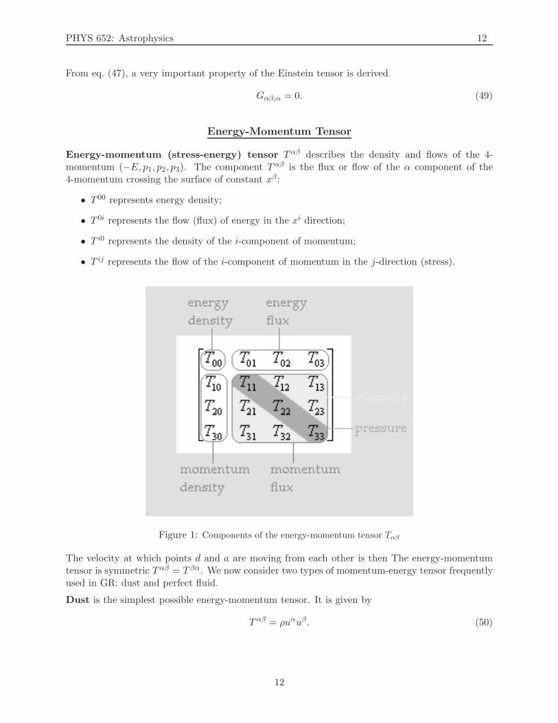
Energy-momentum (stress-energy) tensor Tαβ describes the density and flows of the 4-momentum (−E, p1, p2, p3). The component Tαβ is the flux or flow of the α component of the4-momentum crossing the surface of constant xβ:
• T 00 represents energy density;
• T 0i represents the flow (flux) of energy in the xi direction;
• T i0 represents the density of the i-component of momentum;
• T ij represents the flow of the i-component of momentum in the j-direction (stress).
Figure 1: Components of the energy-momentum tensor Tαβ
The velocity at which points d and a are moving from each other is then The energy-momentumtensor is symmetric Tαβ = T βα. We now consider two types of momentum-energy tensor frequentlyused in GR: dust and perfect fluid.
Dust is the simplest possible energy-momentum tensor. It is given by
Tαβ = ρuαuβ. (50)
12
PHYS 652: Astrophysics 13
For a comoving observer, the 4-velocity is given by ~u = (1, 0, 0, 0), so the stress-energy tensorreduces to
Tαβ =
ρ 0 0 00 0 0 00 0 0 00 0 0 0
. (51)
Dust is an approximation of the Universe at later times, when radiation is negligible.
Perfect fluid is a fluid that has no heat conduction or viscosity. It is fully parametrized by itsmass density ρ and the pressure P . It is given by
Tαβ = (ρ+ P )uαuβ + Pgαβ . (52)
For a comoving observer, the 4-velocity is given by ~u = (1, 0, 0, 0), so the stress-energy tensorreduces to
Tαβ =
ρ 0 0 00 P 0 00 0 P 00 0 0 P
. (53)
In the limit of P → 0, the perfect fluid approximation reduces to that of dust. Perfect fluid is anapproximation of the Universe at earlier times, when radiation dominates.Conservation equations for the energy-momentum tensor Tαβ are simply given by
Tαβ;β = 0. (54)
This expression incorporates both energy and momentum conservations in a general metric. In thelimit of flat spacetime (Minkowski metric), it reduces to
∂Tαβ
∂xβ= 0, (55)
from which the traditional expressions for the conservation of momentum and energy are readilyrecovered.
Evolution of Energy
Conservation of energy given in eq. (54) can be used to determine how components of theenergy-momentum tensor evolve with time. Following the notation in the textbook, the mixedenergy-momentum tensor is:
Tαβ =
−ρ 0 0 00 P 0 00 0 P 00 0 0 P
. (56)
and its conservation is given by
T µν;µ ≡ ∂T µν
∂xµ+ ΓµαµT
αν = ΓανµT
µα , (57)
which gives four separate equations. Consider ν = 0 component:
∂T µ0∂xµ
+ ΓµαµTα0 − Γα0µT
µα = 0. (58)
13
PHYS 652: Astrophysics 14
Because of isotropy, all non-diagonal terms of Tαβ vanish, so T i0 = 0. This leads to µ = 0 in thefirst term and α = 0 in the second term above. Thus
∂T 00
∂x0+ Γµ0µT
00 − Γα0µT
µα = 0,
−∂ρ
∂t− Γµ0µρ− Γα0µT
µα = 0. (59)
Expanding flat spacetime is described by the flat Friedmann-Lemaıtre-Robertson-Walker metrictensor given in eq. (10):
gαβ =
−1 0 0 00 a2(t) 0 00 0 a2(t) 00 0 0 a2(t)
. (60)
From the definition of the Christoffel symbol
Γανµ ≡ 1
2gαγ (gνγ,µ + gγµ,ν − gνβ,γ) (61)
Γα0µ =1
2gαγ (g0γ,µ + gγµ,0 − g0β,γ)
=1
2gαγgγµ,0 because g0γ = const., g0β = const.,
=
12
(
δαγa−2)
(2δγµaa) if α 6= 0 and µ 6= 0,0 if α = 0 or µ = 0,
because gγ0,0 = 0, g0µ,0 = 0,
so that the only non-zero Γα0µ is Γi0i = a/a (note: when summed over repeated indices Γi0i = 3a/a).So, the conservation law in the expanding Universe from eq. (59) becomes
∂ρ
∂t+ 3
a
aρ+
a
aTαα = 0
∂ρ
∂t+ 3 (ρ+ P )
a
a= 0. (62)
We can massage this to get
a−3∂[
ρa3]
∂t= −3
a
aP, (63)
and use it to find out how both matter and radiation scale with expansion. For matter (dustapproximation), we have zero pressure Pm = 0, so
∂[
ρma3]
∂t= −3a2aPm = 0, (64)
which means that the energy density of matter scales as ρm ∝ a−3. This should come as nosurprise, because the total amount of matter Mm is conserved, and the volume of the Universe goesas V ∝ a3, so ρm ∝ Mm
V ∝ a−3.For radiation, Pr = ρr/3, so from eq. (62) we obtain
∂ρr∂t
− a
a4ρr = a−4
[
∂ρra4]
∂t= 0,
which implies that ρr ∝ a−4. This too should not surprise us — since radiation density is directlyproportional to the energy per particle and inversely proportional to the total volume, i.e., ρr ∝nr~νV ∝ nr~
λV ∝ a−4, because λ ∝ a. The last part states that the energy per particle decreases asthe Universe expands.
14
PHYS 652: Astrophysics 15
Einstein’s Field Equations
The stage is now set for deriving and understanding Einstein’s field equations.The GR must present appropriate analogues of the two parts of the dynamical picture: 1) how
particles move in response to gravity; and 2) how particles generate gravitational effects. The firstpart was answered when we derived the geodesic equation as the analogue of the Newton’s SecondLaw. The second part requires finding the analogue of the Poisson equation
∇2Φ(~x) = 4πGρ(~x), (65)
which specifies how matter curves spacetime. It should also be obvious by now that all equations inGR must be in tensor form. Arguably the most enlightening derivation of the Einstein’s equationsis to argue about its form on physical grounds, which was the approach originally adopted byEinstein.
In Newtonian gravity, the rest mass generates gravitational effects. From SR, however, welearned that the rest mass is just one form of energy, and that the mass and energy are equivalent.Therefore, we should expect that in GR all sources of both energy and momentum contribute togenerating spacetime curvature. This means that in GR, the energy-momentum tensor Tαβ is thesource for spacetime curvature in the same sense that the mass density ρ is the source for thepotential Φ. So, at this point, we can say that we have a pretty good idea of what the RHS of theGR analogue of the Poisson equation should be: κTαβ (where κ is some constant to be determinedlater).
What about the LHS of the GR analogue of the Poisson equation? What is analogous to∇2Φ(~x)? As we have seen earlier (eq. (39)), the spacetime metric in the Newtonian limit is modifiedby a term proportional to Φ. If we extend this analogy, then the GR counterpart of ~∇Φ in the RHSof the Newton’s Second Law should include derivatives of the metric, which is indeed verified by theform of the geodesic equation (see eqs. (14), (31)). Further extending this analogy, one would expectthat, the GR counterpart of ∇2Φ(~x) would contain terms which contain second derivatives of themetric. From eq. (41), we see that the Riemann tensor Rαβγδ — and consequently its contractionsRicci tensor Rαβ and Ricci scalar R — contain second derivatives of the metric, and thus becomeviable candidates for the LHS of the Einstein’s field equation.
Lead by this line of reasoning, Einstein originally suggested that the field equation might read
Rαβ = κTαβ , (66)
but it was quickly recognized that this cannot be correct, because while the conservation of energy-momentum require Tαβ;α = 0, the same is in general not true of the Ricci tensor: Rαβ
;α 6= 0. Fortu-nately, Einstein’s tensor Gαβ (a combination of Ricci tensor and Ricci scalar), satisfies the require-ment that it has vanishing divergence. Therefore, Einstein’s equation then becomes
Gαβ ≡ Rαβ −1
2gαβR = κTαβ , (67)
By matching Einstein’s equation in the Newtonian limit to the Poisson equation, the constant κ isfound to be 8πG/c4, so Einstein’s field equations become (after obeying our notation c = 1):
Rαβ −1
2gαβR = 8πGTαβ. (68)
15
PHYS 652: Astrophysics 16
4 Lecture 4: The Cosmological Metric
“The most exciting phrase to hear in science, the one that heralds new discoveries, is not ‘Eureka!’but ‘That’s funny...’ ”
Isaac Asimov
The Big Picture: Last time we derived Einstein’s equations — a GR analog to Poisson equation— which describe how matter and radiation curve ambient spacetime. Today, we are going toderive the Friedmann-Lemaıtre-Robertson-Walker metrics for both flat and curved spacetimes inspherical coordinates, and look at the particular solutions for Universes with different contents.
The “standard model” of the Universe is founded on the Cosmological Principle which statesthat our Universe is — at all times — homogeneous (same from point to point) and isotropic(same view in all directions) when viewed on the large scales (galaxies, galaxy clusters, galaxysuper-clusters, etc. are considered as “local inhomogeneities”).
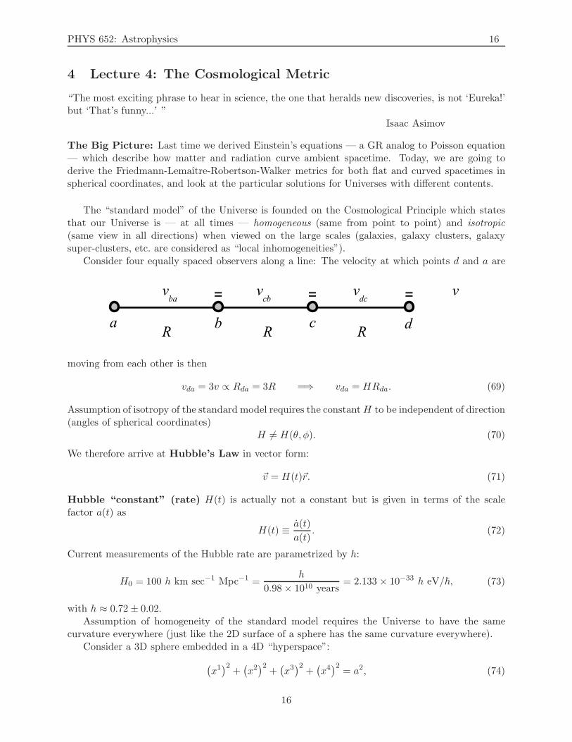
Consider four equally spaced observers along a line: The velocity at which points d and a are
moving from each other is then
vda = 3v ∝ Rda = 3R =⇒ vda = HRda. (69)
Assumption of isotropy of the standard model requires the constantH to be independent of direction(angles of spherical coordinates)
H 6= H(θ, φ). (70)
We therefore arrive at Hubble’s Law in vector form:
~v = H(t)~r. (71)
Hubble “constant” (rate) H(t) is actually not a constant but is given in terms of the scalefactor a(t) as
H(t) ≡ a(t)
a(t). (72)
Current measurements of the Hubble rate are parametrized by h:
H0 = 100 h km sec−1 Mpc−1 =h
0.98× 10¹⁰ years= 2.133 × 10⁻³³ h eV/~, (73)
with h ≈ 0.72± 0.02.Assumption of homogeneity of the standard model requires the Universe to have the same
curvature everywhere (just like the 2D surface of a sphere has the same curvature everywhere).Consider a 3D sphere embedded in a 4D “hyperspace”:
(
x1)2
+(
x2)2
+(
x3)2
+(
x4)2
= a2, (74)
16
PHYS 652: Astrophysics 17
where a is the radius of the 3D sphere. The distance between two points in 4D space is given by
dl2 =(
dx1)2
+(
dx2)2
+(
dx3)2
+(
dx4)2
, (75)
Differentiating eq. (74) and solving for dx4, we obtain
dx4 = − xidxi√a2 − xixi
, recall i = 1, 2, 3 (76)
so that eq. (75) now reads
dl2 =(
dx1)2
+(
dx2)2
+(
dx3)2
+
(
xidxi)2
a2 − xixi. (77)
In spherical coordinates
x1 = r sin θ cosφ,
x2 = r sin θ sinφ,
x3 = r cos θ,
so
dxidxi = dr2 + r2dθ2 + (r sin θ)2 dφ2,
xidxi = rdr,
xixi = r2.
Finally, we obtain
dl2 =r2dr2
a2 − r2+ dr2 + r2dθ2 + (r sin θ)2 dφ2,
dl2 =dr2
1−(
ra
)2 + r2dθ2 + (r sin θ)2 dφ2. (78)
We could also have a negatively curved object (a “saddle”) with a2 ≡ −a2, or a flat (zero curvature,Euclidian) space with a → ∞. In literature, the short-hand notation is adopted:
dl2 =dr2
1− k(
ra
)2 + r2dθ2 + (r sin θ)2 dφ2, (79)
ds2 = −dt2 +dr2
1− k(
ra
)2 + r2dθ2 + (r sin θ)2 dφ2, (80)
k =
+1 positive-curvature Universe (finite, closed),0 flat Universe (infinite, open),
−1 negative-curvature Universe (infinite, open).(81)
To isolate time-dependent term a, make the following substitution:
r =
a sinχ positive-curvature Universe,aχ flat Universe,a sinhχ negative-curvature Universe.
17
PHYS 652: Astrophysics 18
Thendl2 = a2
[
dχ2 +Σ2(χ)(
dθ2 + sin2 θdφ2)]
. (82)
where
Σ(χ) ≡
sinχ positive-curvature Universe,χ flat Universe,sinhχ negative-curvature Universe.
(Important note: for small χ, sinχ ≈ χ, sinhχ ≈ χ. What does it mean?)If we introduce the “arc-parameter measure of time” (“conformal time”)
dη ≡ dt
a(t), (83)
then we can express the 4D line element in terms of Friedman-Lemaıtre-Robertson-Walker metric:
ds2 = a2(η)[
−dη2 + dχ2 +Σ2(χ)(
dθ2 + sin2 θdφ2)]
. (84)
Friedmann Equations
We can now solve Einstein’s field equations for the perfect fluid. All the calculations are donein a comoving frame where
u0 = 1 = −u0, and ui = ui = 0. (85)
This means that the energy-momentum tensor is given by
Tαβ = (ρ+ P )uαuβ + Pgαβ . (86)
Raising an index of the Einstein’s field equation
Rαβ −1
2gαβR = 8πGTαβ, (87)
we obtain
Rαβ − 1
2δαβR = 8πGTαβ . (88)
(Recall gαβgβν = δαν ). After contracting over indices α and β, we obtain
−R = 8πGT, where T ≡ Tαα , (89)
which means that Einstein’s field equation can be rewritten as
Rαβ = 8πG
(
Tαβ − 1
2δαβT
)
. (90)
For the perfect fluid, it is easily found that
T = − (ρ+ P ) + 4P = −ρ+ 3P, (91)
so the eq. (90) becomes
Rαβ = 8πG
[
(ρ+ P )uαuβ +1
2(ρ− P )δαβ .
]
. (92)
18
PHYS 652: Astrophysics 19
After straightforward yet tedious calculations (which I relegate to homework), we obtain the com-ponents of the Ricci tensor:
R00 = 3
a
a,
R0i = 0,
Rij =
1
a2(
aa+ 2a2 + 2k)
δαβ .
(93)
The t− t component of the Einstein’s equation given in eq. (92) becomes
3a
a= 8πG
[
−(ρ+ P ) +1
2(ρ− P )
]
, (94)
or
a = −4πG
3(ρ+ 3P ) a. (95)
The i− i component of the Einstein’s equation is
1
a2(
aa+ 2a2 + 2k)
= 8πG
[
1
2(ρ− P )
]
, (96)
oraa+ 2a2 + 2k = 4πG(ρ− P )a2, (97)
The eqs. (95)-(97) are the basic equations connecting the scale factor a to ρ and P . To obtain aclosed system of equations, we only need an equation of state P = P (ρ), which relates P and ρ.The system then reduces to two equations for two unknowns a and ρ.
It is, however, beneficial to further massage these basic equations into a set that is more easilysolved. Solving the eq. (97) for a, we obtain
a = 4πG(ρ− P )a− 2a2
a+
2k
a, (98)
which can be combined with eq. (95) to cancel out P dependence and yield
16πGρa
3− 2k
a− 2a2
a= 0, (99)
or
a2 + k =8πG
3ρa2. (100)
When combined with the eq. (62) derived in the context of conservation of energy-momentumtensor, and the equation of state, we obtain a closed system of Friedmann equations:
a2 + k =8πG
3ρa2, (101a)
∂ρ
∂t+ 3 (ρ+ P )
a
a= 0, (101b)
P = P (ρ). (101c)
19
PHYS 652: Astrophysics 20
5 Lecture 5: Solutions of Friedmann Equations
“A man gazing at the stars is proverbially at the mercy of the puddles in the road.”Alexander Smith
The Big Picture: Last time we derived Friedmann equations — a closed set of solutions ofEinstein’s equations which relate the scale factor a(t), energy density ρ and the pressure P for flat,open and closed Universe (as denoted by curvature constant k = 0, 1,−1). Today we are going tosolve Friedmann equations for the matter-dominated and radiation-dominated Universe and obtainthe form of the scale factor a(t). We will also estimate the age of the flat Friedmann Universe.
From the definition of the Hubble rate H in eq. (72)
H ≡ a
a=⇒ (102)
H = −H2 +a
a= −H2
(
1− a
H2a
)
≡ −H2 (1 + q) , (103)
we define a deceleration parameter q as
q ≡ − a
H2a. (104)
Non-relativistic matter-dominated Universe is modeled by dust approximation: P = 0.Then, from eq. (95), we have
a
a+
4πG
3ρ = 0, (105)
and, in terms of H
−H2q +4πG
3ρ = 0. (106)
Therefore
ρ =3H2
4πGq. (107)
Then the first Friedmann equation becomes
(
a
a
)2
− 8πG
3ρ = − k
a2,
H2 − 2H2q = − k
a2, (108)
so−k = a2H2(1− 2q). (109)
Since both a 6= 0 and H 6= 0, for flat Universe (k = 0), q = 1/2 (q > 1/2 for k = 1 and q < 1/2 fork = −1). When combined with eq. (107), this yields critical density
ρcr =3H2
8πG, (110)
20
PHYS 652: Astrophysics 21
the density needed to yield the flat Universe. Currently, it is (see eq. (73))
ρcr =3H2
0
8πG=
3(
h0.98×1010 years
)2 (1 year
3600×24×365 sec
)2
8π (6.67 × 10⁻⁸cm3 g−1 s−2)= 1.87× 10⁻²⁹h2
g
cm3≈ 10−29 g
cm3.
(We used h ≈ 0.72 ± 0.02.)It is important to note that the quantity q provides the relationship between the density of the
Universe ρ and the critical density ρcr (after combining eqs. (107) and (109)):
q =ρ
2ρcr. (111)
The second Friedmann equation (eq. (101b)) for the matter-dominated Universe becomes
ρ+ 3ρa
a= 0
a3ρ+ 3ρaa2 = 0 ⇒ d
dt
(
a3ρ)
= 0 ⇒ a3ρ = a30ρ0 = const. (112)
Radiation-dominated Universe is modeled by perfect fluid approximation with P = 13ρ.
The second Friedmann equation (eq. (101b)) becomes
ρ+ 3
(
ρ+1
3ρ
)
a
a= ρ+ 4ρ
a
a= 0
a4ρ+ 4ρaa3 = 0 ⇒ d
dt
(
a4ρ)
= 0 ⇒ a4ρ = a40ρ0 = const. (113)
Flat Universe (k = 0, q0 =12)
Matter-dominated (dust approximation): P = 0, a3ρ = const.The first Friedmann equation (eq. (101a)) becomes
a2
a2=
8πG
3ρ0
(a0a
)3
⇒ da
dt=
√
8πGρ0a30
3
1
a1/2⇒
∫
a1/2da =2
3a3/2 +K =
√
8πGρ0a30
3t. (114)
At the Big Bang, t = 0, a = 0, so K = 0. Upon adopting convention a0 = 1, and the factthat the Universe is flat ρ0 = ρcr, we finally have
a = (6πGρ0)1/3 t2/3 = (6πGρcr)
1/3 t2/3
=
(
6πG3H2
0
8πG
)1/3
t2/3 =
(
9H20
4
)1/3
t2/3 =
(
3H0
2
)2/3
t2/3. (115)
where we have used the eq. (110) in the second step. From here we compute the age of theUniverse t0, which corresponds to the Hubble rate H0 and the scale factor a = a0 = 1 to be:
t0 =2
3H0. (116)
Taking H0 =h
0.98×10¹⁰ yearsand h ≈ 72, we get
t0 =2× 0.98× 1010 years
3× 0.72≈ 9.1 × 10⁹ years ≡ 9.1 A (aeon). (117)
21
PHYS 652: Astrophysics 22
Radiation-dominated: P = 13ρ, a4ρ = const.
The first Friedmann equation (eq. (101a)) becomes
a2
a2=
8πG
3ρ0
(a0a
)4
⇒ da
dt=
√
8πGρ0a403
1
a⇒
∫
ada =1
2a2 +K =
√
8πGρ0a403
t. (118)
Again, at the Big Bang, t = 0, a = 0, so K = 0, and a0=1. Also ρ0 = ρcr. Therefore,
a =
(
32
3πGρ0
)1/4
t1/2 =
(
32
3πGρcr
)1/4
t1/2 =
(
32
3πG
3H20
8πG
)1/4
t1/2 = (2H0)1/2 t1/2. (119)
a(t)
t
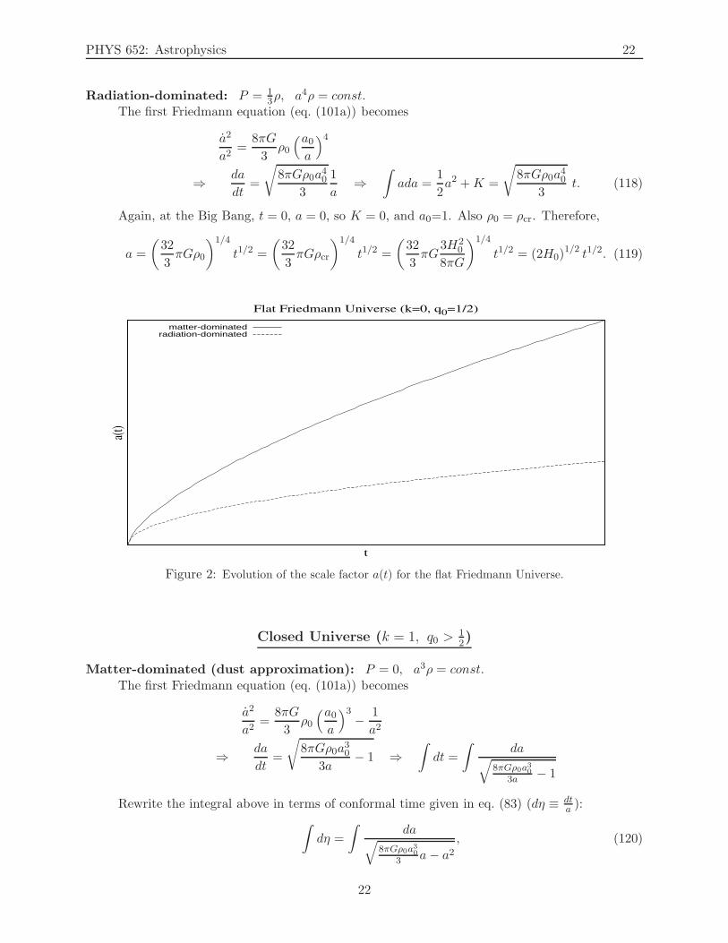
Flat Friedmann Universe (k=0, q0=1/2)
matter-dominatedradiation-dominated
Figure 2: Evolution of the scale factor a(t) for the flat Friedmann Universe.
Closed Universe (k = 1, q0 >12)
Matter-dominated (dust approximation): P = 0, a3ρ = const.The first Friedmann equation (eq. (101a)) becomes
a2
a2=
8πG
3ρ0
(a0a
)3− 1
a2
⇒ da
dt=
√
8πGρ0a30
3a− 1 ⇒
∫
dt =
∫
da√
8πGρ0a303a − 1
Rewrite the integral above in terms of conformal time given in eq. (83) (dη ≡ dta ):
∫
dη =
∫
da√
8πGρ0a303 a− a2
, (120)
22
PHYS 652: Astrophysics 23
and define, after substituting a0 = 1 and using eqs. (107)-(109)
A ≡ 4πGρ03
= H20q0 =
q02q0 − 1
. (121)
Then
η − η0 =
∫ a
0
da√2Aa− a2
= sin−1
(
a−A
A
)
+1
2π. (122)
But, the requirement η = 0 at a = 0 sets η0 = 0, so we have
a−A
A= sin
(
η − 1
2π
)
= − cos η ⇒ a = A(1− cos η). (123)
Now dt = adη, so
t− t0 =
∫
adη =
∫
A(1 − cos η)dη = A
∫
(1− cos η) dη = A(η − sin η). (124)
But, the requirement η = 0 at t = 0 sets t0 = 0. Therefore, we finally have the dependenceof the scale factor a in terms of the time t parametrized by the conformal time η as:
a =q0
2q0 − 1(1− cos η), (125)
t =q0
2q0 − 1(η − sin η).
Radiation-dominated: P = 13ρ, a4ρ = const.
The first Friedmann equation (eq. (101a)) becomes
a2
a2=
8πG
3ρ0
(a0a
)4− 1
a2
⇒ da
dt=
√
8πGρ0a40
3a2− 1 ⇒
∫
dt =
∫
da√
8πGρ0a303a2
− 1
Again, rewrite the integral above in terms of conformal time and quantity A1 =8πGρ0
3 = 2q02q0−1 :
η − η0 =
∫ a
0
da√A1 − a2
= sin−1
(
a√A1
)
. (126)
Again, the requirement η = 0 at a = 0 sets η0 = 0, so we have
a =√
A1 sin (η) , (127)
andt− t0 =
√
A1 cos (η) , (128)
The requirement η = 0 at t = 0 sets t0 =√A1, so we finally have
a =
√
2q02q0 − 1
sin η, (129)
t =
√
2q02q0 − 1
(1− cos η) .
23
PHYS 652: Astrophysics 24
a(t)
t
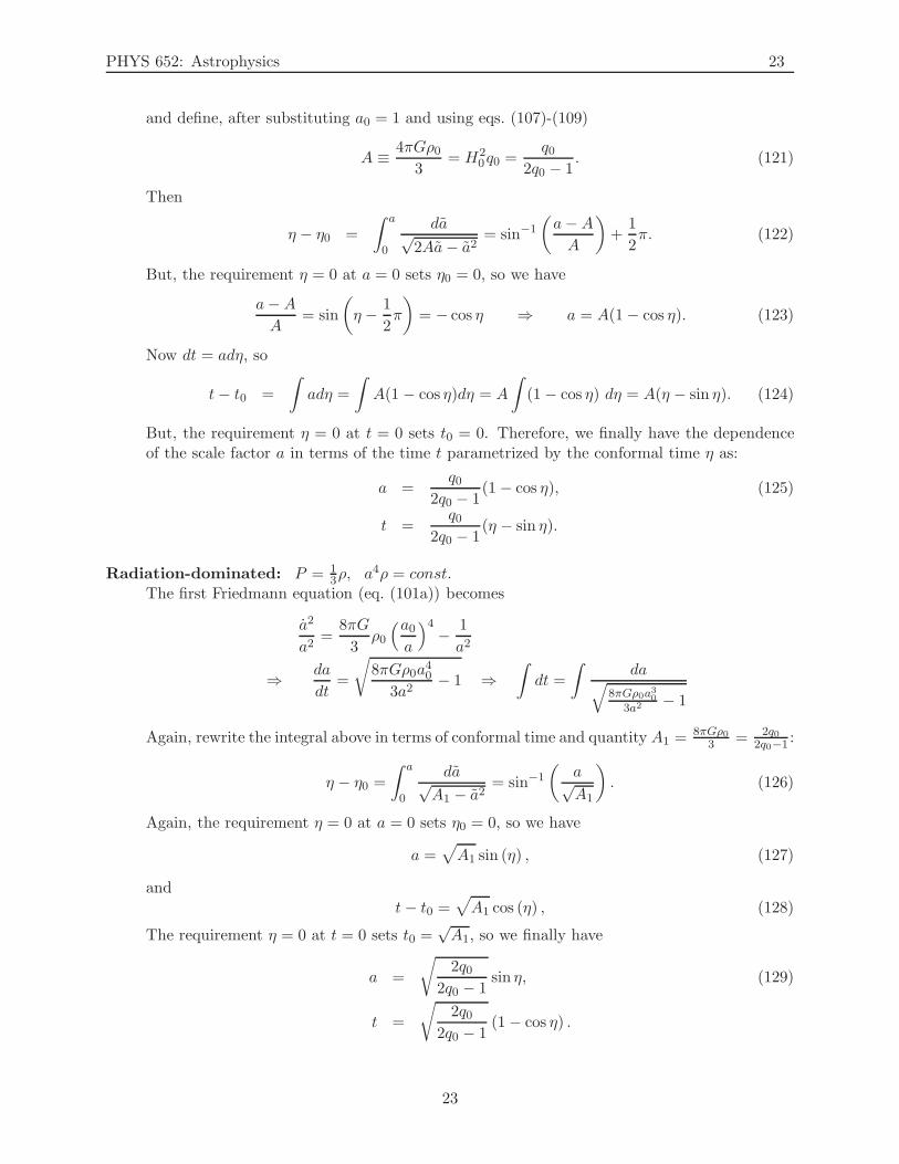
Closed Friedmann Universe (k=1, q0>1/2)
Big CrunchBig Crunch
matter-dominatedradiation-dominated
Figure 3: Evolution of the scale factor a(t) for the closed Friedmann Universe.
In both matter- and radiation-dominated closed Universes, the evolution is cycloidal — the scalefactor grows at an ever-decreasing rate until it reaches a point at which the expansion is halted andreversed. The Universe then starts to compress and it finally collapses in the Big Crunch.
Open Universe (k = −1, q0 <12)
Matter-dominated (dust approximation): P = 0, a3ρ = const.The first Friedmann equation (eq. (101a)) becomes
a2
a2=
8πG
3ρ0
(a0a
)3+
1
a2
⇒ da
dt=
√
8πGρ0a30
3a+ 1 ⇒
∫
dt =
∫
da√
8πGρ0a303a + 1
Again, rewrite the integral above in terms of conformal time:∫
dη =
∫
da√
8πGρ0a303 a+ a2
, (130)
take a0 = 1, and define A ≡ 4πGρ03 = q0
2q0−1 . Then
η − η0 =
∫ a
0
da√
2Aa+ a2= ln
a+ A+√
a(2A+ a)
A
= ln
a
A+ 1 +
√
2a
A+
(
a
A
)2
= cosh−1
(
a
A+ 1
)
. (131)
But, the requirement η = 0 at a = 0 sets η0 = 0, so we have
a+ A
A= cosh η ⇒ a = A(cosh η − 1). (132)
24
PHYS 652: Astrophysics 25
Now dt = adη, so
t− t0 =
∫
adη =
∫
A(cosh η − 1)dη = A
∫
(cosh η − 1) dη = A(sinh η − η). (133)
But, the requirement η = 0 at t = 0 sets t0 = 0. Therefore, we finally have the dependenceof the scale factor a in terms of the time t parametrized by the conformal time η as:
a =q0
2q0 − 1(cosh η − 1), (134)
t =q0
2q0 − 1(sinh η − η).
Radiation-dominated: P = 13ρ, a4ρ = const.
The first Friedmann equation (eq. (101a)) becomes
a2
a2=
8πG
3ρ0
(a0a
)4+
1
a2
⇒ da
dt=
√
8πGρ0a403a2
+ 1 ⇒∫
dt =
∫
da√
8πGρ0a303a2
+ 1
Again, rewrite the integral above in terms of conformal time and quantity A1 ≡ 8πGρ03 = 2q0
2q0−1 :
η − η0 =
∫ a
0
da√
A1 + a2= sinh−1
(
a√
A1
)
(135)
Again, the requirement η = 0 at a = 0 sets η0 = 0, so we have
a =
√
A1 sinh η, (136)
t− t0 =
√
A1 cosh η, (137)
The requirement η = 0 at t = 0 sets t0 =√
A1, so we finally have
a =
√
2q01− 2q0
sinh η, (138)
t =
√
2q01− 2q0
(cosh η − 1) .
Early times (small η limit): For small values of η, the trigonometric and hyperbolic functionscan be expanded in Taylor series (keeping only first two terms):
sin η = η − 1
6η3, cos η = 1− 1
2η2,
sinh η = η +1
6η3, cosh η = 1 +
1
2η2,
so, to the leading term, the a and t dependence on η for the different curvatures is shown in thetable below:
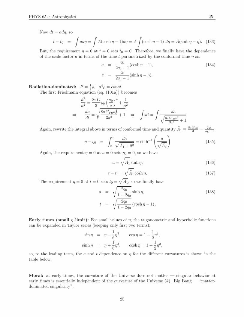
Moral: at early times, the curvature of the Universe does not matter — singular behavior atearly times is essentially independent of the curvature of the Universe (k). Big Bang — “matter-dominated singularity”.
25
PHYS 652: Astrophysics 26
a(t)
t
Open Friedmann Universe (k=-1, q0<1/2)
matter-dominatedradiation-dominated
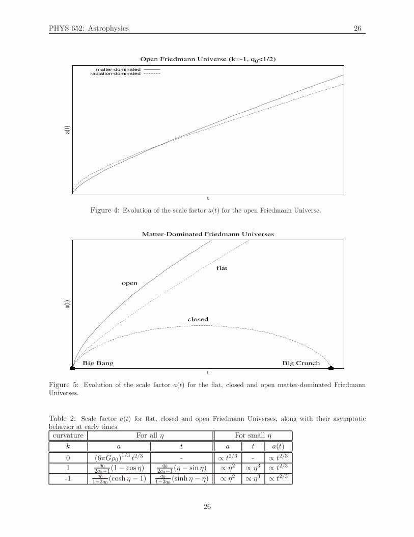
Figure 4: Evolution of the scale factor a(t) for the open Friedmann Universe.
a(t)
t
Matter-Dominated Friedmann Universes
closed
open
flat
Big CrunchBig Bang
Figure 5: Evolution of the scale factor a(t) for the flat, closed and open matter-dominated FriedmannUniverses.
Table 2: Scale factor a(t) for flat, closed and open Friedmann Universes, along with their asymptoticbehavior at early times.
curvature For all η For small η
k a t a t a(t)
0 (6πGρ0)1/3 t2/3 - ∝ t2/3 - ∝ t2/3
1 q02q0−1(1− cos η) q0
2q0−1(η − sin η) ∝ η2 ∝ η3 ∝ t2/3
-1 q01−2q0
(cosh η − 1) q01−2q0
(sinh η − η) ∝ η2 ∝ η3 ∝ t2/3
26
PHYS 652: Astrophysics 27
6 Lecture 6: Age of the Universe
“The effort to understand the Universe is one of the very few things that lifts human life a littleabove the level of farce, and gives it some of the grace of tragedy.”
Steven Weinberg
The Big Picture: Last time we solved Friedmann equations for the matter-dominated andradiation-dominated flat, open and closed Universes and obtained the form of the scale factora(t). We computed the critical density needed to have a flat Universe at about 10−29 gcm−3. Wealso estimated the age of the flat Friedmann Universe to about 9 billion years. Today we are goingto combine the information discovered by observations of CMB radiation with the solutions of theFriedmann equations to present strong evidence for an additional vacuum energy and non-baryonicmatter — dark energy and dark matter.
Age of a Matter-Dominated Friedmann Universe
At the present time, t = t0 (age of the Universe), a(t0) = a0 = 1 and q = q0, so the eq. (107)provides the link between the total current density of the Universe and the critical density:
q0 =ρ02ρcr
. (139)
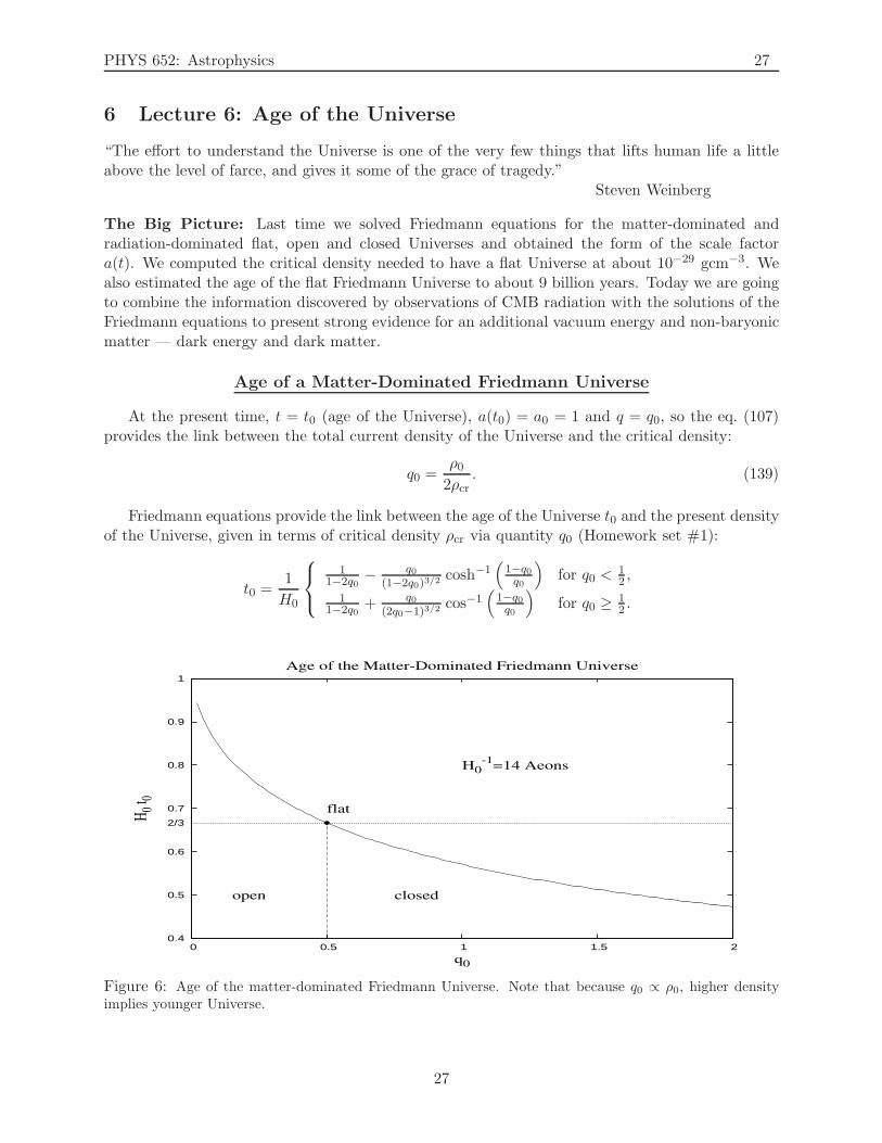
Friedmann equations provide the link between the age of the Universe t0 and the present densityof the Universe, given in terms of critical density ρcr via quantity q0 (Homework set #1):
t0 =1
H0
11−2q0
− q0(1−2q0)3/2
cosh−1(
1−q0q0
)
for q0 <12 ,
11−2q0
+ q0(2q0−1)3/2
cos−1(
1−q0q0
)
for q0 ≥ 12 .
0.4
0.5
0.6
0.7
0.8
0.9
1
0 0.5 1 1.5 2
H0 t 0
q0
Age of the Matter-Dominated Friedmann Universe
flat
open closed
H0-1
=14 Aeons
2/3
Figure 6: Age of the matter-dominated Friedmann Universe. Note that because q0 ∝ ρ0, higher densityimplies younger Universe.
27
PHYS 652: Astrophysics 28
However, the observations, such as Wilkinson Microwave Anisotropy Probe (WMAP) finds theage of the Universe to be
t0 = 13.7 ± 0.2A, (140)
which would — from the graph above — imply that q0 ≈ 0, that is ρ0 ≈ 0 — there is no matterin the Universe! But that is not the case — WMAP data also indicates that the Universe is (very)nearly flat, so q0 = 1/2. Hmmm... Something is wrong with the matter-dominated FriedmannUniverse — it is missing most of its energy density.
Einstein’s Field Equations Revisited: Cosmological Constant
Einstein first introduced the cosmological constant Λ in his field equations in order to getaround at the time embarrassing solution — non-steady-state Universe. Einstein’s equations withthe cosmological constant had a form
Rαβ −1
2gαβR+ gαβΛ = 8πGTαβ. (141)
or, alternatively
Rαβ − 1
2R+ Λ = 8πGTαβ , (142)
Rαβ − 1
2R = 8πGTαβ , (143)
where Tαβ = Tαβ − Λ and
Tαβ =
−ρ− Λ8πG 0 0 0
0 P − Λ8πG 0 0
0 0 P − Λ8πG 0
0 0 0 P − Λ8πG
. (144)
The new energy-momentum tensor Tαβ reveals the nature of the cosmological constant Λ — it is asource of energy density and the inverse pressure (opposing the pressure of matter). Indeed, thisis what led to the coining of the name dark energy.
The density of dark energy does not depend on the scale factor a. The conservation law (andalso the second Friedmann equation) (eq. 62)
∂ρ
∂t+ 3 (ρ+ P )
a
a= 0. (145)
then implies that the equation of state for the dark energy is P (ρ) = −ρ. More generally, since theequations of state for the matter is P (ρ) = 0 and radiation P (ρ) = 1
3ρ, they can all be expressed as
P (ρ) = wρ, (146)
where the parameter w = −1 for dark energy w = 0 for matter and w = 1/3 for radiation.Consider a mixture of matter and dark energy:
ρ = ρm + ρde = ρm0
(a0a
)3+ ρde. (147)
28
PHYS 652: Astrophysics 29
Define
Ωm0 ≡ 8πG
3H20
ρm0 =ρm0
ρcr0,
Ωde0 ≡ 8πG
3H20
ρde0 =ρde0ρcr0
. (148)
Now rewrite the first Friedmann equation (eq. (101a)):
(
a
a
)2
− 8πG
3ρ = − k
a2(
a
a
)2
−H20Ωm0
(a0a
)3−H2
0Ωde0 = − k
a2(149)
Combining eqs. (109) and (111), we have
−k = a2H2(1− ΩT), (150)
where
ΩT ≡ 2q =ρ
ρcr= Ωm +Ωde. (151)
From WMAP observations the Universe is nearly flat, so k = 0, which leads to
ΩT = ΩT0 = Ωm0 +Ωde0 = 1, (152)
⇒ Ωm0 = 1− Ωde0, (153)
and, after taking a0 = 1(
a
a
)2
= H20
[
(1− Ωde0)1
a3+Ωde0
]
. (154)
Solving for a, this becomes
a = H0
√
1− Ωde0
a+Ωde0a2, (155)
and
H0t0 =
∫ 1
0
da√
1−Ωde0a +Ωde0a2
=
∫ 1
0
a1/2da√
(1− Ωde0) + Ωde0a3
=2
3√Ωde0
ln[
2(
√
Ωde0a3 +√
Ωde0(a3 − 1) + 1)]
∣
∣
∣
∣
1
0
=2
3√Ωde0
ln
(
1 +√Ωde0√
1− Ωde0
)
, (156)
so the age of the Universe with dark energy is
t0 =2
3H0
√Ωde0
ln
(
1 +√Ωde0√
1− Ωde0
)
. (157)
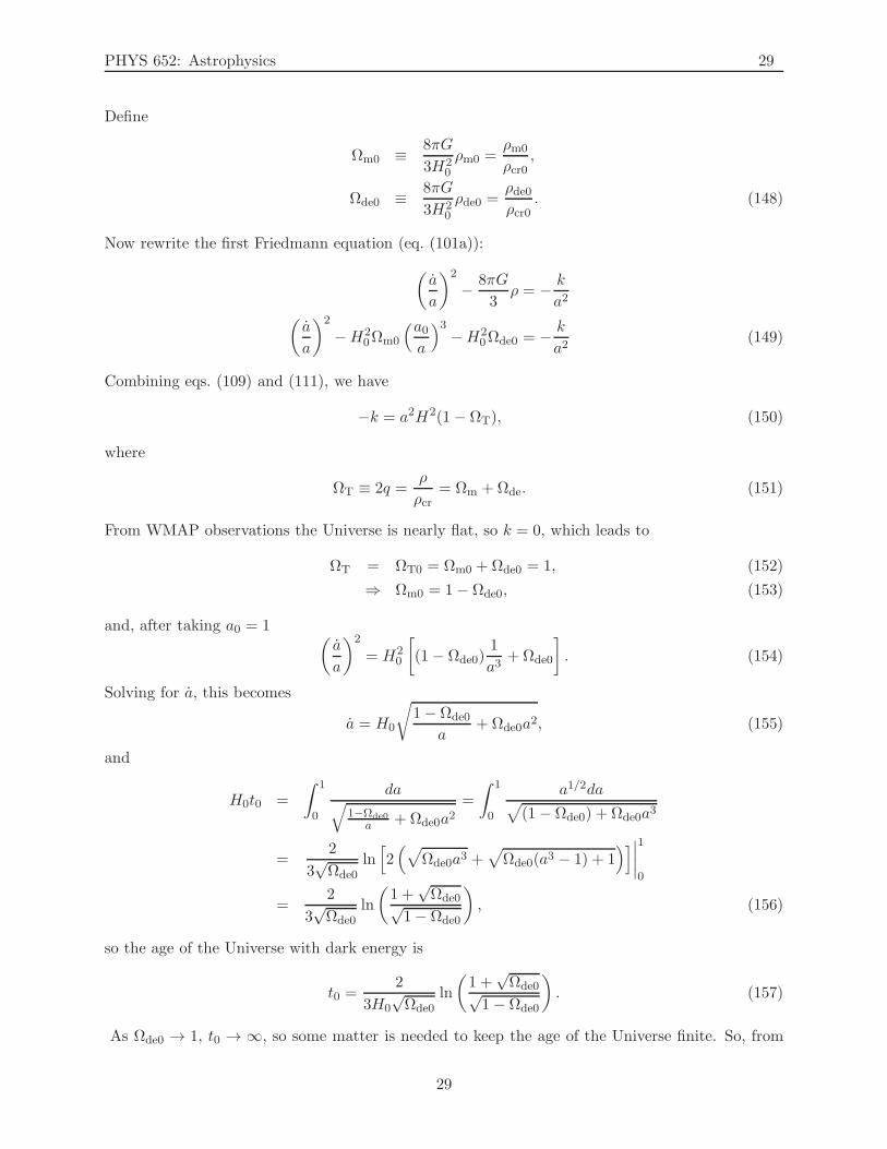
As Ωde0 → 1, t0 → ∞, so some matter is needed to keep the age of the Universe finite. So, from
29
PHYS 652: Astrophysics 30
10
11
12
13
14
15
0 0.1 0.2 0.3 0.4 0.5 0.6 0.7 0.8
t 0 [Aeo
ns]
Ωde0
Age of the Universe with a Cosmological Constant
13.7
Ωde0=0.72
t0=13.7 Aeons
Figure 7: Age of the Universe with a cosmological constant Λ. The age of the Universe of 13.7A correspondsto Ωde0 ≈ 0.72.
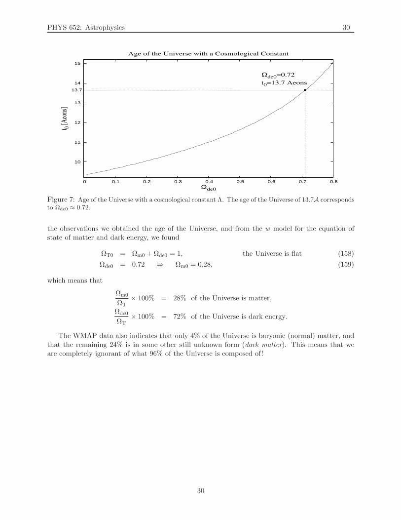
the observations we obtained the age of the Universe, and from the w model for the equation ofstate of matter and dark energy, we found
ΩT0 = Ωm0 +Ωde0 = 1, the Universe is flat (158)
Ωde0 = 0.72 ⇒ Ωm0 = 0.28, (159)
which means that
Ωm0
ΩT× 100% = 28% of the Universe is matter,
Ωde0
ΩT× 100% = 72% of the Universe is dark energy.
The WMAP data also indicates that only 4% of the Universe is baryonic (normal) matter, andthat the remaining 24% is in some other still unknown form (dark matter). This means that weare completely ignorant of what 96% of the Universe is composed of!
30
PHYS 652: Astrophysics 31
-4
-2
0
2
4
6
8
10
12
14
1e-04 0.001 0.01 0.1 1
log 10
[ρ(t)/
ρ cr]
a(t)
Energy Density Vs. Scale Factor
matterradiation
dark energy (Λ)
today
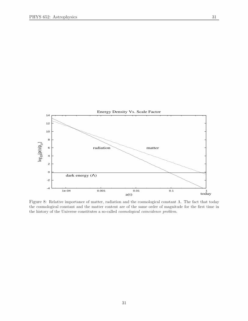
Figure 8: Relative importance of matter, radiation and the cosmological constant Λ. The fact that todaythe cosmological constant and the matter content are of the same order of magnitude for the first time inthe history of the Universe constitutes a so-called cosmological coincidence problem.
31
PHYS 652: Astrophysics 32
7 Lecture 7: Cosmic Distances
“Science never solves a problem without creating ten more.”George Bernard Shaw
The Big Picture: Last time we introduced the dark energy as the dominant driving mechanism forthe cosmic expansion. Today we are going to introduce the redshift as a consequence of expansionof the Universe, and introduce the relevant lengths associated with an expanding Universe.
Redshift
If the wavelength of the emission line in the laboratory is λ0 and if the observed wavelength isλ > λ0, then the line is said to be redshifted by a fraction z (the redshift) given by
z =λ− λ0
λ0. (160)
The redshift is a natural consequence of the Doppler effect — as the Universe expands at a rate a,the wavelength of a particle scales as
λ =λ0
a, (161)
which, combined with eq. (160) yields
z =1− a
a, (162)
a =1
1 + z. (163)
Gravitational redshift is observed when a receiver is located at a higher gravitational potentialthan the source. The physical explanation is that the particle loses a fraction of the energy (andhence increases its wavelength) by overcoming the difference in the potential (climbing out of thepotential well).
Comoving Coordinates
GR states that the laws of physics are the same in any coordinates. However, some coordinatesare easier to work with then others. One such set of coordinates are comoving coordinates inwhich an observer is comoving with the Hubble flow. Only for these observers in the comovingcoordinates, the Universe is isotropic (otherwise, portions of the Universe will exhibit a systematicbias: portions of the sky will appear systematically blue- or red-shifted).
Comoving Horizon
Comoving horizon is defined as the total portion of the Universe visible to the observer. Itrepresents the sphere with radius equal to the distance the light could have traveled (in the absenceof interactions) since the Big Bang (t = 0). In time dt, light travels a comoving distance dη =dx/a = cdt/a, where dx is a physical distance. After recalling convention adopted earlier c = 1,becomes
η ≡∫ t
0
dt′
a(t′). (164)
32
PHYS 652: Astrophysics 33
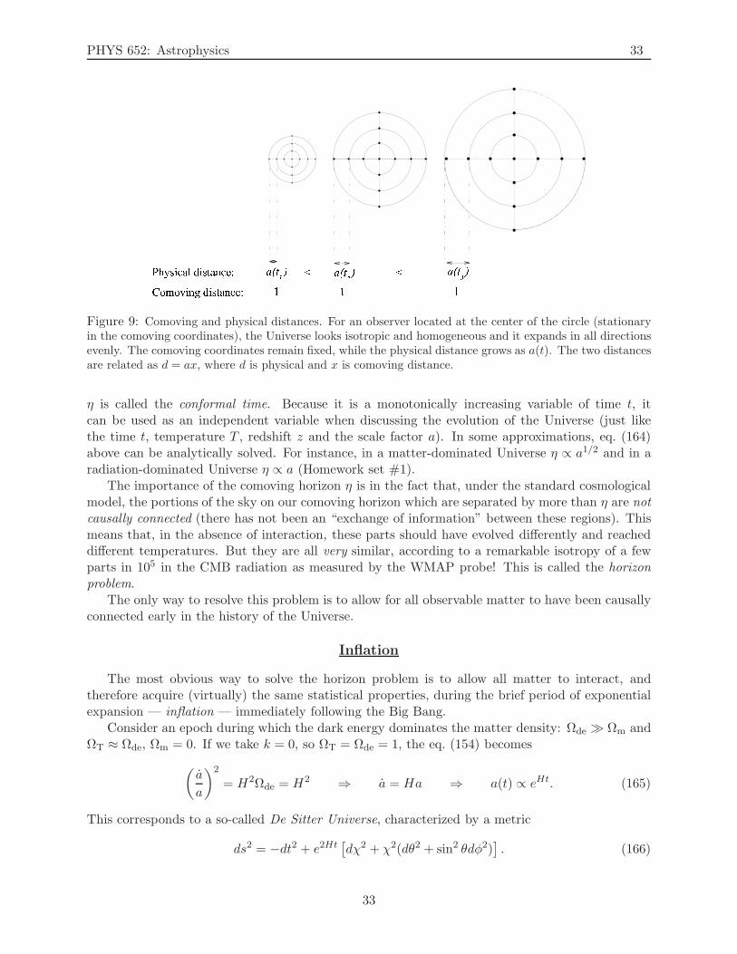
Figure 9: Comoving and physical distances. For an observer located at the center of the circle (stationaryin the comoving coordinates), the Universe looks isotropic and homogeneous and it expands in all directionsevenly. The comoving coordinates remain fixed, while the physical distance grows as a(t). The two distancesare related as d = ax, where d is physical and x is comoving distance.
η is called the conformal time. Because it is a monotonically increasing variable of time t, itcan be used as an independent variable when discussing the evolution of the Universe (just likethe time t, temperature T , redshift z and the scale factor a). In some approximations, eq. (164)above can be analytically solved. For instance, in a matter-dominated Universe η ∝ a1/2 and in aradiation-dominated Universe η ∝ a (Homework set #1).
The importance of the comoving horizon η is in the fact that, under the standard cosmologicalmodel, the portions of the sky on our comoving horizon which are separated by more than η are notcausally connected (there has not been an “exchange of information” between these regions). Thismeans that, in the absence of interaction, these parts should have evolved differently and reacheddifferent temperatures. But they are all very similar, according to a remarkable isotropy of a fewparts in 105 in the CMB radiation as measured by the WMAP probe! This is called the horizonproblem.
The only way to resolve this problem is to allow for all observable matter to have been causallyconnected early in the history of the Universe.
Inflation
The most obvious way to solve the horizon problem is to allow all matter to interact, andtherefore acquire (virtually) the same statistical properties, during the brief period of exponentialexpansion — inflation — immediately following the Big Bang.
Consider an epoch during which the dark energy dominates the matter density: Ωde ≫ Ωm andΩT ≈ Ωde, Ωm = 0. If we take k = 0, so ΩT = Ωde = 1, the eq. (154) becomes
(
a
a
)2
= H2Ωde = H2 ⇒ a = Ha ⇒ a(t) ∝ eHt. (165)
This corresponds to a so-called De Sitter Universe, characterized by a metric
ds2 = −dt2 + e2Ht[
dχ2 + χ2(dθ2 + sin2 θdφ2)]
. (166)
33
PHYS 652: Astrophysics 34
We are heading toward de Sitter Universe, because the density of dark energy remains constant,while the matter density scales as a−3 and radiation density as a−4, which makes the dark energyan ever-increasing part of the cosmic inventory.
The exponential expansion of the scale factor (see eq. (165)) means that the physical distancebetween any two observers will eventually be growing faster than the speed of light. At that pointthose two observers will, of course, not be able to have any contact anymore. Eventually, we willnot be able to observe any galaxies other than the Milky Way and a handful of others in thegravitationally-bound Local Group cluster of galaxies.
If we consider that the expansion occurred about the time that the strong force “froze out” (att = tGUT ), then
H ≈ 1
tGUT≈ 1
10−36 s= 1036 s−1, (167)
which is an extremely fast e-folding time, indicating staggering rate of inflation. In just a fewe-folding times, the Universe is already huge.
From eq. (150), we have
(1− ΩT) = − k
a2H2, (168)
which means that ΩT → 1 very fast, regardless of the value of k (recall, we noted earlier that thecurvature is relatively unimportant early in the history of the Universe — the behavior of flat,closed and open Universes are asymptotically identical as t → 0). It also means that after inflationΩT = 1 — the Universe is flat.
We are heading toward de Sitter Universe, because the density of dark energy remains constant,while the energy density of matter drops off as a3 (see Fig. (8)).
Inflation solves the flatness problem: The WMAP showed that the Universe is flat (or at leastvery nearly flat), i.e., ΩT ≈ 1. Why is this so? Why 1? Why not, say, 10−5 or 106? The standardmodel does not provide an reasonable explanation for the flat Universe. The problem is exasperatedsince the ΩT = 1, and thus the flat Universe, is the unstable fixed point. This means that if theUniverse started with ΩT = 1 exactly, it would remain so forever. If, however, the Universe wascreated with any other value of ΩT, even one arbitrarily close, the separation between the value ofΩT and 1 would grow over time, presuming only that the scale factor a grows slower then linearlyin time. Let us demonstrate this mathematically.
The first Friedmann equation (eq. (101a))
a2 + k =8πG
3ρa2, (169)
can be rewritten to yield
ρ =3
8πGa2(
a2 + k)
. (170)
Dividing by the critical mass
ρcr =3H2
8πG, (171)
yields
ΩT =ρ
ρcr=⇒ ΩT − 1 =
ρ− ρcrρcr
=3k
8πGa28πGa2
3a2=
k
a2. (172)
It is easily seen that if for t → 0 a → ∞ then ΩT − 1 → 0.
34
PHYS 652: Astrophysics 35
If a = a0
(
tt0
)p, then
a = a0t−p0 ptp−1, (173)
so thatk
a2=
k
a20p2t2p0 p2t2(1−p) ≡ kt2(1−p). (174)
Finally, we obtainΩT − 1 = kt2(1−p), (175)
so that ΩT − 1 → 0 as t → 0 for p < 1.
ΩT − 1 → 0 as t → 0 for p < 1,
ΩT − 1 → ∞ as t → ∞ for p < 1. (176)
This means that the magnitude of ΩT−1 grows with increasing t. In other words, during the entirehistory of the Universe over which the scale factor a scales sub-linearly, the Universe is growingincreasingly non-flat (unless ΩT is exactly equal to unity). In the language of mathematics, ΩT = 1is an unstable fixed point for p < 1.
Equation (175) holds a clue as to how to naturally obtain a flat Universe, in accordance toobservations: change the dynamics so that ΩT = 1 is a stable fixed point. All that is required isthat the scale factor grows super-linearly (for example p > 1 in the equations above). If one allowsfor a cosmological constant, so that a grows exponentially in time with a(t) = exp[Ht] (eq. (165)),then
a = HeHt, (177)
so that
ΩT − 1 =ρ− ρcrρcr
=3k
8πGa28πGa2
3a2=
k
a2=
k
H2e−2Ht. (178)
It follows that any initial deviation from unity is squashed exponentially. If, at some early timein its history, the Universe underwent a period of exponential expansion (inflation), any initialdeviation from ΩT = 1 would be reduced to the point extremely close to unity, so much so thateven the prolonged subsequent evolution with a ∝ tp with p < 1, would not drive it appreciablyaway from it. Therefore, inflation solves the flatness problem.
Distance to an Emitter
It is often useful to determine the distance between a distant emitter and us. In comovingcoordinates, the distance to an object at a scale factor a (or alternatively redshift z = 1/a− 1) is
χ ≡∫ t(0)
t(a)
dt′
a(t′)=
∫ 1
a
da′
a′2H(a′), (179)
after the change of variables da/dt = aH. For the portion of the Universe which we can observe,which is to about z ≤ 6, the radiation which dominated early on can be ignored. For the purelymatter-dominated flat Universe, we can combine the definition of the Hubble rate H ≡ a/a andeq. (115) to obtain
H =a
a=
2(
3H02
)2/3t−1/3
3(
3H02
)2/3t2/3
=2
3t=
2
3 23H0
a3/2= H0a
−3/2. (180)
35
PHYS 652: Astrophysics 36
This simplifies the integral in eq. (179) to
χf,MD(a) =1
H0
∫ 1
a
da′
a′1/2χ =
2
H0a′
1/2
∣
∣
∣
∣
1
a
=2
H0
[
1− a1/2]
, (181)
where superscripts f and MD denote flat and matter-dominated Universe. In terms of the redshiftz eq. (181) becomes (after recalling z = 1/a− 1):
χf,MD(z) =2
H0
[
1− 1√1 + z
]
. (182)
For small redshift z, 1/√1 + z ≈ 1− z/2, so χf (z) ≈ z/H0. For large redshift z, χ(z) → 2/H0.
Angular Diameter Distance
Another important distance in astronomy is the angular diameter distance. In astronomy, theangular diameter distance is determined by measuring the angle θ subtended by an object of knownphysical size l. Assuming that the angle is small, it is given by
dA =l
θ. (183)
To compute the angular diameter distance in an expanding Universe, we express the quantities land θ in comoving coordinates. The comoving size of an object of physical size l is simply l/a,while the angle subtended in the flat Friedmann Universe is
θ =la
χ(a), (184)
so finally we have
df,MDA = aχ =
χ
1 + z. (185)
For small redshift z, df,MDA ≈ χ. At large z, df,MD
A → χ/z → 2/(zH0), so the angular diameterdistance decreases with redshift z. This means that the in the flat Universe, objects at largeredshifts appear larger than they would at intermediate redshifts!
Luminosity Distance
In astronomy, distances can be inferred by measuring the flux from an object of known lumi-nosity (“standard candles”). Flux and luminosity are related through
F ≡ L
4πd2, (186)
since the total luminosity through a spherical constant with area 4πd2 is constant. The totalluminosity is defined as the amount of energy radiated per unit time. This means L ≡ dE
dt . Assumingthat, without loss of generality, all the N photons radiated have the same frequency ν (wavelengthλ). Then the luminosity becomes L = ~
λdNdt . In comoving coordinates λc = λ/a and the t-derivative
is replaced by η-derivative (recall dt = adη), so
L(χ) =~
λc
dN
dη= a
~
λ
dN
dta =
~
λ
dN
dta2 = La2. (187)
36
PHYS 652: Astrophysics 37
Then the observed flux is
F =La2
4πχ2=
L
4π(χa
)2 ≡ L
4πd2L, (188)
wheredL ≡ χ
a, (189)
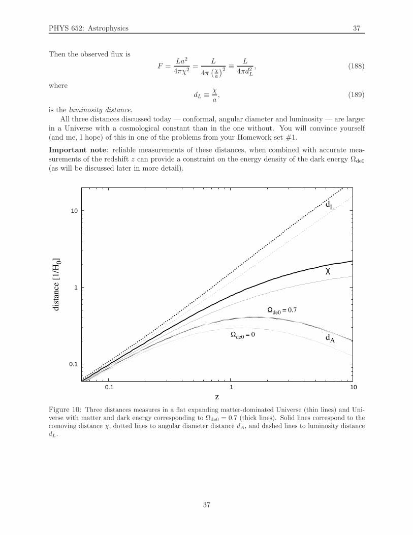
is the luminosity distance.All three distances discussed today — conformal, angular diameter and luminosity — are larger
in a Universe with a cosmological constant than in the one without. You will convince yourself(and me, I hope) of this in one of the problems from your Homework set #1.
Important note: reliable measurements of these distances, when combined with accurate mea-surements of the redshift z can provide a constraint on the energy density of the dark energy Ωde0
(as will be discussed later in more detail).
0.1
1
10
0.1 1 10
dis
tance
[1/H
0]
z
dL
χ
dAΩde0 = 0
Ωde0 = 0.7
Figure 10: Three distances measures in a flat expanding matter-dominated Universe (thin lines) and Uni-verse with matter and dark energy corresponding to Ωde0 = 0.7 (thick lines). Solid lines correspond to thecomoving distance χ, dotted lines to angular diameter distance dA, and dashed lines to luminosity distancedL.
37
PHYS 652: Astrophysics 38
8 Lecture 8: Summary of Foundations of Cosmology
“Shall I refuse my dinner because I do not fully understand the process of digestion?”Oliver Heaviside
The Big Picture: In the past seven lectures, we introduced and reviewed the basic ideas of GR asthey pertain to the understanding of the Universe on the largest scales. We derived the equationsof GR which describe the dynamics in a curved spacetime — geodesic equation and the Einstein’sequations. Solving Einstein’s equations, both with and without the cosmological constant, leads todifferent cosmologies, which depend on both curvature — flat, closed and open — and content ofthe Universe — matter, radiation and dark (vacuum) energy. Today we review these concepts.
General Relativity: Dynamics in Curved Spacetime
GR describes the dynamics in curved spacetime through two equations:
• Geodesic equation: how a particle moves in curved spacetime (GR analogy to Newton’s SecondLaw in flat Euclidian space).
xν = −Γνγδxγxδ. (190)
• Einstein’s equations: how mass and energy distort (curve) spacetime (GR analogy to Poissonequation which describes how mass distribution creates a force field in Newtonian mechanics).
Rαβ − 1
2R+ Λ = 8πGTαβ , (191)
where Λ is a cosmological constant corresponding to “vacuum” energy (dark energy).Solving Einstein’s equations in FLRW metric
ds2 = −dt2 + a2[
dχ2 +Σ2(χ)(
dθ2 + sin2 θdφ2)]
. (192)
with (possibly) evolving space (through the scale factor a(t), which does not have to be time-dependent a priori, leads to Friedmann’s equations:
a2 + k =8πG
3ρa2, (193a)
ρ+ 3 (ρ+ P )a
a= 0, (193b)
P = P (ρ). (193c)
We have looked at two different equations of state P = P (ρ):
• Dust approximation for matter-dominated Universe: in comoving coordinates, the matter isapproximated as stationary dust particles which produce no pressure — P = 0.
• Perfect fluid approximation for radiation-dominated Universe: the pressure induced by themovement of relativistic particles is P = 1
3ρ.
• Vacuum (dark) energy for dark energy-dominated Universe: P = −ρ.
More generally, we expressed these equations of state through a w parameter, defined as
w ≡ P
ρ. (194)
38
PHYS 652: Astrophysics 39
Table 3: Parameter w for the equations of state in different regimes.
regime w scaling with a(t)
radiation-dominated 1/3 ∝ a−4
matter-dominated 0 ∝ a−3
dark energy-dominated −1 ∝ 1
Cosmology: Solutions to Friedmann’s Equations
To specify a cosmology, we use Friedmann’s equations and choose:
1. Curvature of the Universe:
• flat: k = 0,
• closed: k = +1,
• open: k = −1;
2. Equation of state (dominating regime given in Table 3).
Expanding Universe
Solving the Friedmann’s equation yields a number of different cosmologies, which we derivedand discussed in class. Some of these predict age of the Universe which is grossly wrong, leading usto believe that the underlying assumptions were incorrect. The observations show that the Universeis very nearly flat, so we focus on the flat k = 0 cosmology. Solving for the scale factor a(t) inthe flat Universe — without any additional a priori assumptions — we obtain that the Universeis expanding, and that its expansion is decelerating during the radiation- and matter-dominatedepochs, and accelerating during the dark energy-dominated epoch (see Table 4). Observations alsoshow us what the current relative content of the Universe is — how much of the critical density isfound in radiation (about 0.005%), baryonic (about 4%) and dark matter (about 24%) and darkenergy (about 72%). Using how these different constituents scale with the scale factor a(t) (seeTable 3), we can compute when each of the constituents dominated (Fig. 12).
Table 4: Scale factor a(t) for different regimes in the flat Universe.
regime a(t) a(t) a(t)
radiation-dominated ∝ t1/2 ∝ t−1/2 > 0 expanding ∝ −t3/2 < 0 decelerating
matter-dominated ∝ t2/3 ∝ t−1/3 > 0 expanding ∝ −t4/3 < 0 decelerating
dark energy-dominated ∝ eHt ∝ eHt > 0 expanding ∝ eHt > 0 accelerating
39
PHYS 652: Astrophysics 40
10
1
10-1
10-2
10-3
10-4
10-5
10-6
10210110-110-210-310-410-510-610-710-810-9
a(t)
t [Aeons]
aeq
aeq2
radiation-dominated
matter-dominated
Λ-dom.
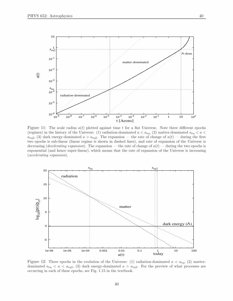
Figure 11: The scale radius a(t) plotted against time t for a flat Universe. Note three different epochs(regimes) in the history of the Universe: (1) radiation-dominated a < aeq, (2) matter-dominated aeq < a <aeq2, (3) dark energy-dominated a > aeq2. The expansion — the rate of change of a(t) — during the firsttwo epochs is sub-linear (linear regime is shown in dashed lines), and rate of expansion of the Universe isdecreasing (decelerating expansion). The expansion — the rate of change of a(t) — during the two epochs isexponential (and hence super-linear), which means that the rate of expansion of the Universe is increasing(accelerating expansion).
-5
0
5
10
15
20
1e-06 1e-05 1e-04 0.001 0.01 0.1 1 10 100
log 10
[ρ(t
)/ρ cr
]
a(t)
matter
radiation
dark energy (Λ)
today
aeq aeq2
Figure 12: Three epochs in the evolution of the Universe: (1) radiation-dominated a < aeq, (2) matter-dominated aeq < a < aeq2, (3) dark energy-dominated a > aeq2. For the preview of what processes areoccurring in each of these epochs, see Fig. 1.15 in the textbook.
40
PHYS 652: Astrophysics 41
9 Lecture 9: Cosmic Inventory I: Radiation
“Happy is he who gets to know the reasons for things.”Virgil (70 – 19 BC; Roman poet)
The Big Picture: Last time we talked about inflation early in Universe’s history as the currently-prevailing explanation for the horizon problem and the observed flatness of the Universe. Todaywe are going to talk about the radiation contents of the Universe: photons and neutrinos, andtheir relative abundances. Next time, we’ll complete this with matter content: baryonic and darkmatter. Later yet, we will talk about the dark energy.
Distribution Function of Species
The distribution function of different species is given by Bose-Einstein distribution for bosons(particles with an integer spin, such as photons, W and Z bosons, gluons, gravitons, mesons, etc.):
fBE =1
e(E−µ)/T − 1, (195)
and Fermi-Dirac distribution for fermions (particles with a half-integer spin, such as quarks,baryons, leptons, etc.):
fFD =1
e(E−µ)/T + 1, (196)
where E(p) =√
p2 +m2 and µ is the chemical potential, which is much smaller than the temper-ature T for almost all particles at almost all times, and can therefore be safely ignored in mostof the calculations. These distributions are for the smooth Universe, and represent a zero-orderapproximation. They, therefore, do not depend on positions ~x or on the direction of the momentum~p, but only on the magnitude of the momentum p.
The properties of species specified by the distribution function f(~x, ~p) are computed by inte-grating quantities over the distribution function. For example, the energy density of a specie i, ρiis given by
ρi = gi
∫
d3p
(2π)3fi(~x, ~p)E(p), (197)
where gi is the degeneracy of the species (for instance, gi = 2 for the photon for its spin states).The factor 1/(2π~)3 is the consequence of Heisenberg’s uncertainty principle, which states that noparticle can be localized in a phase-space volume smaller than (2π~)3, so this becomes the unit sizeof the phase-space.
Similarly, the pressure of a specie i can be expressed as
Pi = gi
∫
d3p
(2π)3fi(~x, ~p)
p2
3E(p). (198)
Entropy Density
Entropy density is defined as (when chemical potential is negligible, as is the case in almost allcases in cosmology):
s ≡ ρ+ P
T. (199)
41
PHYS 652: Astrophysics 42
To compute how the entropy density scales with the scale factor a, rewrite the second Friedmannequation (eq. (101b)):
ρ+ 3 (ρ+ P )a
a= 0
a−3 ∂[
ρa3]
∂t+ 3
a
aP = 0
a−3∂[
(ρ+ P )a3]
∂t− ∂P
∂t= 0,
Combining the equation above with the the result (Homework set #1)
∂P
∂T=
ρ+ P
T, (200)
and the fact that, due to chain rule,∂P
∂t=
∂P
∂T
∂T
∂t, (201)
we obtain
a−3∂[
(ρ+ P )a3]
∂t− ∂T
∂t
ρ+ P
T= a−3T
∂
∂t
[
(ρ+ P )a3
T
]
= 0. (202)
The quantity in brackets is constant, so
(ρ+ P )a3
T= sa3 = const., (203)
and entropy density scales as a−3. This results holds for total entropy density for a mixture ofspecies in equilibrium, even if two species have different temperatures. The importance of thisresult will be obvious soon when we use it to compute the relative temperatures of neutrinos andphotons in the Universe.
Photons
The energy density due to CMB radiation can be found by using eq. (197) with the Bose-Einsteindistribution given in eq. (195):
ργ = gγ
∫
d3p
(2π)3E(p)
eE/Tγ − 1= 2
∫
d3p
(2π)3p
ep/Tγ − 1, (204)
where we have used gγ = 2, E(p) =√
p2 +m2 = p for massless photons, and neglected the chemicalpotential µ. After noting that d3p = 4πp2dp, and making a substitution x = p/Tγ
ργ =8π
(2π)3
∫ ∞
0
p3
ep/Tγ − 1dp =
8π
(2π)3T 4γ
∫ ∞
0
x3
ex − 1dx
=8π
(2π)3T 4γ 6ζ(4) =
8π
(2π)3T 4γ
π4
15
⇒ ργ =π2
15T 4γ , (205)
where we have used the result∫ ∞
0
x3
ex − 1dx = 6ζ(4) =
π4
15. (206)
42
PHYS 652: Astrophysics 43
We have derived earlier that the energy density of radiation scales as ργ ∝ a−4 (see eq. (65)). Since,from eq. (205), ργ ∝ T 4
γ , we see that Tγ ∝ a−1. This means
Tγa = Tγ0a0 = Tγ0
⇒ Tγ =Tγ0a
=2.725K
a, (207)
where Tγ0 = 2.725K is the temperature of the CMB measured today (we also used a0 = 1).In terms of the critical density ρcr, we have
Ωγ ≡ ργρcr
=π2
15T 4γ
1
ρcr=
π2
15
(
2.725K
a
)4 1
8.098 × 10⁻¹¹h2eV4 , (208)
where the value for ρcr is found from the Appendix B, page 416 in the textbook. We now use therelationship between Kelvin and eV: 11605 K = 1 eV, so the above equation becomes
Ωγ =ργρcr
=π2
15
(
2.725K
a
)4 1
8.098 × 10⁻¹¹h2 (11605K)4=
2.47× 10⁻⁵
h2a4. (209)
If we take h ≈ 0.72, then the fractional content of the Universe due to CMB radiation today is
Ωγ |today = Ωγ0 ≡ργ0ρcr0
= 4.76 × 10⁻⁵. (210)
Neutrinos
Cosmic neutrinos have not been directly observed, because they are weakly interacting particles.Neutrinos are leptons, and hence fermions, so they are subject to Fermi-Dirac distribution.
In order to compute the relative energy density of neutrinos, we need to relate the temperatureof neutrinos to the temperature of photons in CMB radiation.
Neutrinos were once in equilibrium with the rest of the cosmic plasma. They decoupled fromthe hot plasma before the annihilation of electrons and positrons when the cosmic temperaturereached roughly the electron mass. We therefore invoke an argument based on entropy density,which we have shown to decay as a−3 (eq. (203)).
Before the annihilation (and before the decoupling of neutrinos), the plasma has a uniformtemperature of, say, T1 (also let a = a1). The pressure due to CMB radiation (photons) is given by
Pγ =1
3ργ , (211)
so the contribution to the entropy for each spin state is (recall eq. (205) has a factor gγ = 2 reflecting2 spin states)
sγ =ργ + Pγ
T1=
4
3T1ργ =
4
3T1
1
2
π2
15T 41 = 2
π2
45T 31 . (212)
Photons are bosons, and hence subject to Bose-Einstein statistics, which, as we saw in eq. (206)leads to the integral
IBE ≡∫ ∞
0
x3
ex − 1dx = 6ζ(4) =
π4
15. (213)
Computation of the energy density for fermions will lead to the integration over the Fermi-Diracdistribution function, which will lead to the integral
IFD ≡∫ ∞
0
x3
ex + 1dx =
7
48ζ(4) =
7π4
120=
7
8IBE . (214)
43
PHYS 652: Astrophysics 44
Therefore, the contribution of massless fermions will be 7/8 of the contribution of massless bosons.Before the annihilation, there are the following fermions: electrons (2 spin states), positrons (2spin states), neutrinos (3 generations and 1 spin state) and anti-neutrinos (3 generations and 1 spinstate), and the following bosons: photons (2 spin states). Therefore, before the annihilation, theentropy density is given by the sum of all entropies of species:
s(a1) = 2π2
45T 31
[
2 +7
8(2 + 2 + 3 + 3)
]
=43π2
90T 31 . (215)
After annihilation, temperatures of photons and neutrinos are no longer equal. Neutrinosdecoupled slightly before the annihilation, after which their temperature Tν scales as a−1 (justlike for photons). Photons were still coupled to the plasma during the annihilation, which raisedtheir temperature Tγ . The electrons and positrons are annihilated – converted into high-energyphotons which quickly reach equilibrium with the other photons, effectively raising their equilibriumtemperature Tγ . The entropy density after the annihilation (at some a = a2) is therefore
s(a2) = 2π2
45
[
2T 3γ +
7
86T 3
ν
]
= 4π2
45
[
T 3γ +
21
8T 3ν
]
. (216)
But, entropy density s scales as a−3, so
sa3 = s(a1)a31 = s(a2)a
32, (217)
which leads to43π2
90T 31 a
31 = 4
π2
45
[
T 3γ +
21
8T 3ν
]
a32. (218)
Neutrino temperature scales throughout as a−1:
Ta = T1a1 = Tνa2, (219)
so
43π2
90T 31 a
31 =
43π2
90(T1a1)
3 =43π2
90(Tνa2)
3 = 4π2
45
[
(
TγTν
)3
+21
8
]
(Tνa2)3,
⇒ 43
8=
(
TγTν
)3
+21
8⇒(
TγTν
)3
=22
8
⇒ TγTν
=
(
11
4
)1/3
≈ 1.4, orTνTγ
=
(
4
11
)1/3
≈ 0.71. (220)
This means that the neutrino temperature is lower by about a factor (4/11)1/3 (about 29%) thenthe CMB radiation (photon) temperature, which was heated by the annihilation of electrons andpositrons.
Now that we can relate the temperature of neutrinos Tν to the temperature of photons Tγ(which we measure to be today to be 2.725K), we can compute the energy density of the neutrinos(which are fermions, and hence subject to Fermi-Dirac distribution function):
ρν = gν
∫
d3p
(2π)3E(p)
eE/Tν + 1= 6
∫
d3p
(2π)3p
ep/Tν + 1, (221)
44
PHYS 652: Astrophysics 45
where gν = 6 (6 flavors — νe, νµ, ντ , νe, νµ, ντ ), E(p) =√
p2 +m2 = p for massless neutrinos, andneglected the chemical potential µ. After noting that d3p = 4πp2dp, and making a substitutionx = p/Tν
ρν =24π
(2π)3
∫ ∞
0
p3
ep/Tν + 1dp =
24π
(2π)3T 4ν
∫ ∞
0
x3
ex + 1dx
=24π
(2π)3T 4ν IFD =
3π
π3T 4ν
7
8
π4
15
⇒ ρν =7π2
40T 4ν =
7π2
40
(
4
11
)4/3
T 4γ , (222)
or in terms of energy density of photons
ρν =7
4015
(
4
11
)4/3 π2
15T 4γ
⇒ ρν =21
8
(
4
11
)4/3
ργ . (223)
We also have
Ων =21
8
(
4
11
)4/3
Ωγ =21
8
(
4
11
)4/3 2.47 × 10⁻⁵
h2a4=
1.65 × 10⁻⁵
h2a4, (224)
so that the ratio of the neutrino density to the critical density today is
Ων |today ≡ Ων0 =1.65 × 10⁻⁵
h2. (225)
All of the calculations above were done assuming that the neutrinos are massless. However, obser-vations of solar neutrinos indicate that they change flavors on their way from Sun to us, which canonly happen if they have mass. The observations of atmospheric neutrinos suggest that at least oneneutrino has mass larger than 0.05eV. In that case, for a massive neutrino, E(p) =
√
p2 +m2ν 6= p,
so the integral in eq. (222) becomes (with gν = 2 for one flavor of neutrinos with 2 spin states)
ρν =8π
(2π)3
∫ ∞
0
p2√
p2 +m2ν
e√p2+m2
ν/Tν + 1dp. (226)
45
PHYS 652: Astrophysics 46
10 Lecture 10: Cosmic Inventory II: Baryonic and Dark Matter
“The least deviation from the truth is multiplied later.”Aristotle
The Big Picture: Last time we talked about the radiation contents of the Universe: photons andneutrinos and their relative abundances. Today we are going to talk about the dark matter — itshistorical background, evidence for it and its importance.
Baryonic Matter
When using the term “baryonic matter”, both baryons and electrons are implied. Electrons arenot baryons, but leptons, but given that the mass of an electron is nearly 2000 times smaller thanthe mass of a proton or a neutron, electron contribution is negligible.
Unlike the energy density of CMB radiation, which can be described as a gas with a temperatureand vanishing chemical potential, the baryonic density must be directly measured. The differentmethods which measure baryonic density at varying redshifts z largely agree to be about 2 − 5%of the critical density today:
Ωb|today ≡ Ωb0 ≡ρb0ρcr0
= 0.02 − 0.05. (227)
We also know that the total amount of baryonic matter is constant, so with the expanding Universe,the fractional energy density scales as ρb ∝ a−3, so
Ωb =ρbρcr0
=ρb0ρcr0
a−3 = Ωb0a−3. (228)
Several methods are used to gauge the baryon content of the Universe:
1. Directly observing visible matter in galaxies. It has been found that the largest contributioncomes from the gas in galaxy clusters, while stars in galaxies account for only a comparativelysmall fraction. This approach estimates Ωb0 = 0.02.
2. Looking at spectra of distant galaxies, and measuring the amount of light absorption. Theamount of light absorbed quantifies the amount of hydrogen the light encounters along theway. Baryon density is then inferred from the estimate of the amount of hydrogen. Thisapproach roughly estimates Ωb0h
1.5 ≈ 0.02 (Rauch et al. 1997, Astrophysical Journal, 489,7).
3. Computing the baryon content of the Universe from the anisotropies of the CMB radiation.This approach puts fairly stringent limits on the baryon content to about Ωb0h
2 = 0.024+0.004−0.003.
4. Inferring the baryon content of the Universe form the light element abundances. These pindown the baryon content to Ωb0h
2 = 0.0205 ± 0.0018.
These estimates are in fairly good agreement. They put a rough baryonic content of the Universeat about 2 − 5% of the critical density. However, as we shall soon see, the total matter density inthe Universe is significantly higher than that, so there must be another form of matter other thanbaryonic.
46
PHYS 652: Astrophysics 47
Dark Matter
The first evidence of what later was named dark matter was provided by a Swiss astrophysicistFritz Zwicky in 1933. He used the virial theorem to show that the observed (luminous) matter wasnot nearly enough to keep Coma cluster of galaxies together.
For nearly four decades the “missing mass problem” was ignored, until Vera Rubin in thelate 1960s and early 1970s measured velocity curves of edge-on spiral galaxies to an theretoforeunprecedented accuracy. To the great astonishment of the scientific community, she demonstratedthat most stars in spiral galaxies orbit the center at roughly the same speed, which suggested thatmass densities of the galaxies were uniform well beyond the location of most of the stars. This wasconsistent with the spiral galaxies being embedded in a much larger halo of invisible mass (“darkmatter halo”).
One of the oldest and most straightforward methods for estimating the matter density of theUniverse is the mass-to-light ratio technique. The average ratio of the observed mass to light of thelargest possible system is used; assuming that the sample is fair, it can be multiplied by the totalluminosity density of the Universe to obtain the total mass density ρm. Zwicky was the first to dothis with a Coma cluster, but many followed.
Evidence for dark matter: mass-to-light (M/L) ratios. Astronomical observations of in-dividual galaxies provide us with the (line-of-sight) radial luminosity distribution I(R) and thevelocities of stars orbiting the center of the galaxy v(R). From the luminosity distribution, thedeprojected density of the luminous matter ρl(r) is computed by Abel integral:
ρl(r) = − 1
π
∫ ∞
r
dI
dR
dR√R2 − r2
, (229)
where R denotes the projected radius (as seen in the plane of the sky), and r the spatial (depro-jected) radius. From this spherical approximation to the density distribution of the galaxy, thepredicted rotation curves due to this luminous matter alone can be computed as follows:
m⋆v2l
r= G
m⋆M(r)
r2⇒ vl =
√
GM(r)
r, (230)
where
M(r) = 4π
∫ r
0ρl(r)r
2dr, (231)
the galaxy mass enclosed within the sphere of radius r (recall Newton’s law that the force of anisotropic massive sphere at radius r is equivalent to the force due to the point mass with massM(r)). The equation above is simply balancing the gravitational pull of the stars within the spheretraced out by the rotating star and its centripetal force. This vl(r) is represented by the sum ofthe contributions of gas and stars in the Fig. 13, which corresponds to the long- and short-dashedlines.
Kinematic observations of individual stars at different radii give us what the true rotation curvesare, i.e., what the actual velocity of stars v(r) as the function of radius is. This is shown by pointsin Fig. 13.
Through the measurements of mass-to-light ratios (which in the absence of dark matter is unity),it has been demonstrated that galaxies, clusters of galaxies and super-clusters have a significantnon-luminous massive component – the dark matter.
Figure 14 shows the inferred mass-to-light ratios of many systems, ranging from galaxies tosuper-clusters. The ratio was first measured on small scales, implying that the density in the
47
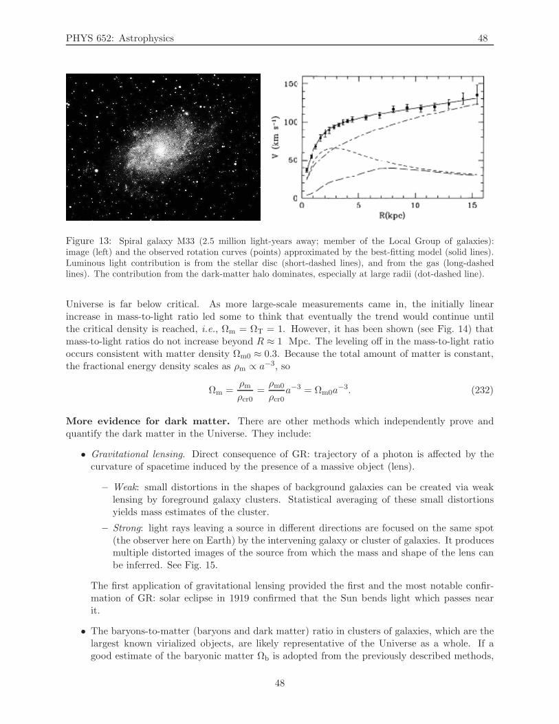
PHYS 652: Astrophysics 48
Figure 13: Spiral galaxy M33 (2.5 million light-years away; member of the Local Group of galaxies):image (left) and the observed rotation curves (points) approximated by the best-fitting model (solid lines).Luminous light contribution is from the stellar disc (short-dashed lines), and from the gas (long-dashedlines). The contribution from the dark-matter halo dominates, especially at large radii (dot-dashed line).
Universe is far below critical. As more large-scale measurements came in, the initially linearincrease in mass-to-light ratio led some to think that eventually the trend would continue untilthe critical density is reached, i.e., Ωm = ΩT = 1. However, it has been shown (see Fig. 14) thatmass-to-light ratios do not increase beyond R ≈ 1 Mpc. The leveling off in the mass-to-light ratiooccurs consistent with matter density Ωm0 ≈ 0.3. Because the total amount of matter is constant,the fractional energy density scales as ρm ∝ a−3, so
Ωm =ρmρcr0
=ρm0
ρcr0a−3 = Ωm0a
−3. (232)
More evidence for dark matter. There are other methods which independently prove andquantify the dark matter in the Universe. They include:
• Gravitational lensing. Direct consequence of GR: trajectory of a photon is affected by thecurvature of spacetime induced by the presence of a massive object (lens).
– Weak: small distortions in the shapes of background galaxies can be created via weaklensing by foreground galaxy clusters. Statistical averaging of these small distortionsyields mass estimates of the cluster.
– Strong: light rays leaving a source in different directions are focused on the same spot(the observer here on Earth) by the intervening galaxy or cluster of galaxies. It producesmultiple distorted images of the source from which the mass and shape of the lens canbe inferred. See Fig. 15.
The first application of gravitational lensing provided the first and the most notable confir-mation of GR: solar eclipse in 1919 confirmed that the Sun bends light which passes nearit.
• The baryons-to-matter (baryons and dark matter) ratio in clusters of galaxies, which are thelargest known virialized objects, are likely representative of the Universe as a whole. If agood estimate of the baryonic matter Ωb is adopted from the previously described methods,
48
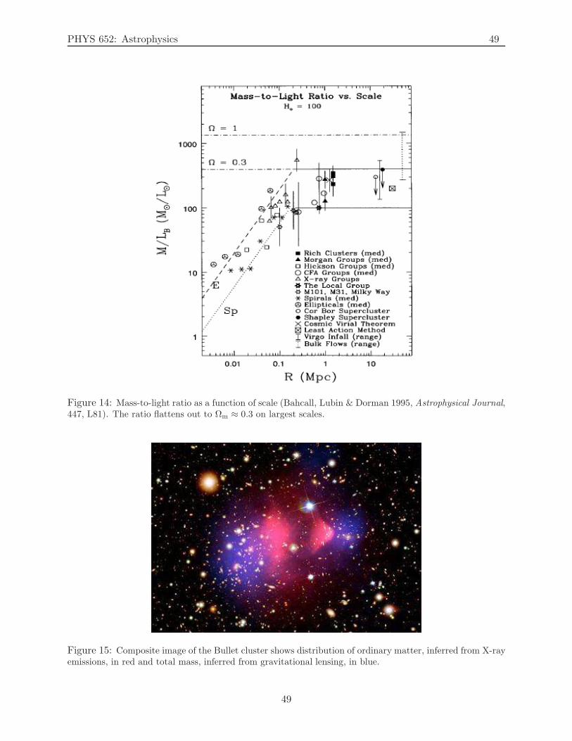
PHYS 652: Astrophysics 49
Figure 14: Mass-to-light ratio as a function of scale (Bahcall, Lubin & Dorman 1995, Astrophysical Journal,447, L81). The ratio flattens out to Ωm ≈ 0.3 on largest scales.
Figure 15: Composite image of the Bullet cluster shows distribution of ordinary matter, inferred from X-rayemissions, in red and total mass, inferred from gravitational lensing, in blue.
49
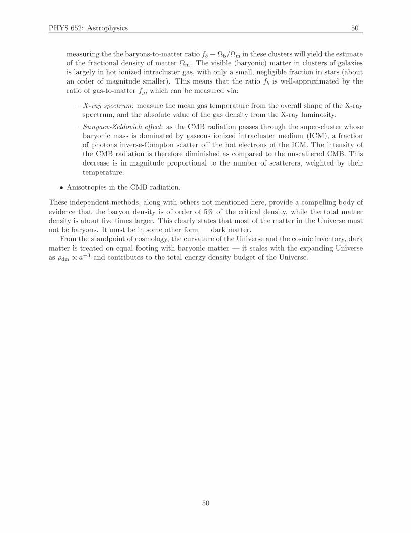
PHYS 652: Astrophysics 50
measuring the the baryons-to-matter ratio fb ≡ Ωb/Ωm in these clusters will yield the estimateof the fractional density of matter Ωm. The visible (baryonic) matter in clusters of galaxiesis largely in hot ionized intracluster gas, with only a small, negligible fraction in stars (aboutan order of magnitude smaller). This means that the ratio fb is well-approximated by theratio of gas-to-matter fg, which can be measured via:
– X-ray spectrum: measure the mean gas temperature from the overall shape of the X-rayspectrum, and the absolute value of the gas density from the X-ray luminosity.
– Sunyaev-Zeldovich effect: as the CMB radiation passes through the super-cluster whosebaryonic mass is dominated by gaseous ionized intracluster medium (ICM), a fractionof photons inverse-Compton scatter off the hot electrons of the ICM. The intensity ofthe CMB radiation is therefore diminished as compared to the unscattered CMB. Thisdecrease is in magnitude proportional to the number of scatterers, weighted by theirtemperature.
• Anisotropies in the CMB radiation.
These independent methods, along with others not mentioned here, provide a compelling body ofevidence that the baryon density is of order of 5% of the critical density, while the total matterdensity is about five times larger. This clearly states that most of the matter in the Universe mustnot be baryons. It must be in some other form — dark matter.
From the standpoint of cosmology, the curvature of the Universe and the cosmic inventory, darkmatter is treated on equal footing with baryonic matter — it scales with the expanding Universeas ρdm ∝ a−3 and contributes to the total energy density budget of the Universe.
50
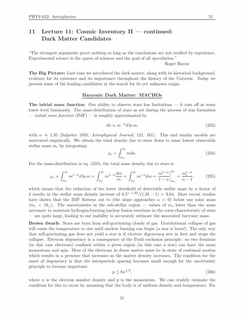
PHYS 652: Astrophysics 51
11 Lecture 11: Cosmic Inventory II — continued:Dark Matter Candidates
“The strongest arguments prove nothing so long as the conclusions are not verified by experience.Experimental science is the queen of sciences and the goal of all speculation.”
Roger Bacon
The Big Picture: Last time we introduced the dark matter, along with its historical background,evidence for its existence and its importance throughout the history of the Universe. Today wepresent some of the leading candidates in the search for its yet unknown origin.
Baryonic Dark Matter: MACHOs
The initial mass function. Our ability to observe stars has limitations — it cuts off at somelower level luminosity. The mass-distribution of stars as set during the process of star formation— initial mass function (IMF) — is roughly approximated by
dn ∝ m−αd lnm, (233)
with α ≈ 1.35 (Salpeter 1955, Astrophysical Journal, 121, 161). This and similar models aremotivated empirically. We obtain the total density due to stars down to some lowest observablestellar mass mc by integrating:
ρs =
∫ ∞
mc
mdn. (234)
For the mass-distribution in eq. (233), the total mass density due to stars is
ρs ∝∫ ∞
mc
m1−αd lnm =
∫ ∞
mc
m1−αdm
m=
∫ ∞
mc
m−αdm =m1−α
1− α
∣
∣
∣
∣
∞
mc
=m1−αc
α− 1, (235)
which means that the reduction of the lower threshold of detectable stellar mass by a factor of2 results in the stellar mass density increase of 0.51−1.35/(1.35 − 1) = 3.64. More recent studieshave shown that the IMF flattens out to (the slope approaches α = 0) below one solar mass(mc < M⊙). The uncertainties in the sub-stellar region — values of ms lower than the massnecessary to maintain hydrogen-burning nuclear fusion reactions in the cores characteristic of stars— are quite large, leading to our inability to accurately estimate the associated baryonic mass.
Brown dwarfs. Stars are born from self-gravitating clouds of gas. Gravitational collapse of gaswill cause the temperature to rise until nuclear burning can begin (a star is born!). The only waythat self-gravitating gas does not yield a star is if electron degeneracy sets in first and stops thecollapse. Electron degeneracy is a consequence of the Pauli exclusion principle: no two fermions(in this case electrons) confined within a given region (in this case a star) can have the samemomentum and spin. Most of the electrons in dense matter must be in state of continual motionwhich results in a pressure that increases as the matter density increases. The condition for theonset of degeneracy is that the interparticle spacing becomes small enough for the uncertaintyprinciple to become important:
p ≤ ~n1/3, (236)
where n is the electron number density and p is the momentum. We can crudely estimate thecondition for this to occur by assuming that the body is of uniform density and temperature. For
51
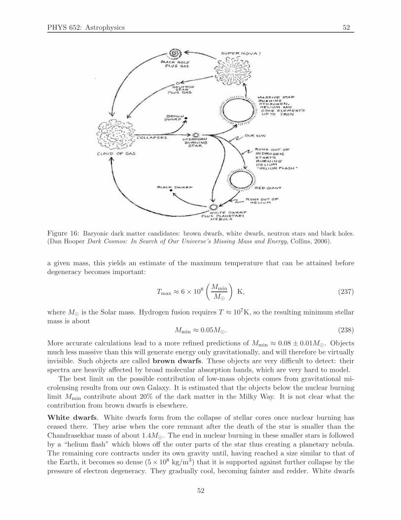
PHYS 652: Astrophysics 52
Figure 16: Baryonic dark matter candidates: brown dwarfs, white dwarfs, neutron stars and black holes.(Dan Hooper Dark Cosmos: In Search of Our Universe’s Missing Mass and Energy, Collins, 2006).
a given mass, this yields an estimate of the maximum temperature that can be attained beforedegeneracy becomes important:
Tmax ≈ 6× 10⁸(
Mmin
M⊙
)
K, (237)
where M⊙ is the Solar mass. Hydrogen fusion requires T ≈ 107K, so the resulting minimum stellarmass is about
Mmin ≈ 0.05M⊙. (238)
More accurate calculations lead to a more refined predictions of Mmin ≈ 0.08 ± 0.01M⊙. Objectsmuch less massive than this will generate energy only gravitationally, and will therefore be virtuallyinvisible. Such objects are called brown dwarfs. These objects are very difficult to detect: theirspectra are heavily affected by broad molecular absorption bands, which are very hard to model.
The best limit on the possible contribution of low-mass objects comes from gravitational mi-crolensing results from our own Galaxy. It is estimated that the objects below the nuclear burninglimit Mmin contribute about 20% of the dark matter in the Milky Way. It is not clear what thecontribution from brown dwarfs is elsewhere.
White dwarfs. White dwarfs form from the collapse of stellar cores once nuclear burning hasceased there. They arise when the core remnant after the death of the star is smaller than theChandrasekhar mass of about 1.4M⊙. The end in nuclear burning in these smaller stars is followedby a “helium flash” which blows off the outer parts of the star thus creating a planetary nebula.The remaining core contracts under its own gravity until, having reached a size similar to that ofthe Earth, it becomes so dense (5× 10⁸ kg/m3) that it is supported against further collapse by thepressure of electron degeneracy. They gradually cool, becoming fainter and redder. White dwarfs
52
PHYS 652: Astrophysics 53
may constitute about 30% of the stars in solar neighborhood, but because of their low luminosity(typically 10−3 to 10−4 of the Sun’s) they are very inconspicuous.
Neutron stars. Neutron stars form from the collapse of stellar cores once nuclear burning hasceased there. They arise when the core remnant after the death of the star is larger than theChandrasekhar mass of about 1.4M⊙, but still smaller than about 2M⊙. The neutron stars whichare created from core remnants with M > 2M⊙ will eventually collapse further into a black hole.The end in nuclear burning in larger stars is followed by a “supernova”. The remaining corecontracts under its own gravity until, at a density of about 1017 kg/m3, electrons and protonsare so closely packed that they combine to form neutrons. The resultant object, consisting only ofneutrinos, is supported against further gravitational collapse by the pressure of neutron degeneracy.A typical neutron star, with a mass little greater than the mass of the Sun, has a diameter of onlyabout 30 km. (Pulsars are spinning magnetized neutron stars.)
Black holes. Black holes form from the collapse of stellar cores once nuclear burning has ceasedthere. They arise when the core remnant after the death of the star is larger than 2M⊙. Whenneutron degeneracy becomes insufficient to support the neutron star from collapsing, its radiusradius shrinks to below critical size known as the Schwarzschild radius.
All of these compact (sub-)stellar objects are examples of MAssive Compact Halo Objects (MA-CHOs), objects which we cannot directly see. Therefore, they are a form of dark matter. However,even with their contributions added to the visible baryonic matter, the total content of matter inthe Universe is still significantly short.
Non-Baryonic Dark Matter: WIMPs
Although we presented a strong case that at least a portion of the dark matter content isbaryonic, there exists strong cosmological evidence that the dark matter consists of weakly in-teracting relic particles. The strongest case is built by primordial nucleosynthesis, or Big BangNucleosynthesis (BBN), which estimates that a baryonic contribution to the total energy densityis Ωb0 ≈ 0.0125h−2. This is the contribution of the protons and neutrons that interacted to fix thelight-element abundances at t ≈ 1 minute or so.
At the time of BBN, the Universe consisted of baryons (plus electrons, which are implicitlyincluded in the “baryonic matter”), photons and three species of neutrinos. To account for darkmatter, one can proceed in two ways from there: (i) neutrinos have mass; or (ii) there must existsome additional particle species that is a frozen-out relic from an earlier epoch.
A small neutrino mass would not affect the BBN, since the neutrinos are ultrarelativistic priorto matter–radiation equality. Other relic particles would have to be either very rare or extremelyweakly coupled (even more weakly than neutrinos) in order not to effect the BBN. Either alternativewould produce the dark matter which is collisionless, which is the main argument in favor ofnonbaryonic dark matter: the clustering power spectrum appears to be free of oscillatory featuresexpected from the gravitational growth of perturbations in matter that is able to support soundwaves.
There are a number of different Weakly Interacting Massive Particles (WIMPs) candidates forthe dark matter particle. They are called “weakly interacting” because they interact only by weakinteraction and gravity, and are therefore notoriously difficult to detect.
• Massive neutrinos. The most obvious species of nonbaryonic dark matter to consider asa dark matter particle candidate is a massive neutrino. Because neutrinos are very weaklyinteracting, it is still unclear what the mass of neutrinos may be. Recent experiments only
53
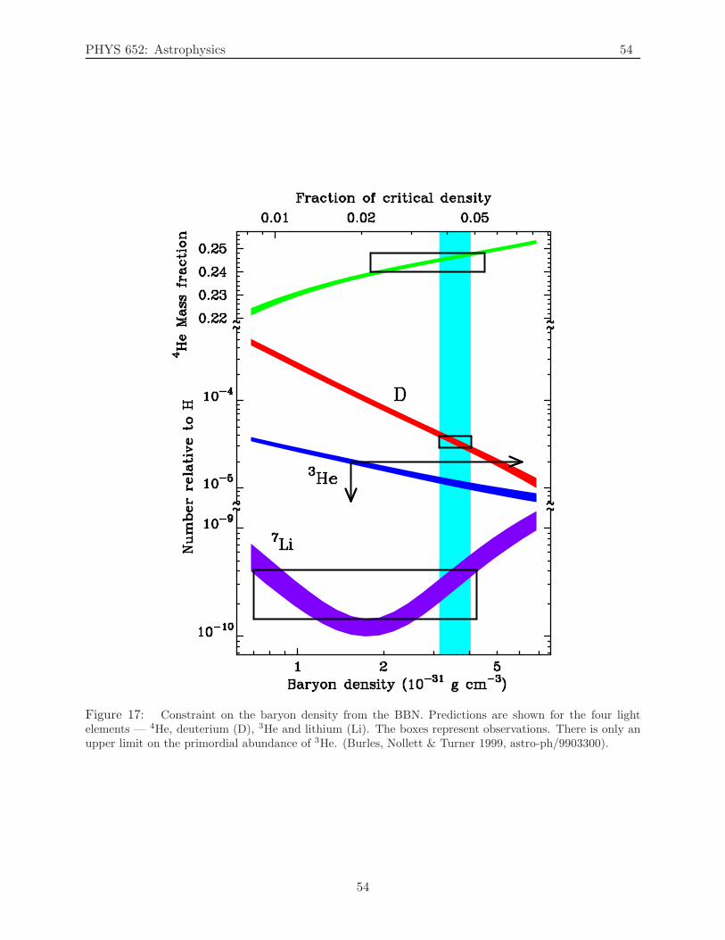
PHYS 652: Astrophysics 54
Figure 17: Constraint on the baryon density from the BBN. Predictions are shown for the four lightelements — 4He, deuterium (D), 3He and lithium (Li). The boxes represent observations. There is only anupper limit on the primordial abundance of 3He. (Burles, Nollett & Turner 1999, astro-ph/9903300).
54
PHYS 652: Astrophysics 55
put constraints on the difference of squares of masses of two flavors of neutrinos.
• Supersymmetric particles. Particles which are part of the theory of supersymmetry(SUSY), and which are yet to be detected are also considered as dark matter candidates.Among them are particles like axions and neutralinos.
There is another categorization of WIMPs, which is more descriptive of their nature: hot and colddark matter.
Hot dark matter (HDM). Hot dark matter particles — neutrinos — decouple when they arerelativistic, and have a number density roughly equal to that of photons. These low-mass relicsare hot in the sense of possessing large quasi-thermal velocities. These velocities were larger athigh redshifts, which resulted in major effects on the development of self-gravitating structures.The structure forms by fragmentation — top-down — with largest super-clusters forming first inflat sheets and subsequently fragmenting into smaller pieces to form smaller structures — clusters,galaxies and stars.
The predictions of HDM matter strongly disagree with observations.
Cold dark matter (CDM). Most cosmologists favor the CDM theory as a description of how theUniverse went from a smooth initial state at early times (as demonstrated by the CMB radiation)to the lumpy distribution of galaxies and clusters of galaxies that we observe today.
In the CDM theory, the structure grows hierarchically — bottom-up — with small objectscollapsing first and merging in a continuous hierarchy to form more and more massive objects —stars, galaxies, cluster, super-clusters. The CDM clusters hierarchically with the number countgrowing with the decreasing size of halos.
The predictions of CDM generally agrees with observations. There are two important discrep-ancies between predictions of the CDM paradigm and observations of galaxies and their clustering,thereby creating a potential crisis for the CDM picture:
• The cuspy halo problem: CDM predicts that the central density slopes of galaxies are muchsteeper than they have been observed.
• The missing satellites problem: the CDM predicts large number of small dwarf galaxies aboutone thousandth the mass of the Milky Way. The number of these dwarf galaxies and theirsmall halos is orders of magnitude lower than expected from simulations.
55
PHYS 652: Astrophysics 56
12 Lecture 12: Cosmic Inventory III: Dark Energy
“It is far better to grasp the Universe as it really is than to persist in delusion, however satisfyingand reassuring.”
Carl Sagan
The Big Picture: For the last couple of lectures we talked about the dark matter — its historicalbackground, evidence for its existence, its importance for the history of the Universe, as well assome of the leading candidates in the search for its yet unknown origin. Today we are going todiscuss the dark energy — evidence for its existence, its implication for the structure and evolutionof the Universe and some alternatives.
Dark Energy
The notion of a “cosmological constant” has been floating around since the time of Newton(see Article 2). However, it is only recently that it has obtained firm footing with theoretical andobservational evidence. There are two sets of evidence which support the existence of additionalenergy density — “dark energy” — due to cosmological constant:
1. Budgetary shortfall. The total energy density of the Universe is very close to critical, assuggested both: (i) theoretically from the inflation in the early Universe; and (ii) observation-ally from the anisotropies of the CMB radiation. However, the observations can only accountfor about a third of the total critical energy density. The remaining, unaccounted, two thirdsof the density in the Universe must be in some smooth, unclustered form — dark energy.
2. Theoretical distance-redshift relations. Given the energy composition of the Universe,one can put together graphs of theoretical distance (luminosity for instance) versus redshift,which can be verified observationally. In 1998, two groups (Riess et al. 1998, Astronom-ical Journal, 116, 1009; Perlmutter et al. 1999, Astrophysical Journal 517, 565) observingsupernovae reported direct evidence for the dark energy.
The evidence is based on the difference between the dependence of the luminosity distancedL on redshift z in matter-dominated Universe and in the dark energy-dominated Universe.These dependences are given in Fig. 10. The graph shows that the luminosity density distanceis larger for objects at higher redshifts in a dark energy-dominated Universe. This meansthat the objects of fixed intrinsic brightness (“standard candles”) will appear dimmer in theUniverse composed of predominantly dark matter.
Using Luminosity Distance Vs. Redshift Graphs to Detect Dark Energy
Let us illustrate how this direct evidence of the dark energy was obtained from the measurementsof the luminosity distance for Type Ia supernovae, which are considered “standard candles” — theirintrinsic (absolute) luminosity are nearly identical.
The luminosity distance dL given by eq. (189)
dL =χ
a, (239)
56
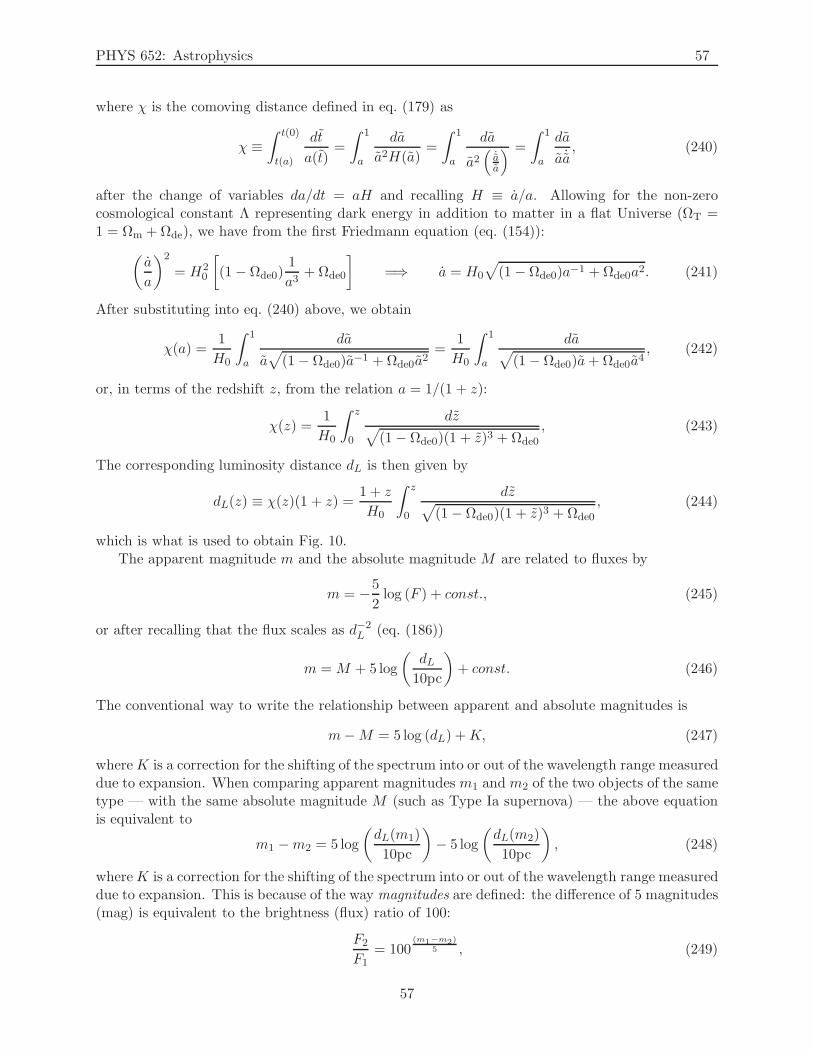
PHYS 652: Astrophysics 57
where χ is the comoving distance defined in eq. (179) as
χ ≡∫ t(0)
t(a)
dt
a(t)=
∫ 1
a
da
a2H(a)=
∫ 1
a
da
a2(
˙aa
) =
∫ 1
a
da
a ˙a, (240)
after the change of variables da/dt = aH and recalling H ≡ a/a. Allowing for the non-zerocosmological constant Λ representing dark energy in addition to matter in a flat Universe (ΩT =1 = Ωm +Ωde), we have from the first Friedmann equation (eq. (154)):
(
a
a
)2
= H20
[
(1− Ωde0)1
a3+Ωde0
]
=⇒ a = H0
√
(1− Ωde0)a−1 +Ωde0a2. (241)
After substituting into eq. (240) above, we obtain
χ(a) =1
H0
∫ 1
a
da
a√
(1− Ωde0)a−1 +Ωde0a2=
1
H0
∫ 1
a
da√
(1− Ωde0)a+Ωde0a4, (242)
or, in terms of the redshift z, from the relation a = 1/(1 + z):
χ(z) =1
H0
∫ z
0
dz√
(1− Ωde0)(1 + z)3 +Ωde0
, (243)
The corresponding luminosity distance dL is then given by
dL(z) ≡ χ(z)(1 + z) =1 + z
H0
∫ z
0
dz√
(1−Ωde0)(1 + z)3 +Ωde0
, (244)
which is what is used to obtain Fig. 10.The apparent magnitude m and the absolute magnitude M are related to fluxes by
m = −5
2log (F ) + const., (245)
or after recalling that the flux scales as d−2L (eq. (186))
m = M + 5 log
(
dL10pc
)
+ const. (246)
The conventional way to write the relationship between apparent and absolute magnitudes is
m−M = 5 log (dL) +K, (247)
whereK is a correction for the shifting of the spectrum into or out of the wavelength range measureddue to expansion. When comparing apparent magnitudes m1 and m2 of the two objects of the sametype — with the same absolute magnitude M (such as Type Ia supernova) — the above equationis equivalent to
m1 −m2 = 5 log
(
dL(m1)
10pc
)
− 5 log
(
dL(m2)
10pc
)
, (248)
whereK is a correction for the shifting of the spectrum into or out of the wavelength range measureddue to expansion. This is because of the way magnitudes are defined: the difference of 5 magnitudes(mag) is equivalent to the brightness (flux) ratio of 100:
F2
F1= 100
(m1−m2)5 , (249)
57
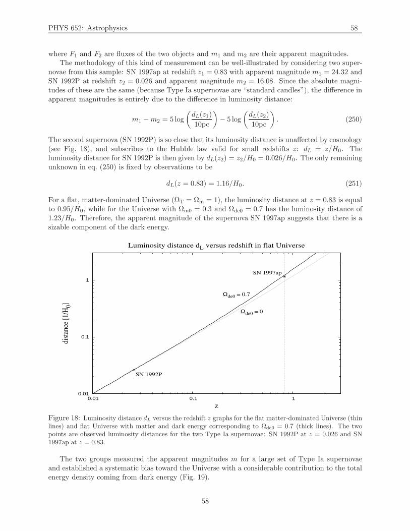
PHYS 652: Astrophysics 58
where F1 and F2 are fluxes of the two objects and m1 and m2 are their apparent magnitudes.The methodology of this kind of measurement can be well-illustrated by considering two super-
novae from this sample: SN 1997ap at redshift z1 = 0.83 with apparent magnitude m1 = 24.32 andSN 1992P at redshift z2 = 0.026 and apparent magnitude m2 = 16.08. Since the absolute magni-tudes of these are the same (because Type Ia supernovae are “standard candles”), the difference inapparent magnitudes is entirely due to the difference in luminosity distance:
m1 −m2 = 5 log
(
dL(z1)
10pc
)
− 5 log
(
dL(z2)
10pc
)
. (250)
The second supernova (SN 1992P) is so close that its luminosity distance is unaffected by cosmology(see Fig. 18), and subscribes to the Hubble law valid for small redshifts z: dL = z/H0. Theluminosity distance for SN 1992P is then given by dL(z2) = z2/H0 = 0.026/H0. The only remainingunknown in eq. (250) is fixed by observations to be
dL(z = 0.83) = 1.16/H0. (251)
For a flat, matter-dominated Universe (ΩT = Ωm = 1), the luminosity distance at z = 0.83 is equalto 0.95/H0, while for the Universe with Ωm0 = 0.3 and Ωde0 = 0.7 has the luminosity distance of1.23/H0. Therefore, the apparent magnitude of the supernova SN 1997ap suggests that there is asizable component of the dark energy.
0.01
0.1
1
0.01 0.1 1
dist
ance
[1/
H0]
z
Luminosity distance dL versus redshift in flat Universe
Ωde0 = 0
Ωde0 = 0.7
SN 1992P
SN 1997ap
Figure 18: Luminosity distance dL versus the redshift z graphs for the flat matter-dominated Universe (thinlines) and flat Universe with matter and dark energy corresponding to Ωde0 = 0.7 (thick lines). The twopoints are observed luminosity distances for the two Type Ia supernovae: SN 1992P at z = 0.026 and SN1997ap at z = 0.83.
The two groups measured the apparent magnitudes m for a large set of Type Ia supernovaeand established a systematic bias toward the Universe with a considerable contribution to the totalenergy density coming from dark energy (Fig. 19).
58
PHYS 652: Astrophysics 59
The measurement of Type Ia supernovae conducted by the two teams led to the constraints onthe Universe presented in Fig. 20. The two free parameters are the relative content of matter (ΩM)and the dark energy modeled as a cosmological constant or vacuum energy (ΩΛ), which is only oneof the possibly ways to model it. Figure 20 seems to confidently rule out the flat matter-dominatedUniverse (ΩΛ = 0, ΩM = 1), as well as the open Universe with only matter (ΩM = 0.3).
Figure 21 shows the age of the Universe and its acceleration for different ratios of ΩΛ and ΩM.Figure 20 allows for a great deal of freedom — the shaded, most probable region is quite
elongated allowing for a broad range of viable ratios.In order to allow for other forms of dark energy, we allow for dark energy density to be time-
dependent (and not due to the cosmological constant Λ). Equation of state P = P (ρ) for darkenergy must obey the Friedmann’s second equation (eq. (101b)):
dρ
dt+ 3 (ρ+ P )
a
a= 0. (252)
For time-independent dark energy, i.e. due to cosmological constant Λ, the equation of state is
P = −ρ. (253)
Earlier we introduced a parameter w in the equation of state:
w ≡ P
ρ, (254)
where w = 0 for matter, w = 1/3 for radiation and w = −1 for dark energy due to cosmologicalconstant (see Table 3). The two studies of supernovae also computed the likelihood regions in the(ΩM, w) space in the case of flat Universe. Figure 22 shows that the cosmological constant (w = −1)is allowed, but not the only possibility.
To compute how the time-dependent dark energy density, as denoted by w = w(t), or equiva-lently w = w(a), evolves with the expanding Universe, we can solve eq. (252) with w = w(a):
dρ
dt= −3 [ρ+ w(a)ρ]
a
a= −3ρ [1 + w(a)]
da
adt
=⇒∫ a dρ
ρ= −3
∫ a[
1 + w(a′)] da′
a′
=⇒ ρ ∝ exp
−3
∫ a[
1 + w(a′)] da′
a′
. (255)
If w = const., then
ρ ∝ exp
−3 (1 + w)
∫ a da′
a′
= exp −3 (1 + w) ln a = exp
ln a−3(1+w)
= a−3(1+w), (256)
which matches ρ ∝ a−3 for w = 0 (matter: dust approximation P = 0), ρ ∝ a−4 for w = 1/3(radiation: perfect fluid approximation P = ρ/3) and ρ ∝ const. for w = −1 (cosmological constantΛ: P = −ρ).
There are several “popular” values of w for the dark energy:
• w < −1/3: quintessence,
• w = −1: cosmological constant Λ,
59
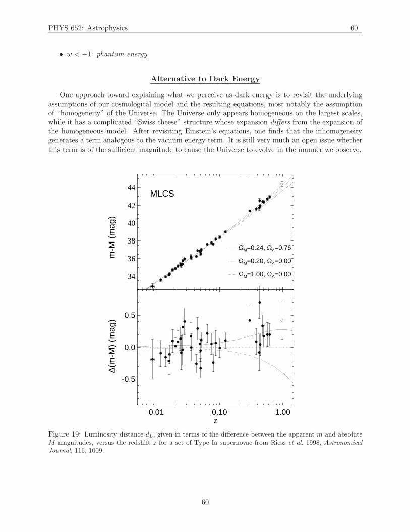
PHYS 652: Astrophysics 60
• w < −1: phantom energy.
Alternative to Dark Energy
One approach toward explaining what we perceive as dark energy is to revisit the underlyingassumptions of our cosmological model and the resulting equations, most notably the assumptionof “homogeneity” of the Universe. The Universe only appears homogeneous on the largest scales,while it has a complicated “Swiss cheese” structure whose expansion differs from the expansion ofthe homogeneous model. After revisiting Einstein’s equations, one finds that the inhomogeneitygenerates a term analogous to the vacuum energy term. It is still very much an open issue whetherthis term is of the sufficient magnitude to cause the Universe to evolve in the manner we observe.
34
36
38
40
42
44
ΩM=0.24, ΩΛ=0.76
ΩM=0.20, ΩΛ=0.00
ΩM=1.00, ΩΛ=0.00
m-M
(m
ag)
MLCS
0.01 0.10 1.00z
-0.5
0.0
0.5
∆(m
-M)
(mag
)
Figure 19: Luminosity distance dL, given in terms of the difference between the apparent m and absoluteM magnitudes, versus the redshift z for a set of Type Ia supernovae from Riess et al. 1998, AstronomicalJournal, 116, 1009.
60
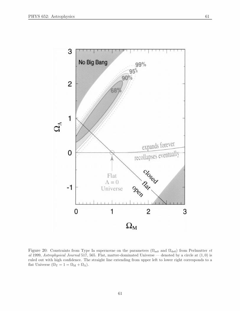
PHYS 652: Astrophysics 61
Figure 20: Constraints from Type Ia supernovae on the parameters (Ωm0 and Ωde0) from Perlmutter etal 1999, Astrophysical Journal 517, 565. Flat, matter-dominated Universe — denoted by a circle at (1, 0) isruled out with high confidence. The straight line extending from upper left to lower right corresponds to aflat Universe (ΩT = 1 = ΩM +ΩΛ).
61
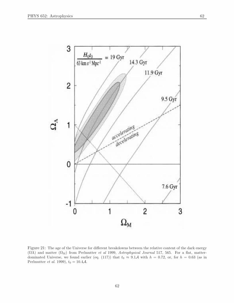
PHYS 652: Astrophysics 62
Figure 21: The age of the Universe for different breakdowns between the relative content of the dark energy(ΩΛ) and matter (ΩM) from Perlmutter et al 1999, Astrophysical Journal 517, 565. For a flat, matter-dominated Universe, we found earlier (eq. (117)) that t0 ≈ 9.1A with h = 0.72, or, for h = 0.63 (as inPerlmutter et al. 1999), t0 = 10.4A.
62
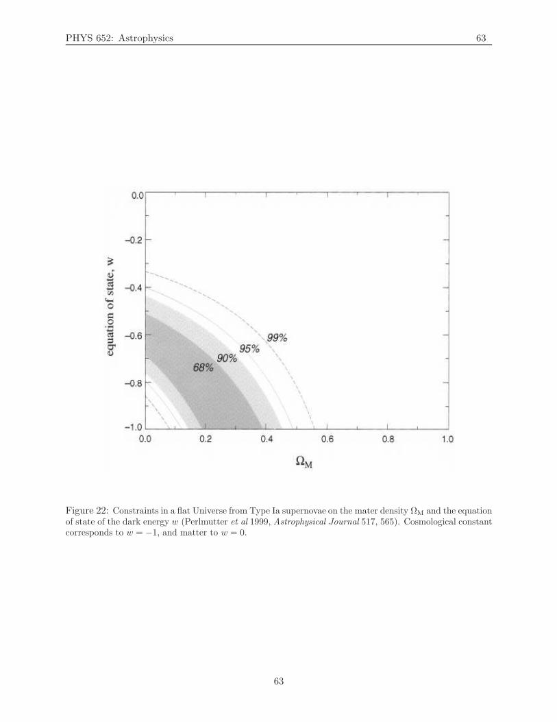
PHYS 652: Astrophysics 63
Figure 22: Constraints in a flat Universe from Type Ia supernovae on the mater density ΩM and the equationof state of the dark energy w (Perlmutter et al 1999, Astrophysical Journal 517, 565). Cosmological constantcorresponds to w = −1, and matter to w = 0.
63
PHYS 652: Astrophysics 64
13 Lecture 13: History of the Very Early Universe
“The Universe is full of magical things, patiently waiting for our wits to grow sharper.”Eden Phillpots
The Big Picture: Today we are going to outline the standard model of the Universe in the firstfew minutes following the hot Big Bang. These earliest epochs in the evolution of the Universeare still inadequately understood. As we move away from the Big Bang, our understanding of thephysical epochs of the Universe becomes increasingly better understood.
Keeping Track of Universe’s History
The different times in the history of the Universe can be tracked by any of the several quantitieswhich change monotonically throughout: age of the Universe t, scale factor a, redshift (as we observeit today) z and temperature of the CMB radiation T (currently measured at ≈ 2.7 K).
From eq. (205)
ργ =π2
15T 4γ , (257)
and the result derived from Friedmann’s second equation that the radiation scales as
ργ ∝ a−4, (258)
we obtain thatTγ(a) ∝ a−1, (259)
which, combined with the current measurement of the temperature of the CMB radiation
Tγ0 = Tγ(a = 1) ≈ 2.7K, (260)
yieldsTγ(a) ≈ 2.7a−1. (261)
To relate this to the age of the Universe t, one can explicitly solve integrals for a(t) and substitutein eq. (261).
The mutual relationship between the quantities t, z, a and Tγ is given in Table 5.It is beneficial to relate directly — albeit crudely — the temperature T and the age of the
Universe t. This can only be analytically only for matter-dominated or radiation-dominated Uni-verse, as we have done in Lecture 5. (Relating the scale factor a and the age of the Universe t in amore general case when Universe has matter, radiation and the cosmological constant (as vacuumenergy) requires solving the integral given in Table 5 for t(a) and inverting it. This can only bedone numerically). Therefore, as a rough approximation, let us recall:
1. flat, matter-dominated Universe [eq. (115)]: a(t) =(
3H02
)2/3t2/3,
2. flat, radiation-dominated Universe [eq. (119)]: a(t) = (2H0)1/2 t1/2,
where
H0 = 100h km sec−1Mpc−1 = 100h
(
1000m
1km
)(
1Mpc
3.0856 × 10²²m
)
km sec−1Mpc−1
H0 ≈ 3.24h × 10−18sec−1 ≈ 2.3 × 10⁻¹⁸sec−1, (262)
with h ≈ 0.72. Therefore, for the two approximations, we have:
64
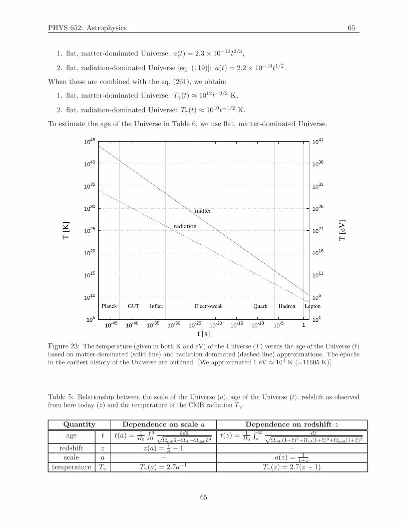
PHYS 652: Astrophysics 65
1. flat, matter-dominated Universe: a(t) = 2.3× 10⁻¹²t2/3,
2. flat, radiation-dominated Universe [eq. (119)]: a(t) = 2.2× 10⁻¹⁰t1/2.
When these are combined with the eq. (261), we obtain:
1. flat, matter-dominated Universe: Tγ(t) ≈ 1012t−2/3 K,
2. flat, radiation-dominated Universe: Tγ(t) ≈ 1010t−1/2 K.
To estimate the age of the Universe in Table 6, we use flat, matter-dominated Universe.
105
1010
1015
1020
1025
1030
1035
1040
1045
110-510-1010-1510-2010-2510-3010-3510-4010-45101
106
1011
1016
1021
1026
1031
1036
1041
T [
K]
T [
eV]
t [s]
matter
radiation
Planck GUT Inflat. Electroweak Quark Hadron Lepton
Figure 23: The temperature (given in both K and eV) of the Universe (T ) versus the age of the Universe (t)based on matter-dominated (solid line) and radiation-dominated (dashed line) approximations. The epochsin the earliest history of the Universe are outlined. [We approximated 1 eV ≈ 104 K (=11605 K)].
Table 5: Relationship between the scale of the Universe (a), age of the Universe (t), redshift as observedfrom here today (z) and the temperature of the CMB radiation Tγ .
Quantity Dependence on scale a Dependence on redshift z
age t t(a) = 1H0
∫ a0
ada√Ωm0a+Ωr0+Ωde0a4
t(z) = 1H0
∫∞z
dz√Ωm0(1+z)5+Ωr0(1+z)6+Ωde0(1+z)2
redshift z z(a) = 1a − 1 –
scale a – a(z) = 11+z
temperature Tγ Tγ(a) = 2.7a−1 Tγ(z) = 2.7(z + 1)
65
PHYS 652: Astrophysics 66
The Big Bang: t = 0 s
Extrapolation of the expansion of the Universe backwards in time using general relativity yields aninfinite density and temperature at a finite time in the past. This singularity signals the breakdownof GR. How closely we can extrapolate towards the singularity is debated — certainly not earlierthan the Planck epoch. The early hot, dense phase is itself referred to as “the Big Bang”, and isconsidered the “birth” of our Universe — The Beginning.
The discussion about the nature, cause and origin of the Big Bang itself is untestable and assuch quickly enters the waters of metaphysics and theology.
The Planck Epoch: 0 < t ≤ 10−43
s
The Planck epoch is the earliest period of time in the history of the Universe, spanning thebrief time immediately following the Big Bang during which the quantum effects of gravity weresignificant.
In order to compute the time-scale over which quantum effects dominate (barring the existenceof branes which would circumvent them), we use dimensional analysis:
effects constant value units
Relativity c 3× 10¹⁰ cms
Quantum mechanics h 6.63× 10⁻²⁷ g cm2
s
Gravitation G 6.67 × 10⁻⁸ cm3
gs2
We need to find the way to combine the constants above to obtain the the relevant time scale:
cAhBGD = s,
=⇒(cm
s
)A(
gcm2
s
)B (cm3
gs2
)D
= s,
[cm] : A +2B +3D = 0[g] : +B −D = 0[s] : −A −B −2D = 1
Solution A = −52 B = 1
2 D = 12 =⇒ tP = c
52h
12G
12 ,
The time scale for quantum gravity, the Planck time tP , is therefore
tP ≡√
hG
c5, (263)
which numerically is equal to
tP =
[
(6.63 × 10⁻²⁷)(6.67 × 10⁻⁸)
(3× 10¹⁰)5
]1/2
≈ 10−43s. (264)
If the supersymmetry is correct, then during this time the four fundamental forces — electro-magnetism, weak force, strong force and gravity — all have the same strength, so they are possiblyunified into one fundamental force. Our understanding of this early epoch is still quite tenuous,awaiting a happy marriage of quantum mechanics and relativistic gravity.
66
PHYS 652: Astrophysics 67
Grand Unification Epoch: 10−43
s ≤ t ≤ 10−36
s
Assuming the existence of a Grand Unification Theory (GUT), the Grand Unification Epochwas the period in the evolution of the early Universe following the Planck epoch, in which thetemperature of the Universe was comparable to the characteristic temperatures of GUTs. If thegrand unification energy is taken to be 1015 GeV, this corresponds to temperatures higher than1027 K. During this period, three of the four fundamental interactions — electromagnetism, thestrong interaction, and the weak interaction — were unified as the electronuclear force. Gravity hadseparated from the electronuclear force at the end of the Planck era. During the Grand UnificationEpoch, physical characteristics such as mass, charge, flavor and color charge were meaningless.
The Grand Unification Epoch ended at approximately 10−36s after the Big Bang. At this point,the strong force separated from the other fundamental forces.
Inflationary Epoch: 10−36
s ≤ t ≤ 10−32
s
The Inflationary Epoch was the period in the evolution of the early Universe when, accordingto inflation theory, the Universe underwent an extremely rapid exponential expansion. This rapidexpansion increased the linear dimensions of the early Universe by a factor of at least 1026 (andpossibly a much larger factor), and so increased its volume by a factor of at least 1078. At thistime, the strong force started to separate from the electroweak interaction.
The expansion is thought to have been triggered by the phase transition that marked the endof the preceding Grand Unification Epoch at approximately 10−36s after the Big Bang. One of thetheoretical products of this phase transition was a scalar field called the inflation field. As thisfield settled into its lowest energy state throughout the Universe, it generated a repulsive force thatled to a rapid expansion of the fabric of spacetime. This expansion explains various properties ofthe current Universe that are difficult to account for without the Inflationary Epoch (flat Universe,horizon problem, magnetic monopoles).
The rapid expansion of spacetime meant that elementary particles remaining from the GrandUnification Epoch were now distributed very thinly across the Universe. However, the huge poten-tial energy of the inflation field was released at the end of the Inflationary Epoch, repopulating theUniverse with a dense, hot mixture of quarks, anti-quarks and gluons as it entered the ElectroweakEpoch.
Electroweak Epoch: 10−32
s ≤ t ≤ 10−12
s
The Electroweak Epoch was the period in the evolution of the early Universe when the temper-ature of the Universe was high enough to merge electromagnetism and the weak interaction into asingle electroweak interaction (≈ 100GeV ≈ 1015K). At approximately 10−32s after the Big Bangthe potential energy of the inflation field that had driven the inflation of the Universe during theInflationary Epoch was released, filling the Universe with a dense, hot quark-gluon plasma (reheat-ing). Particle interactions in this phase were energetic enough to create large numbers of exoticparticles, including W and Z bosons and Higgs bosons. As the Universe expanded and cooled,interactions became less energetic and when the Universe was about 10−12s old, W and Z bosonsceased to be created. The remaining W and Z bosons decayed quickly, and the weak interactionbecame a short-range force in the following Quark Epoch.
After the Inflationary Epoch, the physics of the Electroweak Epoch is less speculative and betterunderstood than for previous periods of the early Universe. The existence of W and Z bosons hasbeen demonstrated, and other predictions of electroweak theory have been experimentally verified.
67
PHYS 652: Astrophysics 68
Quark Epoch: 10−12
s ≤ t ≤ 10−6s
The Quark Epoch was the period in the evolution of the early Universe when the fundamentalinteractions of gravitation, electromagnetism, the strong interaction and the weak interaction hadtaken their present forms, but the temperature of the Universe was still too high to allow quarksto bind together to form hadrons. The Quark Epoch began approximately 10−12s after the BigBang, when the preceding Electroweak Epoch ended as the electroweak interaction separated intothe weak interaction and electromagnetism. During the Quark Epoch the Universe was filled with adense, hot quark-gluon plasma, containing quarks, gluons and leptons. Collisions between particleswere too energetic to allow quarks to combine into mesons or baryons. The Quark Epoch endedwhen the Universe was about 10−6s old, when the average energy of particle interactions had fallenbelow the binding energy of hadrons. The following period, when quarks became confined withinhadrons, is known as the Hadron Epoch.
Hadron Epoch: 10−6s ≤ t ≤ 1 s
The Hadron Epoch was the period in the evolution of the early Universe during which themass of the Universe was dominated by hadrons. It started approximately 10−6s after the BigBang, when the temperature of the Universe had fallen sufficiently to allow the quarks from thepreceding Quark Epoch to bind together into hadrons. Initially, the temperature was high enoughto allow the creation of hadron/anti-hadron pairs, which kept matter and anti-matter in thermalequilibrium. However, as the temperature of the Universe continued to fall, hadron/anti-hadronpairs were no longer produced. Most of the hadrons and anti-hadrons were then eliminated inannihilation reactions, leaving a small residue of hadrons. The elimination of anti-hadrons wascompleted by one second after the Big Bang, when the following Lepton Epoch began.
Lepton Epoch: 1 s ≤ t ≤ 3 min
From the time tP of quantum gravity up to the lepton era, the physics of the Universe isdominated by very high temperatures (> 1012 K) and therefore by high-energy particle physics.
• Muon annihilation:At sufficiently high temperatures, there is a pair production:
γ + γ → µ+ + µ−,
=⇒ photon energy → muon mass. (265)
This can persist only as long as kT ≈ 2mµc2:
T ≥ 2mµc2
k=
2(200me)c2
k=
2(2009.1 × 10−28)(3 × 10¹⁰)2
1.38 × 10−16= 2× 10¹²K. (266)
Therefore, muons annihilate at T ≈ 1012K.
• Electron/positron annihilation:The argument used for muon annihilation applies to electron-positron pair production
T ≥ 2mec2
k≈ 1010K, (267)
so, electrons and positrons annihilate at T ≈ 1010K.
68
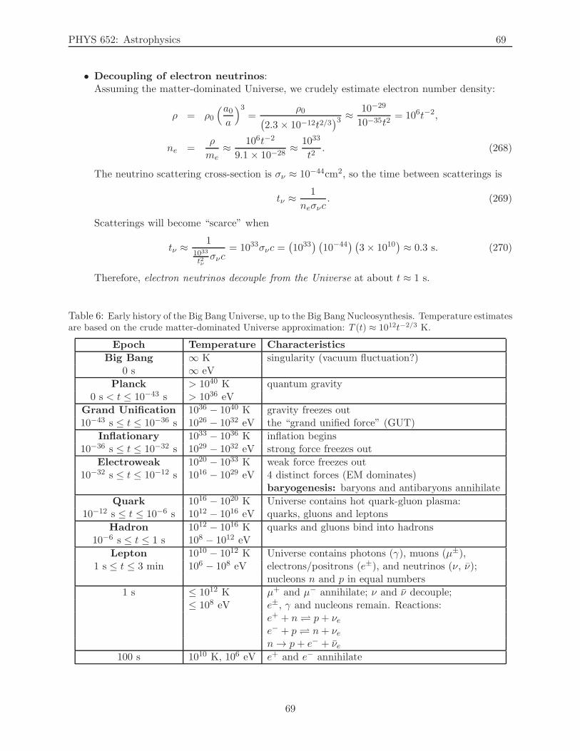
PHYS 652: Astrophysics 69
• Decoupling of electron neutrinos:Assuming the matter-dominated Universe, we crudely estimate electron number density:
ρ = ρ0
(a0a
)3=
ρ0(
2.3 × 10⁻¹²t2/3)3 ≈ 10−29
10−35t2= 106t−2,
ne =ρ
me≈ 106t−2
9.1 × 10⁻²⁸≈ 1033
t2. (268)
The neutrino scattering cross-section is σν ≈ 10−44cm2, so the time between scatterings is
tν ≈ 1
neσνc. (269)
Scatterings will become “scarce” when
tν ≈1
1033
t2νσνc
= 1033σνc =(
1033) (
10−44) (
3× 10¹⁰)
≈ 0.3 s. (270)
Therefore, electron neutrinos decouple from the Universe at about t ≈ 1 s.
Table 6: Early history of the Big Bang Universe, up to the Big Bang Nucleosynthesis. Temperature estimatesare based on the crude matter-dominated Universe approximation: T (t) ≈ 1012t−2/3 K.
Epoch Temperature Characteristics
Big Bang ∞ K singularity (vacuum fluctuation?)0 s ∞ eV
Planck > 1040 K quantum gravity0 s < t ≤ 10−43 s > 1036 eV
Grand Unification 1036 − 1040 K gravity freezes out10−43 s ≤ t ≤ 10−36 s 1026 − 1032 eV the “grand unified force” (GUT)
Inflationary 1033 − 1036 K inflation begins10−36 s ≤ t ≤ 10−32 s 1029 − 1032 eV strong force freezes out
Electroweak 1020 − 1033 K weak force freezes out10−32 s ≤ t ≤ 10−12 s 1016 − 1029 eV 4 distinct forces (EM dominates)
baryogenesis: baryons and antibaryons annihilate
Quark 1016 − 1020 K Universe contains hot quark-gluon plasma:10−12 s ≤ t ≤ 10−6 s 1012 − 1016 eV quarks, gluons and leptons
Hadron 1012 − 1016 K quarks and gluons bind into hadrons10−6 s ≤ t ≤ 1 s 108 − 1012 eV
Lepton 1010 − 1012 K Universe contains photons (γ), muons (µ±),1 s ≤ t ≤ 3 min 106 − 108 eV electrons/positrons (e±), and neutrinos (ν, ν);
nucleons n and p in equal numbers
1 s ≤ 1012 K µ+ and µ− annihilate; ν and ν decouple;≤ 108 eV e±, γ and nucleons remain. Reactions:
e+ + n p+ νee− + p n+ νen → p+ e− + νe
100 s 1010 K, 106 eV e+ and e− annihilate
69
PHYS 652: Astrophysics 70
14 Lecture 14: Early Universe
“True science teaches us to doubt and, in ignorance, to refrain.”Claude Bernard
The Big Picture: Today we introduce the Boltzmann equation for annihilation as a tool forstudying the early Universe. We also begin to discuss the Big Bang Nucleosynthesis (BBN) duringwhich light elements formed.
The very early Universe was hot and dense, resulting in particle interactions occurring muchmore frequently than today. For example, while photon can today traverse the entire Universewithout interacting (deflection or capture), resulting in a mean-free path greater than 1028 cm, themean-free path of a photon when the Universe was 1 second old was about the size of an atom. Thisresulted in a large number of interactions which kept the interacting constituents of the Universein equilibrium.
As the Universe expanded, the mean-free path of particles increased — thus decreasing therates of interactions — to the point where these could no longer maintain equilibrium conditions.Different constituents of the Universe decoupled — fell out of equilibrium with the rest of theUniverse — at different times, which determined their abundance.
Falling out of equilibrium played a vital role in:
1. the formation of the light elements during Big Bang Nucleosynthesis (BBN);
2. recombination of electrons and protons into neutral hydrogen when the temperature was onthe order of 1
4 eV;
3. production of dark matter in the early Universe.
All three of these important phenomena are studied with the same formalism: the Boltzmannequation.
Boltzmann Equation for Annihilation
The Boltzmann equation generalizes the Friedmann’s second equation which describes how anabundance of a specie of particles evolves with time
ρ+ 3 (ρ+ P )a
a= 0,
P (ρ) = 0, (dust approximation for matter)
ρ+ 3ρa
a= 0 =⇒ a−3 d
dt
(
ρa3)
= 0 =⇒ a−3 d
dt
(
na3)
= 0, (271)
where n is the abundance (number density) of a specie. The equation above is valid for one speciein equilibrium, and does not account for creation and annihilation of particles.
The Boltzmann equation relates the rate of change in the abundance of a given particle to thedifference between the rates for producing and eliminating the species. It quantifies the abundanceof a specie 1 (n1) involved in a reaction with a specie 2 to produce a pair of species — 3 and 4,
70
PHYS 652: Astrophysics 71
i.e., 1 + 2 ↔ 3 + 4:
a−3 d
dt
(
n1a3)
=
∫
d3p1(2π)32E1
∫
d3p2(2π)32E2
∫
d3p3(2π)32E3
∫
d3p4(2π)32E4
× (2π)4δ3(p1 + p2 − p3 − p4)δ(E1 + E2 − E3 − E4) |M|2
× f3f4 [1± f1] [1± f2]− f1f2 [1± f3] [1± f4] . (272)
In the absence of interactions, the right-hand side of the equation above vanishes, and the Boltz-mann equation reduces to the second Friedmann’s equation. From the equation above we seethat:
• the rate of production of specie 1 is proportional to the abundance of species 3 and 4;
• the rate of loss of specie 1 is proportional to the abundance of species 1 and 2;
• the likelihood of production of a particle is higher if it is a boson than a fermion: + for Boseenhancement and - for Pauli blocking; of species 1 and 2;
• Dirac delta function enforce energy and momentum conservation (energies are related to themomenta by E =
√
p2 +m2;
• (2π)4 factor comes from replacing discrete Kronecker delta with continuous Dirac delta func-tion;
• the amplitude M is determined from the physical processes taking place (∝ α, the finestructure constant for Compton scattering);
• to find the total number of interactions, we must integrate over all momenta;
• the factor 2E in the denominator arises because the phase-space integrals are four-dimensional(4-momentum) — three components of spatial momenta and one of energy — and confinedto lie on a 3-sphere determined by E2 = p2 +m2.
The Boltzmann equation for annihilation in the context of cosmological applications is aidedby several simplifications:
• Scattering processes typically enforce kinetic equilibrium — the scattering takes place sorapidly that the distributions of various species have the generic BE or FD forms. The onlyunknown then is µ, which now is a function of time. If the annihilations were to take place inequilibrium, µ would be the chemical potential, and the left- and the right-hand side wouldhave to balance in a reaction: µ1 + µ2 = µ3 + µ4. For out-of-equilibrium cases, the system isnot in chemical equilibrium, which yields a differential equation for µ.
• In the cosmological applications we considered here, the temperatures T are smaller thanthe quantity E − µ, which makes the term exp [(E − µ)/T ] ≫ 1, so exp [(E − µ)/T ] ± 1 ≈exp [(E − µ)/T ], yielding another simplification:
fFD(E) = fBE(E) = f(E) =1
e(E−µ)/T = eµ/T e−E/T . (273)
71
PHYS 652: Astrophysics 72
This also means that exp [−(E − µ)/T ] ≈ f ≪ 1, so that 1± f1 ≈ 1. These approximationscause the last line of the Boltzmann equation [eq. (272)] to simplify to
f3f4 [1± f1] [1± f2]− f1f2 [1± f3] [1± f4]
≈ f3f4 − f1f2
= e(µ3+µ4)/T e−(E3+E4)/T − e(µ1+µ2)/T e−(E1+E2)/T
= e−(E1+E2)/T[
e(µ3+µ4)/T − e(µ1+µ2)/T]
. (274)
We have also used the conservation of energy here E1+E2 = E3+E4. This now constitutes aintegrodifferential equation for µi. It is, however, convenient to directly solve for the numberdensities ni by relating the two via
ni ≡ gi
∫
d3p
(2π)3fi = gie
µi/T
∫
d3p
(2π)3e−Ei/T , (275)
where gi is the degeneracy of the species.
It is useful to define the equilibrium number density n(0)i :
n(0)i ≡ gi
∫
d3p
(2π)3e−Ei/T =
gi
(
miT2π
)3/2e−mi/T mi ≫ T ,
giT 3
π2 mi ≪ T ,(276)
so thateµi/T =
ni
n(0)i
, (277)
so that the last line of the Boltzmann equation now becomes
e−(E1+E2)/T[
e(µ3+µ4)/T − e(µ1+µ2)/T]
= e−(E1+E2)/T
[
n3n4
n(0)3 n
(0)4
− n1n2
n(0)1 n
(0)2
]
. (278)
After defining the thermally averaged cross section as
〈σv〉 ≡ 1
n(0)1 n
(0)2
∫
d3p1(2π)32E1
∫
d3p2(2π)32E2
∫
d3p3(2π)32E3
∫
d3p4(2π)32E4
e−(E1+E2)/T
× (2π)4δ3(p1 + p2 − p3 − p4)δ(E1 + E2 − E3 − E4) |M|2 , (279)
the Boltzmann equation simplifies to
a−3 d
dt
(
n1a3)
= n(0)1 n
(0)2 〈σv〉
[
n3n4
n(0)3 n
(0)4
− n1n2
n(0)1 n
(0)2
]
. (280)
This is a simple first order differential equation for the number density ni. Although some of thedetails will be application-dependent (i.e., dependent on which particles are interacting), we willuse this to treat three different reactions:
1. neutron-proton ratio:
n+ νe → p+ e−,
n+ e+ → p+ νe, (281)
72
PHYS 652: Astrophysics 73
2. recombination:
e+ p → H+ γ (282)
3. dark matter production:
X + X → l + l. (283)
Saha equation. The left-hand side of the Boltzmann equation given in (280) is of the order ofHn1 (since a−3 d
dt
(
n1a3)
= n1 + 3 aan1 ∝ Hn1), while the right-hand side is of order n1n2〈σv〉.Therefore, if the reaction rate is much larger than the expansion rate: n2〈σv〉 ≫ H, then the termson the right-hand side will be much larger than the terms on the left-hand side. In order for theequality to be preserved, the terms in the brackets on the right-hand side should cancel each otherout (be extremely close to each other). This yields the Saha equation:
n3n4
n(0)3 n
(0)4
=n1n2
n(0)1 n
(0)2
. (284)
Big Bang Nucleosynthesis (BBN)
As the temperature of the early Universe cools to 1 MeV, the cosmic plasma consists of:
• Relativistic particles in equilibrium: photons, electrons and positrons.These interact among themselves via electromagnetic interaction e+e− ↔ γγ. The abun-dances of these constituents are given by Fermi-Dirac and Bose-Einstein statistics.
• Decoupled relativistic particles: neutrinos.At temperatures above 1 MeV, the rate of interactions such as νe ↔ νe which keeps neutrinoscoupled to the rest of the plasma drops below the rate of expansion of the Universe. Therefore,neutrinos have the same temperature as the other relativistic particles, and hence are roughlyas abundant, but they do not couple to them.
• Nonrelativistic particles: baryons.If the number of baryons and antibaryons was completely symmetric, they would completelyannihilate away by 1 MeV. However, there was an initial asymmetry between baryons andantibaryons
nb − nbs
≈ 10−10, (285)
throughout the early history of the Universe, until the antibaryons were annihilated away atabout T ≈ 1 MeV. The resulting ratio between baryons and photons is given in terms of thepresent-day baryon content of the Universe Ωb and the current Hubble rate h as
ηb ≡ nbnγ
=
ρbmp
nγ=
ρcrΩbmp
nγ
= Ωb1.87h2 × 10−29 g cm−3
1.673 × 10⁻²⁴g 411cm−3= 2.725 × 10⁻⁸Ωbh
2
= 5.45 × 10⁻¹⁰
(
Ωbh2
0.02
)
, (286)
73
PHYS 652: Astrophysics 74
where we have used nγ = 411 cm−3 (Homework set #2) and the critical density computedon top of the page 21 of the notes: ρcr = 1.87h2 × 10−29 g cm−3. Therefore, there are ordersof magnitude more relativistic particles than baryons at about T ≈ 1 MeV.
The goal of these next few lectures is to determine how the baryons arrange themselves. If theequilibrium was maintained throughout the expansion, the final state of baryons would only bedictated by energetics — all baryons would end up in iron, the element with the highest bindingenergy. However, nuclear reactions are too slow to keep the Universe in equilibrium as its temper-ature drops. Therefore, the reactions do not lead up to iron, but stop at light elements when theUniverse becomes sparse enough to keep the further reactions from taking place.
In order to understand what happens to the baryons, we need to solve a set of coupled Boltzmanndifferential equations [eq. (272)] for all reactions which are taking place. This indeed is a dauntingtask, which is greatly ameliorated by two simplifications:
1. No elements heavier than helium are produced at appreciable levels (with the exception oflithium at one part in 109 − 1010). Therefore, the only nuclei that need to be traced arehydrogen (H) and helium (He), and their isotopes: deuterium (2H or D),
2. The physics separates rather neatly into two parts since no light nuclei form above T ≈ 0.1MeV — only free protons and neutrons exist. This means that we first have to solve forneutron/proton abundance, and then use that result as input for the formation of nucleonsof light elements.
These simplifications rely on the physical fact that, at high temperatures comparable to bindingenergies, whenever a nucleus is formed in a reaction, it is destroyed by a collision with a high-energy photon. This can be quantified by the Saha equation [eq. (284)]. Let us consider binding ofa neutron and proton into a nucleus of deuterium:
n+ p → D+ γ. (287)
Photons have nγ = n(0)γ , the Saha equation becomes
n3n4
n(0)3 n
(0)4
=n1n2
n(0)1 n
(0)2
=⇒ n3n4
n1n2=
n(0)3 n
(0)4
n(0)1 n
(0)2
=⇒ nDnγnnnp
=n(0)D n
(0)γ
n(0)n n
(0)p
=⇒ nDnnnp
=n(0)D
n(0)n n
(0)p
(288)
We are considering how this reaction takes place when the temperature of the Universe is on theorder of the binding energy of deuterium, which is BD = 2.22 MeV. The masses of protons andneutrons are mp = 938.27 MeV and mn = 939.56 MeV, and the mass of deuterium is mD =mp+mn−BD = 1877.62 MeV, which means that we use the mi ≫ T regime of eq. (276), to obtain(note: gD = 3 because of 3 spin states of D, and gp = 2 and gn = 2 because of their spin states):
nDnnnp
=gD
(
mDT2π
)3/2e−mD/T
gn(
mnT2π
)3/2e−mn/T gp
(
mpT2π
)3/2e−mp/T
=gDgngp
(
T
2π
)−3/2( mD
mnmp
)3/2
e−(mD−mn−mp)/T
=3
4
(
2πmD
mnmpT
)3/2
eBD/T , (289)
74
PHYS 652: Astrophysics 75
because BD = mn + mp − mD. If we approximate mD ≈ 2mp and mn ≈ mp (which is valid towithin 0.15%), the equation above becomes
nDnnnp
≈ 3
4
(
4π
mpT
)3/2
eBD/T (290)
Because both neutron and proton density are proportional to the baryon density nb, the equationabove further simplifies into
nDnnnp
≈ nDnbnb
≈ 3
4
(
4π
mpT
)3/2
eBD/T =⇒
nDnb
≈ nb3
4
(
4π
mpT
)3/2
eBD/T ≈ ηbnγ3
4
(
4π
mpT
)3/2
eBD/T
= ηb3
42T 3
π2
(
4π
mpT
)3/2
eBD/T ≈ 12
π1/2ηb
(
T
mp
)3/2
eBD/T
=⇒ nDnb
≈ 6.77 ηb
(
T
mp
)3/2
eBD/T
=⇒ nDnb
∼ ηb
(
T
mp
)3/2
eBD/T . (291)
As long as BD/T is not too large (and we are doing this analysis in the regime BD ∼ T ), theprefactor dominates. Not only is mp ≫ T , and hence T/mp ≪ 1, but the baryon-to-photon ratioηb is extremely small [see eq. (286)], so the right-hand side of the equation above vanishes. Thismeans that the density of deuterium nuclei also vanishes.
Small baryon-to-photon ratio thus inhibits nuclei production until the temperature drops wellbeneath the nuclear binding energy (T ≪ BD). This is why at temperatures T > 0.1 MeV virtuallyall baryons are in the form of neutrons and protons. Around this temperature, the production ofdeuterium and helium starts, but the reaction rates are too low to produce heavier elements. Nothaving a stable isotope with mass number 5 means that heavier elements cannot be produced viareaction
4H+ p → X. (292)
The heavier elements are formed in stars (triple alpha process):
4He + 4He + 4He → 12C, (293)
but that is only much later. The early Universe is too sparse for these reactions to take place,i.e. for three helium nuclei to find one another on relevant timescales.
75
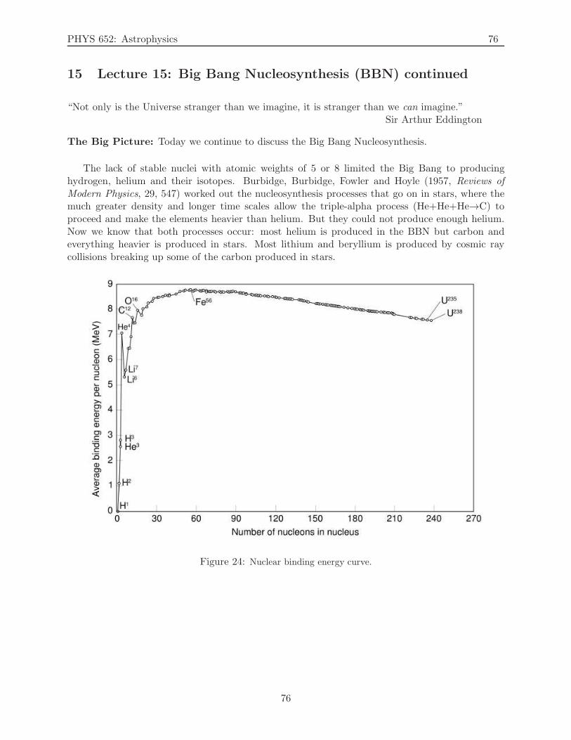
PHYS 652: Astrophysics 76
15 Lecture 15: Big Bang Nucleosynthesis (BBN) continued
“Not only is the Universe stranger than we imagine, it is stranger than we can imagine.”Sir Arthur Eddington
The Big Picture: Today we continue to discuss the Big Bang Nucleosynthesis.
The lack of stable nuclei with atomic weights of 5 or 8 limited the Big Bang to producinghydrogen, helium and their isotopes. Burbidge, Burbidge, Fowler and Hoyle (1957, Reviews ofModern Physics, 29, 547) worked out the nucleosynthesis processes that go on in stars, where themuch greater density and longer time scales allow the triple-alpha process (He+He+He→C) toproceed and make the elements heavier than helium. But they could not produce enough helium.Now we know that both processes occur: most helium is produced in the BBN but carbon andeverything heavier is produced in stars. Most lithium and beryllium is produced by cosmic raycollisions breaking up some of the carbon produced in stars.
Figure 24: Nuclear binding energy curve.
76
PHYS 652: Astrophysics 77
Neutron Abundance
Let us now compute the neutron-proton ratio. Neutrons and protons can be converted intoeach other via weak interaction:
p+ e− ↔ n+ νe
p+ νe ↔ n+ e+
n ↔ p+ e− + ν. (294)
When mp,mn ≫ T and the nucleons are in a non-relativistic regime (E = m+ p2/2m), we usethe appropriate portion of eq. (276):
n(0)p
n(0)n
=gp
(
mpT2π
)3/2e−mp/T
gn(
mnT2π
)3/2e−mn/T
=
(
mp
mn
)3/2
e(mn−mp)/T ≈ eQ/T , (295)
where we have used mp/mn ≈ 1 and defined Q ≡ mn−mp = 1.293 MeV. The equation above statesthat at high temperatures T ≫ Q, there are as many neutrons as protons. As the temperaturedrops beneath 1 MeV, the neutron fraction goes down. If these weak interactions were efficientenough to maintain equilibrium, the proton-neutron ratio in eq. (295) would grow to infinity, whichmeans that the abundance of neutrons relative to protons would be negligible. However, this is notthe case (as clearly as we are here!).
To enable a clearer analysis of neutron-proton interaction, define a ratio of neutrons to totalnucleons:
Xn ≡ nnnn + np
. (296)
In equilibrium np → n(0)p , nn → n
(0)n , so
Xn → Xn,EQ ≡ n(0)n
n(0)n + n
(0)p
=1
1 + (n(0)p /n
(0)n )
. (297)
Let us now track the evolution of Xn in the weak reaction where neutron and proton convertinto each other and produce leptons [first two reactions in eq. (294)]. In terms of the Boltzmannequation and the format of reaction 1 + 2 → 3 + 4, 1 = neutron, 3 = proton, 2,4 = leptons in
complete equilibrium (nl = n(0)l ). The Boltzmann equation [eq. (280)] then reads:
a−3 d
dt
(
n1a3)
= n(0)1 n
(0)2 〈σv〉
[
n3n4
n(0)3 n
(0)4
− n1n2
n(0)1 n
(0)2
]
a−3 d
dt
(
nna3)
= n(0)n n
(0)l 〈σv〉
[
npnl
n(0)p n
(0)l
− nnnl
n(0)n n
(0)l
]
= n(0)l 〈σv〉
[
npn(0)n
n(0)p
− nn
]
.
(298)
From eq. (295), we have that n(0)n
n(0)p
= e−Q/T . Also, we define
λnp ≡ n(0)l 〈σv〉, (299)
77
PHYS 652: Astrophysics 78
as the rate of neutron-proton conversion, because it multiplies nn in the loss term. If we writenn = Xn(nn + np), then we can rewrite the left-hand side of the eq. (298) as
a−3 d
dt
(
nna3)
= a−3 d
dt
(
Xn(nn + np)a3)
= a−3
dXn
dt(nn + np)a
3 +Xnd
dt
[
(nn + np)a3]
=dXn
dt(nn + np), (300)
since, as we derived earlier, ρba3 = const., so nba
3 = (nn+np)a3 = const., and d
dt
[
(nn + np)a3]
= 0.The right-hand side of the eq. (298) is simplified after expressing
nn =Xn
1−Xnnp, (301)
to yield
dXn
dt(nn + np) = λnp
npe−Q/T − Xn
1−Xnnp
=np
1−Xnλnp
(1−Xn)e−Q/T −Xn
=nnXn
λnp
(1−Xn)e−Q/T −Xn
=nnnn
nn+np
λnp
(1−Xn)e−Q/T −Xn
=⇒ dXn
dt= λnp
(1−Xn)e−Q/T −Xn
. (302)
The equation above is a function of temperature T and the reaction rate λnp, which both dependon time. We further “massage” the Boltzmann equation for interaction of neutron-nucleon ratioabove by introducing the evolution variable
x ≡ QT, (303)
so the left-hand side of the eq. (302) becomes
dXn
dt=
dXn
dx
dx
dt=
dXn
dx
[
−QT
T 2
]
=dXn
dx
[
−xT
T
]
. (304)
But, since T ∝ a−1 [see eq. (259)], or T = ka−1,
T
T=
k ddta
−1
ka−1=
−aa−2
a−1= −aa−1 = − a
a≡ −H = −
√
8πGρ
3. (305)
Now we needs to estimate the energy density of the Universe ρ. The BBN takes place during theradiation-dominated era, so the energy density of the Universe ρ will be determined by the rela-tivistic particles. We saw earlier [eq. (205) where g = 2] that the contribution from the relativisticparticles is
ρ = g⋆π2
30T 4 ≡ π2
30T 4
[
∑
i=bosons
gi +7
8
∑
i=fermions
gi
]
, (306)
where g⋆ is an effective number of relativistic degrees of freedom, and where a factor 7/8 comes froma + in the denominator for FD distribution. g⋆ is a function of temperature, because reactionsconstantly reshuffle relative abundances of fermions and bosons. At the time of the BBN, thetemperature is on the order of 1 MeV, at which time the contributing relativistic particles were:
78
PHYS 652: Astrophysics 79
• photons: gγ = 2 (2 spin states);
• neutrinos: gν = 6 (6 flavors);
• electrons: ge− = 2 (2 spin states);
• positrons: ge+ = 2 (2 spin states);
with the total being
g⋆ = 2 +7
8(6 + 2 + 2) = 2 +
70
8= 2 + 8.75 = 10.75. (307)
We also have that the Hubble rate H(x) can be expressed in terms of H(x = 1):
H(x) =
√
8πGρ
3ρ = g⋆
π2
30T 4
=
√
8πGg⋆π2T 4
90x4= x−2
√
4π3GQ4
45
√10.75 T =
Qx
≡ x−2H(x = 1). (308)
We compute the Hubble rate at x = 1 to be
H(x = 1) =
√
4π3GQ4
45
√10.75 = 1.13 s−1. (309)
After substituting eqs. (304)-(305) and (308)-(309) into eq. (302), we obtain
dXn
dt=
dXn
dxxH = λnp
(1−Xn)e−x −Xn
dXn
dx=
λnpxH
(1−Xn)e−x −Xn
=λnp
xH(x = 1)x−2
(1−Xn)e−x −Xn
=⇒ dXn
dx=
xλnpH(x = 1)
(1−Xn)e−x −Xn
. (310)
The rate of neutron-proton conversion λnp is defined as
λnp = n(0)νe 〈σv〉, (311)
and can be computed from eq. (279) (Extra credit on Homework set #2: problem 3b — note atypo in definition of τn in the textbook: it should be τ−1
n ) to yield:
λnp =255
τnx5(
x2 + 6x+ 12)
, (312)
where τn = 886.7s is the neutron mean lifetime. From the equation above, we see that whenT ≈ Q, i.e. , when x ≈ 1, the conversion rate is 5.5s−1, which is somewhat larger than theexpansion rate H(x = 1) = 1.13s−1. As the temperature drops below 1 MeV, the rate rapidly fallsbelow the expansion rate, so conversions become rare. One can compute the temperature at whichthe expansion rate H and the neutron-proton conversion rate λnp are equal:
H(x) = λnp(x)
H(x = 1)x−2 =255
τnx5(
x2 + 6x+ 12)
H(x = 1) =255
τnx3(
x2 + 6x+ 12)
=⇒ x = 1.9 =⇒ T = Q/x = 1.293/1.9 MeV = 0.68 MeV. (313)
79
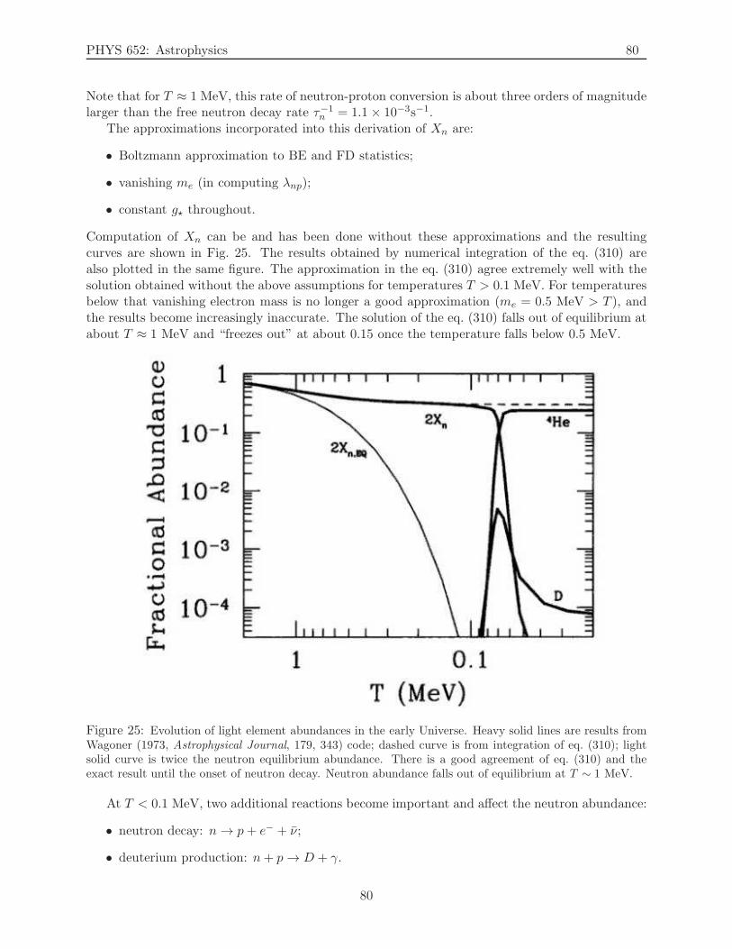
PHYS 652: Astrophysics 80
Note that for T ≈ 1 MeV, this rate of neutron-proton conversion is about three orders of magnitudelarger than the free neutron decay rate τ−1
n = 1.1× 10⁻³s−1.The approximations incorporated into this derivation of Xn are:
• Boltzmann approximation to BE and FD statistics;
• vanishing me (in computing λnp);
• constant g⋆ throughout.
Computation of Xn can be and has been done without these approximations and the resultingcurves are shown in Fig. 25. The results obtained by numerical integration of the eq. (310) arealso plotted in the same figure. The approximation in the eq. (310) agree extremely well with thesolution obtained without the above assumptions for temperatures T > 0.1 MeV. For temperaturesbelow that vanishing electron mass is no longer a good approximation (me = 0.5 MeV > T ), andthe results become increasingly inaccurate. The solution of the eq. (310) falls out of equilibrium atabout T ≈ 1 MeV and “freezes out” at about 0.15 once the temperature falls below 0.5 MeV.
Figure 25: Evolution of light element abundances in the early Universe. Heavy solid lines are results fromWagoner (1973, Astrophysical Journal, 179, 343) code; dashed curve is from integration of eq. (310); lightsolid curve is twice the neutron equilibrium abundance. There is a good agreement of eq. (310) and theexact result until the onset of neutron decay. Neutron abundance falls out of equilibrium at T ∼ 1 MeV.
At T < 0.1 MeV, two additional reactions become important and affect the neutron abundance:
• neutron decay: n → p+ e− + ν;
• deuterium production: n+ p → D + γ.
80
PHYS 652: Astrophysics 81
Neutron decay can be accounted for easily by multiplying the results of the eq. (310) by a factore−t/τn . These will become as important as the neutron-proton conversion considered in the eq. (310)when the rates become equal:
λnp = 1/τn =⇒ 1 =255
x5(
x2 + 6x+ 12)
=⇒ x = 7.92 =⇒ T =Qx
=1.293
7.92MeV = 0.16 MeV. (314)
By the time this happens, electrons and positrons have annihilated, so the effective number ofrelativistic degrees of freedom g⋆ in eq. (306) is found by
ρ = g⋆π2
30T 4 ≡ π2
30
[
T 4γ
∑
i=bosons
gi + T 4ν
7
8
∑
i=fermions
gi
]
=π2
30T 4γ
[
∑
i=bosons
gi +
(
TνTγ
)4 7
8
∑
i=fermions
gi
]
ρ =π2
30T 4γ
[
2 +
(
TνTγ
)4 7
86
]
=π2
30T 4γ
[
2 +
(
4
11
)4/3 21
4
]
=π2
30T 4γ [3.36]
=⇒ g⋆ = 3.36, (315)
where we have used the result from eq. (220): Tν/Tγ = (4/11)1/3 . The time-temperature relationis found after recognizing, again, that
H(x) =
√
8πGρ
3=
√
8πGg⋆π2T 4
90x4= x−2
√
4π3GQ4
45
√3.36
≡ x−2H(x = 1), (316)
where
H(x = 1) =
√
4π3GQ4
45
√3.36 = 0.632 s−1 or
H(x = 1)√3.36√
10.75, (317)
and
H(x) = x−2H(x = 1) =
(QT
)−2
H(x = 1) = − T
T
T 2 H(x = 1)
Q2= − T
T=⇒ H(x = 1)
Q2= − T
T 3
∫
H(x = 1)
Q dt = −∫
dT
T 3=⇒ H(x = 1)
Q2t =
1
2T−2
t =Q2
2H(x = 1)T−2 =⇒ t =
102Q2
2H(x = 1)
(
0.1MeV
T
)2
=102(1.293)2
2(0.632)
(
0.1MeV
T
)2
=⇒ t = 132 s
(
0.1MeV
T
)2
. (318)
The BBN— the start of production of deuterium and other light elements — starts around T ≈ 0.07MeV (as we will see shortly), by which time the decays have depleted neutron fraction by a factor
exp [−t/τc] = exp
[
−132 s(
0.1MeV0.07MeV
)2
886.7 s
]
= exp [−(132/886.7)(0.1/0.07)] = 0.74. (319)
So, the neutron abundance at the start of the BBN is 0.15× 0.74 = 0.11, or
Xn(Tnuc) = 0.11. (320)
81
PHYS 652: Astrophysics 82
16 Lecture 16: Light Element Abundances and Recombination
“We are just an advanced breed of monkeys on a minor planet of a very average star. But we canunderstand the Universe. That makes us something very special.”
Stephen Hawking
The Big Picture: Today we continue our exposition of the Big Bang Nucleosynthesis, by dis-cussing the abundances of light elements. We also discuss the recombination epoch of the Universe,when the first atoms began to form, and the Universe became opaque.
Review of Processes Leading Up to the Big Bang Nucleosynthesis
In order to understand which processes were taking place early in the Universe, we need tocompute the reaction rates and compare them to the rate of the expansion of the Universe H.Earlier, we have found that the expansion rate H and the neutron-proton conversion rates due toweak reactions λnp become equal at T ≈ 0.68 MeV [eq. (313)], and that the neutron decay rate τ−1
n
becomes equal to λnp at T ≈ 0.16 MeV [eq. (314)]. The remaining equality between the neutrondecay τ−1
n and the expansion H is easily found by solving:
τ−1n = H(x) = H(x = 1)x−2 =⇒ x =
√
H(x = 1)τn =√
(0.632s−1)(886.7s) = 23.64
=⇒ T = Q/x = 1.293/23.64 MeV
=⇒ T = 0.055 MeV. (321)
Temp. Description Reactions
> 1 MeV weak reactions on the right maintain the p+ e− ↔ n+ νeneutron-nucleon ratio in thermal equilibrium p+ ν ↔ n+ e+
≈ 0.68 MeV weak reaction rates λnp become slower than expansion H;neutron-nucleon rate eventually “freezes out” at ≈ 0.15
≈ 0.16 MeV neutron decay rate τ−1n is equal to weak reactions rate λnp
≈ 0.055 MeV neutron decay rate τ−1n is equal to the expansion H
< 0.1 MeV the only reaction that appreciably changes the number of n → p+ e− + νneutrons is neutron decay (τn = 886.7 s)
≈ 0.07 MeV deuterium nuclei production begins (BBN starts) p+ n → D+ γ
≈ 0.07 MeV helium nuclei production begins (with photon emission); D + n → 3H+ γthese reactions are slower because of the abundance 3H+ p → 4He + γof photons D + p → 3He + γ
3He + n → 4He + γ
≈ 0.07 MeV helium nuclei production begins (without photon emission) D +D → 3He + nD+D → 3H+ p3H+D → 4He + n3He + D → 4He + p
< 0.05 MeV helium nuclei production finishes D +D → 4He + γ(electrostatic repulsion of nuclei of D causes it to stop);most neutrons in the Universe end up in 4He nuclei
< 0.01 MeV deuterium nuclei abundance “freezes out” at ≈ 10−4 − 10−5
82
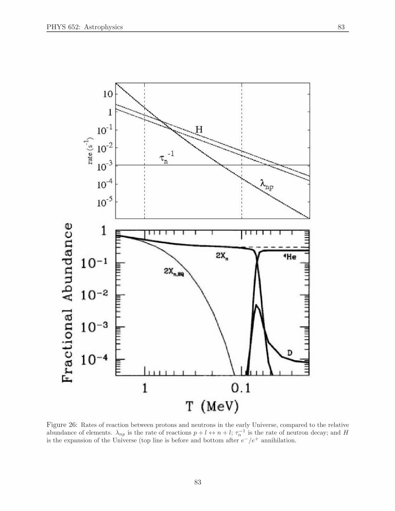
PHYS 652: Astrophysics 83
Figure 26: Rates of reaction between protons and neutrons in the early Universe, compared to the relativeabundance of elements. λnp is the rate of reactions p+ l ↔ n+ l; τ−1
n is the rate of neutron decay; and His the expansion of the Universe (top line is before and bottom after e−/e+ annihilation.
83
PHYS 652: Astrophysics 84
Light Element Abundances
Nuclei of light elements are produced as the temperature of the Universe drops below T = Tnuc.The first to be produced are the nucleons of the deuterium, via the reaction p+ n → D+ γ. If theUniverse stayed in equilibrium, all neutrons and protons would form deuterium, which means thatthe equilibrium deuterium abundance is on the order of baryon abundance. From the eq. (291), wecan see that the equilibrium deuterium-baryon ratio is of order unity when:
nDnb
≈ 6.77 ηb
(
Tnucmp
)3/2
eBD/Tnuc = 1
=⇒ ln(6.77 ηb) +3
2ln
(
Tnucmp
)
≈ − BD
Tnuc=⇒ Tnuc ≈ 0.07 MeV. (322)
The binding energy of helium is larger that of deuterium, which is why the factor eB/T in eq. (291)favors production of helium over deuterium. As can be seen from Fig. 26, production of heliumstarts almost immediately after deuterium starts forming. According to the Fig. 26, virtually allneutrons at T ≈ Tnuc are turned into nuclei of 4He. There are two neutrons and two protons in anucleus of 4He, which means that the final abundance of 4He is equal to about a half of neutronabundance at the onset of nucleosynthesis (T = Tnuc). If we define a mass fraction
X4 =4n4He
nb= 2Xn(Tnuc) = 0.22, (323)
where we have used eq. (320): Xn(Tnuc) = 0.11. This approximates to the exact solution well:
Yp = 0.2262 + 0.0135 ln(ηb/10−10). (324)
One important feature of this exact result is that the dependence of the helium-baryon ratio hasonly a logarithmic dependence on the baryon fraction ηb. This means that the abundance of heliumwill not be a good probe in determining the baryon energy density Ωb. The value of the abundanceof 4He hinges on the presence of a hot radiation field which prevents the formation of deuteriumbefore T = 0.1 MeV. Therefore, the fact that presently most of the matter is in the form ofhydrogen, i.e., not all the matter has transformed into 4He, is a strong argument for the existenceof a primeval cosmic background radiation.
Figure 26 shows that a portion of the deuterium remains unprocessed into helium, because thereaction which does this D + p → 3He + γ is not entirely efficient. It shows that the depletionof deuterium eventually “freezes out” at a level of order 10−5 − 10−4. The rate of this reactiondepends on the baryon density: if there are plenty of baryons to interact, the reactions will proceedeffectively; if the density of baryons is low, the depletion of deuterium will not be as effective.Therefore, abundance of deuterium is a powerful probe of the baryon density, as can be seen fromFig. 27. The measurements of primordial deuterium abundance show that the ratio of deuteriumto hydrogen is D/H = 3.0± 0.4 × 10⁻⁵, which corresponds to Ωbh
2 = 0.0205 ± 0.0018.
BBN Summarized
The BBN lasted for only a few minutes (during the period when the Universe was from 3 toabout 20 minutes old). After that, the temperature and density of the Universe fell below thatwhich is required for nuclear fusion. The brevity of BBN is important because it prevented elementsheavier than beryllium from forming while at the same time allowing unburned light elements, suchas deuterium, to exist.
84
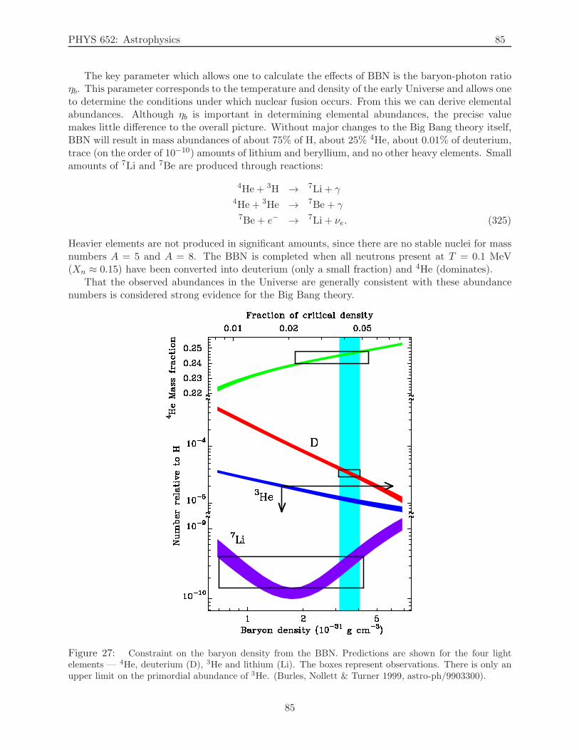
PHYS 652: Astrophysics 85
The key parameter which allows one to calculate the effects of BBN is the baryon-photon ratioηb. This parameter corresponds to the temperature and density of the early Universe and allows oneto determine the conditions under which nuclear fusion occurs. From this we can derive elementalabundances. Although ηb is important in determining elemental abundances, the precise valuemakes little difference to the overall picture. Without major changes to the Big Bang theory itself,BBN will result in mass abundances of about 75% of H, about 25% 4He, about 0.01% of deuterium,trace (on the order of 10−10) amounts of lithium and beryllium, and no other heavy elements. Smallamounts of 7Li and 7Be are produced through reactions:
4He + 3H → 7Li + γ4He + 3He → 7Be + γ7Be + e− → 7Li + νe. (325)
Heavier elements are not produced in significant amounts, since there are no stable nuclei for massnumbers A = 5 and A = 8. The BBN is completed when all neutrons present at T = 0.1 MeV(Xn ≈ 0.15) have been converted into deuterium (only a small fraction) and 4He (dominates).
That the observed abundances in the Universe are generally consistent with these abundancenumbers is considered strong evidence for the Big Bang theory.
Figure 27: Constraint on the baryon density from the BBN. Predictions are shown for the four lightelements — 4He, deuterium (D), 3He and lithium (Li). The boxes represent observations. There is only anupper limit on the primordial abundance of 3He. (Burles, Nollett & Turner 1999, astro-ph/9903300).
85
PHYS 652: Astrophysics 86
Recombination
When the temperature of the Universe drops to about T ≈ 1 eV, photons remain tightly coupledto electrons via Compton scattering and electrons to protons via Coulomb scattering. Even thoughthis temperature is significantly below the binding energy of the hydrogen electron of ǫ0 = 13.6eV, whenever a hydrogen atom is created, it is immediately ionized again by a high-energy photon.This delay is caused by the high photon-baryon ratio, and is similar to the delay we have seen inproduction of nuclei of light elements.
The Saha equation for the reaction which forms hydrogen atoms e− + p → H+ γ is given by
nenpnH
=n(0)e n
(0)p
n(0)H
. (326)
The equation above is simplified when we realize that the Universe is neutral in charge, whichmeans ne = np. We can now define a free electron fraction:
Xe ≡ne
ne + nH=
npnp + nH
, (327)
and rewrite the left-hand side of the eq. (326) in terms of Xe:
nenpnH
=nenp
(ne + nH)2(ne + nH)
2
nH= XeXp(ne + nH)
1
1−Xe=
X2e
1−Xe(ne + nH). (328)
The right-hand side of the eq. (326) is obtained from the eq. (276):
n(0)e n
(0)p
n(0)H
=ge(
meT2π
)3/2e−me/T gp
(
mpT2π
)3/2e−mp/T
gH
(
mHT2π
)3/2e−mH/T
mH ≈ mp
=gegpgH
(
meT
2π
)3/2
e−(me+mp−mH )/T =
(
meT
2π
)3/2
e−ǫ0/T , (329)
where we have recognized that ǫ0 = me +mp −mH . Saha equation then reads:
X2e
1−Xe=
1
ne + nH
(
meT
2π
)3/2
e−ǫ0/T , (330)
If we neglect a relatively small number of helium atoms, and recall that ne = np, then the denom-inator in the equation above is ne + nH = np + nH ≈ nb. A good approximation of the baryonnumber density nb is found by combining eqs. (276) and (286):
nb ≡ ηbnγ =
[
5.5 × 10⁻¹⁰
(
Ωbh2
0.02
)][
2T 3
π2
]
≈ 10−10T 3. (331)
This means that when the temperature of the Universe is of the order of ǫ0 = 13.6eV, the right-handside of the eq. (330) is
RHS(T = ǫ0) = 1010ǫ−30
(meǫ02π
)3/2e−1 = 1010
(
me
ǫ0
)3/2 1
e(2π)3/2
= 1010(
5.1 × 10⁵ eV
13.6 eV
)3/2
2.34 × 10⁻² ≈ 1.7 × 10¹⁵. (332)
86
PHYS 652: Astrophysics 87
Since Xe is, by definition 0 ≤ Xe ≤ 1, the only way that the equality in eq. (330) can hold is if Xe
is very close to 1. From the definition of Xe, this means that nH = 0, i.e., all hydrogen is ionized.When the temperature falls markedly below ǫ0, a significant amount of recombination takes place.As Xe drops, the rate of recombination also drops, so the equilibrium can no longer be maintained.In order to track the number density of free electrons accurately, we, again, use the Boltzmannequation for annihilation, just as we did for the neutron-nucleon ratio.
For the reaction e− + p → H+ γ (1=e, 2=p, 3=H, 4=γ) The Boltzmann equation is given by:
a−3 d
dt
(
nea3)
= n(0)e n(0)
p 〈σv〉[
nHnγ
n(0)H n
(0)γ
− nenp
n(0)e n
(0)p
]
= 〈σv〉[
n(0)e n
(0)p
n(0)H
nH − n2e
]
a−3 d
dt
(
Xenba3)
= 〈σv〉[
(
meT
2π
)3/2
e−ǫ0/TnH −X2en
2b
]
Xe =nenb
a−3nba3 dXe
dt= nb〈σv〉
[
(1−Xe)
(
meT
2π
)3/2
e−ǫ0/T −X2enb
]
nH = (1−Xe)nb
=⇒ dXe
dt= 〈σv〉
[
(1−Xe)
(
meT
2π
)3/2
e−ǫ0/T −X2enb
]
. (333)
After defining the recombination rate α(2) and the ionization rate β:
α(2) ≡ 〈σv〉,
β ≡ 〈σv〉(
meT
2π
)3/2
e−ǫ0/T = α(2)
(
meT
2π
)3/2
e−ǫ0/T , (334)
the differential equation for Xe above can be rewritten as
dXe
dt=[
(1−Xe) β − α(2)X2enb
]
. (335)
The superscript (2) in the recombination rate α(2) denotes the n = 2 state of the electron. Theground state (n = 1) leads to production of an ionizing photon, which immediately ionizes anotherneutral atom, thus leading to zero net effect — no neutral atoms are formed this way. The onlyway for the recombination to proceed is by capturing an electron in one of the excited states ofhydrogen. This rate is well-approximated by
α(2) = 9.78α2
m2e
(ǫeT
)1/2ln(ǫ0T
)
. (336)
The Saha approximation in eq. (330) is a good approximation to the electron-baryon ration Xe
until it falls out of equilibrium. It even correctly predicts the onset of recombination. However,as we have seen earlier, Saha equation is not valid when equilibrium is not preserved. The correctdescription of the evolution of Xe in the presence of reactions leading to the formation of neutralatoms is accurately described by the full Boltzmann equation given in eq. (335).
We present exact solutions and compare them to Saha equilibrium solutions as we continue ourdiscussion next time.
87
PHYS 652: Astrophysics 88
17 Lecture 17: Recombination and Dark Matter Production
“New ideas pass through three periods:
• It can’t be done.
• It probably can be done, but it’s not worth doing.
• I knew it was a good idea all along!”
Arthur C. Clarke
The Big Picture: Today we continue discussing the recombination epoch in the early Universe.We also extend the Boltzmann formalism to the production of dark matter particles.
Recombination (continued)
Just as the neutron-nucleon ratio Xn is important to the abundance of light elements, the abun-dance of free electrons Xe is of great significance to the observational cosmology. Recombination,which takes place around z ≈ 1000 directly leads to decoupling of photons from matter. Decouplingmeans that the photons stopped scattering off electrons, which become bound to neutral atomsduring this epoch. The mean-free paths of photons become on the order of the size of the Uni-verse, meaning that the Universe has become opaque. The resulting CMB radiation represents a“snapshot” of the Universe at the time of the “last scatter”.
Roughly speaking, decoupling occurs when the rate of Compton scattering of photons off elec-trons becomes smaller than the expansion rate of the Universe. The scattering rate is
neσT = XenbσT , (337)
where σT = 0.665×10⁻²⁴cm2 is the Thomson cross-section, and we continue to ignore contributionof 4He, by approximating ne + nH ≈ nb. The ratio of the baryon density to the critical density is
Ωb ≡ ρbρcr0
=mpnbρcr0
ρcr0 = 1.87 × 10⁻²⁹h2g cm−3
Ωb = Ωb0a−3
=⇒ nb =ρcr0mp
Ωb0a−3 =
1.87 × 10⁻²⁹ g cm−3
1.67 × 10⁻²⁴ gh2Ωb0a
−3
=⇒ nb = 1.12 × 10⁻⁵ h2Ωb0a−3 cm−3, (338)
so that the eq. (337) the becomes
neσT = 7.448 × 10⁻³⁰ cm−1 XeΩb0h2a−3. (339)
From eq. (73), we have
H0 =h
0.98 × 10¹⁰ years
(
1 year
3600 × 24× 365.25 s
)
= 0.323 × 10⁻¹⁷ s−1h,
h = 3.09 × 10¹⁷s H0, (340)
so that the eq. (339) can be rewritten as
neσT = 7.448 × 10⁻³⁰ cm−1 XeΩb0ha−3(
3.09× 10¹⁷s)
H0
= 2.3 × 10⁻¹² s cm−1 XeΩb0ha−3H0. (341)
88
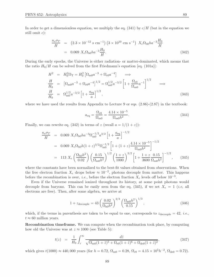
PHYS 652: Astrophysics 89
In order to get a dimensionless equation, we multiply the eq. (341) by c/H (but in the equation westill omit c):
neσTH
=(
2.3× 10⁻¹² s cm−1) (
3× 1010 cm s−1)
XeΩb0ha−3H0
H
= 0.069 XeΩb0ha−3H0
H. (342)
During the early epochs, the Universe is either radiation- or matter-dominated, which means thatthe ratio H0/H can be solved from the first Friedmann’s equation [eq. (101a)]:
H2 = H20ΩT = H2
0
[
Ωm0a−3 +Ωr0a
−4]
=⇒H
H0=
[
Ωm0a−3 +Ωr0a
−4]1/2
= Ω1/2m0 a
−3/2
[
1 +Ωr0
Ωm0a−1
]1/2
=⇒
H
H0= Ω
1/2m0 a
−3/2[
1 +aeqa
]1/2, (343)
where we have used the results from Appendix to Lecture 9 or eqs. (2.86)-(2.87) in the textbook:
aeq =Ωr0
Ωm0=
4.14 × 10⁻⁵
Ωm0h2. (344)
Finally, we can rewrite eq. (342) in terms of z (recall a = 1/(1 + z)):
neσTH
= 0.069 XeΩb0ha−3Ω
−1/2m0 a3/2
[
1 +aeqa
]−1/2
= 0.069 XeΩb0h(1 + z)3/2Ω−1/2m0
[
1 + (1 + z)4.14 × 10⁻⁵
Ωm0h2
]−1/2
= 113 Xe
(
Ωb0h2
0.02
)(
0.15
Ωm0h2
)1/2(1 + z
1000
)3/2 [
1 +1 + z
3600
0.15
Ωm0h2
]−1/2
, (345)
where the constants have been normalized to the best-fit values obtained from observations. Whenthe free electron fraction Xe drops below ≈ 10−2, photons decouple from matter. This happensbefore the recombination is over, i.e., before the electron fraction Xe levels off below 10−3.
Even if the Universe remained ionized throughout its history, at some point photons woulddecouple from baryons. This can be easily seen from the eq. (345), if we set Xe = 1 (i.e, allelectrons are free). Then, after some algebra, we arrive at
1 + zdecouple = 43
(
0.02
Ωb0h2
)2/3(Ωm0h2
0.15
)1/3
, (346)
which, if the terms in parenthesis are taken to be equal to one, corresponds to zdecouple = 42, i.e.,t ≈ 60 million years.
Recombination timeframe. We can compute when the recombination took place, by computinghow old the Universe was at z ≈ 1000 (see Table 5):
t(z) =1
H0
∫ ∞
z
dz√
Ωm0(1 + z)5 +Ωr0(1 + z)6 +Ωde0(1 + z)2, (347)
which gives t(1000) ≈ 440, 000 years (for h = 0.72, Ωm0 = 0.28, Ωr0 = 4.15× 10⁵h−2, Ωde0 = 0.72).
89
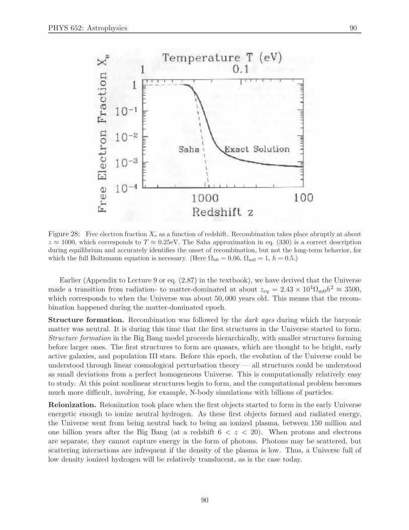
PHYS 652: Astrophysics 90
Figure 28: Free electron fraction Xe as a function of redshift. Recombination takes place abruptly at aboutz ≈ 1000, which corresponds to T ≈ 0.25eV. The Saha approximation in eq. (330) is a correct descriptionduring equilibrium and accurately identifies the onset of recombination, but not the long-term behavior, forwhich the full Boltzmann equation is necessary. (Here Ωb0 = 0.06, Ωm0 = 1, h = 0.5.)
Earlier (Appendix to Lecture 9 or eq. (2.87) in the textbook), we have derived that the Universemade a transition from radiation- to matter-dominated at about zeq = 2.43 × 10⁴Ωm0h
2 ≈ 3500,which corresponds to when the Universe was about 50, 000 years old. This means that the recom-bination happened during the matter-dominated epoch.
Structure formation. Recombination was followed by the dark ages during which the baryonicmatter was neutral. It is during this time that the first structures in the Universe started to form.Structure formation in the Big Bang model proceeds hierarchically, with smaller structures formingbefore larger ones. The first structures to form are quasars, which are thought to be bright, earlyactive galaxies, and population III stars. Before this epoch, the evolution of the Universe could beunderstood through linear cosmological perturbation theory — all structures could be understoodas small deviations from a perfect homogeneous Universe. This is computationally relatively easyto study. At this point nonlinear structures begin to form, and the computational problem becomesmuch more difficult, involving, for example, N-body simulations with billions of particles.
Reionization. Reionization took place when the first objects started to form in the early Universeenergetic enough to ionize neutral hydrogen. As these first objects formed and radiated energy,the Universe went from being neutral back to being an ionized plasma, between 150 million andone billion years after the Big Bang (at a redshift 6 < z < 20). When protons and electronsare separate, they cannot capture energy in the form of photons. Photons may be scattered, butscattering interactions are infrequent if the density of the plasma is low. Thus, a Universe full oflow density ionized hydrogen will be relatively translucent, as is the case today.
90
PHYS 652: Astrophysics 91
Dark Matter
Earlier, in Lectures 10 and 11, we discussed the evidence for nonbaryonic matter in the Universe,and came to the general conclusion that the total contribution of the such a matter to the energydensity is Ωdm ≈ 0.3. We also established WIMPs as the leading candidates for the nonbaryonicdark matter. Even though we do not know yet what these particles are, we do know that ifsuch particles exist, they were at some point in equilibrium with the rest of the cosmic plasmaat high temperatures of the early Universe. At some point, they experienced “freeze-out” as thetemperature of the Universe dropped below the WIMP’s mass. Had it not been for falling out ofthe equilibrium (“freeze-out”), the abundance of the dark matter particles would decay as e−m/T ,which would lead to their extinction. However, they do freeze out at some point, which is why weuse the Boltzmann equation (instead of its equilibrium version, the Saha equation) to determinewhen they froze-out and quantify their relic abundance. The idea is to use the conclusions fromobservations and the earlier epochs of the Big Bang (the BBN), such as Ωdm ≈ 0.3, to constrainthe properties of the unknown WIMPs: their mass and cross-section. Putting such constraints onthe WIMPs would be useful in the experimental attempts at their direct detection.
We now consider a generic scenario, in which two heavy WIMPs (denoted as X) annihilateand produce two light (essentially massless) particles (l). The light particles are assumed to be
in complete equilibrium to the cosmic plasma, which means nl = n(0)l . This means that in the
reaction X +X → l + l (1=X, 2=X, 3=l, 4=l), there is only one unknown nX , the abundance ofthe WIMPs. Again, we use the Boltzmann equation [eq. (280)]:
a−3 d
dt
(
nXa3)
= n(0)X n
(0)X 〈σv〉
[
nlnl
n(0)l n
(0)l
− nXnX
n(0)X n
(0)X
]
=
a−3 d
dt
(
nXa3)
= 〈σv〉[
(
n(0)X
)2− n2
X
]
. (348)
As we did before, we continue to “massage” the Boltzmann equation into something mathematicallymore elucidating. After recalling that the temperature scales as T ∼ a−1, we can rewrite the RHSof the eq. (348) above as:
a−3 d
dt
(
nXa3)
= a−3 d
dt
(nXT 3
T 3a3)
= a−3T 3a3d
dt
(nXT 3
)
= T 3 d
dt
(nXT 3
)
. (349)
After defining the quantity Y as
Y ≡ nXT 3
, (350)
we can rewrite the eq. (348) above as
T 3dY
dt= 〈σv〉T 6
(
n(0)X
T 3
)2
−(nXT 3
)2
,
=⇒ dY
dt= 〈σv〉T 3
[
Y 2EQ − Y 2
]
, (351)
where YEQ ≡ n(0)X /T 3. It is, again, beneficial to introduce a new time variable:
x ≡ mX
T, (352)
where mX is the mass of the WIMP. Again, very high temperatures correspond to x ≪ 1, whichis when the reactions proceed so rapidly to maintain equilibrium Y ≈ YEQ. Since the WIMPs
91
PHYS 652: Astrophysics 92
are relativistic at that time, their equilibrium abundance is given by the m ≪ T portion of theeq. (276), so
Y ≈ YEQ =n(0)X
T 3=
gXT3
π2
T 3=
gXπ2
∼ 1. (353)
For x ≫ 1, the exponent e−x dominates and suppresses the equilibrium abundance YEQ. Eventually,the WIMPs become so rare due to this suppression that they no longer can find each other fastenough to maintain the equilibrium abundance. This is when the freeze-out begins.
We rewrite the Boltzmann equation in terms of the new integration variable x:
dY
dt=
dY
dx
dx
dt=
dY
dx
[
− T
Tx
]
= −dY
dxx
[−ka−2a
ka−1
]
=dY
dxx
[
a
a
]
=dY
dxxH
=dY
dxxH(x = 1)
x2=
dY
dx
H(x = 1)
x= 〈σv〉T 3
[
Y 2EQ − Y 2
]
=⇒ dY
dx=
x
H(x = 1)〈σv〉T 3
[
Y 2EQ − Y 2
]
=m3X〈σv〉
H(x = 1)
T 3
m3X
x[
Y 2EQ − Y 2
]
=⇒ dY
dx= − λ
x2[
Y 2 − Y 2EQ
]
, (354)
where the ratio of annihilation rate to the expansion rate is given by
λ ≡ m3X〈σv〉
H(x = 1). (355)
In most theories, λ is a constant. Some theories, however, have a temperature-dependent thermally-averaged cross-section, which leads to a variable λ. This changes the quantitative results slightly,while the qualitative solutions remain the same.
92
PHYS 652: Astrophysics 93
18 Lecture 18: Dark Matter Particle Production
“The simple is the seal of the true.”Subrahmanyan Chandrasekhar (on GR)
The Big Picture: Today we finish the discussion of dark matter particle production. Eventhough we do not know the mass of the particles, the Boltzmann equation can be used to derivethe relationship between the mass of particles and its present-day abundance.
Dark Matter Particle Production (continued)
The eq. (354) is not analytically tractable, so its solution requires numerical evaluation. How-ever, we can, again, get a good quantitative feel about its behavior through simple analysis of theorders of magnitude of the terms, as we have done earlier. When x ∼ 1, the left-hand side of the
eq. (354) is on the order of Y , while the right hand side is on the order of λ(
Y 2 − Y 2EQ
)
. Since
λ is quite large, the equality is maintained only with Y ≈ YEQ. Later, as temperature T drops, xincreases, and the equilibrium YEQ is no longer a good approximation to Y . After the freeze-out, Yis much larger than YEQ, as particles are not able to annihilate fast enough to maintain equilibrium.Therefore, at later times
dY
dx≃ −λY 2
x2, for x ≫ 1. (356)
This equation can be integrated analytically from the epoch of freeze-out x = xf , Y = Yf untilvery late times x = ∞, Y = Y∞ to obtain
∫ Y∞
Yf
dY
Y 2≃ −
∫ ∞
xf
λ dx
x2=⇒ − 1
Y
∣
∣
∣
∣
Y∞
Yf
=λ
x
∣
∣
∣
∣
∞
xf
=⇒ − 1
Y∞+
1
Yf≃ − λ
xf
=⇒ 1
Y∞− 1
Yf=
λ
xf. (357)
Generally, Y at freeze-out Yf is much larger than Y∞, so 1/Y∞ ≫ 1/Yf , and the term 1/Yf can beneglected. Then a simple analytic approximation for Y∞ is
Y∞ ≃ xfλ. (358)
This approximation still depends on the freeze-out temperature xf which is yet to be determined.Typically, xf ∼ 10.
Figure 29 shows that the numerical solution to eq. (354) for two different values of λ. Theequilibrium approximation is valid to about m/T ≈ 10, after which the Boltzmann non-equilibriumsolution levels off. The rough approximation of Y∞ ≈ 10/λ is a decent approximation for therelic abundance. The particles with the larger cross-sections (and consequently, by definition,larger λ) freeze-out later, because the bigger the cross-section, the longer they will continue tointeract. Furthermore, this prolonged annihilation results in a lower relic abundance. The inset inFig. (29) shows that the distinction between BE, FD and Boltzmann statistics is only important fortemperatures above the particle’s mass. Since the freeze-out happens at temperatures significantlybelow the particle’s mass (recall the delay in freezing-out), the use of Boltzmann statistics isjustified. At the freeze-out, the dark matter particle density scales as ρX ∝ a−3. This means that
93
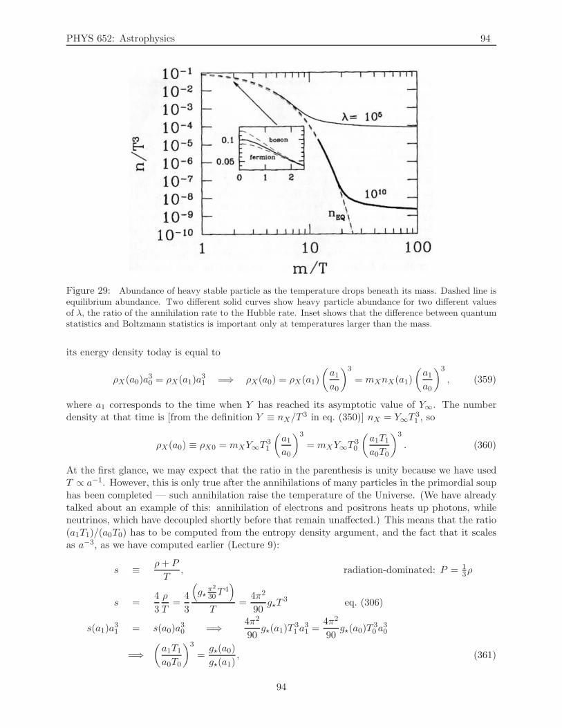
PHYS 652: Astrophysics 94
Figure 29: Abundance of heavy stable particle as the temperature drops beneath its mass. Dashed line isequilibrium abundance. Two different solid curves show heavy particle abundance for two different valuesof λ, the ratio of the annihilation rate to the Hubble rate. Inset shows that the difference between quantumstatistics and Boltzmann statistics is important only at temperatures larger than the mass.
its energy density today is equal to
ρX(a0)a30 = ρX(a1)a
31 =⇒ ρX(a0) = ρX(a1)
(
a1a0
)3
= mXnX(a1)
(
a1a0
)3
, (359)
where a1 corresponds to the time when Y has reached its asymptotic value of Y∞. The numberdensity at that time is [from the definition Y ≡ nX/T
3 in eq. (350)] nX = Y∞T 31 , so
ρX(a0) ≡ ρX0 = mXY∞T 31
(
a1a0
)3
= mXY∞T 30
(
a1T1
a0T0
)3
. (360)
At the first glance, we may expect that the ratio in the parenthesis is unity because we have usedT ∝ a−1. However, this is only true after the annihilations of many particles in the primordial souphas been completed — such annihilation raise the temperature of the Universe. (We have alreadytalked about an example of this: annihilation of electrons and positrons heats up photons, whileneutrinos, which have decoupled shortly before that remain unaffected.) This means that the ratio(a1T1)/(a0T0) has to be computed from the entropy density argument, and the fact that it scalesas a−3, as we have computed earlier (Lecture 9):
s ≡ ρ+ P
T, radiation-dominated: P = 1
3ρ
s =4
3
ρ
T=
4
3
(
g⋆π2
30T4)
T=
4π2
90g⋆T
3 eq. (306)
s(a1)a31 = s(a0)a
30 =⇒ 4π2
90g⋆(a1)T
31 a
31 =
4π2
90g⋆(a0)T
30 a
30
=⇒(
a1T1
a0T0
)3
=g⋆(a0)
g⋆(a1), (361)
94
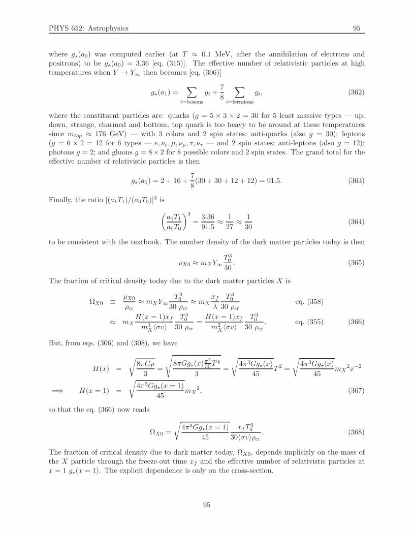
PHYS 652: Astrophysics 95
where g⋆(a0) was computed earlier (at T ≈ 0.1 MeV, after the annihilation of electrons andpositrons) to be g⋆(a0) = 3.36 [eq. (315)]. The effective number of relativistic particles at hightemperatures when Y → Y∞ then becomes [eq. (306)]
g⋆(a1) =∑
i=bosons
gi +7
8
∑
i=fermions
gi, (362)
where the constituent particles are: quarks (g = 5 × 3 × 2 = 30 for 5 least massive types — up,down, strange, charmed and bottom; top quark is too heavy to be around at these temperaturessince mtop ≈ 176 GeV) — with 3 colors and 2 spin states; anti-quarks (also g = 30); leptons(g = 6 × 2 = 12 for 6 types — e, νe, µ, νµ, τ, ντ — and 2 spin states; anti-leptons (also g = 12);photons g = 2; and gluons g = 8× 2 for 8 possible colors and 2 spin states. The grand total for theeffective number of relativistic particles is then
g⋆(a1) = 2 + 16 +7
8(30 + 30 + 12 + 12) = 91.5. (363)
Finally, the ratio [(a1T1)/(a0T0)]3 is
(
a1T1
a0T0
)3
=3.36
91.5≈ 1
27≈ 1
30(364)
to be consistent with the textbook. The number density of the dark matter particles today is then
ρX0 ≈ mXY∞T 30
30. (365)
The fraction of critical density today due to the dark matter particles X is
ΩX0 ≡ ρX0
ρcr≈ mXY∞
T 30
30 ρcr≈ mX
xfλ
T 30
30 ρcreq. (358)
≈ mXH(x = 1)xfm3X〈σv〉
T 30
30 ρcr=
H(x = 1)xfm2X〈σv〉
T 30
30 ρcr. eq. (355) (366)
But, from eqs. (306) and (308), we have
H(x) =
√
8πGρ
3=
√
8πGg⋆(x)π2
30T4
3=
√
4π3Gg⋆(x)
45T 2 =
√
4π3Gg⋆(x)
45mX
2x−2
=⇒ H(x = 1) =
√
4π3Gg⋆(x = 1)
45mX
2, (367)
so that the eq. (366) now reads
ΩX0 =
√
4π3Gg⋆(x = 1)
45
xfT30
30〈σv〉ρcr. (368)
The fraction of critical density due to dark matter today, ΩX0, depends implicitly on the mass ofthe X particle through the freeze-out time xf and the effective number of relativistic particles atx = 1 g⋆(x = 1). The explicit dependence is only on the cross-section.
95
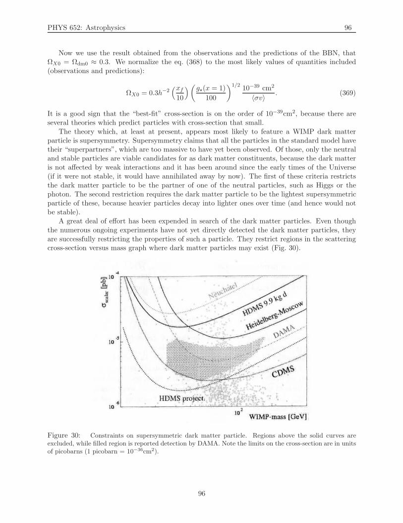
PHYS 652: Astrophysics 96
Now we use the result obtained from the observations and the predictions of the BBN, thatΩX0 = Ωdm0 ≈ 0.3. We normalize the eq. (368) to the most likely values of quantities included(observations and predictions):
ΩX0 = 0.3h−2(xf10
)
(
g⋆(x = 1)
100
)1/2 10−39 cm2
〈σv〉 . (369)
It is a good sign that the “best-fit” cross-section is on the order of 10−39cm2, because there areseveral theories which predict particles with cross-section that small.
The theory which, at least at present, appears most likely to feature a WIMP dark matterparticle is supersymmetry. Supersymmetry claims that all the particles in the standard model havetheir “superpartners”, which are too massive to have yet been observed. Of those, only the neutraland stable particles are viable candidates for as dark matter constituents, because the dark matteris not affected by weak interactions and it has been around since the early times of the Universe(if it were not stable, it would have annihilated away by now). The first of these criteria restrictsthe dark matter particle to be the partner of one of the neutral particles, such as Higgs or thephoton. The second restriction requires the dark matter particle to be the lightest supersymmetricparticle of these, because heavier particles decay into lighter ones over time (and hence would notbe stable).
A great deal of effort has been expended in search of the dark matter particles. Even thoughthe numerous ongoing experiments have not yet directly detected the dark matter particles, theyare successfully restricting the properties of such a particle. They restrict regions in the scatteringcross-section versus mass graph where dark matter particles may exist (Fig. 30).
Figure 30: Constraints on supersymmetric dark matter particle. Regions above the solid curves areexcluded, while filled region is reported detection by DAMA. Note the limits on the cross-section are in unitsof picobarns (1 picobarn = 10−36cm2).
96
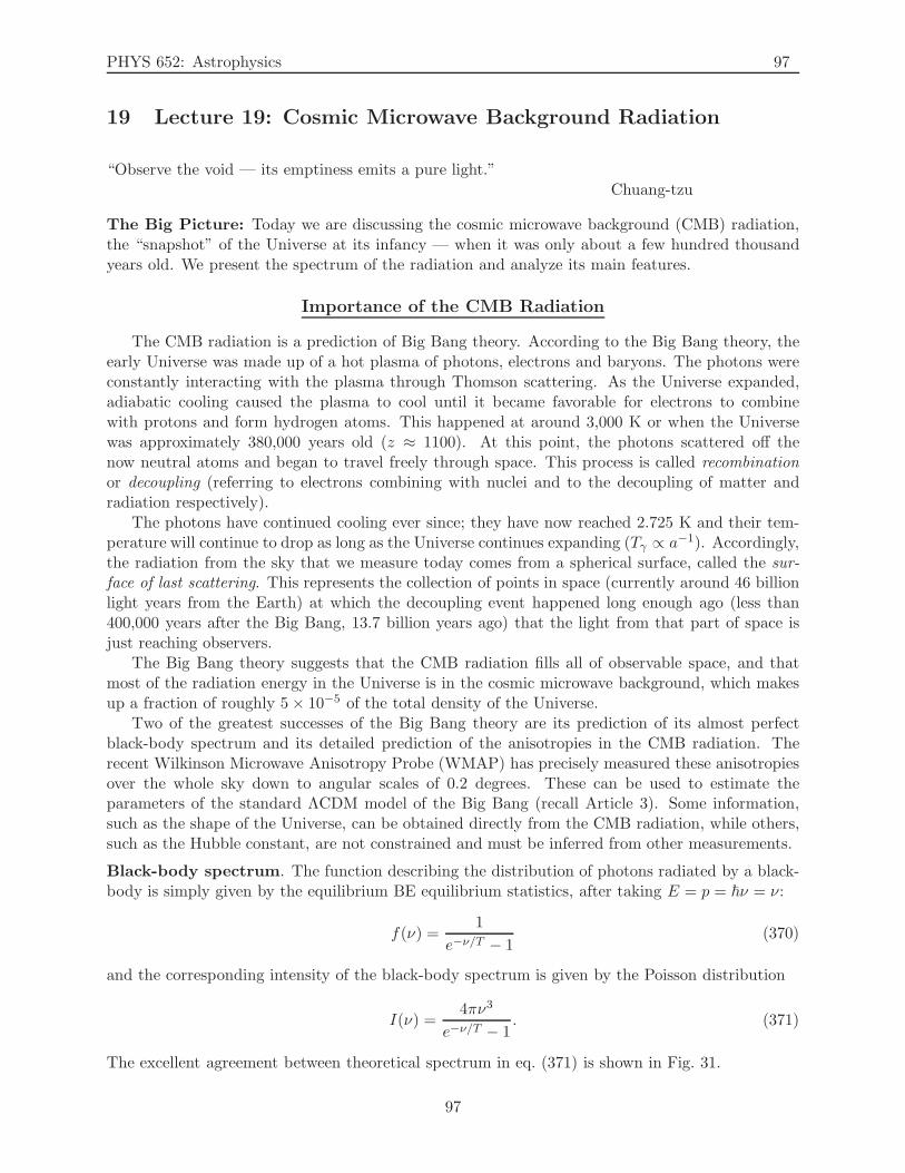
PHYS 652: Astrophysics 97
19 Lecture 19: Cosmic Microwave Background Radiation
“Observe the void — its emptiness emits a pure light.”Chuang-tzu
The Big Picture: Today we are discussing the cosmic microwave background (CMB) radiation,the “snapshot” of the Universe at its infancy — when it was only about a few hundred thousandyears old. We present the spectrum of the radiation and analyze its main features.
Importance of the CMB Radiation
The CMB radiation is a prediction of Big Bang theory. According to the Big Bang theory, theearly Universe was made up of a hot plasma of photons, electrons and baryons. The photons wereconstantly interacting with the plasma through Thomson scattering. As the Universe expanded,adiabatic cooling caused the plasma to cool until it became favorable for electrons to combinewith protons and form hydrogen atoms. This happened at around 3,000 K or when the Universewas approximately 380,000 years old (z ≈ 1100). At this point, the photons scattered off thenow neutral atoms and began to travel freely through space. This process is called recombinationor decoupling (referring to electrons combining with nuclei and to the decoupling of matter andradiation respectively).
The photons have continued cooling ever since; they have now reached 2.725 K and their tem-perature will continue to drop as long as the Universe continues expanding (Tγ ∝ a−1). Accordingly,the radiation from the sky that we measure today comes from a spherical surface, called the sur-face of last scattering. This represents the collection of points in space (currently around 46 billionlight years from the Earth) at which the decoupling event happened long enough ago (less than400,000 years after the Big Bang, 13.7 billion years ago) that the light from that part of space isjust reaching observers.
The Big Bang theory suggests that the CMB radiation fills all of observable space, and thatmost of the radiation energy in the Universe is in the cosmic microwave background, which makesup a fraction of roughly 5× 10⁻⁵ of the total density of the Universe.
Two of the greatest successes of the Big Bang theory are its prediction of its almost perfectblack-body spectrum and its detailed prediction of the anisotropies in the CMB radiation. Therecent Wilkinson Microwave Anisotropy Probe (WMAP) has precisely measured these anisotropiesover the whole sky down to angular scales of 0.2 degrees. These can be used to estimate theparameters of the standard ΛCDM model of the Big Bang (recall Article 3). Some information,such as the shape of the Universe, can be obtained directly from the CMB radiation, while others,such as the Hubble constant, are not constrained and must be inferred from other measurements.
Black-body spectrum. The function describing the distribution of photons radiated by a black-body is simply given by the equilibrium BE equilibrium statistics, after taking E = p = ~ν = ν:
f(ν) =1
e−ν/T − 1(370)
and the corresponding intensity of the black-body spectrum is given by the Poisson distribution
I(ν) =4πν3
e−ν/T − 1. (371)
The excellent agreement between theoretical spectrum in eq. (371) is shown in Fig. 31.
97
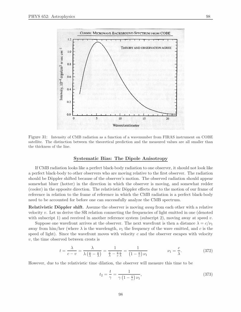
PHYS 652: Astrophysics 98
Figure 31: Intensity of CMB radiation as a function of a wavenumber from FIRAS instrument on COBEsatellite. The distinction between the theoretical prediction and the measured values are all smaller thanthe thickness of the line.
Systematic Bias: The Dipole Anisotropy
If CMB radiation looks like a perfect black-body radiation to one observer, it should not look likea perfect black-body to other observers who are moving relative to the first observer. The radiationshould be Doppler shifted because of the observer’s motion. The observed radiation should appearsomewhat bluer (hotter) in the direction in which the observer is moving, and somewhat redder(cooler) in the opposite direction. The relativistic Doppler effects due to the motion of our frame ofreference in relation to the frame of reference in which the CMB radiation is a perfect black-bodyneed to be accounted for before one can successfully analyze the CMB spectrum.
Relativistic Doppler shift. Assume the observer is moving away from each other with a relativevelocity v. Let us derive the SR relation connecting the frequencies of light emitted in one (denotedwith subscript 1) and received in another reference system (subscript 2), moving away at speed v.
Suppose one wavefront arrives at the observer. The next wavefront is then a distance λ = c/ν1away from him/her (where λ is the wavelength, ν1 the frequency of the wave emitted, and c is thespeed of light). Since the wavefront moves with velocity c and the observer escapes with velocityv, the time observed between crests is
t =λ
c− v=
λ
λ(
cλ − v
λ
) =1
cλ − v
ccλ
=1
(
1− vc
)
ν1ν1 =
c
λ. (372)
However, due to the relativistic time dilation, the observer will measure this time to be
t2 =t
γ=
1
γ(
1− vc
)
ν1, (373)
98
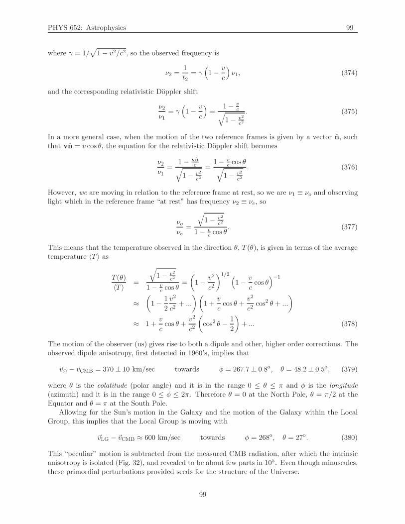
PHYS 652: Astrophysics 99
where γ = 1/√
1− v2/c2, so the observed frequency is
ν2 =1
t2= γ
(
1− v
c
)
ν1, (374)
and the corresponding relativistic Doppler shift
ν2ν1
= γ(
1− v
c
)
=1− v
c√
1− v2
c2
. (375)
In a more general case, when the motion of the two reference frames is given by a vector n, suchthat vn = v cos θ, the equation for the relativistic Doppler shift becomes
ν2ν1
=1− vn
c√
1− v2
c2
=1− v
c cos θ√
1− v2
c2
. (376)
However, we are moving in relation to the reference frame at rest, so we are ν1 ≡ νo and observinglight which in the reference frame “at rest” has frequency ν2 ≡ νe, so
νoνe
=
√
1− v2
c2
1− vc cos θ
. (377)
This means that the temperature observed in the direction θ, T (θ), is given in terms of the averagetemperature 〈T 〉 as
T (θ)
〈T 〉 =
√
1− v2
c2
1− vc cos θ
=
(
1− v2
c2
)1/2(
1− v
ccos θ
)−1
≈(
1− 1
2
v2
c2+ ...
)(
1 +v
ccos θ +
v2
c2cos2 θ + ...
)
≈ 1 +v
ccos θ +
v2
c2
(
cos2 θ − 1
2
)
+ ... (378)
The motion of the observer (us) gives rise to both a dipole and other, higher order corrections. Theobserved dipole anisotropy, first detected in 1960’s, implies that
~v⊙ − ~vCMB = 370 ± 10 km/sec towards φ = 267.7 ± 0.8o, θ = 48.2± 0.5o, (379)
where θ is the colatitude (polar angle) and it is in the range 0 ≤ θ ≤ π and φ is the longitude(azimuth) and it is in the range 0 ≤ φ ≤ 2π. Therefore θ = 0 at the North Pole, θ = π/2 at theEquator and θ = π at the South Pole.
Allowing for the Sun’s motion in the Galaxy and the motion of the Galaxy within the LocalGroup, this implies that the Local Group is moving with
~vLG − ~vCMB ≈ 600 km/sec towards φ = 268o, θ = 27o. (380)
This “peculiar” motion is subtracted from the measured CMB radiation, after which the intrinsicanisotropy is isolated (Fig. 32), and revealed to be about few parts in 105. Even though minuscules,these primordial perturbations provided seeds for the structure of the Universe.
99
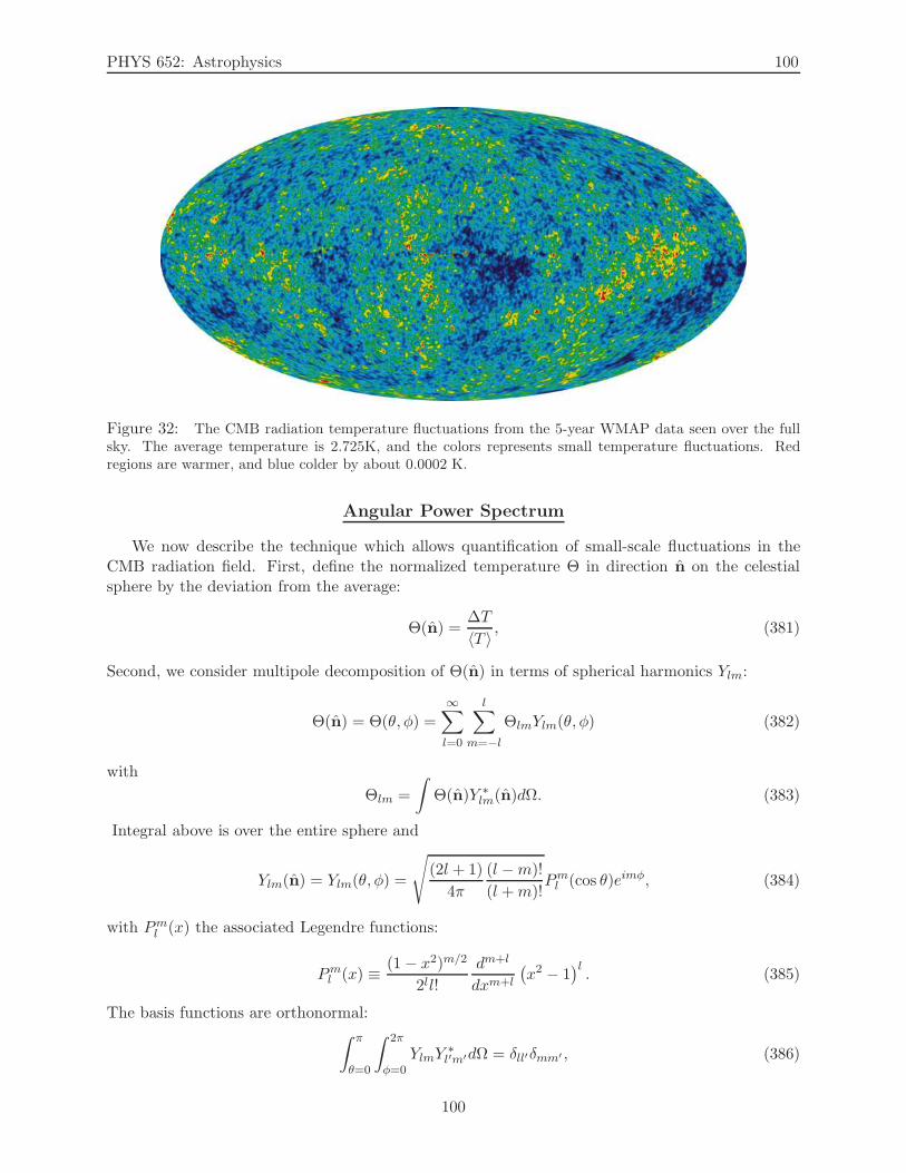
PHYS 652: Astrophysics 100
Figure 32: The CMB radiation temperature fluctuations from the 5-year WMAP data seen over the fullsky. The average temperature is 2.725K, and the colors represents small temperature fluctuations. Redregions are warmer, and blue colder by about 0.0002 K.
Angular Power Spectrum
We now describe the technique which allows quantification of small-scale fluctuations in theCMB radiation field. First, define the normalized temperature Θ in direction n on the celestialsphere by the deviation from the average:
Θ(n) =∆T
〈T 〉 , (381)
Second, we consider multipole decomposition of Θ(n) in terms of spherical harmonics Ylm:
Θ(n) = Θ(θ, φ) =∞∑
l=0
l∑
m=−lΘlmYlm(θ, φ) (382)
with
Θlm =
∫
Θ(n)Y ∗lm(n)dΩ. (383)
Integral above is over the entire sphere and
Ylm(n) = Ylm(θ, φ) =
√
(2l + 1)
4π
(l −m)!
(l +m)!Pml (cos θ)eimφ, (384)
with Pml (x) the associated Legendre functions:
Pml (x) ≡ (1− x2)m/2
2ll!
dm+l
dxm+l
(
x2 − 1)l. (385)
The basis functions are orthonormal:∫ π
θ=0
∫ 2π
φ=0YlmY
∗l′m′dΩ = δll′δmm′ , (386)
100
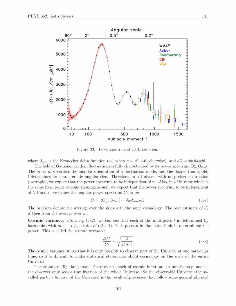
PHYS 652: Astrophysics 101
Figure 33: Power spectrum of CMB radiation.
where δnn′ is the Kronecker delta function (=1 when n = n′, =0 otherwise), and dΩ = sin θdφdθ.The field of Gaussian random fluctuations is fully characterized by its power spectrum Θ∗
lmΘl′m′ .The order m describes the angular orientation of a fluctuation mode, and the degree (multipole)l determines its characteristic angular size. Therefore, in a Universe with no preferred direction(isotropic), we expect that the power spectrum to be independent of m. Also, in a Universe which isthe same from point to point (homogeneous), we expect that the power spectrum to be independentof l. Finally, we define the angular power spectrum Cl to be
Cl = 〈Θ∗lmΘl′m′〉 = δll′δmm′Cl. (387)
The brackets denote the average over the skies with the same cosmology. The best estimate of Clis then from the average over m.
Cosmic variance. From eq. (382), we can see that each of the multipoles l is determined byharmonics with m ∈ [−l, l], a total of (2l + 1). This poses a fundamental limit in determining thepower. This is called the cosmic variance:
∆ClCl
=
√
2
2l + 1. (388)
The cosmic variance states that it is only possible to observe part of the Universe at one particulartime, so it is difficult to make statistical statements about cosmology on the scale of the entireUniverse.
The standard Big Bang model features an epoch of cosmic inflation. In inflationary models,the observer only sees a tiny fraction of the whole Universe. So the observable Universe (the so-called particle horizon of the Universe) is the result of processes that follow some general physical
101
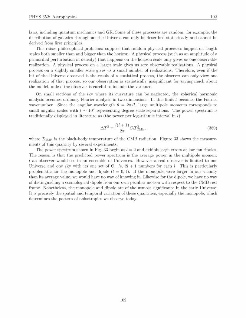
PHYS 652: Astrophysics 102
laws, including quantum mechanics and GR. Some of these processes are random: for example, thedistribution of galaxies throughout the Universe can only be described statistically and cannot bederived from first principles.
This raises philosophical problems: suppose that random physical processes happen on lengthscales both smaller than and bigger than the horizon. A physical process (such as an amplitude of aprimordial perturbation in density) that happens on the horizon scale only gives us one observablerealization. A physical process on a larger scale gives us zero observable realizations. A physicalprocess on a slightly smaller scale gives us a small number of realizations. Therefore, even if thebit of the Universe observed is the result of a statistical process, the observer can only view onerealization of that process, so our observation is statistically insignificant for saying much aboutthe model, unless the observer is careful to include the variance.
On small sections of the sky where its curvature can be neglected, the spherical harmonicanalysis becomes ordinary Fourier analysis in two dimensions. In this limit l becomes the Fourierwavenumber. Since the angular wavelength θ = 2π/l, large multipole moments corresponds tosmall angular scales with l ∼ 102 representing degree scale separations. The power spectrum istraditionally displayed in literature as (the power per logarithmic interval in l)
∆T 2 ≡ l(l + 1)
2πClT
2CMB, (389)
where TCMB is the black-body temperature of the CMB radiation. Figure 33 shows the measure-ments of this quantity by several experiments.
The power spectrum shown in Fig. 33 begin at l = 2 and exhibit large errors at low multipoles.The reason is that the predicted power spectrum is the average power in the multipole momentl an observer would see in an ensemble of Universes. However a real observer is limited to oneUniverse and one sky with its one set of Θlm’s, 2l + 1 numbers for each l. This is particularlyproblematic for the monopole and dipole (l = 0, 1). If the monopole were larger in our vicinitythan its average value, we would have no way of knowing it. Likewise for the dipole, we have no wayof distinguishing a cosmological dipole from our own peculiar motion with respect to the CMB restframe. Nonetheless, the monopole and dipole are of the utmost significance in the early Universe.It is precisely the spatial and temporal variation of these quantities, especially the monopole, whichdetermines the pattern of anisotropies we observe today.
102
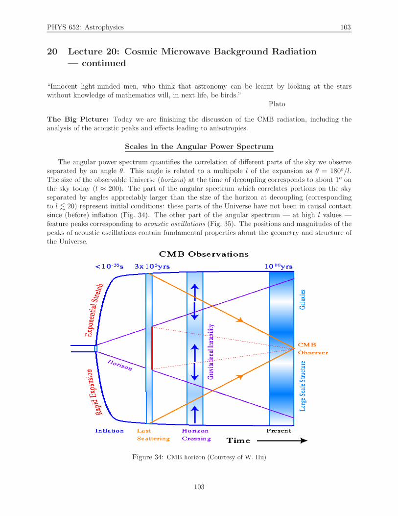
PHYS 652: Astrophysics 103
20 Lecture 20: Cosmic Microwave Background Radiation— continued
“Innocent light-minded men, who think that astronomy can be learnt by looking at the starswithout knowledge of mathematics will, in next life, be birds.”
Plato
The Big Picture: Today we are finishing the discussion of the CMB radiation, including theanalysis of the acoustic peaks and effects leading to anisotropies.
Scales in the Angular Power Spectrum
The angular power spectrum quantifies the correlation of different parts of the sky we observeseparated by an angle θ. This angle is related to a multipole l of the expansion as θ = 180o/l.The size of the observable Universe (horizon) at the time of decoupling corresponds to about 1o onthe sky today (l ≈ 200). The part of the angular spectrum which correlates portions on the skyseparated by angles appreciably larger than the size of the horizon at decoupling (correspondingto l . 20) represent initial conditions: these parts of the Universe have not been in causal contactsince (before) inflation (Fig. 34). The other part of the angular spectrum — at high l values —feature peaks corresponding to acoustic oscillations (Fig. 35). The positions and magnitudes of thepeaks of acoustic oscillations contain fundamental properties about the geometry and structure ofthe Universe.
Figure 34: CMB horizon (Courtesy of W. Hu)
103
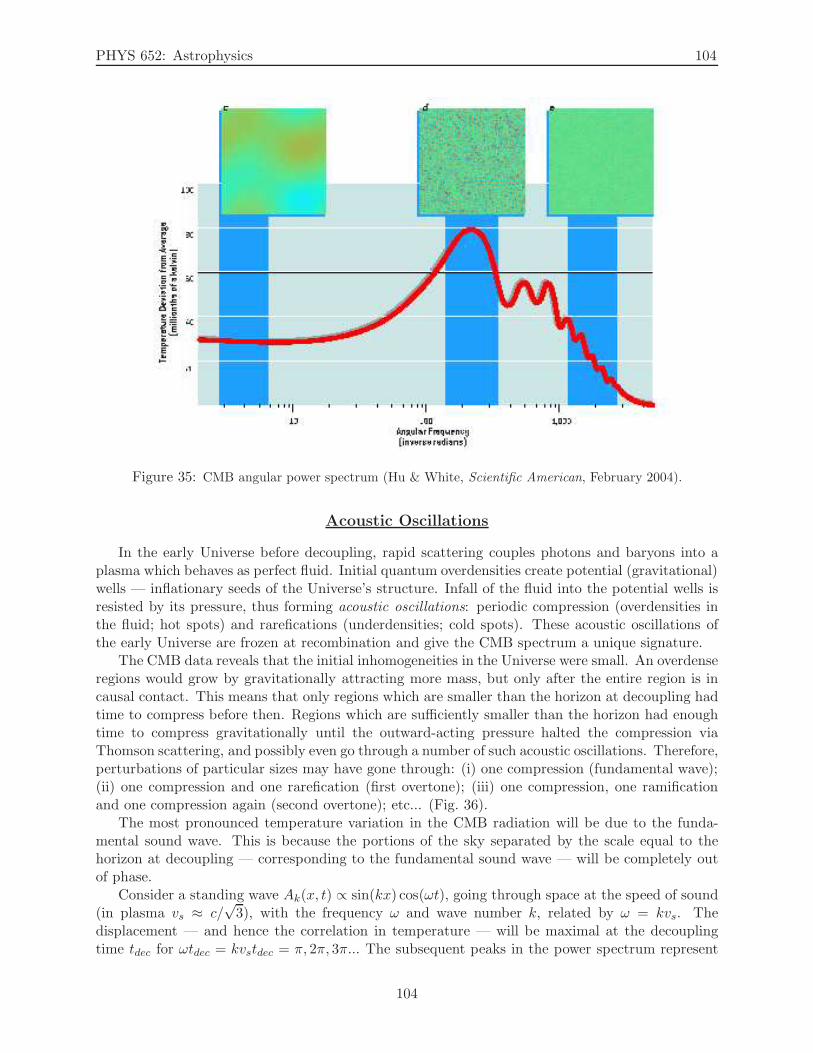
PHYS 652: Astrophysics 104
Figure 35: CMB angular power spectrum (Hu & White, Scientific American, February 2004).
Acoustic Oscillations
In the early Universe before decoupling, rapid scattering couples photons and baryons into aplasma which behaves as perfect fluid. Initial quantum overdensities create potential (gravitational)wells — inflationary seeds of the Universe’s structure. Infall of the fluid into the potential wells isresisted by its pressure, thus forming acoustic oscillations: periodic compression (overdensities inthe fluid; hot spots) and rarefications (underdensities; cold spots). These acoustic oscillations ofthe early Universe are frozen at recombination and give the CMB spectrum a unique signature.
The CMB data reveals that the initial inhomogeneities in the Universe were small. An overdenseregions would grow by gravitationally attracting more mass, but only after the entire region is incausal contact. This means that only regions which are smaller than the horizon at decoupling hadtime to compress before then. Regions which are sufficiently smaller than the horizon had enoughtime to compress gravitationally until the outward-acting pressure halted the compression viaThomson scattering, and possibly even go through a number of such acoustic oscillations. Therefore,perturbations of particular sizes may have gone through: (i) one compression (fundamental wave);(ii) one compression and one rarefication (first overtone); (iii) one compression, one ramificationand one compression again (second overtone); etc... (Fig. 36).
The most pronounced temperature variation in the CMB radiation will be due to the funda-mental sound wave. This is because the portions of the sky separated by the scale equal to thehorizon at decoupling — corresponding to the fundamental sound wave — will be completely outof phase.
Consider a standing wave Ak(x, t) ∝ sin(kx) cos(ωt), going through space at the speed of sound(in plasma vs ≈ c/
√3), with the frequency ω and wave number k, related by ω = kvs. The
displacement — and hence the correlation in temperature — will be maximal at the decouplingtime tdec for ωtdec = kvstdec = π, 2π, 3π... The subsequent peaks in the power spectrum represent
104
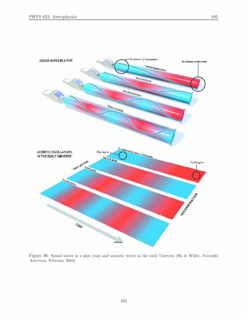
PHYS 652: Astrophysics 105
Figure 36: Sound waves in a pipe (top) and acoustic waves in the early Universe (Hu & White, ScientificAmerican, February 2004).
105
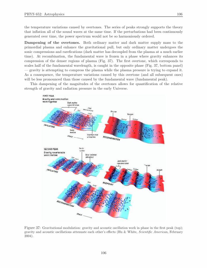
PHYS 652: Astrophysics 106
the temperature variations caused by overtones. The series of peaks strongly supports the theorythat inflation all of the sound waves at the same time. If the perturbations had been continuouslygenerated over time, the power spectrum would not be so harmoniously ordered.
Dampening of the overtones. Both ordinary matter and dark matter supply mass to theprimordial plasma and enhance the gravitational pull, but only ordinary matter undergoes thesonic compressions and rarefications (dark matter has decoupled from the plasma at a much earliertime). At recombination, the fundamental wave is frozen in a phase where gravity enhances itscompression of the denser regions of plasma (Fig. 37). The first overtone, which corresponds toscales half of the fundamental wavelength, is caught in the opposite phase (Fig. 37, bottom panel)— gravity is attempting to compress the plasma while the plasma pressure is trying to expand it.As a consequence, the temperature variations caused by this overtone (and all subsequent ones)will be less pronounced than those caused by the fundamental wave (fundamental peak).
This dampening of the magnitudes of the overtones allows for quantification of the relativestrength of gravity and radiation pressure in the early Universe.
Figure 37: Gravitational modulation: gravity and acoustic oscillation work in phase in the first peak (top);gravity and acoustic oscillations attenuate each other’s effects (Hu & White, Scientific American, February2004).
106
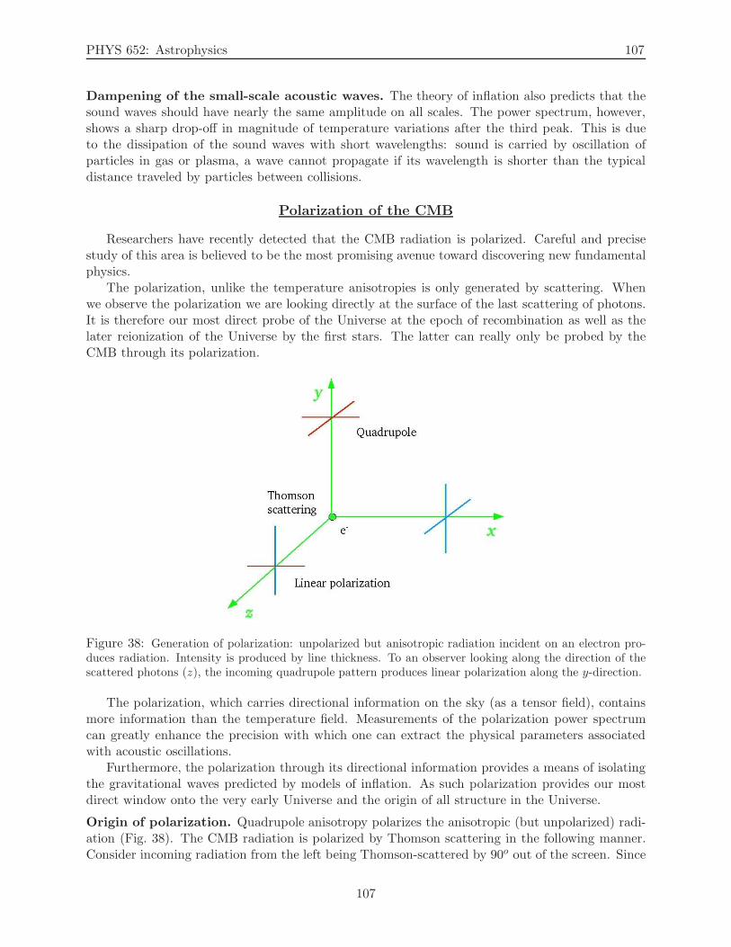
PHYS 652: Astrophysics 107
Dampening of the small-scale acoustic waves. The theory of inflation also predicts that thesound waves should have nearly the same amplitude on all scales. The power spectrum, however,shows a sharp drop-off in magnitude of temperature variations after the third peak. This is dueto the dissipation of the sound waves with short wavelengths: sound is carried by oscillation ofparticles in gas or plasma, a wave cannot propagate if its wavelength is shorter than the typicaldistance traveled by particles between collisions.
Polarization of the CMB
Researchers have recently detected that the CMB radiation is polarized. Careful and precisestudy of this area is believed to be the most promising avenue toward discovering new fundamentalphysics.
The polarization, unlike the temperature anisotropies is only generated by scattering. Whenwe observe the polarization we are looking directly at the surface of the last scattering of photons.It is therefore our most direct probe of the Universe at the epoch of recombination as well as thelater reionization of the Universe by the first stars. The latter can really only be probed by theCMB through its polarization.
Figure 38: Generation of polarization: unpolarized but anisotropic radiation incident on an electron pro-duces radiation. Intensity is produced by line thickness. To an observer looking along the direction of thescattered photons (z), the incoming quadrupole pattern produces linear polarization along the y-direction.
The polarization, which carries directional information on the sky (as a tensor field), containsmore information than the temperature field. Measurements of the polarization power spectrumcan greatly enhance the precision with which one can extract the physical parameters associatedwith acoustic oscillations.
Furthermore, the polarization through its directional information provides a means of isolatingthe gravitational waves predicted by models of inflation. As such polarization provides our mostdirect window onto the very early Universe and the origin of all structure in the Universe.
Origin of polarization. Quadrupole anisotropy polarizes the anisotropic (but unpolarized) radi-ation (Fig. 38). The CMB radiation is polarized by Thomson scattering in the following manner.Consider incoming radiation from the left being Thomson-scattered by 90o out of the screen. Since
107
PHYS 652: Astrophysics 108
light cannot be polarized along its direction of motion, only one linear polarization gets Thomson-scattered. However, there is nothing special about light coming in from the left: if the light alsocomes from the top, the resulting scattered radiation will have both polarization states. The degreeof polarization will depend on intensity of the incoming radiation, so the 90o anisotropies in theradiation will result in linear polarization (Fig. 38).
Shift to high l. Because the polarization arises from scattering, which in turn dilutes thequadrupole, the anisotropies in polarization are much weaker than anisotropies in temperature.With each scatter that the photon experiences on as it approaches equilibrium, the polarizationis reduced. The remaining polarization is a direct result of the stoppage of scattering. The localquadrupole on the scales which are much larger than the mean-free path of photons (for instance,the scale of the horizon) will be diluted by multiple scattering, and therefore not dominant in thespectrum. The peak of the spectrum is shifted toward smaller scales (large l values), where thelocal quadrupole is close to the mean-free path of photons.
Physical Effects Affecting the CMB Radiation
The Sunyaev–Zel’dovich Effect. The Sunyaev-Zel’dovich (SZ) effect refers to the Comptonscattering of CMB photons by hot, ionized gas in clusters of galaxies. It was first predicted in1969 by Sunyaev and Zel’dovich. The effect is a foreground anisotropy to the CMB. The SZ effectcauses a “hotspot” in the CMB due to the kinetic SZ effect (due to the bulk motion of the clusterwith respect to the CMB) and a noticeable change in the shape of the CMB spectrum due to thethermal SZ effect.
The SZ effect is important to the study of cosmology and the CMB for two main reasons:
1. the observed “hotspots” created by the kinetic effect will distort the power spectrum of CMBanisotropies. These need to be separated from the primary anisotropies in order to probeproperties of inflation.
2. The thermal SZ effect can be measured and combined with X-ray observations in order todetermine values of cosmological parameters, in particular the present value of the Hubblerate H0.
Interaction between photons of the CMB and charged particles they encounter as they passthrough the hot, ionized gas in clusters of galaxies causes them to scatter, thus polarizing the CMBradiation across wide swaths of the sky. Observations of this large-angle polarization by the WMAPspacecraft imply that about 17 percent of the CMB photons were scattered by a thin fog of ionizedgas a few hundred million years after the Big Bang.
This relatively large fraction is perhaps the biggest surprise from the WMAP data. Cosmologistshad previously theorized that most of the Universes hydrogen and helium would have been ionizedby the radiation from the first stars, which were extremely massive and bright. (This process iscalled reionization because it returned the gases to the plasma state that existed before the emissionof the CMB.) But the theorists estimated that this event occurred nearly a billion years after theBig Bang, and therefore only about 5 percent of the CMB photons would have been scattered.WMAPs evidence of a higher fraction indicates a much earlier reionization and presents a challengefor the modeling of the first rounds of star formation. The discovery may even challenge the theoryof inflations prediction that the initial density fluctuations in the primordial Universe were nearlythe same at all scales. The first stars might have formed sooner if the small-scale fluctuations hadhigher amplitudes. The WMAP data also contain another hint of deviation from scale invariancethat was first observed by the COBE satellite. On the biggest scales, corresponding to regions
108
PHYS 652: Astrophysics 109
stretching more than 60 degrees across the sky, both WMAP and COBE found a curious lack oftemperature variations in the CMB. This deficit may well be a statistical fluke: because the sky isonly 360 degrees around, it may not contain enough large-scale regions to make an adequate samplefor measuring temperature variations. But some theorists have speculated that the deviation mayindicate inadequacies in the models of inflation, dark energy or the topology of the Universe.
Sachs-Wolfe Effect. At last scattering the baryons and photons decouple and the photons sud-denly find themselves free to travel in straight paths through the Universe. However, the baryonsare clustered together in gravitational potential wells prior to last scattering. Since the photons aretightly coupled to the baryons before last scattering, they are confined to potential wells too. Thusthe photons have to climb out of potential wells when they are suddenly freed at last scattering.This climb requires some energy and the photons are therefore redshifted. The subsequent rise atlow l in the CMB power spectrum is known as the Sachs-Wolfe (SW) effect, and since it is imprintedon the CMB power spectrum at the time of last scattering, it is considered a primary anisotropy.
This effect is the predominant source of fluctuations in the CMB for angular scales above aboutten degrees — the regions in the early Universe which were too big to undergo acoustic oscillations.
Integrated Sachs-Wolfe Effect. The Integrated Sachs-Wolfe (ISW) effect is also caused bygravitational redshift, however here it occurs between the surface of last scattering and the Earth,so it is not a fundamental part of the CMB.
The ISW effect can arise after last scattering as the photons free stream through the Universe.Although the photons are no longer tightly coupled to the baryons, they can still slip into potentialwells and have to climb back out. When they fall in, the photons gain some energy (are blueshifted)and when they climb back out, they are redshifted. Assuming that the depth of the potential wellremains constant while the photon traverses it, the redshift exactly cancels the blueshift. No traceof the photon’s passage through the potential well remains, assuming that both sides of the dip arethe same height and no energy is dissipated. Suppose, however, that the potential well throughwhich the photon passes either decays or deepens while the photon is inside. Then its redshift andblueshift will not exactly cancel; instead the photon gains or loses some energy (respectively) fromits passage through the potential well.
There are two main contributions to the integrated effect. The first occurs shortly after photonsleave the last scattering surface, and is due to the evolution of the potential wells as the Universechanges from being dominated by radiation to being dominated by matter. The second, sometimescalled the ‘late-time integrated Sachs-Wolfe effect’, arises much later as the evolution starts tofeel the effect of the cosmological constant (or, more generally, dark energy), or curvature of theUniverse if it is not flat. The latter effect has an observational signature in the amplitude of thelarge scale perturbations of the CMB and their correlation with the large scale structure.
The primary anisotropies (SW) on the CMB power spectrum tell us about the initial conditionsof the photons, and any passage through a potential well that results in a net energy loss or gainchanges these conditions and leaves a mark on the spectrum — the secondary anisotropy (ISW).
Determining the Cosmic Parameters from CMB Radiation
Baryonic matter content (Ωb). Relative magnitudes of the first overtone to the fundamentalpeak in the power spectrum of the CMB radiation enables precise quantification of relative strengthsof gravity and radiation in the early Universe. It has been determined that the energy in baryonswas about the same as the energy in CMB photons at the time of decoupling, which — throughscaling which we have done in previous classes (recall ργ ∝ a4) — puts the baryonic content of theUniverse at about 5 percent. This is in excellent agreement with the predictions of the BBN.
109
PHYS 652: Astrophysics 110
Dark energy (ΩΛ). Because dark energy accelerates the expansion of the Universe, it weakensthe gravitational-potential wells associated with galaxy clustering (ISW effect). These effects canare detected and quantified at the large-scale variations of the CMB radiation (low l values).
Hubble rate (H0). SZ effect is used to measure the present-day value of the Hubble rate (H0).
110
PHYS 652: Astrophysics 111
21 Lecture 21: The Schwarzschild Metric and Black Holes
“All of physics is either impossible or trivial. It is impossible until you understand it, and then itbecomes trivial.”
Ernest Rutherford
The Big Picture: Today we are starting the third (and last) part of the course: black holes,stars and galaxies. We show that the Einstein’s field equations imply the existence of a space-timesingularity, which we now know as “black holes”.
The Schwarzschild Problem
Shortly after Einstein published his field equations of GR, Karl Schwarzschild solved them tofind the space-time geometry outside a stationary, spherical distribution of matter of mass M .Since the space outside the distribution is empty, the energy-momentum tensor Tαβ vanishes, sothe Einstein’s field equation becomes:
Rαβ −1
2gαβR = 0, (390)
with an appropriate metric tensor. The appropriate boundary conditions are:
1. metric must match interior metric at the body’s surface;
2. metric must go to the flat (Minkowski) metric far away from the body.
We now solve for the Schwarzschild metric gαβ which solves the Schwarzschild problem. We startwith a general static and isotropic metric:
1. static: both time-independent and symmetric under time reversal(only time-independent ⇐⇒ stationary);
2. isotropic: invariant under spatial rotations (same in all directions).
The interval satisfying these criteria may be written as
ds2 = −A(r)dt2 +B(r)dr2 + r2(
dθ2 + sin2 θdφ2)
, (391)
where the first two term on the RHS describe radial behavior (isotropy), and the last two thesurface of the sphere (spherical symmetry). It can be expressed in many equivalent forms. Oneconvenient form is:
ds2 = −eN(r)dt2 + eP (r)dr2 + r2(
dθ2 + sin2 θdφ2)
, (392)
corresponding to the metric tensor
gαβ =
−eN(r) 0 0 0
0 eP (r) 0 00 0 r2 00 0 0 r2 sin2 θ
. (393)
The Schwarzschild problem reduces to solving for N(r) and P (r) from Einstein’s field equationsand the appropriate boundary conditions.
111
PHYS 652: Astrophysics 112
Solving the Schwarzschild Problem
Earlier we have defined an alternative Lagrangian [eq. 26]:
L =1
2gαβ x
αxβ, (394)
(where dot denotes s-derivative) which for the metric in eq. (393) becomes (x0 → t, x1 → r, x2 → θ,x3 → φ):
L = −1
2eN t2 +
1
2eP r2 +
1
2r2θ2 +
1
2r2 sin2 θφ2, (395)
This alternative Lagrangian allows us to easily read off Christoffel symbols by comparing it to thegeodesic equation [eq. (31)]:
d2xν
ds2+ Γνγδ
dxγ
ds
dxδ
ds= 0, (396)
which we can combine to obtain the Riemann and Ricci tensors. Let us solve the Lagrange equations
∂L
∂xα− d
ds
∂L
∂xα= 0,
for each of the components of the space-time (′ denotes r-derivative):
• t-component:
∂L
∂t− d
ds
(
∂L
∂t
)
= 0
0− d
ds
(
−eN t)
= 0
eNdN
dr
dr
dst+ eN t = 0
eN(
t+N ′tr)
= 0
=⇒ d2t
ds2+N ′
(
dt
ds
)(
dr
ds
)
= 0. (397)
After comparing it to eq. (396), we obtain
d2t
ds2+(
Γ001 + Γ0
10
)
(
dt
ds
)(
dr
ds
)
= 0, (398)
which means that (because of symmetry of the Christoffel symbols: Γαβγ = Γαγβ)
Γ001 = Γ0
10 =1
2N ′, (399)
while other Γ0αβ symbols vanish.
112
PHYS 652: Astrophysics 113
• r-component:
∂L
∂r− d
ds
(
∂L
∂r
)
= 0
−1
2N ′eN t2 +
1
2P ′eP r2 + rθ2 + r sin2 θφ2 − d
ds
(
eP r)
= 0
−1
2N ′eN t2 +
1
2P ′eP r2 + rθ2 + r sin2 θφ2 − ePP ′r2 − eP r = 0
−eP(
r +1
2N ′eN−P t2 +
1
2P ′r2 − e−P rθ2 − e−P r sin2 θφ2
)
= 0
d2r
ds2+
1
2N ′eN−P
(
dt
ds
)2
+1
2P ′(
dr
ds
)2
− e−P r
(
dθ
ds
)2
− e−P r sin2 θ
(
dφ
ds
)2
= 0. (400)
After comparing it to eq. (396), we obtain
d2r
ds2+ Γ1
00
(
dt
ds
)2
+ Γ111
(
dr
ds
)2
+ Γ122
(
dθ
ds
)2
+ Γ133
(
dφ
ds
)2
= 0, (401)
which means that
Γ100 =
1
2N ′eN−P ,
Γ111 =
1
2P ′,
Γ122 = −e−P r,
Γ133 = −e−P r sin2 θ,
(402)
while other Γ1αβ symbols vanish.
• θ-component:
∂L
∂θ− d
ds
(
∂L
∂θ
)
= 0
1
2r22 sin θ cos θφ2 − d
ds
(
r2θ)
= 0
1
2r2 sin 2θφ2 − 2rrθ − r2θ = 0
−r2(
θ − 1
2sin 2θφ2 + 2
r
rθ
)
= 0
d2θ
ds2+
2
r
(
dr
ds
)(
dθ
ds
)
− 1
2sin 2θ
(
dφ
ds
)2
= 0 (403)
After comparing it to eq. (396), we obtain
d2θ
ds2+(
Γ212 + Γ2
21
)
(
dr
ds
)(
dθ
ds
)
+ Γ233
(
dφ
ds
)2
= 0, (404)
which means that
Γ212 = Γ2
21 =1
r,
Γ233 = −1
2sin 2θ,
(405)
113
PHYS 652: Astrophysics 114
while other Γ2αβ symbols vanish.
• φ-component:
∂L
∂φ− d
ds
(
∂L
∂φ
)
= 0
0− d
ds
(
r2 sin2 θφ)
= 0
−2rr sin2 θφ− 2r2 sin θ cos θθφ− r2 sin2 θφ = 0
−r2 sin2 θ
(
φ+ 2r
rφ+ 2
cos θ
sin θθφ
)
= 0
d2φ
ds2+
2
r
(
dr
ds
)(
dφ
ds
)
+ 2cot θ
(
dθ
ds
)(
dφ
ds
)
= 0 (406)
After comparing it to eq. (396), we obtain
d2φ
ds2+(
Γ313 + Γ3
31
)
(
dr
ds
)(
dφ
ds
)
+(
Γ323 + Γ3
32
)
(
dθ
ds
)(
dφ
ds
)
= 0, (407)
which means that
Γ313 = Γ3
31 =1
r,
Γ323 = Γ3
32 = cot θ,
(408)
while other Γ3αβ symbols vanish.
These Christoffel symbols associated with the metric given in eq. (393) are needed to computethe Riemann tensor, which, in turn, is used to compute the Ricci tensor and Ricci scalar, to fullydetermine the LHS of the Einstein’s equation: Gαβ ≡ Rαβ − 1
2gαβR = 0.It can be shown (Homework set #3) that Gαβ = 0 leads to
−eN−P
r
(
P ′ − 1
r
)
−−eN
r2= 0,
−N ′
r− 1
r2(
1− eP)
= 0,
−1
2r2e−P
[
N ′′ − 1
2P ′N ′ +
1
2
(
N ′)2 +N ′ − P ′
r
]
= 0. (409)
These expressions combine to give (Homework set #3) to obtain
dP
dr= −dN
dr=
1
r
(
1− eP)
,
which can be solved for P :∫
dP
1− eP=
∫
dr
r∫(
1− eP
1− eP+
eP
1− eP
)
dP = lnCr
P − ln(
1− eP)
= ln eP − ln(
1− eP)
= lneP
1− eP= lnCr
eP
1− eP= Cr =⇒ eP =
Cr
1 + Cr(410)
114
PHYS 652: Astrophysics 115
Solving for N we obtainN = −P + const. =⇒ eN = econste−P , (411)
but since we have to recover Minkowski metric at large distances:
limr→∞
g00 → −1,
limr→∞
g11 → 1, (412)
and const. = 0. Therefore,
N = −P
g00 = −eN = −e−P = − 1
g11= −
(
1 + Cr
Cr
)
= −(
1 +1
Cr
)
. (413)
For weak gravitational fields, we derived in eq. (39) including the constants:
g00 = −(
1 +2Φ
c2
)
= −(
1− 2GM
rc2
)
= − 1
g11=⇒ C = − c2
2GM. (414)
We finally arrive at the solution to the Schwarzschild problem, and the corresponding line elementin the Schwarzschild metric (with constants c and G included explicitly):
ds2 = −(
1− 2GM
rc2
)
c2dt2 +dr2
1− 2GMrc2
+ r2dθ2 + r2 sin2 θdφ2. (415)
Birkhoff’s theorem. The derivation of the Schwarzschild metric does not require any otherinformation about the distribution of the matter giving rise to the gravitational field — it onlyrequires that it is:
• spherically symmetric;
• that it has zero density at the radius of interest.
Birkhoff showed that any spherically symmetric vacuum solution of Einstein’s field equations mustalso be static and agree with Schwarzschild’s solution. Therefore, the spherically symmetric massleads to the Schwarzschild metric regardless of whether the mass is static, collapsing, expandingor pulsating. This, of course, refers to the field outside the mass, as first stated in the derivation,because we start with Tαβ = 0. Two of the most important features of Newtonian gravity thereforeapply to GR:
• the gravity of a spherical body appears to act from a central point mass;
• the gravitational field inside a spherical shell vanishes.
Schwarzschild Radius, Event Horizon and Black Holes
The Schwarzschild space-time metric has a singularity when the denominator in the secondterm is equal to zero:
1− 2GM
c2r= 0, (416)
115
PHYS 652: Astrophysics 116
which happens when the radius associated with mass M is
rs =2GM
c2. (417)
This is called the Schwarzschild radius, or the event horizon, because events occurring inside itcannot propagate light signals to the outside. Any body which is small enough to exist withinits own event horizon is therefore disconnected from the rest of the Universe: its only physicalmanifestation is through its (infinitely) deep gravitational potential well, which is what led to theadoption of the term black hole in the late 1960’s.
For a body with mass equal to that of our Sun, the event horizon is equal to
rs =2GM⊙
c2=
2(
6.67 × 10⁻⁸) (
2× 1033)
(3× 10¹⁰)2≈ 3× 105cm = 3 km. (418)
We can write the proper time in the Schwarzschild metric as
ds2 = −dτ2 =⇒ dτ2 =
(
1− 2GM
c2r
)
dt2 − dr2
1− 2GMc2r
− r2dθ2 − r2 sin2 θdφ2, (419)
where dt is the time interval according to an observer at r → ∞, and dτ is the time intervalmeasured by a local observer (in comoving coordinates, in which the Universe is static). Becausefor the local observer the Universe is static, it means that dr = 0, so
dt2 =dτ2
1− 2GMc2r
. (420)
This is time dilation: while the local observer near the black hole (at r & rs) sees nothing unusualabout her/his time-measurements (dτ), the measurements of the observer at r → ∞ would suggest
that the local observer’s clock runs slow by a factor(
1− 2GMc2r
)−1/2. It becomes infinitely slow at
the event horizon rs. Therefore, the inertial observer (at infinity) can never witness the infallingobserver reach the event horizon.
Orbits in Schwarzschild’s Geometry
For the dynamics of black holes and their accretion disks, it is important to quantify the motionof particles which find themselves near the black hole. We now present a brief exposition of theorbit theory near a black hole.
In order to compute orbits in Schwarzschild’s geometry, we need to first compute the equationsof motion.
Combining components of the solutions to Einstein’s equation in Schwarzschild’s metric whichwe just derived with the general property of massive particles in a metric
gαβdxα
ds
dxβ
ds= 1, (421)
(= 0 for photons), it can be shown that the motion near the black hole can be described with
(
dr
dτ
)2
= B2 −(
1− A2
r2
)
(
1− rsr
)
dφ
dτ=
A
r2, (422)
116
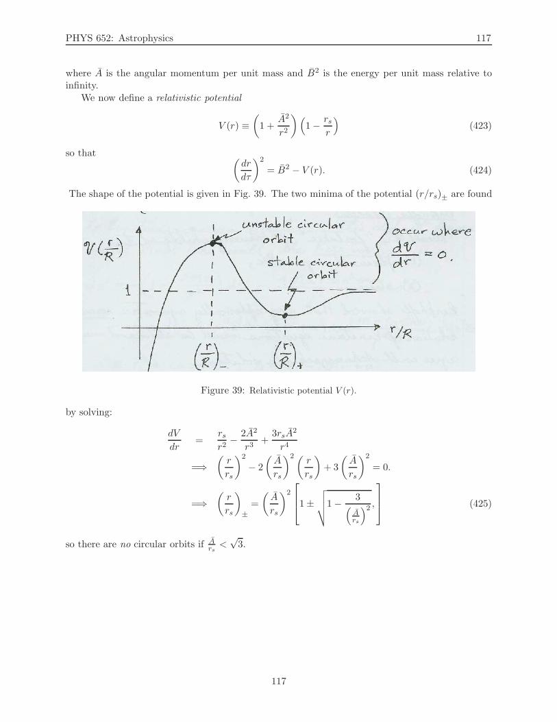
PHYS 652: Astrophysics 117
where A is the angular momentum per unit mass and B2 is the energy per unit mass relative toinfinity.
We now define a relativistic potential
V (r) ≡(
1 +A2
r2
)
(
1− rsr
)
(423)
so that(
dr
dτ
)2
= B2 − V (r). (424)
The shape of the potential is given in Fig. 39. The two minima of the potential (r/rs)± are found
Figure 39: Relativistic potential V (r).
by solving:
dV
dr=
rsr2
− 2A2
r3+
3rsA2
r4
=⇒(
r
rs
)2
− 2
(
A
rs
)2(r
rs
)
+ 3
(
A
rs
)2
= 0.
=⇒(
r
rs
)
±=
(
A
rs
)2
1±
√
√
√
√
1− 3(
Ars
)2 ,
(425)
so there are no circular orbits if Ars
<√3.
117
PHYS 652: Astrophysics 118
22 Lecture 22: Degeneracy of Matter
“Physics is very muddled again at the moment; it is much too hard for me anyway, and I wish Iwere a movie comedian or something like that and had never heard anything about physics!”
Wolfgang Pauli
The Big Picture: Last time we derived the Schwarzschild metric corresponding to an isolatedmass, which led to the the introduction of black holes and even horizons. Today we introducedegenerate matter, such as the matter in white dwarfs and neutron stars. We also introducepolytropes as simple equilibrium stellar models.
Degeneracy
According to Pauli’s Exclusion Principle, no two fermions (particles with spin of one half) canoccupy the same quantum state. This is equivalent to requiring that the volume per fermion beproportional to λ3
c ∼ (~/mc)3, where m is the fermion’s mass and λc is its Compton wavelength.The average number density of the fermions is therefore nf ∼ λ−3
c . In white dwarfs the density isnf times the mass per electron, and in neutron stars it is the nucleon mass times nf .
We can use this argument to compute the relative densities of white dwarfs, which are supportedby electron degeneracy, and neutron stars, supported by neutron degeneracy to obtain (with ap-proximation that the mass per electron is on the order of magnitude of the mass of the nucleon):
ρnsρwd
=λ−3n,e
λ−3c,e
=m3n
m3e
=
(
mn
me
)3
≈ (2000)3 = 8× 10⁹. (426)
In a gas of very high fermion density, the lower momentum states are filled, so fermions mustthen occupy states of higher momentum. These high-momentum fermions make a large contributionto the pressure, and the gas is said to be (partially) “degenerate”.
Complete Degeneracy
If the fermion density is large enough, then essentially all available states having energies E <ǫf (where ǫf is the Fermi energy, defined as the energy of the highest occupied quantum statein a system of fermions at absolute zero temperature). As the gas temperature is lowered, thedistribution function
f(p) =1
e[E(p)−µ]/T + 1, (427)
approaches unity for particle energies E . µ, and zero for E & µ, where µ is the chemical potential.For T = 0, µ ≡ ǫf , so the distribution function becomes a step function:
f(p) = θ(ǫf − E(p)) =
1 if ǫf ≥ E(p),0 if ǫf < E(p).
(428)
The number density of fermions corresponding to the distribution function above is
n = g
∫ ∞
0f(p)
d3p
(2π~)3= 2
∫ pf
0
4πp2dp
(2π~)3=
8π
h3
∫ pf
0p2dp =
8π
h31
3p3f =
8π
3h3p3f , (429)
so
pf =
(
3h3
8πn
)1/3
. (430)
118
PHYS 652: Astrophysics 119
pf is the Fermi momentum corresponding to the Fermi energy:
ǫf =p2f2m
=⇒ pf =√
2mǫf . (431)
The energy density is given by
ρe = g
∫ ∞
0E(p)f(p)
d3p
h3=
8π
h3
∫ pf
0E(p)p2dp, (432)
where E(p) is the kinetic energy per fermion.
Nonrelativistic (complete) degeneracy. When the fermions are nonrelativistic, so p = mvand E(p) = p2/2m. The energy density then is
ρ =8π
h3
∫ pf
0
p2
2mp2dp =
8π
2mh3
∫ pf
0p4dp =
8π
2mh31
5p5f =
8π
5h3p3f
p2f2m
=8π
5h3
(
3h3
8πn
)
ǫf
=⇒ ρ =3
5nǫf . (433)
For nonrelativistic particles
P =2
3ρ =
2
3
3
5nǫf =
2
5np2f2m
=n
5mp2f =
n
5m
(
3h3
8πn
)2/3
=h2
20m
(
3
π
)2/3
n5/3. (434)
The equation above is the equation of state for a nonrelativistic, completely degenerate fermiongas.
Extreme relativistic (complete) degeneracy. When the fermions are relativistic, p ≫ mc andE(p) = c
√
p2 +m2c2 ≈ cp. The energy density then is
ρ =8π
h3
∫ pf
0cpp2dp =
8πc
h3
∫ pf
0p3dp =
8πc
h31
4p4f =
2π
h3p3f (cpf ) =
2π
h3
(
3h3
8πn
)
ǫf .
=⇒ ρ =3
4nǫf . (435)
For relativistic particles (recall Homework set #1):
P =1
3ρ =
1
3
3
4nǫf =
1
4ncpf =
1
4nc
(
3h3
8πn
)1/3
=hc
8
(
3
π
)1/3
n4/3. (436)
The equation above is the equation of state for an extreme relativistic, completely degeneratefermion gas.Important point: For complete or nearly complete degeneracy, the pressure P is independent ofthe temperature T .
Onset of Degeneracy
We now estimate the thresholds for the onset of the complete nonrelativistic degeneracy andcomplete relativistic degeneracy.
119

PHYS 652: Astrophysics 120
• From nondegeneracy to complete nonrelativistic degeneracy.
Let us first see under which conditions will a star end up in complete nonrelativistic degen-eracy. This will happen when the pressure due to the thermal equilibrium of the particles isbalanced by the pressure due to the nonrelativistic degeneracy of electrons.
Combining the equation of state for the ideal gas
P =ρkT
µmH(437)
and the eq. (434), we obtain
ρkT
µmH=
h2
20me
(
3
π
)2/3
n5/3e (438)
where µ is the mean molecular weight, defined as
1
µ=∑
i
nimH
mi, (439)
mH is the mass of the hydrogen atom, and ni = ρi/ρ is the abundance of species by weight.The number density ne of electrons is given in terms of the density as
ne =ρ
mH µe. (440)
Taking µ = µe ≈ 1, the eq. (438) becomes
ρkT
mH≈ h2
20me
(
ρ
mH
)5/3
=⇒ ρ = mH
(
20mek
h2
)3/2
T 3/2
ρ =(
1.67 × 10⁻²⁴ g)
(
20(
9.11× 10⁻²⁸ g) (
1.38 × 10⁻¹⁶ ergK
)
(
6.63 × 10⁻²⁷ ergs
)2
)3/2
T 3/2
ρ ≈ 10−8T 3/2. (441)
Thereforeρ > 10−8T 3/2, (442)
is the requirement for the electron gas to be completely degenerate.
• From nonrelativistic degeneracy to extreme relativistic degeneracy.
In the case of relativistic particles pf ≫ mec, but the “transition” occurs at, say, pf = 2mec:
pf =
(
3h3
8πn
)1/3
=
(
3h3
8π
ρ
mH µe
)1/3
= 2mec take µe = 1
=⇒ ρ ≈ 64πmH(mec)3
3h3
=64π
3
(
1.67× 10⁻²⁴ g) [(
9.11 × 10⁻²⁸ g) (
3× 10¹⁰ cms
)]3
(6.63 × 10⁻²⁷ erg s)3
=⇒ ρ ≈ 107g
cm3. (443)
120
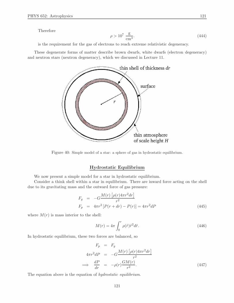
PHYS 652: Astrophysics 121
Thereforeρ > 107
g
cm3. (444)
is the requirement for the gas of electrons to reach extreme relativistic degeneracy.
These degenerate forms of matter describe brown dwarfs, white dwarfs (electron degeneracy)and neutron stars (neutron degeneracy), which we discussed in Lecture 11.
Figure 40: Simple model of a star: a sphere of gas in hydrostatic equilibrium.
Hydrostatic Equilibrium
We now present a simple model for a star in hydrostatic equilibrium.Consider a think shell within a star in equilibrium. There are inward force acting on the shell
due to its gravitating mass and the outward force of gas pressure:
Fg = −GM(r)
[
ρ(r)4πr2dr]
r2
Fp = 4πr2 [P (r + dr)− P (r)] = 4πr2dP (445)
where M(r) is mass interior to the shell:
M(r) = 4π
∫ r
0ρ(r)r2dr. (446)
In hydrostatic equilibrium, these two forces are balanced, so
Fp = Fg
4πr2dP = −GM(r)
[
ρ(r)4πr2dr]
r2
=⇒ dP
dr= −ρ(r)
GM(r)
r2. (447)
The equation above is the equation of hydrostatic equilibrium.
121
PHYS 652: Astrophysics 122
Isothermal Atmospheres in Hydrostatic Equilibrium
Stellar atmospheres are usually thin when compared to the stellar radius, which allows us toapproximate the force due to gravity as a constant throughout the atmosphere:
g ≡ GM
R2≈ const. (448)
Let h be the height of the atmosphere (r-derivative can be replaced with an h-derivative). Thenthe equation of hydrostatic equilibrium [eq. (447)] then becomes
dP
dh= −ρg. (449)
But from the equation of state for ideal gas [eq. 437]:
P =ρkT
µmH=⇒ ρ =
µmH
kTP, (450)
so the eq. (449) becomesdP
dh= − µmHg
kTP. (451)
If we define the “e-folding height” (“scale height”) of the atmosphere as
H ≡ kT
µmHg, (452)
and define the initial condition P (0) = P0, we can rewrite the eq. (449) and integrate it to obtain
dP
dh= −P
H=⇒ dP
P= −dh
H
logP = − h
H+ c =⇒ P (h) = Ce−h/H but P (0) = P0
=⇒ P (h) = P0e−h/H . (453)
Important point: the equation of hydrostatic equilibrium must be accompanied by an equationof state.
Polytropes
Polytropes are a family of equations of state for which the pressure P is given as a power ofdensity ρ. A gas governed by a polytropic process has the equation of state
PV γ = const. (454)
Since ρ = M/V , where M is the mass of gas contained in volume V , we have
P ∝ V −γ ∝(
M
ρ
)−γ,
=⇒ P = κργ , κ = const. (455)
Gas obeying an equation of state of this form is called a polytrope. Examples of polytropes aregiven in Table 7.
122
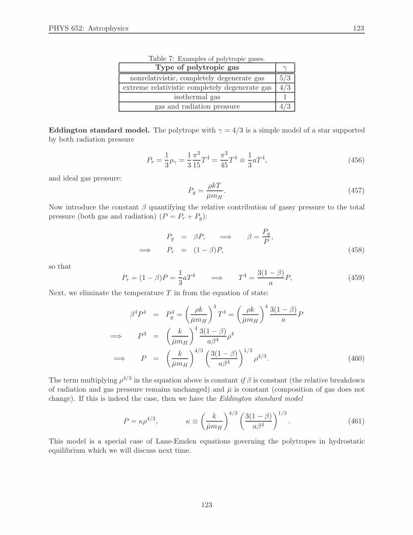
PHYS 652: Astrophysics 123
Table 7: Examples of polytropic gases.
Type of polytropic gas γ
nonrelativistic, completely degenerate gas 5/3
extreme relativistic completely degenerate gas 4/3
isothermal gas 1
gas and radiation pressure 4/3
Eddington standard model. The polytrope with γ = 4/3 is a simple model of a star supportedby both radiation pressure
Pr =1
3ργ =
1
3
π2
15T 4 =
π2
45T 4 ≡ 1
3aT 4, (456)
and ideal gas pressure:
Pg =ρkT
µmH. (457)
Now introduce the constant β quantifying the relative contribution of gassy pressure to the totalpressure (both gas and radiation) (P = Pr + Pg):
Pg = βP, =⇒ β =PgP
,
=⇒ Pr = (1− β)P, (458)
so that
Pr = (1− β)P =1
3aT 4 =⇒ T 4 =
3(1 − β)
aP, (459)
Next, we eliminate the temperature T in from the equation of state:
β4P 4 = P 4g =
(
ρk
µmH
)4
T 4 =
(
ρk
µmH
)4 3(1− β)
aP
=⇒ P 3 =
(
k
µmH
)4 3(1 − β)
aβ4ρ4
=⇒ P =
(
k
µmH
)4/3(3(1− β)
aβ4
)1/3
ρ4/3. (460)
The term multiplying ρ4/3 in the equation above is constant if β is constant (the relative breakdownof radiation and gas pressure remains unchanged) and µ is constant (composition of gas does notchange). If this is indeed the case, then we have the Eddington standard model
P = κρ4/3, κ ≡(
k
µmH
)4/3 (3(1− β)
aβ4
)1/3
. (461)
This model is a special case of Lane-Emden equations governing the polytropes in hydrostaticequilibrium which we will discuss next time.
123
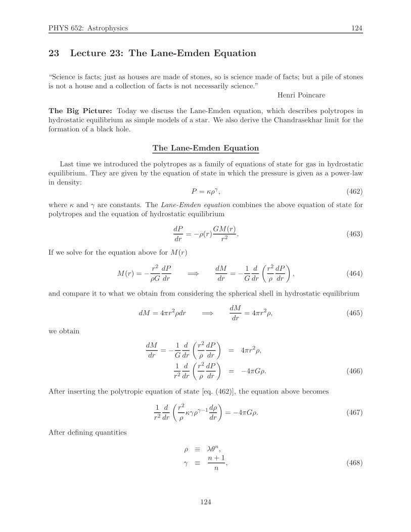
PHYS 652: Astrophysics 124
23 Lecture 23: The Lane-Emden Equation
“Science is facts; just as houses are made of stones, so is science made of facts; but a pile of stonesis not a house and a collection of facts is not necessarily science.”
Henri Poincare
The Big Picture: Today we discuss the Lane-Emden equation, which describes polytropes inhydrostatic equilibrium as simple models of a star. We also derive the Chandrasekhar limit for theformation of a black hole.
The Lane-Emden Equation
Last time we introduced the polytropes as a family of equations of state for gas in hydrostaticequilibrium. They are given by the equation of state in which the pressure is given as a power-lawin density:
P = κργ , (462)
where κ and γ are constants. The Lane-Emden equation combines the above equation of state forpolytropes and the equation of hydrostatic equilibrium
dP
dr= −ρ(r)
GM(r)
r2. (463)
If we solve for the equation above for M(r)
M(r) = − r2
ρG
dP
dr=⇒ dM
dr= − 1
G
d
dr
(
r2
ρ
dP
dr
)
, (464)
and compare it to what we obtain from considering the spherical shell in hydrostatic equilibrium
dM = 4πr2ρdr =⇒ dM
dr= 4πr2ρ, (465)
we obtain
dM
dr= − 1
G
d
dr
(
r2
ρ
dP
dr
)
= 4πr2ρ,
1
r2d
dr
(
r2
ρ
dP
dr
)
= −4πGρ. (466)
After inserting the polytropic equation of state [eq. (462)], the equation above becomes
1
r2d
dr
(
r2
ρκγργ−1 dρ
dr
)
= −4πGρ. (467)
After defining quantities
ρ ≡ λθn,
γ ≡ n+ 1
n, (468)
124
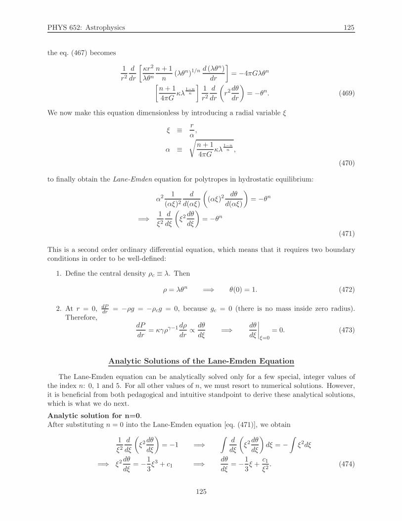
PHYS 652: Astrophysics 125
the eq. (467) becomes
1
r2d
dr
[
κr2
λθnn+ 1
n(λθn)1/n
d (λθn)
dr
]
= −4πGλθn
[
n+ 1
4πGκλ
1−nn
]
1
r2d
dr
(
r2dθ
dr
)
= −θn. (469)
We now make this equation dimensionless by introducing a radial variable ξ
ξ ≡ r
α,
α ≡√
n+ 1
4πGκλ
1−nn ,
(470)
to finally obtain the Lane-Emden equation for polytropes in hydrostatic equilibrium:
α2 1
(αξ)2d
d(αξ)
(
(αξ)2dθ
d(αξ)
)
= −θn
=⇒ 1
ξ2d
dξ
(
ξ2dθ
dξ
)
= −θn
(471)
This is a second order ordinary differential equation, which means that it requires two boundaryconditions in order to be well-defined:
1. Define the central density ρc ≡ λ. Then
ρ = λθn =⇒ θ(0) = 1. (472)
2. At r = 0, dPdr = −ρg = −ρcg = 0, because gc = 0 (there is no mass inside zero radius).
Therefore,dP
dr= κγργ−1 dρ
dr∝ dθ
dξ=⇒ dθ
dξ
∣
∣
∣
∣
ξ=0
= 0. (473)
Analytic Solutions of the Lane-Emden Equation
The Lane-Emden equation can be analytically solved only for a few special, integer values ofthe index n: 0, 1 and 5. For all other values of n, we must resort to numerical solutions. However,it is beneficial from both pedagogical and intuitive standpoint to derive these analytical solutions,which is what we do next.
Analytic solution for n=0.After substituting n = 0 into the Lane-Emden equation [eq. (471)], we obtain
1
ξ2d
dξ
(
ξ2dθ
dξ
)
= −1 =⇒∫
d
dξ
(
ξ2dθ
dξ
)
dξ = −∫
ξ2dξ
=⇒ ξ2dθ
dξ= −1
3ξ3 + c1 =⇒ dθ
dξ= −1
3ξ +
c1ξ2
. (474)
125
PHYS 652: Astrophysics 126
But, using the boundary conditions, we obtain
dθ
dξ
∣
∣
∣
∣
ξ=0
= 0 =⇒ c1 = 0 =⇒ dθ
dξ= −1
3ξ =⇒ θ = −1
6ξ2 + c2
=⇒ θ(0) = 1 =⇒ c2 = 1 =⇒ θ0 = 1− 1
6ξ2. (475)
From the equation above, we see that this configuration has a boundary at ξ =√6, where θ0 → 0.
Analytic solution for n=1.After substituting n = 1 into the Lane-Emden equation [eq. (471)], we obtain
1
ξ2d
dξ
(
ξ2dθ
dξ
)
= −θ =⇒ d
dξ
(
ξ2dθ
dξ
)
= −ξ2θ. (476)
Introduce the variable χ
χ(ξ) ≡ ξθ(ξ) =⇒ θ ≡ χ
ξ. (477)
Thendθ
dξ=
d
dξ
(
χ
ξ
)
=ξχ′ − χ
ξ2, (478)
and the Lane-Emden equation in eq. (476) becomes
d
dξ
(
ξ2dθ
dξ
)
=d
dξ
(
ξχ′) = χ′ + ξχ′′ − χ′ = ξχ′′
=⇒ ξχ′′
ξ2= −χ
ξ=⇒ χ′′ = −χ =⇒ χ′′ + χ = 0. (479)
This is a harmonic oscillator with general solutions
χ(ξ) = A sin ξ +B cos ξ, (480)
or, in terms of θ ≡ χ/ξ
θ(ξ) = Asin ξ
ξ+B
cos ξ
ξ, (481)
After imposing the first boundary condition, the general solution is obtained:
θ(0) = 1 =⇒ B = 0, because limξ→0
cos ξ
ξ= ∞
A = 1, because limξ→0
sin ξ
ξ= 1.
=⇒ θ1(ξ) =sin ξ
ξ. (482)
The second boundary condition dθdξ
∣
∣
∣
ξ=0= 0 is explicitly satisfied, because, after applying L’Hospital’s
rule
limξ→0
ξ cos ξ − sin ξ
ξ2= lim
ξ→0
−ξ sin ξ + cos ξ − cos ξ
2ξ= −1
2limξ→0
sin ξ = 0, (483)
as required. From the eq. (482) above, we see that this configuration is has a boundary at ξ = π,where θ1 → 0.
126
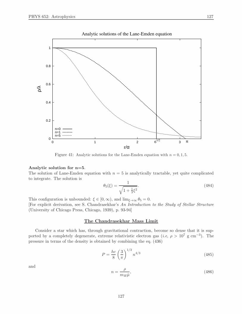
PHYS 652: Astrophysics 127
0
0.2
0.4
0.6
0.8
1
3210
ρ/λ
r/α
Analytic solutions of the Lane-Emden equation
61/2 π
n=0n=1n=5
Figure 41: Analytic solutions for the Lane-Emden equation with n = 0, 1, 5.
Analytic solution for n=5.The solution of Lane-Emden equation with n = 5 is analytically tractable, yet quite complicatedto integrate. The solution is
θ5(ξ) =1
√
1 + 13ξ
2. (484)
This configuration is unbounded: ξ ∈ [0,∞), and limξ→∞ θ5 = 0.[For explicit derivation, see S. Chandrasekhar’s An Introduction to the Study of Stellar Structure(University of Chicago Press, Chicago, 1939), p. 93-94]
The Chandrasekhar Mass Limit
Consider a star which has, through gravitational contraction, become so dense that it is sup-ported by a completely degenerate, extreme relativistic electron gas (i.e, ρ > 107 g cm−3). Thepressure in terms of the density is obtained by combining the eq. (436)
P =hc
8
(
3
π
)1/3
n4/3 (485)
andn =
ρ
mH µ, (486)
127
PHYS 652: Astrophysics 128
to obtain
P =hc
8
(
3
π
)1/3( ρ
mH µe
)4/3
=
(
6.63 × 10⁻²⁷ erg s) (
3× 10¹⁰ cms
)
8
(
3
π
)1/3 1
(1.67 × 10⁻²⁴ g)4/3
(
ρ
µe
)4/3
=⇒ P = 1.24 × 10¹⁵(
ρ
µe
)4/3
, (487)
which is an equation of state for a polytrope with γ = 4/3 and κ = 1.24×10¹⁵
µ4/3e
. Corresponding value
of the index n = 1γ−1 is n = 3.
The mass corresponding to this polytropic configuration can be computed as follows:
M3 =
∫ rmax
0ρ(r)d3r = 4π
∫ rmax
0λρ(r)r2dr = 4π
∫ ξmax
0λθ3(αξ)3d(αξ)
= 4πλα3
∫ ξmax
0
[
− d
dξ
(
ξ2dθ
dξ
)]
dξ
= 4πλα3
[
−ξ2dθ
dξ
]
ξmax
, (488)
where we have used the Lane-Emden equation in eq. (471). The constant λ is defined in eq. (470),and for n = 3 is
α =
√
n+ 1
4πGκλ
1−nn =⇒ α =
√
κ
πGκλ
−23
=⇒ λα3 = λ[ κ
πGλ
−23
]3/2=[ κ
πG
]3/2. (489)
The term in brackets can be evaluated numerically (Table 4.2 of Astrophysics I: Stars by Bowers& Deeming) to about 2.02, so the total mass is
M3 = 4π
1.24×10¹⁵
µ4/3e
π(6.67 × 10⁻⁸)
3/2
2.02 = 4π
[
1.24× 10¹⁵
π(6.67 × 10⁻⁸)
]3/22.02
µ2e
=1.16 × 1034
µ2e
g =1.16 × 1034
µ2e
M⊙1.99 × 1033
=⇒ M3 =5.81
µ2e
M⊙. (490)
Let us now compute µe for a star with relativistic matter degeneracy. In such a star, it is convenientto define the matter density, due essentially to the ions, as ρ = mHµene. Also, let us considercontribution from hydrogen (subscript H), helium (He) and elements with atomic weight greaterthen 4 (Z). Then, from the definition in eq. (439), we have
1
µe=
∑
i
mH
menei =
mH
me
∑
i
nei =mH
me
[
ρeHρ
+ρeHe
ρ+
ρeZρ
]
=mHnH
ρ+
2 mHmHe
mHenHe
ρ+
A2mHmZ
mZnZ
ρ=
ρHρ
+2
4
ρHe
ρ+
A
2A
ρZρ
≡ X +1
2Y +
1
2Z. (491)
128
PHYS 652: Astrophysics 129
Also, conservation of mass imposes that
X + Y + Z = 1 =⇒ Z = 1−X − Y (492)
so
1
µe= X +
1
2Y +
1
2(1−X − Y ) =
1
2X +
1
2=
1 +X
2
=⇒ 1
µe=
1 +X
2=⇒ µe =
2
1 +X. (493)
The stars that are undergoing extreme relativistic degeneracy of matter are highly evolved (nearthe end of their life-cycle), which means that it is reasonable to assume that most of their hydrogenfuel has been burned up, so
X ≈ 0 =⇒ µe ≈ 2. (494)
Finally, we combine this result with the eq. (490) to obtain the Chandrasekhar mass limit:
MCh =5.81
µ2e
M⊙ =5.81
22M⊙ =⇒ MCh = 1.45M⊙. (495)
When a star runs out of fuel, it will explode into a supernova or a helium flash (see Fig. 16). TheSchwarzschild mass limit implies that star remnants with mass M > MCh cannot be supported byelectron degeneracy and therefore will collapse further into a neutron star or a black hole.
129
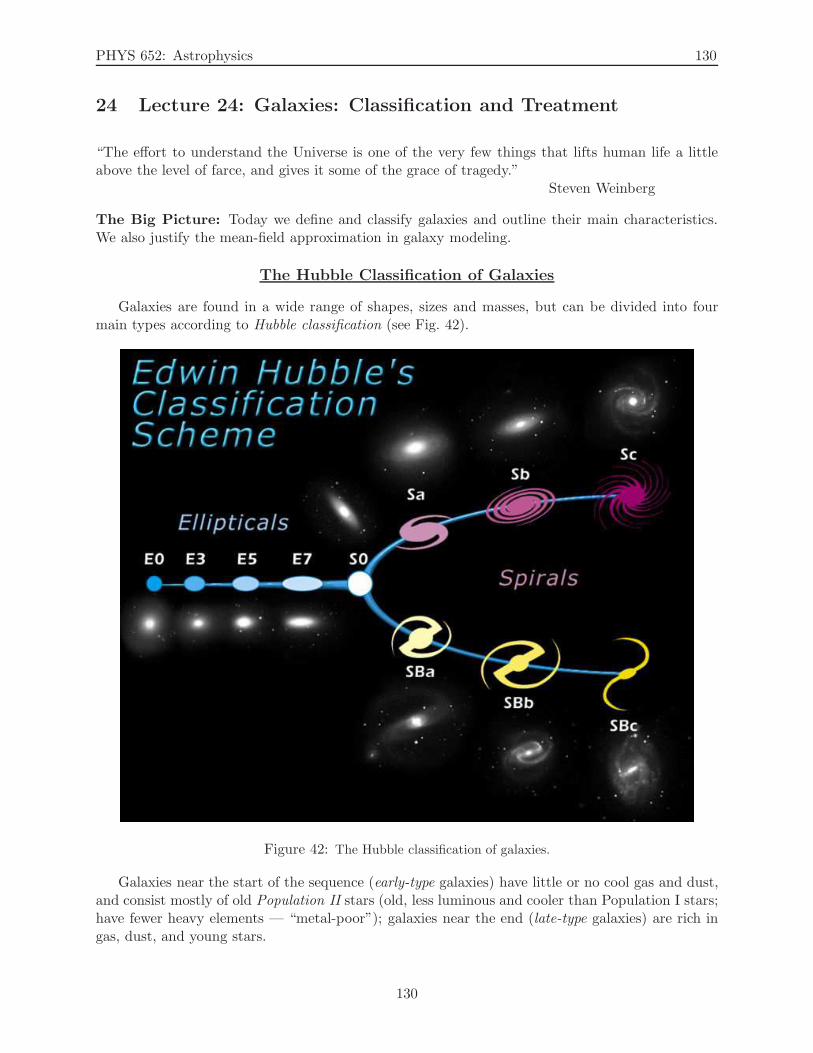
PHYS 652: Astrophysics 130
24 Lecture 24: Galaxies: Classification and Treatment
“The effort to understand the Universe is one of the very few things that lifts human life a littleabove the level of farce, and gives it some of the grace of tragedy.”
Steven Weinberg
The Big Picture: Today we define and classify galaxies and outline their main characteristics.We also justify the mean-field approximation in galaxy modeling.
The Hubble Classification of Galaxies
Galaxies are found in a wide range of shapes, sizes and masses, but can be divided into fourmain types according to Hubble classification (see Fig. 42).
Figure 42: The Hubble classification of galaxies.
Galaxies near the start of the sequence (early-type galaxies) have little or no cool gas and dust,and consist mostly of old Population II stars (old, less luminous and cooler than Population I stars;have fewer heavy elements — “metal-poor”); galaxies near the end (late-type galaxies) are rich ingas, dust, and young stars.
130
PHYS 652: Astrophysics 131
Elliptical Galaxies
Elliptical galaxies are smooth, featureless systems containing little or no gas or dust. Thefraction of bright galaxies that are elliptical is a function of the local density, ranging from about10% in low-density regions to 40% in dense clusters of galaxies. The isophotes (contours of constantsurface brightness) are approximately concentric ellipses, with axis ratio b/a ranging from 1 to about0.3. Elliptical galaxies are denoted by the symbols E0, E1, etc., where the brightest isophotes of agalaxy of type En have axis ratio b/a = 1 − n/10. The ellipticity is ǫ = 1 − b/a. Thus the mostelongated elliptical galaxies are of type E7. Since we see only the projected brightness distribution,it is impossible to determine directly whether elliptical galaxies are axisymmetric or triaxial.
Surface brightness profiles.The surface brightness of an elliptical galaxy falls off smoothly with radius. Often the outermostparts of a galaxy are undetectable against the background night-sky brightness. The surface-brightness profiles of most elliptical galaxies can be fit reasonably well by the empirically-motivatedR1/4 or de Vaucouleurs’ law
I(R) = I(0)e−kR1/4
, (496)
where the effective radius Re is the radius of the isophote containing half of total luminosity andIe is the surface brightness Re. The effective radius is typically 3/h kpc for bright ellipticals and issmaller for fainter galaxies.
However, it has been shown that de Vaucouleurs’ R1/4 law is appropriate only for a subsetof elliptical galaxies. Generalizing de Vaucouleurs’ law to allow for a varying rate of exponentialdecay, we arrive at the Sersic law (of which de Vaucouleurs’ is a special case when n = 4):
I(R) = I(0)e−kR1/n
. (497)
It has been shown that there exists a strong correlation between the observed size of the ellipticalgalaxy and the best-fit index n: heavier elliptical galaxies have higher values of n.
Central density cusps and supermassive black holes.With the advent of the Hubble Space Telescope, modeling of elliptical galaxies has undergone arevolution: elliptical galaxies are not well-approximated by density profiles with central cores, asonce thought, but have logarithmic slopes of the density profiles which increase all the way tothe smallest observable radius: the elliptical galaxies have central density cusps. Furthermore,the centers of most elliptical galaxies harbor a supermassive black hole, with mass millions (andsometimes billions) times that of our Sun.
No net rotation.Most giant elliptical galaxies exhibit little or no rotation, even those with highly elongated isophotes.Their stars have random velocities along the line of sight whose root mean square dispersion σp canbe measured from the Doppler broadening of spectral lines. The velocity dispersion in the innerfew kiloparsecs is correlated with luminosity according to the Faber-Jackson law
σp ≃ 220(L/L⋆)1/4 km s−1. (498)
Lenticular Galaxies
Lenticular galaxies have a prominent disk that contains no gas, bright young stars, or spiralarms. Lenticular disks are smooth and featureless, like elliptical galaxies, but obey the exponential
131
PHYS 652: Astrophysics 132
surface-brightness law characteristic of spiral galaxies:
I(R) = I(0)e−R/Rd , (499)
where the disc scale length Rd = 3.5 ± 0.5 kpc. Lenticulars are labeled by the notation S0 inHubble’s classification scheme. They are very rare in low-density regions, comprising less then 10%of all bright galaxies, but up to half of all galaxies in high-density regions are S0’s.
The lenticulars form a transition class between elliptical and spirals. The transition is smoothand continuous, so that there are S0 galaxies that might well be classified as E7, and others thatsometimes been classified as spirals.
The strong dependence of the fractional abundance of the fractional abundance of S0 galaxieson the local density is obviously an important — but still controversial — clue to the mechanismof galaxy formation.
Spiral Galaxies
Spiral galaxies, like the Milky Way, contain a prominent disk composed of gas, dust and Popu-lation I stars (Population I stars include the Sun and tend to be luminous, hot and young, concen-trated in the disks of spiral galaxies, and particularly found in the spiral arms). In all these systemsthe disk contains spiral arms, filaments of bright stars, gas, and dust, in which large numbers ofstars are currently forming. The spiral arms vary greatly in their length and prominence from onespiral galaxy to another but are almost always present.
In low-density regions of the Universe, almost 80% of all bright galaxies are spirals, but thefraction drops to 10% in dense regions such as cluster cores.
The distribution of surface brightness in spiral galaxy disks obeys the exponential law. Thetypical disk scale length is Rd ≃ 3/h kpc, and the central surface brightness is remarkably constantat I0 ≃ 140L⊙ pc−2.
The circular-speed curves of most spiral galaxies are nearly flat, vc(R) independent of R, exceptnear the center, where the circular speed drops to zero. Typical circular speeds are between 200and 300 km s−1. It is a remarkable fact that the circular speed curves still remain flat even at radiiwell beyond the outer edge of the visible galaxy, thus implying the presence of invisible or darkmass in the outer parts of the galaxy.
Spiral galaxies also contain a spheroid of Population II stars. The luminosity of the spheroidrelative to the disk correlates well with a number of other properties of the galaxy, in particularthe fraction of the disk mass in gas, the color of the disk, and how tightly the spiral arms arewound. This correlation is the basis of Hubble’s classification of spiral galaxies. Hubble dividedspiral galaxies into a sequence of four classes or types, called Sa, Sb, Sc, Sd. Along the sequenceSa → Sd the relative luminosity of the spheroid decreases, the relative mass of gas increases, andthe spiral arms become more loosely wound. The spiral arms also become more clumpy, so thatindividual patches of young stars and HII regions (a cloud of glowing gas and plasma, sometimesseveral hundred light-years across, in which star formation is taking place) become visible. Ourgalaxy appears to be intermediate between Sb and Sc, so its Hubble type is written as Sbc.
Irregular Galaxies
Any classification scheme has to contain an attic – a class into which objects that conform tono particular pattern can be placed. Since the time of Hubble, nonconformist galaxies have beendumped into the irregular class (denoted Irr). A minority of Irr galaxies are spiral or ellipticalgalaxies that have been violently distorted by a recent encounter with a neighbor. However, the
132
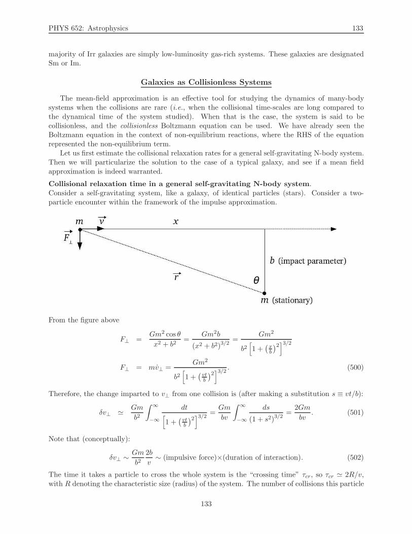
PHYS 652: Astrophysics 133
majority of Irr galaxies are simply low-luminosity gas-rich systems. These galaxies are designatedSm or Im.
Galaxies as Collisionless Systems
The mean-field approximation is an effective tool for studying the dynamics of many-bodysystems when the collisions are rare (i.e., when the collisional time-scales are long compared tothe dynamical time of the system studied). When that is the case, the system is said to becollisionless, and the collisionless Boltzmann equation can be used. We have already seen theBoltzmann equation in the context of non-equilibrium reactions, where the RHS of the equationrepresented the non-equilibrium term.
Let us first estimate the collisional relaxation rates for a general self-gravitating N-body system.Then we will particularize the solution to the case of a typical galaxy, and see if a mean fieldapproximation is indeed warranted.
Collisional relaxation time in a general self-gravitating N-body system.Consider a self-gravitating system, like a galaxy, of identical particles (stars). Consider a two-particle encounter within the framework of the impulse approximation.
From the figure above
F⊥ =Gm2 cos θ
x2 + b2=
Gm2b
(x2 + b2)3/2=
Gm2
b2[
1 +(
xb
)2]3/2
F⊥ = mv⊥ =Gm2
b2[
1 +(
vtb
)2]3/2
. (500)
Therefore, the change imparted to v⊥ from one collision is (after making a substitution s ≡ vt/b):
δv⊥ ≃ Gm
b2
∫ ∞
−∞
dt[
1 +(
vtb
)2]3/2
=Gm
bv
∫ ∞
−∞
ds
(1 + s2)3/2=
2Gm
bv. (501)
Note that (conceptually):
δv⊥ ∼ Gm
b22b
v∼ (impulsive force)×(duration of interaction). (502)
The time it takes a particle to cross the whole system is the “crossing time” τcr, so τcr ≃ 2R/v,with R denoting the characteristic size (radius) of the system. The number of collisions this particle
133
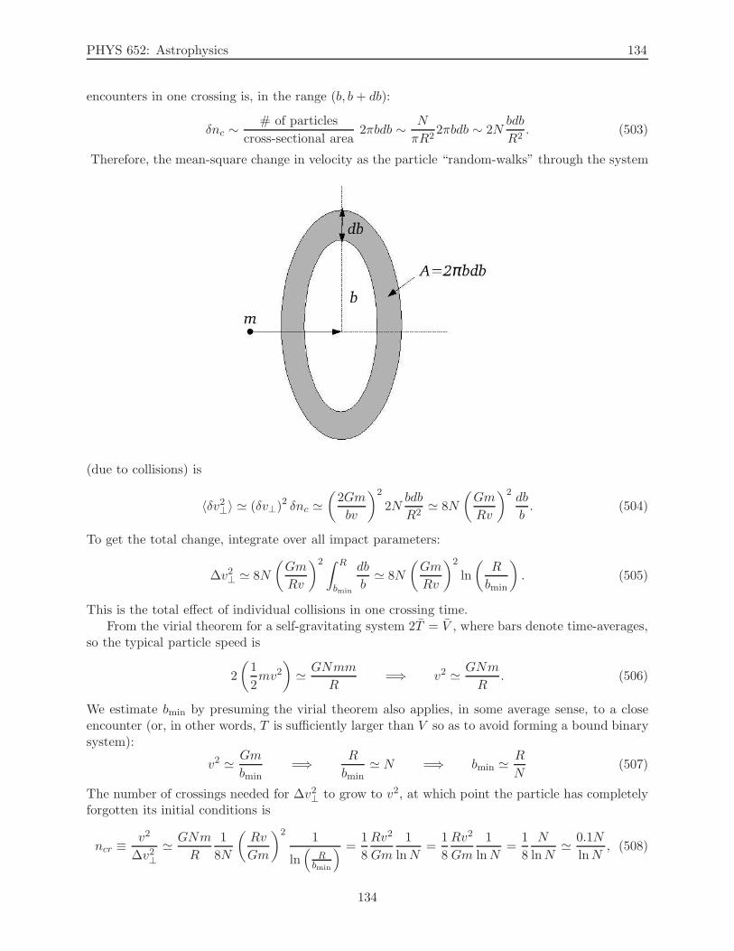
PHYS 652: Astrophysics 134
encounters in one crossing is, in the range (b, b+ db):
δnc ∼# of particles
cross-sectional area2πbdb ∼ N
πR22πbdb ∼ 2N
bdb
R2. (503)
Therefore, the mean-square change in velocity as the particle “random-walks” through the system
(due to collisions) is
〈δv2⊥〉 ≃ (δv⊥)2 δnc ≃
(
2Gm
bv
)2
2Nbdb
R2≃ 8N
(
Gm
Rv
)2 db
b. (504)
To get the total change, integrate over all impact parameters:
∆v2⊥ ≃ 8N
(
Gm
Rv
)2 ∫ R
bmin
db
b≃ 8N
(
Gm
Rv
)2
ln
(
R
bmin
)
. (505)
This is the total effect of individual collisions in one crossing time.From the virial theorem for a self-gravitating system 2T = V , where bars denote time-averages,
so the typical particle speed is
2
(
1
2mv2
)
≃ GNmm
R=⇒ v2 ≃ GNm
R. (506)
We estimate bmin by presuming the virial theorem also applies, in some average sense, to a closeencounter (or, in other words, T is sufficiently larger than V so as to avoid forming a bound binarysystem):
v2 ≃ Gm
bmin=⇒ R
bmin≃ N =⇒ bmin ≃ R
N(507)
The number of crossings needed for ∆v2⊥ to grow to v2, at which point the particle has completelyforgotten its initial conditions is
ncr ≡v2
∆v2⊥≃ GNm
R
1
8N
(
Rv
Gm
)2 1
ln(
Rbmin
) =1
8
Rv2
Gm
1
lnN=
1
8
Rv2
Gm
1
lnN=
1
8
N
lnN≃ 0.1N
lnN, (508)
134
PHYS 652: Astrophysics 135
and the corresponding relaxation time is
τR = ncrτcr ≃0.1N
lnNτcr ≫ τcr. (509)
Let us now estimate the crossing time for the self-gravitating system τcr. Consider a particlefreely-falling along a diameter of a uniform-density sphere:
r = −GM(r)
r2= −G
(
4π3 r3ρ
)
r2= −
(
4πG
3ρ
)
r
r +
(
4πG
3ρ
)
r = 0 =⇒ r + ω2r = 0
ω2 =4π
3Gρ =
(
2π
2τcr
)2
=⇒ τcr =
√
3π
4Gρ
=⇒ τcr ≃ 1√Gρ
(510)
Therefore, estimated collisional relaxation time for a typical self-gravitating N-body system is
τR ≃ 0.1N
lnN
1√Gρ
. (511)
Collisional relaxation time for a typical elliptical galaxy.A typical elliptical galaxy contains about 1012 stars of typical mass of M⊙, and has a radius ofabout R ≈ 100 kpc, so
N ≃ 1012,
R ≃ 100 kpc ≃ 105(3.26) light − years ≃ 105 (3.26)(
3× 10⁸ ms−1)
(π × 107 s)
≃ 3× 10²¹ m
m ≃ M⊙ ≃ 2× 1030 kg,
=⇒ τR ≃ 0.1
ln (1012)
(
1012(
3× 10²¹)3
(6.7× 10⁻¹¹) (2× 1030)
)1/2
≃ 5× 1025s ≃ 5× 1025
3× 10⁷years
=⇒ τR ≃ 1018 years ∼ 108tHubble. (512)
The relaxation time due to collisions is orders of magnitude longer than the age of the Universe,which means that galaxies are well-approximated by collisionless, mean-field approximation andthe collisionless Boltzmann equation.
135
PHYS 652: Astrophysics 136
25 Lecture 25: Galaxies: Analytic Models
“Science is simply common sense at its best that is, rigidly accurate in observation, and mercilessto fallacy in logic.”
Thomas Henry Huxley
The Big Picture: Last time we showed that individual stellar encounters are unimportant in thedynamics of the galaxy, which justifies the mean-field approximation and the use of the collision-less Boltzmann equation. Today we derive the collisionless Boltzmann equation in the context ofgalaxies, formulate the self-consistent problem and outline a few analytic approaches to solving it.
The study of galactic systems — the dynamics, kinematics, morphology — is a major tool incomprehending some of the key issues in astrophysics relating to the origin, evolution and structureof the Universe.
In modeling of galactic systems, we move from the simplest approximations to galaxy shapes(spherical — 1 dof) to more general (axisymmetric — 2 dof; and triaxial — 3 dof). However, wefirst must establish which equations govern the dynamics of galactic systems.
The Collisionless Boltzmann Equation
Earlier, we have demonstrated that in galaxies the stellar encounters are unimportant; in otherwords, the mean-free path between collisions is considerably (orders of magnitude!) longer than theage of the Universe. This justifies the collisionless approximation and the use of the collisionlessBoltzmann equation (also known as the Vlasov equation).
Imagine a large number of stars moving under the influence of a smooth potential Φ(x, t). Atany time t, a full description of the state of any collisionless system is given by specifying the numberof stars f(x,v, t)d3xd3v having positions in the small volume d3x centered on x and velocities inthe small range d3v centered on v. The quantity f(x,v, t) is called the distribution function orphase-space density of the system. Clearly f ≥ 0 everywhere.
If we know the initial coordinates and velocities of every star, Newton’s laws enable us toevaluate their positions and velocities at any later time. Thus, given f(x,v, t0), it should bepossible to calculate f(x,v, t) for any t using only the information that is contained in f(x,v, t0).Now, consider the flow of points in phase space that arises as stars move along their orbits. Thecoordinates in phase-space are
(x,v) ≡ w ≡ (w1, ..., w6), (513)
so that the velocity of this flow can be written as
w = (x, v) = (x,−∇Φ), (514)
where we have used from the Hamiltonian formulation v = −∇Φ.A characteristic of the flow described by w is that it conserves stars: in the absence of encounters
stars do not jump from one point in phase-space to another, but rather drift smoothly throughspace. Therefore, the density of stars f(w, t) satisfies a continuity equation analogous to thatsatisfied by the density ρ(x, t) of the ordinary fluid flow:
∂f
∂t+
6∑
i=1
∂(fwi)
dwi= 0. (515)
136
PHYS 652: Astrophysics 137
The physical content of this equation can be seen by integrating it over some volume of phasespace. The first term then describes the rate at which the collection of stars inside this volume isincreasing, while an application of the divergence theorem shows that the second term describesthe rate at which stars flow out of this volume.
The flow described by w is very special, because it has the property that
6∑
i=1
∂widwi
=
3∑
j=1
∂vjdxj
+∂vjdvj
=
3∑
j=1
− ∂
dvj
(
∂Φ
dxj
)
= 0. (516)
Here (∂vj/∂xj) = 0 because vi and xi are independent coordinates of phase-space, and the laststep follows because ∇Φ does not depend on velocities. If we use eq. (516) to simplify eq. (515),we obtain the collisionless Boltzmann equation (also known as the Vlasov equation):
∂f
∂t+
6∑
i=1
∂(fwi)
∂wi= 0
∂f
∂t+
6∑
i=1
(
f∂wi∂wi
+ wi∂f
∂wi
)
= 0
∂f
∂t+
3∑
i=1
(
xi∂f
∂xi+ vi
∂f
∂vi
)
= 0
∂f
∂t+
3∑
i=1
(
vi∂f
∂xi− ∂Φ
∂xi
∂f
∂vi
)
= 0 (517)
or, in vector notation∂f
∂t+ v · ∇f −∇Φ · ∂f
∂v= 0. (518)
Equation (518) is the fundamental equation of stellar dynamics.The meaning of the collisionless Boltzmann equation can be clarified by extending to six diver-
sions the concept of the convective derivative. We define
df
dt≡ ∂f
∂t+
6∑
i=1
wi∂f
∂wi. (519)
df/dt represents the rate of change of density of phase points as seen by an observer who movesthrough phase-space with a star at velocity w. The collisionless Boltzmann equation is then simply
df
dt= 0. (520)
In words, the flow of stellar phase points through phase-space is incompressible; the phase-spacedensity f around the phase point of a given star always remains the same.
The Self-Consistent Problem
The collisionless Boltzmann equation does not provide the closed system of equation. In orderto have a closed system of equation, we must have as many equations as we have quantities. Here,it means that we must relate Φ and f . The Poisson equation
∆Φ(x, t) = 4πGρ(x, t) (521)
137
PHYS 652: Astrophysics 138
relates the mass-density ρ(x, t) to the distribution function f(x,v, t). Finally, the potential Φ(x, t)and density ρ(x, t) are related as
ρ(x, t) =
∫
f(x,v, t)d3v, (522)
which provides the link Φ ↔ ρ ↔ f , and closes the system of equations. Solving the system ofequations:
∂f
∂t+ v · ∇f − ∇Φ · ∂f
∂v= 0,
ρ(x, t) =
∫
f(x,v, t)d3v,
∆Φ(x, t) = 4πGρ(x, t) (523)
simultaneously is called the self-consistent problem.
Integrals of Motion and Jeans Theorem
An integral of motion I(x,v) is any function of the phase-space coordinates (x,v) that isconstant along any orbit:
I[x(t1),v(t1)] = I[x(t2),v(t2)], (524)
ord
dtI[x(t1),v(t1)] = 0 =
∂I
∂x
∂x
∂t+
∂I
∂v
∂v
∂t= v
∂I
∂x−∇Φ
∂I
∂v, (525)
which satisfies the collisionless Boltzmann equation. This leads to the following theorems.
Jeans theorem. Any steady-state solution of the collisionless Boltzmann equation depends on thephase-space coordinates only through integrals of motion in the galactic potential, and any functionof the integrals yields a steady-state solution of the collisionless Boltzmann equation.
Strong Jeans theorem. The DF of a steady-state galaxy in which almost all orbits are regularwith incommensurate frequencies may be presumed to be a function only of the three independentisolating integrals.
In other words, the Jeans theorem tells us that if I1,..., I5 are five independent integrals ofmotion in a given potential, then any DFs of the forms f(I1), f(I1, I2), ..., f(I1, ..., I5) are solutionsof the collisionless Boltzmann equation. The strong Jeans theorem tells us that if the potentialis regular (integrable), for all practical purposes any time-independent galaxy may be representedby a solution of the form f(I1, I2, I3), where I1, I2 and I3 are any three independent integrals ofmotion.
For example, in a spherical system (1 dof), the DF is a function of energy: f(E); in an (in-tegrable) axisymmetric system (2 dof), the DF is a function of energy and a z-component of theangular momentum f(E,Lz); and in a (integrable) triaxial systems (3 dof), the DF is a function ofenergy and two more integrals of motion: f(E, I2, I3). In general, integrals of motion I2 and I3 arenot known, except in very special cases (of limited physical importance). For equilibrium modelsdf/dt = 0, so the energy is conserved, and therefore an integral of motion.
So, how does one construct DFs for galactic models?
Analytic Solutions to the Self-Consistent Problem
138
PHYS 652: Astrophysics 139
The DFs for galactic models can be obtained analytically only for a few special cases. Thesespecial cases are important phenomenologically and pedagogically, as they offer a “peek” into thedynamics of galaxies. However, their physical relevance is limited, because they represent eithersimple 1 dof models (spheres), or density distributions which give poor fits to the observed profiles.
From f to ρ.As a simple spherical model (1 dof), one can start with the predefined DF f(E) and computethe corresponding ρ. This is the most straightforward method. The drawback of this approach,however, is that the properties of the resulting density distribution are not adjustable to fit theobserved profiles.
We start with an assumed form of the DF f , integrate to obtain ρ, and solve the Poissonequation to get the corresponding Φ.
Define relative potential and relative energy, respectively:
Ψ ≡ −Φ+ Φ0,
ǫ ≡ −E +Φ0 = Ψ− 1
2v2, (526)
and assume the DF of the following form:
f(ǫ) =
Fǫn−3/2 ǫ > 0,0 ǫ ≤ 0,
(527)
where F is a constant. Then the mass-density is computed by integrating over velocities [seeeq. (522)]:
ρ(x) =
∫ ∞
0f(ǫ)d3v =
∫ ∞
0f
(
Ψ− 1
24πv2
)
v2dv = 4πF
∫
√2Ψ
0
(
Ψ− 1
2v2)n−3/2
v2dv, (528)
where we have used d3v = 4πv2. After introducing the variable θ, such that v2 = 2Ψcos2 θ, weobtain
ρ(x) = 4πF
∫ π/2
0Ψn−3/2
(
1− cos2 θ)n−3/2 (
2Ψ cos2 θ)
(√2Ψ sin θdθ
)
=
= 8√2πFΨn
∫ π/2
0sin2n−2 θ cos2 θdθ
= 8√2πFΨn
[
∫ π/2
0sin2n−2 θdθ −
∫ π/2
0sin2n θdθ
]
=⇒ ρ(x) = cnΨn, (529)
where
cn =(2π)3/2
(
n− 32
)
!
n!F. (530)
For cn to be finite, n > 1/2.We now solve the Poisson equation by substituting the eqs. (526) and (529) into the eq. (521)
expressed in spherical coordinates:
1
r2d
dr
(
r2dΦ
dr
)
= 4πGρ
− 1
r2d
dr
(
r2dΨ
dr
)
= 4πGcnΨn. (531)
139
PHYS 652: Astrophysics 140
Now let
s ≡ r
b,
ϕ ≡ Ψ
Ψ0,
b ≡ 1√
4πGΨn−10 cn
. (532)
Then we arrive at1
s2d
ds
(
s2dϕ
ds
)
=
−ϕn ϕ > 0,0 ϕ ≤ 0,
(533)
which is the Lane-Emden equation for polytropes! Again, this second-order ODE is to be solvedwith the initial conditions:
1. ϕ(0) = 1 by definition;
2. dϕds
∣
∣
∣
s=0= 0: no gravitational force at the center.
Table 8: Properties of the solutions to the Lane-Emden equation [γ = (n+ 1)/n].
Lane-Emden index n radius mass polytropic index γ
1 ≤ n < 5 finite finite 6/5 < γ ≤ ∞5 ≤ n < ∞ infinite finite 1 < γ ≤ 6/5
n = ∞ infinite infinite γ = 1
One of the popular early simple models for the DF in a spherical galaxy is the solution to theLane-Emden equation with n = 5. It is called the Plummer model:
f(ǫ) = Fǫ7/2,
Φ(r) = − GM√r2 + b2
,
ρ(r) =3Mb2
4π (r2 + b2)5/2. (534)
From ρ to f .Another simple spherical model (1 dof) is obtained by starting with the predefined density ρ(r)and compute the corresponding DF f(E).
We first invert the integral for ρ in terms of f , in order to get f in terms of ρ:
ρ(r) =
∫
√2Ψ(r)
0f(ǫ)4πv2dv ǫ = Ψ(r)− 1
2v2, dǫ = −vdv
ρ(Ψ) = 2π√2
∫ Ψ
ǫ=0f(ǫ)
√Ψ− ǫ dǫ
dρ(Ψ)
dΨ= 4π
√2
∫ Ψ
ǫ=0
f(ǫ)√Ψ− ǫ
dǫ (535)
140
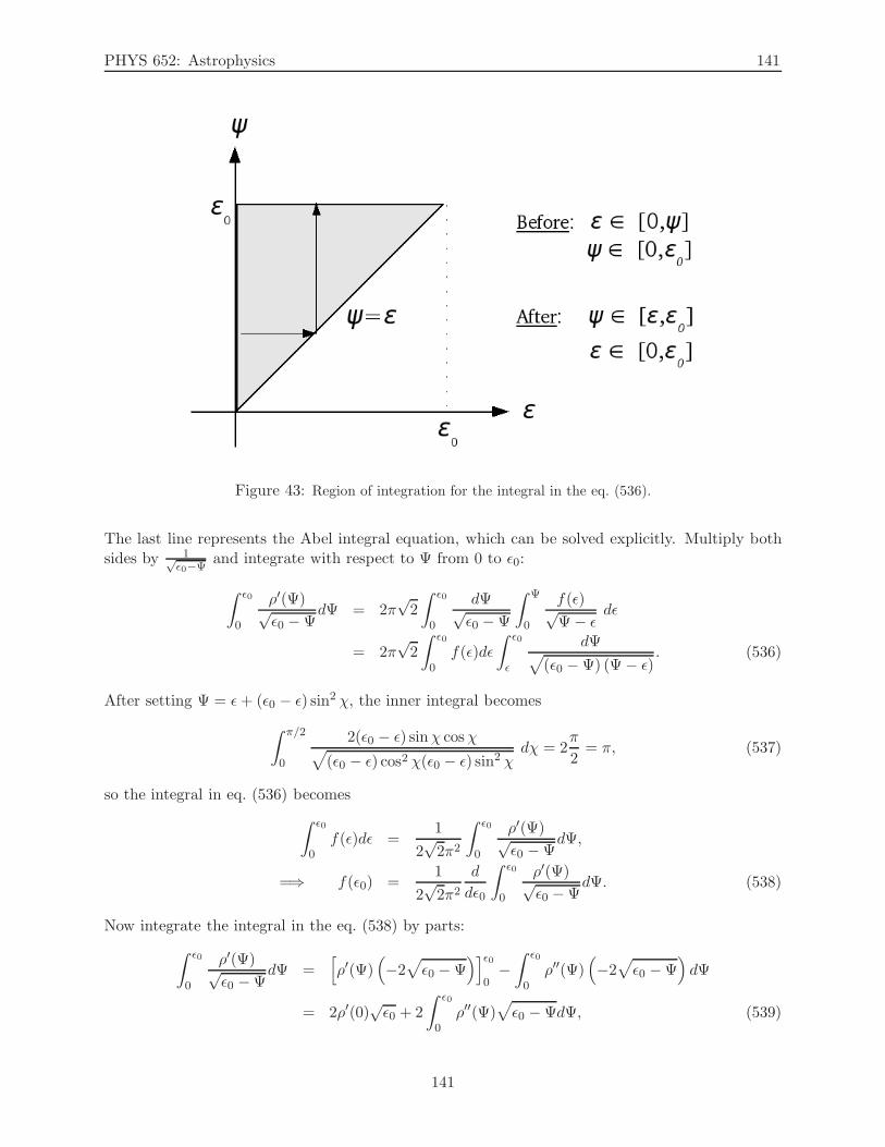
PHYS 652: Astrophysics 141
Figure 43: Region of integration for the integral in the eq. (536).
The last line represents the Abel integral equation, which can be solved explicitly. Multiply bothsides by 1√
ǫ0−Ψand integrate with respect to Ψ from 0 to ǫ0:
∫ ǫ0
0
ρ′(Ψ)√ǫ0 −Ψ
dΨ = 2π√2
∫ ǫ0
0
dΨ√ǫ0 −Ψ
∫ Ψ
0
f(ǫ)√Ψ− ǫ
dǫ
= 2π√2
∫ ǫ0
0f(ǫ)dǫ
∫ ǫ0
ǫ
dΨ√
(ǫ0 −Ψ) (Ψ− ǫ). (536)
After setting Ψ = ǫ+ (ǫ0 − ǫ) sin2 χ, the inner integral becomes
∫ π/2
0
2(ǫ0 − ǫ) sinχ cosχ√
(ǫ0 − ǫ) cos2 χ(ǫ0 − ǫ) sin2 χdχ = 2
π
2= π, (537)
so the integral in eq. (536) becomes
∫ ǫ0
0f(ǫ)dǫ =
1
2√2π2
∫ ǫ0
0
ρ′(Ψ)√ǫ0 −Ψ
dΨ,
=⇒ f(ǫ0) =1
2√2π2
d
dǫ0
∫ ǫ0
0
ρ′(Ψ)√ǫ0 −Ψ
dΨ. (538)
Now integrate the integral in the eq. (538) by parts:
∫ ǫ0
0
ρ′(Ψ)√ǫ0 −Ψ
dΨ =[
ρ′(Ψ)(
−2√
ǫ0 −Ψ)]ǫ0
0−∫ ǫ0
0ρ′′(Ψ)
(
−2√
ǫ0 −Ψ)
dΨ
= 2ρ′(0)√ǫ0 + 2
∫ ǫ0
0ρ′′(Ψ)
√
ǫ0 −ΨdΨ, (539)
141
PHYS 652: Astrophysics 142
so
f(ǫ0) =1
2√2π2
[
ρ′(0)√ǫ0
+
∫ ǫ0
0
ρ′′(Ψ)√ǫ0 −Ψ
dΨ
]
(540)
Equations (538) and (540) are two variants of Eddington’s formula.We now apply Eddington’s formula [top line of eq. (538)] to the density used in the approach
“from f to ρ” ρ(r) = cnΨn:
∫ ǫ0
0f(ǫ)dǫ =
ncn
2√2π2
∫ ǫ0
0
Ψn−1
√ǫ0 −Ψ
dΨ Set t ≡ Ψ
ǫ0
=ncn
2√2π2
∫ 1
0
tn−1ǫn0√ǫ0√1− t
dt
=ncn
2√2π2
ǫn−1/20 β
(
n,1
2
)
=ncn
2√2π2
Γ(n)Γ(
12
)
Γ(
n+ 12
) ǫn−1/20 (541)
because Γ(
12
)
=√π. [Recall Γ(n) = (n− 1)!]. Now differentiate to get
f(ǫ0) =ncn
2√2π2
(
n− 1
2
)
(n− 1)!√π
(
n− 12
)
!ǫn−3/20 =
n!cn
(2π)3/2(
n− 32
)
!ǫn−3/20 = Fǫ
n−3/20 . (542)
Therefore, we recover the DF used in the approach “from f to ρ”, as we should.
Separable (Stackel) potentials.Separable (Stackel) potentials are a spacial family of 3D potentials for which the equations ofmotion separate — and are explicitly known — in ellipsoidal coordinates (λ, µ, ν), defined as theroots of the equation:
x2
τ + α+
y2
τ + β+
z2
τ + γ= 1, (543)
where (x, y, z) are Cartesian coordinates and α, β and γ are constants determining the triaxialshape of the model. We adopt a convention 0 ≤ −γ ≤ ν ≤ −β ≤ µ ≤ −α ≤ λ.
All three integrals of motion have an analytic representation, as well as the density, potentialand the DFs. Orbits in these potentials are combinations of oscillations and rotations in ellipsoidalcoordinates. They are either tubes (along short and long axes) or boxes.
Whereas the separable potentials are not a very good fit to the observed galaxy density profiles(and are therefore of limited use in practice), they provide us with insight into the dynamics oftriaxial systems: the orbits in other, physically more faithful integrable potentials, are generally ofthe same type as in separable potentials. For more on separable potentials, see the seminal paper byde Zeeuw (1985, MNRAS, 216, 273): http://adsabs.harvard.edu/abs/1985MNRAS.216..273D
142
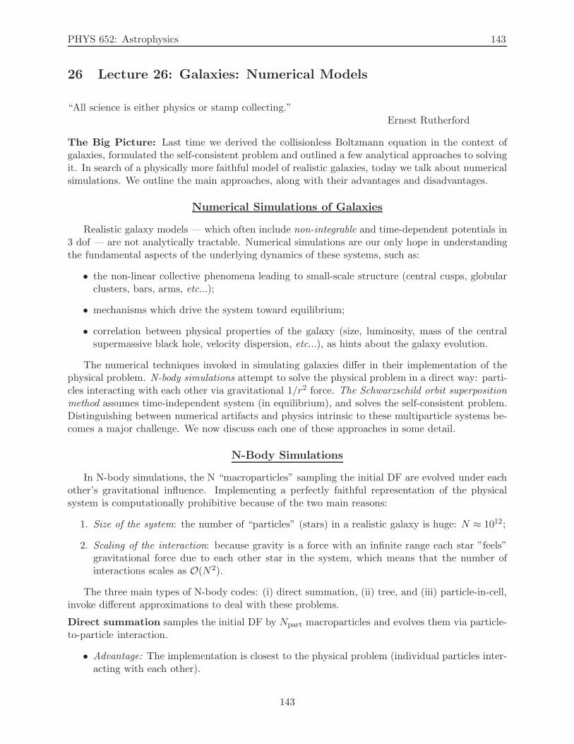
PHYS 652: Astrophysics 143
26 Lecture 26: Galaxies: Numerical Models
“All science is either physics or stamp collecting.”Ernest Rutherford
The Big Picture: Last time we derived the collisionless Boltzmann equation in the context ofgalaxies, formulated the self-consistent problem and outlined a few analytical approaches to solvingit. In search of a physically more faithful model of realistic galaxies, today we talk about numericalsimulations. We outline the main approaches, along with their advantages and disadvantages.
Numerical Simulations of Galaxies
Realistic galaxy models — which often include non-integrable and time-dependent potentials in3 dof — are not analytically tractable. Numerical simulations are our only hope in understandingthe fundamental aspects of the underlying dynamics of these systems, such as:
• the non-linear collective phenomena leading to small-scale structure (central cusps, globularclusters, bars, arms, etc...);
• mechanisms which drive the system toward equilibrium;
• correlation between physical properties of the galaxy (size, luminosity, mass of the centralsupermassive black hole, velocity dispersion, etc...), as hints about the galaxy evolution.
The numerical techniques invoked in simulating galaxies differ in their implementation of thephysical problem. N-body simulations attempt to solve the physical problem in a direct way: parti-cles interacting with each other via gravitational 1/r2 force. The Schwarzschild orbit superpositionmethod assumes time-independent system (in equilibrium), and solves the self-consistent problem.Distinguishing between numerical artifacts and physics intrinsic to these multiparticle systems be-comes a major challenge. We now discuss each one of these approaches in some detail.
N-Body Simulations
In N-body simulations, the N “macroparticles” sampling the initial DF are evolved under eachother’s gravitational influence. Implementing a perfectly faithful representation of the physicalsystem is computationally prohibitive because of the two main reasons:
1. Size of the system: the number of “particles” (stars) in a realistic galaxy is huge: N ≈ 1012;
2. Scaling of the interaction: because gravity is a force with an infinite range each star ”feels”gravitational force due to each other star in the system, which means that the number ofinteractions scales as O(N2).
The three main types of N-body codes: (i) direct summation, (ii) tree, and (iii) particle-in-cell,invoke different approximations to deal with these problems.
Direct summation samples the initial DF by Npart macroparticles and evolves them via particle-to-particle interaction.
• Advantage: The implementation is closest to the physical problem (individual particles inter-acting with each other).
143
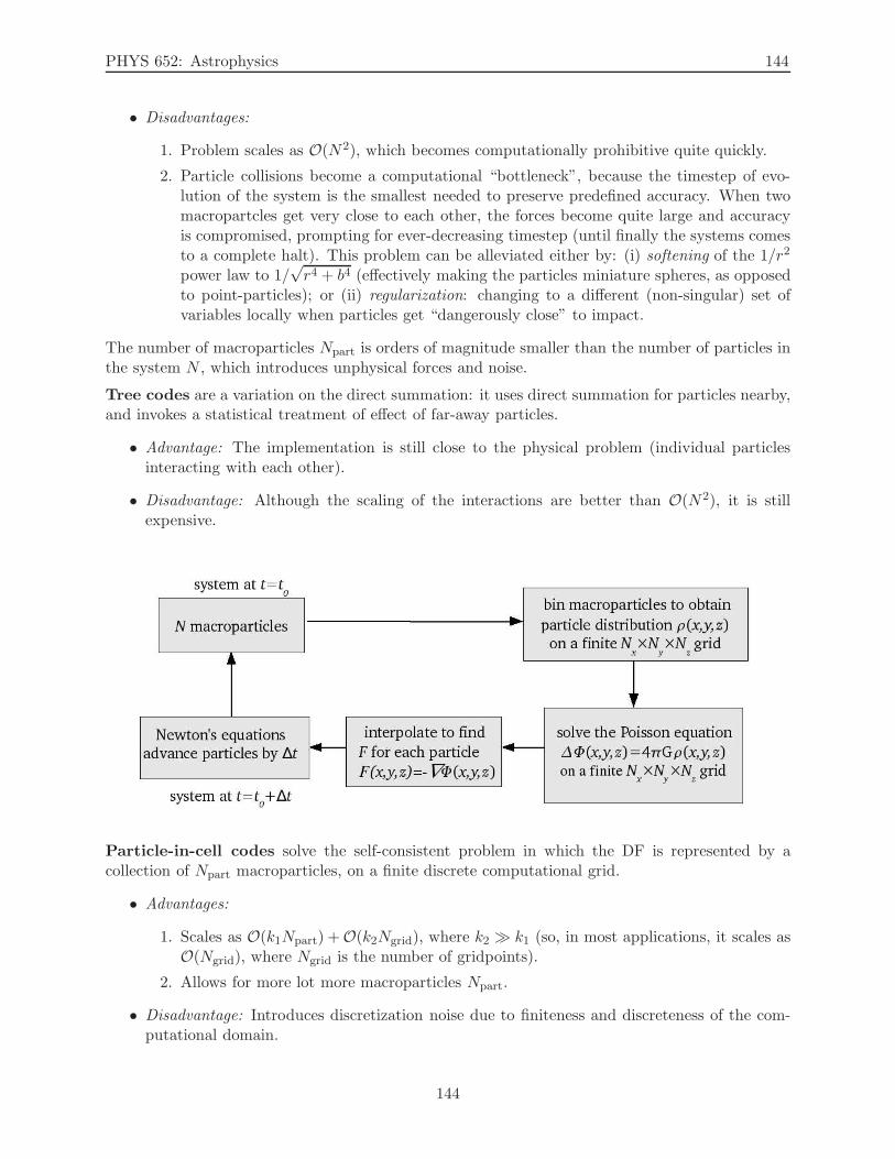
PHYS 652: Astrophysics 144
• Disadvantages:
1. Problem scales as O(N2), which becomes computationally prohibitive quite quickly.
2. Particle collisions become a computational “bottleneck”, because the timestep of evo-lution of the system is the smallest needed to preserve predefined accuracy. When twomacropartcles get very close to each other, the forces become quite large and accuracyis compromised, prompting for ever-decreasing timestep (until finally the systems comesto a complete halt). This problem can be alleviated either by: (i) softening of the 1/r2
power law to 1/√r4 + b4 (effectively making the particles miniature spheres, as opposed
to point-particles); or (ii) regularization: changing to a different (non-singular) set ofvariables locally when particles get “dangerously close” to impact.
The number of macroparticles Npart is orders of magnitude smaller than the number of particles inthe system N , which introduces unphysical forces and noise.
Tree codes are a variation on the direct summation: it uses direct summation for particles nearby,and invokes a statistical treatment of effect of far-away particles.
• Advantage: The implementation is still close to the physical problem (individual particlesinteracting with each other).
• Disadvantage: Although the scaling of the interactions are better than O(N2), it is stillexpensive.
Particle-in-cell codes solve the self-consistent problem in which the DF is represented by acollection of Npart macroparticles, on a finite discrete computational grid.
• Advantages:
1. Scales as O(k1Npart) +O(k2Ngrid), where k2 ≫ k1 (so, in most applications, it scales asO(Ngrid), where Ngrid is the number of gridpoints).
2. Allows for more lot more macroparticles Npart.
• Disadvantage: Introduces discretization noise due to finiteness and discreteness of the com-putational domain.
144
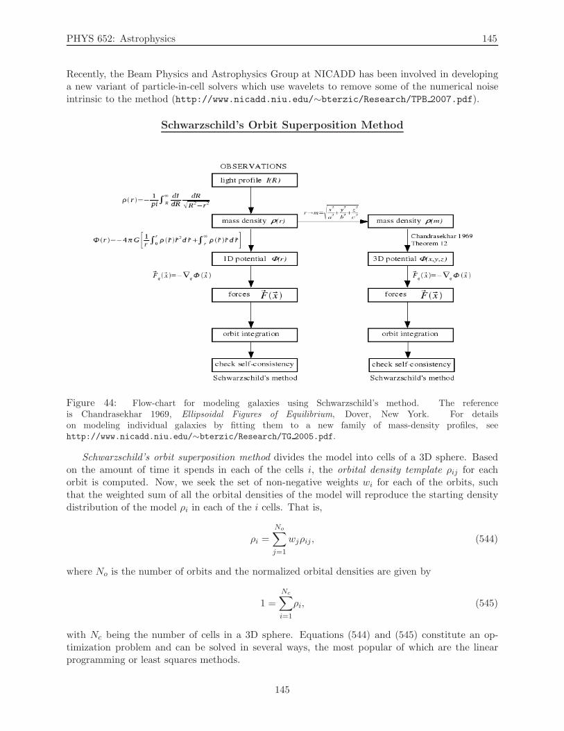
PHYS 652: Astrophysics 145
Recently, the Beam Physics and Astrophysics Group at NICADD has been involved in developinga new variant of particle-in-cell solvers which use wavelets to remove some of the numerical noiseintrinsic to the method (http://www.nicadd.niu.edu/∼bterzic/Research/TPB 2007.pdf).
Schwarzschild’s Orbit Superposition Method
Figure 44: Flow-chart for modeling galaxies using Schwarzschild’s method. The referenceis Chandrasekhar 1969, Ellipsoidal Figures of Equilibrium, Dover, New York. For detailson modeling individual galaxies by fitting them to a new family of mass-density profiles, seehttp://www.nicadd.niu.edu/∼bterzic/Research/TG 2005.pdf.
Schwarzschild’s orbit superposition method divides the model into cells of a 3D sphere. Basedon the amount of time it spends in each of the cells i, the orbital density template ρij for eachorbit is computed. Now, we seek the set of non-negative weights wi for each of the orbits, suchthat the weighted sum of all the orbital densities of the model will reproduce the starting densitydistribution of the model ρi in each of the i cells. That is,
ρi =
No∑
j=1
wjρij, (544)
where No is the number of orbits and the normalized orbital densities are given by
1 =
Nc∑
i=1
ρi, (545)
with Nc being the number of cells in a 3D sphere. Equations (544) and (545) constitute an op-timization problem and can be solved in several ways, the most popular of which are the linearprogramming or least squares methods.
145
PHYS 652: Astrophysics 146
Optimization problem.Schwarzschild’s method is formulated as an optimization problem:
minimize : f (wi),
subject to :No∑
i=1wi ρij = ρj, j = 1, 2, ..., Nc, (546)
wi ≥ 0, i = 1, 2, ..., No ,
where f(wi) is the cost function, ρij is the contribution of the orbital density of the ith template tojth cell, ρj is the model’s density in the jth cell and wi is the orbital weight of the ith orbit. Theproblem above becomes a linear programming problem (LPP) when the cost function is a simple lin-ear function of the weights; for example, to minimize weights of orbits labeled from m to n, the cost
function would simply be f(wi) =n∑
i=mwi. The solutions of the LPP are often quite noisy, with entire
ranges of orbits carrying zero weights. It is often customary to impose additional constraints in or-der to “smoothen” out the solutions, such as minimizing the sum of squares of orbital weights (whichmakes this a quadratic programming problem) or minimizing the least squares. (For an pedagogicaland detailed discourse on the implementation of the Schwarzschild’s method for a special case ofscale-free potentials, see http://www.nicadd.niu.edu/∼bterzic/Research/chapter3.pdf).Chaotic orbits.The orbital density templates ρij are computed so as to represent the time-averaged orbital densityof stars on that orbit, thus making them time-independent building blocks of a time-independentsolution to the self-consistent problem. Chaotic orbits (to be defined later in this lecture) cannothave their individual orbital density templates included into Schwarzschild’s method because theirtime-averaged density would change over time. Instead, chaotic orbits are usually averaged out intoa single chaotic super-orbit orbital template and then included in Schwarzschild method. This isbecause chaotic portion of the phase space in 3 dof (and higher) are interconnected (Arnold’s web),so all chaotic orbits in a given potential can be viewed as parts of one large chaotic super-orbit (i.e.,if integrated long enough — infinitely long — each chaotic orbit will sample all of the availablechaotic phase-space).
Chaos in Galactic Simulations
Decades of numerical simulations have shown that realistic galactic models feature a large num-ber of chaotic orbits. As a case in point, even simple dynamical systems such as the gravitational(restricted) three-body problem features a large portion of chaotic orbits. Another example is anumerical simulation of a 10-body model of a solar system, which found e-folding times for eachof the planets’ orbits in the range of 10 − 50 million years (Laskar 1993, Physica D, 67, 257). Itis then quite reasonable to expect that N-body simulations for which N ≫ 10 will feature chaoticorbits.
In simulations which smooth over particle distribution by invoking a mean-field approximation,such as integration of orbits in a smooth potential, presence of chaos is not nearly as obvious. Thepresence of chaos has only been discovered after the integration of orbits revealed that the numberof integrals of motion was fewer than the number of degrees of freedom (Henon & Heiles 1963,Astronomical Journal, 69, 73).
Definition of chaos: Motion which exhibits sensitive dependence on initial conditions.In other words, nearby orbits will diverge exponentially:
d(t) = d(0)eλt, (547)
146
PHYS 652: Astrophysics 147
where d(0) is the initial separation of nearby orbits, d(t) is the separation of initially nearby orbitsat some later time t, and λ is the Lyapunov exponent.
The Lyapunov exponent is defined as
λ = limt→∞, d(0)→0
1
tln
d(t)
d(0), (548)
and is related to the “e-folding time” τe as τe = 1/λ. The e-folding time denotes a time-scaleafter which one can no longer make quantitative predictions about the system. In other words —loosely speaking — it is the time-scale after which the motion on the same orbit will be completelyuncorrelated.
Here a note of caution is appropriate: the colloquial use of the term “chaotic” has led toa common misconception that chaos implies complete randomness. This is not the case: chaosimplies intrinsic inability to quantify the system beyond the e-folding time.
Regular motion is characterized by vanishing Lyapunov exponents. Orbits are well-defined, havelocalized Fourier spectra, and “appear” regular (”quasi-periodic”). Regular motion in an N -dofsystem is confined by its three integrals of motion to the surface of the N -dimensional torus residingin the 2N -dimensional phase-space.
Chaotic (stochastic, irregular) motion is characterized by non-zero Lyapunov exponents. Or-bits are not well-defined, have “fuzzy” Fourier spectra, and generally “appear” irregular, but notalways: “weakly chaotic” or “sticky” orbits can mimic regular behavior for long periods of time,only to become “wildly chaotic” at later times (short-time Lyapunov exponents can vary drasti-cally). Chaotic motion in an N -dof system is not confined to the surface of the N -dimensionaltorus residing in the 2N -dimensional phase-space, because it does not have N integrals of motion.
Integrable potential have as many integrals of motion as the degrees of freedom. All orbits areregular. Examples of integrable potentials include all spherically symmetric systems (there is nochaos in 1D) and some axisymmetric potentials (2 dof).
Non-integrable potential do not have as many global integrals of motion as the degrees offreedom. However, the presence of local integrals of motion is possible, so there are generally bothchaotic and regular orbits.
Relaxation of Multiparticle Systems
Earlier we computed time needed for the system to reach equilibrium (relaxation time) throughcollisions (close encounters) to be orders of magnitude longer than the Hubble time. This meansthat if close encounters was the only relaxation mechanism at work, we should observe galaxies tobe far from equilibrium. Observations show the contrary: galaxies are to a good approximationrelaxed systems, in (or at least close to) equilibrium. It then became clear that there are othermechanisms at work in driving the system toward equilibrium.
There are several mechanisms believed to be at work in galactic systems, as seen in copiousnumerical studies.
Regular phase mixing (Landau damping) is present in both time-independent and time-dependent systems. It causes ensembles of regular orbits to spread out because of initial spread intheir integrals of motion. If one imagines that nearby orbits reside on slightly different tori, theirconsequent evolution along the surfaces of their respective tori will result in their shear separation(Fig. 46, top panel). The timescale for regular phase mixing depends on: (i) the size of the ensemble
147
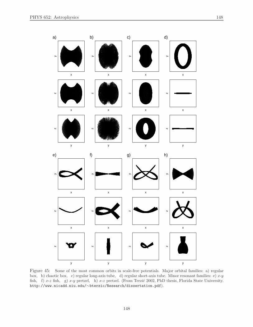
PHYS 652: Astrophysics 148
z
y
z
x
y
x
z
y
z
x
y
x
z
y
z
x
y
x
z
x
y
x
z
y
a) b) c) d)
z
y
z
x
y
x
z
y
z
x
y
x
z
y
z
x
y
x
z
x
y
x
z
y
e) f) g) h)
Figure 45: Some of the most common orbits in scale-free potentials. Major orbital families: a) regularbox, b) chaotic box, c) regular long-axis tube, d) regular short-axis tube. Minor resonant families: e) x-yfish, f) x-z fish, g) x-y pretzel, h) x-z pretzel. (From Terzic 2002, PhD thesis, Florida State University.http://www.nicadd.niu.edu/∼bterzic/Research/dissertation.pdf).
148
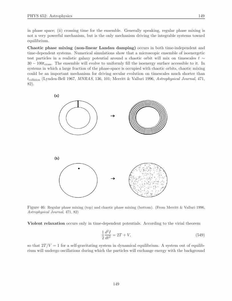
PHYS 652: Astrophysics 149
in phase space; (ii) crossing time for the ensemble. Generally speaking, regular phase mixing isnot a very powerful mechanism, but is the only mechanism driving the integrable systems towardequilibrium.
Chaotic phase mixing (non-linear Landau damping) occurs in both time-independent andtime-dependent systems. Numerical simulations show that a microscopic ensemble of isoenergetictest particles in a realistic galaxy potential around a chaotic orbit will mix on timescales t ∼30 − 100tcross. The ensemble will evolve to uniformly fill the isoenergy surface accessible to it. Insystems in which a large fraction of the phase-space is occupied with chaotic orbits, chaotic mixingcould be an important mechanism for driving secular evolution on timescales much shorter thantcollision (Lynden-Bell 1967, MNRAS, 136, 101; Merritt & Valluri 1996, Astrophysical Journal, 471,82).
Figure 46: Regular phase mixing (top) and chaotic phase mixing (bottom). (From Merritt & Valluri 1996,Astrophysical Journal, 471, 82)
Violent relaxation occurs only in time-dependent potentials. According to the virial theorem
1
2
d2I
dt2= 2T + V, (549)
so that 2T/V = 1 for a self-gravitating system in dynamical equilibrium. A system out of equilib-rium will undergo oscillations during which the particles will exchange energy with the background
149
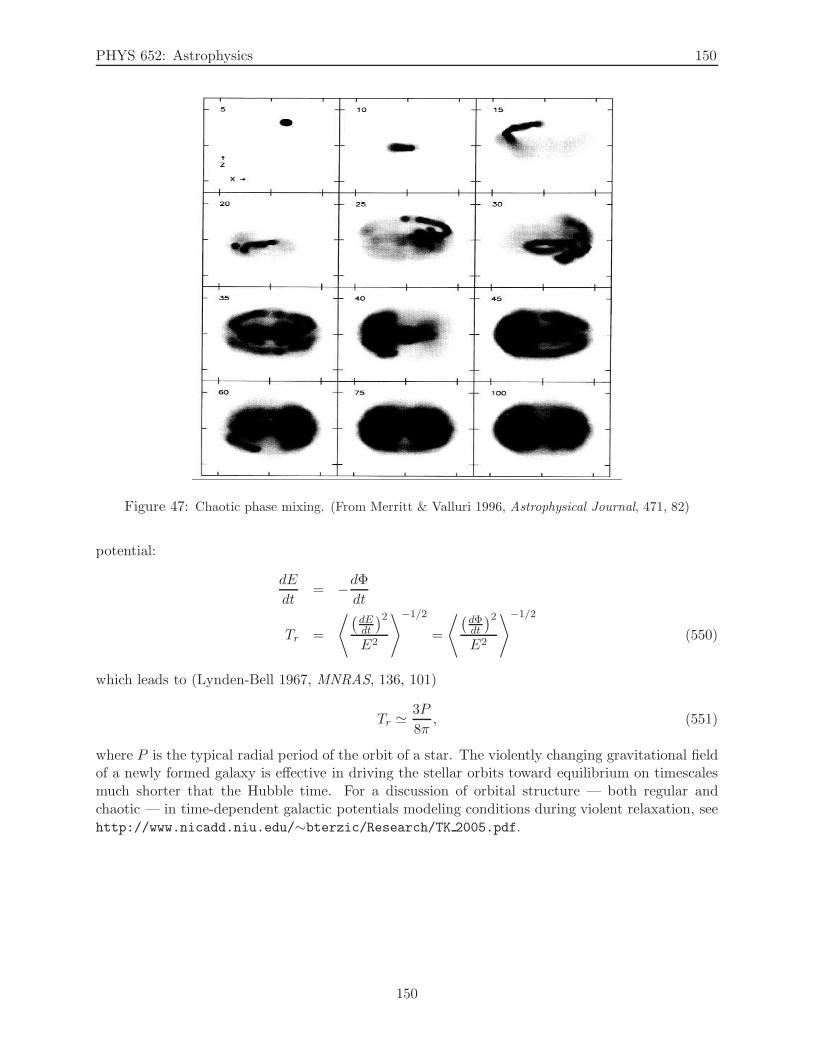
PHYS 652: Astrophysics 150
Figure 47: Chaotic phase mixing. (From Merritt & Valluri 1996, Astrophysical Journal, 471, 82)
potential:
dE
dt= −dΦ
dt
Tr =
⟨
(
dEdt
)2
E2
⟩−1/2
=
⟨
(
dΦdt
)2
E2
⟩−1/2
(550)
which leads to (Lynden-Bell 1967, MNRAS, 136, 101)
Tr ≃3P
8π, (551)
where P is the typical radial period of the orbit of a star. The violently changing gravitational fieldof a newly formed galaxy is effective in driving the stellar orbits toward equilibrium on timescalesmuch shorter that the Hubble time. For a discussion of orbital structure — both regular andchaotic — in time-dependent galactic potentials modeling conditions during violent relaxation, seehttp://www.nicadd.niu.edu/∼bterzic/Research/TK 2005.pdf.
150
PHYS 652: Astrophysics 1
Appendix to Lecture 2
An Alternative Lagrangian
In class we used an alternative Lagrangian
L = gγδxγxδ,
instead of the traditional
L =√
gγδxγxδ.
Here is the justification why either works correctly, i.e., why the expression given in eq. (552) is aLagrangian that generates the geodesic equation.
We prove that by applying the Lagrange’s equations
∂L
∂xα− d
dλ
∂L
∂xα= 0.
to the expression in eq. (552), and recovering the geodesic equation.
∂L
∂xα= gγδ,αx
γxδ,
∂L
∂xα= gαδx
δ + gγαxγ
d
dλ
(
∂L
∂xα
)
= gαδ,γ xδxγ + gαδx
δ + gγα,δxγxδ + gγαx
γ
= (gαδ,γ + gγα,δ) xδxγ + 2gαδx
δ,
because we are at liberty to rename dummy variables (ones which are summed over), and toexchange indices of the metric tensor, since it is symmetric. The Lagrange equation thereforereads:
∂L
∂xα− d
dλ
∂L
∂xα= (gαδ,γ + gγα,δ) x
δxγ + 2gαδxδ − gγδ,αx
γ xδ =
= (gαδ,γ + gγα,δ − gγδ,α) xδxγ + 2gαδx
δ = 0.
Now multiply both sides by 12gνα to isolate the second derivative term:
xν +1
2gνα (gαδ,γ + gγα,δ − gγδ,α) x
δxγ = 0.
But, by definition
Γνβγ =1
2gνα (gαδ,γ + gγα,δ − gγδ,α) ,
so, we finally havexν = −Γνβγx
δxγ ,
which is the geodesic equation we derived in class (eq. (31)). This proves that the Lagrangian ineq. (552) also generates the geodesic equation (the factor of 1/2, or any other positive constant,does not affect the Lagrange’s equations).
Example of Metric Conversion
1
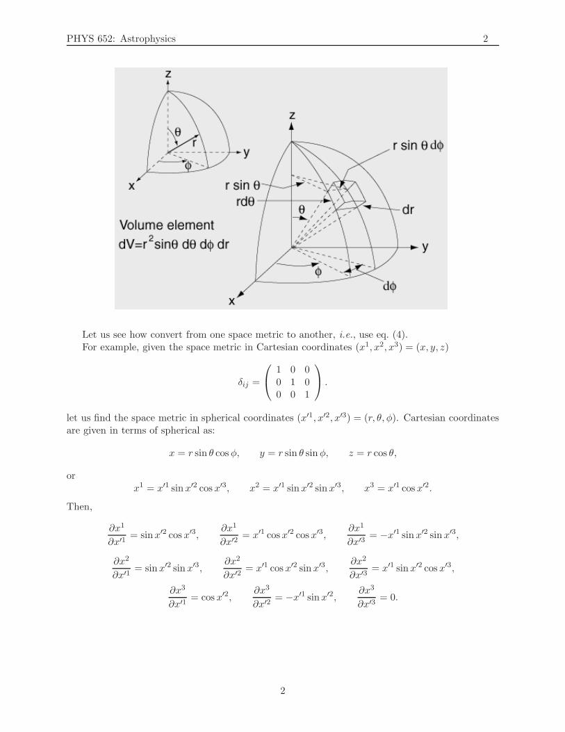
PHYS 652: Astrophysics 2
Let us see how convert from one space metric to another, i.e., use eq. (4).For example, given the space metric in Cartesian coordinates (x1, x2, x3) = (x, y, z)
δij =
1 0 00 1 00 0 1
.
let us find the space metric in spherical coordinates (x′1, x′2, x′3) = (r, θ, φ). Cartesian coordinatesare given in terms of spherical as:
x = r sin θ cosφ, y = r sin θ sinφ, z = r cos θ,
orx1 = x′1 sinx′2 cos x′3, x2 = x′1 sinx′2 sinx′3, x3 = x′1 cos x′2.
Then,
∂x1
∂x′1= sinx′2 cos x′3,
∂x1
∂x′2= x′1 cosx′2 cos x′3,
∂x1
∂x′3= −x′1 sinx′2 sinx′3,
∂x2
∂x′1= sinx′2 sinx′3,
∂x2
∂x′2= x′1 cos x′2 sinx′3,
∂x2
∂x′3= x′1 sinx′2 cos x′3,
∂x3
∂x′1= cos x′2,
∂x3
∂x′2= −x′1 sinx′2,
∂x3
∂x′3= 0.
2
PHYS 652: Astrophysics 3
From eq. (4), we have
ds2 = δijdxidxj
= δij∂xi
∂x′k∂xj
∂x′ldx′kdx′l
= (dx′1)2[
sin2 x′2 cos2 x′3 + sin2 x′2 sin2 x′3 + cos2 x′2]
+ (dx′2)2[
(x′1)2 cos2 x′2 cos2 x′3 + (x′1)2 cos2 x′2 sin2 x′3 + (x′1)2 sinx′3]
+ (dx′3)2[
(x′1)2 sin2 x′2 sin2 x′3 + (x′1)2 sin2 x′2 cos2 x′3]
= (dx′1)2 + (x′1)2(dx′2)2 + (x′1)2 sin2 x′2(dx′3)2
= dr2 + r2dθ2 + r2 sin2 θdφ2
= p11(dr)2 + p22(dθ)
2 + p33(dφ)2
= p11(dx′1)2 + p22(dx
′2)2 + p33(dx′3)2 = pijdx
′idx′j .
Reading off diagonal components of the metric, we have
p11 = 1,
p22 = r2,
p33 = r2 sin2 θ,
so, the space metric for spherical coordinates is
pij =
1 0 00 r2 00 0 r2 sin2 θ
or pij =
1 0 00 1
r20
0 0 1r2 sin2 θ
.
Deriving the geodesic equation in spherical coordinates. Let us now compute the geodesicin 3D flat space, expressed in spherical coordinates. This should be an analog to geodesics in flatspace in Cartesian coordinates:
xα = 0.
This can be done in at least two ways.
Method 1: Brute force – computing Christoffel symbols and substituting them into the geodesicequation. From the eq. (14), Christoffel symbols for the spherical space are given by
Γkij =1
2pkl (pil,j + plj,i − pij,l) .
Since p11 = 1 all of its derivatives vanish. Also, because of symmetry (look at the definition givenin eq. (14) and recall that the metric tensor is symmetric). Therefore, we have
Γk1j = Γkj1 =1
2pkl (p1l,j + plj,1 − p1j,l) =
1
2pklplj,1 =
1
2
(
pk2p2j,1 + pk3p3j,1
)
,
3
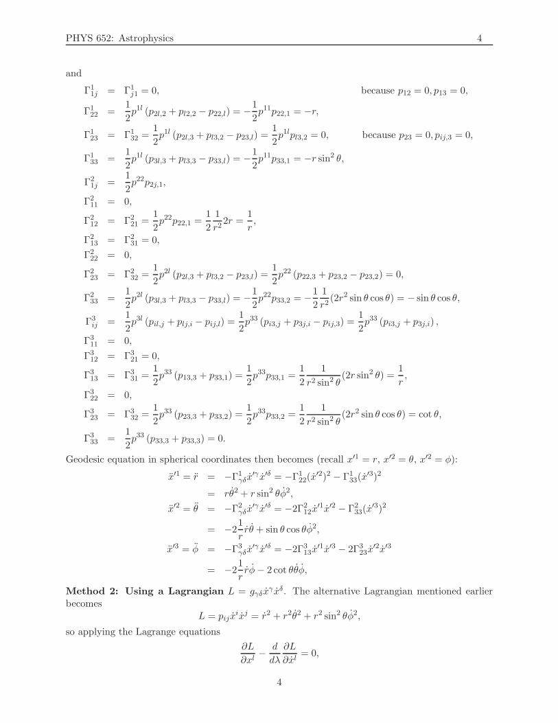
PHYS 652: Astrophysics 4
and
Γ11j = Γ1
j1 = 0, because p12 = 0, p13 = 0,
Γ122 =
1
2p1l (p2l,2 + pl2,2 − p22,l) = −1
2p11p22,1 = −r,
Γ123 = Γ1
32 =1
2p1l (p2l,3 + pl3,2 − p23,l) =
1
2p1lpl3,2 = 0, because p23 = 0, pij,3 = 0,
Γ133 =
1
2p1l (p3l,3 + pl3,3 − p33,l) = −1
2p11p33,1 = −r sin2 θ,
Γ21j =
1
2p22p2j,1,
Γ211 = 0,
Γ212 = Γ2
21 =1
2p22p22,1 =
1
2
1
r22r =
1
r,
Γ213 = Γ2
31 = 0,
Γ222 = 0,
Γ223 = Γ2
32 =1
2p2l (p2l,3 + pl3,2 − p23,l) =
1
2p22 (p22,3 + p23,2 − p23,2) = 0,
Γ233 =
1
2p2l (p3l,3 + pl3,3 − p33,l) = −1
2p22p33,2 = −1
2
1
r2(2r2 sin θ cos θ) = − sin θ cos θ,
Γ3ij =
1
2p3l (pil,j + plj,i − pij,l) =
1
2p33 (pi3,j + p3j,i − pij,3) =
1
2p33 (pi3,j + p3j,i) ,
Γ311 = 0,
Γ312 = Γ3
21 = 0,
Γ313 = Γ3
31 =1
2p33 (p13,3 + p33,1) =
1
2p33p33,1 =
1
2
1
r2 sin2 θ(2r sin2 θ) =
1
r,
Γ322 = 0,
Γ323 = Γ3
32 =1
2p33 (p23,3 + p33,2) =
1
2p33p33,2 =
1
2
1
r2 sin2 θ(2r2 sin θ cos θ) = cot θ,
Γ333 =
1
2p33 (p33,3 + p33,3) = 0.
Geodesic equation in spherical coordinates then becomes (recall x′1 = r, x′2 = θ, x′2 = φ):
x′1 = r = −Γ1γδx
′γ x′δ = −Γ122(x
′2)2 − Γ133(x
′3)2
= rθ2 + r sin2 θφ2,
x′2 = θ = −Γ2γδx
′γ x′δ = −2Γ212x
′1x′2 − Γ233(x
′3)2
= −21
rrθ + sin θ cos θφ2,
x′3 = φ = −Γ3γδx
′γ x′δ = −2Γ313x
′1x′3 − 2Γ323x
′2x′3
= −21
rrφ− 2 cot θθφ,
Method 2: Using a Lagrangian L = gγδxγxδ. The alternative Lagrangian mentioned earlier
becomesL = pijx
ixj = r2 + r2θ2 + r2 sin2 θφ2,
so applying the Lagrange equations
∂L
∂xl− d
dλ
∂L
∂xl= 0,
4
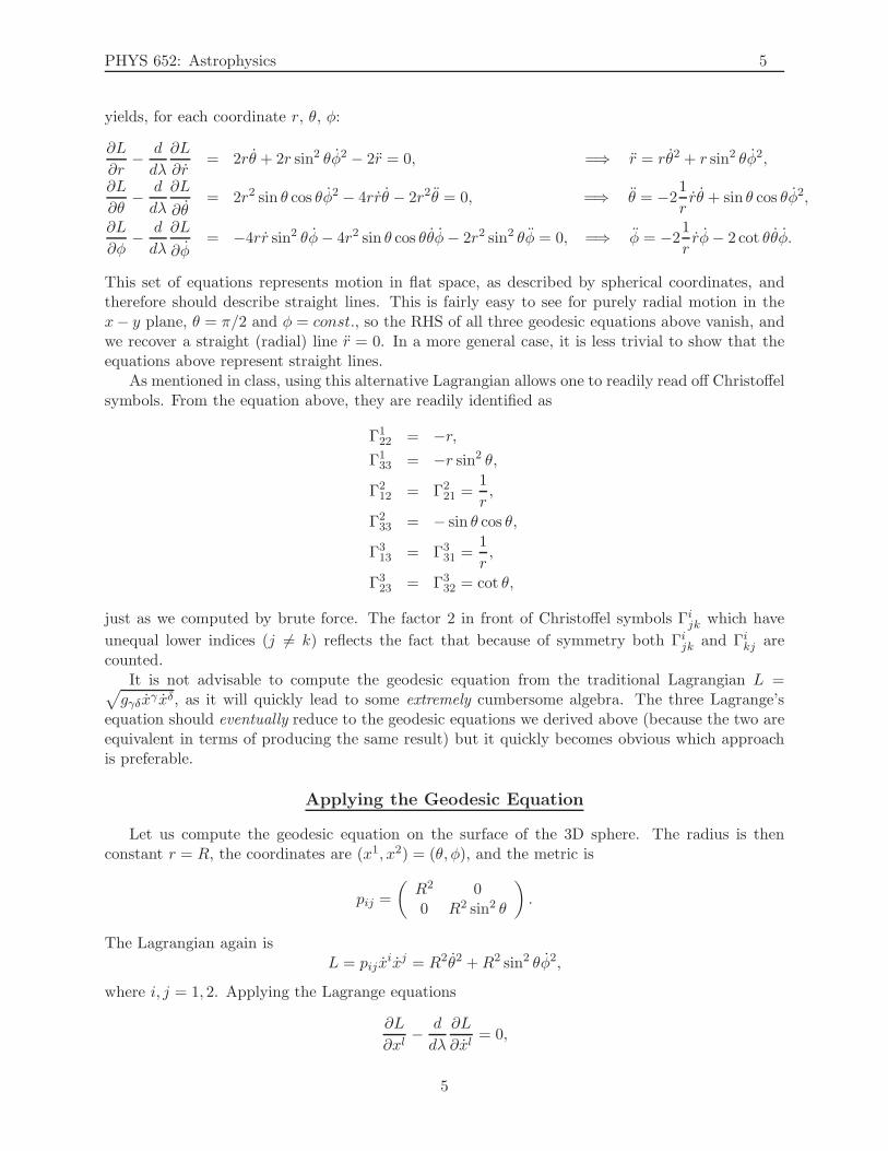
PHYS 652: Astrophysics 5
yields, for each coordinate r, θ, φ:
∂L
∂r− d
dλ
∂L
∂r= 2rθ + 2r sin2 θφ2 − 2r = 0, =⇒ r = rθ2 + r sin2 θφ2,
∂L
∂θ− d
dλ
∂L
∂θ= 2r2 sin θ cos θφ2 − 4rrθ − 2r2θ = 0, =⇒ θ = −2
1
rrθ + sin θ cos θφ2,
∂L
∂φ− d
dλ
∂L
∂φ= −4rr sin2 θφ− 4r2 sin θ cos θθφ− 2r2 sin2 θφ = 0, =⇒ φ = −2
1
rrφ− 2 cot θθφ.
This set of equations represents motion in flat space, as described by spherical coordinates, andtherefore should describe straight lines. This is fairly easy to see for purely radial motion in thex− y plane, θ = π/2 and φ = const., so the RHS of all three geodesic equations above vanish, andwe recover a straight (radial) line r = 0. In a more general case, it is less trivial to show that theequations above represent straight lines.
As mentioned in class, using this alternative Lagrangian allows one to readily read off Christoffelsymbols. From the equation above, they are readily identified as
Γ122 = −r,
Γ133 = −r sin2 θ,
Γ212 = Γ2
21 =1
r,
Γ233 = − sin θ cos θ,
Γ313 = Γ3
31 =1
r,
Γ323 = Γ3
32 = cot θ,
just as we computed by brute force. The factor 2 in front of Christoffel symbols Γijk which have
unequal lower indices (j 6= k) reflects the fact that because of symmetry both Γijk and Γikj arecounted.
It is not advisable to compute the geodesic equation from the traditional Lagrangian L =√
gγδxγ xδ, as it will quickly lead to some extremely cumbersome algebra. The three Lagrange’sequation should eventually reduce to the geodesic equations we derived above (because the two areequivalent in terms of producing the same result) but it quickly becomes obvious which approachis preferable.
Applying the Geodesic Equation
Let us compute the geodesic equation on the surface of the 3D sphere. The radius is thenconstant r = R, the coordinates are (x1, x2) = (θ, φ), and the metric is
pij =
(
R2 00 R2 sin2 θ
)
.
The Lagrangian again isL = pijx
ixj = R2θ2 +R2 sin2 θφ2,
where i, j = 1, 2. Applying the Lagrange equations
∂L
∂xl− d
dλ
∂L
∂xl= 0,
5
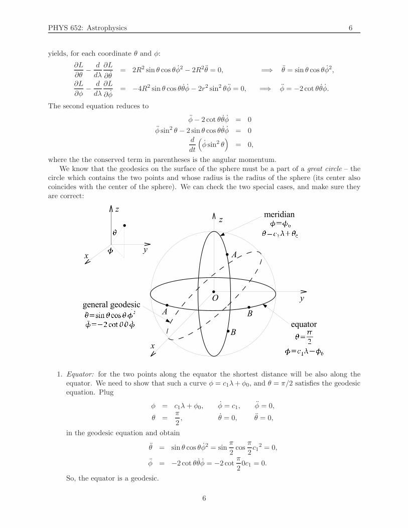
PHYS 652: Astrophysics 6
yields, for each coordinate θ and φ:
∂L
∂θ− d
dλ
∂L
∂θ= 2R2 sin θ cos θφ2 − 2R2θ = 0, =⇒ θ = sin θ cos θφ2,
∂L
∂φ− d
dλ
∂L
∂φ= −4R2 sin θ cos θθφ− 2r2 sin2 θφ = 0, =⇒ φ = −2 cot θθφ.
The second equation reduces to
φ− 2 cot θθφ = 0
φ sin2 θ − 2 sin θ cos θθφ = 0
d
dt
(
φ sin2 θ)
= 0,
where the the conserved term in parentheses is the angular momentum.We know that the geodesics on the surface of the sphere must be a part of a great circle – the
circle which contains the two points and whose radius is the radius of the sphere (its center alsocoincides with the center of the sphere). We can check the two special cases, and make sure theyare correct:
1. Equator: for the two points along the equator the shortest distance will be also along theequator. We need to show that such a curve φ = c1λ+ φ0, and θ = π/2 satisfies the geodesicequation. Plug
φ = c1λ+ φ0, φ = c1, φ = 0,
θ =π
2, θ = 0, θ = 0,
in the geodesic equation and obtain
θ = sin θ cos θφ2 = sinπ
2cos
π
2c1
2 = 0,
φ = −2 cot θθφ = −2 cotπ
20c1 = 0.
So, the equator is a geodesic.
6
PHYS 652: Astrophysics 7
2. Meridian: for the two points along the same meridian (arc of the great circle connecting thetwo poles) the shortest distance should also be along the meridian. We need to show thatsuch a curve φ = φ0, and θ = c2λ+ θ0 satisfies the geodesic equation. Plug
φ = φ0, φ = 0, φ = 0,
θ = c2λ+ θ0, θ = c2, θ = 0,
in the geodesic equation and obtain
θ = sin θ cos θφ2 = sin (c2λ+ θ0) cos (c2λ+ θ0) 02 = 0,
φ = −2 cot θθφ = −2 cot (c2λ+ θ0) c20 = 0.
So, the meridian is a geodesic.
7
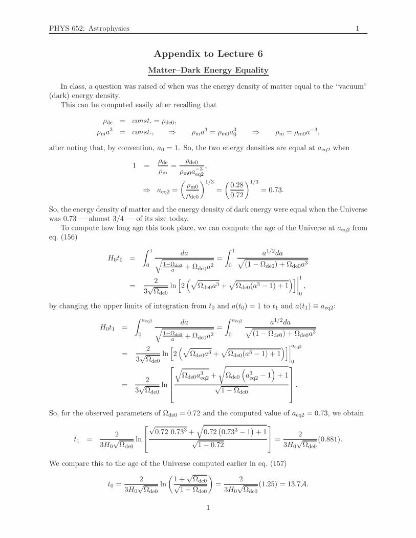
PHYS 652: Astrophysics 1
Appendix to Lecture 6
Matter–Dark Energy Equality
In class, a question was raised of when was the energy density of matter equal to the “vacuum”(dark) energy density.
This can be computed easily after recalling that
ρde = const. = ρde0,
ρma3 = const., ⇒ ρma
3 = ρm0a30 ⇒ ρm = ρm0a
−3,
after noting that, by convention, a0 = 1. So, the two energy densities are equal at aeq2 when
1 =ρdeρm
=ρde0
ρm0a−3eq2
,
⇒ aeq2 =
(
ρm0
ρde0
)1/3
=
(
0.28
0.72
)1/3
= 0.73.
So, the energy density of matter and the energy density of dark energy were equal when the Universewas 0.73 — almost 3/4 — of its size today.
To compute how long ago this took place, we can compute the age of the Universe at aeq2 fromeq. (156)
H0t0 =
∫ 1
0
da√
1−Ωde0a +Ωde0a2
=
∫ 1
0
a1/2da√
(1− Ωde0) + Ωde0a3
=2
3√Ωde0
ln[
2(
√
Ωde0a3 +√
Ωde0(a3 − 1) + 1)]
∣
∣
∣
∣
1
0
,
by changing the upper limits of integration from t0 and a(t0) = 1 to t1 and a(t1) ≡ aeq2:
H0t1 =
∫ aeq2
0
da√
1−Ωde0a +Ωde0a2
=
∫ aeq2
0
a1/2da√
(1− Ωde0) + Ωde0a3
=2
3√Ωde0
ln[
2(
√
Ωde0a3 +√
Ωde0(a3 − 1) + 1)]
∣
∣
∣
∣
aeq2
0
=2
3√Ωde0
ln
√
Ωde0a3eq2 +
√
Ωde0
(
a3eq2 − 1)
+ 1
√1−Ωde0
.
So, for the observed parameters of Ωde0 = 0.72 and the computed value of aeq2 = 0.73, we obtain
t1 =2
3H0√Ωde0
ln
√0.72 0.733 +
√
0.72(
0.733 − 1)
+ 1√1− 0.72
=2
3H0√Ωde0
(0.881).
We compare this to the age of the Universe computed earlier in eq. (157)
t0 =2
3H0√Ωde0
ln
(
1 +√Ωde0√
1− Ωde0
)
=2
3H0√Ωde0
(1.25) = 13.7A.
1
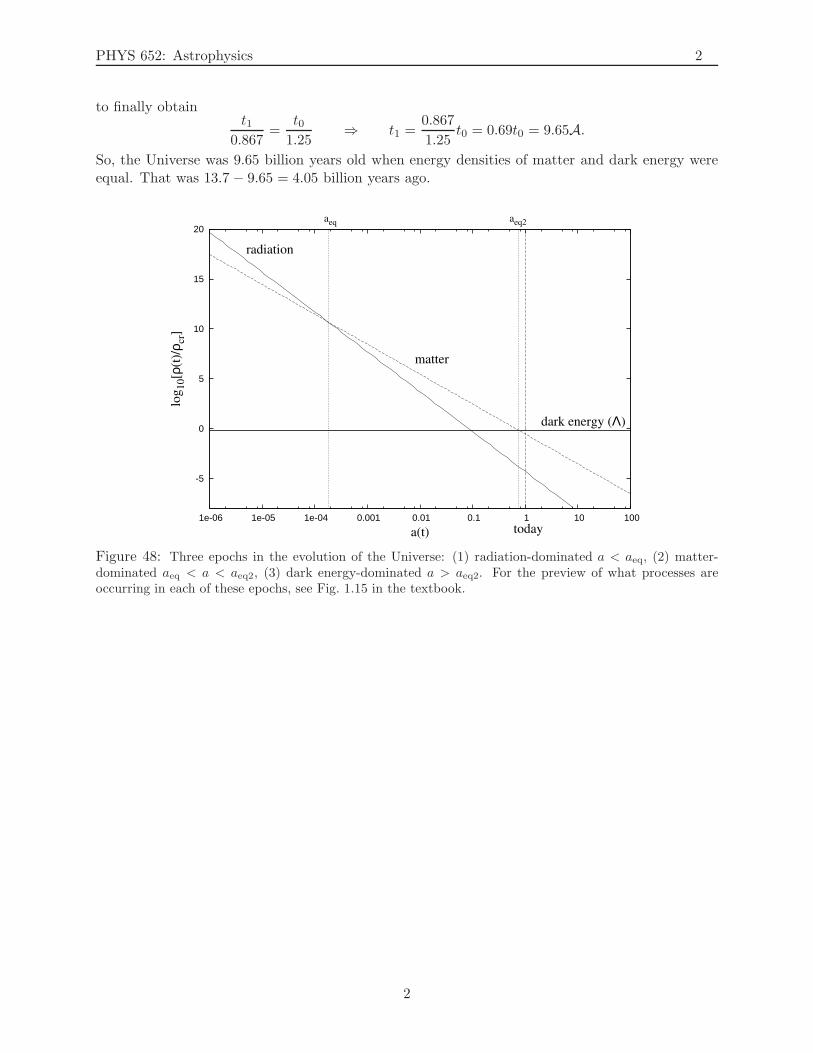
PHYS 652: Astrophysics 2
to finally obtaint1
0.867=
t01.25
⇒ t1 =0.867
1.25t0 = 0.69t0 = 9.65A.
So, the Universe was 9.65 billion years old when energy densities of matter and dark energy wereequal. That was 13.7 − 9.65 = 4.05 billion years ago.
-5
0
5
10
15
20
1e-06 1e-05 1e-04 0.001 0.01 0.1 1 10 100
log
10[ρ
(t)/
ρ cr]
a(t)
matter
radiation
dark energy (Λ)
today
aeq aeq2
Figure 48: Three epochs in the evolution of the Universe: (1) radiation-dominated a < aeq, (2) matter-dominated aeq < a < aeq2, (3) dark energy-dominated a > aeq2. For the preview of what processes areoccurring in each of these epochs, see Fig. 1.15 in the textbook.
2
PHYS 652: Astrophysics 1
Appendix to Lecture 9
Radiation–Dark Energy Equality
In class, a question was raised of when was the energy density of matter equal to the “vacuum”(dark) energy density.
The total energy density of radiation is the sum of the energy density of CMB photons, givenin eq. (209), and the energy density of neutrinos, given in eq. (224), while the energy density ofdark energy is Ωde = Ωde0 = const. We then have:
1 =Ωr
Ωde0=
Ωγ +ΩνΩde0
=2.47×10⁻⁵
h2a4 + 1.65×10⁻⁵
h2a4
Ωde0=
4.12 × 10⁻⁵
Ωde0h2a4
⇒ aeq3 =
(
4.12 × 10⁻⁵
0.72 0.722
)1/4
(≈ 0.1)
⇒ 1 + zeq3 =
(
4.12 × 10⁻⁵
0.72 0.722
)−1/4
(≈ 10) .
where the numbers in parenthesis are given for Ωde0 = 0.72 and h = 0.72.From Friedmann’s first equation:
(
a
a
)2
= H20
[
Ωm0a−3 +Ωr0a
−4 +Ωde0
]
.
Solving for a, this becomes
a = H0
√
Ωm0
a+
Ωr0
a2+Ωde0a2,
and
H0teq3 =
∫ aeq3
0
da√
Ωm0a + Ωr0
a2+Ωde0a2
=
∫ aeq3
0
a da√
Ωm0a+Ωr0 +Ωde0a4
so the age of the Universe for Ωde0 = 0.72, Ωm0 = 0.28, and Ωr0 = 4.12 × 10⁻⁵/h2 = 7.9 × 10⁻⁵ ataeq3 is (after using Maple to perform the calculation):
teq3 ≈ 0.54 A ≈ 5.4× 10⁸ years = 540 million years.
Matter-Radiation Equality
It is beneficial to compute at which point the energy densities of matter and radiation wereequal, because that was the point of transition between these two different regimes. This point iscalled matter-radiation equality. The significance of this transition is that the perturbations in thetwo regimes grow at different rates, as we will see later.
We find the value of the scale factor a(t) = aeq at which the energy densities of matter andradiation were equal by setting their ratio to unity and solving for a.
The total energy density of radiation is the sum of the energy density of CMB photons, givenin eq. (209), and the energy density of neutrinos, given in eq. (224), while the energy density of
1
PHYS 652: Astrophysics 2
baryons is given in eq. (232). We then have:
1 =Ωγ +Ων
Ωm=
2.47×10⁻⁵
h2a4+ 1.65×10⁻⁵
h2a4
Ωm0a−3=
4.12 × 10⁻⁵
Ωm0h2a
⇒ aeq =4.12 × 10⁻⁵
Ωm0h2(
= 2.84 × 10⁻⁴)
⇒ 1 + zeq = 2.43 × 10⁴Ωm0h2(
= 3.52× 10³)
.
where the numbers in parenthesis are given for Ωm0 = 0.28 and h = 0.72. We will see later that thephotons decouple from matter around z ≈ 103, after the matter-radiation equality, which meansthat the decoupling takes place in a matter-dominated Universe.
Let us now estimate how old the Universe was when this happened. From Friedmann’s firstequation:
(
a
a
)2
= H20
[
Ωm0a−3 +Ωr0a
−4 +Ωde0
]
.
Solving for a, this becomes
a = H0
√
Ωm0
a+
Ωr0
a2+Ωde0a2,
and
H0teq =
∫ aeq3
0
da√
Ωm0a + Ωr0
a2+Ωde0a2
=
∫ aeq3
0
a da√
Ωm0a+Ωr0 +Ωde0a4
so the age of the Universe for Ωde0 = 0.72, Ωm0 = 0.28, and Ωr0 = 4.12 × 10⁻⁵/h2 = 7.9 × 10⁻⁵ atat aeq is (after using Maple to perform the calculation):
t0 ≈ 4.8× 10⁻⁵A = 4.8× 10⁴ years ≈ 50000 years.
2
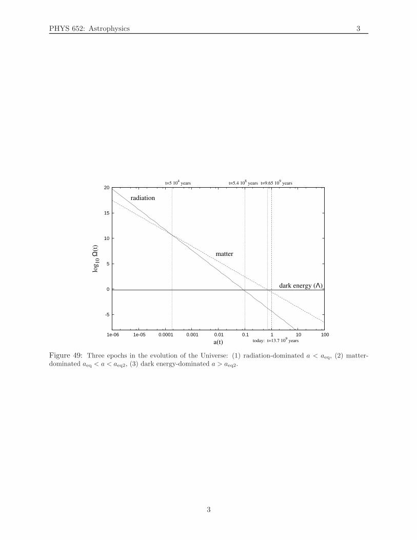
PHYS 652: Astrophysics 3
-5
0
5
10
15
20
1e-06 1e-05 0.0001 0.001 0.01 0.1 1 10 100
log
10 Ω
(t)
a(t)
matter
radiation
dark energy (Λ)
today: t=13.7 109 years
t=5 104 years t=9.65 10
9 yearst=5.4 10
8 years
Figure 49: Three epochs in the evolution of the Universe: (1) radiation-dominated a < aeq, (2) matter-dominated aeq < a < aeq2, (3) dark energy-dominated a > aeq2.
3
PHYS 652: Astrophysics 4
Chemical Potential
The distribution function for species for both fermions and bosons is given by
f =1
e(E−µ)/T ± 1,
(+ for fermions and - for bosons). For a thermal background radiation, the chemical potentialµ is always zero. The reason is the following: µ is defined in the context of the first law ofthermodynamics as the change in energy associated with the change in particle number
dE = TdS − PdV + µdN.
As N adjusts to its equilibrium value, we expect that the system will be stationary with respectto small changes in N . More rigorously, the Helmholtz free energy F = E − TS is minimized(dF/dN = 0) in equilibrium for a system at constant temperature (dT = 0) and volume (dV = 0).Taking the derivative of the Helmholtz energy, we obtain
dF = dE − TdS − SdT,
which, combined with eq. (552), yields
dF = TdS − PdV + µdN − TdS − SdT = −PdV − SdT + µdN
=⇒ dF
dN= −P
dV
dN− S
dT
dN+ µ = µ = 0.
4