16.2 1

16.2 Line Integrals*

x

y

z

Let f (x, y, z) be defined on a region D ∈ R3 containing the smooth

curve C where C is parameterized by

C : r(t) = x(t) i + y(t) j + z(t)k, a ≤ t ≤ b

Recall that C is called a smooth curve of r′ is continuous and r′(t) 6= 0.

* - Some authors also refer to these as “contour integrals”.

16.2 2

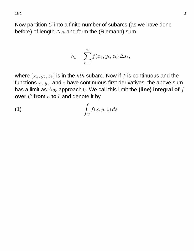
Now partition C into a finite number of subarcs (as we have donebefore) of length ∆sk and form the (Riemann) sum

Sn =n∑

k=1

f (xk, yk, zk)∆sk,

where (xk, yk, zk) is in the kth subarc. Now if f is continuous and thefunctions x, y, and z have continuous first derivatives, the above sumhas a limit as ∆sk approach 0. We call this limit the (line) integral of f

over C from a to b and denote it byˆ

C

f (x, y, z) ds(1)

16.2 3

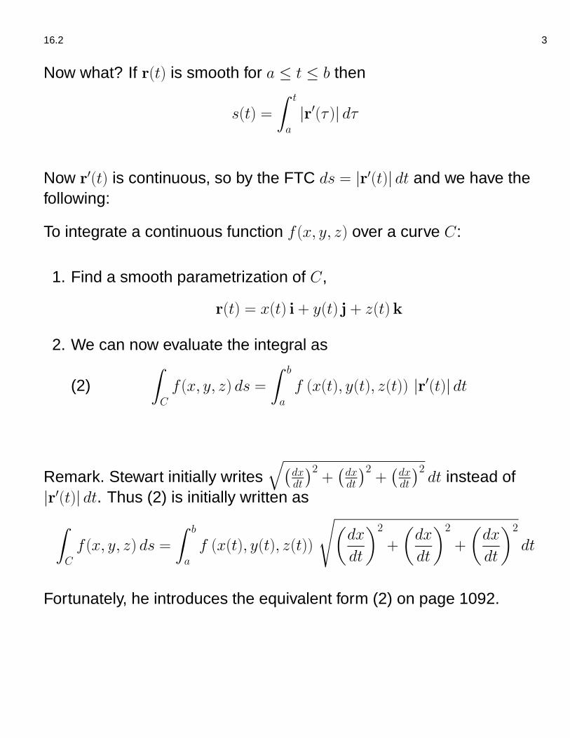
Now what? If r(t) is smooth for a ≤ t ≤ b then

s(t) =

ˆ t

a

|r′(τ )| dτ

Now r′(t) is continuous, so by the FTC ds = |r′(t)| dt and we have thefollowing:

To integrate a continuous function f (x, y, z) over a curve C:

1. Find a smooth parametrization of C,

r(t) = x(t) i + y(t) j + z(t)k

2. We can now evaluate the integral as

(2)ˆ

C

f (x, y, z) ds =

ˆ b

a

f (x(t), y(t), z(t)) |r′(t)| dt

Remark. Stewart initially writes√

(dxdt

)2+(dxdt

)2+(dxdt

)2dt instead of

|r′(t)| dt. Thus (2) is initially written as

ˆ

C

f (x, y, z) ds =

ˆ b

a

f (x(t), y(t), z(t))

√(dx

dt

)2

+

(dx

dt

)2

+

(dx

dt

)2

dt

Fortunately, he introduces the equivalent form (2) on page 1092.

16.2 4

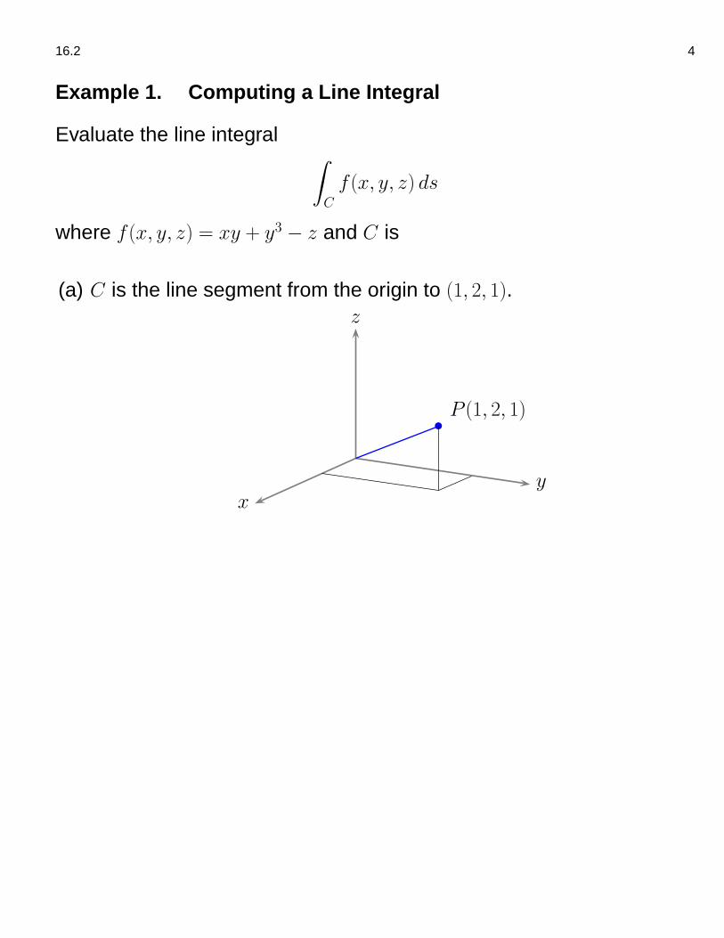
Example 1. Computing a Line Integral

Evaluate the line integralˆ

C

f (x, y, z) ds

where f (x, y, z) = xy + y3 − z and C is

(a) C is the line segment from the origin to (1, 2, 1).

xy

z

bP (1, 2, 1)

16.2 5

Let r(t) = t i + 2t j + tk, 0 ≤ t ≤ 1. Then

f = 2t2 + 8t3 − t

Notice that r(t) is smooth and

|r′(t)| =√

(1)2 + (2)2 + (1)2 =√6

Thusˆ

C

f (x, y, z) ds =√6

ˆ 1

0

(2t2 + 8t3 − t) dt

=√6

(2t3

3+

8t4

4− t2

2

) 1

0

=√6

(13

6

)

16.2 6

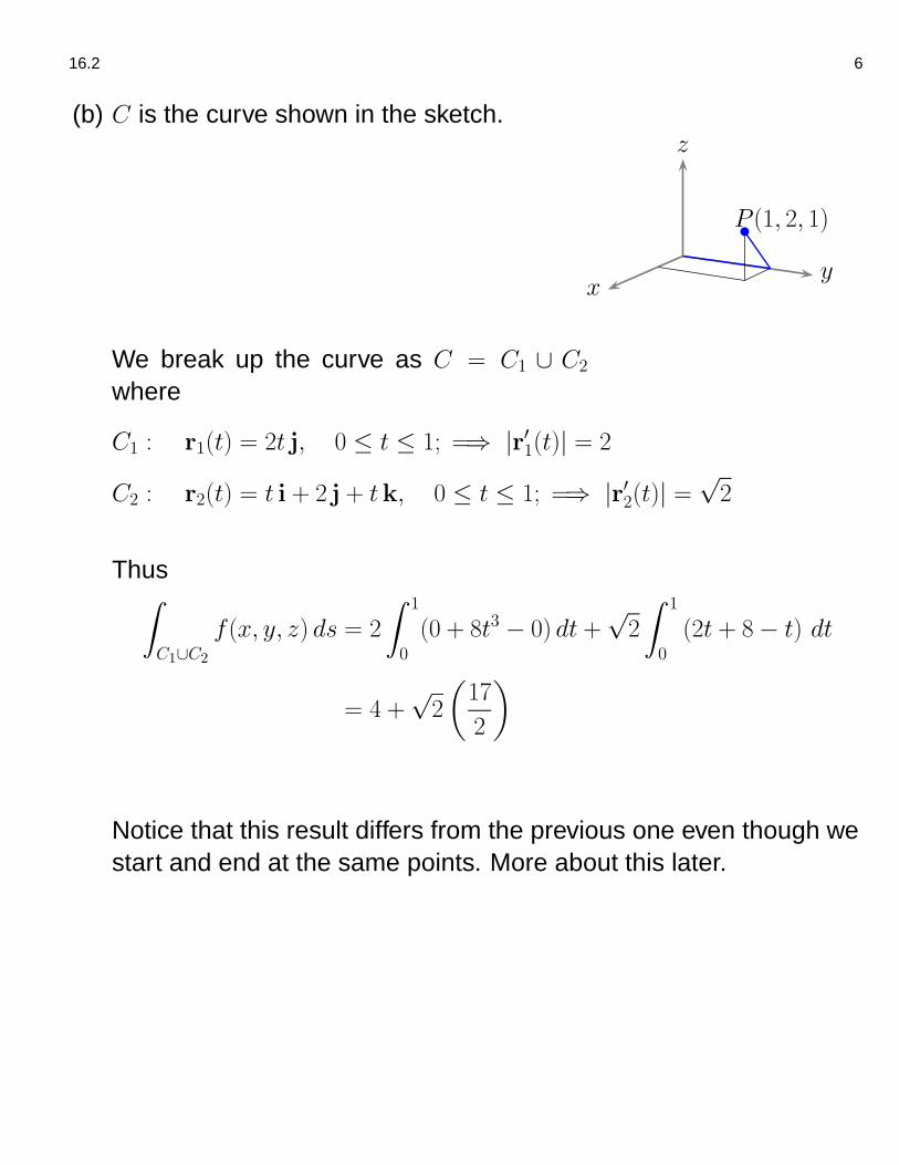
(b) C is the curve shown in the sketch.

xy

z

bP (1, 2, 1)

We break up the curve as C = C1 ∪ C2

where

C1 : r1(t) = 2t j, 0 ≤ t ≤ 1; =⇒ |r′1(t)| = 2

C2 : r2(t) = t i + 2 j + tk, 0 ≤ t ≤ 1; =⇒ |r′2(t)| =√2

Thusˆ

C1∪C2

f (x, y, z) ds = 2

ˆ 1

0

(0 + 8t3 − 0) dt +√2

ˆ 1

0

(2t + 8− t) dt

= 4 +√2

(17

2

)

Notice that this result differs from the previous one even though westart and end at the same points. More about this later.

16.2 7

Work Done by a Force over a Curve

Suppose the vector field

F = M(x, y, z) i + N(x, y, z) j + P (x, y, z)k

represents a force throughout a region in space containing the spacecurve C. Then

Definition. The work done by the force F over the smooth curve C

is given by

(3) W =

ˆ

C

F ·T ds

where T is the unit tangent vector.

Once we choose a (smooth) parameterization, (3) is usually written asˆ

C

F ·T ds =

ˆ t=b

t=a

F ·T ds

where C is parameterized by

r(t) = x(t) i + y(t) j + z(t)k, a ≤ t ≤ b

16.2 8

Remark. Since T = dr/ds we may rewrite (3) asˆ

C

F ·T ds =

ˆ t=b

t=a

F ·T ds

=

ˆ t=b

t=a

F · drds

ds

=

ˆ t=b

t=a

F · dr

where dr = dx i + dy j + dz k.

In fact, we have several different ways to write the work integral:ˆ

C

F ·T ds =

ˆ t=b

t=a

F ·T ds

=

ˆ t=b

t=a

F · dr

=

ˆ b

a

F · drdt

dt

=

ˆ b

a

(

Mdx

dt+N

dy

dt+ P

dz

dt

)

dt

=

ˆ b

a

M dx +N dy + P dz

16.2 9

As we discussed in class, F need not be a force field. See, for example,the notes on flow and flux starting on page 17. We have the following.

Definition. Line Integral of F along C

Let F be a continuous vector field defined on a smooth curve C andsuppose that C is parameterized by a vector function r(t), a ≤ t ≤ b.Then the line integral of F along C is

(4)ˆ

C

F ·T ds =

ˆ b

a

F(r(t)) · r′(t) dt =ˆ t=b

t=a

F · dr

16.2 10

Example 2. Evaluating a Work Integral

Let F = x2 i− y j. Evaluate the integral´

C F ·T ds along the curvex = y2 from (4, 2) to (1, −1).

We try the parametrization (see the next example)

C : r(t) = (2− 3t)2 i + (2− 3t) j, 0 ≤ t ≤ 1

−1 1 2 3

−1

1

2

C

16.2 11

Now

x = (2− 3t)2, dx = −6(2− 3t) dt

y = (2− 3t), dy = −3 dt

Thus

M = x2 = (2− 3t)4

N = −y = −(2− 3t)

and

F · dr = M dx +N dy

= −6(2− 3t)5 dt + 3(2− 3t) dt

so thatˆ

C

F ·T ds =

ˆ 1

0

−6(2− 3t)5 dt +

ˆ 1

0

3(2− 3t) dt

= ...

= −21 + 3/2

16.2 12

Example 3. (Re)Parameterizing a Curve.

How to parameterize the curve y = f (x). Suppose that one wishes toparameterize a given curve from P = (b, f (b)) to Q = (a, f (a)). Onechoice is to set x = s and y = f (s). (Of course, we make the obviousmodifications for the curve x = g(y).) Now

(5) r = s i + f (s) j,

where s lies between a and b. Now if b < a then we are done. On theother hand, if a < b, the parameterization is from Q to P which is notwhat we want.

16.2 13

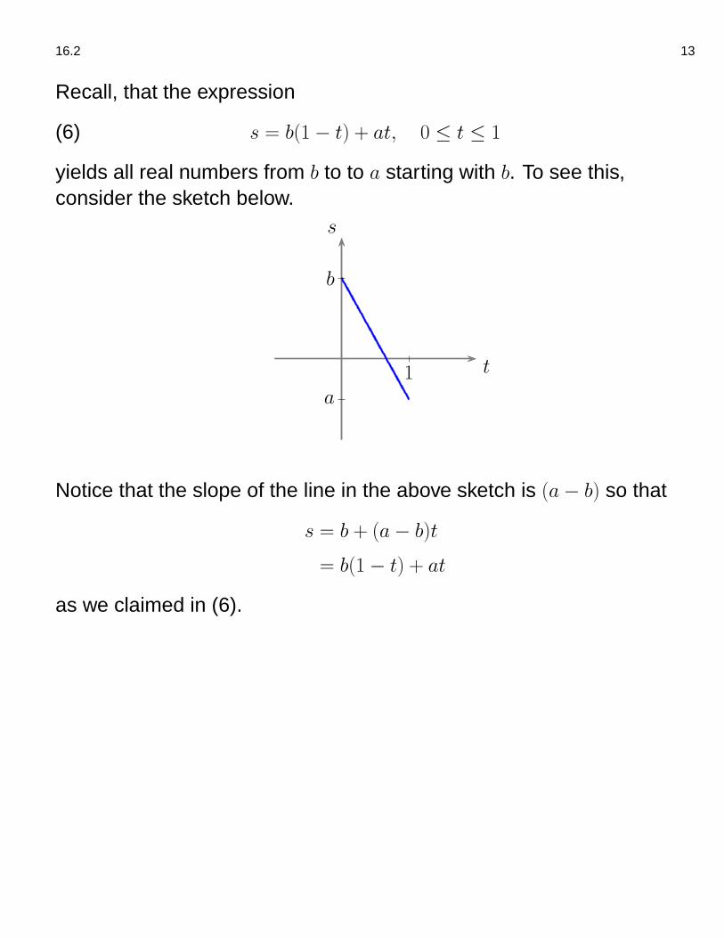
Recall, that the expression

(6) s = b(1− t) + at, 0 ≤ t ≤ 1

yields all real numbers from b to to a starting with b. To see this,consider the sketch below.

1a

b

t

s

Notice that the slope of the line in the above sketch is (a− b) so that

s = b + (a− b)t

= b(1− t) + at

as we claimed in (6).

16.2 14

So let s = b(1− t) + a(t) in (5). It follows that the desiredparameterization is given by

x = b(1− t) + at

y = f (b(1− t) + at), 0 ≤ t ≤ 1

or

(7) r = (b(1− t) + a(t)) i + f (b(1− t) + a(t)) j, 0 ≤ t ≤ 1

As an application, consider the curve x = y2 from the previousexample. In this case the obvious parameterization yields

y = s, x = g(s) = s2, −1 ≤ s ≤ 2

but this traces the curve in the wrong direction. Instead, we apply (7)with

b = 2 and a = −1.

Thus

y = 2(1− t) + (−1)t = 2− 3t

x = (2− 3t)2, 0 ≤ t ≤ 1

as we claimed above.

16.2 15

Example 4. A Calculus II Example

Let a < b. In second semester calculus we saw that the work done by avariable force M(x) directed along the x-axis from x = a to x = b wasgiven by the definite integral

(8) W =

ˆ b

a

M(x) dx

Show that (8) is a special case of (3).

Consider the vector field F(x, y) = M(x) i. Find the work done by theforce F from (a, 0) to (b, 0) along the x-axis.

16.2 16

Notice that we have the parametrization

r(t) = (a(1− t) + bt) i, 0 ≤ t ≤ 1

of the line segment. So r′(t) = (b− a) i and |r′(t)| = b− a. Notice alsothat T = i. It now follows that

W =

ˆ

C

F ·T ds

=

ˆ

C

(M(x) i) · i ds

=

ˆ

C

M(x) ds

=

ˆ 1

0

M(a(1− t) + bt) (b− a) dt︸ ︷︷ ︸

ds

Now let x = a(1− t) + bt. Then dx = (b− a) dt and

W =

ˆ 1

0

M(a(1− t) + bt︸ ︷︷ ︸

x

) (b− a) dt︸ ︷︷ ︸

dx

=

ˆ x(1)

x(0)

M(x) dx

=

ˆ b

a

M(x) dx

as we saw in (8).

16.2 17

Flow Integrals and Circulation

If the vector field

F = M(x, y, z) i + N(x, y, z) j + P (x, y, z)k

represents the velocity field of a fluid flowing through a region in spacethen the integral of F ·T along a smooth curve in the region gives thefluid’s flow along the curve. In that case, we have the following

Definition.

If C is a smooth curve in the domain of a continuous velocity field

F = M(x, y, z) i + N(x, y, z) j + P (x, y, z)k,

then the flow along the curve from t = a to t = b is

(9) Flow =

ˆ

C

F ·T ds

where T is the unit tangent vector. This is called the flow integral . Ifthe curve is a closed loop, the flow is called the circulation around thecurve.

16.2 18

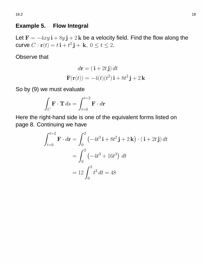
Example 5. Flow Integral

Let F = −4xy i + 8y j + 2k be a velocity field. Find the flow along thecurve C : r(t) = t i + t2 j + k, 0 ≤ t ≤ 2.

Observe that

dr = ( i + 2t j) dt

F(r(t)) = −4(t)(t2) i + 8t2 j + 2k

So by (9) we must evaluateˆ

C

F ·T ds =

ˆ t=2

t=0

F · dr

Here the right-hand side is one of the equivalent forms listed onpage 8. Continuing we have

ˆ t=2

t=0

F · dr =ˆ 2

0

(−4t3 i + 8t2 j + 2k

)· ( i + 2t j) dt

=

ˆ 2

0

(−4t3 + 16t3

)dt

= 12

ˆ 2

0

t3 dt = 48

16.2 19

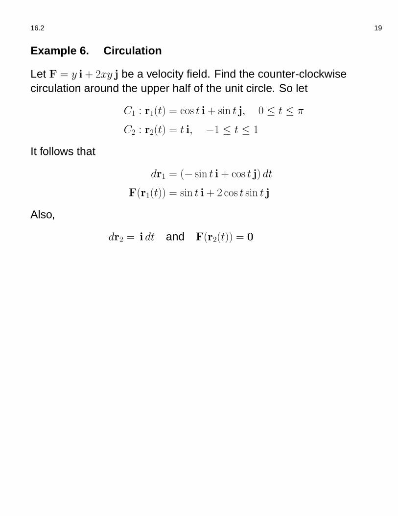
Example 6. Circulation

Let F = y i + 2xy j be a velocity field. Find the counter-clockwisecirculation around the upper half of the unit circle. So let

C1 : r1(t) = cos t i + sin t j, 0 ≤ t ≤ π

C2 : r2(t) = t i, −1 ≤ t ≤ 1

It follows that

dr1 = (− sin t i + cos t j) dt

F(r1(t)) = sin t i + 2 cos t sin t j

Also,

dr2 = i dt and F(r2(t)) = 0

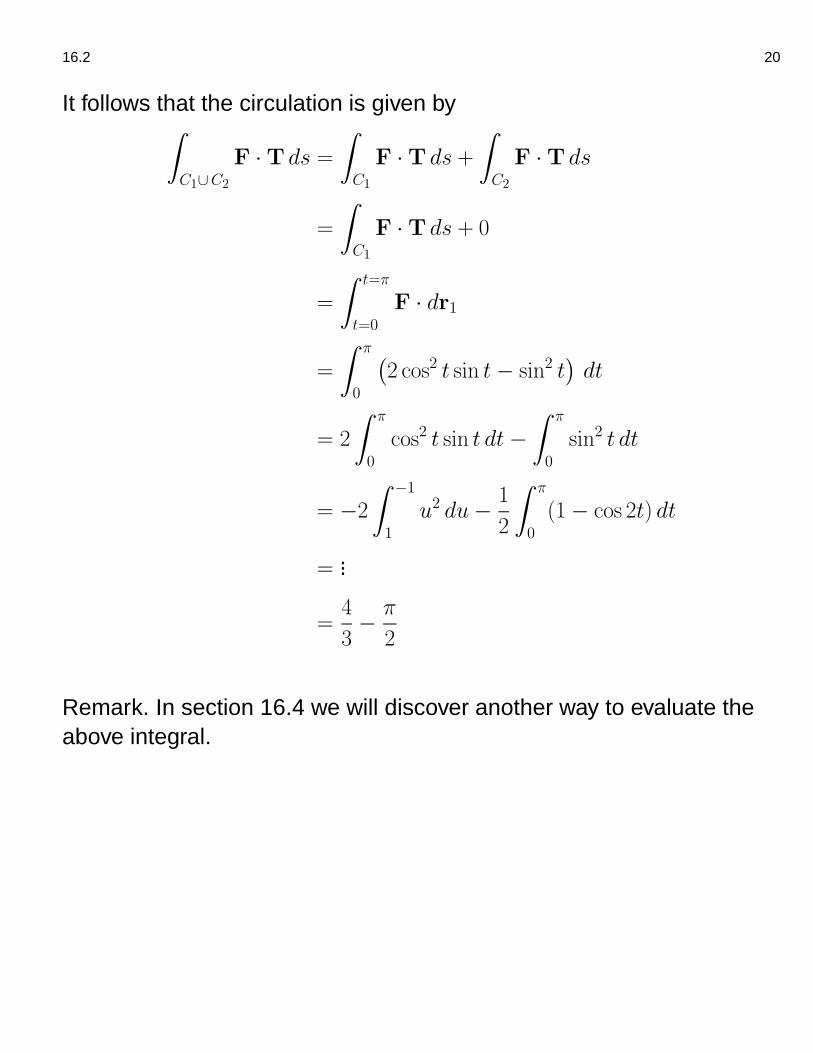
16.2 20

It follows that the circulation is given byˆ

C1∪C2

F ·T ds =

ˆ

C1

F ·T ds +

ˆ

C2

F ·T ds

=

ˆ

C1

F ·T ds + 0

=

ˆ t=π

t=0

F · dr1

=

ˆ π

0

(2 cos2 t sin t− sin2 t

)dt

= 2

ˆ π

0

cos2 t sin t dt−ˆ π

0

sin2 t dt

= −2

ˆ −1

1

u2 du− 1

2

ˆ π

0

(1− cos 2t) dt

= ...

=4

3− π

2

Remark. In section 16.4 we will discover another way to evaluate theabove integral.

16.2 21

Flux Across a Plane Curve

Definition.

If C is a smooth closed curve in the domain of a continuous vectorfield F = M(x, y) i + N(x, y) j in the plane and if n is theoutward-pointing normal vector on C, then the flux of F across C is

Flux =

ˆ

C

F · n ds

Notice that the flux of F across C is the line integral of the scalarcomponent of F in the direction of outward normal.

Now suppose that C is parameterized by

x = x(t), y = y(t), a ≤ t ≤ b

traces the curve in the counterclockwise direction exactly once.

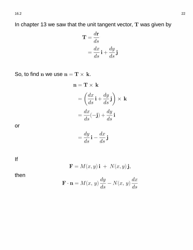
16.2 22

In chapter 13 we saw that the unit tangent vector, T was given by

T =dr

ds

=dx

dsi +

dy

dsj

So, to find n we use n = T× k.

n = T× k

=

(dx

dsi +

dy

dsj

)

× k

=dx

ds(−j) +

dy

dsi

or

=dy

dsi− dx

dsj

IfF = M(x, y) i + N(x, y) j,

then

F · n = M(x, y)dy

ds−N(x, y)

dx

ds

16.2 23

It follows thatˆ

C

F · n ds =

˛

C

(

Mdy

ds−N

dx

ds

)

ds

=

˛

C

M dy −N dx

x

y

z

16.2 24

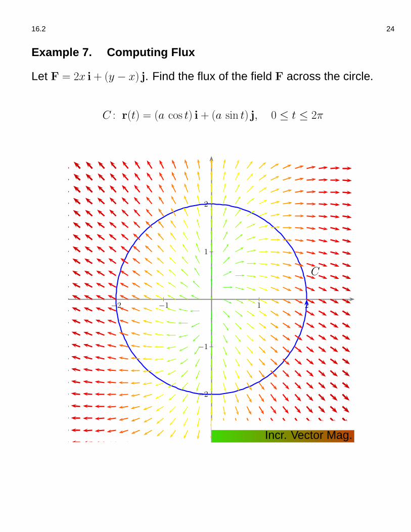
Example 7. Computing Flux

Let F = 2x i + (y − x) j. Find the flux of the field F across the circle.

C : r(t) = (a cos t) i + (a sin t) j, 0 ≤ t ≤ 2π

−2 −1 1 2

−2

−1

1

2

C

Incr. Vector Mag.

16.2 25

x = a cos t, dx = −a sin t dt

y = a sin t, dy = a cos t dt

M = 2x = 2a cos t

N = y − x = a sin t− a cos t

Thusˆ

C

F · n ds =

˛

C

M dy −N dx

=

ˆ 2π

0

2a cos t a cos t dt + (a sin t− a cos t) a sin t dt

= a2ˆ 2π

0

(2 cos2 t + sin2 t− sin t cos t

)dt

= a2ˆ 2π

0

(1 + cos2 t− sin t cos t

)dt

= a2ˆ 2π

0

(

1− sin t cos t +1

2(1 + cos 2t)

)

dt

= a2ˆ 2π

0

(3

2− sin t cos t +

cos 2t

2

)

dt

= a2(3t

2− sin2 t

2+

sin 2t

4

) 2π

0

= 3a2π