1985-02 Spring 1985

SOUTHERN METHODIST UNIVI Optimizing vs. HeuristicMethods for Vehicle Routing

and Scheduling Problems

Christi Hale Sharon Hatcher

LI

OPTIMIZATION VS. HEURISTIC

METHODS FOR VEHICLE

ROUTING AND SCHEDULING PROBLEMS

Christi Hale

Sharon Hatcher

L

.. •... ...

.... .. . •... • •.

•.

DEPARTMENT OF OPERATIONS RESEARCH AND ENGINEERING MANAGEMENT

SCHOOL OF ENGINEERING AND APPLIED SCIENCE

DALLAS, TEXAS 75275

OPTIMIZATION VS. HEURISTIC

METHODS FOR VEHICLE

ROUTING AND SCHEDULING PROBLEMS

Christi Hale

Sharon Hatcher

I

for

OREM 4390, SENIOR DESIGN

May, 1985

ACKNOWLEDGEMENTS

We wish to thank STSC, Inc., of Rockville, Maryland, for their generous support of this project. In particular, we thank Mr. Nanlal Singh for initiating this idea and his encouragement throughout.

DETERMINISTIC VS. HEURISTIC METHODS FOR SOiVING VEHICLE ROUTING AND SCHEDULING PROBLEMS

Distribution costs add about $400 billion each year to the cost of purchased goods in the U.S. alone. The costs associated with operating vehicles and crews for delivery purposes form an important component of total distribution costs. Therefore, even small percentage savings in these expenses could result in substantial total savings over a number of years. And in an increasingly technological society which must take advantage of economies of scale, the relative importance of transportation will continue to grow, and thus routing and scheduling applications will increase in importance.

"Routing and Scheduling" problems refer to the effective management of a fleet of vehicles and associated crews. Private firms that undertake the distribution of their goods to customer locations, and public transportation authorities responsible for providing transportation services to users both rely on routing and scheduling. "Routing problems" give solutions concerning the spatial configuration of vehicle movements, and these problems usually specify a sequence of locations that a vehicle must visit. "Scheduling problems" explicitly consider the times at which various locations are visited. However, in many instances the spatial and temporal characteristics interact and result in "combined routing and scheduling" problems.

An extensive list of applications of routing and scheduling models include mass transit scheduling of vehicles and crews, pick-up and delivery distribution systems, design of dial-a-ride systems, and school-bus routing and scheduling. The area of routing and. scheduling has recently been the focus of intensive research activity. Major advances in this area have been made along both theoretical and applied dimensions.

CLASSIFICATION OF ROUTING AND SCHEDULING PROBLEMS

Basically, the output of all routing and scheduling problems is the same. For each vehicle, a route and a schedule is produced. In general, the route specifies the order that each location will be visited and the schedule designates the times at which the activities at these locations are to be performed.

However, routing and scheduling problems may be classified into one of three major groups: routing, scheduling, or combined

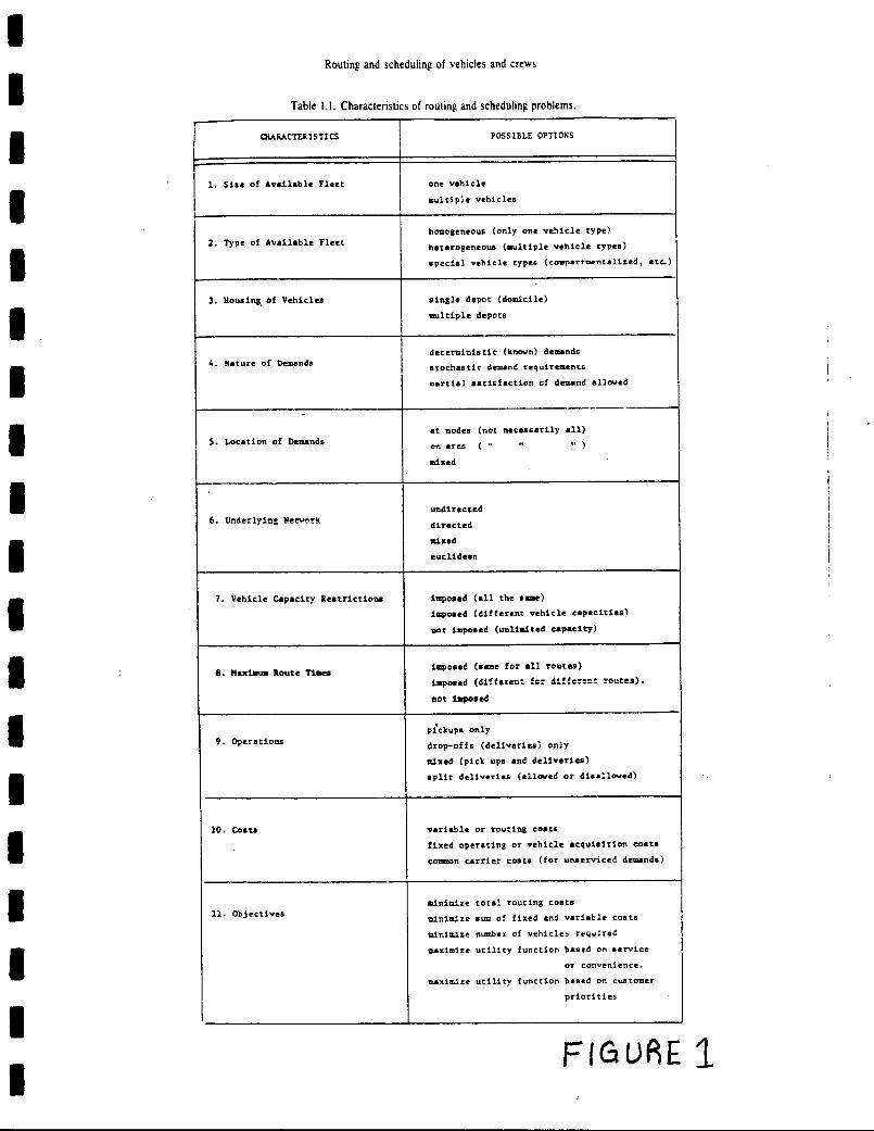
routing and scheduling. Combined routing and scheduling problems may be further subdivided according to a more detailed classification system. Each particular problem is distinguished by characteristics and assumptions that pertain to the given situation. The characteristics, restrictions, and assumptions associated with each problem result in different categories of problems requiring different modeling assumptions. For example, figure 1 (1, P. 73) reveals various combinations of options for eleven characteristics of routing and scheduling problems. Each combination of these various options would result in a problem with unique characteristics.

COMPLEXITY OF ROUTING AND SCHEDULING PROBLEMS

In the formulation and solution of Routing and Scheduling problems, it is important to consider the computational burden associated with various solution techniques. The growth in computation time clearly increases as a function of problem size. In a realistic environment where typical routing and scheduling problems are extremely large, the computation time is prohibitive. Therefore, the applicability of some solution techniques is extremely limited in real-world application.

Since the computational burden in solving these problems grows almost exponentially with problem size, methods of approximation are often resorted to as an alternative to pursuing an optimal solution. The use of heuristics allows for a near-optimal solution. "A heuristic algorithm is a procedure that uses the problem structure in a mathematical (and usually intuitive) way to provide feasible or near-optimal solutions. A heuristic is considered effective if the solutions it provides are consistently close to the optimal solution." (1, P. 76) A powerful heuristic method is defined on the basis of the statistical distribution of answers produced over a range of problems.

EXAMPLES OF HEURISTICS METHODS

A variety of heuristic approaches have found wide use. Here we describe two routing problems and heuristic procedures that have been developed to aid in obtaining near optimal solutions for each type.

2

TRAVELING SALESMAN PROBLEM

cost once.

I

The traveling salesman problem determines the minimal cycle that passes through each node in a network exactly

"Clark and Wright Savings" Method: a heuristic to constuct a tour in a traveling salesman problem. (1) select any node as the central depot (denoted as

(2) compute savings S = C,, , + C Ci for i,j =2,3,..,n.

(3) order the savings from largest to smallest. (4) begin at the top of the savings list and move

downwards, forming larger subtours by linking appropriate nodes i and j. Repeat until a tour is formed.

approach

VEHICLE ROUTING PROBLEM

The vehicle routing problem requires a set of delivery routes from a central depot to various demand centers, each having service requirements, in order to minimize the total distance covered by the entire fleet. The vehicles have specified capacities, and each starts and terminates at the central depot. Two heuristic solution stratgies for vehicle routing problems are the "cluster first-route second" approach, and the "route first-cluster second" approach.

J "Cluster First-Route Second" Approach: groups demand nodes and arcs first and then designs economical routes over each cluster as a second step.

"Route First-Cluster Second" Approach: works in reverse. A large, and usually infeasible

JJ route is constructed which includes all nodes and arcs. Then the large route is partitioned into a number of smaller, feasible routes.

OTHER HEURISTICS (1, p. 99)

MATHEMATICAL PROGRAMMING APPROACHES are based on mathematical programming formulations for the problem.

INTERACTIVE OPTIMIZATION is a general-purpose approach in which a high degree of human interaction is

Ii 3

I I I I

I

incorporated into the problem solving process. The idea is that experienced decision-makers have the capability of setting the revising parameters and injecting subjective assessments based on knowledge and intuition into the optimization model.

THE AVAILABLE TECHNOLOGY TO SOLVE VEHICLE ROUTING AND SCHEDULING PROBLEMS IN COMMERCIAL APPLICATIONS

Until recently, only the larger companies have been able to utilize computer systems in the distribution area. These systems were very effective, but they were expensive to design and maintain. Most of these systems were individually designed and implemented for particular companies, and demanded expensive, on-going, in-house support.

However, with advancing computer technology, smaller, more affordable computers have been designed to meet the needs of smaller companies. Off-the-shelf computer programs currently exist and are less expensive, simpler, and do not demand professional in-house support. These developments have made automated distribution systems feasible for companies of all sizes.

Various software packages designed for the PC help companies solve distribution problems. For example, ROUTEMASTER, offered by Applied Operations Research, Inc., lists for approximately $200. It optimizes the sequence of stops in a single truck route, minimizing time or mileage, and cost. However, ROUTEMASTER is not as intelligent as some other packages, and it ignores several important variables. A more complex package is TRUCKSTOPS offered by MicroAnalytics for a little over $900. Although TRUCKSTOPS is more expensive, it is also much more intelligent. This package designs a route for each truck and sequences the stops on that route to minimize the total route cost in terms of mileage, time, and overtime.

TRUCKS, offered by STSC, is perhaps one of the most complex and intelligent of the software packages available for solving routing and scheduling problems. This remarkable package is used by companies such as Frito-Lay, Safeway, and Martin-Brower, which services McDonald's. TRUCKS sells for approximately $175,000. The package is heuristics-based, but it takes into consideration almost any constraining condition imaginable. The system parameters that have a significant influence on the routing

4

operation of the package are listed and described below. (2, pp. 631-641) These parameters are divided into three groups according to the level of importance in the routing operation. Type A constraints are the most fundamental to model, Type B constraints are somewhat difficult to model and moderate in importance, and Type c constraints are the most luxurious and the most difficult to model. And some constraints range from Type A to Type c depending on the complexities involved.

TYPE A CONSTRAINTS

MAXIMUM ROUTE ON-DUTY-TIME This constraint limits the number of hours a driver may be

on duty. On-duty time is the sum of all load and unload times, (pre-trip and post-trip), all driver wait times, and total route drive time. In our model we limit each driving team's on-duty time to a 48-hour maximum.

MAXIMUM ROUTE DISTANCE This constraint limits the total distance of any single

route. In our model we put a different limit on each route. We limit route A to 500 miles, route B to 600 miles, and route C

to 450 miles.

SERVICE TIME AT EACH LOCATION This constraint limits the service time at each stop along a

route, and is based on some base unload rate multiplied by the quantity unloaded. Our model assumes the base unload rate is six minutes/pallet, which converts to 0.10 hour/pallet. Multiply the unload rate by the quantity unloaded to obtain the service time at each location.

PRE-TRIP TIME This time is actually considered part of a route. It is the

time at the beginning of a route that accounts for administrative overhead, equipment inspections, etc. Our model assumes pre-trip time to be 30 minutes.

POST-TRIP TIME This time is also considered part of a route. It is the

time at the end of a route allocated for a driver to end a route. Our model assumes post-trip time is 15 minutes.

LENGTH OF ROUTING CYCLE This constraint limits the length of time within which all

vehicles used in the routing cycle must be dispatched and returned. Our model assumes the maximum length of the routing cycle to be five days.

5

III

MAXIMUM STOPS PER ROUTE This constraint sets a maximum number of stops allowed for each route. The constraint is used to control the maximum size of any route generated. The domicile stop at each end of the route is included in the number of stops in a route. Our model sets a maximum of three stops per route.

MAXIMUM ORDERS PER ROUTE This constraint sets a maximum number of orders allowed for

a single route. Our model assumes that an order equals a stop. Therefore, there is a maximum of three stops per route also.

LOCATION WINDOWS These constraints limit the times that a particular location e an order. This window applies to all orders is open to receiv

picked up or delivered at a particular location. For example, location X is open to receive orders only from 6 a.m. t.o 8 a.m.

every day.

ASSIGNED DOMICILE A specific domicile (or central depot) can be assigned to certain distribution areas. This forces these distribution areas to be serviced by vehicles originating only from the

designated domicile. Our model assumes that one domicile

(Dallas) services six customers.

TYPE B CONSTRAINTS

CAPACITY VS. TRAILER TYPE Our model assumes one unit of measure for the loads

(pallets) as oosed to multiple units of measure (weight,

volume, pallets)pp

. Our model assumes that we have multiple nt capacity. The capacity of

trailer types each with a differe vehicle A is 30 palettes, vehicle B is 40 palettes, and vehicle C

is 25 palettes.

MAXIMUM CAPACITY PERCENTAGE or MAXIMUM TRAILER LOAD This constraint limits the capacity on each vehicle during a

route. The capacity of the vehicle type is considered when determining the total load on a trailer as stops are added to the route. We assume that all three vehicles are only loaded to 90 percent capacity. Therefore the maximum load on vehicle A is 27 palettes, on vehicle B it is 36 palettes, and on vehicle C it is

22 palettes.

MAXIMUM SHIFT TIME This constraint limits the maximum number of on-duty hours

6

(including pre-trip time, post-trip time, load and unload times, and driver wait times) a driver may have before a lay-over is required. This constraint applies only to domicile locations and restricts shift times for routes run from that domicile.

MAXIMUM DRIVE TIME This constraint limits the maximum number of driving hours

only before a lay-over is required. This constraint also applies only to domicile locations and restricts drive times for routes run from that domicile.

MAXIMUM WAIT TIME AT A STOP This constraint limits the amount of time a vehicle may wait

at a location before the time windows are open. Wait time provides some flexibility, especially when time windows tend to be very tight. Our model assumes that maximum wait time at a stop must not exceed four hours.

MAXIMUM TOTAL WAIT TIME IN A ROUTE This constraint limits the total sum of all wait times for

all stops in a route.

MAXIMUM ROUTES AVAILABLE This constraint limits the maximum number of routes that may

be dispatched in a given time period.

ORDER WINDOWS This constraint specifies the earliest and latest pick-up

and delivery dates and times allowed for each order. Order windows are used to further restrict the handling of an order because they restrict the time a particular order is handled at a location.

TYPE C CONSTRAINTS

ORDER WANDER LIMIT The order wander measures for each step the ratio between a

particular route distance and a direct line distance from the route origin. A low ratio acts as a limit on the amount of "wandering" the Router can do to fit new routes into the schedule.

ROUTE WANDER LIMIT The route wander measures for each stop the ratio between

the total route distance developed so far and the minimum route distance to service the orders. The ratio helps keep a route from crossing over itself and increasing mileage.

7

MINIMUM DISTANCE FOR SMOTR/TEAM ROUTES This constraint limits the total route distance before a route will be considered no longer a "local" route, but a single-man-over-the-road (SMOTR) route or a team route.

SINGLE-TO-TEAM CUTOVER TIME The cutover time constrains the maximum allowable length of a route run by a single driver, ignoring the length of a shift. Once a route is no longer considered "local" and has been assigned as a SMOTR, if the single-to-team cutover time limit is exceeded, the route is considered for assignment to a team.

SINGLE-TO-TEAM CUTOVER DISTANCE cutover time limit or the If either the single-to-team

single-to-team cutover distance limit is exceeded, the SMOTR will

become a team.

ADDITIONAL CAPACITY PERCENTAGE This parameter measures how much more capacity a trailer can have during a route if it is not already empty. it permits control over the amount of cargo shifting necessary during a route with mixed pick-up and deliveries.

MINIMUM REDISPATCII TIME

t

This constraint sets the time to be allowed unscheduled between successive dispatches of the same vehicle and driver. This constraint does not include the time at the domicile.

I BASE COST MARGIN The base cost for an order is calculated for each available

I

domicile based on that domicile's stated equipment cost per mile

and the distance necessar y to service the order. Any domicile

whose base cost falls outside this limit will not be considered as a domicile for this order. This margin allows the router to

Iomicile to service

choose a suitable dvice a set of orders in a

multiple domicile situation. This constraint would pply to ld not

our model since we assume a single assigned domicile.

1 ROUTING CYCLE OVERLAP Routing cycle overlap allows a route to be dispatched in one cycle and return in the next cycle as long as the total route length plus any redispatch time requirement does not exceed the

length of one full cycle.

This constraint sets a minimum on the amount of lay-over II

MINIMUM LAYOVER

time of routes originating at the corresponding domicile

location.

II8

21

MAXIMUM LAYOVER This constraint sets a maximum on the above.

TIME ZONES This parameter takes into account the fact that routes may

cross into different time zones. This constraint would not apply to our model since we are routing only through the Texas, Louisiaflna, Arkansas, Oklahoma areas.

PRODUCT CLASS VS. TRAILER TYPE The product class of an order must be compatible with the

classes of other orders on the same trailer. This constraint would not apply to our model since we assume only a single product class, OR1.

ORDER FREQUENCY AND MINIMUM SPACING Order frequency is the number of times the order is to be

serviced in a single routing cycle, and the spacing is the minimum time to be allotted between deliveries. This creates multiple duplicate orders of the same kind.

RANGES OF CONSTRAINT TYPES

Some of the Type A constraints may range to Type B and Type C constraints with added complexities.

LOCATION WINDOWS A Type A constraint on location windows assumes that there

is one window open to receive an order at the same time each day. However, a Type B constraint would occur with multiple windows open any day, and a Type C constraint would occur with multiple windows open only on specific days.

CAPACITY VS. TRAILER TYPE Our constraint is a Type B. We assume one unit of measure

(pallets, and multiple trailer types. A simpler Type A constraint would assume one unit of measure and one trailer type, while a more complex Type C constraint would assume multiple units of measure and multiple trailer types.

DOMICILE Our model assumes the Type A constraint that we have a

single domicile. However, a more complex Type B or C constraint could assume multiple domicile locations.

SERVICE TIME AT EACH LOCATION Our model's Type B constraint assumes the service time is

determined by the set unload rate multiplied by the quantity unloaded. A simpler Type A constraint would assume a base unload time not related to the quantity unloaded. A more complex Type C constraint would assume various unload rates for various product classes at various delivery locations.

OBJECTIVE FUNCTION Our model assumes a Type A objective function that we

minimize cost (with cost in terms of miles). More complex

objective functions would result if we minimized more than one

variable type. For example, we could minimize cost or miles,

hours, and number of vehicles required, all in the same objective

function.

OUR MIXED INTEGER PROGRAMMING MODEL

Our simplified model of a routing and scheduling problem is based on a distribution network with one central depot which distributes goods to a large region. The input data is a set of orders from six customers during one business week. (See figure 2) The distribution center has three trucks available to make deliveries, each with a different capacity and route-mileage limit.

In the model, we formulated first what we believed to be the most fundamental constraints, such as the miximum distance each truck can travel, and "subtouring" constraints to insure that the trucks return home to the central depot. With that accomplished, we sought to add constraints which would be valuable in making our model simulate a real-world situation. Our choice was limited by the fact that we were programming in LINDO, which processes a maximum of 400 constraints. The most dificult but necessary constraint of those we chose was the arrival-time constraint, which forces delivery to occur within a time interval specified by the customer. This feature alone represents over 200 constraints in the mixed integer program; over half of the total number of constraints.

An example of a feature we did not include because of the complexity it would add to the model is a maximum-number-orders for trucks' routes. We assume in our model that one stop is equivalent to one order, but in a real-world situation, one stop may have multiple orders. Another example is having both location windows and delivery windows; our model is limited to one set of windows.

10

The variables, constants, and assumptions of the model are

as follows:

VARIABLES

0-1 integer variable representing an arc from node (customer) i to node j for truck v. For seven nodes (one depot and six customers) and three trucks, there are 126 's.

AiArrival time at node j; Aj represents arrival time at the previous node i.

wJ Wait time at node j for truck v.

U, Uj Variables associated with nodes i and j, employed in the subtouting—elimination constraints.

CONSTRAINT PARAMETERS

n = 7 : Number of nodes.

V = 3 : Number of vehicles (trucks) available.

Ci,. Capacity of truck V in pallets. C, = 30, C = 40, C3 = 25

P = 90 : Percent loading capacity of each truck, effectively making C, = 27, C 2 = 36, C3 = 22.

= Demand (quantity ordered) at node i in pallets. q, =0 qg=6 q2 =12 q= 16 q3 =18 q7=6 q 4 18

d ij = Distance from node i to node j in miles.

D = Maximum route distance for truck v. = 500, D 2. = 600, D3 = 450

T = 48 : Maximum route—time allowed in hours.

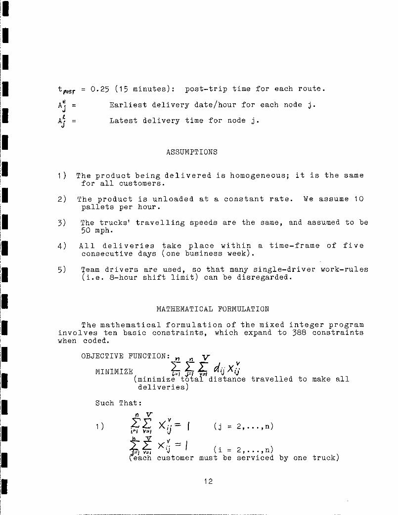
t E = 0.5 (30 minutes): pre—trip time for each route.

I I

= 0.25 (15 minutes): post-trip time for each route.

A = Earliest delivery date/hour for each node j.

I Aj = Latest delivery time for node j.

ASSUMPTIONS

1) The product being delivered is homogeneous; it is the same for all customers.

2) The product is unloaded at a constant rate. We assume 10

pallets per hour.

3) The trucks' travelling speeds are the same, and assumed to be 50 mph.

4) All deliveries take place within a time-frame of five consecutive days (one business week).

5) Team drivers are used, so that many single-driver work-rules (i.e. 8-hour shift limit) can be disregarded.

MATHEMATICAL FORMULATION

The mathematical formulation of the mixed integer program involves ten basic constraints, which expand to 388 constraints when coded.

OBJECTIVE FUNCTION: v

i. MINIMIZE 1 &.ZZ dJXI :I j -:1 vs

(minimize total distance travelled to make all deliveries)

Such That:

1) f (j = 2, ... ,n)

Af >< (1 = 2, ... ,n) (each customer must be serviced by one truck)

12

VIri

VV

X (v 2) -° P FJ =

p = 1,...,fl

(route continuity must be preserve d i.e. if

a truck visits customer i, it must leave

customer i)

x) (v = i,...,V)

(the trucks' capacities cannot be exceeded for deliveries on an assigned route)

ZZ j ^ v (v =

VI J-' (maximum route distance for each truck cannot

be exceeded)

VI

5) A 11 VI

^ T- tEPO+(v =

J-I Assuming unload rate = 6 mm/pallet,

driving speed = 50 mph. (total route—time must not exceed maximum T)

(arrival time must fall within window specified by customer)

V1 M

)( I 3 (v = i,...,v)

t= I ( (maximum number of stops per route is 3)

8)( + 0. 10 ôozd i + y) - (i- x.)T

A (Af oia O.O2d1 J) Y)T

for all i, j, v (arrival time formulation)

13

( j = 2,... ,n = 9)

(maximum wait—time at a customer stop is 4 hours)

10)

( i =2,... 1 n; j = 2,...,n; V =

(subtours are not truck must return route completion)

allowed; truck must to central depot for

PROBLEM SOLUTION---MIP

When we attempted to run our program on LINDO, we found that although we had stayed within the limits for the total number of constraints and variables, it could not solve the problem. The obstacle was our 126 integer variables. Although LINDO has a capacity of 599 variables, it cannot handle nearly as many integer variables.

Our alternative was to solve the problem on the MPSX (Mathematical Programming System) package on the IBM computer.

LINDO has a feature to convert a mixed integer problem to the MPS input format required. After converting our problem, MPS was able to solve it successfully.

RESULT SUMMARY

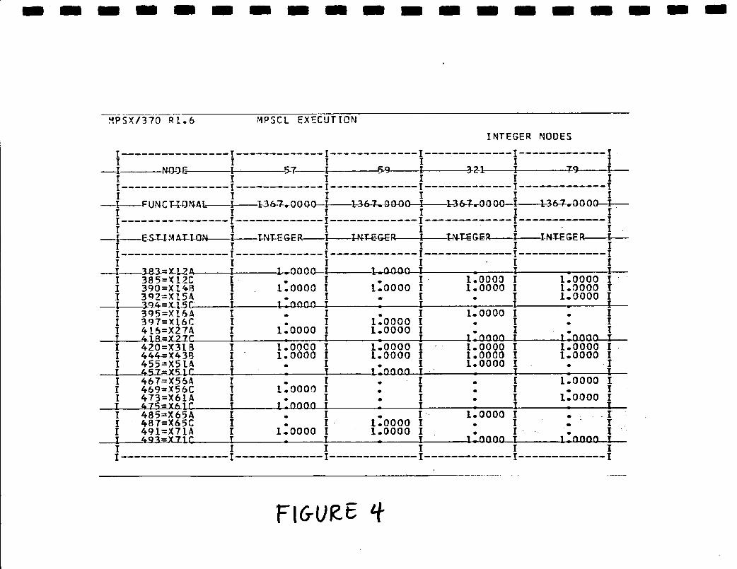
The MIP delivered all six orders with three truck dispatches. The total distance travelled for all three routes was 1376 miles, the optimal integer solution. The first LP solved gave an objective function value of 942 miles.

The total run time for 5706 iterations was 1.37 minutes. (For examples of iterations performed by MPSX and a summary of program results, see figures 3,4,and 5.)

14

PROBLEM SITUATION---"TRUCKS"

We simulated our problem on the TRUCKS software package as closely as possible. We included the same constraints in its system parameters, and "turned off" all other parameters built

into the TRUCKS database that would have given our MIP an unfair

advantage.

We were not, however, able to simulate our model as accurately as we wanted to. TRUCKS' heuristics have assumed two objectives that we did not want: to place a priority on using the largest-capacit y trucks, and to minimize the number of different trucks used.

RESULTS SUMMARY

TRUCKS delivered all six orders with five truck dispatches. The total distance travelled for all five routes was 1476 miles, 100 miles more than the MIP optimum. (See figures 6 and 7 for examples of TRUCKS screens detailing individual route information; see figure 8 for route results summary.)

DETERMINISTIC VS. HEURISTICS

A deterministic solution to a routing and scheduling problem using mixed integer programming gives an optimal solution, clearly defines the constraints, and leaves no room for approximation. However, real-world problems quickly become computationally burdensome. A realistic problem would model a network of hundreds of distribution locations, and would certainly necessitate the inclusion of more complex parameters and constraints than our model did. And the problem matrix increases exponentially with each added variable and constraint. As a result, computer time becomes infeasibly expensive. It is also difficult to simulate real-world situations using linear programming because the real world is not always linear. It becomes impractical to use such MIP solutions in large commercial applications because either a large computer system or expensive rented computer time would be required.

A heuristics-based solution, on the other hand, is much

15

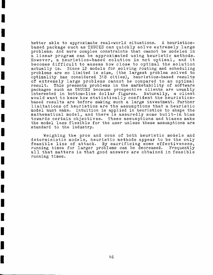
better able to approximate real-world situations . A heuristics-

based package such as TRUCKS can quickly solve extremely large problems. And more complex constraints that cannot be modeled in a linear program can be approximated using heuristic methods. However, a heuristics-based solution is not optimal, and it becomes difficult to assess how close to optimal the solution

dels for solving routing and scheduling actually is. Since LP mo problems are so limited in size, (the largest problem solved to optimality has considered 318 cities), heuristics-based results of extremely large problems cannot be compared to an optimal result. This presents problems in the marketability of software packages such as TRUCKS because prospective clients are usually interested in bottom-line dollar figures. Naturally, a client would want to know how statistically confident the heuristics-based results are before making such a large investment. Further limitations of heuristics are the assumptions that a heuristic model must make. Intuition is applied in heuristics to shape the mathematical model, and there is assuredly some built-in bias towards certain objectives. These assumptions and biases make the model less flexible for the user unless these assumptions are

standard to the industry.

Weighing the pros and cons of both heuristic models and deterministic models, heuristic methods appear to be the only feasible line of attack. By sacrificing some effectiveness, running times for larger problems can be decreased. Frequently all that matters is that good answers are obtained in feasible

running times.

16

Routing and scheduling of vehicles and crews

Table II Characteristic s of routing and scheduling problems.

pOSSIBLE CHARACTUISIICS

OPTIONS

1. Size of Available Fleetone vehicle pltiplC vehicles

homogeneous (only one vehicle type)

2. Type of Available fleetheterogeneous(multiple vehicle types)

ted, etc..) special vehicle types (Co ,aCtsflt

single depot (domicile) 3. liouaing. of Vehicles

multiple depots

deterministic (known) depends

A.. Nature of Depends stochastic depend requirements

asittial sat isfaction of demand alled

S.

Locat ion of Demands on area mixed

undirected

6. tJerl!$ Ne-eyk directed mixed euclidean

imposed (all the same) 7. Vehicle Capacity Restrictions

(different vehicle capacities) imposed(unlimited capacity) not imposed

iosed (aaae for all routes)

g . )UiP'fl b yte Tie" ipoeed (different for different routes).

not imposed

pickups only

9. Operations drop-offs (deliveries) only mixed (pick ups and deliveries)

split deliveries (alloyed or disallowed)

variable or routing colts 10. Costa fixed operating or vehicle acquisition coats

coats (for unaervced depends) Con carrier

.•minimize total routing COStS

sun of fixed and variable costs minimizeU. Objectives minimize number of vehicles rqire4

maximize utility function based on service or cOnVrfltenct

utilitY function baled on customer paxinitepriorities

FI GURE 1

-

rrkQn4

Shrme,odrt

Astin F1 (ri/Re 2.

At%.UI1UN

INVERT - TIME - 1.07 - ITERATTON..4424 -

MIXFIOW - TIME • 1.07 A Afl

• ITER VCTDR VECTOR REDUCED NUMBER FIJNCTIDN NUMBER OUT IN COST NONOPI VALUE D 4500 501 446 00-211 0_L260..-13.l.9._..

INVERT - TIME • 1.09 - ITERATION..4510

MIXFtOW - TIME - I_pg

• INVERT - TIME - 1.09 - ITERATION..4518

I _.flIXF4..ObI.__,._TIJ4E - S*S

ANY FURTHER SOLUTION CANNOT BE BETTER THAN 1130.00 -4-NIIEP T - TIME

MIXFLOW - TIME - 1.11

.-I.N.V-ERT - TIME LII. - I T ERATION 4606

, MIXFLOW - TIME - 1.11 7$

_-ANY FUT.H 40UJ1-I-ON CANNQ-8E_8 JkN I 130.00

2 *** ANY FURTHER SOLUTION CANNOT BE BETTER THAN 1130.00 INVERT —_TIME_•_Ii,_—_ITTTDM..½3

23 MIXFIOW - TIME 2 ANY (JRTW Sfl?1flN ALRE BETTER THAN 113fl-Ofl

*** ANY FURTHER SOLUTION CANNOT BE BETTER THAN 1130.00 -_ Ty"F_-_1.12_-_ITrDAr,flw_65,

MIXFLOW - TIME • 1.12

AN! Eli OLULLO.CANNfILRF BETTER TMA N

INVERT - TIME = 1.13 - ITERATIQN..4686 "_N1XFIflW - TTMF =

—— INTEGER SOLUTION OBTAINED AT NODE 321 AND ITER 4703 - ITS FUNCTIONAL VALUE IS 1367.0000 flflPQTNT flFMANn SET

ER AS

- ESTIMATION OF THE BEST ONE IS 1371.33

- ESTIMATION OF THE BEST ONE IS 1378.10

- ESTIMATION OF THE BEST ONE IS 1389.61

FIGUP,E 3

MPSXI370 R1.6 MPSCL EXECUTIONINTEGER NODES

I ---------------- I-------------I-------------I-------------I------------I I I

—I NL0E 5-7i 5 9 3-21 I 79 I I I I I I I----------------I------I------------1-------------I------------- I I I I I 1 .1

—I FUNCT-IOAL I 1-36-7-.O0OO-T 1367:_.0OOp I 1-36-700 00-I 1364.0000-1---I I I I I I. I ----------------I--------------------------- I--------------I------------I I I I I I I.

—I E-S-1-IMA-T4ON I I-P4-T-EGEl 1—I-N-T-ECE I LN-T-EGER I IN-T-ER I I I I I I I----------------I------------- -I------------- I-----I I I I I

—I 3a3= X1-2 A 1 1 • 0000- h0G0O-I • I I 385=XI2C I • I • 1 1.0000 1 110000 I I 390=X14 I 1.0000 I 1.0000 1 1.0000 1 1.0000 1 I 392=X154 I • I • I • 1 1.0000 1

—1 39.4=X-I-5C I 1.0-000--I • I I I 395=X164 I • I • 1.0000 1 • I I 397=X16C I • I 1.0000 1 I • I I 416=X274 1 1.0000 I 1.0000 1 I • I I_4L8.=X21C_I_•_I_• L0-O.-0-Q.-I_1.0000_1 I 420=X31B I 1.0000 1 1.0000 I 1.0000 I 1.0000 I I 464=X433 I 100000 1 1.0000 I 100000 I 1.0000 I I 455=X514 I • I • 1 100000 I • II 467=X56A I • I . I • 1 1.0000 I I 469=X56C 1 100000 1 • I • I • I I 473=X6IA I • I • I • I 1.0000 1 I 485=X654 I -. I • I 1.0000 I • I I 487=X65C I • I 1.0000 I • I • I I 491=X71A 1 100000 I 1.0000 I • I • I I I I I I -- I

I----------I--,-----------I----- -- ---- I--- --- ------ I

Fl&UP- E If

--_- - -a-. t-.--r-____. - -- -.---------------- o. .___- - -- -

• .... P RO'3LE4 STATISTICS•..COMPUTATIAL ELEMENTS....

Em

ROWS COLUMNS 382

162 F'JNrTTONAL (MIN) RES1'RAINTS 1 C RHS I1TEGEP VARIABLES -544

126 BOUtLDS CI ELEMENTS DENSITY 2506

1.20

r------------I------------ I I I TIME I

TSTNCE MIXSTARTI NODE NO.. I T ERATION NO.1 I FUNCTIONAL ' SINCE SETUP I 1 I I - VALUE I -

I I

_________________________________ 0 I 1 I

I I 920.0000 -- I----------I---------r-- ----- - 1 1 I I FIRST INTEC,ER SOLUTION 1 I L 0.17 I 710 I 57 . I-----------------_ ------- I I - ------------SS_ I 1 I OPTIMA 1 1 L INTEGER SOLUTION 1 0.25 I 1084 1 79 I f

--- I ------______i

I I

1.34 1 5706 I 378 7

378 .. • . I - - ---------___I I - e ee ------

NUMBER OF OF INTEGER VARIABLES NOT INTEGER AT CONTINUOUS OPTIMUM a 14

NUMBER OF INTEGER SOLUTIONS FOUND 4 BRANCHES ABANDONED WHILE COMPUTING a .371 • . . .

F16-UKE 5

I - - -I CONTINUOUS OPTIMUM I

OPTIMALITY PROVED

I ITIME OF SEARCH

- --------I ee - -

1.34 1 5706

1367.0000 1 - -1367.0000

_------ 7.

____.._ __

ute ID...... SAH-1

PLANNED . ute Type...: T (TEAM) tel Dist.... 416 tel Time.... 9:41 ive Time.... 8:20 yover Time.. itTime..... ad/Unload... 1:21

iver 1 ..... iver 2.....: actor ID...: *001*

TRAILER

Last Update.. 05/08/85 *R* Original..... 05/08/85 *R*

ACTUALPlanned Dispatch.. 05/06/85 20:20 Planned Return.... 05/07/85 06:01 Domicile.......... 300-TX

-WGT- -VOL .. •--PCS-- -PAL-Tot Qty 6.0

Max Qty 6.0

-BEG-OD- -END-OD- AUX EQPT --BEG-- --END--

it1..... ..: it2 ....... it3.......

M=HELP 2=TOP 3=EXIT 6=PRINT 9=DELETE 10=BACKWARD 11=FORWARD 12=HONE

- Row 23 Col 6 PROCEED HALF Duplex

UCKS 2.2 ROUTE FILE - GENERAL INFORMATION - SCREEN 1

utA ID...... SAH-2 - - - - Last Update.. 05/08/85 R*

Original..... 05/08/85 *R*

PLANNED Dute Type...: T (TEAM) )tal Diet.... 352 )tal Time.... 9:23 rive Time.... 7:02 yover Time.. it Time..... cad/Unload... 2:21

river 1 ..... river 2 ..... rector ID...: *001*

TRAILER

ACTUALPlanned Dispatch.. 05/09/85 09:59 Planned Return.... 05/09/85 19:22 Domicile.. ... . .. .. 300-TX

-WGT- -VOL- --PCS-- -PAL-Tot Qty 16.0

Max Qty 16.0

-BEG-OD- -END-OD- AUX EQPT --BEG-- --EN!)--

nit 1 ....... nit 2 ....... nit 3.......

> screen F1 = I-iELP 2=TOP 3 = EXIT 6=PRINT 9=DELETE 10=BACKWARD 11-FORWARD 12=HOME

[ Row 23 Col 6 PROCEED HALF Duplex

F1 6-U C E7 G

.1

ID...... SAH-2Last Update.. 05/08/85 *R*

5ute Original..... 05/08/85 "R

CT ---- ARRIVAL --- --- DEPARTURE- - DRIVE LAYOV WAIT LD/UNDIS

0 LOCATION DATE TIME DATE TIME TIME TIME TIME TIME

-- 1 - 300-TX 05/09/85 09:59 05/09/85 10:29 :30

1:36 176 2 - 328-AR 05/09/85 14:00 05/09/85 15:3 6 3:31

:15 176 3 - 300-TX 05/09/85 19:07 05/09/85 19:2 2 3:31

?F1=HELP 2=TOP 3=EXIT 4=REROUTE 5=SELECT 6=PRINT 7=UP 8=DOWN 9=DELETE HALF Duplex

Row 23 Col 6 PROCEED

rRUCKS 2.2 ROUTE FILE - STOP SUMMARY -'SCREEN 2 PAUE 01 OF 01

Last Updat 05/08/85 * R* Route ID SAH-3 Original..... 05/08/85 **

AC ---- ARRIVAL --- --- DEPARTURE- - DRIVE LAYOV WAIT LD/UN TIME DIS

NO LOCATION DATE TIME DATE TIME TIME TIME TIME

01 - 300-TX 05/08/85 06:54 05/08/ 8 5 07:24 :30 1:48 90 j

02 - 316-TX 05/08/85 09:12 05/08/85 11:00 1:48:31 :36 99

03 - 324-LA 05/08/85 13:30 05/08/85 14:06 1:59:15 189

04 - 300-TX 05/08/85 17:53 05/08/85 18:08 3:47

PF1=HELP 2=TOP 3=EXIT 4=REROUTE 5=SELECT 6=PRINT 7=UP 8DOWN PROCEED

9=DELETE HALF Duplex

Row 23 Col 6

TRUCKS 2.2 ROUTE FILE - STOP SUMMARY - SCREEN 2 PAGE 01 OF 01

Last Update.. 05/08/85 *R* Route ID...... SAH-4 Original .....05/08/85 *R*

ACT ---- ARRIVAL --- --- DEPARTURE- - DRIVE LAYOV WAIT LD/UN TIME TIME DIS

NO LOCATION DATE TIME DATE TIME TIME TIME

01 - 300-TX 05/06/85 12;;2 05/0/85 13:02 :30 1:12 48

02 - 308-TX 05/06/85 14:00 05/0 6 / 8 5 15: 12 :58:15 48

03 - 300-TX 05/06/85 16:10 05/06/85 16:25 :58

FIGzUPE.

DOMICILE STRING ROUTE TYPE DISPATCH RETURN DRIV

--------- -- -

300-TX 001 SAH-4 T 05/06/85 13:3 2 05/06/85 17:25 1:5

300-TX 001 SAH-1 T 05/06/85 21:20 05/07/85 07:01 8:2

L 300-TX 001 SAH-3 T 05/08/85 07:54 05/08/85 19:08 7:3

1 300-TX001 SAH-^ T 05/09/85 10:59 05/09/85 20:22 .7:0

300-TX 002 SAH-5 T 05/08/85 06:09 05/08/85 13:24 4:4

IREPORT NO: TK-501TEST COMPANY, ROUTER LOG FOR

INC. ROUTE GROUP: SA

I DATE/TIME: 05 1/ 081/ 85 19:59TRACTOR USAGE SUMMARY

NON-SLEEPER SLEEPER

DOMICILE POOL USED POOL USED

11 A[ Row- - 2- - Col- - 7PROCEED HALF Duplex

ROUTER LOG Al F 131 3 BLKS 85/05/08 LINE 60 OF 82 BROWSE I

ORDERSINPUT...... . . ... ... ..... .1..: 6 1 ORDER FREQUENCIES INPUT. ...........: 6 ORDERS THAT FAILED TO BE ROUTED....: 0

ORDER FREQUENCIES THAT FAILED ......: 0

II

LOCATION RECORDS IN THE DATABASE...: 90 DOMICILE LOCATIONS ......... . . . . . . . .: 1

LOCAL ROUTES GENERATED... ..........: 0 SMOTR ROUTES GENERATED............: 0 TEAM ROUTES GENERATED... : ..........: 5

I

TOTAL ROUTES GENERATED.............: 5

TOTALDRI VE TIME... .... ... .... .. ...: 29:34 TOTAL LAYOVER TIME. . . . . . . .... . . .

' TOTAL WAIT TIME........... .........: :31 TOTAL LOAD/UNLOAD TIME.............: 11:21

I

TOTAL ROUTE TIME .......... :41:26

TOTAL ROUTE DISTANCE ...............:1476

I .....

II

BIBLIOGRAPHY

:1. L. Bodiri, B. Golden, A. Assad, and M. Ball, COMPUTERS & OPERATIONS RESEARCH, SPECIAL ISSUE: ROUTING AND SCHEDULING OF VEHICLES AND CREWS, THE STATE OF THE ART. Vol. 10, no. 2, pp. 63-211, 1983.

2. ST:E.:,:: user "s guide for TRIJI::F::s

:3.

J. Y ':' urp q , "The PC: Masters the Route Between Truck Stops",

PC: MAGAZINE, August, 1984, pp. 220-223.

4. Nand Lal Singh, "The Coming Wave In Vehicle Routing and Scheduling : A Step-By-Step Approach", THE PRIVATE

CARRIER, November, 1984, pp. 10-12.

IL 1

S..,

.4%% 4;? - ^/& AW-00 IrA4Z el-aw 4e4v-.-,

óot a z4 ,"1i 6L I/*4 e /

,jL

/ — I

• /

4(t jzz/

3 2J'L

0

ite-Ia'ery t•a

(r ty p /CefaL i' 17)

ta4 ^(oriu)

uk e7Mie

.N

,- 1 14-+tV n$ * tci/es e I' U I A

Ttkc

aAA 5ckd(411

.

1p.&fl KI

f

'I-/

1 Li

Y

levn

C

I I 1 I I

OPTIMIZATION VS. HEURISTIC

METHODS FOR VEHICLE

ROUTING AND SCHEDULING PROBLEMS

IChristi Hale

Sharon Hatcher I I I I I

for

I OREM 4390, SENIOR DESIGN

May, 1985

ri

Li I LI I

ACKNOWLEDGEMENTS

We wish to thank STSC, Inc., of Rockville, Maryland, I for their generous support of this project. In particular, we thank Mr. Nanlal Singh for initiating this idea and his encouragement throughout. I

DETERMINISTIC VS. HEURISTIC METHODS FOR SOLVING VEHICLE ROUTING AND SCHEDULING PROBLEMS

Distribution costs add about $400 billion each year to the cost of purchased goods in the U.S. alone. The costs associated with operating vehicles and crews for delivery purposes form an important component of total distribution costs. Therefore, even small percentage savings in these expenses could result in substantial total savings over a number of years. And in an increasingly technological society which must take advantage of economies of scale, the relative importance of transportation will continue to grow, and thus routing and scheduling applications will increase in importance.

"Routing and Scheduling" problems refer to the effective management of a fleet of vehicles and associated crews. Private firms that undertake the distribution of their goods to customer locations, and public transportation authorities responsible for providing transportation services to users both rely on routing and scheduling. "Routing problems" give solutions concerning the spatial configuration of vehicle movements, and these problems usually specify a sequence of locations that a vehicle must visit. "Scheduling problems" explicitly consider the times at which various locations are visited. However, in many instances the spatial and temporal characteristics interact and result in "combined routing and scheduling" problems.

An extensive list of applications of routing and scheduling models include mass transit scheduling of vehicles and crews, pick-up and delivery distribution systems, design of dial-a-ride systems, and school-bus routing and scheduling. The area of routing and scheduling has recently been the focus of intensive research activity. Major advances in this area have been made along both theoretical and applied dimensions.

CLASSIFICATION OF ROUTING AND SCHEDULING PROBLEMS

Basically, the output of all routing and scheduling problems is the same. For each vehicle, a route and a schedule is produced. In general, the route specifies the order that each location will be visited and the schedule designates the times at which the activities at these locations are to be performed.

However, routing and scheduling problems may be classified into one of three major groups: routing, scheduling, or combined

routing and scheduling. Combined routing and scheduling problems may be further subdivided according to a more detailed classification system. Each particular problem is distinguished by characteristics and assumptions that pertain to the given situation. The characteristics, restrictions, and assumptions associated with each problem result in different categories of problems requiring different modeling assumptions. For example, figure 1 (1, P. 73) reveals various combinations of options for eleven characteristics of routing and scheduling problems. Each combination of these various options would result in a problem with unique characteristics.

COMPLEXITY OF ROUTING AND SCHEDULING PROBLEMS

In the formulation and solution of Routing and Scheduling problems, it is important to consider the computational burden associated with various solution techniques. The growth in computation time clearly increases as a function of problem size. In a realistic environment where typical routing and scheduling problemsare extremely large, the computation time is prohibitive. Therefore, the applicability of some solution techniques is extremely limited in real-world application.

Since the computational burden in solving these problems grows almost exponentially with problem size, methods of approximation are often resorted to as an alternative to pursuing an optimal solution. The use of heuristics allows for a near-optimal solution. "A heuristic algorithm is a procedure that uses the problem structure in a mathematical (and usually intuitive) way to provide feasible or near-optimal solutions. A heuristic is considered effective if the solutions it provides are consistently close to the optimal solution." (1, P. 76) A powerful heuristic method is defined on the basis of the statistical distribution of answers produced over a range of problems.

EXAMPLES OF HEURISTICS METHODS

A variety of heuristic approaches have found wide use. Here we describe two routing problems and heuristic procedures that have been developed to aid in obtaining near optimal solutions for each type.

2

TRAVELING SALESMAN PROBLEM

The traveling salesman problem determines the minimal cost cycle that passes through each node in a network exactly once.

"Clark and Wright Savings" Method: a heuristic approach to constuct a tour in a traveling salesman problem.

(1) select any node as the central depot (denoted as

(2) compute savings S;,. = C. + C,1 - for i,j =2,3,..,n.

(3) order the savings from largest to smallest. (4) begin at the top of the savings list and move

downwards, forming larger subtours by linking appropriate nodes i and j. Repeat until a tour is formed.

VEHICLE ROUTING PROBLEM

The vehicle routing problem requires a set of delivery routes from a central depot to various demand centers, each having service requirements, in order to minimize the total distance covered by the entire fleet. The vehicles have specified capacities, and each starts and terminates at the central depot. Two heuristic solution stratgies for vehicle routing problems are the "cluster first-route second" approach, and the "route first-cluster second" approach.

"Cluster First-Route Second" Approach: groups demand nodes and arcs first and then designs economical routes over each cluster as a second step.

"Route First-Cluster Second" Approach: works in reverse. A large, and usually infeasible route is constructed which includes all nodes and arcs. Then the large route is partitioned into a number of smaller, feasible routes.

OTHER HEURISTICS (1, P. 99)

MATHEMATICAL PROGRAMMING APPROACHES are based on mathematical programming formulations for the problem.

INTERACTIVE OPTIMIZATION is a general-purpose approach in which a high degree of human interaction is

3

incorporated into the problem solving process. The idea is that experienced decision-makers have the capability of setting the revising parameters and injecting subjective assessments based on knowledge and intuition into the optimization model.

THE AVAILABLE TECHNOLOGY TO SOLVE VEHICLE ROUTING AND SCHEDULING PROBLEMS IN COMMERCIAL APPLICATIONS

Until recently, only the larger companies have been able to utilize computer systems in the distribution area. These systems were very effective, but they were expensive to design and maintain. Most of these systems were individually designed and implemented for particular companies, and demanded expensive, on-going, in-house support.

However, with advancing computer technology, smaller, more affordable computers have been designed to meet the needs of smaller companies. Off-the-shelf computer programs currently exist and are less expensive, simpler, and do not demand professional in-house support. These developments have made automated distribution systems feasible for companies of all sizes.

Various software packages designed for the PC help companies solve distribution problems. For example, ROUTEMASTER, offered by Applied Operations Research, Inc., lists for approximately $200. It optimizes the sequence of stops in a single truck route, minimizing time or mileage, and cost. However, ROUTEMASTER is not as intelligent as some other packages, and it ignores several important variables. A more complex package is TRUCKSTOPS offered by MicroAnalytics for a little over $900. Although TRUCKSTOPS is more expensive, it is also much more intelligent. This package designs a route for each truck and sequences the stops on that route to minimize the total route cost in terms of mileage, time, and overtime.

TRUCKS, offered by STSC, is perhaps one of the most complex and intelligent of the software packages available for solving routing and scheduling problems. This remarkable package is used by companies such as Frito-Lay, Safeway, and Martin-Brower, which services McDonald's. TRUCKS sells for approximately $175,000. The package is heuristics-based, but it takes into consideration almost any constraining condition imaginable. The system parameters that have a significant influence on the routing

operation of the package are listed and described below. (2, pp. 631-641) These parameters are divided into three groups according to the level of importance in the routing operation. Type A constraints are the most fundamental to model, Type B constraints are somewhat difficult to model and moderate in importance, and Type C constraints are the most luxurious and the most difficult to model. And some constraints range from Type A to Type C depending on the complexities involved.

TYPE A CONSTRAINTS

MAXIMUM ROUTE ON-DUTY-TIME This constraint limits

on duty. On-duty time is the (pre-trip and post-trip), all drive time. In our model we time to a 48-hour maximum.

the number of hours a driver may be sum of all load and unload times, driver wait times, and total route limit each driving team's on-duty

MAXIMUM ROUTE DISTANCE This constraint limits the total distance of any single

route. In our model we put a different limit on each route. We limit route A to 500 miles, route B to 600 miles, and route C to 450 miles.

SERVICE TIME AT EACH LOCATION This constraint limits the service time at each stop along a

route, and is based on some base unload rate multiplied by the quantity unloaded. Our model assumes the base unload rate is six minutes/pallet, which converts to 0.10 hour/pallet. Multiply the unload rate by the quantity unloaded to obtain the service time at each location.

PRE-TRIP TIME This time is actually considered part of a route. It is the

time at the beginning of a route that accounts for administrative overhead, equipment inspections, etc. Our model assumes pre-trip time to be 30 minutes.

POST-TRIP TIME This time is also considered part of a route. It is the

time at the end of a route allocated for a driver to end a route. Our model assumes post-trip time is 15 minutes.

LENGTH OF ROUTING CYCLE This constraint limits the length of time within which all

vehicles used in the routing cycle must be dispatched and returned. Our model assumes the maximum length of the routing cycle to be five days.

I MAXIMUM STOPS PER ROUTE This constraint sets a maximum number of stops allowed for each route. The constraint is used to control the maximum size I of any route generated. The domicile stop at each end of the route is included in the number of stops in a route. Our model sets a maximum of three stops per route.

I MAXIMUM ORDERS PER ROUTE This constraint sets a maximum number of orders allowed for a single route. Our model assumes that an order equals a stop. Therefore, there is a maximum of three stops per route also.

- LOCATION WINDOWS These constraints limit the times that a particular location I is open to receive an order. This window applies to all orders

picked up or delivered at a particular location. For example, location X is open to receive orders only from 6 a.m. to 8 a.m. every day.

ASSIGNED DOMICILE

I

A specific domicile (or central depot) can be assigned to certain distribution areas. This forces these distribution areas to be serviced by vehicles originating only from the designated domicile. Our model assumes that one domicile

I(Dallas) services six customers.

TYPE B CONSTRAINTS

CAPACITY VS. TRAILER TYPE Our model assumes one unit of measure for the loads

(pallets) as opposed to multiple units of measure (weight, volume, pallets). Our model assumes that we have multiple trailer types each with a different capacity. The capacity of vehicle A is 30 palettes, vehicle B is 40 palettes, and vehicle C is 25 palettes.

MAXIMUM CAPACITY PERCENTAGE or MAXIMUM TRAILER LOAD This constraint limits the capacity on each vehicle during a

route. The capacity of the vehicle type is considered when determining the total load on a trailer as stops are added -to the route. We assume that all three vehicles are only loaded to 90 percent capacity. Therefore the maximum load on vehicle A is 27 palettes, on vehicle B it is 36 palettes, and on vehicle C it is 22 palettes.

MAXIMUM SHIFT TIME This constraint limits the maximum number of on-duty hours

(including pre-trip time, post-trip time, load and unload times, and driver wait times) a driver may have before a lay-over is required. This constraint applies only to domicile locations and restricts shift times for routes run from that domicile.

MAXIMUM DRIVE TIME This constraint limits the maximum number of driving hours

only before a lay-over is required. This constraint also applies only to domicile locations and restricts drive times for routes run from that domicile.

MAXIMUM WAIT TIME AT A STOP This constraint limits the amount of time a vehicle may wait

at a location before the time windows are open. Wait time provides some flexibility, especially when time windows tend to be very tight. Our model assumes that maximum wait time at a stop must not exceed four hours.

MAXIMUM TOTAL WAIT TIME IN A ROUTE This constraint limits the total sum of all wait times for

all stops in a route.

MAXIMUM ROUTES AVAILABLE This constraint limits the maximum number of routes that may

be dispatched in a given time period.

ORDER WINDOWS This constraint specifies the earliest and latest pick-up

and delivery dates and times allowed for each order. Order windows are used to further restrict the handling of an order because they restrict the time a particular order is handled at a location.

TYPE C CONSTRAINTS

I ORDER WANDER LIMIT The order wander measures for each step the ratio between a particular route distance and a direct line distance from the I route origin. A low ratio acts as a limit on the amount of "wandering" the Router can do to fit new routes into the schedule.

I ROUTE WANDER LIMIT The route wander measures for each stop the ratio between the total route distance developed so far and the minimum route I

distance to service the orders. The ratio helps keep a route from crossing over itself and increasing mileage.

11

MINIMUM DISTANCE FOR SMOTR/TEAM ROUTES This constraint limits the total route distance before a

route will be considered no longer a "local" route, but a single-man-over-the-road (SMOTR) route or a team route.

SINGLE-TO-TEAM CUTOVER TIME The cutover time constrains the maximum allowable length of

a route run by a single driver, ignoring the length of a shift. Once a route is no longer considered "local" and has been assigned as a SMOTR, if the single-to-team cutover time limit is exceeded, the route is considered for assignment to a team.

SINGLE-TO-TEAM CUTOVER DISTANCE

I

If either the single-to-team cutover time limit or the single-to-team cutover distance limit is exceeded, the SMOTR will become a team.

I ADDITIONAL CAPACITY PERCENTAGE This parameter measures how much more capacity a trailer can have during a route if it is not already empty. It permits I

control over the amount of cargo shifting necessary during a route with mixed pick-up and deliveries.

MINIMUM REDISPATCH TIME I This constraint sets the time to be allowed unscheduled between successive dispatches of the same vehicle and driver. This constraint does not include the time at the domicile.

BASE COST MARGIN The base cost for an order is calculated for each available

domicile based on that domicile's stated equipment cost per mile and the distance necessary to service the order. Any domicile whose base cost falls outside this limit will not be considered as a domicile for this order. This margin allows the router to choose a suitable domicile to service a set of orders in a multiple domicile situation. This constraint would not apply to our model since we assume a single assigned domicile.

ROUTING CYCLE OVERLAP Routing cycle overlap allows a route to be dispatched in one cycle and return in the next cycle as long as the total route length plus any redispatch time requirement does not exceed the length of one full cycle.

MINIMUM LAYOVER This constraint sets a minimum on the amount of lay-over

time of routes originating at the corresponding domicile location.

8

MAXIMUM LAYOVER This constraint sets a maximum on the above.

TIME ZONES This parameter takes into account the fact that routes may

cross into different time zones. This constraint would not apply to our model since we are routing only through the Texas, Louisianna, Arkansas, Oklahoma areas.

PRODUCT CLASS VS. TRAILER TYPE The product class of an order must be compatible with the

classes of other orders on the same trailer. This constraint would not apply to our model since we assume only a single product class, OR1.

ORDER FREQUENCY AND MINIMUM SPACING Order frequency is the number of times the order is to be

serviced in a single routing cycle, and the spacing is the minimum time to be allotted between deliveries. This creates multiple duplicate orders of the same kind.

RANGES OF CONSTRAINT TYPES

Some of the Type A constraints may range to Type B and Type C constraints with added complexities.

LOCATION WINDOWS A Type A constraint on location windows assumes that there

is one window open to receive an order at the same time each day. However, a Type B constraint would occur with multiple windows open any day, and a Type C constraint would occur with multiple windows open only on specific days.

CAPACITY VS. TRAILER TYPE Our constraint is a Type B. We assume one unit of measure

(pallets, and multiple trailer types. A simpler Type A constraint would assume one unit of measure and one trailer type, while a more complex Type C constraint would assume multiple units of measure and multiple trailer types.

DOMICILE Our model assumes the Type A constraint that we have a

single domicile. However, a more complex Type B or C constraint could assume multiple domicile locations.

SERVICE TIME AT EACH LOCATION Our model's Type B constraint assumes the service time is

I determined by the set unload rate multiplied by the quantity unloaded. A simpler Type A constraint would assume a base unload time not related to the quantity unloaded. A more complex Type C constraint would assume various unload rates for various product

Iclasses at various delivery locations.

OBJECTIVE FUNCTION Our model assumes a Type A objective function that we

I minimize cost (with cost in terms of miles). More complex objective functions would result if we minimized more than one variable type. For example, we could minimize cost or miles, hours, and I number of vehicles required, all in the same objective function.

IOUR MIXED INTEGER PROGRAMMING MODEL

I

Our simplified model of a routing and scheduling problem is based on a distribution network with one central depot which distributes goods to a large region. The input data is a set of orders from six customers during one business week. (See figure I 2) The distribution center has three trucks available to make deliveries, each with a different capacity and route-mileage limit.

In the model, we formulated first what we believed to be the most fundamental constraints, such as the miximum distance each truck can travel, and "subtouring" constraints to insure that the trucks return home to the central depot. With that accomplished, we sought to add constraints which would be valuable in making our model simulate a real-world situation. Our choice was limited by the fact that we were programming in LINDO, which processes a maximum of 400 constraints. The most dificult but necessary constraint of those we chose was the arrival-time constraint, which forces delivery to occur within a time interval specified by the customer. This feature alone represents over 200 constraints in the mixed integer program; over half of the total number of constraints.

An example of a feature we did not include because of the complexity it would add to the model is a maximum-number-orders for trucks' routes. We assume in our model that one stop is equivalent to one order, but in a real-world situation, one stop may have multiple orders. Another example is having both location windows and delivery windows; our model is limited to one set of windows.

10

The variables, constants, and assumptions of the model are as follows:

VARIABLES

0-1 integer variable representing an arc from node (customer) i to node j for truck v. For seven nodes (one depot and six customers) and three trucks, there are 126 X v 's.

Aj Arrival time at node j; Aj represents arrival time at the previous node 1.

VWait time at node j for truck v.

Ut, U3 Variables associated with nodes i and j, employed in the subtouting-elimination constraints.

CONSTRAINT PARAMETERS

n 7 : Number of nodes.

V = 3 : Number of vehicles (trucks) available.

C = Capacity of truck V in pallets. C, = 30, C, = 40, C3 = 25

P = 90 : Percent loading capacity of each truck, effectively making C, = 27, C 2 = 36, C3 = 22.

= Demand (quantity ordered) at node ± in pallets. q, =0 qE=6 q3 =12 q 6 16 q 3 -18 q=6

= 18

dJ = Distance from node ± to node j in miles.

= Maximum route distance for truck v. = 500, D . = 600, D = 450

T = 48 : Maximum route-time allowed in hours.

= 0.5 (30 minutes): pre-trip time for each route.

t pøsr = 0.25 (15 minutes): post-trip time for each route.

A = Earliest delivery date/hour for each node j.

1 Aj = Latest delivery time for node j.

ASSUMPTIONS

1) The product being delivered is homogeneous; it is the same for all customers.

2) The product is unloaded at a constant rate. We assume 10 pallets per hour.

3) The trucks' travelling speeds are the same, and assumed to be 50 mph.

4) All deliveries take place within a time-frame of five consecutive days (one business week).

5) Team drivers are used, so that many single-driver work-rules (i.e. 8-hour shift limit) can be disregarded.

MATHEMATICAL FORMULATION

The mathematical formulation of the mixed integer program involves ten basic constraints, which expand to 388 constraints when coded.

OBJECTIVE FUNCTION: v MINIMIZE Z ZZ dij x

(minimize total distance travelled to make all deliveries)

Such That:

n

1) x I (i = 2,...,n) LI YI

tjX j 1 (i = -V7 ̂ ='

teach customer must be serviced by one truck)

12

H I fri

2)

I p i'j (v = I p = 1,...,n5

(route continuity must be preserved; i.e. if I a truck visits customer i, it must leave customer i)

1 3)q (x) C, (v =

(the trucks' capacities cannot be exceeded I for deliveries on an assigned route)

I x (v

(maximum route distance for each truck cannot

Ibe exceeded)

I 11 h

Zo.ioq(Zx) + 0. 02 dj <1^

T- pE (v =

Assuming unload rate = 6 mm/pallet,

Idriving speed = 50 mph. ( total route-time must not exceed maximum T)

I 6) 1d "'J J (j =

I (arrival time must fall within window specified by customer)

I )(V_ 3 (v = t= t ji J (maximum number of stops per route is 3)

8) AS(AL+o.Io oz+ J)- (i-x,)T I (& 0. 1 0,02d, W, I I

for all i,j,v (arrival time formulation)

I 13

F,

9)4(j = 2,...,n

j v =

(maximum wait-time at a customer stop is 4 hours)

10) tA — UJ ± V) Xo V

il — I

i =2,...,n; j = 2,...,n; v =

(subtours are not truck must return route completion)

allowed; truck must to central depot for

PROBLEM SOLUTION --- MIP

When we attempted to run our program on LINDO, we found that although we had stayed within the limits for the total number of constraints and variables, it could not solve the problem. The obstacle was our 126 integer variables. Although LINDO has a capacity of 599 variables, it cannot handle nearly as many integer variables.

Our alternative was to solve the problem on the MPSX (Mathematical Programming System) package on the IBM computer. LINDO has a feature to convert a mixed integer problem to the MPS input format required. After converting our problem, MPS was able to solve it successfully.

RESULT SUMMARY

The MIP delivered all six orders with three truck dispatches. The total distance travelled for all three routes was 1376 miles, the optimal integer solution. The first LP solved gave an objective function value of 942 miles.

The total run time for 5706 iterations was 1.37 minutes. (For examples of iterations performed by MPSX and a summary of program results, see figures 3,4,and 5.)

1 14

PROBLEM SITUATION---"TRUCKS"

I

We simulated our problem on the TRUCKS software package as closely as possible. We included the same constraints in its system parameters, and "turned off" all other parameters built into the TRUCKS database that would have given our MIP an unfair

Iadvantage.

We were not, however, able to simulate our model as accurately as we wanted to. TRUCKS' heuristics have assumed two objectives that we did not want: to place a priority on using the largest-capacity trucks, and to minimize the number of different trucks used.

RESULTS SUMMARY

I TRUCKS delivered all six orders with five truck dispatches. The total distance travelled for all five routes was 1476 miles, I 100 miles more than the MIP optimum. (See figures 6 and 7 for examples of TRUCKS screens detailing individual route information; see figure 8 for route results summary.)

DETERMINISTIC VS. HEURISTICS

A deterministic solution to a routing and scheduling problem using mixed integer programming gives an optimal solution, clearly defines the constraints, and leaves no room for approximation. However, real-world problems quickly become computationally burdensome. A realistic problem would model a network of hundreds of distribution locations, and would certainly necessitate the inclusion of more complex parameters and constraints than our model did. And the problem matrix increases exponentially with each added variable and constraint. As a result, computer time becomes infeasibly expensive. It is also difficult to simulate real-world situations using linear programming because the real world is not always linear. It becomes impractical to use such MIP solutions in large commercial applications because either a large computer system or expensive rented computer time would be required.

A heuristics-based solution, on the other hand, is much

15

better able to approximate real-world situations. A heuristics-based package such as TRUCKS can quickly solve extremely large problems. And more complex constraints that cannot be modeled in a linear program can be approximated using heuristic methods. However, a heuristics-based solution is not optimal, and it becomes difficult to assess how close to optimal the solution actually is. Since LP models for solving routing and scheduling problems are so limited in size, (the largest problem solved to optimality has considered 318 cities), heuristics-based results of extremely large problems cannot be compared to an optimal result. This presents problems in the marketability of software packages such as TRUCKS because prospective clients are usually interested in bottom-line dollar figures. Naturally, a client would want to know how statistically confident the heuristics-based results are before making such a large investment. Further limitations of heuristics are the assumptions that a heuristic model must make. Intuition is applied in heuristics to shape the mathematical model, and there is assuredly some built-in bias towards certain objectives. These assumptions and biases make the model less flexible for the user unless these assumptions are standard to the industry.

Weighing the pros and cons of both heuristic models and deterministic models, heuristic methods appear to be the only feasible line of attack. By sacrificing some effectiveness, running times for larger problems can be decreased. Frequently all that matters is that good answers are obtained in feasible running times.

16

Routing and scheduling of vehicles and crews

Table I.I. Characteristics of routing and scheduling problems.

QARACRISTICS POSSIBLE OPTIONS

1. Size of Available fleet one vehicle

multiple vehicles

homogeneous (only one vehicle type) 2. Type of Available Fleet heterogeneous (multiple vehicle types)

special vehicle types (compartmentalized, etc.)

3. Housing of Vehicles single depot (domicile)

multiple depots

deterministic (known) demands A. Nature of Demands stochastic demand requirements

nartial satisfaction of demand allowed

at nodes (not necessarily all)

5. Location of Demands an area

mixed

undirected

6. Underlying Network directed

mixed

euclidean

7. Vehicle Capacity Restrictions imposed (all the same)

Imposed (different vehicle capacities)

not imposed (unlimited capacity)

imposed (lame for all routes) S. Maximum Route Times

imposed (different for differeot routes).

not imposed

pi'ckups only 9. Operations drop-offs (deliveries) only

mixed (pick ups and deliveries)

split deliveries (allowed or disallowed)

10. Coats variable or routing costs

fixed operating or vehicle acquisition coats

con carrier coats (for unserviced demands)

minimize total routing coats 11. Objectives minimize sun of fixed and variable costs

minimize number of vehicles require,

maximize utility function based on service

or convenience.

maximize utility function based on customer

priorities

FIGURE 1

O.t4*1m4 &fr,Có'5 rd1f 6W

,q440

7êrar-kz'n4

Shraee,00rt

4ustin Fl(ruge 2.

• MP$X/370 R1.6 MPSCL EXECUTION PAGE 16 85/126 INVERT - TIME = 1.07 - ITERATION..4424 MIXFLOW - TIME 1.07

ANY -__.STfiqA 8—BE S7—ONE I S 1-364.74 ITEP VCTOR VECTOR REDUCED NUMBER FUNCTION NUMBER OUT IN NUMBER SUM COST NONOPT VALUE 0 45.00 507 INFEAS INFEAS 446 00211 0 1260.7'479-

INVERT - TIME = 1.09 - ITERATION..4510 6 —MI-XE-LOW - TIME

INVERT - TIME = 1.09 - TTERATION..4518 J4IXE-L.OWS-__S_ST.TME —1-,.-09-

*** ANY FURTHER SOLUTION CANNOT BE BETTER THAN 1130.00 - - ESTIMATION OF THE BEST ONE IS 1371.33 —I-NVEPT - TIME 1_jo - I-E-R.47-Z-Qri__4578

MIXFLOW - TIME = 1.11 - TIME = LII - XTEPTI0114606

MIXFLOW - TIME • 1.11 — A NX Eu* 074 E—-T-ER4HA4 1130.00 - 8 ST- 3N—OE_7HE ES-T_-ONE

2 *** ANY FURTHER SOLUTION CANNOT BE BETTER THAN 1130.00 2 1 INVERT - TI ME = - ITERATION .463

- ESTIMATION OF THE BEST ONE IS IS1..3-78..4O

1378.10

23 M!XFLOW - TIME 1.12 2 ** AMY URTHR S flL!JT TflM C A NNflI_RE BETTER TH A N nfl jj3fl - c5TMATjTi fl T'E357_QNE IS 135B.Qp

*** ANY FURTHER SOLUTION CANNOT BE BETTER THAN 1130.00 _1N!FPT - TTMF = 1I - YTRArTflN.4Ac,

- ESTIMATION OF THE BEST ONE IS 1389.61

;: MIXFLOW - TIME • 1.12 ° __S**_ANY CjJRflJ.SflLU71ONfff__RF R ETT ELX1 A M lIlfl_flfl FcTTMAflON flc TH_.35T ONE Tc 1403.19

INVERT - TIME = 1.13 - ITERATION..4696 .MIXFJ..flW - TI MF = I I

3! INTEGER SOLUTION OBTAINED AT NODE 321 _X.DOPOI NT TIFMANfl SFT

AND ITER 4703 - ITS FUNCTIONAL VALUE IS 1367.0000 31

39

3,

FIGUZE 3

- - - - - - - - - - - - - - - - -

MPSX/370 R1.6 MPSCL EXECUTIONINTEGER NODES

I----------------- I------------- -------------- I -------------I ------------- I I I I I I

-I N0-0-E I 5-7 5-9 3-2-1 1 79 I I I I I I I----------------I----- ------1-------------I-------.-------I I I I I I I i FUNCT4OM-AL_I1-36-7-.O00O_I1-36-7-.-00-0O_I1-36-7-.0000-I 136-7-.0-00--4-----

I I I I r I----------------I------------- I------------- I--------------I-----------I I I I I I I.

-I-E-S-T-I. MAX-1-ON_I_IT-EGE-R -T-E.GER_I_I-N-T-EGER I IN-T-ECE-R_I I I I I

I----------------I-------------I------------- I-----I I I I

-1 383= X-1-2 A_1 • 0(O- 10-3- 385=X12C I • I • 1 1.0000 1 1.0000 I

390=X14 I 1.0000 I 1.0000 1 1.0000 I 1.0000 I I 392=X15A I . 1 • I • I 1.0000 1

-I )c)-4=X-1-5C 1-1-.-0-O0-0---I_•__•__I 395=X16A I . . 1 1.0000 I

• I• I

I 397=X16C I 416=X274

I I

• 1.0000 1

1.0000 I 1.0000 I • I

• • I

- 418-X22C • I a I 1..00G0_I 1.0000 I I 420=X313 I 1.0000 1 1.0000 1 1.0000 I 1.0000 I

444=X433 I 1.0000 I 1.0000 I 1.0000 I 1.0000 I I 455=X514 1 • I • I 1.0000 I • II 467=X554 I • I • I • 1 1.0000 I I 469=X56C I 1.0000 1 • I • I • I I 473=X6IA I • I • I • I 1.0000 I I 485=X65A I• I • I 1.0000 I • I 487=X65C I • I 1.0000 I • I • I 491=X71A I 1.0000 I 1.0000 I • I •

I - I - I - I I--------------I------------I-----

&ugE Lj.

STATISTICS ..... ...COMPUTATI34AL ELEMENTS....

ROWS 382 F'JNrTIONAL (MIN) 1. C COLUMNS .162 RES1'RAINTS RHS CI VARIABLES 5.44 ROUNDS -I r TEGER. VARIABLES 126 ELEMENTS 2506 DENSITY 1.20

I-------------------------I --------------I------------- i --------I I TIME I ITERATION N0.1 NODE NO.. I FUNCTIONAL I I ISTNCE M IXSTARTISINCE SETUP I I VALUE I

I 1' 1 r I. I ---------- I-------------- I -------------- I------------j -----_-------I-I I - t -V - I I I I CONTINUOUS OPTIMUM I . • I . 0 I 1 I 920.0000 I I I----------- - -I-------------I . I I . I I I FIRST INTEGER SOLUTION 1 0.17 I 710 I 57 1 1367.0000 1 _.t . . I I I---------------I--------------E-------------i--------

I 1 1 1 I I I OPTIMAL INTEGER SOLUTION I 0.25 I 1084 I 79 1 1367.0000 I I I I I -----------------I-------------I----------•--I----------------.I----------I. I I I I I I I OPTIMALITY PROVED I 1.34 1 5706 I 378 I I I----------------1---------------I------------1------------I-------------I.

V I I I I • .1 I I TIME OF SEARCH 1 1.34 I 5706

.

378 I . .1 I----------------.-----I--,--.----------I----------------

NUMBER OF INTEGER VARIABLES NOT INTEGER AT CONTINUOUS OPTIMUM = 14 NUMBER OF INTEGER SOLUTIONS FOUND = 4 BRANCHES ABANDONED WHILE COMPUTING = .371'

F16-UKE 5_

IRoute ID. SAH-1 Last Update.. 05/08/85 *R*

Original..... 05/0;/85 *R* PLANNED ACTUAL

Route Type...: T (TEAM) Planned Dispatch 05/06/85 20:20 Total Dist 416 Planned Return.... 05/07/85 0601 Total Time .... 9:41 Domicile ..........300-TX

Time 8:20

I

Drive Layover Time -WGT- -VOL- --PCS-- -PAL-Wait Time Tot Qty 6.0 Load/Unload 1:21 Max Qty 6.0

Driver 1 ..... Driver 2.....: Tractor ID...: *001*

TRAILER -BEG-OD- -END-OD- AUX EQPT --BEG-- --END--Unit 1 .......

1 Unit 2 ....... Unit 3. ......

I ==> PF1 = HELP 2 = TOP 3 = EXIT 6 = PRINT 9 = DELETE 10= BACKWARD 11 = FORWARD 12=HOME Row 23 Col 6 PROCEED HALF Duplex 1 TRUCKS 2.2 ROUTE FILE - GENERAL INFORMATION - SCREEN

Route ID ...... SAH-2 Last Update.. 05/08/85 R* Original..... 05/08/85 *R*

PLANNED ACTUAL Type...: T (TEAM) Planned Dispatch.. 05/09/85 09:59

i

Route Total Diet 352 Planned Return.... 05/09/85 19:22 Total Time 9:23 Domicile ..........300-TX Drive Tim ,-.... 7:02 Layover Time.. -WGT- -VOL- --PCS-- -PAL-Wait Time Tot Qty 16.0 Load/Unload... 2:21 Max Qty 16.0

Driver 1 ..... Driver 2 ...... Tractor ID...: *001*

TRAILER -BEG-OD- -END-OD- AUX EQPT --BEG-- --END--Unit 1 ....... Unit 2 ....... Unit 3 .......

>

screen PF1 = HELP 2 = TOP 3 = EXIT 6 = PRINT 9 = DELETE 10 = BACKWARD 11 = FORWARD 12=HOME

Row 23 Col 6 PROCEED HALF Duplex

IF16-UCE7

TRUCKS 2.2 ROUTE FILE - STOP SUMMARY - SCREEN 2 PAGE 01 OF 01

Route ID...... SAH-- - Last Update.. 05/08/85 *R* Original .....05/08/85 *R*

---- ARRIVAL --- --- DEPARTURE- - DRIVE LAYOV WAIT LD/UN

I

ACT NO LOCATION DATE TIME DATE TIME TIME TIME TIME TIME DIS

01 - 300-TX 05/09/85 09:59 05/09/85 10:29 :30 02 - 328-AR 05/09/85 14:00 05/09/85 15:36 3:31 1:36 176 03 - 300-TX 05/09/85 19:07 05/09/85 19:2 2 3:31 :15 176

= = > ----------------------------------------------------------------------------

PF1 = HELP 2 = TOP 3=EXIT 4 = REROUTE 5 = SELECT 6 = PRINT 7 = UP 8= DOWN 9=DELETE IA[ Row23 Col 6 PROCEED HALF Duplex

TRUCKS 2.2 ROUTE FILE - STOP SUMMARY -'SCREEN 2 PAGE 01 OF 01

Route ID...... SAH-3 - Last Update.. 05/08/85 *R* I Original .... . 05/08/85 *R*

ACT ---- ARRIVAL --- --- DEPARTURE- - DRIVE LAYOV WAIT LD/UN

I

NO LOCATION DATE TIME DATE TIME TIME TIME TIME TIME DIS

01 - 300-TX 05/08/85 06:54 05/08/85 07:24 :30 - 316-TX 05/08/85 09:12 05/08/85 11:00 1:48 1:48 90

I

02 03 - 324-LA 05/08/85 13:30 05/08/85 14:06 1:59 :31 :36 99 04 - 300-TX 05/08/85 17:53 05/08/85 18:08 3:47 :15 189

i R PP1 = HELP 2 = TOP 3 = EXIT 4 = REROUTE 5 = SELECT 6 = PRINT 7 = UP 8= DOWN 9=DELETE Row 23 Col 6 PROCEED HALF Duplex

1 TRUCKS 2.2 ROUTE FILE - STOP SUMMARY - SCREEN 2 PAGE 01 OF 01

Route ID..... . SAH-4 Last Update.. 05/08/85 *R* Original .... . 05/08/85 *R*

ACT ---- ARRIVAL --- --- DEPARTURE- - DRIVE LAYOV WAIT LD/UN NO LOCATION DATE TIME DATE TIME TIME TIME TIME TIME DIS

1 01 - 300-TX -0 -5/06/85 - 12:32 05/06/85 - 13:0 2 :30 02 - 308-TX 05/06/85 14:00 05/06/85 15:12 :58 1:12 48

• 03 - 300-TX 05/06/85 16:10 05/06/85 16:25 :58 :15 48

Fl"P,67 91

I I. FI&U1EZ

DOMICILE STRING ROUTE TYPE DISPATCH RETURN DRIV

I300-TX 001 SAH-4 T 05/06/85 13:3 2 05/06/85 17:25 1:5

I

300-TX 001 SAH-1 T 05/06/85 21:20 05/07/85 07:01 8:2

300-TX 001 SAH-3 T 05/08/85 07:54 05/08/85 19:08 7:3

300-TX 001 SAH-^ T 05/09/85 10:59 05/09/85 20:22 7:0

300-TX 002 SAH-5 - T 05/08/85 06:09 05/08/85 1 3: 2 4 4:4 NO: TK-501 TEST COMPANY, INC.

I

IREPORT DATE/TIME: 05/08/85 19:59 ROUTER LOG FOR ROUTE GROUP: SA

TRACTOR USAGE SUMMARY

NON - SLEEPER SLEEPER DOMICILE POOL USED POOL USED

I Row 2 Col 7 PROCEED HALF Dup1x

ROUTER LOG Al F 131 3 BLKS 85/05/08 LINE 60 OF 82 I > BROWSE

I ORDERS INPUT ........... ............: 6 ORDER FREQUENCIES INPUT ............: 6 ORDERS THAT FAILED TO BE ROUTED....: 0 ORDER FREQUENCIES THAT FAILED ......: 0

ILOCATION RECORDS IN THE DATABASE...: 90 DOMICILE LOCATIONS. . . . . . ........... : 1

I

LOCAL ROUTES GENERATED .............: 0 SMOTR ROUTES GENERATED .............: 0 TEAM ROUTES GENERATED ..............: 5

I

TOTAL ROUTES GENERATED .............: 5

TOTAL DRIVE TIME ...... ..:29:34 TOTAL LAYOVER TIME .................

ITOTAL WAIT TIME .......................31 TOTAL LOAD/UNLOAD TIME .............:11:21

I TOTAL ROUTE TIME ...................:41:26 TOTAL ROUTE DISTANCE ...............:1476

I I I I I I I I 4.

I I I I I

B I BL OGRAPHY

L BorJin.1 B. Golden, A Assad, and M Bail • COMPUTERS OPERATIONS RESEARC:H • SPECIAL IS—SUE' ROUTING AND SCHEDUL INO OF VEHICLES AND CREWS, THE STATE OF THE ART Vi: 1 10, no. 2, pp. 321i, 1983.

STSC user's guide F ':' r. TRLIi::Ks,

J. Young., "The PC: Masters the Route Between Truck Stops"., Fl:: MAGAZINE, August, 1984, pp. 220-223.

Narid Lal Singh, "The Coming Wave In Vehicle Routing and Scheduling: A Step—By-Step Approach", THE PRIVATE CARRIER, November, 1984, pp 10-12

1