Embed Size (px)
Citation preview
Refining Tutorial 2-3
2-3
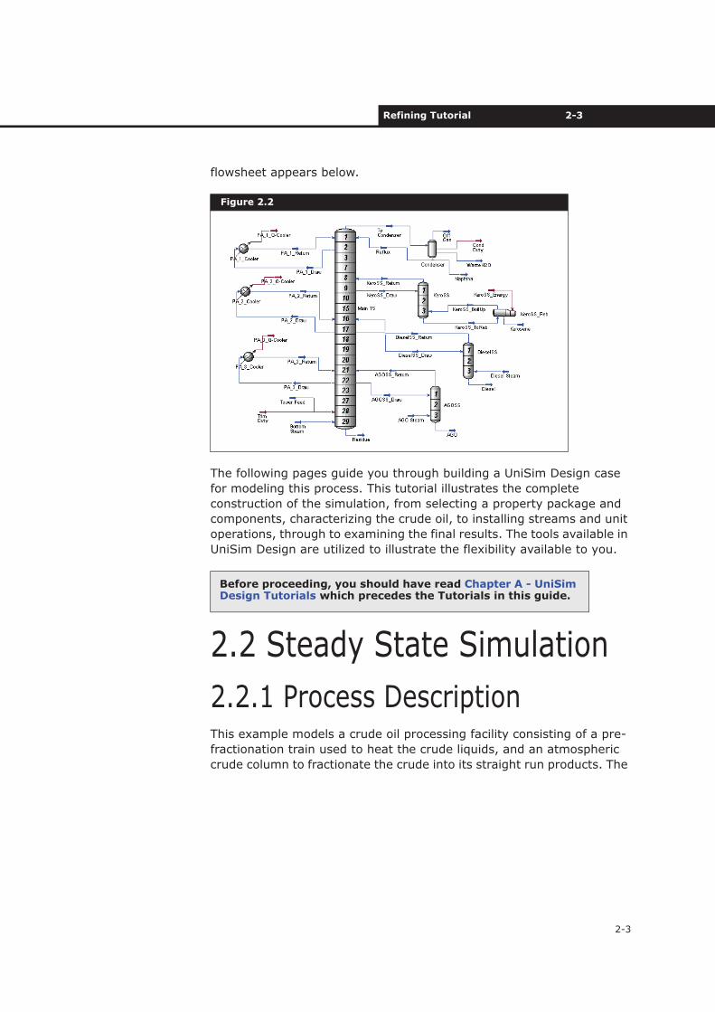
flowsheet appears below.
The following pages guide you through building a UniSim Design case
for modeling this process. This tutorial illustrates the complete
construction of the simulation, from selecting a property package and
components, characterizing the crude oil, to installing streams and unit
operations, through to examining the final results. The tools available in
UniSim Design are utilized to illustrate the flexibility available to you.
2.2 Steady State Simulation
2.2.1 Process DescriptionThis example models a crude oil processing facility consisting of a pre-
fractionation train used to heat the crude liquids, and an atmospheric
crude column to fractionate the crude into its straight run products. The
Figure 2.2
Before proceeding, you should have read Chapter A - UniSim Design Tutorials which precedes the Tutorials in this guide.
2-4 Steady State Simulation
2-4
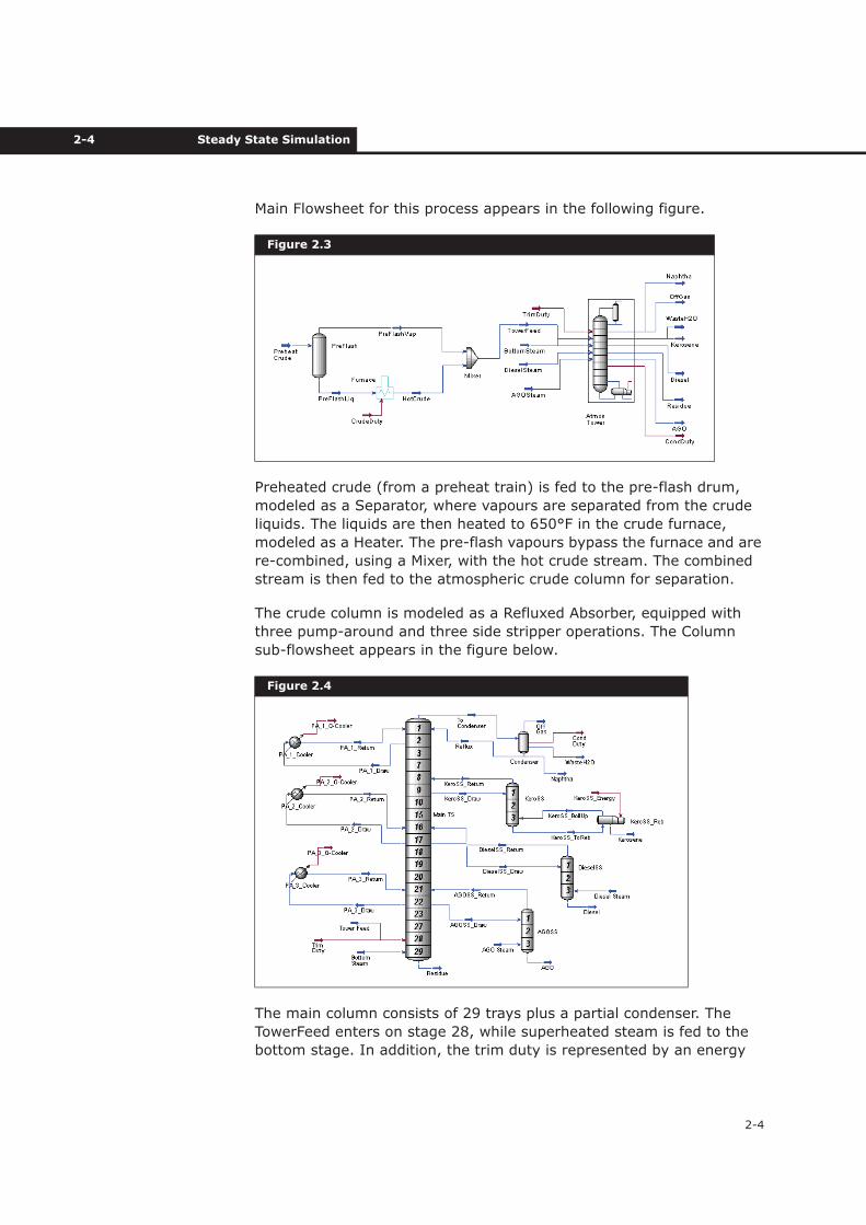
Main Flowsheet for this process appears in the following figure.
Preheated crude (from a preheat train) is fed to the pre-flash drum,
modeled as a Separator, where vapours are separated from the crude
liquids. The liquids are then heated to 650°F in the crude furnace,
modeled as a Heater. The pre-flash vapours bypass the furnace and are
re-combined, using a Mixer, with the hot crude stream. The combined
stream is then fed to the atmospheric crude column for separation.
The crude column is modeled as a Refluxed Absorber, equipped with
three pump-around and three side stripper operations. The Column
sub-flowsheet appears in the figure below.
The main column consists of 29 trays plus a partial condenser. The
TowerFeed enters on stage 28, while superheated steam is fed to the
bottom stage. In addition, the trim duty is represented by an energy
Figure 2.3
Figure 2.4
Refining Tutorial 2-5
2-5
stream feeding onto stage 28. The Naphtha product, as well as the
water stream WasteH2O, are produced from the three-phase
condenser. Crude atmospheric Residue is yielded from the bottom of
the tower.
Each of the three-stage side strippers yields a straight run product.
Kerosene is produced from the reboiled KeroSS side stripper, while
Diesel and AGO (atmospheric gas oil) are produced from the steam-
stripped DieselSS and AGOSS side strippers, respectively.
The two primary building tools, Workbook and PFD, are used to install
the streams and operations and to examine the results while
progressing through the simulation. Both of these tools provide you
with a large amount of flexibility in building your simulation, and in
quickly accessing the information you need.
The Workbook is used to build the first part of the flowsheet, from
specifying the feed conditions through to installing the pre-flash
separator. The PFD is then used to install the remaining operations,
from the crude furnace through to the column.
2.2.2 Setting Your Session Preferences
1. Start UniSim Design and create a new case. The Simulation Basis
The Workbook displays information about streams and unit operations in a tabular format, while the PFD is a graphical representation of the flowsheet.
2-6 Steady State Simulation
2-6
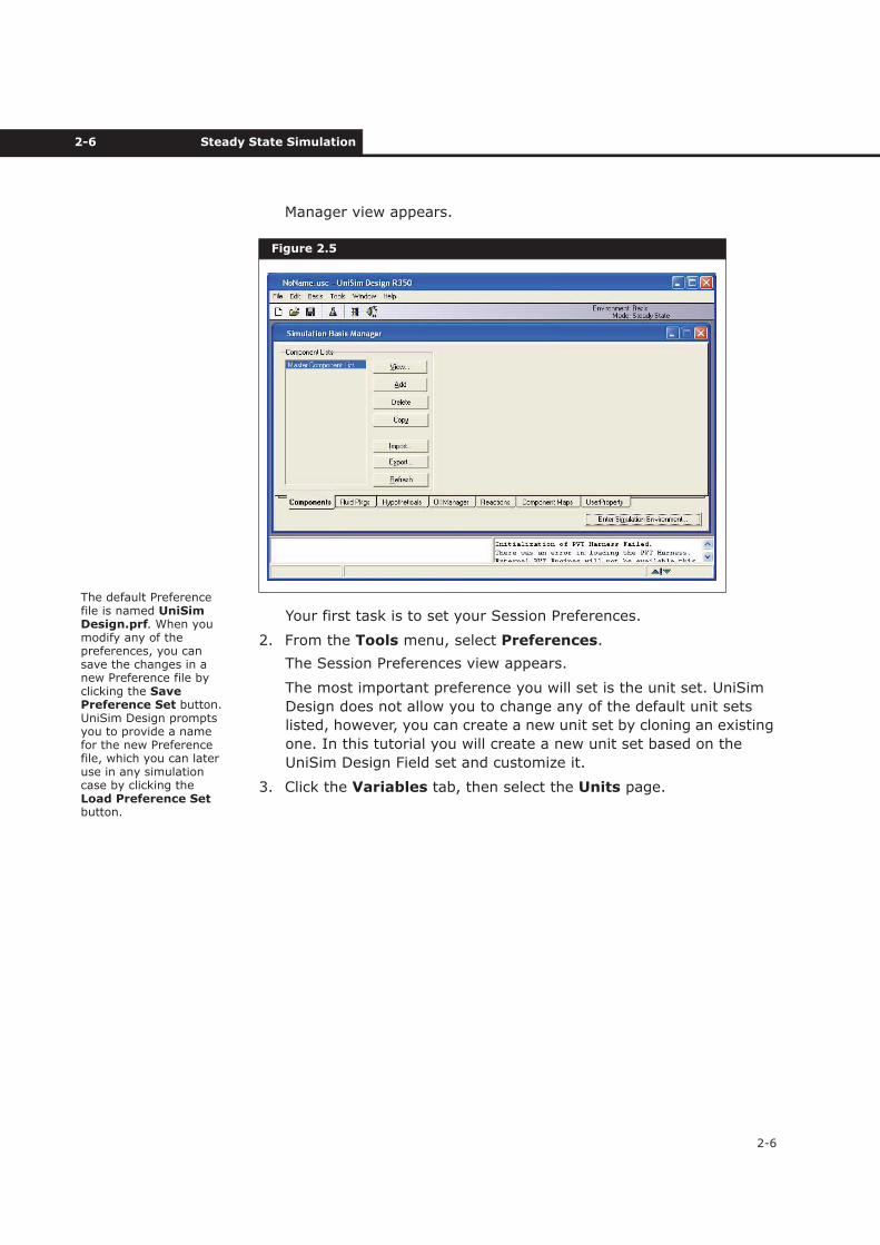
Manager view appears.
Your first task is to set your Session Preferences.
2. From the Tools menu, select Preferences.
The Session Preferences view appears.
The most important preference you will set is the unit set. UniSim
Design does not allow you to change any of the default unit sets
listed, however, you can create a new unit set by cloning an existing
one. In this tutorial you will create a new unit set based on the
UniSim Design Field set and customize it.
3. Click the Variables tab, then select the Units page.
Figure 2.5
The default Preference file is named UniSim Design.prf. When you modify any of the preferences, you can save the changes in a new Preference file by clicking the Save Preference Set button. UniSim Design prompts you to provide a name for the new Preference file, which you can later use in any simulation case by clicking the Load Preference Setbutton.
Refining Tutorial 2-7
2-7
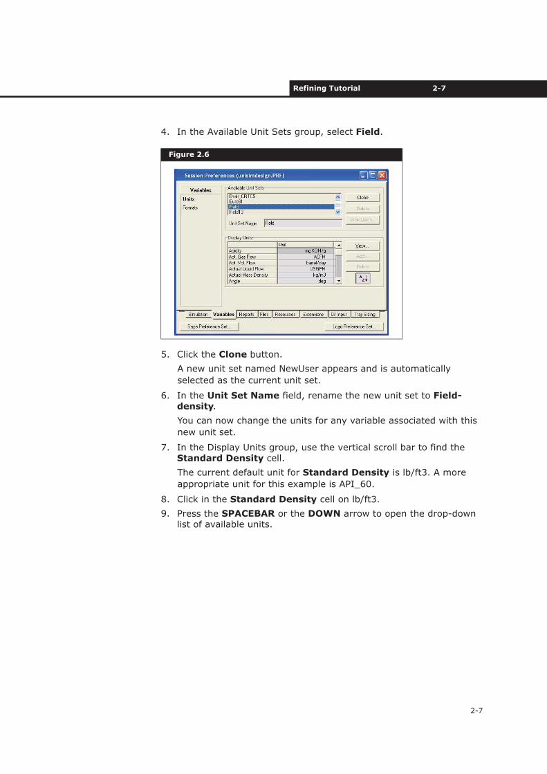
4. In the Available Unit Sets group, select Field.
5. Click the Clone button.
A new unit set named NewUser appears and is automatically
selected as the current unit set.
6. In the Unit Set Name field, rename the new unit set to Field-density.
You can now change the units for any variable associated with this
new unit set.
7. In the Display Units group, use the vertical scroll bar to find the Standard Density cell.
The current default unit for Standard Density is lb/ft3. A more
appropriate unit for this example is API_60.
8. Click in the Standard Density cell on lb/ft3.
9. Press the SPACEBAR or the DOWN arrow to open the drop-down list of available units.
Figure 2.6
2-8 Steady State Simulation
2-8
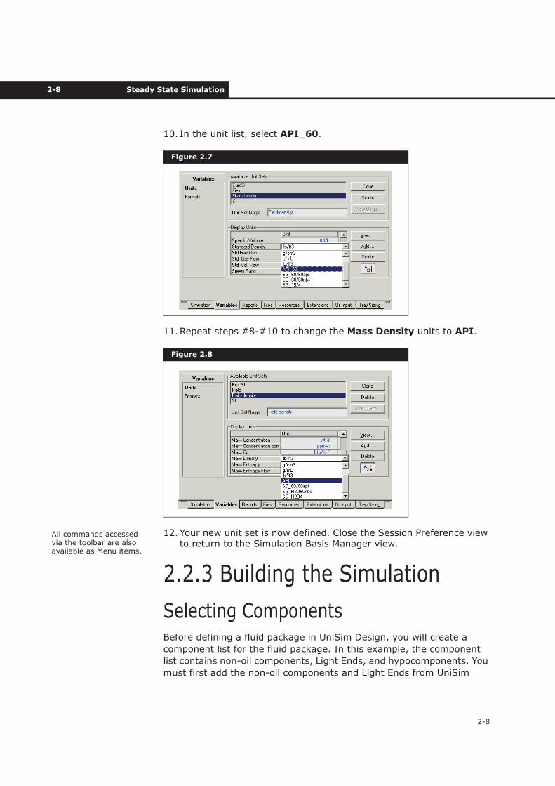
10. In the unit list, select API_60.
11.Repeat steps #8-#10 to change the Mass Density units to API.
12. Your new unit set is now defined. Close the Session Preference view to return to the Simulation Basis Manager view.
2.2.3 Building the Simulation
Selecting ComponentsBefore defining a fluid package in UniSim Design, you will create a
component list for the fluid package. In this example, the component
list contains non-oil components, Light Ends, and hypocomponents. You
must first add the non-oil components and Light Ends from UniSim
Figure 2.7
Figure 2.8
All commands accessed via the toolbar are also available as Menu items.
Refining Tutorial 2-9
2-9
Design pure component library into the component list.
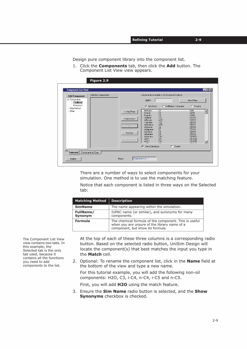
1. Click the Components tab, then click the Add button. The Component List View view appears.
There are a number of ways to select components for your
simulation. One method is to use the matching feature.
Notice that each component is listed in three ways on the Selected
tab:
At the top of each of these three columns is a corresponding radio
button. Based on the selected radio button, UniSim Design will
locate the component(s) that best matches the input you type in
the Match cell.
2. Optional: To rename the component list, click in the Name field at the bottom of the view and type a new name.
For this tutorial example, you will add the following non-oil
components: H2O, C3, i-C4, n-C4, i-C5 and n-C5.
First, you will add H2O using the match feature.
3. Ensure the Sim Name radio button is selected, and the Show Synonyms checkbox is checked.
Figure 2.9
Matching Method Description
SimName The name appearing within the simulation.
FullName/Synonym
IUPAC name (or similar), and synonyms for many components.
Formula The chemical formula of the component. This is useful when you are unsure of the library name of a component, but know its formula.
The Component List View view contains two tabs. In this example, the Selected tab is the only tab used, because it contains all the functions you need to add components to the list.
2-10 Steady State Simulation
2-10
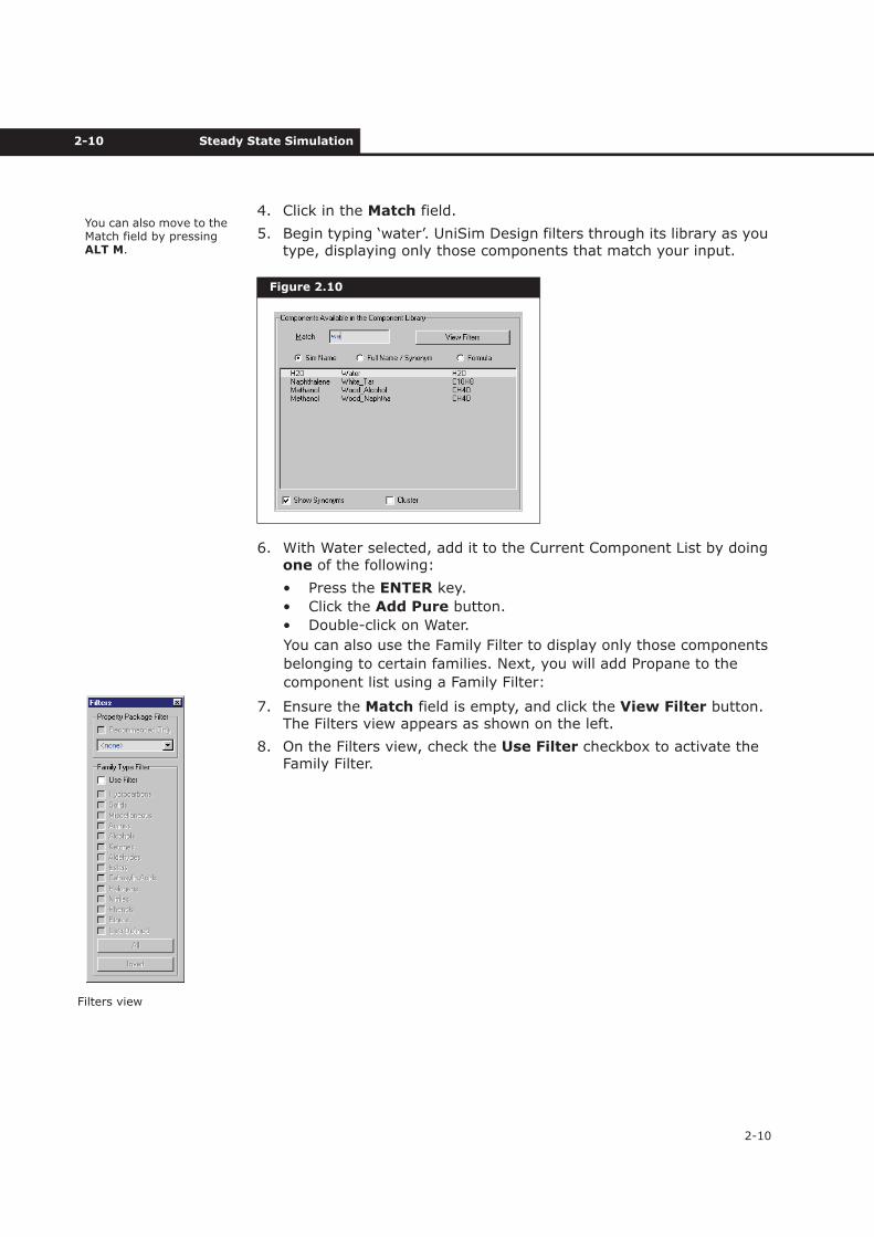
4. Click in the Match field.
5. Begin typing ‘water’. UniSim Design filters through its library as you type, displaying only those components that match your input.
6. With Water selected, add it to the Current Component List by doing one of the following:
• Press the ENTER key.
• Click the Add Pure button.
• Double-click on Water.
You can also use the Family Filter to display only those components
belonging to certain families. Next, you will add Propane to the
component list using a Family Filter:
7. Ensure the Match field is empty, and click the View Filter button. The Filters view appears as shown on the left.
8. On the Filters view, check the Use Filter checkbox to activate the Family Filter.
Figure 2.10
You can also move to the Match field by pressing ALT M.
Filters view
Refining Tutorial 2-11
2-11
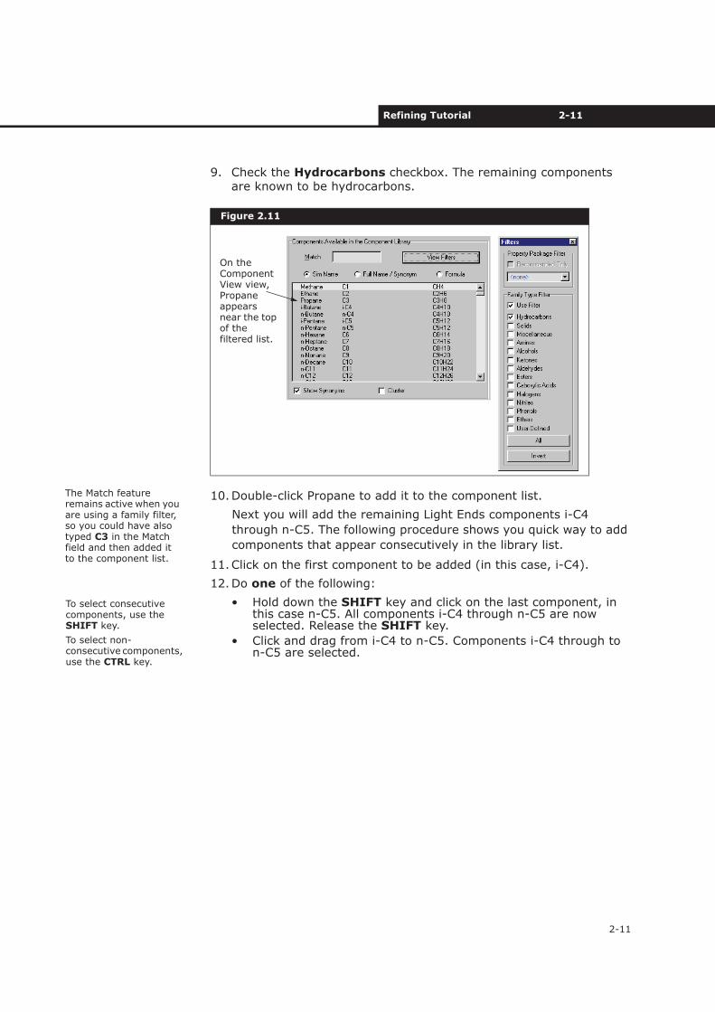
9. Check the Hydrocarbons checkbox. The remaining components are known to be hydrocarbons.
10.Double-click Propane to add it to the component list.
Next you will add the remaining Light Ends components i-C4
through n-C5. The following procedure shows you quick way to add
components that appear consecutively in the library list.
11.Click on the first component to be added (in this case, i-C4).
12.Do one of the following:
• Hold down the SHIFT key and click on the last component, in this case n-C5. All components i-C4 through n-C5 are now selected. Release the SHIFT key.
• Click and drag from i-C4 to n-C5. Components i-C4 through to n-C5 are selected.
Figure 2.11
On the Component View view, Propane appearsnear the top of the filtered list.
The Match feature remains active when you are using a family filter, so you could have also typed C3 in the Match field and then added it to the component list.
To select consecutive components, use the SHIFT key.
To select non-consecutive components, use the CTRL key.
2-12 Steady State Simulation
2-12
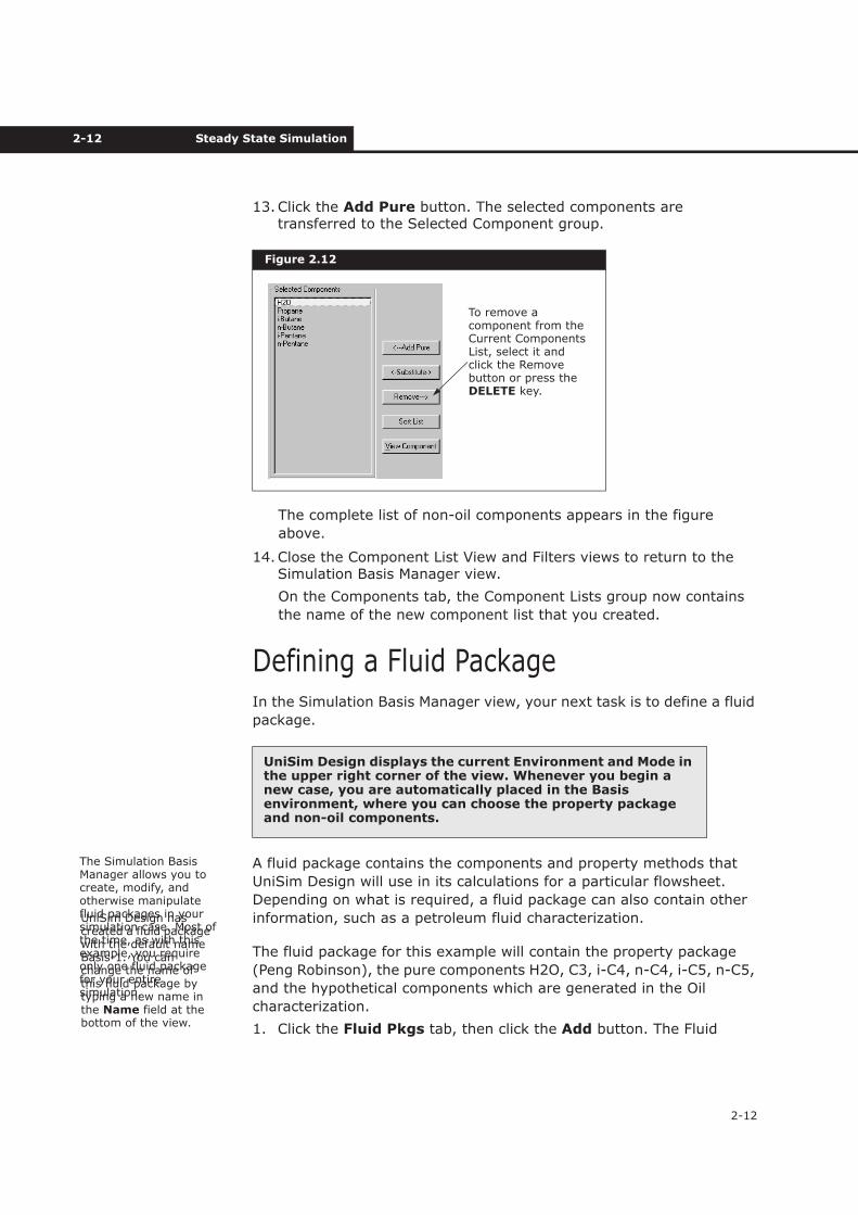
13.Click the Add Pure button. The selected components are transferred to the Selected Component group.
The complete list of non-oil components appears in the figure
above.
14.Close the Component List View and Filters views to return to the Simulation Basis Manager view.
On the Components tab, the Component Lists group now contains
the name of the new component list that you created.
Defining a Fluid PackageIn the Simulation Basis Manager view, your next task is to define a fluid
package.
A fluid package contains the components and property methods that
UniSim Design will use in its calculations for a particular flowsheet.
Depending on what is required, a fluid package can also contain other
information, such as a petroleum fluid characterization.
The fluid package for this example will contain the property package
(Peng Robinson), the pure components H2O, C3, i-C4, n-C4, i-C5, n-C5,
and the hypothetical components which are generated in the Oil
characterization.
1. Click the Fluid Pkgs tab, then click the Add button. The Fluid
Figure 2.12
UniSim Design displays the current Environment and Mode in the upper right corner of the view. Whenever you begin a new case, you are automatically placed in the Basis environment, where you can choose the property package and non-oil components.
To remove a component from the Current Components List, select it and click the Remove button or press the DELETE key.
The Simulation Basis Manager allows you to create, modify, and otherwise manipulate fluid packages in your simulation case. Most of the time, as with this example, you require only one fluid package for your entire simulation.
UniSim Design has created a fluid package with the default name Basis-1. You can change the name of this fluid package by typing a new name in the Name field at the bottom of the view.
Refining Tutorial 2-13
2-13
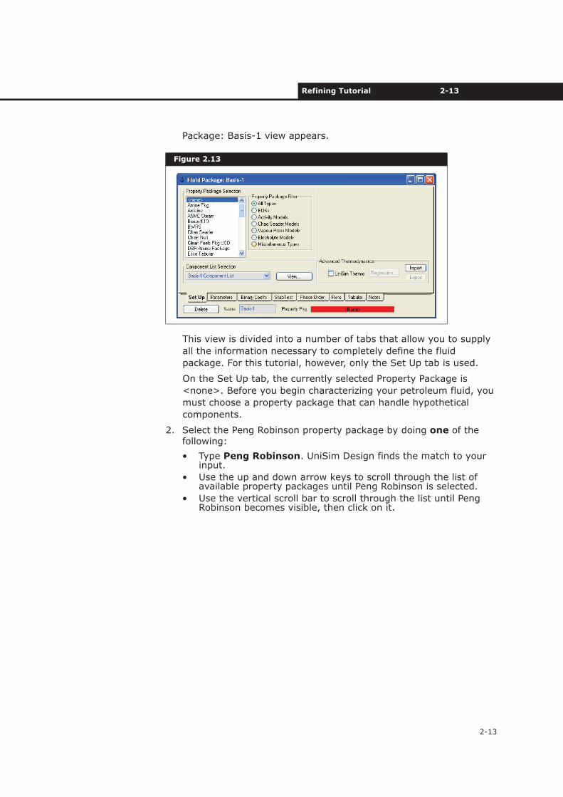
Package: Basis-1 view appears.
This view is divided into a number of tabs that allow you to supply
all the information necessary to completely define the fluid
package. For this tutorial, however, only the Set Up tab is used.
On the Set Up tab, the currently selected Property Package is
<none>. Before you begin characterizing your petroleum fluid, you
must choose a property package that can handle hypothetical
components.
2. Select the Peng Robinson property package by doing one of the following:
• Type Peng Robinson. UniSim Design finds the match to your input.
• Use the up and down arrow keys to scroll through the list of available property packages until Peng Robinson is selected.
• Use the vertical scroll bar to scroll through the list until Peng Robinson becomes visible, then click on it.
Figure 2.13
2-14 Steady State Simulation
2-14
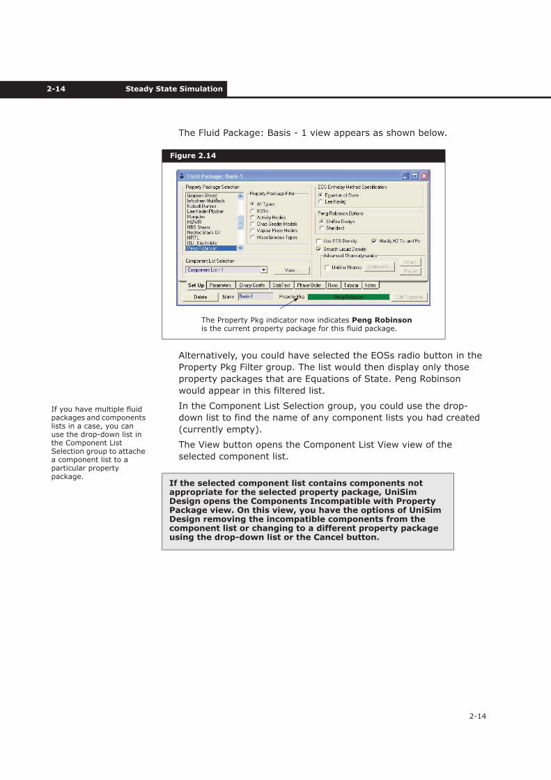
The Fluid Package: Basis - 1 view appears as shown below.
Alternatively, you could have selected the EOSs radio button in the
Property Pkg Filter group. The list would then display only those
property packages that are Equations of State. Peng Robinson
would appear in this filtered list.
In the Component List Selection group, you could use the drop-
down list to find the name of any component lists you had created
(currently empty).
The View button opens the Component List View view of the
selected component list.
Figure 2.14
If the selected component list contains components not appropriate for the selected property package, UniSim Design opens the Components Incompatible with Property Package view. On this view, you have the options of UniSim Design removing the incompatible components from the component list or changing to a different property package using the drop-down list or the Cancel button.
The Property Pkg indicator now indicates Peng Robinsonis the current property package for this fluid package.
If you have multiple fluid packages and components lists in a case, you can use the drop-down list in the Component List Selection group to attache a component list to a particular property package.
Refining Tutorial 2-15
2-15
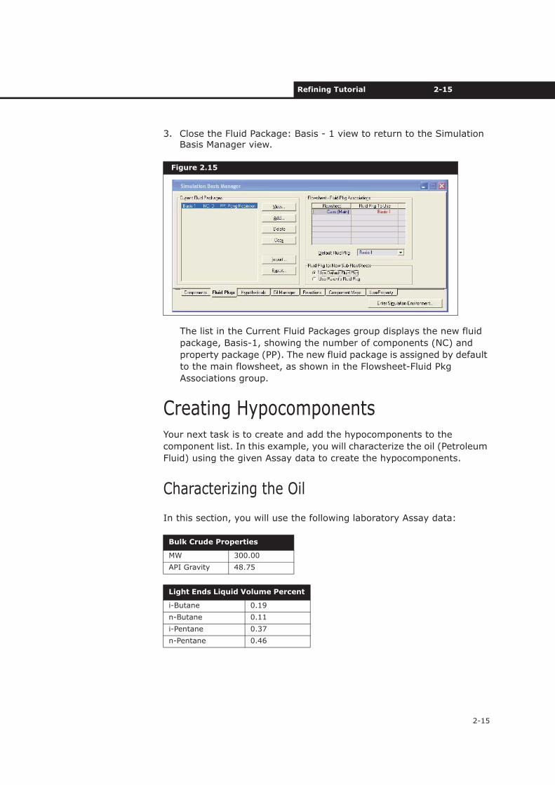
3. Close the Fluid Package: Basis - 1 view to return to the Simulation Basis Manager view.
The list in the Current Fluid Packages group displays the new fluid
package, Basis-1, showing the number of components (NC) and
property package (PP). The new fluid package is assigned by default
to the main flowsheet, as shown in the Flowsheet-Fluid Pkg
Associations group.
Creating HypocomponentsYour next task is to create and add the hypocomponents to the
component list. In this example, you will characterize the oil (Petroleum
Fluid) using the given Assay data to create the hypocomponents.
Characterizing the Oil
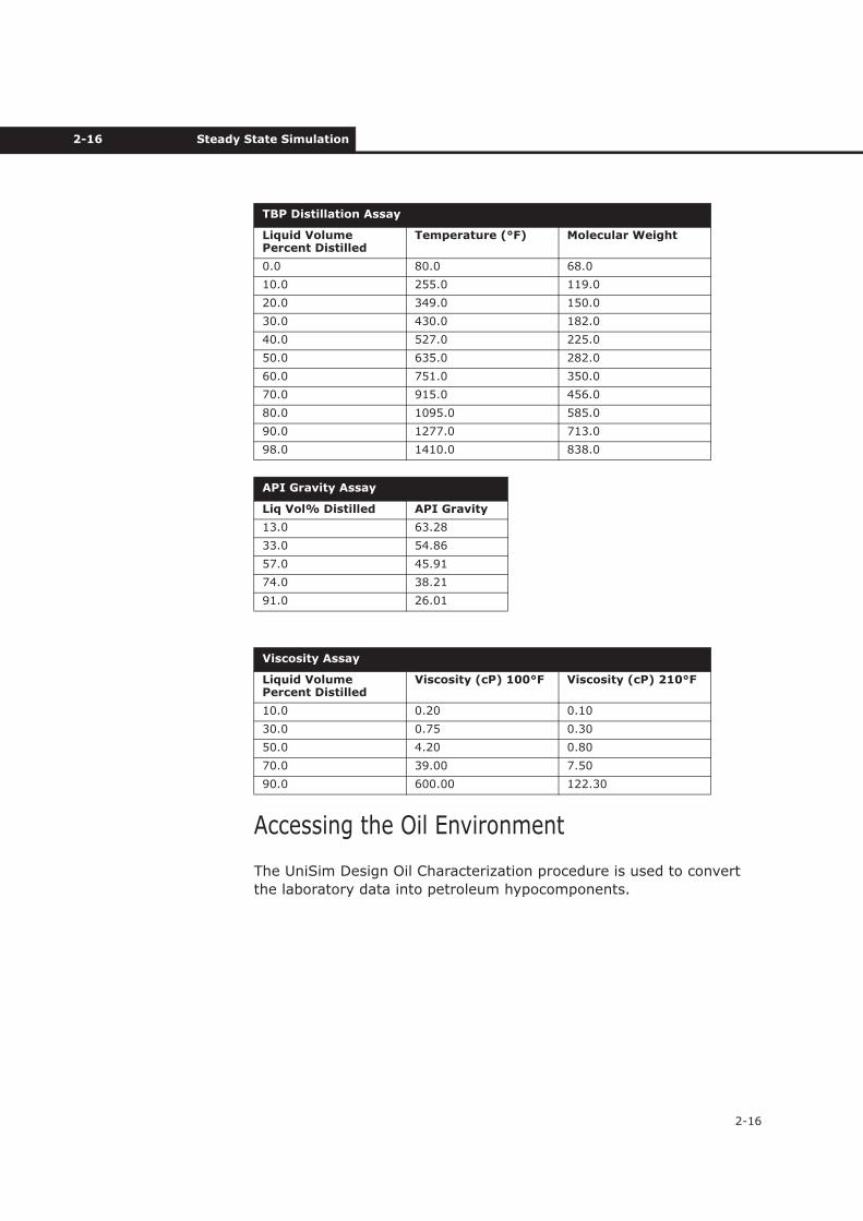
In this section, you will use the following laboratory Assay data:
Figure 2.15
Bulk Crude Properties
MW 300.00
API Gravity 48.75
Light Ends Liquid Volume Percent
i-Butane 0.19
n-Butane 0.11
i-Pentane 0.37
n-Pentane 0.46
2-16 Steady State Simulation
2-16
Accessing the Oil Environment
The UniSim Design Oil Characterization procedure is used to convert
the laboratory data into petroleum hypocomponents.
TBP Distillation Assay
Liquid Volume Percent Distilled
Temperature (°F) Molecular Weight
0.0 80.0 68.0
10.0 255.0 119.0
20.0 349.0 150.0
30.0 430.0 182.0
40.0 527.0 225.0
50.0 635.0 282.0
60.0 751.0 350.0
70.0 915.0 456.0
80.0 1095.0 585.0
90.0 1277.0 713.0
98.0 1410.0 838.0
API Gravity Assay
Liq Vol% Distilled API Gravity
13.0 63.28
33.0 54.86
57.0 45.91
74.0 38.21
91.0 26.01
Viscosity Assay
Liquid Volume Percent Distilled
Viscosity (cP) 100°F Viscosity (cP) 210°F
10.0 0.20 0.10
30.0 0.75 0.30
50.0 4.20 0.80
70.0 39.00 7.50
90.0 600.00 122.30
Refining Tutorial 2-17
2-17
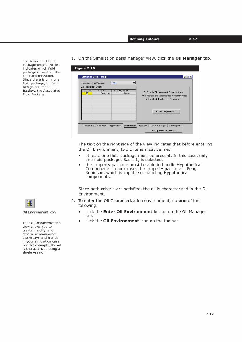
1. On the Simulation Basis Manager view, click the Oil Manager tab.
The text on the right side of the view indicates that before entering
the Oil Environment, two criteria must be met:
• at least one fluid package must be present. In this case, only one fluid package, Basis-1, is selected.
• the property package must be able to handle Hypothetical Components. In our case, the property package is Peng Robinson, which is capable of handling Hypothetical components.
Since both criteria are satisfied, the oil is characterized in the Oil
Environment.
2. To enter the Oil Characterization environment, do one of the following:
• click the Enter Oil Environment button on the Oil Manager tab.
• click the Oil Environment icon on the toolbar.
Figure 2.16
The Associated Fluid Package drop-down list indicates which fluid package is used for the oil characterization. Since there is only one fluid package, UniSim Design has made Basis-1 the Associated Fluid Package.
Oil Environment icon
The Oil Characterization view allows you to create, modify, and otherwise manipulate the Assays and Blends in your simulation case. For this example, the oil is characterized using a single Assay.
2-18 Steady State Simulation
2-18
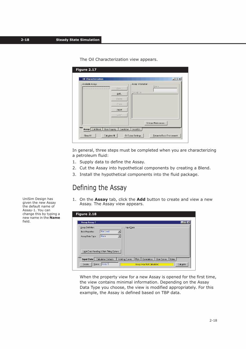
The Oil Characterization view appears.
In general, three steps must be completed when you are characterizing
a petroleum fluid:
1. Supply data to define the Assay.
2. Cut the Assay into hypothetical components by creating a Blend.
3. Install the hypothetical components into the fluid package.
Defining the Assay
1. On the Assay tab, click the Add button to create and view a new Assay. The Assay view appears.
When the property view for a new Assay is opened for the first time,
the view contains minimal information. Depending on the Assay
Data Type you choose, the view is modified appropriately. For this
example, the Assay is defined based on TBP data.
Figure 2.17
Figure 2.18
UniSim Design has given the new Assay the default name of Assay-1. You can change this by typing a new name in the Namefield.
Refining Tutorial 2-19
2-19
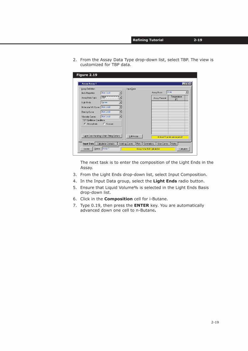
2. From the Assay Data Type drop-down list, select TBP. The view is customized for TBP data.
The next task is to enter the composition of the Light Ends in the
Assay.
3. From the Light Ends drop-down list, select Input Composition.
4. In the Input Data group, select the Light Ends radio button.
5. Ensure that Liquid Volume% is selected in the Light Ends Basis drop-down list.
6. Click in the Composition cell for i-Butane.
7. Type 0.19, then press the ENTER key. You are automatically advanced down one cell to n-Butane.
Figure 2.19
2-20 Steady State Simulation
2-20
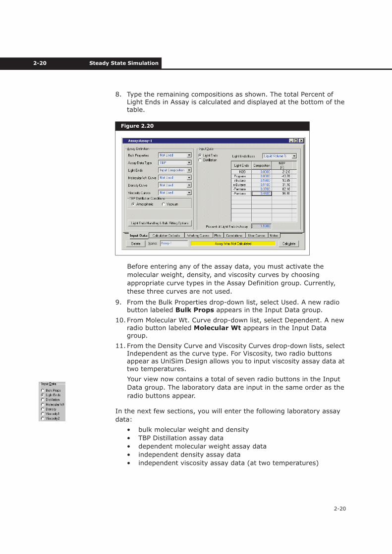
8. Type the remaining compositions as shown. The total Percent of Light Ends in Assay is calculated and displayed at the bottom of the table.
Before entering any of the assay data, you must activate the
molecular weight, density, and viscosity curves by choosing
appropriate curve types in the Assay Definition group. Currently,
these three curves are not used.
9. From the Bulk Properties drop-down list, select Used. A new radio button labeled Bulk Props appears in the Input Data group.
10. From Molecular Wt. Curve drop-down list, select Dependent. A new radio button labeled Molecular Wt appears in the Input Data group.
11. From the Density Curve and Viscosity Curves drop-down lists, select Independent as the curve type. For Viscosity, two radio buttons appear as UniSim Design allows you to input viscosity assay data at two temperatures.
Your view now contains a total of seven radio buttons in the Input
Data group. The laboratory data are input in the same order as the
radio buttons appear.
In the next few sections, you will enter the following laboratory assay
data:
• bulk molecular weight and density
• TBP Distillation assay data
• dependent molecular weight assay data
• independent density assay data
• independent viscosity assay data (at two temperatures)
Figure 2.20
Refining Tutorial 2-21
2-21
Entering Bulk Property Data
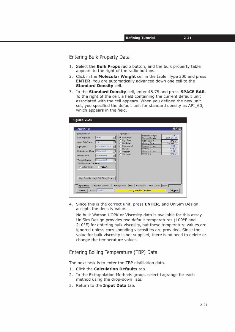
1. Select the Bulk Props radio button, and the bulk property table appears to the right of the radio buttons.
2. Click in the Molecular Weight cell in the table. Type 300 and press ENTER. You are automatically advanced down one cell to the Standard Density cell.
3. In the Standard Density cell, enter 48.75 and press SPACE BAR.To the right of the cell, a field containing the current default unit associated with the cell appears. When you defined the new unit set, you specified the default unit for standard density as API_60, which appears in the field.
4. Since this is the correct unit, press ENTER, and UniSim Design accepts the density value.
No bulk Watson UOPK or Viscosity data is available for this assay.
UniSim Design provides two default temperatures (100°F and
210°F) for entering bulk viscosity, but these temperature values are
ignored unless corresponding viscosities are provided. Since the
value for bulk viscosity is not supplied, there is no need to delete or
change the temperature values.
Entering Boiling Temperature (TBP) Data
The next task is to enter the TBP distillation data.
1. Click the Calculation Defaults tab.
2. In the Extrapolation Methods group, select Lagrange for each method using the drop-down lists.
3. Return to the Input Data tab.
Figure 2.21
2-22 Steady State Simulation
2-22
4. Select the Distillation radio button. The corresponding TBP data matrix appears. UniSim Design displays a message under the matrix, stating that ‘At least 5 points are required’ before the assay can be calculated.
5. From the Assay Basis drop-down list, select Liquid Volume.
6. Click the Edit Assay button. The Assay Input Table view appears.
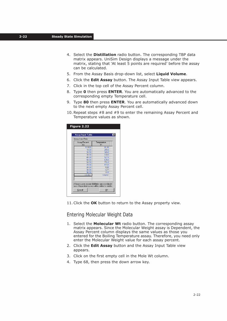
7. Click in the top cell of the Assay Percent column.
8. Type 0 then press ENTER. You are automatically advanced to the corresponding empty Temperature cell.
9. Type 80 then press ENTER. You are automatically advanced down to the next empty Assay Percent cell.
10.Repeat steps #8 and #9 to enter the remaining Assay Percent and Temperature values as shown.
11.Click the OK button to return to the Assay property view.
Entering Molecular Weight Data
1. Select the Molecular Wt radio button. The corresponding assay matrix appears. Since the Molecular Weight assay is Dependent, the Assay Percent column displays the same values as those you entered for the Boiling Temperature assay. Therefore, you need only enter the Molecular Weight value for each assay percent.
2. Click the Edit Assay button and the Assay Input Table view appears.
3. Click on the first empty cell in the Mole Wt column.
4. Type 68, then press the down arrow key.
Figure 2.22
Refining Tutorial 2-23
2-23
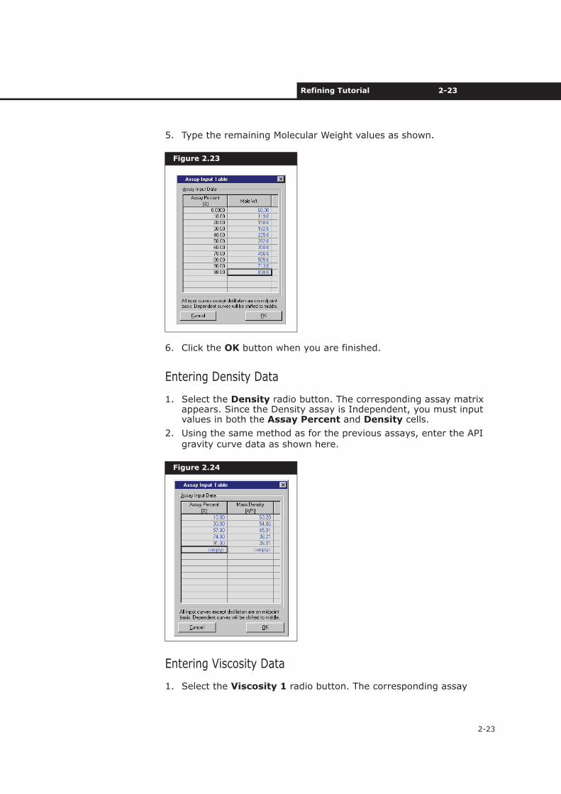
5. Type the remaining Molecular Weight values as shown.
6. Click the OK button when you are finished.
Entering Density Data
1. Select the Density radio button. The corresponding assay matrix appears. Since the Density assay is Independent, you must input values in both the Assay Percent and Density cells.
2. Using the same method as for the previous assays, enter the API gravity curve data as shown here.
Entering Viscosity Data
1. Select the Viscosity 1 radio button. The corresponding assay
Figure 2.23
Figure 2.24
2-24 Steady State Simulation
2-24
matrix appears.
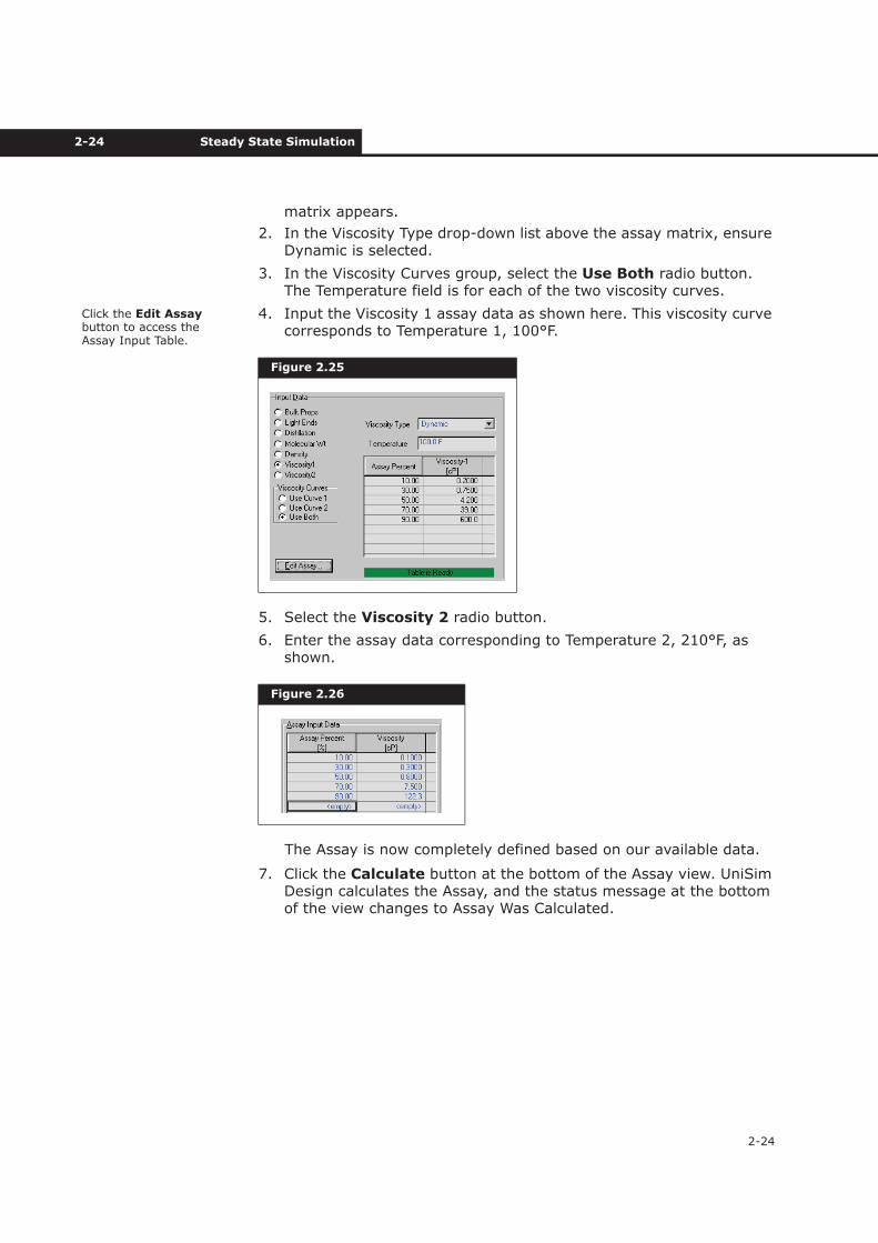
2. In the Viscosity Type drop-down list above the assay matrix, ensure Dynamic is selected.
3. In the Viscosity Curves group, select the Use Both radio button. The Temperature field is for each of the two viscosity curves.
4. Input the Viscosity 1 assay data as shown here. This viscosity curve corresponds to Temperature 1, 100°F.
5. Select the Viscosity 2 radio button.
6. Enter the assay data corresponding to Temperature 2, 210°F, as shown.
The Assay is now completely defined based on our available data.
7. Click the Calculate button at the bottom of the Assay view. UniSim Design calculates the Assay, and the status message at the bottom of the view changes to Assay Was Calculated.
Figure 2.25
Figure 2.26
Click the Edit Assaybutton to access the Assay Input Table.
Refining Tutorial 2-25
2-25
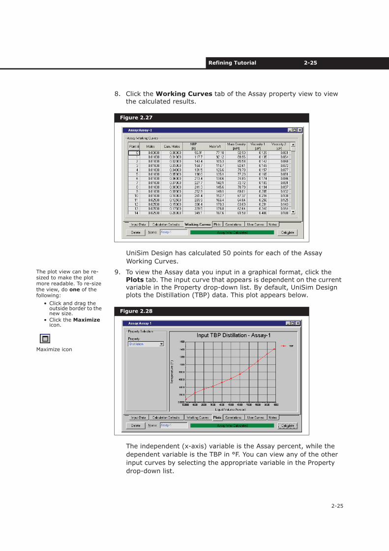
8. Click the Working Curves tab of the Assay property view to view the calculated results.
UniSim Design has calculated 50 points for each of the Assay
Working Curves.
9. To view the Assay data you input in a graphical format, click the Plots tab. The input curve that appears is dependent on the current variable in the Property drop-down list. By default, UniSim Design plots the Distillation (TBP) data. This plot appears below.
The independent (x-axis) variable is the Assay percent, while the
dependent variable is the TBP in °F. You can view any of the other
input curves by selecting the appropriate variable in the Property
drop-down list.
Figure 2.27
Figure 2.28
The plot view can be re-sized to make the plot more readable. To re-size the view, do one of the following:
• Click and drag the outside border to the new size.
• Click the Maximizeicon.
Maximize icon
2-26 Steady State Simulation
2-26
The remaining tabs in the Assay property view provide access to
information which is not required for this tutorial.
10.Close the Assay view to return to the Oil Characterization view.
Cutting the Assay (Creating the Blend)
Now that the assay has been calculated, the next task is to cut the
assay into individual petroleum hypocomponents.
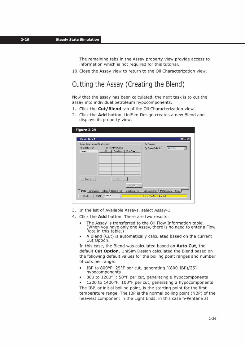
1. Click the Cut/Blend tab of the Oil Characterization view.
2. Click the Add button. UniSim Design creates a new Blend and displays its property view.
3. In the list of Available Assays, select Assay-1.
4. Click the Add button. There are two results:
• The Assay is transferred to the Oil Flow Information table. (When you have only one Assay, there is no need to enter a Flow Rate in this table.)
• A Blend (Cut) is automatically calculated based on the current Cut Option.
In this case, the Blend was calculated based on Auto Cut, the
default Cut Option. UniSim Design calculated the Blend based on
the following default values for the boiling point ranges and number
of cuts per range:
• IBP to 800°F: 25°F per cut, generating [(800-IBP)/25] hypocomponents
• 800 to 1200°F: 50°F per cut, generating 8 hypocomponents
• 1200 to 1400°F: 100°F per cut, generating 2 hypocomponents
The IBP, or initial boiling point, is the starting point for the first
temperature range. The IBP is the normal boiling point (NBP) of the
heaviest component in the Light Ends, in this case n-Pentane at
Figure 2.29
Refining Tutorial 2-27
2-27
96.9°F. The first range results in the generation of (800-96.9)/25 =
28 hypocomponents. All the cut ranges together result in a total of
28+8+2 = 38 hypocomponents.
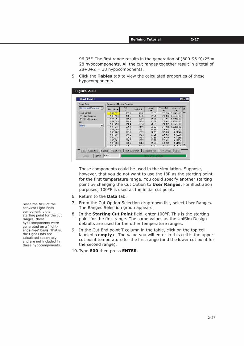
5. Click the Tables tab to view the calculated properties of these hypocomponents.
These components could be used in the simulation. Suppose,
however, that you do not want to use the IBP as the starting point
for the first temperature range. You could specify another starting
point by changing the Cut Option to User Ranges. For illustration
purposes, 100°F is used as the initial cut point.
6. Return to the Data tab.
7. From the Cut Option Selection drop-down list, select User Ranges. The Ranges Selection group appears.
8. In the Starting Cut Point field, enter 100°F. This is the starting point for the first range. The same values as the UniSim Design defaults are used for the other temperature ranges.
9. In the Cut End point T column in the table, click on the top cell labeled <empty>. The value you will enter in this cell is the upper cut point temperature for the first range (and the lower cut point for the second range).
10. Type 800 then press ENTER.
Figure 2.30
Since the NBP of the heaviest Light Ends component is the starting point for the cut ranges, these hypocomponents were generated on a “light-ends-free” basis. That is, the Light Ends are calculated separately and are not included in these hypocomponents.
2-28 Steady State Simulation
2-28
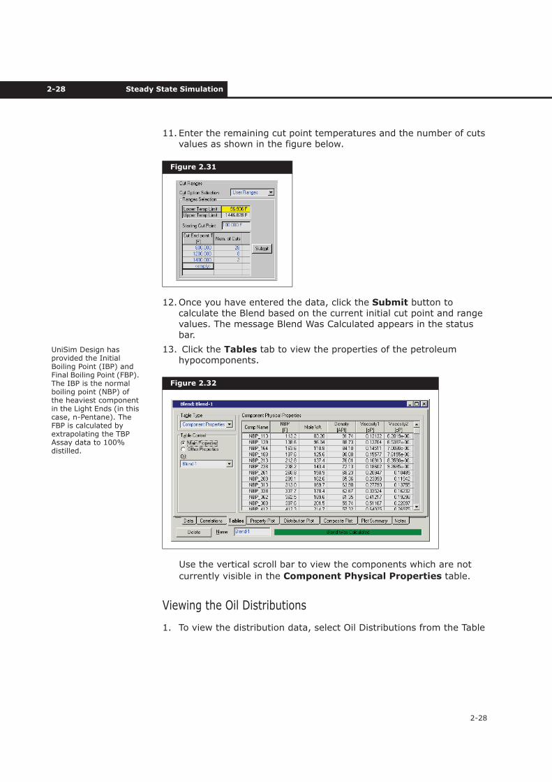
11.Enter the remaining cut point temperatures and the number of cuts values as shown in the figure below.
12.Once you have entered the data, click the Submit button to calculate the Blend based on the current initial cut point and range values. The message Blend Was Calculated appears in the status bar.
13. Click the Tables tab to view the properties of the petroleum hypocomponents.
Use the vertical scroll bar to view the components which are not
currently visible in the Component Physical Properties table.
Viewing the Oil Distributions
1. To view the distribution data, select Oil Distributions from the Table
Figure 2.31
Figure 2.32
UniSim Design has provided the Initial Boiling Point (IBP) and Final Boiling Point (FBP). The IBP is the normal boiling point (NBP) of the heaviest component in the Light Ends (in this case, n-Pentane). The FBP is calculated by extrapolating the TBP Assay data to 100% distilled.
Refining Tutorial 2-29
2-29
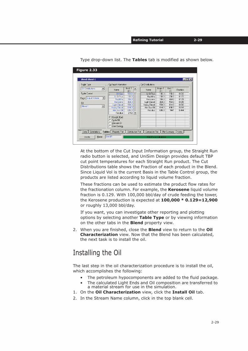
Type drop-down list. The Tables tab is modified as shown below.
At the bottom of the Cut Input Information group, the Straight Run
radio button is selected, and UniSim Design provides default TBP
cut point temperatures for each Straight Run product. The Cut
Distributions table shows the Fraction of each product in the Blend.
Since Liquid Vol is the current Basis in the Table Control group, the
products are listed according to liquid volume fraction.
These fractions can be used to estimate the product flow rates for
the fractionation column. For example, the Kerosene liquid volume
fraction is 0.129. With 100,000 bbl/day of crude feeding the tower,
the Kerosene production is expected at 100,000 * 0.129=12,900
or roughly 13,000 bbl/day.
If you want, you can investigate other reporting and plotting
options by selecting another Table Type or by viewing information
on the other tabs in the Blend property view.
2. When you are finished, close the Blend view to return to the OilCharacterization view. Now that the Blend has been calculated, the next task is to install the oil.
Installing the Oil
The last step in the oil characterization procedure is to install the oil,
which accomplishes the following:
• The petroleum hypocomponents are added to the fluid package.
• The calculated Light Ends and Oil composition are transferred to a material stream for use in the simulation.
1. On the Oil Characterization view, click the Install Oil tab.
2. In the Stream Name column, click in the top blank cell.
Figure 2.33
2-30 Steady State Simulation
2-30
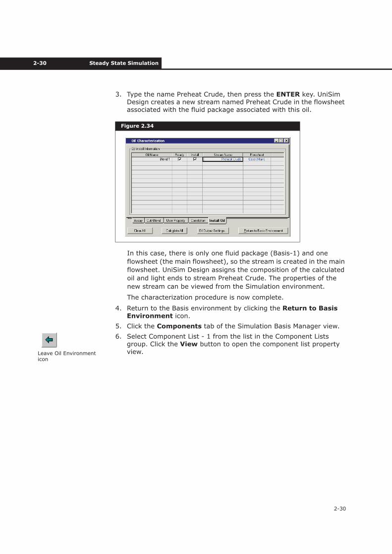
3. Type the name Preheat Crude, then press the ENTER key. UniSim Design creates a new stream named Preheat Crude in the flowsheet associated with the fluid package associated with this oil.
In this case, there is only one fluid package (Basis-1) and one
flowsheet (the main flowsheet), so the stream is created in the main
flowsheet. UniSim Design assigns the composition of the calculated
oil and light ends to stream Preheat Crude. The properties of the
new stream can be viewed from the Simulation environment.
The characterization procedure is now complete.
4. Return to the Basis environment by clicking the Return to Basis Environment icon.
5. Click the Components tab of the Simulation Basis Manager view.
6. Select Component List - 1 from the list in the Component Lists group. Click the View button to open the component list property view.
Figure 2.34
Leave Oil Environment icon
Refining Tutorial 2-31
2-31
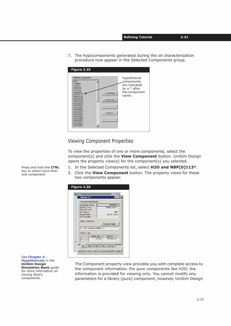
7. The hypocomponents generated during the oil characterization procedure now appear in the Selected Components group.
Viewing Component Properties
To view the properties of one or more components, select the
component(s) and click the View Component button. UniSim Design
opens the property view(s) for the component(s) you selected.
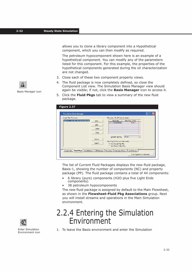
1. In the Selected Components list, select H2O and NBP[0]113*.
2. Click the View Component button. The property views for these two components appear.
The Component property view provides you with complete access to
the component information. For pure components like H2O, the
information is provided for viewing only. You cannot modify any
parameters for a library (pure) component, however, UniSim Design
Figure 2.35
Figure 2.36
Hypothetical components are indicated by a * after the component name.
Press and hold the CTRLkey to select more than one component.
See Chapter 4 - Hypotheticals in the UniSim Design Simulation Basis guide for more information on cloning library components.
2-32 Steady State Simulation
2-32
allows you to clone a library component into a Hypothetical
component, which you can then modify as required.
The petroleum hypocomponent shown here is an example of a
hypothetical component. You can modify any of the parameters
listed for this component. For this example, the properties of the
hypothetical components generated during the oil characterization
are not changed.
3. Close each of these two component property views.
4. The fluid package is now completely defined, so close the Component List view. The Simulation Basis Manager view should again be visible; if not, click the Basis Manager icon to access it.
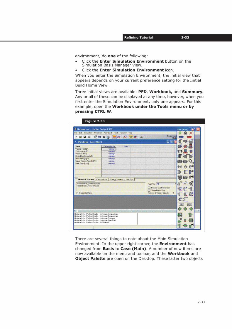
5. Click the Fluid Pkgs tab to view a summary of the new fluid package.
The list of Current Fluid Packages displays the new fluid package,
Basis-1, showing the number of components (NC) and property
package (PP). The fluid package contains a total of 44 components:
• 6 library (pure) components (H2O plus five Light Ends components)
• 38 petroleum hypocomponents
The new fluid package is assigned by default to the Main Flowsheet,
as shown in the Flowsheet-Fluid Pkg Associations group. Next
you will install streams and operations in the Main Simulation
environment.
2.2.4 Entering the Simulation Environment
1. To leave the Basis environment and enter the Simulation
Figure 2.37
Basis Manager icon
Enter Simulation Environment icon
Refining Tutorial 2-33
2-33
environment, do one of the following:
• Click the Enter Simulation Environment button on the Simulation Basis Manager view.
• Click the Enter Simulation Environment icon.
When you enter the Simulation Environment, the initial view that
appears depends on your current preference setting for the Initial
Build Home View.
Three initial views are available: PFD, Workbook, and Summary.
Any or all of these can be displayed at any time, however, when you
first enter the Simulation Environment, only one appears. For this
example, open the Workbook under the Tools menu or by
pressing CTRL W.
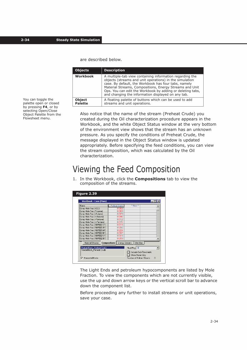
There are several things to note about the Main Simulation
Environment. In the upper right corner, the Environment has
changed from Basis to Case (Main). A number of new items are
now available on the menu and toolbar, and the Workbook and
Object Palette are open on the Desktop. These latter two objects
Figure 2.38
2-34 Steady State Simulation
2-34
are described below.
Also notice that the name of the stream (Preheat Crude) you
created during the Oil characterization procedure appears in the
Workbook, and the white Object Status window at the very bottom
of the environment view shows that the stream has an unknown
pressure. As you specify the conditions of Preheat Crude, the
message displayed in the Object Status window is updated
appropriately. Before specifying the feed conditions, you can view
the stream composition, which was calculated by the Oil
characterization.
Viewing the Feed Composition1. In the Workbook, click the Compositions tab to view the
composition of the streams.
The Light Ends and petroleum hypocomponents are listed by Mole
Fraction. To view the components which are not currently visible,
use the up and down arrow keys or the vertical scroll bar to advance
down the component list.
Before proceeding any further to install streams or unit operations,
save your case.
Objects Description
Workbook A multiple-tab view containing information regarding the objects (streams and unit operations) in the simulation case. By default, the Workbook has four tabs, namely Material Streams, Compositions, Energy Streams and Unit Ops. You can edit the Workbook by adding or deleting tabs, and changing the information displayed on any tab.
Object Palette
A floating palette of buttons which can be used to add streams and unit operations.
Figure 2.39
You can toggle the palette open or closed by pressing F4, or by selecting Open/Close Object Palette from the Flowsheet menu.
Refining Tutorial 2-35
2-35
2. Do one of the following:
• Click the Save icon on the toolbar.
• Select Save from the File menu.
• Press CTRL S.
If this is the first time you have saved your case, the Save
Simulation Case As view appears. By default, the File Path is the
cases sub-directory in your UniSim Design directory.
3. In the File Name field, type a name for the case, for example REFINING. You do not have to enter the *.usc extension; UniSim Design adds it automatically.
4. Once you have entered a file name, press the ENTER key and UniSim Design saves the case under the name you gave it. The Save As view does not appear again unless you choose to give it a new name using the Save As command.
2.2.5 Using the WorkbookClick the Workbook icon on the toolbar to ensure the Workbook view
is active.
Specifying the Feed ConditionsIn general, the first task in the Simulation environment is to install one
or more feed streams, however, the stream Preheat Crude was already
installed during the oil characterization procedure. At this point, your
current location should be the Compositions tab of the Workbook
view.
1. Click the Material Streams tab. The preheated crude enters the pre-fractionation train at 450°F and 75 psia.
2. In the Preheat Crude stream, click in the Temperature cell and type 450. UniSim Design displays the default units for temperature, in this case °F.
3. Since this is the correct unit, press the ENTER key. UniSim Design accepts the temperature. UniSim Design advances to the Pressurecell.
If you know the stream pressure in another unit besides the default
of psia, UniSim Design will accept your input in any one of a number
Figure 2.40
Save icon
If you enter a name that already exists in the current directory, UniSim Design ask you for confirmation before over-writing the existing file.
Workbook icon
When you press ENTERafter entering a stream property, you are advanced down one cell in the Workbook only if the cell below is <empty>. Otherwise, the active cell remains in its current location.
2-36 Steady State Simulation
2-36
of different units and automatically convert the value to the default.
For example, the pressure of Preheat Crude is 5.171 bar, but the
default units are psia.
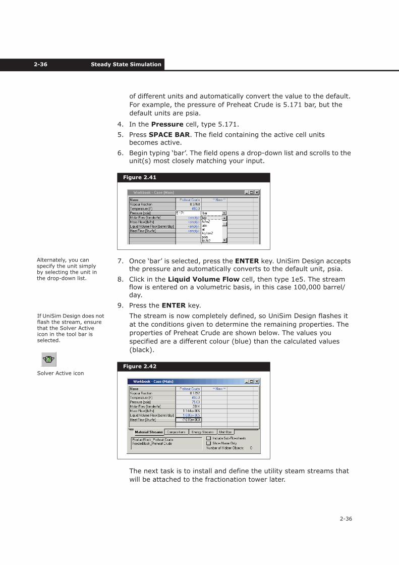
4. In the Pressure cell, type 5.171.
5. Press SPACE BAR. The field containing the active cell units becomes active.
6. Begin typing ‘bar’. The field opens a drop-down list and scrolls to the unit(s) most closely matching your input.
7. Once ‘bar’ is selected, press the ENTER key. UniSim Design accepts the pressure and automatically converts to the default unit, psia.
8. Click in the Liquid Volume Flow cell, then type 1e5. The stream flow is entered on a volumetric basis, in this case 100,000 barrel/day.
9. Press the ENTER key.
The stream is now completely defined, so UniSim Design flashes it
at the conditions given to determine the remaining properties. The
properties of Preheat Crude are shown below. The values you
specified are a different colour (blue) than the calculated values
(black).
The next task is to install and define the utility steam streams that
will be attached to the fractionation tower later.
Figure 2.41
Figure 2.42
Alternately, you can specify the unit simply by selecting the unit in the drop-down list.
If UniSim Design does not flash the stream, ensure that the Solver Active icon in the tool bar is selected.
Solver Active icon
Refining Tutorial 2-37
2-37
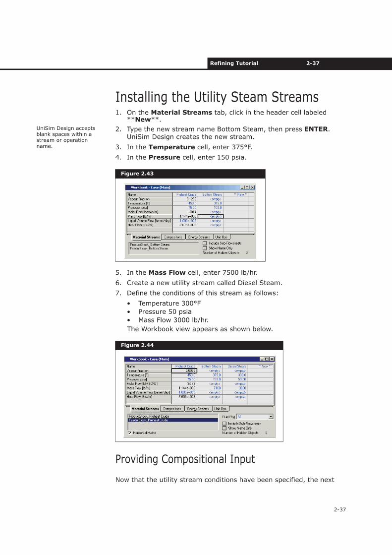
Installing the Utility Steam Streams1. On the Material Streams tab, click in the header cell labeled
**New**.
2. Type the new stream name Bottom Steam, then press ENTER.UniSim Design creates the new stream.
3. In the Temperature cell, enter 375°F.
4. In the Pressure cell, enter 150 psia.
5. In the Mass Flow cell, enter 7500 lb/hr.
6. Create a new utility stream called Diesel Steam.
7. Define the conditions of this stream as follows:
• Temperature 300°F
• Pressure 50 psia
• Mass Flow 3000 lb/hr.
The Workbook view appears as shown below.
Providing Compositional Input
Now that the utility stream conditions have been specified, the next
Figure 2.43
Figure 2.44
UniSim Design accepts blank spaces within a stream or operation name.
2-38 Steady State Simulation
2-38
task is to input the compositions.
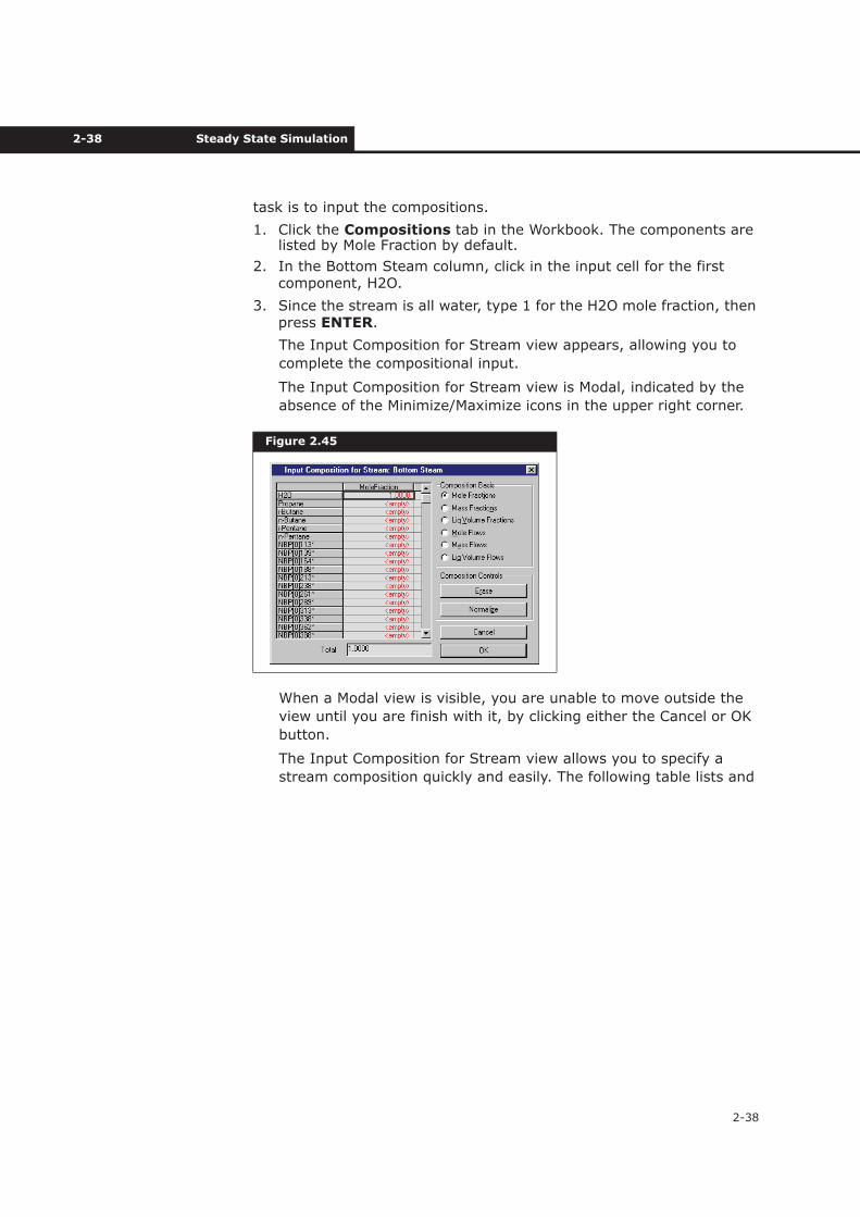
1. Click the Compositions tab in the Workbook. The components are listed by Mole Fraction by default.
2. In the Bottom Steam column, click in the input cell for the first component, H2O.
3. Since the stream is all water, type 1 for the H2O mole fraction, then press ENTER.
The Input Composition for Stream view appears, allowing you to
complete the compositional input.
The Input Composition for Stream view is Modal, indicated by the
absence of the Minimize/Maximize icons in the upper right corner.
When a Modal view is visible, you are unable to move outside the
view until you are finish with it, by clicking either the Cancel or OK
button.
The Input Composition for Stream view allows you to specify a
stream composition quickly and easily. The following table lists and
Figure 2.45
Refining Tutorial 2-39
2-39
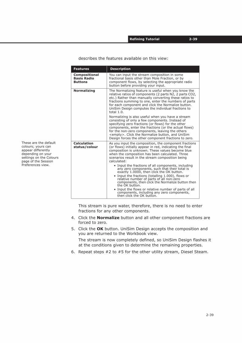
describes the features available on this view:
This stream is pure water, therefore, there is no need to enter
fractions for any other components.
4. Click the Normalize button and all other component fractions are forced to zero.
5. Click the OK button. UniSim Design accepts the composition and you are returned to the Workbook view.
The stream is now completely defined, so UniSim Design flashes it
at the conditions given to determine the remaining properties.
6. Repeat steps #2 to #5 for the other utility stream, Diesel Steam.
Features Description
Compositional Basis Radio Buttons
You can input the stream composition in some fractional basis other than Mole Fraction, or by component flows, by selecting the appropriate radio button before providing your input.
Normalizing The Normalizing feature is useful when you know the relative ratios of components (2 parts N2, 2 parts CO2, etc.) Rather than manually converting these ratios to fractions summing to one, enter the numbers of parts for each component and click the Normalize button. UniSim Design computes the individual fractions to total 1.0.
Normalizing is also useful when you have a stream consisting of only a few components. Instead of specifying zero fractions (or flows) for the other components, enter the fractions (or the actual flows) for the non-zero components, leaving the others <empty>. Click the Normalize button, and UniSim Design forces the other component fractions to zero.
Calculation status/colour
As you input the composition, the component fractions (or flows) initially appear in red, indicating the final composition is unknown. These values become blue when the composition has been calculated. Three scenarios result in the stream composition being calculated:
• Input the fractions of all components, including any zero components, such that their total is exactly 1.0000, then click the OK button.
• Input the fractions (totalling 1.000), flows or relative number of parts of all non-zero components, then click the Normalize button then the OK button.
• Input the flows or relative number of parts of all components, including any zero components, then click the OK button.
These are the default colours; yours can appear differently depending on your settings on the Colours page of the Session Preferences view.
2-40 Steady State Simulation
2-40
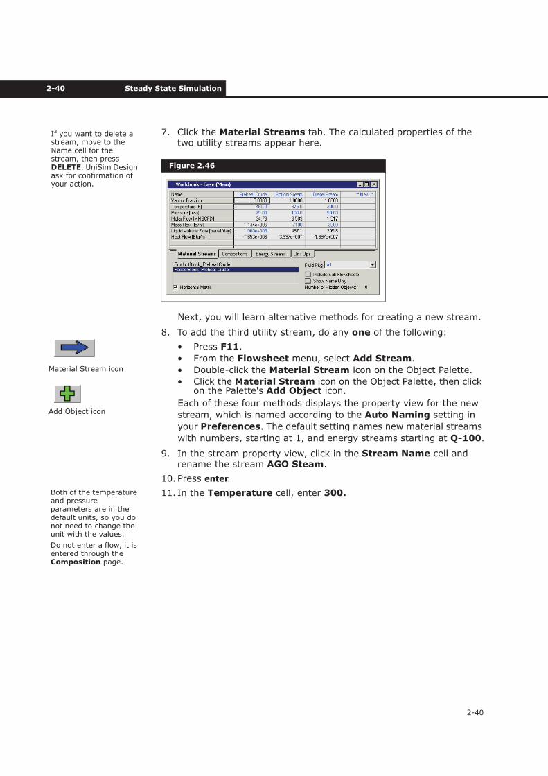
7. Click the Material Streams tab. The calculated properties of the two utility streams appear here.
Next, you will learn alternative methods for creating a new stream.
8. To add the third utility stream, do any one of the following:
• Press F11.
• From the Flowsheet menu, select Add Stream.
• Double-click the Material Stream icon on the Object Palette.
• Click the Material Stream icon on the Object Palette, then click on the Palette's Add Object icon.
Each of these four methods displays the property view for the new
stream, which is named according to the Auto Naming setting in
your Preferences. The default setting names new material streams
with numbers, starting at 1, and energy streams starting at Q-100.
9. In the stream property view, click in the Stream Name cell and rename the stream AGO Steam.
10. Press enter.
11. In the Temperature cell, enter 300.
Figure 2.46
If you want to delete a stream, move to the Name cell for the stream, then press DELETE. UniSim Design ask for confirmation of your action.
Material Stream icon
Add Object icon
Both of the temperature and pressure parameters are in the default units, so you do not need to change the unit with the values.
Do not enter a flow, it is entered through the Composition page.
Refining Tutorial 2-41
2-41
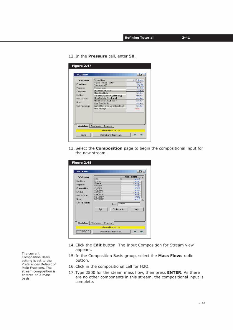
12. In the Pressure cell, enter 50.
13.Select the Composition page to begin the compositional input for the new stream.
14.Click the Edit button. The Input Composition for Stream view appears.
15. In the Composition Basis group, select the Mass Flows radio button.
16.Click in the compositional cell for H2O.
17. Type 2500 for the steam mass flow, then press ENTER. As there are no other components in this stream, the compositional input is complete.
Figure 2.47
Figure 2.48
The current Composition Basis setting is set to the Preferences Default of Mole Fractions. The stream composition is entered on a mass basis.
2-42 Steady State Simulation
2-42
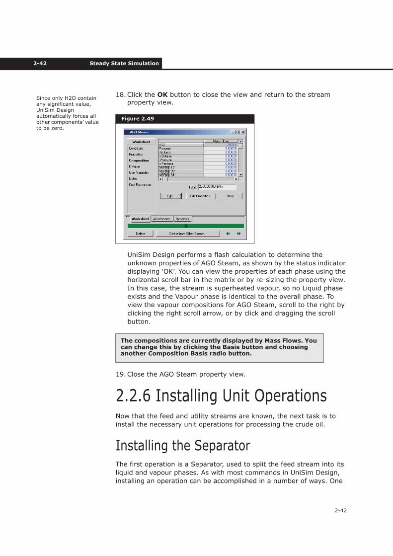
18.Click the OK button to close the view and return to the stream property view.
UniSim Design performs a flash calculation to determine the
unknown properties of AGO Steam, as shown by the status indicator
displaying ‘OK’. You can view the properties of each phase using the
horizontal scroll bar in the matrix or by re-sizing the property view.
In this case, the stream is superheated vapour, so no Liquid phase
exists and the Vapour phase is identical to the overall phase. To
view the vapour compositions for AGO Steam, scroll to the right by
clicking the right scroll arrow, or by click and dragging the scroll
button.
19.Close the AGO Steam property view.
2.2.6 Installing Unit OperationsNow that the feed and utility streams are known, the next task is to
install the necessary unit operations for processing the crude oil.
Installing the SeparatorThe first operation is a Separator, used to split the feed stream into its
liquid and vapour phases. As with most commands in UniSim Design,
installing an operation can be accomplished in a number of ways. One
Figure 2.49
The compositions are currently displayed by Mass Flows. You can change this by clicking the Basis button and choosing another Composition Basis radio button.
Since only H2O contain any significant value, UniSim Design automatically forces all other components’ value to be zero.
Refining Tutorial 2-43
2-43
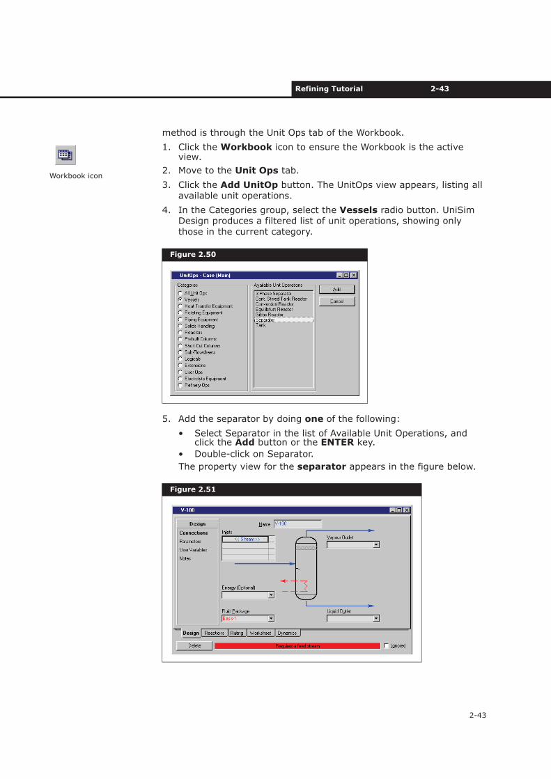
method is through the Unit Ops tab of the Workbook.
1. Click the Workbook icon to ensure the Workbook is the active view.
2. Move to the Unit Ops tab.
3. Click the Add UnitOp button. The UnitOps view appears, listing all available unit operations.
4. In the Categories group, select the Vessels radio button. UniSim Design produces a filtered list of unit operations, showing only those in the current category.
5. Add the separator by doing one of the following:
• Select Separator in the list of Available Unit Operations, and click the Add button or the ENTER key.
• Double-click on Separator.
The property view for the separator appears in the figure below.
Figure 2.50
Figure 2.51
Workbook icon
2-44 Steady State Simulation
2-44
A unit operation property view contains all the information defining
the operation, organized into tabs and pages. The Design, Rating,
and Worksheet tabs appear for most operations. Property views for
more complex operations contain more tabs.
Many operations, like the separator, accept multiple feed streams.
Whenever you see a matrix like the one in the Inlets group, the
operation accepts multiple stream connections at that location.
When the matrix is active, you can access a drop-down list of
available streams.
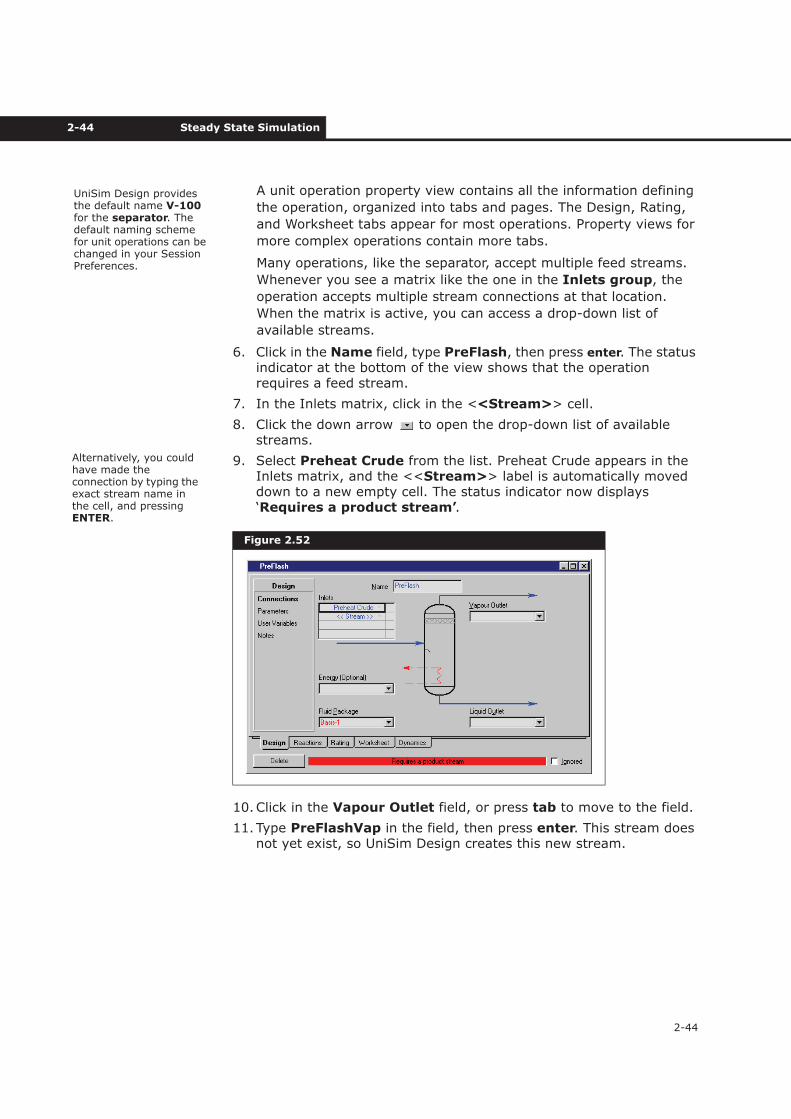
6. Click in the Name field, type PreFlash, then press enter. The status indicator at the bottom of the view shows that the operation requires a feed stream.
7. In the Inlets matrix, click in the <<Stream>> cell.
8. Click the down arrow to open the drop-down list of available streams.
9. Select Preheat Crude from the list. Preheat Crude appears in the Inlets matrix, and the <<Stream>> label is automatically moved down to a new empty cell. The status indicator now displays ‘Requires a product stream’.
10.Click in the Vapour Outlet field, or press tab to move to the field.
11. Type PreFlashVap in the field, then press enter. This stream does not yet exist, so UniSim Design creates this new stream.
Figure 2.52
UniSim Design provides the default name V-100for the separator. The default naming scheme for unit operations can be changed in your Session Preferences.
Alternatively, you could have made the connection by typing the exact stream name in the cell, and pressingENTER.
Refining Tutorial 2-45
2-45
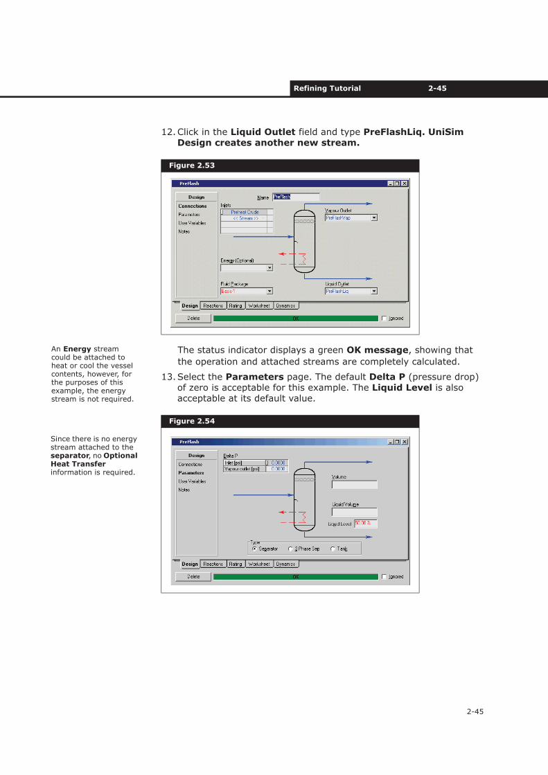
12.Click in the Liquid Outlet field and type PreFlashLiq. UniSim Design creates another new stream.
The status indicator displays a green OK message, showing that
the operation and attached streams are completely calculated.
13.Select the Parameters page. The default Delta P (pressure drop) of zero is acceptable for this example. The Liquid Level is also acceptable at its default value.
Figure 2.53
Figure 2.54
An Energy stream could be attached to heat or cool the vessel contents, however, for the purposes of this example, the energy stream is not required.
Since there is no energy stream attached to the separator, no Optional Heat Transferinformation is required.
2-46 Steady State Simulation
2-46
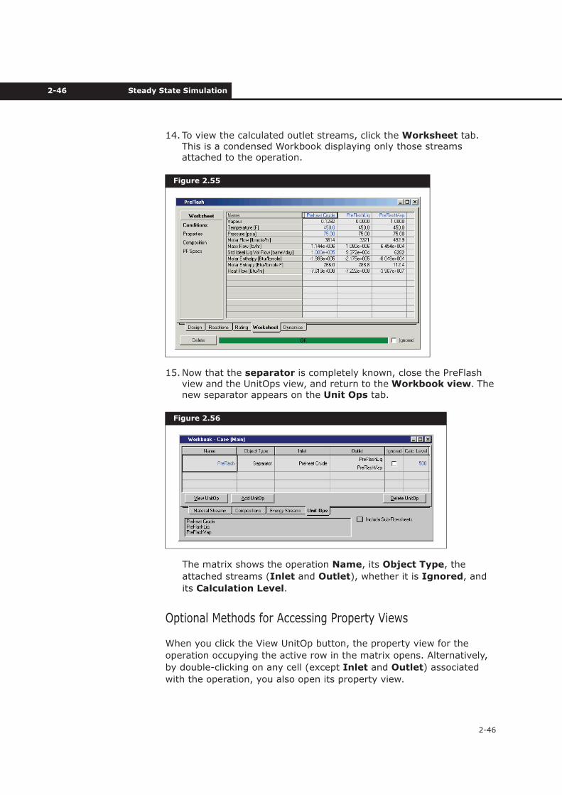
14.To view the calculated outlet streams, click the Worksheet tab. This is a condensed Workbook displaying only those streams attached to the operation.
15.Now that the separator is completely known, close the PreFlash view and the UnitOps view, and return to the Workbook view. The new separator appears on the Unit Ops tab.
The matrix shows the operation Name, its Object Type, the
attached streams (Inlet and Outlet), whether it is Ignored, and
its Calculation Level.
Optional Methods for Accessing Property Views
When you click the View UnitOp button, the property view for the
operation occupying the active row in the matrix opens. Alternatively,
by double-clicking on any cell (except Inlet and Outlet) associated
with the operation, you also open its property view.
Figure 2.55
Figure 2.56
Refining Tutorial 2-47
2-47
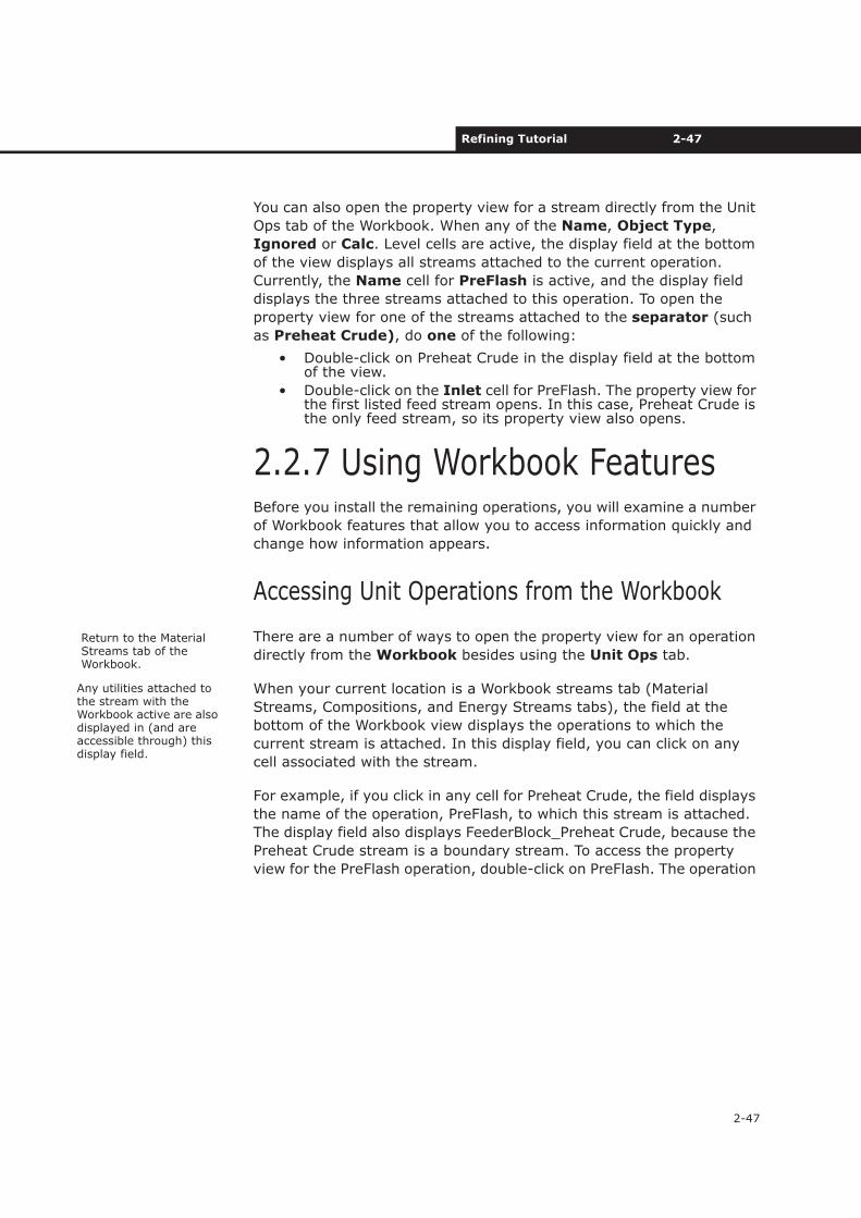
You can also open the property view for a stream directly from the Unit
Ops tab of the Workbook. When any of the Name, Object Type,
Ignored or Calc. Level cells are active, the display field at the bottom
of the view displays all streams attached to the current operation.
Currently, the Name cell for PreFlash is active, and the display field
displays the three streams attached to this operation. To open the
property view for one of the streams attached to the separator (such
as Preheat Crude), do one of the following:
• Double-click on Preheat Crude in the display field at the bottom of the view.
• Double-click on the Inlet cell for PreFlash. The property view for the first listed feed stream opens. In this case, Preheat Crude is the only feed stream, so its property view also opens.
2.2.7 Using Workbook FeaturesBefore you install the remaining operations, you will examine a number
of Workbook features that allow you to access information quickly and
change how information appears.
Accessing Unit Operations from the Workbook
There are a number of ways to open the property view for an operation
directly from the Workbook besides using the Unit Ops tab.
When your current location is a Workbook streams tab (Material
Streams, Compositions, and Energy Streams tabs), the field at the
bottom of the Workbook view displays the operations to which the
current stream is attached. In this display field, you can click on any
cell associated with the stream.
For example, if you click in any cell for Preheat Crude, the field displays
the name of the operation, PreFlash, to which this stream is attached.
The display field also displays FeederBlock_Preheat Crude, because the
Preheat Crude stream is a boundary stream. To access the property
view for the PreFlash operation, double-click on PreFlash. The operation
Return to the Material Streams tab of the Workbook.
Any utilities attached to the stream with the Workbook active are also displayed in (and are accessible through) this display field.
2-48 Steady State Simulation
2-48
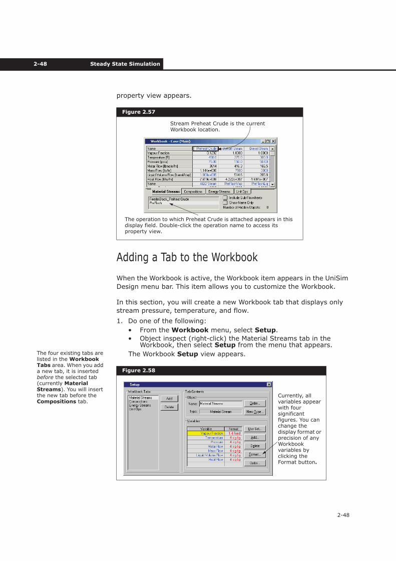
property view appears.
Adding a Tab to the Workbook
When the Workbook is active, the Workbook item appears in the UniSim
Design menu bar. This item allows you to customize the Workbook.
In this section, you will create a new Workbook tab that displays only
stream pressure, temperature, and flow.
1. Do one of the following:
• From the Workbook menu, select Setup.
• Object inspect (right-click) the Material Streams tab in the Workbook, then select Setup from the menu that appears.
The Workbook Setup view appears.
Figure 2.57
Figure 2.58
The operation to which Preheat Crude is attached appears in this display field. Double-click the operation name to access its property view.
Stream Preheat Crude is the current Workbook location.
The four existing tabs are listed in the Workbook Tabs area. When you add a new tab, it is inserted before the selected tab (currently Material Streams). You will insert the new tab before the Compositions tab.
Currently, all variables appear with four significant figures. You can change the display format or precision of any Workbook variables by clicking the Format button.
Refining Tutorial 2-49
2-49
2. In the Workbook Tabs group list, select Compositions.
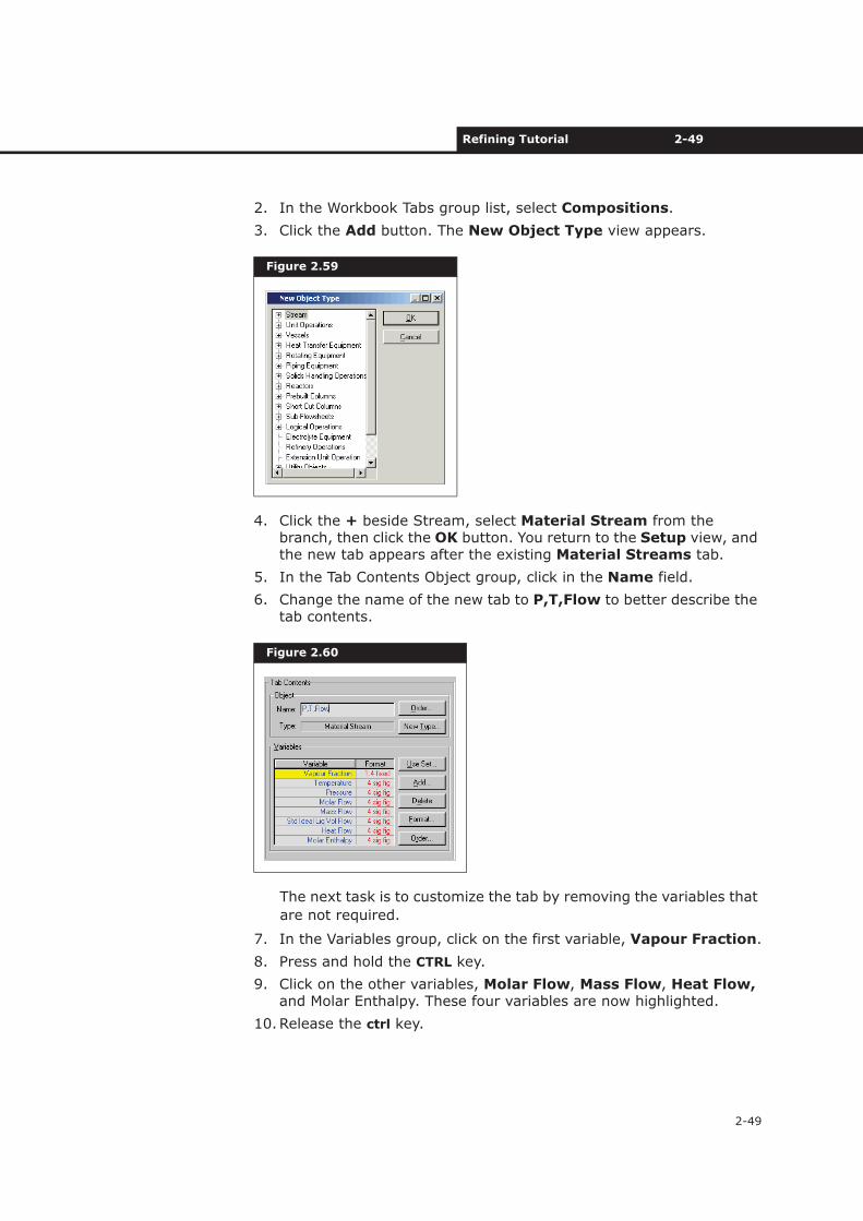
3. Click the Add button. The New Object Type view appears.
4. Click the + beside Stream, select Material Stream from the branch, then click the OK button. You return to the Setup view, and the new tab appears after the existing Material Streams tab.
5. In the Tab Contents Object group, click in the Name field.
6. Change the name of the new tab to P,T,Flow to better describe the tab contents.
The next task is to customize the tab by removing the variables that
are not required.
7. In the Variables group, click on the first variable, Vapour Fraction.
8. Press and hold the CTRL key.
9. Click on the other variables, Molar Flow, Mass Flow, Heat Flow,and Molar Enthalpy. These four variables are now highlighted.
10.Release the ctrl key.
Figure 2.59
Figure 2.60
2-50 Steady State Simulation
2-50
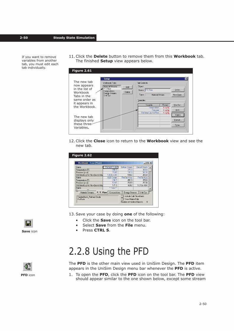
11.Click the Delete button to remove them from this Workbook tab. The finished Setup view appears below.
12.Click the Close icon to return to the Workbook view and see the new tab.
13.Save your case by doing one of the following:
• Click the Save icon on the tool bar.
• Select Save from the File menu.
• Press CTRL S.
2.2.8 Using the PFDThe PFD is the other main view used in UniSim Design. The PFD item
appears in the UniSim Design menu bar whenever the PFD is active.
1. To open the PFD, click the PFD icon on the tool bar. The PFD view should appear similar to the one shown below, except some stream
Figure 2.61
Figure 2.62
If you want to remove variables from another tab, you must edit each tab individually.
The new tab displays only these three Variables.
The new tab now appears in the list of Workbook Tabs in the same order as it appears in the Workbook.
Save icon
PFD icon
Refining Tutorial 2-51
2-51
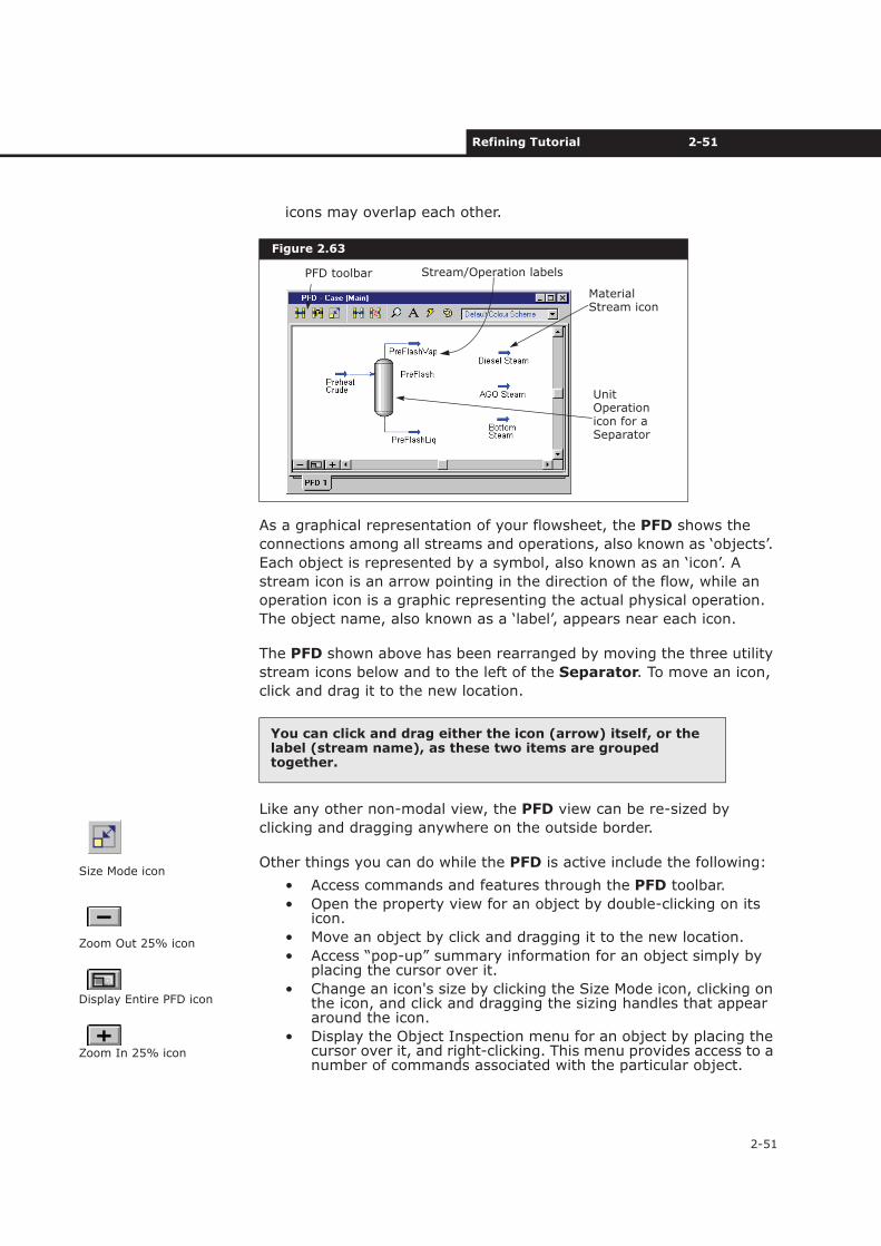
icons may overlap each other.
As a graphical representation of your flowsheet, the PFD shows the
connections among all streams and operations, also known as ‘objects’.
Each object is represented by a symbol, also known as an ‘icon’. A
stream icon is an arrow pointing in the direction of the flow, while an
operation icon is a graphic representing the actual physical operation.
The object name, also known as a ‘label’, appears near each icon.
The PFD shown above has been rearranged by moving the three utility
stream icons below and to the left of the Separator. To move an icon,
click and drag it to the new location.
Like any other non-modal view, the PFD view can be re-sized by
clicking and dragging anywhere on the outside border.
Other things you can do while the PFD is active include the following:
• Access commands and features through the PFD toolbar.
• Open the property view for an object by double-clicking on its icon.
• Move an object by click and dragging it to the new location.
• Access “pop-up” summary information for an object simply by placing the cursor over it.
• Change an icon's size by clicking the Size Mode icon, clicking on the icon, and click and dragging the sizing handles that appear around the icon.
• Display the Object Inspection menu for an object by placing the cursor over it, and right-clicking. This menu provides access to a number of commands associated with the particular object.
Figure 2.63
You can click and drag either the icon (arrow) itself, or the label (stream name), as these two items are grouped together.
PFD toolbar Stream/Operation labels
Unit Operation icon for aSeparator
Material Stream icon
Size Mode icon
Zoom Out 25% icon
Display Entire PFD icon
Zoom In 25% icon
2-52 Steady State Simulation
2-52
• Zoom in and out, or display the entire flowsheet in the PFD window by clicking the zoom buttons at the bottom left corner of the PFD view.
Some of these functions are illustrated here; for more information, see
Section 7.24 - PFD in the UniSim Design User Guide.
Calculation StatusBefore proceeding, you will examine a feature of the PFD that allows
you to trace the calculation status of the objects in your flowsheet. If
you recall, the status indicator at the bottom of the property view for a
stream or operation displays one of three possible states for the object:
When you are in the PFD, the streams and operations are colour-coded
to indicate their calculation status. The inlet separator is completely
calculated, so its normal colours appear. While installing the remaining
operations through the PFD, their colours (and status) changes
appropriately as information is supplied.
A similar colour scheme is used to indicate the status of streams. For
material streams, a dark blue icon indicates the stream has been
flashed and is entirely known. A light blue icon indicates the stream
cannot be flashed until some additional information is supplied.
Similarly, a dark red icon is for an energy stream with a known duty,
while a purple icon indicates an unknown duty.
Installing the Crude Furnace In this section, you will install a crude furnace. The furnace is modeled
as a Heater.
1. Ensure the Object Palette is visible (if it is not, press F4).
You will add the furnace to the right of the PreFlash Separator, so
make some empty space available by scrolling to the right using the
Status Description
Red Status A major piece of defining information is missing from the object. For example, a feed or product stream is not attached to a separator. The status indicator is red, and an appropriate warning message appears.
Yellow Status All major defining information is present, but the stream or operation has not been solved because one or more degrees of freedom is present, for example, a cooler where the outlet stream temperature is unknown. The status indicator is yellow, and an appropriate warning message appears.
Green Status The stream or operation is completely defined and solved. The status indicator is green, and an OK message appears.
Keep in mind that these are the UniSim Design default colours; you can change the colours in the Session Preferences.
The icons for all streams installed to this point are dark blue, indicating they have been flashed.
Heater icon (Red)
Cooler icon (Blue)
Refining Tutorial 2-53
2-53
horizontal scroll bar.
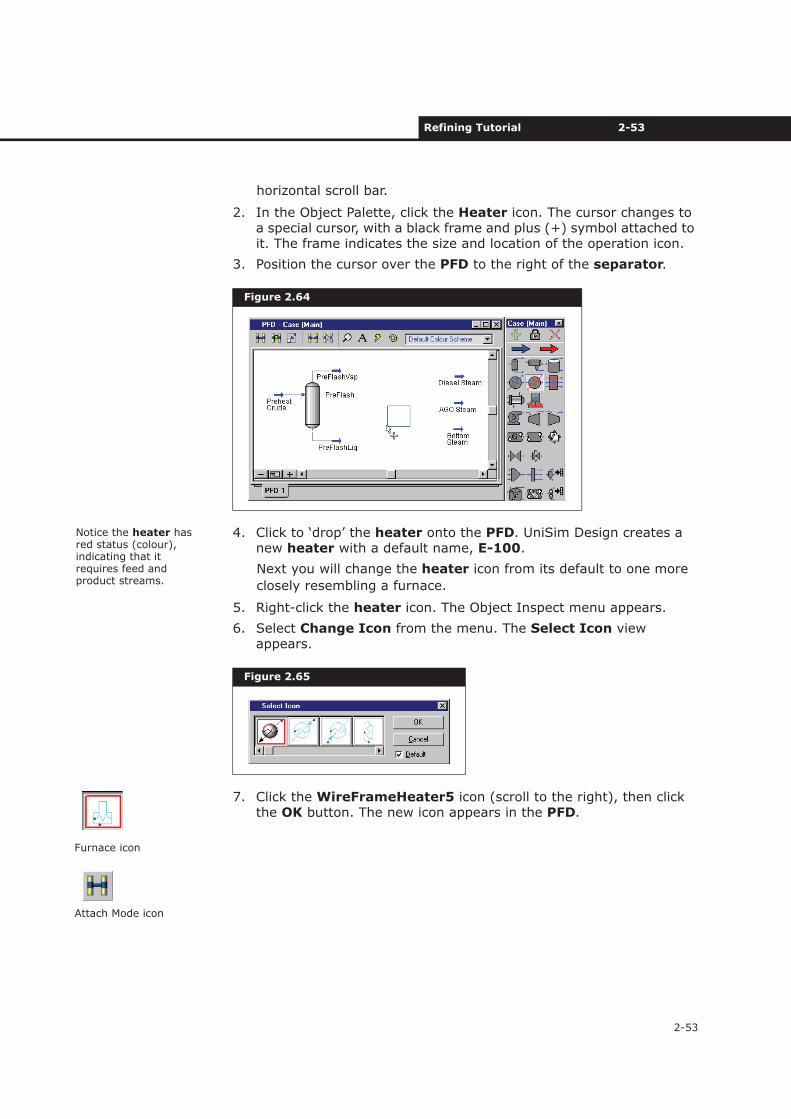
2. In the Object Palette, click the Heater icon. The cursor changes to a special cursor, with a black frame and plus (+) symbol attached to it. The frame indicates the size and location of the operation icon.
3. Position the cursor over the PFD to the right of the separator.
4. Click to ‘drop’ the heater onto the PFD. UniSim Design creates a new heater with a default name, E-100.
Next you will change the heater icon from its default to one more
closely resembling a furnace.
5. Right-click the heater icon. The Object Inspect menu appears.
6. Select Change Icon from the menu. The Select Icon view appears.
7. Click the WireFrameHeater5 icon (scroll to the right), then click the OK button. The new icon appears in the PFD.
Figure 2.64
Figure 2.65
Notice the heater has red status (colour), indicating that it requires feed and product streams.
Furnace icon
Attach Mode icon
2-54 Steady State Simulation
2-54
Attaching Streams to the Furnace
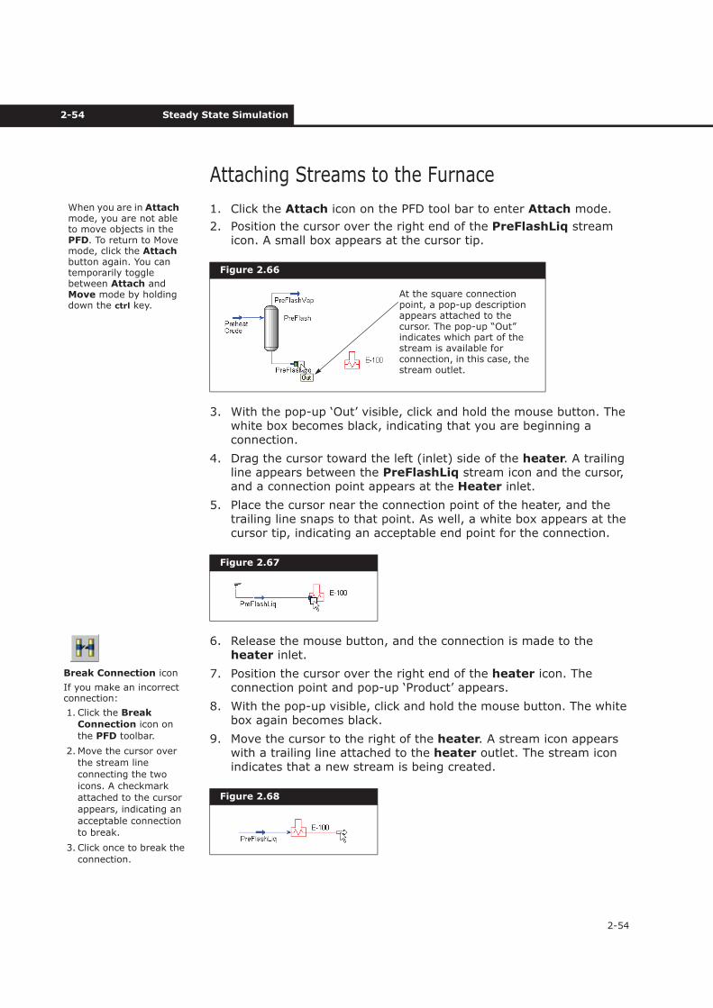
1. Click the Attach icon on the PFD tool bar to enter Attach mode.
2. Position the cursor over the right end of the PreFlashLiq stream icon. A small box appears at the cursor tip.
3. With the pop-up ‘Out’ visible, click and hold the mouse button. The white box becomes black, indicating that you are beginning a connection.
4. Drag the cursor toward the left (inlet) side of the heater. A trailing line appears between the PreFlashLiq stream icon and the cursor, and a connection point appears at the Heater inlet.
5. Place the cursor near the connection point of the heater, and the trailing line snaps to that point. As well, a white box appears at the cursor tip, indicating an acceptable end point for the connection.
6. Release the mouse button, and the connection is made to the heater inlet.
7. Position the cursor over the right end of the heater icon. The connection point and pop-up ‘Product’ appears.
8. With the pop-up visible, click and hold the mouse button. The white box again becomes black.
9. Move the cursor to the right of the heater. A stream icon appears with a trailing line attached to the heater outlet. The stream icon indicates that a new stream is being created.
Figure 2.66
Figure 2.67
Figure 2.68
When you are in Attachmode, you are not able to move objects in the PFD. To return to Move mode, click the Attachbutton again. You can temporarily toggle between Attach and Move mode by holding down the ctrl key.
At the square connection point, a pop-up description appears attached to the cursor. The pop-up “Out” indicates which part of the stream is available for connection, in this case, the stream outlet.
Break Connection icon
If you make an incorrect connection:
1. Click the Break
Connection icon on
the PFD toolbar.
2. Move the cursor over
the stream line
connecting the two
icons. A checkmark
attached to the cursor
appears, indicating an
acceptable connection
to break.
3. Click once to break the
connection.
Refining Tutorial 2-55
2-55
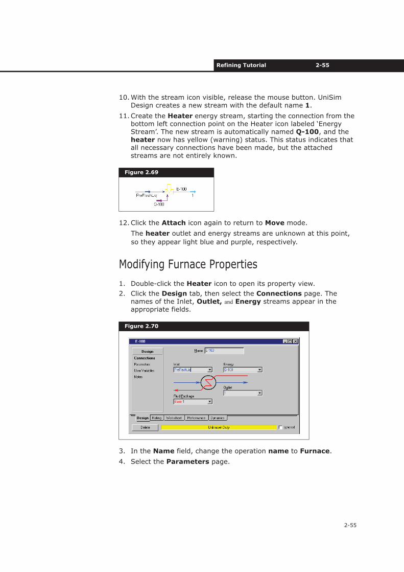
10.With the stream icon visible, release the mouse button. UniSim Design creates a new stream with the default name 1.
11.Create the Heater energy stream, starting the connection from the bottom left connection point on the Heater icon labeled ‘Energy Stream’. The new stream is automatically named Q-100, and the heater now has yellow (warning) status. This status indicates that all necessary connections have been made, but the attached streams are not entirely known.
12.Click the Attach icon again to return to Move mode.
The heater outlet and energy streams are unknown at this point,
so they appear light blue and purple, respectively.
Modifying Furnace Properties
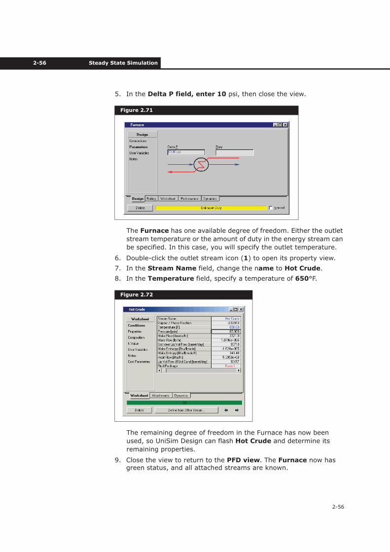
1. Double-click the Heater icon to open its property view.
2. Click the Design tab, then select the Connections page. The names of the Inlet, Outlet, and Energy streams appear in the appropriate fields.
3. In the Name field, change the operation name to Furnace.
4. Select the Parameters page.
Figure 2.69
Figure 2.70
2-56 Steady State Simulation
2-56
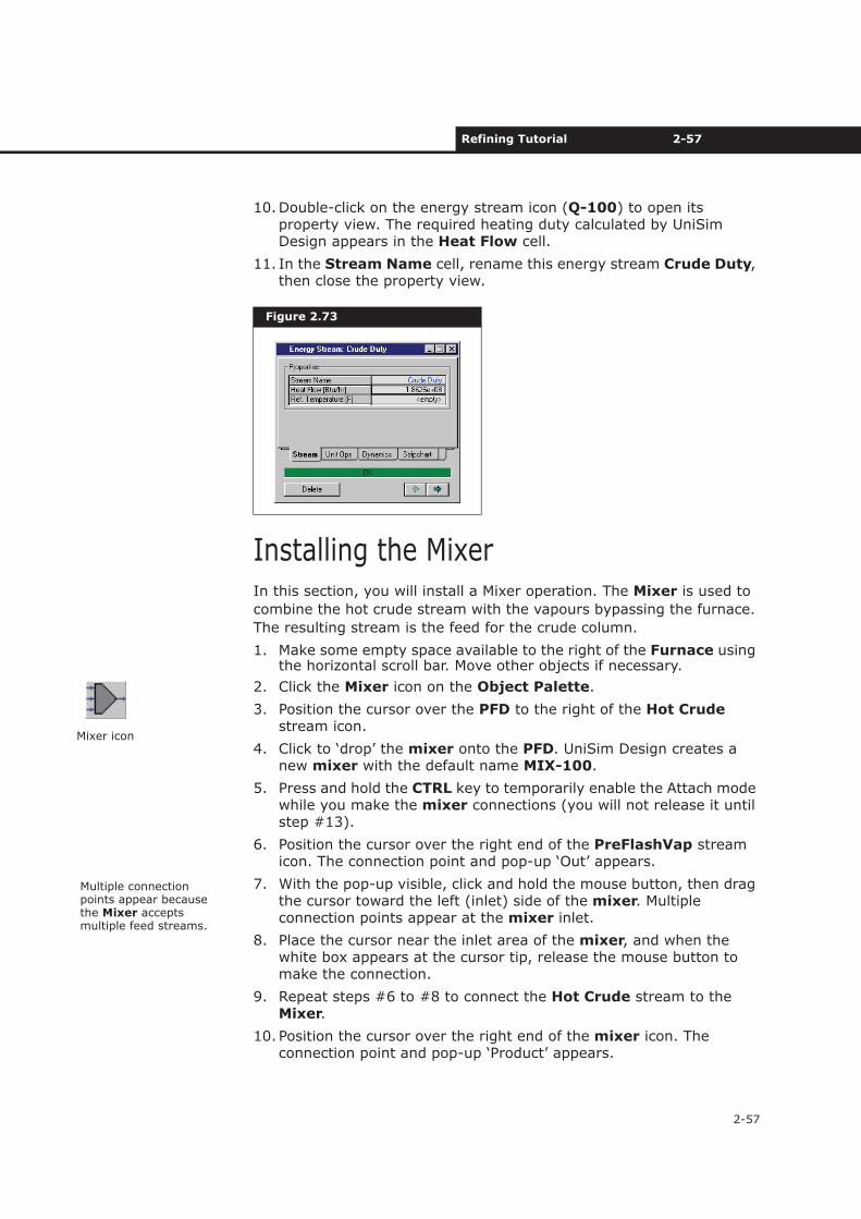
5. In the Delta P field, enter 10 psi, then close the view.
The Furnace has one available degree of freedom. Either the outlet
stream temperature or the amount of duty in the energy stream can
be specified. In this case, you will specify the outlet temperature.
6. Double-click the outlet stream icon (1) to open its property view.
7. In the Stream Name field, change the name to Hot Crude.
8. In the Temperature field, specify a temperature of 650°F.
The remaining degree of freedom in the Furnace has now been
used, so UniSim Design can flash Hot Crude and determine its
remaining properties.
9. Close the view to return to the PFD view. The Furnace now has green status, and all attached streams are known.
Figure 2.71
Figure 2.72
Refining Tutorial 2-57
2-57
10.Double-click on the energy stream icon (Q-100) to open its property view. The required heating duty calculated by UniSim Design appears in the Heat Flow cell.
11. In the Stream Name cell, rename this energy stream Crude Duty,then close the property view.
Installing the Mixer In this section, you will install a Mixer operation. The Mixer is used to
combine the hot crude stream with the vapours bypassing the furnace.
The resulting stream is the feed for the crude column.
1. Make some empty space available to the right of the Furnace using the horizontal scroll bar. Move other objects if necessary.
2. Click the Mixer icon on the Object Palette.
3. Position the cursor over the PFD to the right of the Hot Crudestream icon.
4. Click to ‘drop’ the mixer onto the PFD. UniSim Design creates a new mixer with the default name MIX-100.
5. Press and hold the CTRL key to temporarily enable the Attach mode while you make the mixer connections (you will not release it until step #13).
6. Position the cursor over the right end of the PreFlashVap stream icon. The connection point and pop-up ‘Out’ appears.
7. With the pop-up visible, click and hold the mouse button, then drag the cursor toward the left (inlet) side of the mixer. Multiple connection points appear at the mixer inlet.
8. Place the cursor near the inlet area of the mixer, and when the white box appears at the cursor tip, release the mouse button to make the connection.
9. Repeat steps #6 to #8 to connect the Hot Crude stream to the Mixer.
10. Position the cursor over the right end of the mixer icon. The connection point and pop-up ‘Product’ appears.
Figure 2.73
Mixer icon
Multiple connection points appear because the Mixer accepts multiple feed streams.
2-58 Steady State Simulation
2-58
11.With the pop-up visible, click and drag to the right of the mixer. A white stream icon appears, with a trailing line attached to the mixeroutlet.
12.With the white stream icon visible, release the mouse button. UniSim Design creates a new stream with the default name 1.
13.Release the ctrl key to leave Attach mode.
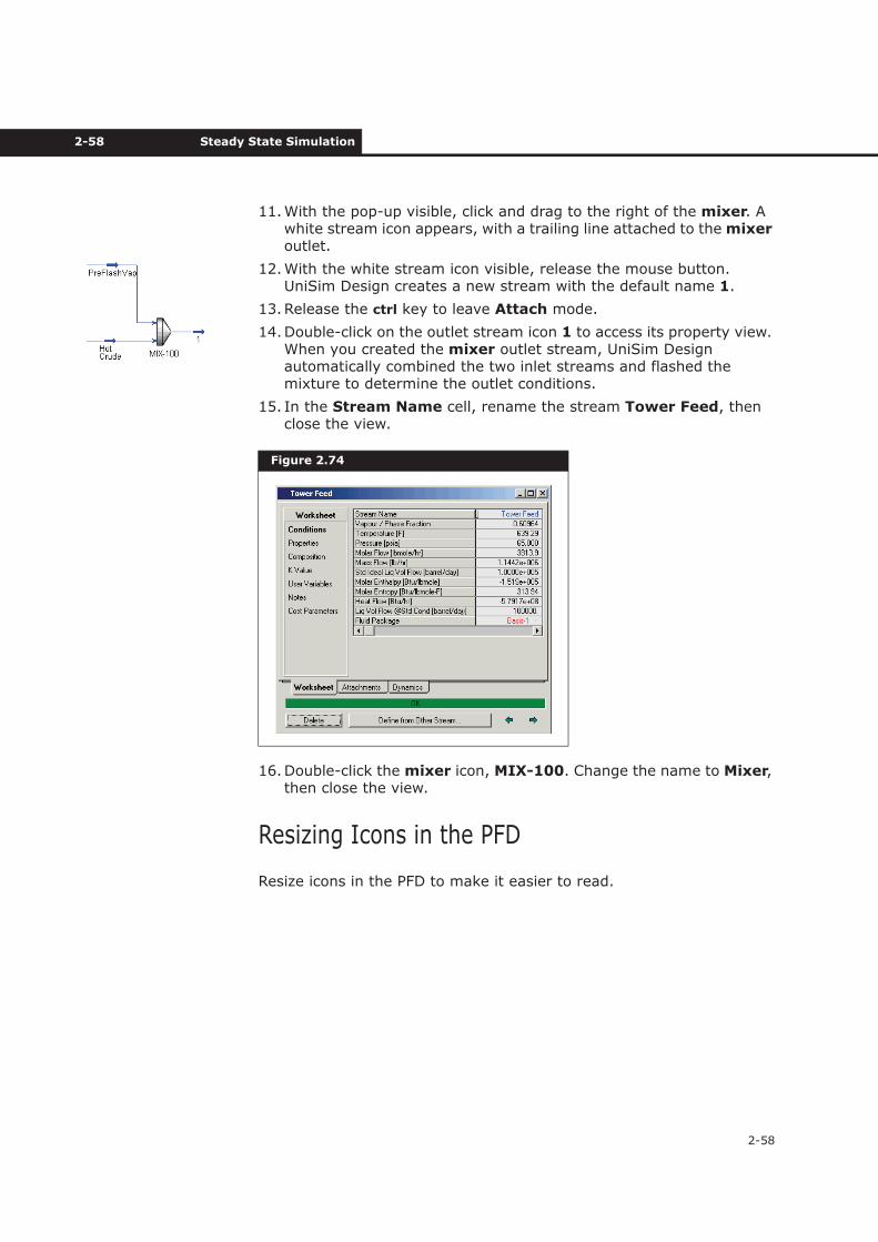
14.Double-click on the outlet stream icon 1 to access its property view. When you created the mixer outlet stream, UniSim Design automatically combined the two inlet streams and flashed the mixture to determine the outlet conditions.
15. In the Stream Name cell, rename the stream Tower Feed, then close the view.
16.Double-click the mixer icon, MIX-100. Change the name to Mixer,then close the view.
Resizing Icons in the PFD
Resize icons in the PFD to make it easier to read.
Figure 2.74
Refining Tutorial 2-59
2-59
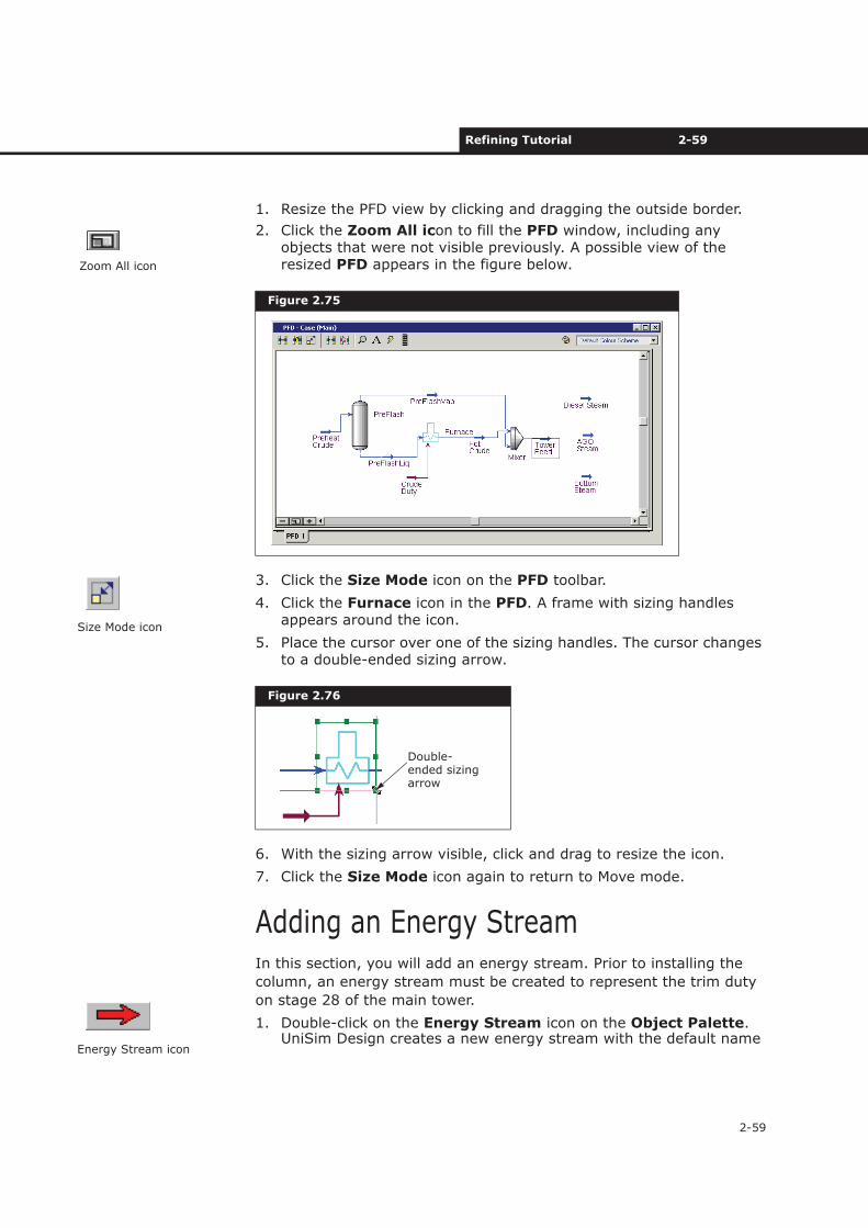
1. Resize the PFD view by clicking and dragging the outside border.
2. Click the Zoom All icon to fill the PFD window, including any objects that were not visible previously. A possible view of the resized PFD appears in the figure below.
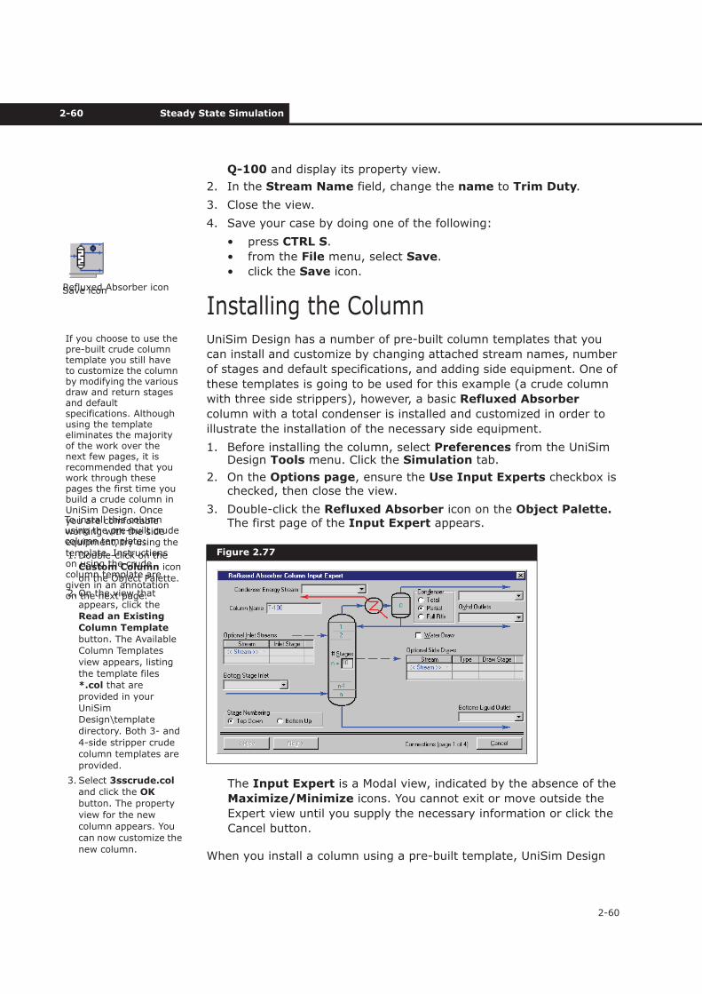
3. Click the Size Mode icon on the PFD toolbar.
4. Click the Furnace icon in the PFD. A frame with sizing handles appears around the icon.
5. Place the cursor over one of the sizing handles. The cursor changes to a double-ended sizing arrow.
6. With the sizing arrow visible, click and drag to resize the icon.
7. Click the Size Mode icon again to return to Move mode.
Adding an Energy StreamIn this section, you will add an energy stream. Prior to installing the
column, an energy stream must be created to represent the trim duty
on stage 28 of the main tower.
1. Double-click on the Energy Stream icon on the Object Palette.UniSim Design creates a new energy stream with the default name
Figure 2.75
Figure 2.76
Zoom All icon
Size Mode icon
Double-ended sizing arrow
Energy Stream icon
2-60 Steady State Simulation
2-60
Q-100 and display its property view.
2. In the Stream Name field, change the name to Trim Duty.
3. Close the view.
4. Save your case by doing one of the following:
• press CTRL S.
• from the File menu, select Save.
• click the Save icon.
Installing the ColumnUniSim Design has a number of pre-built column templates that you
can install and customize by changing attached stream names, number
of stages and default specifications, and adding side equipment. One of
these templates is going to be used for this example (a crude column
with three side strippers), however, a basic Refluxed Absorber
column with a total condenser is installed and customized in order to
illustrate the installation of the necessary side equipment.
1. Before installing the column, select Preferences from the UniSim Design Tools menu. Click the Simulation tab.
2. On the Options page, ensure the Use Input Experts checkbox is checked, then close the view.
3. Double-click the Refluxed Absorber icon on the Object Palette.The first page of the Input Expert appears.
The Input Expert is a Modal view, indicated by the absence of the
Maximize/Minimize icons. You cannot exit or move outside the
Expert view until you supply the necessary information or click the
Cancel button.
When you install a column using a pre-built template, UniSim Design
Figure 2.77
Save icon
If you choose to use the pre-built crude column template you still have to customize the column by modifying the various draw and return stages and default specifications. Although using the template eliminates the majority of the work over the next few pages, it is recommended that you work through these pages the first time you build a crude column in UniSim Design. Once you are comfortable working with the side equipment, try using the template. Instructions on using the crude column template are given in an annotation on the next page.
Refluxed Absorber icon
To install this column using the pre-built crude column template:
1. Double-click on the
Custom Column icon
on the Object Palette.
2. On the view that
appears, click the
Read an Existing
Column Template
button. The Available
Column Templates
view appears, listing
the template files
*.col that are
provided in your
UniSim
Design\template
directory. Both 3- and
4-side stripper crude
column templates are
provided.
3. Select 3sscrude.col
and click the OK
button. The property
view for the new
column appears. You
can now customize the
new column.
Refining Tutorial 2-61
2-61
supplies certain default information, such as the number of stages. The
current active field is # Stages (Number of Stages), indicated by the
thick border inside this field. There are some other points worth noting:
• These are theoretical stages, as the UniSim Design default stage efficiency is one.
• If present, the Condenser and Reboiler are considered separate from the other stages, and are not included in the # Stages field.
Entering Inlet Streams and Number of Trays
For this example, the main column has 29 theoretical stages.
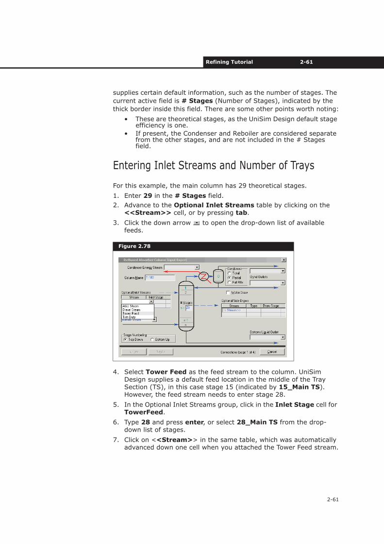
1. Enter 29 in the # Stages field.
2. Advance to the Optional Inlet Streams table by clicking on the <<Stream>> cell, or by pressing tab.
3. Click the down arrow to open the drop-down list of available feeds.
4. Select Tower Feed as the feed stream to the column. UniSim Design supplies a default feed location in the middle of the Tray Section (TS), in this case stage 15 (indicated by 15_Main TS). However, the feed stream needs to enter stage 28.
5. In the Optional Inlet Streams group, click in the Inlet Stage cell for TowerFeed.
6. Type 28 and press enter, or select 28_Main TS from the drop-down list of stages.
7. Click on <<Stream>> in the same table, which was automatically advanced down one cell when you attached the Tower Feed stream.
Figure 2.78
2-62 Steady State Simulation
2-62
8. From the Stream drop-down list, select the Trim Duty stream, which is also fed to stage 28.
9. Advance to the Bottom Stage Inlet field by clicking on it or by pressing tab.
10. In the Bottom Stage Inlet field, click the down arrow to open the drop-down list of available feeds.
11. From the list, select Bottom Steam as the bottom feed for the column.
Entering Outlet Streams
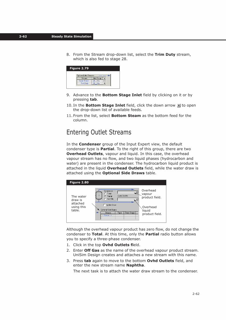
In the Condenser group of the Input Expert view, the default
condenser type is Partial. To the right of this group, there are two
Overhead Outlets, vapour and liquid. In this case, the overhead
vapour stream has no flow, and two liquid phases (hydrocarbon and
water) are present in the condenser. The hydrocarbon liquid product is
attached in the liquid Overhead Outlets field, while the water draw is
attached using the Optional Side Draws table.
Although the overhead vapour product has zero flow, do not change the
condenser to Total. At this time, only the Partial radio button allows
you to specify a three-phase condenser.
1. Click in the top Ovhd Outlets field.
2. Enter Off Gas as the name of the overhead vapour product stream. UniSim Design creates and attaches a new stream with this name.
3. Press tab again to move to the bottom Ovhd Outlets field, and enter the new stream name Naphtha.
The next task is to attach the water draw stream to the condenser.
Figure 2.79
Figure 2.80
Overhead vapour product field.
Overhead liquid product field.
The water draw is attached using this table.
Refining Tutorial 2-63
2-63
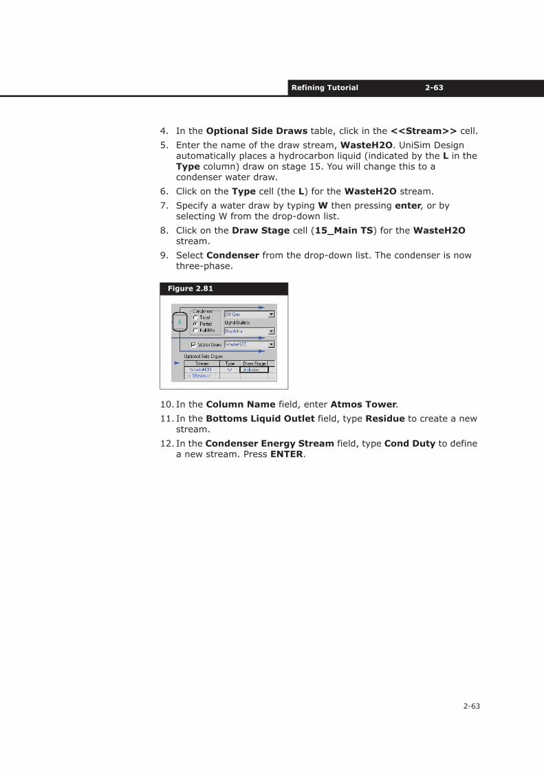
4. In the Optional Side Draws table, click in the <<Stream>> cell.
5. Enter the name of the draw stream, WasteH2O. UniSim Design automatically places a hydrocarbon liquid (indicated by the L in the Type column) draw on stage 15. You will change this to a condenser water draw.
6. Click on the Type cell (the L) for the WasteH2O stream.
7. Specify a water draw by typing W then pressing enter, or by selecting W from the drop-down list.
8. Click on the Draw Stage cell (15_Main TS) for the WasteH2Ostream.
9. Select Condenser from the drop-down list. The condenser is now three-phase.
10. In the Column Name field, enter Atmos Tower.
11. In the Bottoms Liquid Outlet field, type Residue to create a new stream.
12. In the Condenser Energy Stream field, type Cond Duty to define a new stream. Press ENTER.
Figure 2.81
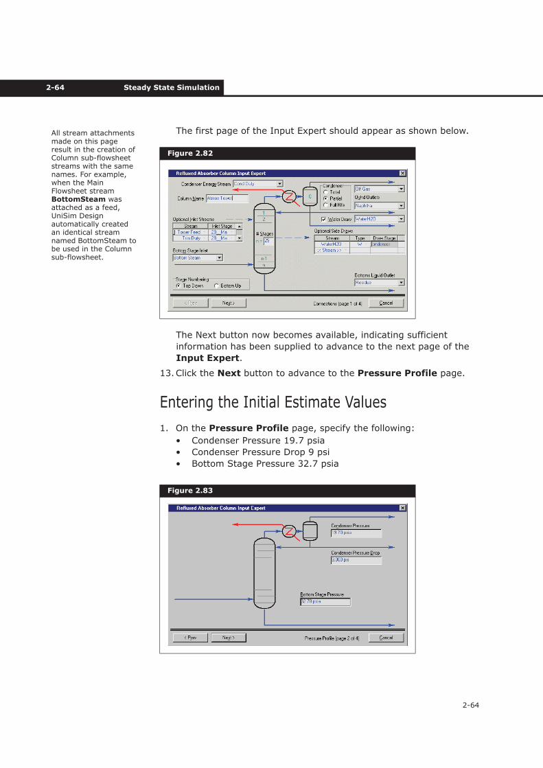
2-64 Steady State Simulation
2-64
The first page of the Input Expert should appear as shown below.
The Next button now becomes available, indicating sufficient
information has been supplied to advance to the next page of the
Input Expert.
13.Click the Next button to advance to the Pressure Profile page.
Entering the Initial Estimate Values
1. On the Pressure Profile page, specify the following:
• Condenser Pressure 19.7 psia
• Condenser Pressure Drop 9 psi
• Bottom Stage Pressure 32.7 psia
Figure 2.82
Figure 2.83
All stream attachments made on this page result in the creation of Column sub-flowsheet streams with the same names. For example, when the Main Flowsheet stream BottomSteam was attached as a feed, UniSim Design automatically created an identical stream named BottomSteam to be used in the Column sub-flowsheet.
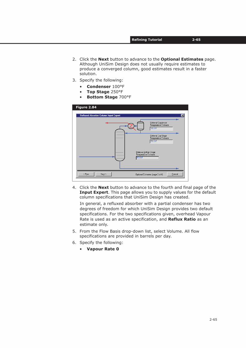
Refining Tutorial 2-65
2-65
2. Click the Next button to advance to the Optional Estimates page. Although UniSim Design does not usually require estimates to produce a converged column, good estimates result in a faster solution.
3. Specify the following:
• Condenser 100°F
• Top Stage 250°F
• Bottom Stage 700°F
4. Click the Next button to advance to the fourth and final page of the Input Expert. This page allows you to supply values for the default column specifications that UniSim Design has created.
In general, a refluxed absorber with a partial condenser has two
degrees of freedom for which UniSim Design provides two default
specifications. For the two specifications given, overhead Vapour
Rate is used as an active specification, and Reflux Ratio as an
estimate only.
5. From the Flow Basis drop-down list, select Volume. All flow specifications are provided in barrels per day.
6. Specify the following:
• Vapour Rate 0
Figure 2.84
2-66 Steady State Simulation
2-66
• Reflux Ratio 1.0.
7. Click the Done button. The Column property view appears.
Adding Specification Values
1. On the Design tab, select the Monitor page.
The main feature of this page is that it displays the status of your
column as it is being calculated, updating information with each
iteration. You can also change specification values, and activate or
de-activate specifications used by the Column solver, directly from
this page.
Figure 2.85
Figure 2.86
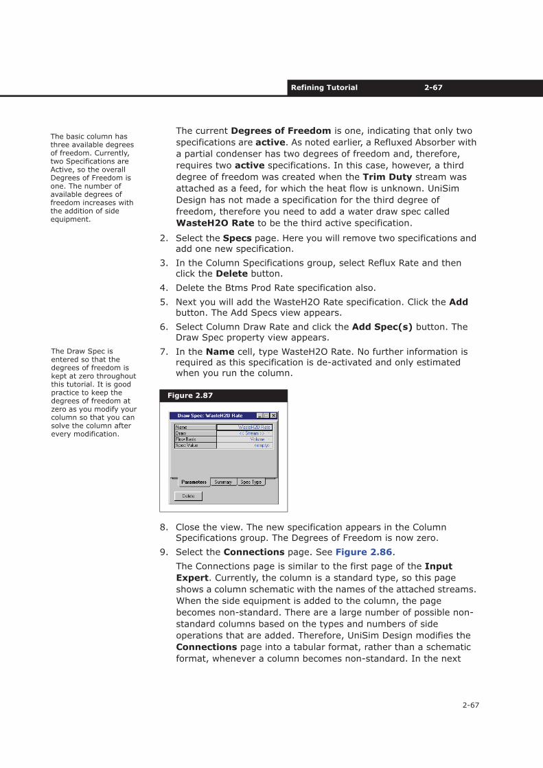
Refining Tutorial 2-67
2-67
The current Degrees of Freedom is one, indicating that only two
specifications are active. As noted earlier, a Refluxed Absorber with
a partial condenser has two degrees of freedom and, therefore,
requires two active specifications. In this case, however, a third
degree of freedom was created when the Trim Duty stream was
attached as a feed, for which the heat flow is unknown. UniSim
Design has not made a specification for the third degree of
freedom, therefore you need to add a water draw spec called
WasteH2O Rate to be the third active specification.
2. Select the Specs page. Here you will remove two specifications and add one new specification.
3. In the Column Specifications group, select Reflux Rate and then click the Delete button.
4. Delete the Btms Prod Rate specification also.
5. Next you will add the WasteH2O Rate specification. Click the Addbutton. The Add Specs view appears.
6. Select Column Draw Rate and click the Add Spec(s) button. The Draw Spec property view appears.
7. In the Name cell, type WasteH2O Rate. No further information is required as this specification is de-activated and only estimated when you run the column.
8. Close the view. The new specification appears in the Column Specifications group. The Degrees of Freedom is now zero.
9. Select the Connections page. See Figure 2.86.
The Connections page is similar to the first page of the Input
Expert. Currently, the column is a standard type, so this page
shows a column schematic with the names of the attached streams.
When the side equipment is added to the column, the page
becomes non-standard. There are a large number of possible non-
standard columns based on the types and numbers of side
operations that are added. Therefore, UniSim Design modifies the
Connections page into a tabular format, rather than a schematic
format, whenever a column becomes non-standard. In the next
Figure 2.87
The basic column has three available degrees of freedom. Currently, two Specifications are Active, so the overall Degrees of Freedom is one. The number of available degrees of freedom increases with the addition of side equipment.
The Draw Spec is entered so that the degrees of freedom is kept at zero throughout this tutorial. It is good practice to keep the degrees of freedom at zero as you modify your column so that you can solve the column after every modification.
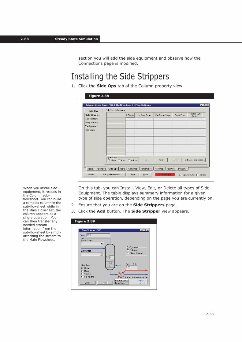
2-68 Steady State Simulation
2-68
section you will add the side equipment and observe how the
Connections page is modified.
Installing the Side Strippers1. Click the Side Ops tab of the Column property view.
On this tab, you can Install, View, Edit, or Delete all types of Side
Equipment. The table displays summary information for a given
type of side operation, depending on the page you are currently on.
2. Ensure that you are on the Side Strippers page.
3. Click the Add button. The Side Stripper view appears.
Figure 2.88
Figure 2.89
When you install side equipment, it resides in the Column sub-flowsheet. You can build a complex column in the sub-flowsheet while in the Main Flowsheet, the column appears as a single operation. You can then transfer any needed stream information from the sub-flowsheet by simply attaching the stream to the Main Flowsheet.
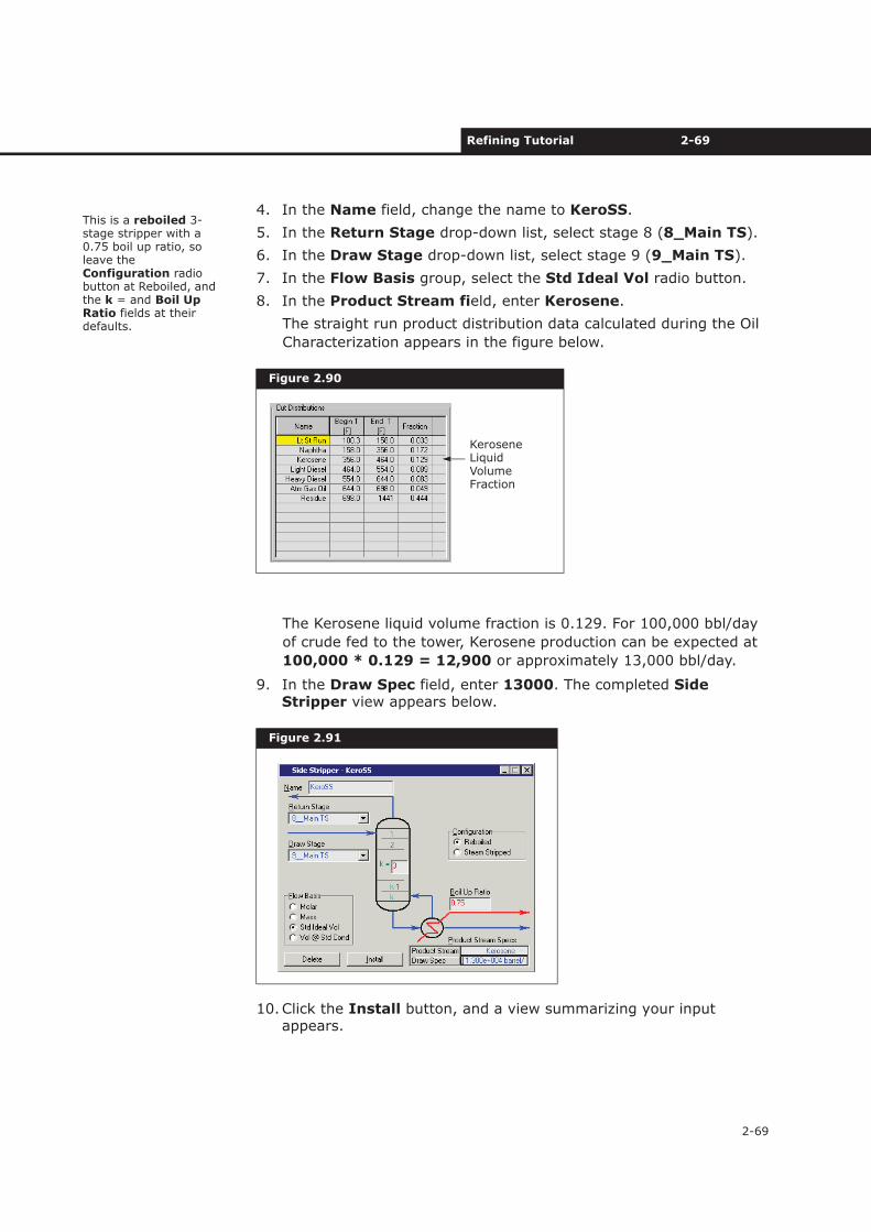
Refining Tutorial 2-69
2-69
4. In the Name field, change the name to KeroSS.
5. In the Return Stage drop-down list, select stage 8 (8_Main TS).
6. In the Draw Stage drop-down list, select stage 9 (9_Main TS).
7. In the Flow Basis group, select the Std Ideal Vol radio button.
8. In the Product Stream field, enter Kerosene.
The straight run product distribution data calculated during the Oil
Characterization appears in the figure below.
The Kerosene liquid volume fraction is 0.129. For 100,000 bbl/day
of crude fed to the tower, Kerosene production can be expected at
100,000 * 0.129 = 12,900 or approximately 13,000 bbl/day.
9. In the Draw Spec field, enter 13000. The completed SideStripper view appears below.
10.Click the Install button, and a view summarizing your input appears.
Figure 2.90
Figure 2.91
This is a reboiled 3-stage stripper with a 0.75 boil up ratio, so leave the Configuration radio button at Reboiled, and the k = and Boil Up Ratio fields at their defaults.
Kerosene LiquidVolume Fraction
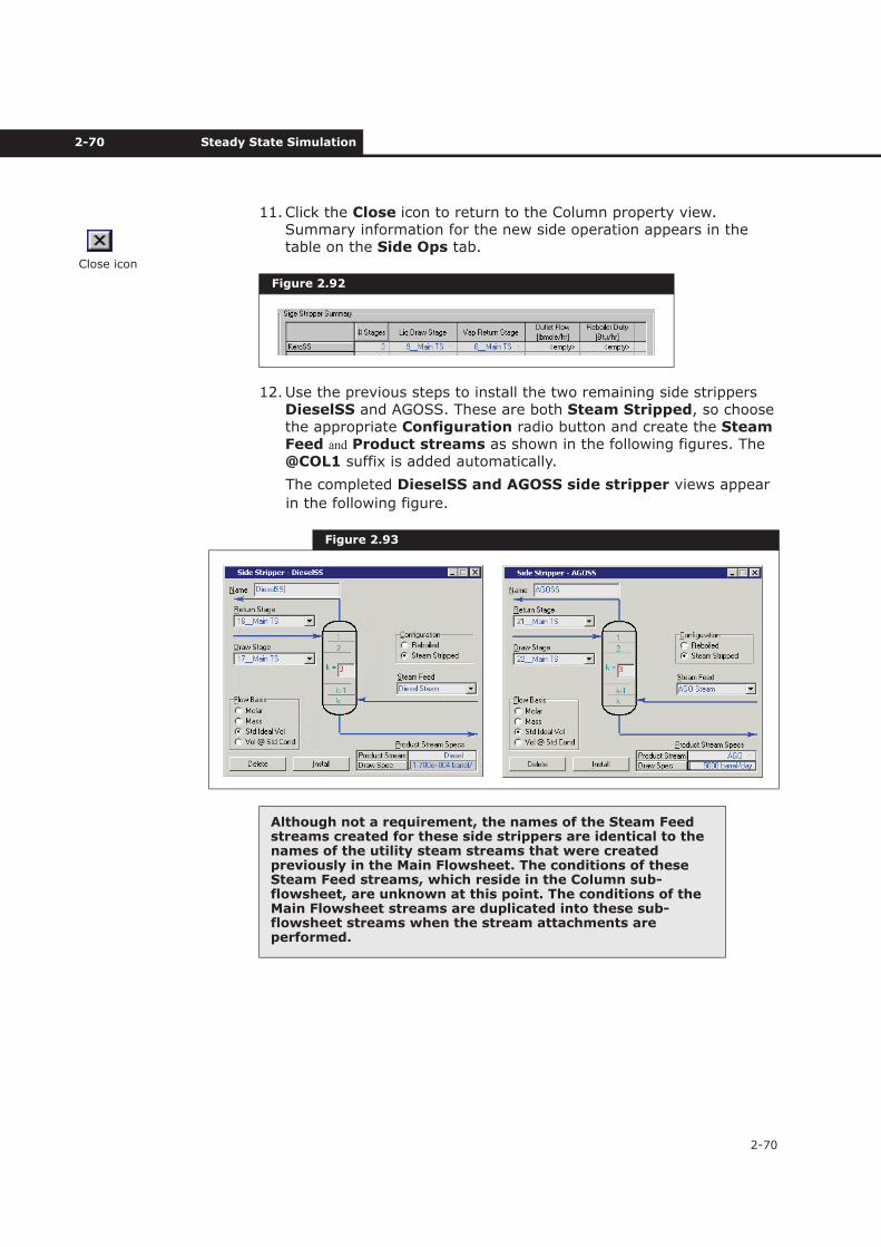
2-70 Steady State Simulation
2-70
11.Click the Close icon to return to the Column property view. Summary information for the new side operation appears in the table on the Side Ops tab.
12.Use the previous steps to install the two remaining side strippers DieselSS and AGOSS. These are both Steam Stripped, so choose the appropriate Configuration radio button and create the Steam Feed and Product streams as shown in the following figures. The @COL1 suffix is added automatically.
The completed DieselSS and AGOSS side stripper views appear
in the following figure.
Figure 2.92
Figure 2.93
Although not a requirement, the names of the Steam Feed streams created for these side strippers are identical to the names of the utility steam streams that were created previously in the Main Flowsheet. The conditions of these Steam Feed streams, which reside in the Column sub-flowsheet, are unknown at this point. The conditions of the Main Flowsheet streams are duplicated into these sub-flowsheet streams when the stream attachments are performed.
Close icon
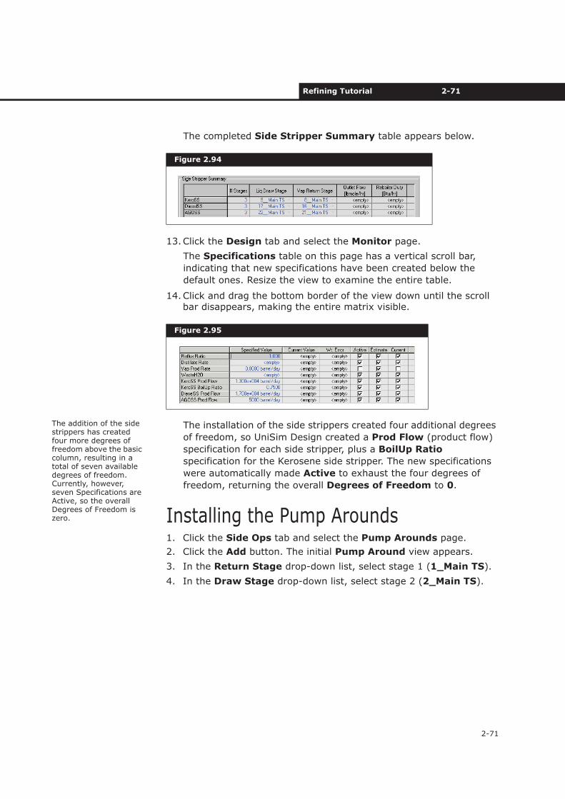
Refining Tutorial 2-71
2-71
The completed Side Stripper Summary table appears below.
13.Click the Design tab and select the Monitor page.
The Specifications table on this page has a vertical scroll bar,
indicating that new specifications have been created below the
default ones. Resize the view to examine the entire table.
14.Click and drag the bottom border of the view down until the scroll bar disappears, making the entire matrix visible.
The installation of the side strippers created four additional degrees
of freedom, so UniSim Design created a Prod Flow (product flow)
specification for each side stripper, plus a BoilUp Ratio
specification for the Kerosene side stripper. The new specifications
were automatically made Active to exhaust the four degrees of
freedom, returning the overall Degrees of Freedom to 0.
Installing the Pump Arounds1. Click the Side Ops tab and select the Pump Arounds page.
2. Click the Add button. The initial Pump Around view appears.
3. In the Return Stage drop-down list, select stage 1 (1_Main TS).
4. In the Draw Stage drop-down list, select stage 2 (2_Main TS).
Figure 2.94
Figure 2.95
The addition of the side strippers has created four more degrees of freedom above the basic column, resulting in a total of seven available degrees of freedom. Currently, however, seven Specifications are Active, so the overall Degrees of Freedom is zero.
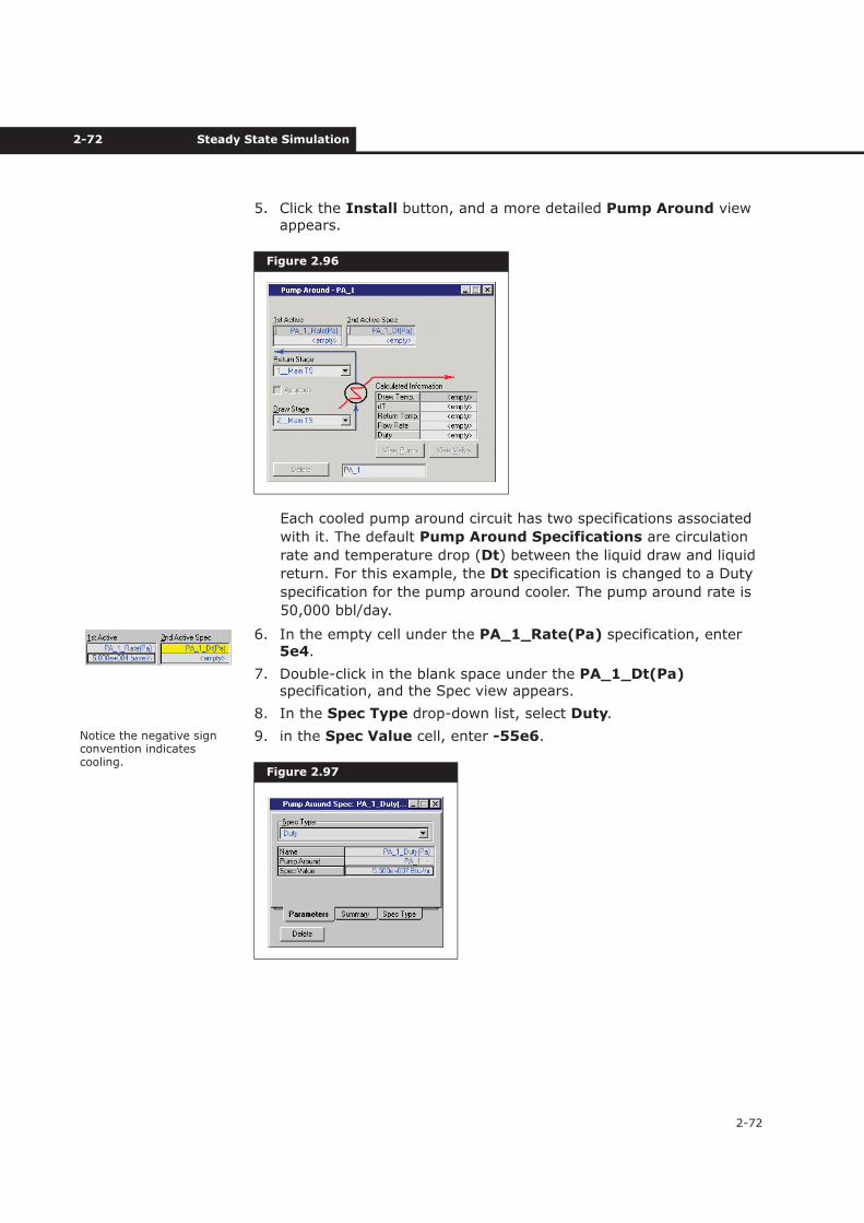
2-72 Steady State Simulation
2-72
5. Click the Install button, and a more detailed Pump Around view appears.
Each cooled pump around circuit has two specifications associated
with it. The default Pump Around Specifications are circulation
rate and temperature drop (Dt) between the liquid draw and liquid
return. For this example, the Dt specification is changed to a Duty
specification for the pump around cooler. The pump around rate is
50,000 bbl/day.
6. In the empty cell under the PA_1_Rate(Pa) specification, enter 5e4.
7. Double-click in the blank space under the PA_1_Dt(Pa) specification, and the Spec view appears.
8. In the Spec Type drop-down list, select Duty.
9. in the Spec Value cell, enter -55e6.
Figure 2.96
Figure 2.97
Notice the negative sign convention indicates cooling.
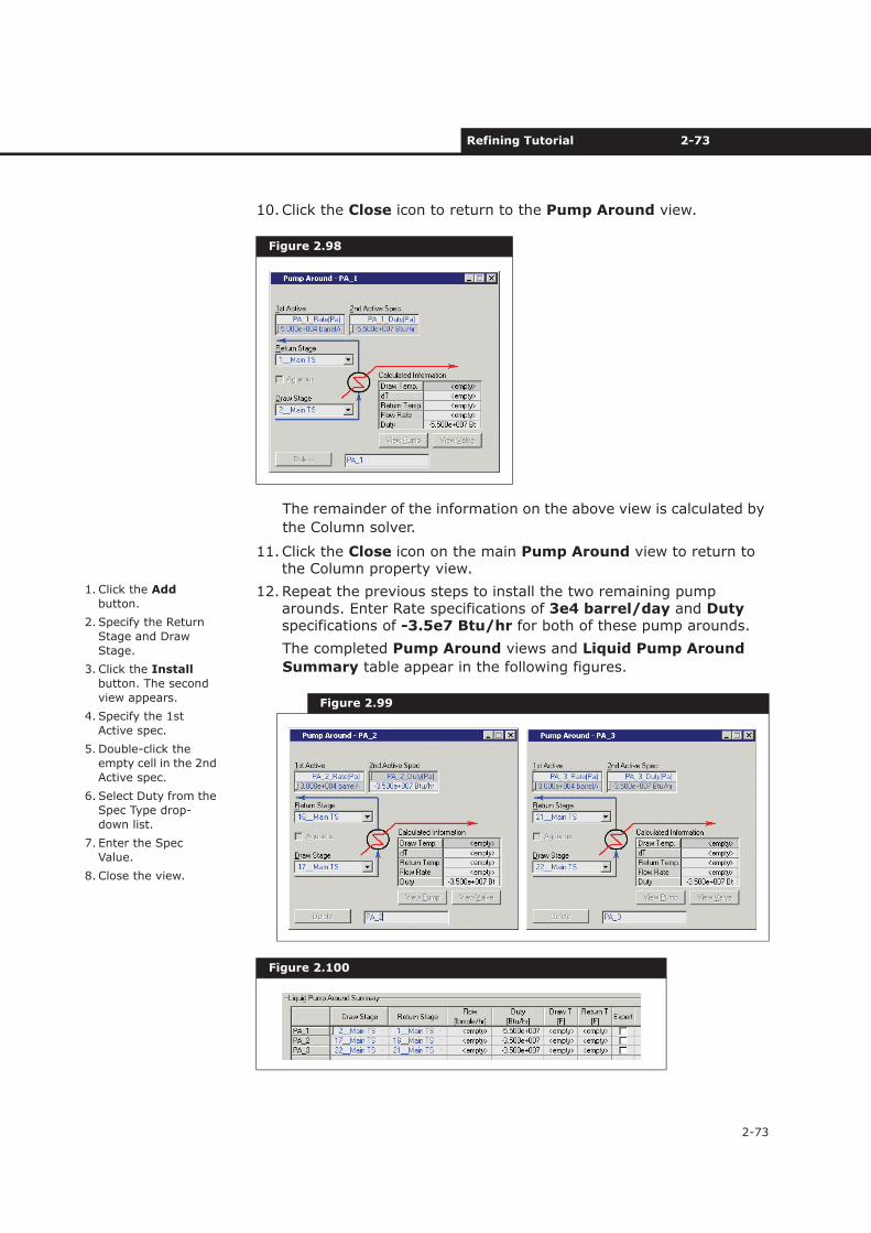
Refining Tutorial 2-73
2-73
10.Click the Close icon to return to the Pump Around view.
The remainder of the information on the above view is calculated by
the Column solver.
11.Click the Close icon on the main Pump Around view to return to the Column property view.
12.Repeat the previous steps to install the two remaining pump arounds. Enter Rate specifications of 3e4 barrel/day and Dutyspecifications of -3.5e7 Btu/hr for both of these pump arounds.
The completed Pump Around views and Liquid Pump Around
Summary table appear in the following figures.
Figure 2.98
Figure 2.99
Figure 2.100
1. Click the Add
button.
2. Specify the Return
Stage and Draw
Stage.
3. Click the Install
button. The second
view appears.
4. Specify the 1st
Active spec.
5. Double-click the
empty cell in the 2nd
Active spec.
6. Select Duty from the
Spec Type drop-
down list.
7. Enter the Spec
Value.
8. Close the view.
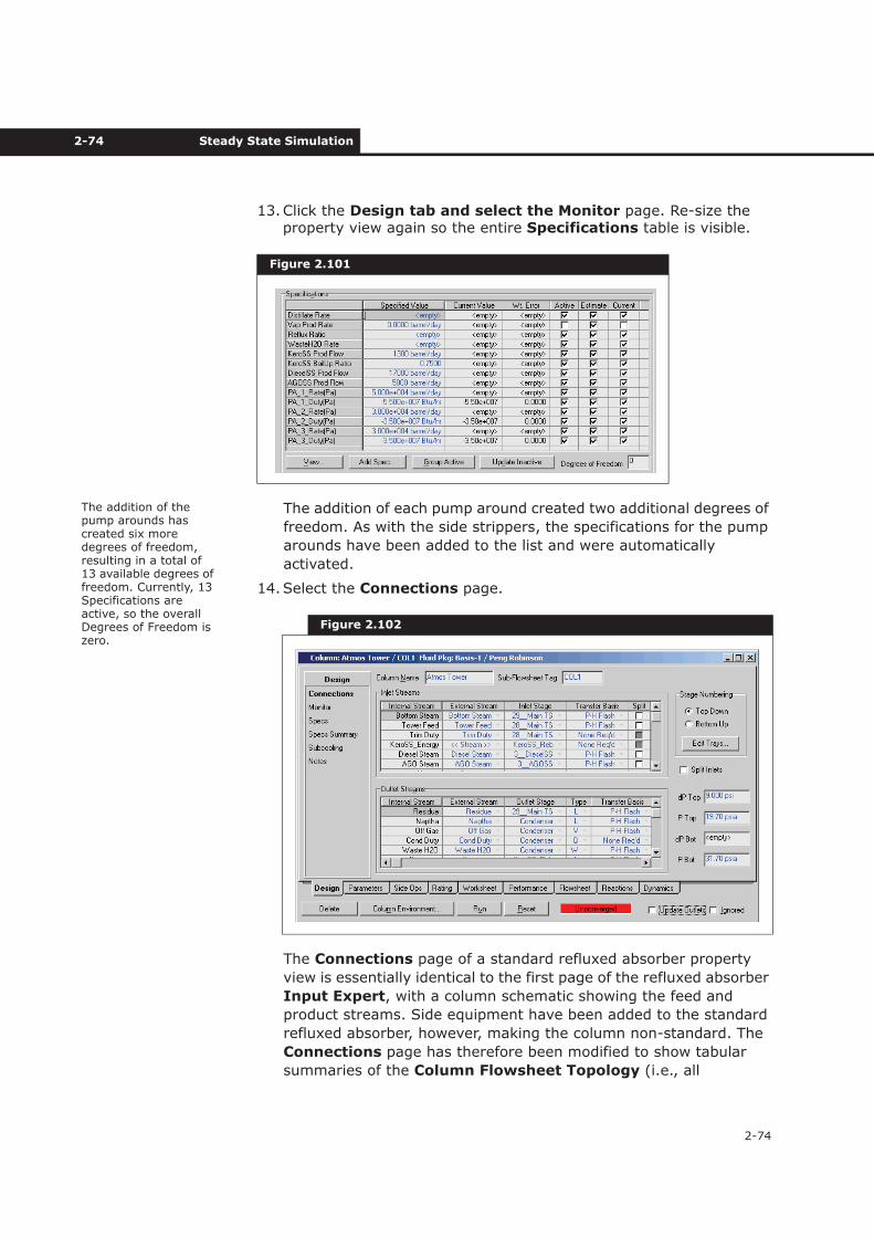
2-74 Steady State Simulation
2-74
13.Click the Design tab and select the Monitor page. Re-size the property view again so the entire Specifications table is visible.
The addition of each pump around created two additional degrees of
freedom. As with the side strippers, the specifications for the pump
arounds have been added to the list and were automatically
activated.
14.Select the Connections page.
The Connections page of a standard refluxed absorber property
view is essentially identical to the first page of the refluxed absorber
Input Expert, with a column schematic showing the feed and
product streams. Side equipment have been added to the standard
refluxed absorber, however, making the column non-standard. The
Connections page has therefore been modified to show tabular
summaries of the Column Flowsheet Topology (i.e., all
Figure 2.101
Figure 2.102
The addition of the pump arounds has created six more degrees of freedom, resulting in a total of 13 available degrees of freedom. Currently, 13 Specifications are active, so the overall Degrees of Freedom is zero.
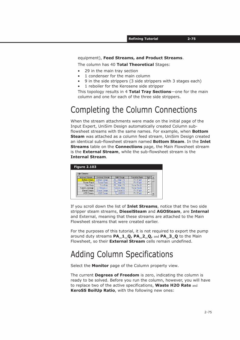
Refining Tutorial 2-75
2-75
equipment), Feed Streams, and Product Streams.
The column has 40 Total Theoretical Stages:
• 29 in the main tray section
• 1 condenser for the main column
• 9 in the side strippers (3 side strippers with 3 stages each)
• 1 reboiler for the Kerosene side stripper
This topology results in 4 Total Tray Sections—one for the main
column and one for each of the three side strippers.
Completing the Column ConnectionsWhen the stream attachments were made on the initial page of the
Input Expert, UniSim Design automatically created Column sub-
flowsheet streams with the same names. For example, when Bottom
Steam was attached as a column feed stream, UniSim Design created
an identical sub-flowsheet stream named Bottom Steam. In the Inlet
Streams table on the Connections page, the Main Flowsheet stream
is the External Stream, while the sub-flowsheet stream is the
Internal Stream.
If you scroll down the list of Inlet Streams, notice that the two side
stripper steam streams, DieselSteam and AGOSteam, are Internal
and External, meaning that these streams are attached to the Main
Flowsheet streams that were created earlier.
For the purposes of this tutorial, it is not required to export the pump
around duty streams PA_1_Q, PA_2_Q, and PA_3_Q to the Main
Flowsheet, so their External Stream cells remain undefined.
Adding Column SpecificationsSelect the Monitor page of the Column property view.
The current Degrees of Freedom is zero, indicating the column is
ready to be solved. Before you run the column, however, you will have
to replace two of the active specifications, Waste H2O Rate and
KeroSS BoilUp Ratio, with the following new ones:
Figure 2.103
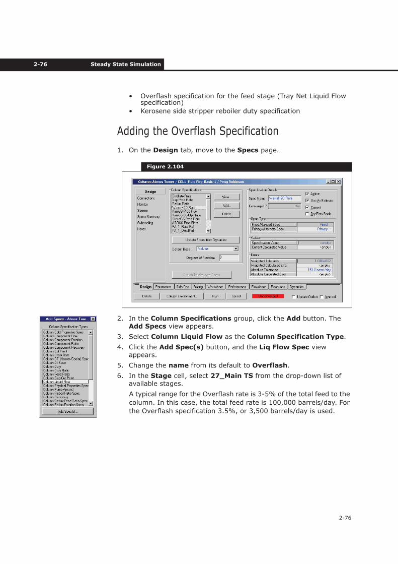
2-76 Steady State Simulation
2-76
• Overflash specification for the feed stage (Tray Net Liquid Flow specification)
• Kerosene side stripper reboiler duty specification
Adding the Overflash Specification
1. On the Design tab, move to the Specs page.
2. In the Column Specifications group, click the Add button. The Add Specs view appears.
3. Select Column Liquid Flow as the Column Specification Type.
4. Click the Add Spec(s) button, and the Liq Flow Spec view appears.
5. Change the name from its default to Overflash.
6. In the Stage cell, select 27_Main TS from the drop-down list of available stages.
A typical range for the Overflash rate is 3-5% of the total feed to the
column. In this case, the total feed rate is 100,000 barrels/day. For
the Overflash specification 3.5%, or 3,500 barrels/day is used.
Figure 2.104
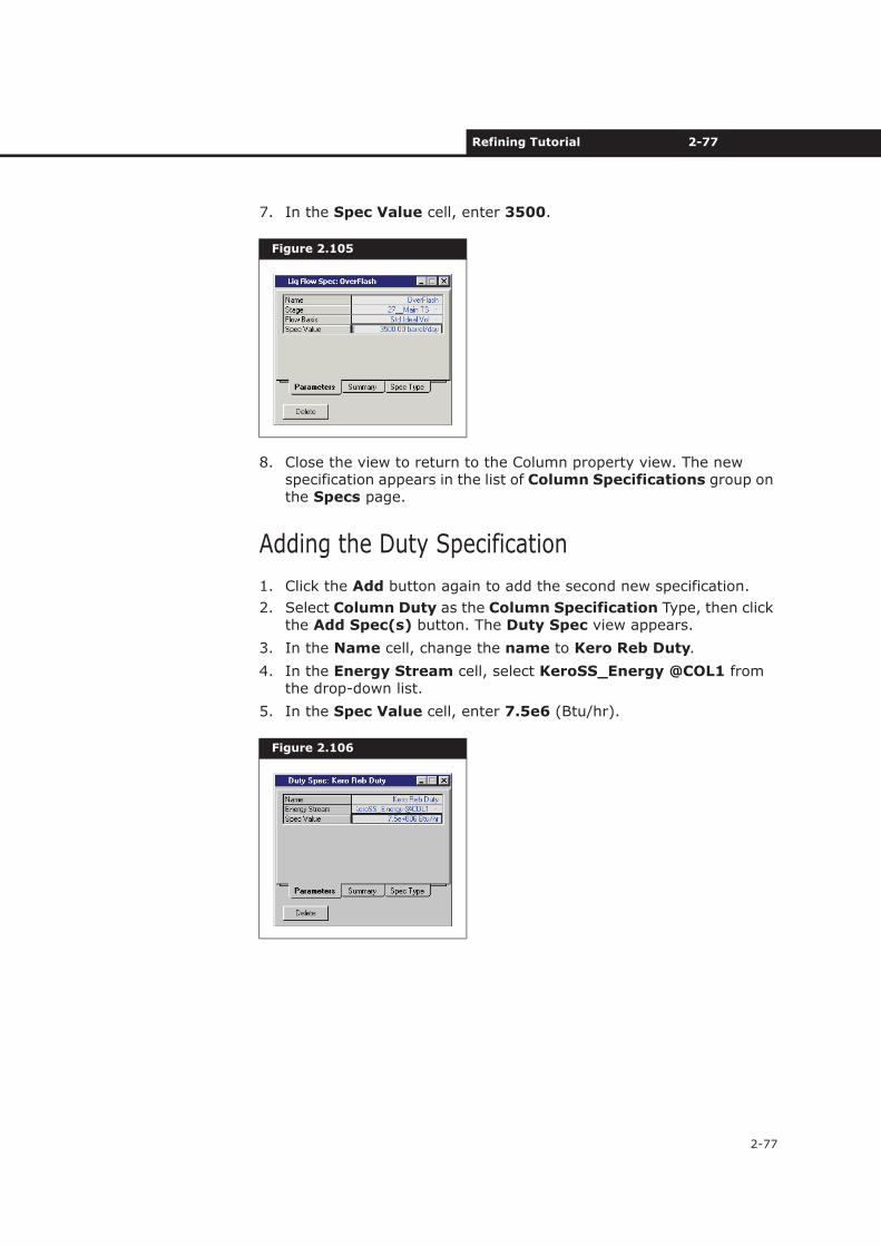
Refining Tutorial 2-77
2-77
7. In the Spec Value cell, enter 3500.
8. Close the view to return to the Column property view. The new specification appears in the list of Column Specifications group on the Specs page.
Adding the Duty Specification
1. Click the Add button again to add the second new specification.
2. Select Column Duty as the Column Specification Type, then click the Add Spec(s) button. The Duty Spec view appears.
3. In the Name cell, change the name to Kero Reb Duty.
4. In the Energy Stream cell, select KeroSS_Energy @COL1 from the drop-down list.
5. In the Spec Value cell, enter 7.5e6 (Btu/hr).
Figure 2.105
Figure 2.106
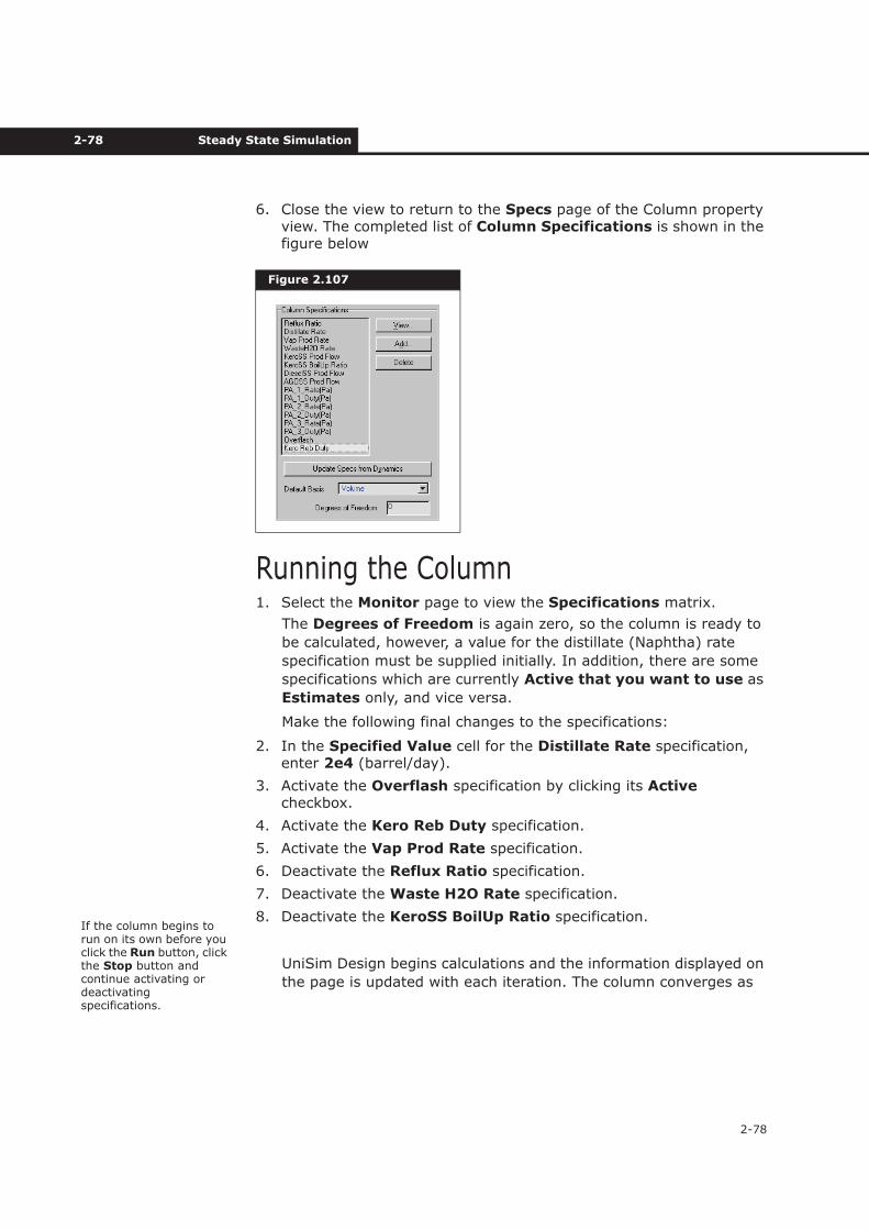
2-78 Steady State Simulation
2-78
6. Close the view to return to the Specs page of the Column property view. The completed list of Column Specifications is shown in the figure below
Running the Column1. Select the Monitor page to view the Specifications matrix.
The Degrees of Freedom is again zero, so the column is ready to
be calculated, however, a value for the distillate (Naphtha) rate
specification must be supplied initially. In addition, there are some
specifications which are currently Active that you want to use as
Estimates only, and vice versa.
Make the following final changes to the specifications:
2. In the Specified Value cell for the Distillate Rate specification, enter 2e4 (barrel/day).
3. Activate the Overflash specification by clicking its Activecheckbox.
4. Activate the Kero Reb Duty specification.
5. Activate the Vap Prod Rate specification.
6. Deactivate the Reflux Ratio specification.
7. Deactivate the Waste H2O Rate specification.
8. Deactivate the KeroSS BoilUp Ratio specification.
UniSim Design begins calculations and the information displayed on
the page is updated with each iteration. The column converges as
Figure 2.107
If the column begins to run on its own before you click the Run button, click the Stop button and continue activating or deactivating specifications.
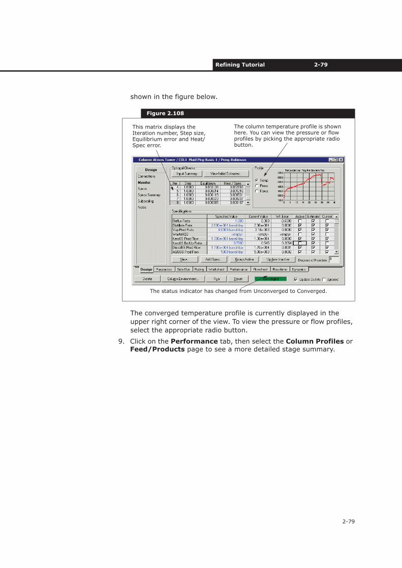
Refining Tutorial 2-79
2-79
shown in the figure below.
The converged temperature profile is currently displayed in the
upper right corner of the view. To view the pressure or flow profiles,
select the appropriate radio button.
9. Click on the Performance tab, then select the Column Profiles or Feed/Products page to see a more detailed stage summary.
Figure 2.108
This matrix displays the Iteration number, Step size, Equilibrium error and Heat/Spec error.
The column temperature profile is shown here. You can view the pressure or flow profiles by picking the appropriate radio button.
The status indicator has changed from Unconverged to Converged.
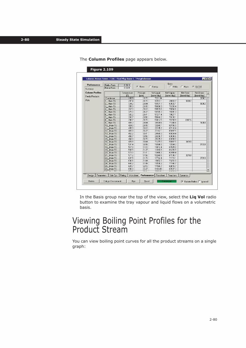
2-80 Steady State Simulation
2-80
The Column Profiles page appears below.
In the Basis group near the top of the view, select the Liq Vol radio
button to examine the tray vapour and liquid flows on a volumetric
basis.
Viewing Boiling Point Profiles for the Product StreamYou can view boiling point curves for all the product streams on a single
graph:
Figure 2.109
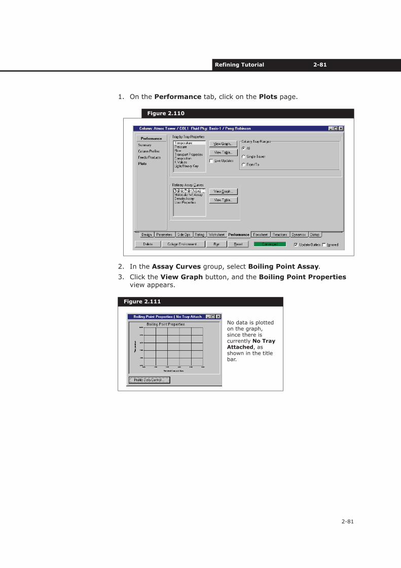
Refining Tutorial 2-81
2-81
1. On the Performance tab, click on the Plots page.
2. In the Assay Curves group, select Boiling Point Assay.
3. Click the View Graph button, and the Boiling Point Propertiesview appears.
Figure 2.110
Figure 2.111
No data is plotted on the graph, since there is currently No Tray Attached, as shown in the title bar.
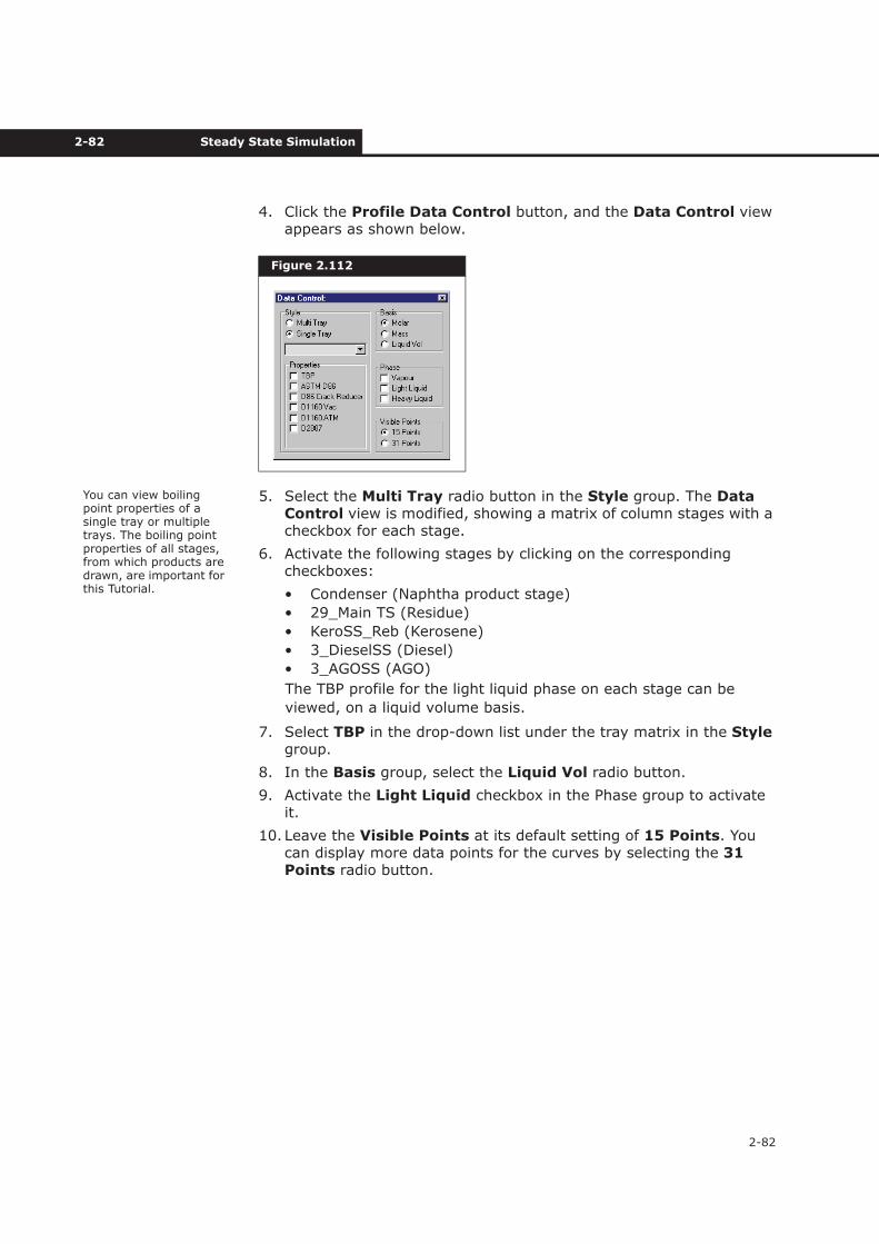
2-82 Steady State Simulation
2-82
4. Click the Profile Data Control button, and the Data Control viewappears as shown below.
5. Select the Multi Tray radio button in the Style group. The Data Control view is modified, showing a matrix of column stages with a checkbox for each stage.
6. Activate the following stages by clicking on the corresponding checkboxes:
• Condenser (Naphtha product stage)
• 29_Main TS (Residue)
• KeroSS_Reb (Kerosene)
• 3_DieselSS (Diesel)
• 3_AGOSS (AGO)
The TBP profile for the light liquid phase on each stage can be
viewed, on a liquid volume basis.
7. Select TBP in the drop-down list under the tray matrix in the Stylegroup.
8. In the Basis group, select the Liquid Vol radio button.
9. Activate the Light Liquid checkbox in the Phase group to activate it.
10. Leave the Visible Points at its default setting of 15 Points. You can display more data points for the curves by selecting the 31 Points radio button.
Figure 2.112
You can view boiling point properties of a single tray or multiple trays. The boiling point properties of all stages, from which products are drawn, are important for this Tutorial.
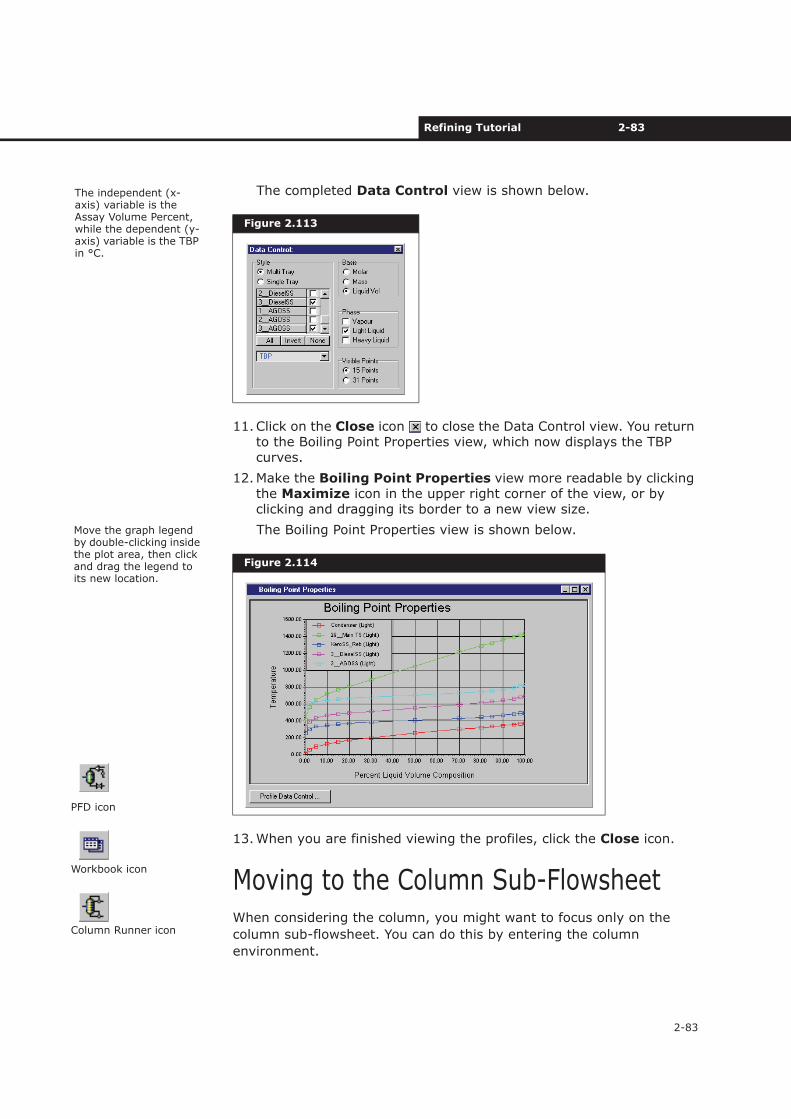
Refining Tutorial 2-83
2-83
The completed Data Control view is shown below.
11.Click on the Close icon to close the Data Control view. You return to the Boiling Point Properties view, which now displays the TBP curves.
12.Make the Boiling Point Properties view more readable by clicking the Maximize icon in the upper right corner of the view, or by clicking and dragging its border to a new view size.
The Boiling Point Properties view is shown below.
13.When you are finished viewing the profiles, click the Close icon.
Moving to the Column Sub-FlowsheetWhen considering the column, you might want to focus only on the
column sub-flowsheet. You can do this by entering the column
environment.
Figure 2.113
Figure 2.114
The independent (x-axis) variable is the Assay Volume Percent, while the dependent (y-axis) variable is the TBP in °C.
Move the graph legend by double-clicking inside the plot area, then click and drag the legend to its new location.
PFD icon
Workbook icon
Column Runner icon
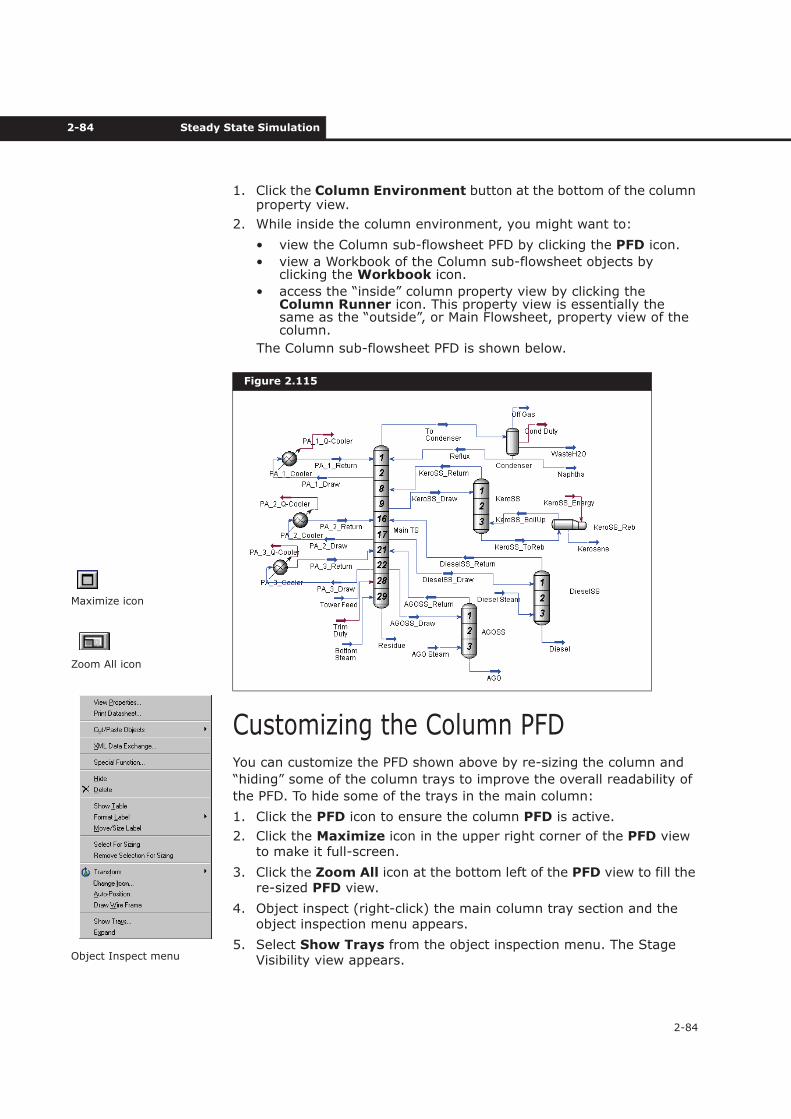
2-84 Steady State Simulation
2-84
1. Click the Column Environment button at the bottom of the column property view.
2. While inside the column environment, you might want to:
• view the Column sub-flowsheet PFD by clicking the PFD icon.
• view a Workbook of the Column sub-flowsheet objects by clicking the Workbook icon.
• access the “inside” column property view by clicking the Column Runner icon. This property view is essentially the same as the “outside”, or Main Flowsheet, property view of the column.
The Column sub-flowsheet PFD is shown below.
Customizing the Column PFDYou can customize the PFD shown above by re-sizing the column and
“hiding” some of the column trays to improve the overall readability of
the PFD. To hide some of the trays in the main column:
1. Click the PFD icon to ensure the column PFD is active.
2. Click the Maximize icon in the upper right corner of the PFD view to make it full-screen.
3. Click the Zoom All icon at the bottom left of the PFD view to fill the re-sized PFD view.
4. Object inspect (right-click) the main column tray section and the object inspection menu appears.
5. Select Show Trays from the object inspection menu. The Stage Visibility view appears.
Figure 2.115
Maximize icon
Zoom All icon
Object Inspect menu
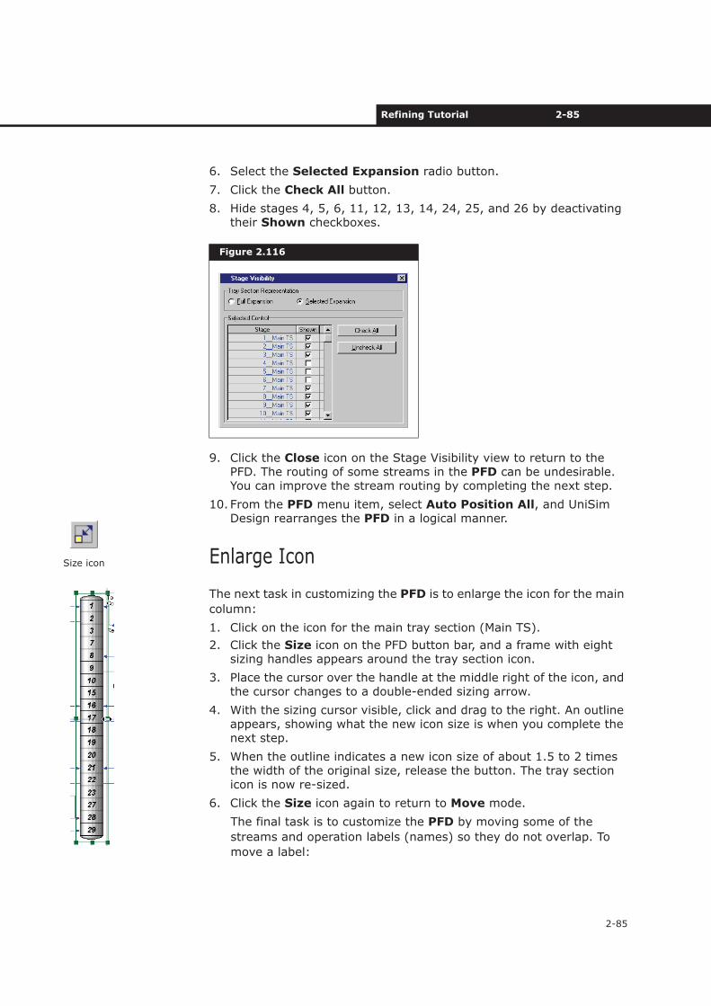
Refining Tutorial 2-85
2-85
6. Select the Selected Expansion radio button.
7. Click the Check All button.
8. Hide stages 4, 5, 6, 11, 12, 13, 14, 24, 25, and 26 by deactivating their Shown checkboxes.
9. Click the Close icon on the Stage Visibility view to return to the PFD. The routing of some streams in the PFD can be undesirable. You can improve the stream routing by completing the next step.
10. From the PFD menu item, select Auto Position All, and UniSim Design rearranges the PFD in a logical manner.
Enlarge Icon
The next task in customizing the PFD is to enlarge the icon for the main
column:
1. Click on the icon for the main tray section (Main TS).
2. Click the Size icon on the PFD button bar, and a frame with eight sizing handles appears around the tray section icon.
3. Place the cursor over the handle at the middle right of the icon, and the cursor changes to a double-ended sizing arrow.
4. With the sizing cursor visible, click and drag to the right. An outline appears, showing what the new icon size is when you complete the next step.
5. When the outline indicates a new icon size of about 1.5 to 2 times the width of the original size, release the button. The tray section icon is now re-sized.
6. Click the Size icon again to return to Move mode.
The final task is to customize the PFD by moving some of the
streams and operation labels (names) so they do not overlap. To
move a label:
Figure 2.116
Size icon
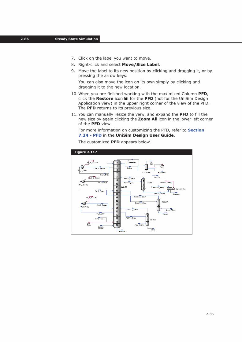
2-86 Steady State Simulation
2-86
7. Click on the label you want to move.
8. Right-click and select Move/Size Label.
9. Move the label to its new position by clicking and dragging it, or by pressing the arrow keys.
You can also move the icon on its own simply by clicking and
dragging it to the new location.
10.When you are finished working with the maximized Column PFD,click the Restore icon for the PFD (not for the UniSim Design Application view) in the upper right corner of the view of the PFD. The PFD returns to its previous size.
11. You can manually resize the view, and expand the PFD to fill the new size by again clicking the Zoom All icon in the lower left corner of the PFD view.
For more information on customizing the PFD, refer to Section
7.24 - PFD in the UniSim Design User Guide.
The customized PFD appears below.
Figure 2.117
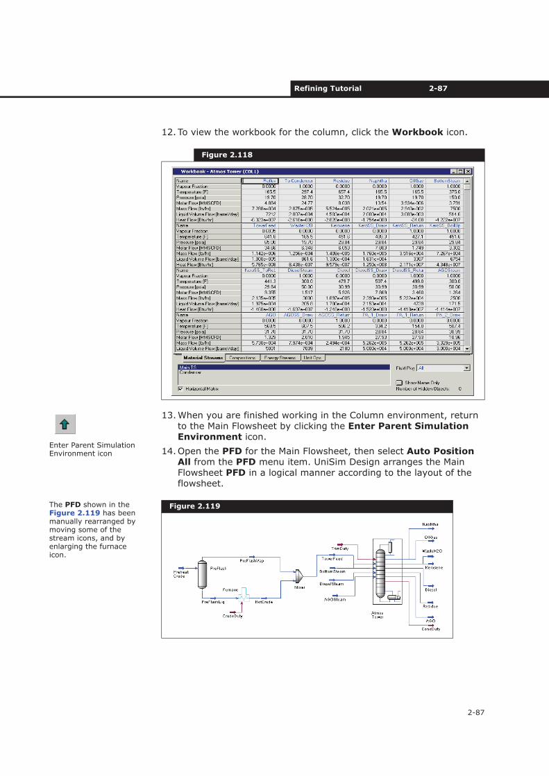
Refining Tutorial 2-87
2-87
12.To view the workbook for the column, click the Workbook icon.
13.When you are finished working in the Column environment, return to the Main Flowsheet by clicking the Enter Parent Simulation Environment icon.
14.Open the PFD for the Main Flowsheet, then select Auto Position All from the PFD menu item. UniSim Design arranges the Main Flowsheet PFD in a logical manner according to the layout of the flowsheet.
Figure 2.118
Figure 2.119
Enter Parent Simulation Environment icon
The PFD shown in the Figure 2.119 has been manually rearranged by moving some of the stream icons, and by enlarging the furnace icon.
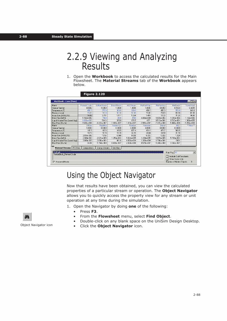
2-88 Steady State Simulation
2-88
2.2.9 Viewing and Analyzing Results
1. Open the Workbook to access the calculated results for the Main Flowsheet. The Material Streams tab of the Workbook appears below.
Using the Object NavigatorNow that results have been obtained, you can view the calculated
properties of a particular stream or operation. The Object Navigator
allows you to quickly access the property view for any stream or unit
operation at any time during the simulation.
1. Open the Navigator by doing one of the following:
• Press F3.
• From the Flowsheet menu, select Find Object.
• Double-click on any blank space on the UniSim Design Desktop.
• Click the Object Navigator icon.
Figure 2.120
Object Navigator icon
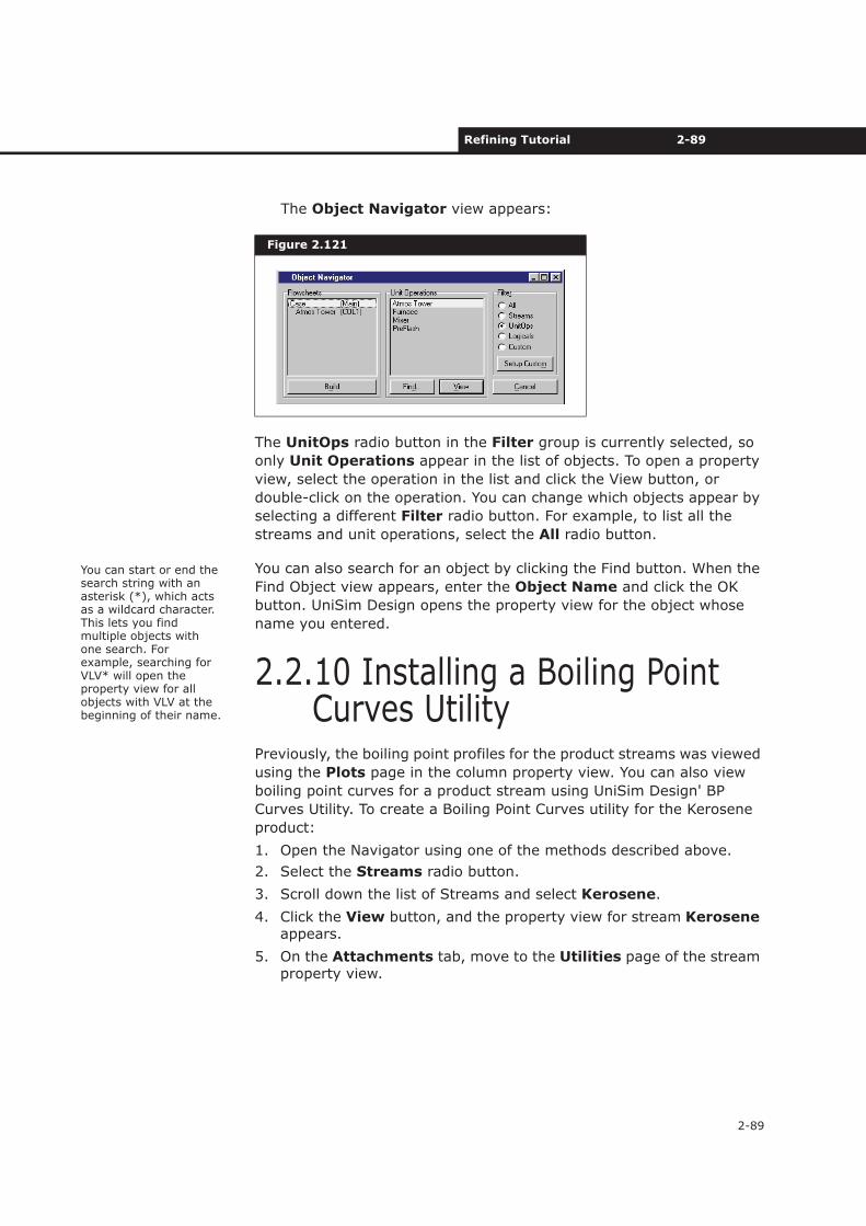
Refining Tutorial 2-89
2-89
The Object Navigator view appears:
The UnitOps radio button in the Filter group is currently selected, so
only Unit Operations appear in the list of objects. To open a property
view, select the operation in the list and click the View button, or
double-click on the operation. You can change which objects appear by
selecting a different Filter radio button. For example, to list all the
streams and unit operations, select the All radio button.
You can also search for an object by clicking the Find button. When the
Find Object view appears, enter the Object Name and click the OK
button. UniSim Design opens the property view for the object whose
name you entered.
2.2.10 Installing a Boiling Point Curves Utility
Previously, the boiling point profiles for the product streams was viewed
using the Plots page in the column property view. You can also view
boiling point curves for a product stream using UniSim Design' BP
Curves Utility. To create a Boiling Point Curves utility for the Kerosene
product:
1. Open the Navigator using one of the methods described above.
2. Select the Streams radio button.
3. Scroll down the list of Streams and select Kerosene.
4. Click the View button, and the property view for stream Keroseneappears.
5. On the Attachments tab, move to the Utilities page of the stream property view.
Figure 2.121
You can start or end the search string with an asterisk (*), which acts as a wildcard character. This lets you find multiple objects with one search. For example, searching for VLV* will open the property view for all objects with VLV at the beginning of their name.
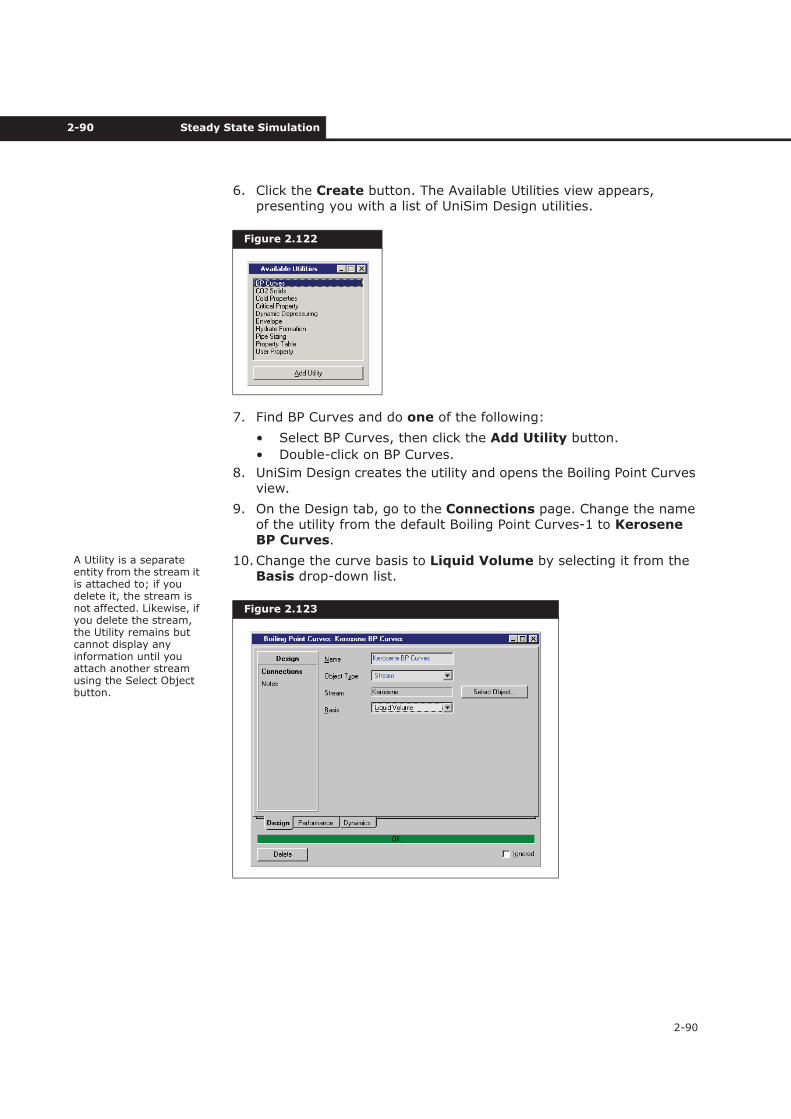
2-90 Steady State Simulation
2-90
6. Click the Create button. The Available Utilities view appears, presenting you with a list of UniSim Design utilities.
7. Find BP Curves and do one of the following:
• Select BP Curves, then click the Add Utility button.
• Double-click on BP Curves.
8. UniSim Design creates the utility and opens the Boiling Point Curves view.
9. On the Design tab, go to the Connections page. Change the name of the utility from the default Boiling Point Curves-1 to KeroseneBP Curves.
10.Change the curve basis to Liquid Volume by selecting it from the Basis drop-down list.
Figure 2.122
Figure 2.123
A Utility is a separate entity from the stream it is attached to; if you delete it, the stream is not affected. Likewise, if you delete the stream, the Utility remains but cannot display any information until you attach another stream using the Select Object button.
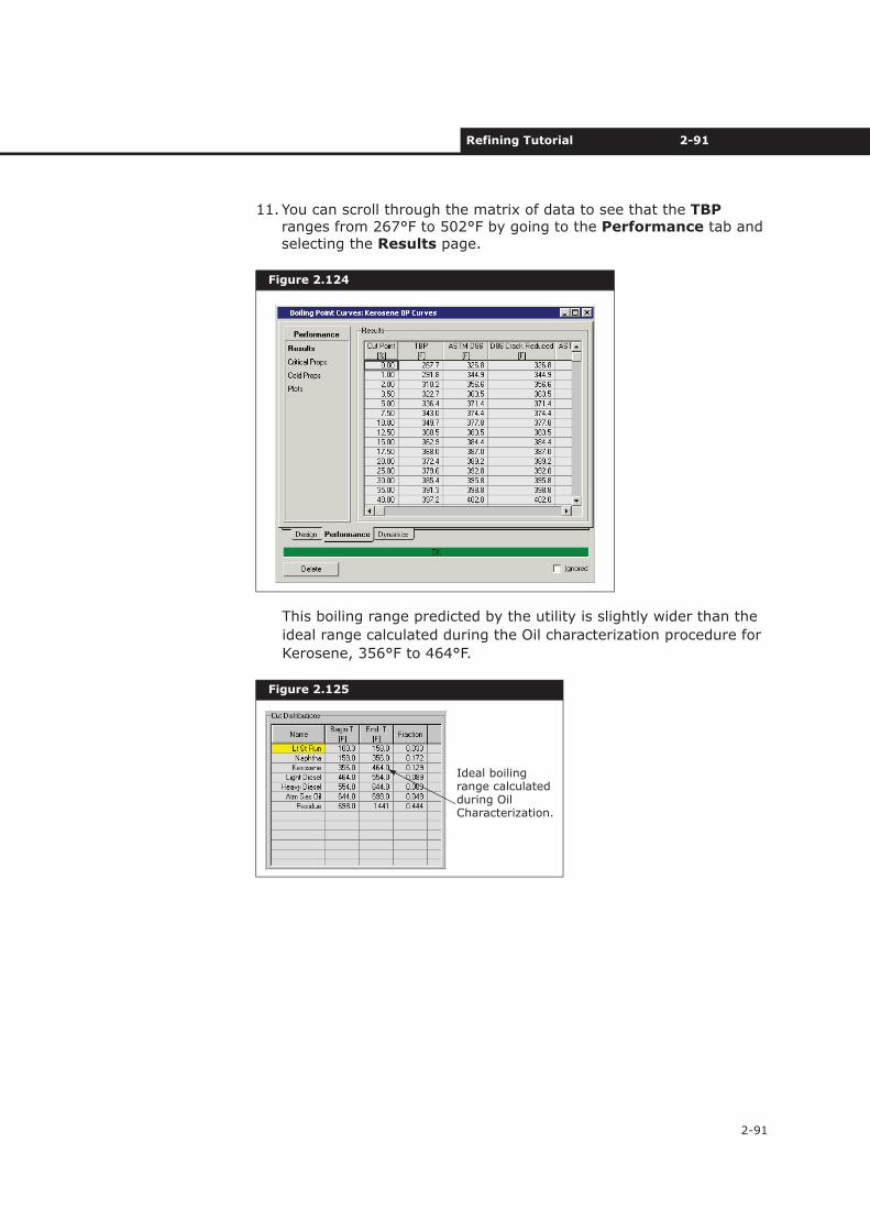
Refining Tutorial 2-91
2-91
11.You can scroll through the matrix of data to see that the TBPranges from 267°F to 502°F by going to the Performance tab and selecting the Results page.
This boiling range predicted by the utility is slightly wider than the
ideal range calculated during the Oil characterization procedure for
Kerosene, 356°F to 464°F.
Figure 2.124
Figure 2.125
Ideal boiling range calculated during Oil Characterization.
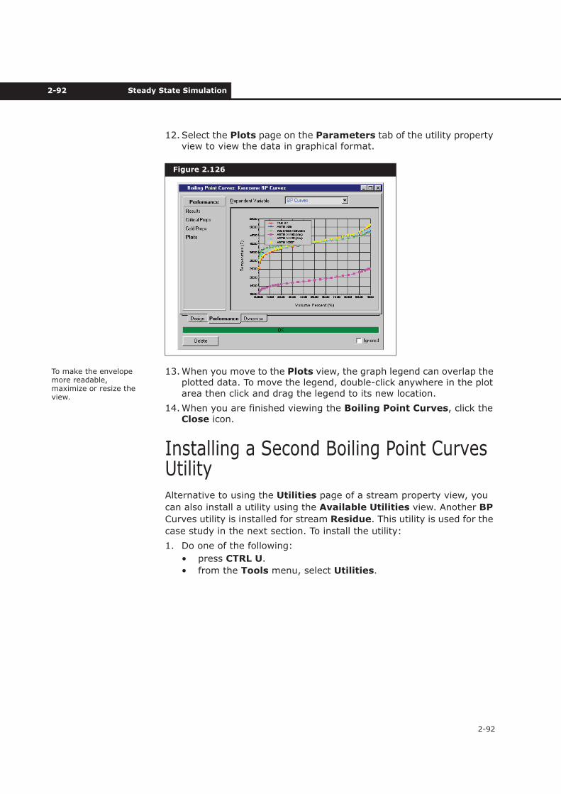
2-92 Steady State Simulation
2-92
12.Select the Plots page on the Parameters tab of the utility property view to view the data in graphical format.
13.When you move to the Plots view, the graph legend can overlap the plotted data. To move the legend, double-click anywhere in the plot area then click and drag the legend to its new location.
14.When you are finished viewing the Boiling Point Curves, click the Close icon.
Installing a Second Boiling Point Curves UtilityAlternative to using the Utilities page of a stream property view, you
can also install a utility using the Available Utilities view. Another BP
Curves utility is installed for stream Residue. This utility is used for the
case study in the next section. To install the utility:
1. Do one of the following:
• press CTRL U.
• from the Tools menu, select Utilities.
Figure 2.126
To make the envelope more readable, maximize or resize the view.
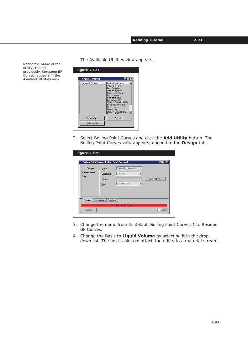
Refining Tutorial 2-93
2-93
The Available Utilities view appears.
2. Select Boiling Point Curves and click the Add Utility button. The Boiling Point Curves view appears, opened to the Design tab.
3. Change the name from its default Boiling Point Curves-1 to Residue BP Curves.
4. Change the Basis to Liquid Volume by selecting it in the drop-down list. The next task is to attach the utility to a material stream.
Figure 2.127
Figure 2.128
Notice the name of the utility created previously, Kerosene BP Curves, appears in the Available Utilities view.
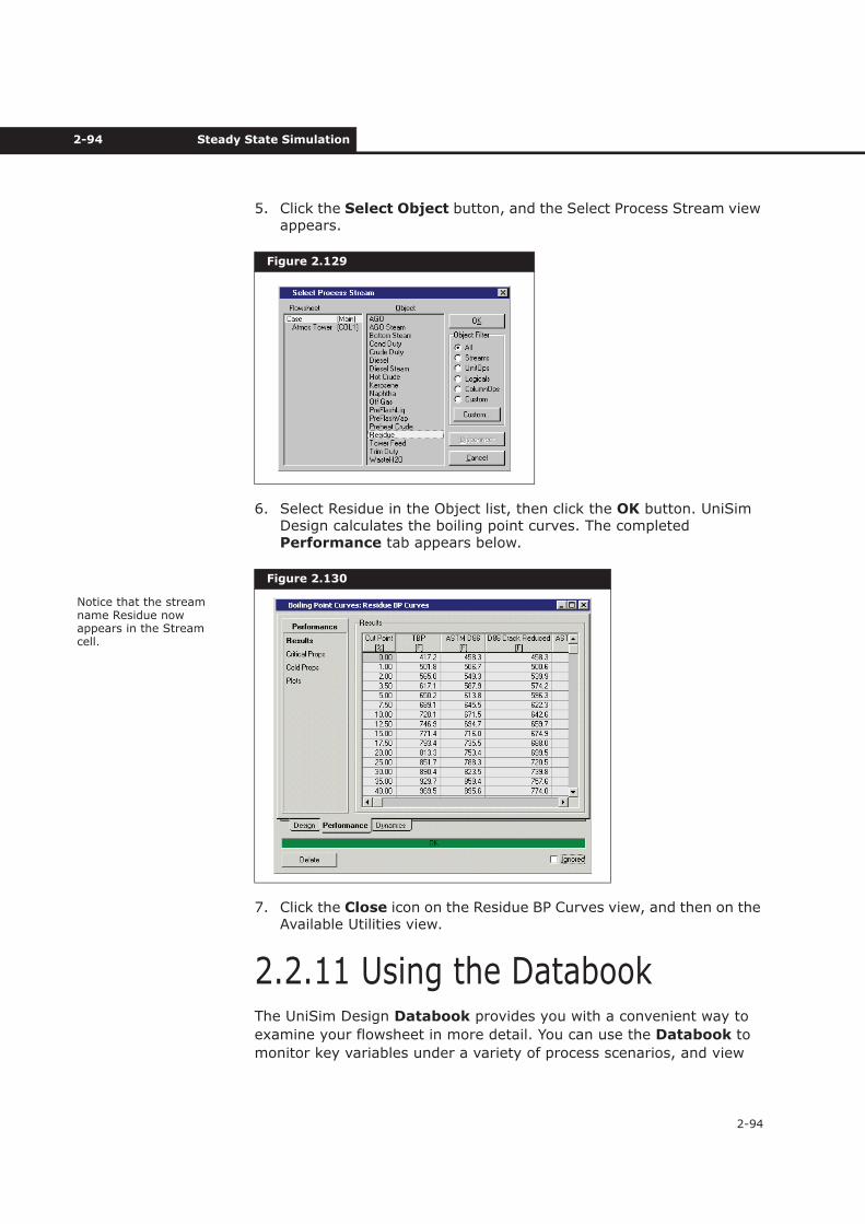
2-94 Steady State Simulation
2-94
5. Click the Select Object button, and the Select Process Stream view appears.
6. Select Residue in the Object list, then click the OK button. UniSim Design calculates the boiling point curves. The completed Performance tab appears below.
7. Click the Close icon on the Residue BP Curves view, and then on the Available Utilities view.
2.2.11 Using the DatabookThe UniSim Design Databook provides you with a convenient way to
examine your flowsheet in more detail. You can use the Databook to
monitor key variables under a variety of process scenarios, and view
Figure 2.129
Figure 2.130
Notice that the stream name Residue now appears in the Stream cell.
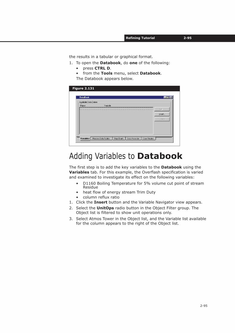
Refining Tutorial 2-95
2-95
the results in a tabular or graphical format.
1. To open the Databook, do one of the following:
• press CTRL D.
• from the Tools menu, select Databook.
The Databook appears below.
Adding Variables to DatabookThe first step is to add the key variables to the Databook using the
Variables tab. For this example, the Overflash specification is varied
and examined to investigate its effect on the following variables:
• D1160 Boiling Temperature for 5% volume cut point of stream Residue
• heat flow of energy stream Trim Duty
• column reflux ratio
1. Click the Insert button and the Variable Navigator view appears.
2. Select the UnitOps radio button in the Object Filter group. The Object list is filtered to show unit operations only.
3. Select Atmos Tower in the Object list, and the Variable list available for the column appears to the right of the Object list.
Figure 2.131
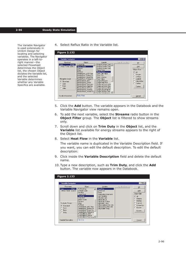
2-96 Steady State Simulation
2-96
4. Select Reflux Ratio in the Variable list.
5. Click the Add button. The variable appears in the Databook and the Variable Navigator view remains open.
6. To add the next variable, select the Streams radio button in the Object Filter group. The Object list is filtered to show streams only.
7. Scroll down and click on Trim Duty in the Object list, and the Variable list available for energy streams appears to the right of the Object list.
8. Select Heat Flow in the Variable list.
The variable name is duplicated in the Variable Description field. If
you want, you can edit the default description. To edit the default
description:
9. Click inside the Variable Description field and delete the default name.
10. Type a new description, such as Trim Duty, and click the Addbutton. The variable now appears in the Databook.
Figure 2.132
Figure 2.133
The Variable Navigator is used extensively in UniSim Design for locating and selecting variables. The Navigator operates in a left-to-right manner—the selected Flowsheet determines the Object list, the chosen Object dictates the Variable list, and the selected Variable determines whether any Variable Specifics are available.
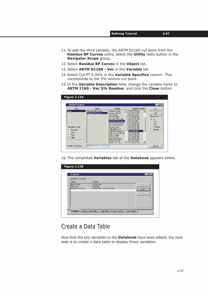
Refining Tutorial 2-97
2-97
11.To add the third variable, the ASTM D1160 cut point from the Residue BP Curves utility, select the Utility radio button in the Navigator Scope group.
12.Select Residue BP Curves in the Object list.
13.Select ASTM D1160 - Vac in the Variable list.
14.Select Cut PT-5.00% in the Variable Specifics column. This corresponds to the 5% volume cut point.
15. In the Variable Description field, change the variable name to ASTM 1160 - Vac 5% Residue, and click the Close button.
16. The completed Variables tab of the Databook appears below.
Create a Data Table
Now that the key variables to the Databook have been added, the next
task is to create a data table to display those variables:
Figure 2.134
Figure 2.135
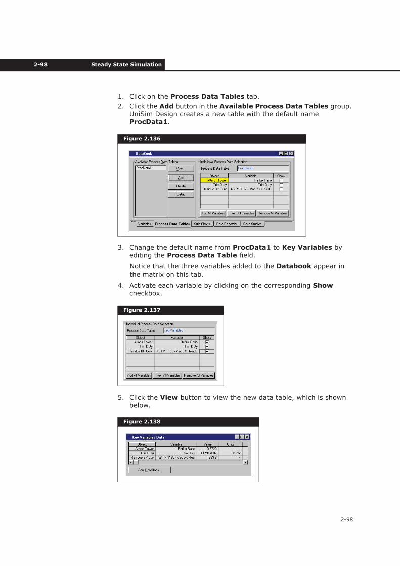
2-98 Steady State Simulation
2-98
1. Click on the Process Data Tables tab.
2. Click the Add button in the Available Process Data Tables group. UniSim Design creates a new table with the default name ProcData1.
3. Change the default name from ProcData1 to Key Variables by editing the Process Data Table field.
Notice that the three variables added to the Databook appear in
the matrix on this tab.
4. Activate each variable by clicking on the corresponding Showcheckbox.
5. Click the View button to view the new data table, which is shown below.
Figure 2.136
Figure 2.137
Figure 2.138
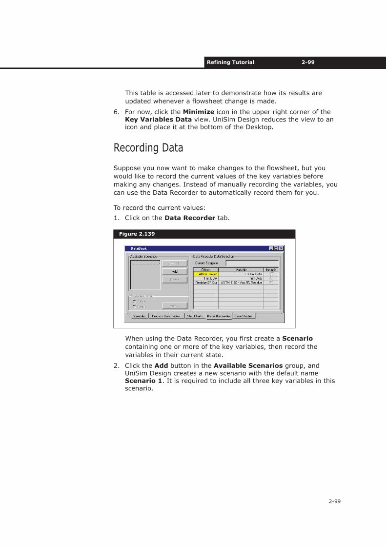
Refining Tutorial 2-99
2-99
This table is accessed later to demonstrate how its results are
updated whenever a flowsheet change is made.
6. For now, click the Minimize icon in the upper right corner of the Key Variables Data view. UniSim Design reduces the view to an icon and place it at the bottom of the Desktop.
Recording Data
Suppose you now want to make changes to the flowsheet, but you
would like to record the current values of the key variables before
making any changes. Instead of manually recording the variables, you
can use the Data Recorder to automatically record them for you.
To record the current values:
1. Click on the Data Recorder tab.
When using the Data Recorder, you first create a Scenario
containing one or more of the key variables, then record the
variables in their current state.
2. Click the Add button in the Available Scenarios group, and UniSim Design creates a new scenario with the default name Scenario 1. It is required to include all three key variables in this scenario.
Figure 2.139
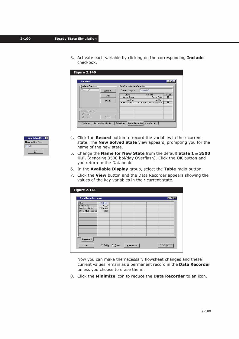
2-100 Steady State Simulation
2-100
3. Activate each variable by clicking on the corresponding Includecheckbox.
4. Click the Record button to record the variables in their current state. The New Solved State view appears, prompting you for the name of the new state.
5. Change the Name for New State from the default State 1 to 3500 O.F. (denoting 3500 bbl/day Overflash). Click the OK button and you return to the Databook.
6. In the Available Display group, select the Table radio button.
7. Click the View button and the Data Recorder appears showing the values of the key variables in their current state.
Now you can make the necessary flowsheet changes and these
current values remain as a permanent record in the Data Recorder
unless you choose to erase them.
8. Click the Minimize icon to reduce the Data Recorder to an icon.
Figure 2.140
Figure 2.141
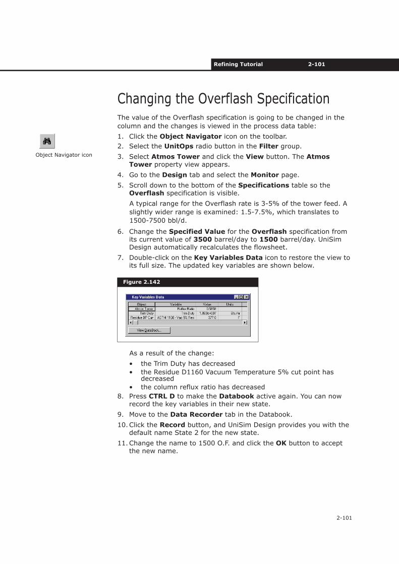
Refining Tutorial 2-101
2-101
Changing the Overflash SpecificationThe value of the Overflash specification is going to be changed in the
column and the changes is viewed in the process data table:
1. Click the Object Navigator icon on the toolbar.
2. Select the UnitOps radio button in the Filter group.
3. Select Atmos Tower and click the View button. The Atmos Tower property view appears.
4. Go to the Design tab and select the Monitor page.
5. Scroll down to the bottom of the Specifications table so the Overflash specification is visible.
A typical range for the Overflash rate is 3-5% of the tower feed. A
slightly wider range is examined: 1.5-7.5%, which translates to
1500-7500 bbl/d.
6. Change the Specified Value for the Overflash specification from its current value of 3500 barrel/day to 1500 barrel/day. UniSim Design automatically recalculates the flowsheet.
7. Double-click on the Key Variables Data icon to restore the view to its full size. The updated key variables are shown below.
As a result of the change:
• the Trim Duty has decreased
• the Residue D1160 Vacuum Temperature 5% cut point has decreased
• the column reflux ratio has decreased
8. Press CTRL D to make the Databook active again. You can now record the key variables in their new state.
9. Move to the Data Recorder tab in the Databook.
10.Click the Record button, and UniSim Design provides you with the default name State 2 for the new state.
11.Change the name to 1500 O.F. and click the OK button to accept the new name.
Figure 2.142
Object Navigator icon
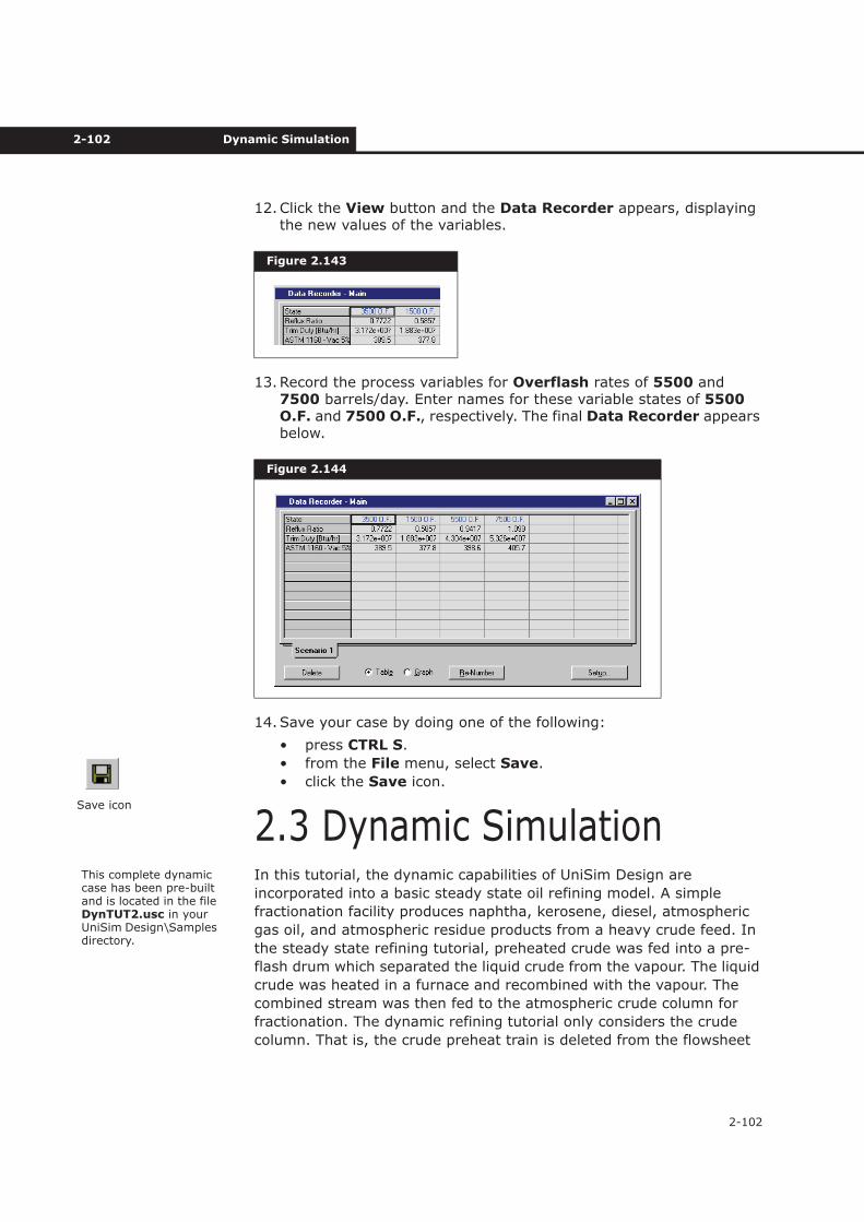
2-102 Dynamic Simulation
2-102
12.Click the View button and the Data Recorder appears, displaying the new values of the variables.
13.Record the process variables for Overflash rates of 5500 and 7500 barrels/day. Enter names for these variable states of 5500 O.F. and 7500 O.F., respectively. The final Data Recorder appears below.
14.Save your case by doing one of the following:
• press CTRL S.
• from the File menu, select Save.
• click the Save icon.
2.3 Dynamic SimulationIn this tutorial, the dynamic capabilities of UniSim Design are
incorporated into a basic steady state oil refining model. A simple
fractionation facility produces naphtha, kerosene, diesel, atmospheric
gas oil, and atmospheric residue products from a heavy crude feed. In
the steady state refining tutorial, preheated crude was fed into a pre-
flash drum which separated the liquid crude from the vapour. The liquid
crude was heated in a furnace and recombined with the vapour. The
combined stream was then fed to the atmospheric crude column for
fractionation. The dynamic refining tutorial only considers the crude
column. That is, the crude preheat train is deleted from the flowsheet
Figure 2.143
Figure 2.144
Save icon
This complete dynamic case has been pre-built and is located in the file DynTUT2.usc in your UniSim Design\Samples directory.