A comparative analysis of the relationship between

RESEARCH ARTICLE

A comparative analysis of the relationship between innovationand transport sector carbon emissions in developed and developingMediterranean countries

Nigar Demircan Çakar1 & Ayfer Gedikli2 & Seyfettin Erdoğan3& Durmuş Çağrı Yıldırım4

Received: 19 January 2021 /Accepted: 8 March 2021# The Author(s), under exclusive licence to Springer-Verlag GmbH Germany, part of Springer Nature 2021

AbstractInnovation technologies have been recognized as an efficient solution to alleviate carbon emissions stem from the transportsector. The aim of this study is to investigate the impact of innovation on carbon emissions stemming from the transportationsector in Mediterranean countries. Based on the available data, Albania, Algeria, Bosnia and Herzegovina, Croatia, Egypt,Morocco, Tunisia, and Turkey are selected as the 8 developing countries; and Cyprus, France, Greece, Israel, Italy, and Spainare selected as the 6 developed countries and included in the analysis. Due to data constraints, the analysis period has beendetermined as 1997–2017 for the developing Mediterranean countries and 2003–2017 for the developed Mediterranean coun-tries. After determining the long-term relationship with the panel co-integration method, we obtained the long-term coefficientswith PMG and DFE methods. The empirical test results indicated that the increments in the level of innovation in developingcountries have a positive impact on carbon emissions due to transportation if the innovation results from an increase in patents.An increase in the level of innovation in developed countries has a positive impact on carbon emissions due to transportation ifthe innovation results from an increase in trademark. As a result, innovation level has a positive effect on carbon emissions due totransportation, and this effect is stronger for developed countries.

Keywords Innovation . Transport sector . Carbon emissions .Mediterranean countries . PANIC . Panel co-integration . FMOLSDOLS

Introduction

Since the Rio Declaration on Environment and Developmentand the Statement of principles for the SustainableManagement of Forests were accepted by more than 178Governments at the United Nations Conference onEnvironment and Development (UNCED 1992) inJune 1992, innovation processes toward sustainable develop-ment (eco-innovations) have received increasing attention indifferent sectors. This raises the question “how to promoteinnovation technologies to reach sustainable environment tar-gets without sacrificing growth and performance in differentsectors?”

As a fundamental approach, there are two alternative waysto increase output. One should either increase the inputs forthe production process, or “new ways” in which to get moreoutput with the same amount of input (Rosenberg 2004:1).“New ways” can be categorized under three forms(Broughel and Thierer 2019:5): (1) cost reduction, (2) qualityimprovement, and (3) new production methods as well as

Responsible Editor: Philippe Garrigues

* Ayfer [email protected]

Nigar Demircan Ç[email protected]

Seyfettin Erdoğ[email protected]

Durmuş Çağrı Yıldırı[email protected]

1 Faculty of Business Administration, Düzce University,Düzce, Turkey

2 Faculty of Political Sciences, Department of Economics, DüzceUniversity, Düzce, Turkey

3 Faculty of Political Sciences, Department of Economics, IstanbulMedeniyet University, Istanbul, Turkey

4 Faculty of Economics and Administrative Sciences, Department ofEconomics, Namık Kemal University, Tekirdağ, Turkey

https://doi.org/10.1007/s11356-021-13390-y

/ Published online: 20 April 2021

Environmental Science and Pollution Research (2021) 28:45693–45713

http://crossmark.crossref.org/dialog/?doi=10.1007/s11356-021-13390-y&domain=pdf

https://orcid.org/0000-0002-7878-9123

http://orcid.org/0000-0002-7128-1976

https://orcid.org/0000-0003-2790-4221

https://orcid.org/0000-0003-4168-2792

mailto:[email protected]

alternative goods and services. Schumpeter (2000) definedinnovation as “the introduction of new technical methods,products, sources of supply, and forms of industrial organiza-tion.” Roger (1983) described innovation as an idea, object, orpractice that can be accepted as new by the people.

In the literature, there are many studies pointing to the spill-over effect of innovation and technology on economic growth.Ulku (2004) investigated the relationship between innovationand economic growth in 20 OECD and 10 non-OECD coun-tries over the period 1981–1997. The empirical results provid-ed evidence of a positive relationship between innovation andper capita GDP in both OECD and non-OECD countries. Theauthor also pointed out that the effect of R&D stock on inno-vation was significant only in the large markets of OECDcountries. Pece et al. (2015) analyzed the effects of innovationon the economic growth in Poland, the Czech Republic, andHungary. The empirical results showed that there is a positiverelationship between economic growth and innovation.Innovation and R&D provide competitiveness, progress, andfinally economic growth. Maradana et al. (2017) also foundbidirectional causality between innovation and economicgrowth for 19 European countries spanning the period 1989–2014. Hence, according to the findings of many studies in therelated literature, there is a close and bidirectional relationshipbetween innovation and economic growth.

Since innovation technologies are improved for sus-tainable economic growth and sustainable environment,they can also be used in transport and energy sector.Actually, innovation is one of the key factors to controlthe spurring of the rise in CO2 emissions, and there hasbeen an outcry for innovative technologies. To combatenvironmental pollution due to CO2 emissions stemmingfrom transport, new innovative technologies have beendeveloped and patented in the last decade (Mensah et al.2018). Efficiency, intensity, and technology of vehiclesare highly effective on the level of pollution and environ-ment quality (Goulias 2007: 66). Indeed, innovative tech-nologies in the energy sector may bring less consumption,lower energy cost, more efficiency, higher quality of theenvironment, and economic growth. Due to the improve-ments in energy efficiency technologies, electrification,and applying more environment-friendly energy re-sources, global transport emissions rose by less than0.5%. Comparing with the annual increase of 1.9% since2000, this rate of increase is promising (Teter et al. 2020).A remarkable reduction in fuel per kilometer around theworld in the upcoming years can be possible by innova-tive technologies and hybridization. However, strong pol-icies are needed to ensure maximum efficiency in auto-motive technology to transfer their benefit into fuel econ-omy improvement. It is a fact that changing traditionalpollutive transport technologies will require the adoptionof environment-friendly innovative technologies. The

development of innovative and high-performance technolo-gies in the transportation sector will provide fine tuning ofthe design of transportation equipment (IEA 2009a: 35).

Transportation is one of the most important determinants ofeconomic activities and our daily life. Nevertheless, the trans-port sector has been facing economic, technological, and en-vironmental challenges. Parallel to the increasing populationand economic needs, there has been an exponential increase inconventional fuel use in the transport sector. Hence, the neg-ative impacts of oil are increasing faster than ever. The trans-portation sector which includes the movement of people andgoods by cars, trains, airplanes, and other vehicles is now oneof the major sources of global warming and air pollution. Thegreatest proportion of greenhouse gas emissions belongs toCO2 emissions resulting from the combustion of fossil-fuel-based products in the transport sector. There are certain rea-sons for increasing CO2 emissions in the transport sector: Themost important reason is that in all cities, particularly in themetropolis, there is growing congestion. Congestion increasesespecially in rush hours due to staying in the traffic andexhausting more gas and carbon emissions. And since thetransport is highly dependent on oil which is a nonrenewableenergy source, there is an increasing rate of air pollution.Moreover, cities are getting larger, and the landscapes of citiesare changing. In many countries, the instruction sector is oneof the locomotive sectors. Urban transformation, constructingnew buildings, and high-rises lead to the dramatic degradationof urban landscapes. Constructing new towns increases theneed for new roads and transport facilities which cause thedemolition of historical buildings and reductions in openspace and green areas. And also, constructing new placesand decentralizing cities caused longer trips with more vehi-cles. This also leads to higher dependence on cars rather thanshort trips with public transportation. Finally, globalizationaffected many sectors such as tourism, aviation, and interna-tional trade. Through multinational corporations, there aregreat industrial investments all over the world. These corpo-rations initiated new patterns of distribution of goods/productswhich causes dramatic increases in global, regional, and localtransportation activities (Banister 2005: 16-17). Similarly,globalization motivated the tourism and aviation sectorswhich resulted in more transportation and more carbonemissions.

Starting from the beginning of the 1900s, conventionalfossil fuel has been used extensively in the transport industry.Excessive use of fossil fuels in the transport sector causespollution and environmental degradation. The largest sourcesof transportation-based greenhouse emissions are passengercars and light-duty trucks which represent more than half ofthe emissions from this sector. The other half of greenhousegas emissions from the transportation sector comes from com-mercial aircraft, ships, boats, trains, and pipelines (EPA 2019).Numerically, transport accounts for almost 16.2% of global

45694 Environ Sci Pollut Res (2021) 28:45693–45713

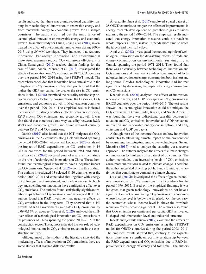
energy use and CO2 emissions. Therefore, transport is respon-sible for both direct emissions from fossil fuels to power trans-port vehicles and indirect emissions through electricity. Roadtransport has a share of 11.9 % in total transport. Road trucksinclude cars, buses, and motorcycles (this group represents60% of total road trucks) and trucks and lorries. Aviation isalso responsible for the carbon emissions from domestic(40%) and international aviation (60%) (Ritchie and Roser2020). Besides, parallel to the increasing demand for modernhighways, infrastructure constructions affect the land surfacedramatically and cause great losses on habitat and biodiversi-ty. The transportation sector is also one of the basic causes ofair pollution-related death and disease such as cancer, asthma,and bronchitis (Rowland et al. 1998: 10). Figure 1 illustratesthe global transport sector’s carbon emission trends over theperiod 2000–2019. World total CO2 emissions steadily in-crease from 5.8 Gt in 2000 to 8.2 Gt in 2019. Comparing withthe shipping and aviation sectors, passenger road vehicles androad freight vehicles contributed more to total CO2 emissions.

IEA (2009a) reported that transport is responsible for onequarter of global energy-related CO2 emissions. However, in2019, the global transport sector energy intensity that is cal-culated by total energy consumption per unit of GDP fell by2.3% (Teter et al. 2020). Besides, the Covid-19 pandemicadversely affected the transportation sector. Until the Covid-19 pandemic started in the early days of 2020, CO2 emissionswere rising around 1% every year in the last 10 years (LeQuéré et al. 2020:647). Due to global lockdown precautions,57% of global oil demand declined. Sharp declines in energydemand in 2020:Q1 led to a 5% fall compared with 2019:Q1in global carbon emissions. Road transport declined between50 and 75%. At the end of March 2020, the global transportactivity fell by 50% of the 2019 level. Indeed, CO2 emissionsdropped more than energy demand since the greatest carbon-incentive fuels had the largest drops in demand during thisperiod. The regions which experienced the earliest impactsof the Covid-19 had the largest CO2 emissions falls. It is alsoexpected that the global lockdown will cause sharp declines in

the global CO2 emissions and will be recorded as 30.6 Gt bythe end of this year. This amount is approximately 8% lowerthan the previous year (IEA 2020a, 2020b). However, oncethe pandemic is over, there may be even more CO2 emissionsin all sectors starting from the transport. Road vehicles such ascars, trucks, buses, and other motor vehicles are responsiblefor ¾ of transport CO2 emissions. Moreover, carbon emis-sions from aviation and shipping are rising which points outthe necessity to have international cooperation and initiatingglobal policies (Teter et al. 2020). IEA (2009b) predicted thatunless there are international cooperation and global mea-sures, worldwide car ownership will be triple to more than 2billion; the trucking sector will be expected to be double, andaviation will increase by fourfold by 2050. These increases inall subsectors of transportation will double the transport ener-gy use that will bring higher rates of CO2 emissions. Indeed,transport energy use and CO2 emissions are estimated to in-crease by 50% by 2030 and more than 80% by 2050 (IEA2009a: 29, 35).

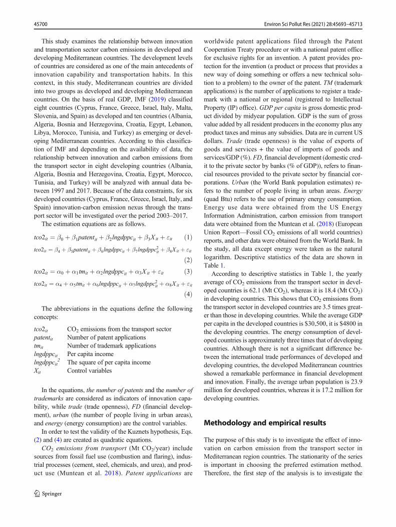
Figure 2 represents the carbon emissions of Mediterraneancountries. We included Israel, Italy, France, Spain, Greece,and Cyprus as developed Mediterranean countries andTurkey, Albania, Bosnia and Herzegovina, Croatia, Algeria,Tunisia, and Morocco as developing Mediterranean countriesin our study. During the 2000–2016 period, carbon emissionsof developed countries were always higher. However, startingfrom 2010, while developingMediterranean countries’ carbonemissions were rising, carbon emissions of developedMediterranean countries started to decline. The decrease incarbon emissions in developed Mediterranean countries canbe due to increasing energy efficiency and innovative technol-ogies in the energy sector.

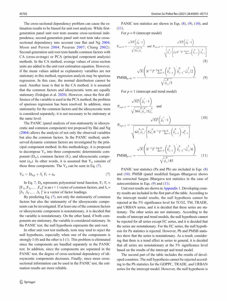
Figure 3 illustrates the carbon emissions of the transportsubsectors in developed and developing Mediterranean coun-tries in 2017. According to Fig. 3, transport combustion byroad is much higher than transport combustion by shippingand aviation both in developed and developingMediterraneancountries.

5.8 5.8 5.9 6.1 6.3 6.5 6.6 6.8 6.8 6.77 7.1 7.2 7.3 7.5 7.7 7.9 8 8.2 8.2

0

1

2

3

4

5

6

7

8

9

World total

transport sector

carbon emissions

Passenger road

vehicles

Road freight

vehicles

Shipping

Aviation

Fig. 1 Global transport sectorcarbon emissions (Gt, 2000–2019). Sources: Teter et al. (2020)and IEA (2019b)

45695Environ Sci Pollut Res (2021) 28:45693–45713

Although historically, there has been a close relationshipbetween economic growth and transportation, there is a trade-off between economic growth, transport increase, and envi-ronmental degradation. The question is whether we can initi-ate sustainable economic growth with less CO2 emissions.Moreover, to avoid the disastrous effect of climate change,global CO2 emissions must be decreased at least by 50%. Toreach this target, transport will have a crucial position. Eventhough there are huge cuts in CO2 in all other sectors, unlesstransport does not reduce CO2 emissions by 2050, it will beimpossible to meet the target (IEA 2009a: 29).

It is a fact that the transport sector is one of the leadingsectors contributing to carbon emissions on a global scale(Chaudhry et al. 2020). Despite the fact that the transportsector causes environmental pollution, it is also one of thepioneer sectors which have the greatest technological devel-opments and innovation that bring energy efficiency and lessfuel consumption. Many studies have pointed out that inno-vation in the transport sector not only provides energy effi-ciency but also increases the service life of vehicles. Besides,the gains in efficiency of energy consumption lead reductionin the per-unit price of energy services. This causes increasesin energy consumption and carbon emissions (the reboundeffect). In their studies, Greening et al. (2000); Herring andRoy (2007); Jin et al. (2018); Erdoğan et al. (2019a); Erdoğan

et al. (2020); Erdoğan et al. (2019b); and Lemoine (2019)pointed out the interrelation between economic growth, tech-nological innovation, and increasing energy consumptionwhich leads rebound effect.

Moreover, the level of development of the countries maybe also crucial in analyzing the contribution of the transportsector to carbon emissions. The findings of the researchesconsidering the development level of the countries in orderto find solutions to combat the increase in carbon emissionson a global scale may be helpful. In this context, the questionsto be answered in order to determine the relationship betweenthe level of development of countries and the magnitude ofcarbon emissions are listed below:

– The lower the economic growth, the less allocation ofsources to be transferred to innovation. Does using lowtechnologies in the transport sector result in high carbonemissions?

– Does higher income per capita in developed countriesaggravate carbon emissions due to the increasing de-mand for energy-saving vehicles? Yet drivers may bemore comfortable driving more if they believe that theirvehicles consume less fuel and produce fewer pollutants.

– How do the demand to own a car and the desire to driveaffect carbon emissions?

100.8 99.2 105.2 110.4 113.2 116.8126.5

139.3 141.7 147 151.8

197.6

218.7 226.3238.1

256.7 264.76

373.5382 386.5 392.9 400.2 400.3 406.6 410.6

392.5378.7 371.5 370.8

342.6 337.3 342.5 346.2357.1

0

50

100

150

200

250

300

350

400

450

2000 2001 2002 2003 2004 2005 2006 2007 2008 2009 2010 2011 2012 2013 2014 2015 2016

Developing

Mediterranean

Countries

Developed

Mediterranean

Countries

Fig. 2 Developed and developing Mediterranean countries carbonemissions from the transportation sector (million tones, 2000–2016).Source: Authors’ own calculations from Ritchie and Roser (2020).

Developing Mediterranean countries: Turkey, Albania, Bosnia andHerzegovina, Croatia, Algeria, Tunisia, and Morocco. DevelopedMediterranean countries: Israel, Italy, France, Spain, Greece, and Cyprus

0

50

100

150

Transport combustion by road Transport combustion by shipping and aviation

Fig. 3 Developed and developingMediterranean countries carbonemissions from transport (Roadand shipping–aviation) (2017,million tones). Source: IEA(2019a)


– Indeed, the level of development difference among thecountries in the Mediterranean region is significant.Does it make a difference in carbon emissions?

In this vein, the aim of this study is to investigate whetherthere is a difference between developed Mediterranean coun-tries and developing Mediterranean countries regarding theimpact of innovation on the transport sector and carbon emis-sions. The Mediterranean basin has been an important andstrategic region, and all countries located in this region havea critical role both in economic and political relations.However, the macroeconomic performances of developedand developing Mediterranean countries demonstrate greatdifferences. The macroeconomic performances of Euro-Mediterranean countries are better than most of the Easternand Southern Mediterranean countries. Thus, their R&D ex-penditures, economic growth rates, GDP per capita, and thelevel of innovation investments are far better than their devel-oping counterparts. Furthermore, energy efficiency technolo-gies, means of the transport sector, and environmental policiesand level of environmental awareness are not homogenous insample countries. Therefore, while developing Mediterraneancountries’ carbon emissions were rising in recent years, car-bon emissions of developed Mediterranean countries startedto decline. This is probably related to increasing energy effi-ciency and innovative technologies in the energy sector.

To provide a precise analysis, we divided the Mediterraneancountries into two groups as developed Mediterranean coun-tries and developing Mediterranean countries. Based on theavailable reliable data, Albania, Algeria, Bosnia andHerzegovina, Croatia, Egypt, Morocco, Tunisia, and Turkeyare selected as the 8 developing countries; and Cyprus,France, Greece, Israel, Italy, and Spain are selected as the 6developed countries. We kindly explain the reasons why wedistinguished the sample countries as developed and develop-ing Mediterranean countries. Since the income per capita indeveloped countries is higher than in developing coun-tries, it is possible for these countries to transfer moreresources to the area of innovation. Transferring moreresources to innovation investments can be helpful to con-trol and reduce environmental degradation. Therefore, in-novation in developed countries is expected to be moreeffective in reducing carbon emissions comparing to de-veloping countries. In order to analyze whether this ex-pectation is correct or not, the countries within the scopeof the study have been classified as developed and devel-oping countries. Due to data constraints, the analysis pe-riod has been determined as 1997–2017 for the develop-ing Mediterranean countries and 2003–2017 for the devel-oped Mediterranean countries. After determining the long-term relationship with the panel co-integration method,we obtained the long-term coefficients with FMOLS andDOLS methods. We applied Pedroni co-integration test. It

allows for panel-specific co-integrating vectors and basedon the stationarity test of error terms with panel and grouptests statistics (v, rho, ADF, and PP).

To the best of our knowledge, there is no other studythat investigates the effects of innovation on the transportsector carbon emissions in the Mediterranean countries.Hence, the contribution of our paper to the related litera-ture is analyzing the relationship between innovation andtransport sector carbon emissions in the developed anddeveloping Mediterranean countries.

The remainder of the paper is organized as follows: Thesecond part is the literature review. The third part introducesthe model; the fourth part explains the data and methodology,the statistical properties of data, and stylized facts; and the lastpart presents the empirical results and policy implications.

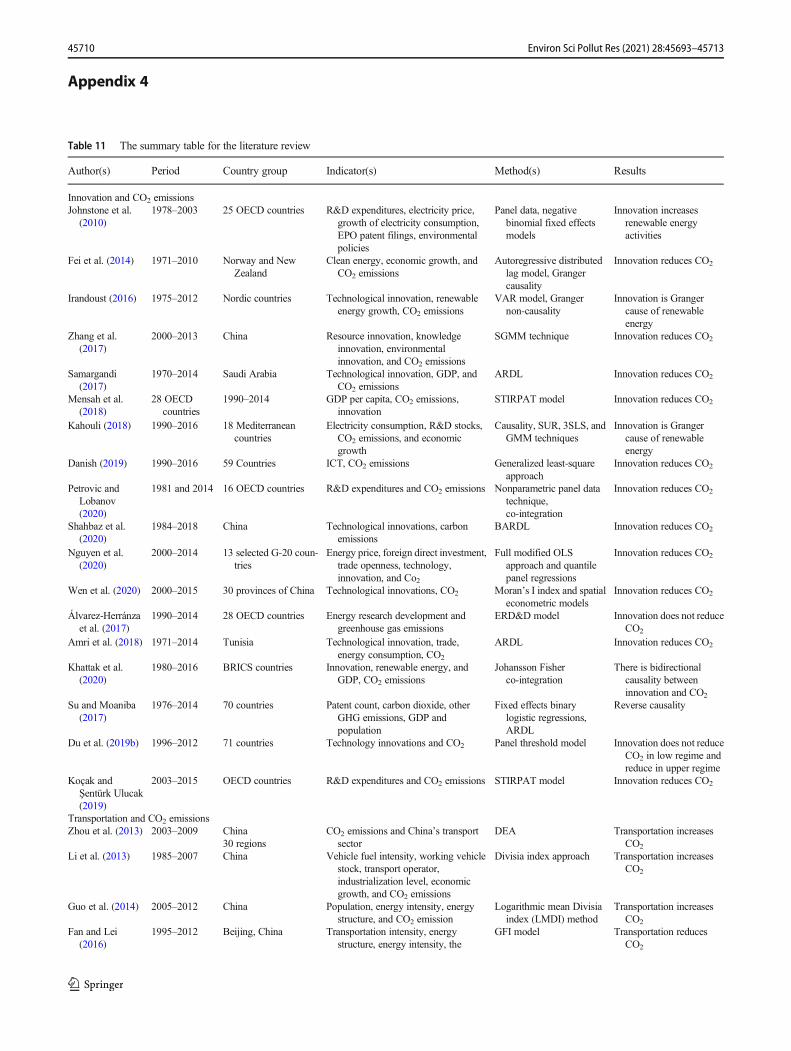
Literature review

The literature review of our study will be analyzed under twoheadlines: The first headline is the relationship between thetransportation sector and CO2 emissions. And the second oneis the relationship between innovation and CO2 emissions.The summary table for the literature review can be seen inAppendix 4.

Innovation and CO2 emissions

Johnstone et al. (2010) examined the effects of environmentalpolicies on technological innovation in the case of renewableenergy on the 25 OECD countries using the panel data duringthe period 1978–2003. The researchers concluded that publicpolicy had a crucial role in determining patent applicationsand the development of new renewable energy technologies.The authors pointed the public expenditures on R&D and theKyoto Protocol that encouraged the patent activities on windand solar power as the significant effects on increasing inno-vation activities.

Fei et al. (2014) investigated the energy–growth nexus bytaking the effects of clean energy, CO2 emissions, and tech-nological innovation into account in Norway and NewZealand during the period 1971–2010. The authors indicatedthat there was a long-term equilibrium between clean energy,economic growth, and CO2 emissions. They also showed thatwhile clean energy alleviates the CO2 emissions, it also bringsextra cost on the economic growth of both countries. Whiletechnological innovation implies advancements in energyefficiency, New Zealand does not intend to applytechnological innovation in clean energy production.Irandoust (2016) analyzed the relationship between renewableenergy consumption, technological innovation, CO2 emis-sions, and economic growth in the Nordic countries(Denmark, Finland, Norway, and Sweden). The empirical


results indicated that there was a unidirectional causality run-ning from technological innovation to renewable energy andfrom renewable energy to economic growth for all samplecountries. The authors pointed out the importance oftechnological innovation on renewable energy and economicgrowth. In another study for China, Zhang et al. (2017) inves-tigated the effect of environmental innovations during 2000–2013 using SGMM technique. They indicated that resourceinnovation, knowledge innovation, and environmentalinnovation measures reduce CO2 emissions effectively inChina. Samargandi (2017) reached similar findings for thecase of Saudi Arabia. Mensah et al. (2018) investigated theeffects of innovation on CO2 emission in 28 OECD countriesover the period 1990–2014 using the STIRPAT model. Theresearchers concluded that innovation has a crucial role in themitigation of CO2 emissions. They also pointed out that thehigher the GDP per capita, the greater the rise in CO2 emis-sions. Kahouli (2018) examined the causality relationship be-tween energy electricity consumption, R&D stocks, CO2

emissions, and economic growth in Mediterranean countriesover the period 1990–2016. The empirical results indicatedthe existence of strong feedback effects between electricity,R&D stocks, CO2 emissions, and economic growth. It wasalso found that there was a one-way causality between R&Dstocks and economic growth, and a unidirectional causalitybetween R&D and CO2 emissions.

Danish (2019) also found that the ICT mitigates the CO2

emissions in the 59 countries along Belt and Road spanningthe period 1990–2016. Petrovic and Lobanov (2020) analyzedthe impact of R&D expenditures on CO2 emissions in 16OECD countries for the period between 1981 and 2014.Shahbaz et al. (2020) revealed parallel results in their studyon the role of technological innovations in China. The authorsfound that technological innovations have a negative impacton CO2 emissions. Nguyen et al. (2020) confirm this finding.The authors investigated 13 selected G-20 countries over theperiod 2000–2014 and concluded that together with energyprice, foreign direct investment, and trade openness, technol-ogy and spending on innovation have a mitigating effect overCO2 emissions. The authors found statistically significant re-lationships between CO2 emissions, innovation, and ICT. Theauthors found that R&D investment has negative effects onCO2 emissions in the long term. They showed that a 1%growth of R&D investments mitigates CO2 emissions by0.09–0.15% on average. Wen et al. (2020) analyzed the spill-over effects of technological innovation on CO2 emissions in30 provinces of China spanning the period 2000–2015 in theconstruction sector. The authors indicated the key role of tech-nological innovation in CO2 emission reduction in the con-struction industry.

Although most of the studies in the literature indicated themoderating effects of innovation on CO2 emissions, there aresome studies that reached different results:

Álvarez-Herránza et al. (2017) employed a panel dataset of28 OECD countries to analyze the effects of improvements inenergy research development on greenhouse gas emissionsspanning the period 1990––2014. The empirical results indi-cated that energy innovation measures could not reach itswhole impacts at once, instead, it needs more time to reachthe targets and their full effect.

Amri et al. (2018) investigated the moderating role of tech-nological innovation on the devastating effects of trade andenergy consumption on environmental sustainability inTunisia spanning the period 1971–2014. They found thatthere was no causality between technological innovation andCO2 emissions and there was a unidirectional impact of tech-nological innovation on energy consumption both in short andlong terms. Besides, technological innovation had indirectsignificance by decreasing the impact of energy consumptionon CO2 emissions.

Khattak et al. (2020) analyzed the effects of innovation,renewable energy, and GDP per capita on CO2 emissions inBRICS countries over the period 1980–2016. The test resultsshowed that technological innovation could not mitigate theCO2 emissions in China, India, Russia, and South Africa. Itwas found that there was bidirectional causality between in-novation and CO2 emissions; innovation and GDP per capita;innovation and renewable energy consumption; and CO2

emissions and GDP per capita.Although most of the literature focuses on how innovation

contributes to alleviating climate impact on the environmentby examining the mitigating innovative technologies, Su andMoaniba (2017) tried to analyze the causality via a reverseapproach. The authors analyzed the effects of climate changeson innovation technologies on a dataset of 70 countries. Theauthors concluded that increasing levels of CO2 emissionscause more innovations related to climate change. Therefore,the author suggested diverting public funds to innovative ac-tivities that contribute to combating climate change.

Du et al. (2019b) investigated the effects of green technol-ogy innovations on CO2 emissions in 71 countries for theperiod 1996–2012. Based on the empirical findings, it wasindicated that green technology innovations do not have asignificant impact on mitigating CO2 emissions in economieswhose income level is below the threshold. On the contrary,the economies whose income level is above the thresholdreduction effects became significant. The authors also foundthat CO2 emission per capita and per capita GDP is invertedU-shaped and urbanization level and industrial structure.

Koçak and Şentürk Ulucak (2019) examined the effects ofR&D expenditures on CO2 emissions using the STIRPATmodel for OECD countries during the period 2003–2015.The empirical results showed that, contrary to the expecta-tions, there was a significant positive relationship betweenthe R&D expenditures and CO2 emissions due to R&D im-provements in energy efficiency and fossil fuel. The authors


also found that the power and storage R&D expenditures havea mitigating effect on CO2 emissions.

Transportation and CO2 emissions

Zhou et al. (2013) examined the CO2 emissions performanceof China’s transport sector over the period 2003–2009. Theempirical results indicated that the number of environmentallyefficient regions decreased in the given period. The authorsalso found that the Eastern region of the country had the bestresults in adjusting CO2 emissions as transport infrastructurefacilities are better in this region. Hence, they underlined theimportance of the development of transport infrastructuretechnologies in the abatement of CO2 emissions.

Li et al. (2013) explored the effects of factors such as ve-hicle fuel intensity, working vehicle stock per freight transportoperator, industrialization level, and economic growth on theCO2 emissions from road freight transportation in China overthe period 1985–2007. The test results showed that while eco-nomic growth is the most important factor in increasing CO2

emissions, the ton-kilometer per value added of industry andthe market concentration level significantly decrease CO2

emissions.Guo et al. (2014) analyzed the contributions of population,

energy intensity, energy structure, and economic activities toCO2 emission increments in the transport sector spanning theperiod 2005–2012 in different provinces and regions of China.The authors concluded that the Eastern region of China hadthe highest CO2 emissions and per capita CO2 emissions butthe lowest CO2 emissions intensity in its transport sector,whereas the Western side had the highest CO2 emission inten-sity and the fastest emission increasing trend in its transportsector. They also pointed out that there has been a great in-crease in CO2 emissions in the transport sector in parallel toeconomic activities.

Fan and Lei (2016) explored the impact of transportationintensity, energy structure, energy intensity, the output valueof per unit traffic turnover, population, and economic growthon CO2 emissions in the transportation sector over the period1995–2012 in Beijing, China. The authors found that econom-ic growth, energy intensity, and size of the population are theprimary reasons for transportation carbon emissions. Theyalso found that transportation intensity and energy structureare the negative drivers of CO2 emissions in the transportationsector.

Wang and He (2017) investigated the CO2 marginal miti-gation costs of the regional transportation sector, CO2 emis-sions efficiency, economic efficiency, and productivity inChina from 2007 to 2012. The authors found that CO2 emis-sions efficiency and marginal mitigation cost of CO2 emis-sions are negatively correlated. Hence, improving CO2 emis-sions efficiency leads to a reduction in CO2 marginal mitiga-tion costs.

Zhu and Du (2019) analyzed the driving factors of CO2

emissions of road transportation in Australia, Canada, China,India, Russia, and the USA for the period of 1990–2016. Theempirical results indicated that carbon emissions of road trans-portation had a dramatic increase since 1990. Besides, boththe economic output and the increasing population had posi-tive effects on CO2 emissions of the road transportation sector.

Du et al. (2019a) analyzed the relationship between thetransportation sector and the Chinese economy from 2002 to2012. The authors searched the effects of all means of trans-portation, i.e., the rail, road, water, and air on the generation ofCO2 emissions. The empirical findings indicated that the roadsubsector increased CO2 emissions whereas the rail subsectorresulted in mitigation in CO2 emissions due to technologicaladvances.

Khan et al. (2020) investigated the sectorial effects on CO2

emission in Pakistan over the period 1991–2017. The re-searcher revealed that while the agriculture and services sec-tors have a negative effect on CO2 emissions, the construction,manufacturing, and transportation sectors contribute to theCO2 emissions. They also pointed out the importance of tech-nological innovations for the CO2 emissions reductionstrategies.

Georgatzi et al. (2020) examined the determinants of CO2

emissions due to the transport sector for 12 European coun-tries during the period 1994–2014. Based on the test results, itwas concluded that infrastructure investments by the transportsector do not have a significant effect on CO2 emissions; andalso, there was a bidirectional relationship between environ-mental policy stringency and CO2 emissions.

Although in most of the studies researchers found similarresults that point to the positive relationship between the trans-port sector and CO2 emissions, some papers indicated that theresults may vary. In their study on the impact of publictransportation on CO2 emissions for Chinese provinces,Jiang et al. (2018) concluded that although the results wereheterogeneous, the findings support inverted U-shaped nexusbetween public transportation and CO2 emissions for prov-inces whose CO2 emission levels are different. Hence, if thepublic transportation level exceeds a threshold value, the rela-tionship between the two variables may turn from positive tonegative.

Data

There are many factors affecting CO2 emissions such as thesize of population, urbanization, economic growth, FDI, fi-nancial development, trade, and energy intensity (Phamet al. 2020; Nasir et al. 2019). Innovation is also very effectiveon CO2 emissions. Thus, analyzing the effects of innovationon a sectorial basis may be useful for developing specificpolicies.


This study examines the relationship between innovationand transportation sector carbon emissions in developed anddeveloping Mediterranean countries. The development levelsof countries are considered as one of the main antecedents ofinnovation capability and transportation habits. In thiscontext, in this study, Mediterranean countries are dividedinto two groups as developed and developing Mediterraneancountries. On the basis of real GDP, IMF (2019) classifiedeight countries (Cyprus, France, Greece, Israel, Italy, Malta,Slovenia, and Spain) as developed and ten countries (Albania,Algeria, Bosnia and Herzegovina, Croatia, Egypt, Lebanon,Libya, Morocco, Tunisia, and Turkey) as emerging or devel-oping Mediterranean countries. According to this classifica-tion of IMF and depending on the availability of data, therelationship between innovation and carbon emissions fromthe transport sector in eight developing countries (Albania,Algeria, Bosnia and Herzegovina, Croatia, Egypt, Morocco,Tunisia, and Turkey) will be analyzed with annual data be-tween 1997 and 2017. Because of the data constraints, for sixdeveloped countries (Cyprus, France, Greece, Israel, Italy, andSpain) innovation-carbon emission nexus through the trans-port sector will be investigated over the period 2003–2017.

The estimation equations are as follows.

tco2it ¼ β0 þ β1patentit þ β2lngdppcit þ β3X it þ εit ð1Þtco2it ¼ β4 þ β5patentit þ β6lngdppcit þ β7lngdppc

2it þ β8X it þ εit

ð2Þtco2it ¼ α0 þ α1tmit þ α2lngdppcit þ α3X it þ εit ð3Þtco2it ¼ α4 þ α5tmit þ α6lngdppcit þ α7lngdppc2it þ α8X it þ εit

ð4Þ

The abbreviations in the equations define the followingconcepts:

tco2it CO2 emissions from the transport sectorpatentit Number of patent applicationstmit Number of trademark applicationslngdppcit Per capita incomelngdppcit

2 The square of per capita incomeXit Control variables

In the equations, the number of patents and the number oftrademarks are considered as indicators of innovation capa-bility, while trade (trade openness), FD (financial develop-ment), urban (the number of people living in urban areas),and energy (energy consumption) are the control variables.

In order to test the validity of the Kuznets hypothesis, Eqs.(2) and (4) are created as quadratic equations.

CO2 emissions from transport (Mt CO2/year) includesources from fossil fuel use (combustion and flaring), indus-trial processes (cement, steel, chemicals, and urea), and prod-uct use (Muntean et al. 2018). Patent applications are

worldwide patent applications filed through the PatentCooperation Treaty procedure or with a national patent officefor exclusive rights for an invention. A patent provides pro-tection for the invention (a product or process that provides anew way of doing something or offers a new technical solu-tion to a problem) to the owner of the patent. TM (trademarkapplications) is the number of applications to register a trade-mark with a national or regional (registered to IntellectualProperty (IP) office). GDP per capita is gross domestic prod-uct divided by midyear population. GDP is the sum of grossvalue added by all resident producers in the economy plus anyproduct taxes and minus any subsidies. Data are in current USdollars. Trade (trade openness) is the value of exports ofgoods and services + the value of imports of goods andservices/GDP (%).FD, financial development (domestic cred-it to the private sector by banks (% of GDP)), refers to finan-cial resources provided to the private sector by financial cor-porations. Urban (the World Bank population estimates) re-fers to the number of people living in urban areas. Energy(quad Btu) refers to the use of primary energy consumption.Energy use data were obtained from the US EnergyInformation Administration, carbon emission from transportdata were obtained from the Muntean et al. (2018) (EuropeanUnion Report—Fossil CO2 emissions of all world countries)reports, and other data were obtained from theWorld Bank. Inthe study, all data except energy were taken as the naturallogarithm. Descriptive statistics of the data are shown inTable 1.

According to descriptive statistics in Table 1, the yearlyaverage of CO2 emissions from the transport sector in devel-oped countries is 62.1 (Mt CO2), whereas it is 18.4 (Mt CO2)in developing countries. This shows that CO2 emissions fromthe transport sector in developed countries are 3.5 times great-er than those in developing countries. While the average GDPper capita in the developed countries is $30,500, it is $4800 inthe developing countries. The energy consumption of devel-oped countries is approximately three times that of developingcountries. Although there is not a significant difference be-tween the international trade performances of developed anddeveloping countries, the developed Mediterranean countriesshowed a remarkable performance in financial developmentand innovation. Finally, the average urban population is 23.9million for developed countries, whereas it is 17.2 million fordeveloping countries.

Methodology and empirical results

The purpose of this study is to investigate the effect of inno-vation on carbon emission from the transport sector inMediterranean region countries. The stationarity of the seriesis important in choosing the preferred estimation method.Therefore, the first step of the analysis is to investigate the


stationarity of the series. Another important factor affect-ing the estimation results in panel data analysis is cross-sectional dependency. O’Connell (1998) showed thatcross-sectional dependency increases the possibility ofrejecting the null hypothesis. Panel unit root tests can bedivided into two: (1) first-generation unit root tests as-suming cross-sectional independence of series and (2)second-generation unit root tests assuming cross-sectional dependence of series. In order to choose theappropriate estimation method, it is necessary to investi-gate the cross-sectional dependency of the series.

The Pesaran (2004) CD test and Pesaran and Yamagata(2008) LMadj (bias-adjusted cross-sectional dependenceLagrange multiplier) test were used to test the presence ofcross-sectional dependence.

CD test statistics are calculated as follows:

CD ¼ffiffiffiffiffiffiffiffiffiffiffiffiffiffiffiffiffiffiffiffiffiffiffiffiffiffiffiffiffiffiffiffiffiffiffiffiffiffiffiffiffiffiffiffiffiffiffiffiffiffiffi

2TN N−1ð Þ ∑N−1

i¼1 ∑Nj¼iþ1bρij� �s

⟹N 0; 1ð Þ ð5Þ

LMadj test statistics are calculated as follows:

LMadj ¼ffiffiffiffiffiffiffiffiffiffiffiffiffiffiffiffiffi

2

N N−1ð Þ

s∑N−1

i¼1 ∑Nj¼iþ1Tbρij T−kð Þbρ2ij−μTijffiffiffiffiffiffiffi

υ2Tijq ð6Þ

Hypotheses of CD test:H0: No cross-sectional dependenceH1: Has the cross-sectional dependence

Table 2 shows the results of the cross-sectional dependencyof the series.

As shown in Table 2, according to the CD test results, thenull hypothesis is rejected at the 10% significance level.The basic hypothesis suggests that there is no cross-sectional dependency for all variables except theGDPPC series. Hence, it is decided that the cross-

sectional dependency problem exists. For the GDPPC se-ries, it is seen that the basic hypothesis cannot be stronglyrejected. On the other hand, according to the LMajd testresult for the GDPPC series, the basic hypothesis suggest-ing that there is no cross-sectional dependency is rejected,and it is decided that the cross-sectional dependency prob-lem exists. According to the results of the LMajd test, it isdecided that the cross-sectional dependency problem ex-ists for all series except for TM, TRADE, and FD series.

According to CD test results at a 10% significance level fordeveloped countries, it is decided that the cross-sectional de-pendency problem exists for all variables except GDPPC,URBAN, and FD series. For these three variables, LMajd teststatistics show that the cross-sectional dependency problemexists. According to the LMajd test result, it is decided thatthe cross-sectional dependency problem exists for all seriesexcept TCO2, PAT, and TM series. However, the basic hy-pothesis cannot be strongly rejected within these series; thetest statistics almost exceed the 10% level. As a result, it wasdecided that the cross-sectional dependency problem existsfor all series in the analysis.

PANIC test

In our study, the PANIC (panel analysis of non-stationarity inidiosyncratic and common component) test proposed by Baiand Ng (2004) will be used. In this method, if the mean valuesadded as explanatory variables are not stationary, regressionanalysis may be spurious regression. In this case, normal dis-tribution will not be used. Also, in the CA method, the com-mon factors and idiosyncratic term are assumed to be equallystationary (Erdoğan et al. 2020). However, since the first dif-ference of the variable is used in the PCAmethod, the problemof spurious regression disappears. Besides, since stationarityfor the common factors and idiosyncratic term is consideredseparately, it is not necessary for them to be stationary at thesame level.

Table 1 Descriptive statistics

Variables

TCO2 GDPPC EC TM PAT FD TRADE URBAN

Developed countries

Min. 1.7 18116.5 0.1 1569.0 3.0 57.17 45.6 681117.0

Max. 133.1 45334.1 11.5 94917.0 17290.0 253.2 133.0 53612472.0

St. err. 51.0 6723.7 4.0 30308.6 5778.6 52.0 22.5 19228178.0

Average 62.1 30512.1 4.5 33640.9 6192.6 115.0 68.4 23898068.4

Developing countries

Min. 1.3 1033.2 0.1 2224.0 4.0 4.9 30.2 1279853.0

Max. 85.9 16357.2 6.4 119304.0 8555.0 95.5 121.8 60537696.0

St. err. 19.0 3600.9 1.5 25449.5 1309.2 22.6 19.4 16860375.1

Average 18.4 4800.9 1.4 15436.7 1010.2 45.1 72.1 17261533.7


The cross-sectional dependency problem can cause the es-timation results to be biased for unit root analysis. While first-generation panel unit root tests assume cross-sectional inde-pendence, second-generation panel unit root tests take cross-sectional dependency into account (see Bai and Ng 2004;Moon and Perron 2004; Pesaran 2007; Chang 2002).Second-generation unit root tests handle common factors withCA (cross-average) or PCA (principal component analysis)methods. In the CA method, average values of cross-sectionunits are added to the unit root estimation equation. However,if the mean values added as explanatory variables are notstationary in this method, regression analysis may be spuriousregression. In this case, the normal distribution cannot beused. Another issue is that in the CA method, it is assumedthat the common factors and idiosyncratic term are equallystationary (Erdoğan et al. 2020). However, since the first dif-ference of the variable is used in the PCAmethod, the problemof spurious regression has been resolved. In addition, sincestationarity for the common factors and the idiosyncratic termis considered separately, it is not necessary to be stationary atthe same level.

The PANIC (panel analysis of non-stationarity in idiosyn-cratic and common component) test proposed by Bai and Ng(2004) allows the analysis of not only the observed variablesbut also the common factors. In the PANIC method, unob-served dynamic common factors are investigated by the prin-cipal component method. In this methodology, it is proposedto decompose Yit into three components: deterministic com-ponent (Dit,), common factors (Ft), and idiosyncratic compo-nent (eit). In other words, it is assumed that Yit consists ofthese three components. The Yit can be seen in Eq. (7).

Yit ¼ Dit;p þ λ0i Ft þ eit ð7Þ

In Eq. 7, Dit represents polynomial trend function, Ft: Ft =[F1t ,F2t ,… ,Frt]′ is an r × 1 vector of common factors, and λi =[λ1 ,λ2 ,… ,λr ]′ is a vector of factor loadings.

By predicting Eq. (7), not only the stationarity of commonfactors but also the stationarity of the idiosyncratic compo-nents can be investigated. If at least one of the common factorsor idiosyncratic component is nonstationary, it is decided thatthe variable is nonstationary. On the other hand, if both com-ponents are stationary, the variable is considered stationary. Inthe PANIC test, the null hypothesis represents the unit root.

In other unit root test methods, tests may tend to reject thenull hypothesis, especially when one of the components isstrongly I (0) and the other is I (1). This problem is eliminatedsince the components are handled separately in the PANICtest. In addition, since the components are separated in thePANIC test, the degree of cross-sectional dependency of idi-osyncratic components decreases. Finally, since more cross-sectional information can be used in the PANIC test, the esti-mation results are more reliable.

PANIC test statistics are shown in Eqs. (8), (9), (10), and(11).

For p = 0 (intercept model)

Pa;p¼0 ¼ffiffiffiffiffiffiffiNT

p bρþ0 −1� �ffiffiffiffiffiffiffiffiffiffiffiffiffi2bϕ4

εbω4

ε

q and Pb;p¼0 ¼ffiffiffiffiffiffiffiNT

p bρþ0 −1� �ffiffiffiffiffiffiffiffiffiffiffiffiffiffiffiffiffiffiffiffiffiffiffiffiffiffiffiffiffiffiffiffiffiffiffiffiffiffiffiffiffiffiffiffiffiffiffiffiffiffiffiffiffiffiffiffiffiffiffiffiffiffiffiffiffibϕ4

ε= bω3N−1T−2∑Ni¼1 be0i;−1� �’be0i;−1

" #vuutð8Þ

PMSBp¼0 ¼

ffiffiffiffiN

pN−1T−2∑N

i¼1 be0i;−1� �’be0i;−1−bω2

ε=2

!ffiffiffiffiffiffiffiffiffiffibϕ4

ε=3

q ð9Þ

For p = 1 (intercept and trend model)

Pa;p¼1 ¼

ffiffiffiffiffiffiffiNT

p bρþ1 −1� �ffiffiffiffiffiffiffiffiffiffiffiffiffiffiffiffiffi36bσ4

εbϕ4

ε=

q5bω8

ε

and

Pb;p¼1 ¼ffiffiffiffiffiffiffiNT

p bρþ1 −1� �ffiffiffiffiffiffiffiffiffiffiffiffiffiffiffiffiffiffiffiffiffiffiffiffiffiffiffiffiffiffiffiffiffiffiffiffiffiffiffiffiffiffiffiffiffiffiffiffiffiffiffiffiffiffiffiffiffiffiffiffiffiffiffiffiffiffiffiffiffiffiffiffiffiffi6bσ4

εbϕ4

ε= 5bω6

εN−1T−2∑N

i¼1 be0i;−1� �’

e0i;−1

" #vuutð10Þ

PMSBp¼1 ¼

ffiffiffiffiN

pN−1T−2∑N

i¼1 be0i;−1� �’be0i;−1−bω2

ε=6

!ffiffiffiffiffiffiffiffiffiffiffiffibϕ4

ε=45

q ð11Þ

PANIC test statistics (Pa and Pb) are included in Eqs. (8)and (10). PMSB (panel modified Sargan–Bhargava) showsthe corrected Sargan–Bhargava test statistics in the case ofautocorrelation in Eqs. (9) and (11).

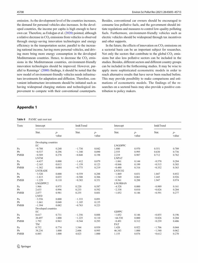
Unit root results are shown inAppendix 1. Developing coun-try results are included in the first part of the table. According tothe intercept model results, the null hypothesis cannot berejected at the 5% significance level for TCO2, TM, TRADE,and URBAN series, and it is decided that these series are sta-tionary. The other series are not stationary. According to theresults of intercept and trend models, the null hypothesis cannotbe rejected for all series except EC series, and it is decided thatthe series are nonstationary. For the EC series, the null hypoth-esis for Pa statistics is rejected. However, Pb and PMSB statis-tics show that the series is nonstationary. As a result, consider-ing that there is a trend effect in series in general, it is decidedthat all series are nonstationary at the 5% significance levelbased on the results of the intercept and trend model.

The second part of the table includes the results of devel-oped countries. The null hypothesis cannot be rejected accord-ing to the Pb statistics for the GDPPC, TRADE, and URBANseries for the intercept model. However, the null hypothesis is


rejected for Pa and PMSB test statistics. According to Pa andPb statistics for the TCO2 series, the null hypothesis cannot berejected, but the null hypothesis is rejected for the PMSB teststatistics. The results of the intercept and trend model indicat-ed that the null hypothesis cannot be rejected for all seriesexcept the PAT series, and it is decided that the series arenonstationary. For the PAT series, the null hypothesis cannotbe strongly rejected. In addition, Pb and PMSB statistics showthat the series is nonstationary. As a result, since we considerthat there is a trend effect in series as a general similar to thedeveloping countries, it is decided that all series are nonsta-tionary at the 5% significance level based on the results offixed and trended model.

After investigating the degree of integration of the series, itis necessary to determine whether the estimation equationsprovide the assumption of cross-sectional independence andhomogeneity in order to select the appropriate co-integrationmethod and estimators. As explained before, for cross-sectional dependence, the Pesaran (2004) CD test andPesaran et.al. (2008) LMadj (bias-adjusted cross-sectional de-pendence Lagrange multiplier) test are used. In order to inves-tigate the homogeneity assumption, Pesaran and Yamagata(2008) tests that are widely used in the literature are preferred.

Pesaran and Yamagata (2008: 54-55) proposed the delta(Δ) test by developing the Swamy (1970) test to investigatehomogeneity. Test statistics and hypotheses of the Delta testare as follows:

bΔ ¼ffiffiffiffiN

p N−1bS−kffiffiffiffiffi2k

p !

for bigger sample ð12Þ

eΔadj ¼ffiffiffiffiN

p N−1eS−kffiffiffiffiffi2k

p !

for smaller sample ð13Þ

H0: βi = β slope coefficients are homogeneousH1: β ≠ βj, slope coefficients are not homogeneous

Table 3 shows the test results of the equations consideredwithin the scope of the analysis for homogeneity and cross-sectional dependency.

According to the results in Table 3, the null hypothesisthat the slope coefficient for the homogeneity test results ishomogeneous is rejected, and it is decided that all estima-tion equations are heterogeneous. On the other hand, ac-cording to both CD test (Pesaran 2004) and LMadj test(Pesaran et al., 2008), the basic hypothesis that suggeststhat there is no cross-sectional dependency cannot berejected for all equations, and it is decided that the problemof cross-sectional dependency does not exist in the equa-tions. Therefore, it is necessary to use heterogeneousmodels in data analysis. Also, taking the cross-sectionaldependency into consideration is important. Nevertheless,since there is no cross-sectional-dependency for estimatedequations in our samples, Pedroni and Durbin–Hausmanpanel co-integration tests are preferred to investigate theco-integration relations between the series.

Pedroni panel co-integration test

The Pedroni co-integration test which allows for panel-specific co-integrating vectors is based on the stationarity testof error terms with panel and group tests statistics (v, rho,ADF, and PP). The Pedroni test also allows individual slopecoefficients and trend coefficients between cross sections. Itdeveloped seven test statistics consisting of within groups andbetween groups tests (within groups tests assume that the ARparameter is the same and the between groups tests assumethat AR parameter varies). These test statistics consist of 4within dimension (panel co-integration statistics) and 3 be-tween dimension (group-mean statistics) tests. In the Pedronico-integration test, the basic hypothesis suggests that there isno co-integration relationship is tested. The alternative hy-pothesis states that at least one unit is cointegrated. Group-mean statistics also provides additional information on

Table 2 Cross-sectionaldependence tests Variables

TCO2 EC GDPPC PAT TM TRADE URBAN FD


CD stat. −2.485 −1.886 −1.163 −2.364 −1.425 −2.138 −1.304 −2.092Prob. 0.006 0.030 0.122 0.009 0.077 0.016 0.096 0.018

LMadj stat. 3.647 3.206 4.066 12.741 −0.124 0.294 27.471 0.550

Prob. 0.000 0.001 0.000 0.000 0.549 0.384 0.000 0.291

Developed countries

CD stat. −1.656 −1.444 1.044 −1.636 −1.367 −1.834 −1.026 −0.630Prob. 0.049 0.074 0.148 0.051 0.086 0.033 0.152 0.264

LMadj stat. 0.931 1.497 3.142 1.243 0.629 1.823 1.354 5.511

Prob. 0.176 0.067 0.001 0.107 0.265 0.034 0.088 0.000


heterogeneity between units. The seven predicted test statisticsfor co-integration analysis are shown as follows:

Panel v−statistic : T 2N 3=2ZbvN ;T≡T 2N 3=2 ∑N

i¼1∑Tt¼1bL−211ibe2i;t−1� �−1

ð14Þ

Panel ρ−statistic : TffiffiffiffiN

pZbpN ;T−1

≡TffiffiffiffiN

p∑N

i¼1∑Tt¼1bL−211ibe2i;t−1� �−1

∑Ni¼1∑

Tt¼1bL−211i be2i;t−1Δbei;t−bλi

� � ð15Þ

Panel t−statistic : ZtN ;T≡ eσ2∑N

i¼1∑Tt¼1bL−211ibe2i;t−1� �−1=2

∑Ni¼1∑

Tt¼1bL−211i be2i;t−1Δbei;t−bλi

� �nonparametricð Þ

ð16Þ

Panel t−statistic : Z*tN ;T≡ s*2N ;T∑

Ni¼1∑

Tt¼1bL−211ibe*2i;t−1� �−1=2

∑Ni¼1∑

Tt¼1bL−211i be*2i;t−1Δbe*i;t� �

parametricð Þð17Þ

Group ρ−statistic : TN−1=2eZbρN ;T−1≡TN−1=2∑N

i¼1 ∑Tt¼1be2i;t−1� �−1

∑Tt¼1 bei;t−1Δbei;t−bλi

� � ð18Þ

Group t−statistic : N−1=2eZtN ;T≡N−1=2∑Ni¼1 bσ2i ∑T

t¼1be2i;t−1� �−1=2

∑Tt¼1 bei;t−1Δbei;t−bλi

� �nonparametricð Þ

ð19Þ

Group t−statistic : N−1=2eZ*

tN ;T≡N−1=2∑N

i¼1 ∑Tt¼1bs*2i be2i;t−1� �−1=2

∑Tt¼1be*2i;t−1Δbe*i;t parametricð Þ

ð20Þ

In Pedroni (2004), panel t- and group t-statistics are obtain-ed from the regressions shown as follows:

bei;t ¼ bγibei;t−1 þ bμi;t; ð21Þ

bei;t ¼ bγibei;t−1 þ ∑Kik¼1bγi;kΔbei;t−k þ bμ*

i;t ð22Þ

Panel ρ- and panel t-statistics are estimated by the long-term variance of ηit by the following regression:

ΔY it ¼ αi þ δit þ βiΔX it þ ηit ð23Þ

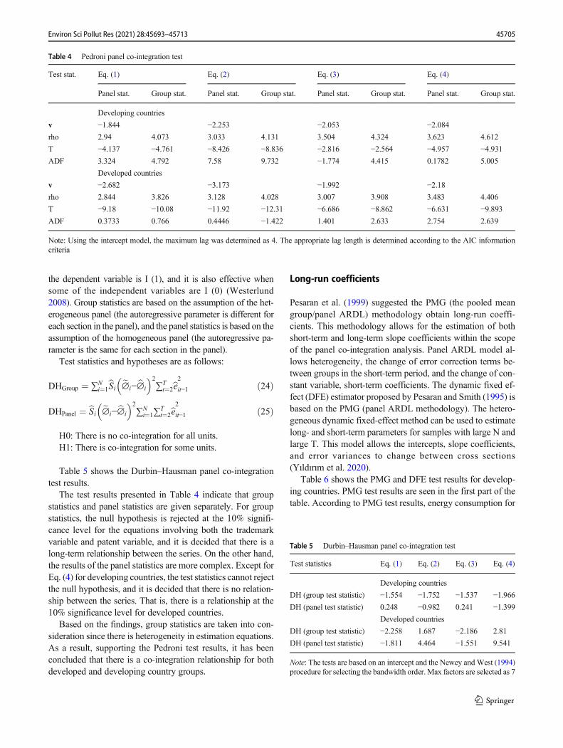
Pedroni panel co-integration test results are shown inTable 4.

According to Table 4, the first part illustrates the test resultsfor developing countries for both Eqs. (2) and (4) with trade-mark variables and Eqs. (1)–(3) with the patent variable. In thefirst part, according to all test statistics, the null hypothesissuggesting that there is no co-integration relationship betweenthe series is rejected, and it is decided that a co-integrationrelationship exists. On the other hand, according to the resultsregarding the developed countries in the second part, the nullhypothesis is rejected according to the other test statistics ex-cept for the ADF test statistics for Eqs. (1), (2), and (3), and itis decided that a co-integration relationship exists. As an al-ternative to the Pedroni test, the Durbin–Hausman test waspreferred since it presents panel and group statisticsseparately.

Durbin–Hausman panel co-integration test

The Durbin–Hausman test, developed by Westerlund (2008),takes the cross-sectional dependency into account and pre-sents both panel and group statistics. This test is effective if

Table 3 Homogeneity and cross-sectional dependency tests for equations

Eq. (1) Eq. (2) Eq. (3) Eq. (4)

Homogeneity and cross-sectional dependency tests Stat. Prob. Stat. Prob. Stat. Prob. Stat. Prob.

Developed countriesbΔ 3.652 0.000 2.774 0.003 3.798 0.000 2.886 0.002eΔadj 5.164 0.000 4.195 0.000 5.372 0.000 4.363 0.000

CSD

CD −0.078 0.469 0.289 0.386 0.218 0.414 0.080 0.468

LMadj 0.911 0.181 0.179 0.429 0.400 0.344 0.065 0.474

Developing countriesbΔ 4.243 0.000 3.382 0.000 4.420 0.000 3.709 0.000eΔadj 5.478 0.000 4.561 0.000 5.706 0.000 5.002 0.000

CSD

CD −1.102 0.135 −0.562 0.287 −0.718 0.236 −0.395 0.347

LMadj −0.992 0.839 0.464 0.321 −1.463 0.928 −1.206 0.886


the dependent variable is I (1), and it is also effective whensome of the independent variables are I (0) (Westerlund2008). Group statistics are based on the assumption of the het-erogeneous panel (the autoregressive parameter is different foreach section in the panel), and the panel statistics is based on theassumption of the homogeneous panel (the autoregressive pa-rameter is the same for each section in the panel).

Test statistics and hypotheses are as follows:

DHGroup ¼ ∑Ni¼1bSi e∅i−b∅i

� �2∑T

t¼2be2it−1 ð24Þ

DHPanel ¼ bSi e∅i−b∅i

� �2∑N

i¼1∑Tt¼2be2it−1 ð25Þ

H0: There is no co-integration for all units.H1: There is co-integration for some units.

Table 5 shows the Durbin–Hausman panel co-integrationtest results.

The test results presented in Table 4 indicate that groupstatistics and panel statistics are given separately. For groupstatistics, the null hypothesis is rejected at the 10% signifi-cance level for the equations involving both the trademarkvariable and patent variable, and it is decided that there is along-term relationship between the series. On the other hand,the results of the panel statistics are more complex. Except forEq. (4) for developing countries, the test statistics cannot rejectthe null hypothesis, and it is decided that there is no relation-ship between the series. That is, there is a relationship at the10% significance level for developed countries.

Based on the findings, group statistics are taken into con-sideration since there is heterogeneity in estimation equations.As a result, supporting the Pedroni test results, it has beenconcluded that there is a co-integration relationship for bothdeveloped and developing country groups.

Long-run coefficients

Pesaran et al. (1999) suggested the PMG (the pooled meangroup/panel ARDL) methodology obtain long-run coeffi-cients. This methodology allows for the estimation of bothshort-term and long-term slope coefficients within the scopeof the panel co-integration analysis. Panel ARDL model al-lows heterogeneity, the change of error correction terms be-tween groups in the short-term period, and the change of con-stant variable, short-term coefficients. The dynamic fixed ef-fect (DFE) estimator proposed by Pesaran and Smith (1995) isbased on the PMG (panel ARDL methodology). The hetero-geneous dynamic fixed-effect method can be used to estimatelong- and short-term parameters for samples with large N andlarge T. This model allows the intercepts, slope coefficients,and error variances to change between cross sections(Yıldırım et al. 2020).

Table 6 shows the PMG and DFE test results for develop-ing countries. PMG test results are seen in the first part of thetable. According to PMG test results, energy consumption for

Table 5 Durbin–Hausman panel co-integration test

Test statistics Eq. (1) Eq. (2) Eq. (3) Eq. (4)


DH (group test statistic) −1.554 −1.752 −1.537 −1.966DH (panel test statistic) 0.248 −0.982 0.241 −1.399

Developed countries

DH (group test statistic) −2.258 1.687 −2.186 2.81

DH (panel test statistic) −1.811 4.464 −1.551 9.541

Note: The tests are based on an intercept and the Newey andWest (1994)procedure for selecting the bandwidth order. Max factors are selected as 7

Table 4 Pedroni panel co-integration test

Test stat. Eq. (1) Eq. (2) Eq. (3) Eq. (4)

Panel stat. Group stat. Panel stat. Group stat. Panel stat. Group stat. Panel stat. Group stat.


v −1.844 −2.253 −2.053 −2.084rho 2.94 4.073 3.033 4.131 3.504 4.324 3.623 4.612

T −4.137 −4.761 −8.426 −8.836 −2.816 −2.564 −4.957 −4.931ADF 3.324 4.792 7.58 9.732 −1.774 4.415 0.1782 5.005

Developed countries

v −2.682 −3.173 −1.992 −2.18rho 2.844 3.826 3.128 4.028 3.007 3.908 3.483 4.406

T −9.18 −10.08 −11.92 −12.31 −6.686 −8.862 −6.631 −9.893ADF 0.3733 0.766 0.4446 −1.422 1.401 2.633 2.754 2.639

Note: Using the intercept model, the maximum lag was determined as 4. The appropriate lag length is determined according to the AIC informationcriteria


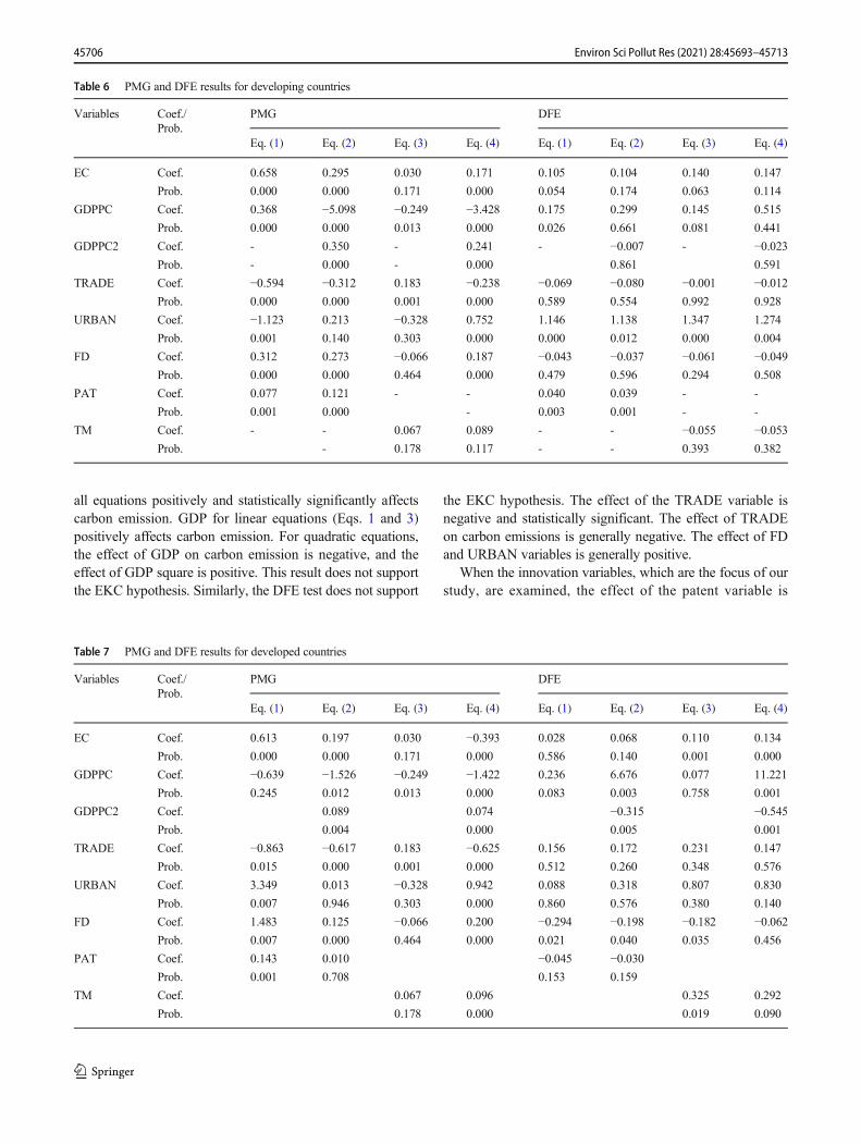
all equations positively and statistically significantly affectscarbon emission. GDP for linear equations (Eqs. 1 and 3)positively affects carbon emission. For quadratic equations,the effect of GDP on carbon emission is negative, and theeffect of GDP square is positive. This result does not supportthe EKC hypothesis. Similarly, the DFE test does not support

the EKC hypothesis. The effect of the TRADE variable isnegative and statistically significant. The effect of TRADEon carbon emissions is generally negative. The effect of FDand URBAN variables is generally positive.

When the innovation variables, which are the focus of ourstudy, are examined, the effect of the patent variable is

Table 7 PMG and DFE results for developed countries

Variables Coef./Prob.

PMG DFE

Eq. (1) Eq. (2) Eq. (3) Eq. (4) Eq. (1) Eq. (2) Eq. (3) Eq. (4)

EC Coef. 0.613 0.197 0.030 −0.393 0.028 0.068 0.110 0.134

Prob. 0.000 0.000 0.171 0.000 0.586 0.140 0.001 0.000

GDPPC Coef. −0.639 −1.526 −0.249 −1.422 0.236 6.676 0.077 11.221

Prob. 0.245 0.012 0.013 0.000 0.083 0.003 0.758 0.001

GDPPC2 Coef. 0.089 0.074 −0.315 −0.545Prob. 0.004 0.000 0.005 0.001

TRADE Coef. −0.863 −0.617 0.183 −0.625 0.156 0.172 0.231 0.147

Prob. 0.015 0.000 0.001 0.000 0.512 0.260 0.348 0.576

URBAN Coef. 3.349 0.013 −0.328 0.942 0.088 0.318 0.807 0.830

Prob. 0.007 0.946 0.303 0.000 0.860 0.576 0.380 0.140

FD Coef. 1.483 0.125 −0.066 0.200 −0.294 −0.198 −0.182 −0.062Prob. 0.007 0.000 0.464 0.000 0.021 0.040 0.035 0.456

PAT Coef. 0.143 0.010 −0.045 −0.030Prob. 0.001 0.708 0.153 0.159

TM Coef. 0.067 0.096 0.325 0.292

Prob. 0.178 0.000 0.019 0.090

Table 6 PMG and DFE results for developing countries

Variables Coef./Prob.

PMG DFE

Eq. (1) Eq. (2) Eq. (3) Eq. (4) Eq. (1) Eq. (2) Eq. (3) Eq. (4)

EC Coef. 0.658 0.295 0.030 0.171 0.105 0.104 0.140 0.147

Prob. 0.000 0.000 0.171 0.000 0.054 0.174 0.063 0.114

GDPPC Coef. 0.368 −5.098 −0.249 −3.428 0.175 0.299 0.145 0.515

Prob. 0.000 0.000 0.013 0.000 0.026 0.661 0.081 0.441

GDPPC2 Coef. - 0.350 - 0.241 - −0.007 - −0.023Prob. - 0.000 - 0.000 0.861 0.591

TRADE Coef. −0.594 −0.312 0.183 −0.238 −0.069 −0.080 −0.001 −0.012Prob. 0.000 0.000 0.001 0.000 0.589 0.554 0.992 0.928

URBAN Coef. −1.123 0.213 −0.328 0.752 1.146 1.138 1.347 1.274

Prob. 0.001 0.140 0.303 0.000 0.000 0.012 0.000 0.004

FD Coef. 0.312 0.273 −0.066 0.187 −0.043 −0.037 −0.061 −0.049Prob. 0.000 0.000 0.464 0.000 0.479 0.596 0.294 0.508

PAT Coef. 0.077 0.121 - - 0.040 0.039 - -

Prob. 0.001 0.000 - 0.003 0.001 - -

TM Coef. - - 0.067 0.089 - - −0.055 −0.053Prob. - 0.178 0.117 - - 0.393 0.382


positive for both PMG and DFE tests and statistically signif-icant at 1% level. On the other hand, the effect of the trade-mark variable is statistically insignificant. Table 7 showsPMG and DFE results for developed countries.

In Table 7, it is seen that energy consumption has a gener-ally positive effect on carbon emission for both PMG andDFE tests. The PMG test does not support the EKC hypothe-sis, on the other hand, the DFE model supports the EKChypothesis. TRADE generally reduces carbon emissions forthe PMGmodel. URBAN and FD have statistically significantand positive effects according to the PMG model results. Forthe DFE model, TRADE and URBAN do not have a statisti-cally significant effect. For the DFE model, FD reduces car-bon emissions.

When the innovation variables are examined, the effect ofthe patent variable is positive for the PMG test and statisticallysignificant at 1% level. It is statistically insignificant for theDFE test. On the other hand, the effect of the trademark var-iable is statistically significant and positive for both PMG andDFE tests.

Robustness

In this study, firstly, cross-sectional dependency is checkedfor unit root test, and PANIC method is used as the mostupdated and appropriate method. In this method, 3 differentstatistics are used for robustness check. Panel modifiedSargan–Bhargava test results are also presented for the auto-correlation problem, especially as an important deficiency ofPANIC test statistics.

On the other hand, the cross-sectional dependency and het-erogeneity of the estimated equations are investigated in orderto determine the appropriate method for investigating the co-integration relationship. According to the findings, Pedronimethodology, which presents both group and panel statistics,and Durbin–Hausman methodologies that consider cross-sectional dependency and heterogeneity are used. Both unit roottests and co-integration test results provide consistent results.

In order to obtain long-term coefficients, we prefer PMGand DFE tests, which are methods suitable for the estimationequations. Autocorrelation and heteroscedasticity can causeresults to be biased and inconsistent for these methodologies.We analyzed estimation equations for autocorrelation andheteroscedasticity problems, and test results can be seen inAppendix 2. Modified Bhargava et al. Durbin–Watson andBaltagi–Wu (LBI) tests are preferred for autocorrelation.According to Baltagi (2008) if the modified Bhargava et al.Durbin–Watson and Baltagi–Wu (LBI) tests statistics are lessthan 2, there is a serious autocorrelation problem. Accordingto the results in Appendix 2, it is seen that the test statistics areclose to or above 2. On the other side, according toheteroscedasticity test results, the basic hypothesis stated thatthe variance is equal between the units for all equations is

rejected, and it is decided that there is a heteroscedasticityproblem. For prediction equations to tackle the problem ofheteroscedasticity, we use the estimators developed byArellano (1987), Froot (1989), and Rogers (1993), which pro-vide robust parameter estimates.

PMG and DFE test results generally support each other. Onthe other hand, different test statistics are also available.Therefore, we use Hausman test to investigate which of thePMG or DFE estimators are more effective. In this way, theeffective estimator has been determined. Hausman test resultsare seen in Appendix 3. According to the test results, it isconcluded that the DFE estimators are effective.

As a result, evidence has been reached in our study that fordeveloping countries, Kuznets hypothesis is not valid, and fordeveloped countries, Kuznets hypothesis is valid. For devel-oping countries, if the increase in innovation level is caused bythe increase in patents, it has a negative effect on carbon emis-sions from transportation. Trademark increase does not have astatistically significant effect on carbon emissions. The testresults for developed countries indicated that the patent in-crease does not have a statistically significant effect on carbonemissions and the trademark increase have a positive effect onthe carbon emission.

Conclusion

In this study, the impact of innovation on carbon emissionsoriginating from the transportation sector is analyzed in theMediterranean countries. Considering the IMF (2019) report,Mediterranean countries are divided into two groups as devel-oped and developing countries: 8 developing countries whosedata can be accessed (Albania, Algeria, Bosnia andHerzegovina, Croatia, Egypt, Morocco, Tunisia, andTurkey) and 6 developed countries (Cyprus, France, Greece,Israel, Italy, and Spain). The analysis period has been deter-mined as 1997–2017 for developing countries and 2003–2017for developed countries, depending on the availability of data.

In our study, patent applications and trademark applica-tions, which are frequently used in the literature, were usedas innovation indicators. The estimation equations for eachinnovation indicator were created both linearly and quadraticlinearly to test the Kuznets hypothesis. Hence, 4 equationswere used in total. We concluded that while the Kuznets hy-pothesis is not valid for developing countries, it is valid fordeveloped countries. For developing countries, the increase inthe level of innovation has a positive impact on carbon emis-sions due to transport if the innovation results from the in-crease in patents. However, the trademark increase does nothave a statistically significant effect on carbon emissions. Theempirical results of the developed countries indicated that thepatent increase does not have a statistically significant effectand the trademark increase has a positive effect on carbon


emission. As the development level of the countries increases,the demand for personal vehicles also increases. In the devel-oped countries, the income per capita is high enough to haveown car. Therefore, as Erdoğan et al. (2020) pointed, althougha relative decrease in CO2 emissions from vehicles is observedthrough energy-saving innovation technologies and energyefficiency in the transportation sector, parallel to the increas-ing national income, having more personal vehicles, and driv-ing more bring more energy consumption in the developedMediterranean countries. Hence, to decrease the CO2 emis-sions in the Mediterranean countries, environment-friendlyinnovation technologies should be improved. However, par-allel to Rennings’ (2000) findings, it should be noted that thenew model of environment-friendly vehicles needs infrastruc-ture investments for adaptation and diffusion. Therefore, con-venient infrastructure investments should be initiated such ashaving widespread charging stations and technological im-provement to compete with their conventional counterparts.

Besides, conventional car owners should be encouraged toconsume less pollutive fuels, and the government should ini-tiate regulations and measures to control low-quality pollutingfuels. Furthermore, environment-friendly vehicles such aselectric vehicles should be widespread through tax incentivesand other supports.

In the future, the effects of innovation on CO2 emissions ona sectorial basis can be an important subject for researches.Not only the sectors that contribute to the global CO2 emis-sions but also less pollutive sectors can be included in thestudies. Besides, different sectors and different country groupscan be included in the forthcoming studies. It may be wise toapply more sophisticated econometric models in order toreach alternative results that have never been reached before.This may provide possibility to make comparisons and esti-mations of econometric models. The findings of the re-searches on a sectoral basis may also provide a positive con-tribution to policy makers.

Appendix 1

Table 8 PANIC unit root test

Tests Intercept Int&Trend Intercept Int&Trend

Stat. p-value

Stat. p-value

Stat. p-value

Stat. p-value

Developing countriesEC LNGDPPC

Pa −0.708 0.240 −1.730 0.042 1.880 0.970 0.551 0.709Pb −0.537 0.296 −1.340 0.090 2.555 0.995 0.630 0.736PMSB −0.589 0.278 −0.848 0.198 2.219 0.987 0.712 0.762

LNTM LNPATPa −4.437 0.000 −1.412 0.079 −1.061 0.144 −0.570 0.284Pb −2.165 0.015 −1.159 0.123 −0.846 0.199 −0.515 0.303PMSB −1.382 0.084 −0.775 0.219 −0.480 0.316 −0.352 0.363

LNTRADE LNTCO2Pa −3.520 0.000 −0.559 0.288 −1.869 0.031 1.047 0.852Pb −1.815 0.035 −0.508 0.306 −1.549 0.061 1.445 0.926PMSB −1.229 0.110 −0.383 0.351 −0.561 0.288 1.947 0.974

LNGDPPC2 LNURBANPa 1.966 0.975 0.220 0.587 −4.528 0.000 −0.989 0.161Pb 2.633 0.996 0.233 0.592 −2.338 0.010 −0.826 0.204PMSB 2.077 0.981 0.255 0.601 −1.052 0.146 −0.591 0.277

LNFDPa −3.556 0.000 −1.333 0.091Pb −1.661 0.048 −1.105 0.135PMSB −1.394 0.082 −0.763 0.223

Developed countriesEC GDPPC

Pa 0.617 0.731 −1.356 0.088 −1.052 0.146 −0.855 0.196Pb 20.497 1.000 −1.225 0.110 −64.530 0.000 −0.826 0.204PMSB 1.792 0.963 −0.544 0.293 −0.491 0.312 −0.239 0.406

TM PATPa 0.752 0.774 1.544 0.939 1.420 0.922 −1.706 0.044Pb 38.234 1.000 2.606 0.995 46.343 1.000 −1.540 0.062PMSB 6.885 1.000 4.823 1.000 1.155 0.876 −0.612 0.270


Appendix 2

Appendix 3

Table 8 (continued)

Tests Intercept Int&Trend Intercept Int&Trend

Stat. p-value

Stat. p-value

Stat. p-value

Stat. p-value

TRADE TCO2Pa −1.090 0.138 −1.126 0.130 −2.786 0.003 −0.481 0.315Pb −50.177 0.000 −1.065 0.143 −81.928 0.000 −0.485 0.314PMSB −0.069 0.473 −0.387 0.349 −0.871 0.192 0.004 0.502

GDPPC2 URBANPa 0.773 0.780 −0.080 0.468 −1.090 0.138 −1.443 0.075Pb 1.251 0.895 −0.087 0.465 −50.177 0.000 −1.275 0.101PMSB 2.099 0.982 0.510 0.695 −0.069 0.473 −0.613 0.270

FDPa 1.569 0.942 −1.468 0.071Pb 67.356 1.000 −1.341 0.090PMSB 0.853 0.803 −0.529 0.298

Table 9 Autocorrelation andheteroscedasticity test results Tests Eq. (1) Eq. (2) Eq. (3) Eq. (4)


Modified Bhargava et al. Durbin–Watson 1.682 1.705 1.696 1.675

Baltagi–Wu LBI 1.814 1.825 1.816 1.808

Chi2 227.2 200.4 212.3 265.7

Prob. 0.000 0.000 0.000 0.000

Developed countries

Modified Bhargava et al. Durbin–Watson 2.242 2.197 2.210 2.149

Baltagi–Wu LBI 2.294 2.267 2.267 2.238

Chi2 22.78 21.76 18.22 17.24

Prob. 0.000 0.001 0.005 0.008

Table 10 Hausman testresults Developing countries

Chi2 0.01 0.00 0.00 0.00

Prob. 1.00 1.00 1.00 1.00

Developed countries

Chi2 0.00 0.01 0.00 0.01

Prob. 1.00 1.00 1.00 1.00


Appendix 4

Table 11 The summary table for the literature review

Author(s) Period Country group Indicator(s) Method(s) Results

Innovation and CO2 emissionsJohnstone et al.

(2010)1978–2003 25 OECD countries R&D expenditures, electricity price,

growth of electricity consumption,EPO patent filings, environmentalpolicies

Panel data, negativebinomial fixed effectsmodels

Innovation increasesrenewable energyactivities

Fei et al. (2014) 1971–2010 Norway and NewZealand

Clean energy, economic growth, andCO2 emissions

Autoregressive distributedlag model, Grangercausality

Innovation reduces CO2

Irandoust (2016) 1975–2012 Nordic countries Technological innovation, renewableenergy growth, CO2 emissions

VAR model, Grangernon-causality

Innovation is Grangercause of renewableenergy

Zhang et al.(2017)

2000–2013 China Resource innovation, knowledgeinnovation, environmentalinnovation, and CO2 emissions

SGMM technique Innovation reduces CO2

Samargandi(2017)

1970–2014 Saudi Arabia Technological innovation, GDP, andCO2 emissions

ARDL Innovation reduces CO2

Mensah et al.(2018)

28 OECDcountries

1990–2014 GDP per capita, CO2 emissions,innovation

STIRPAT model Innovation reduces CO2

Kahouli (2018) 1990–2016 18 Mediterraneancountries

Electricity consumption, R&D stocks,CO2 emissions, and economicgrowth

Causality, SUR, 3SLS, andGMM techniques

Innovation is Grangercause of renewableenergy

Danish (2019) 1990–2016 59 Countries ICT, CO2 emissions Generalized least-squareapproach


Petrovic andLobanov(2020)

1981 and 2014 16 OECD countries R&D expenditures and CO2 emissions Nonparametric panel datatechnique,co-integration


Shahbaz et al.(2020)

1984–2018 China Technological innovations, carbonemissions

BARDL Innovation reduces CO2

Nguyen et al.(2020)

2000–2014 13 selected G-20 coun-tries

Energy price, foreign direct investment,trade openness, technology,innovation, and Co2

Full modified OLSapproach and quantilepanel regressions


Wen et al. (2020) 2000–2015 30 provinces of China Technological innovations, CO2 Moran’s I index and spatialeconometric models


Álvarez-Herránzaet al. (2017)

1990–2014 28 OECD countries Energy research development andgreenhouse gas emissions

ERD&D model Innovation does not reduceCO2

Amri et al. (2018) 1971–2014 Tunisia Technological innovation, trade,energy consumption, CO2

ARDL Innovation reduces CO2

Khattak et al.(2020)

1980–2016 BRICS countries Innovation, renewable energy, andGDP, CO2 emissions

Johansson Fisherco-integration

There is bidirectionalcausality betweeninnovation and CO2

Su and Moaniba(2017)

1976–2014 70 countries Patent count, carbon dioxide, otherGHG emissions, GDP andpopulation

Fixed effects binarylogistic regressions,ARDL

Reverse causality

Du et al. (2019b) 1996–2012 71 countries Technology innovations and CO2 Panel threshold model Innovation does not reduceCO2 in low regime andreduce in upper regime

Koçak andŞentürk Ulucak(2019)

2003–2015 OECD countries R&D expenditures and CO2 emissions STIRPAT model Innovation reduces CO2

Transportation and CO2 emissionsZhou et al. (2013) 2003–2009 China

30 regionsCO2 emissions and China’s transport

sectorDEA Transportation increases

CO2

Li et al. (2013) 1985–2007 China Vehicle fuel intensity, working vehiclestock, transport operator,industrialization level, economicgrowth, and CO2 emissions

Divisia index approach Transportation increasesCO2

Guo et al. (2014) 2005–2012 China Population, energy intensity, energystructure, and CO2 emission

Logarithmic mean Divisiaindex (LMDI) method

Transportation increasesCO2

Fan and Lei(2016)

1995–2012 Beijing, China Transportation intensity, energystructure, energy intensity, the

GFI model Transportation reducesCO2


Author contribution NDÇ: writing—original draft preparation and datacollection; AG: investigation, conceptualization, and methodology; SE:supervision; KA: investigation, writing—review and editing; DÇY: con-ceptualization, methodology, and formal analysis.

Data availability The data that support the findings of this study areavailable from the corresponding author upon reasonable request.

Declarations

Ethics approval and consent to participate Not applicable.

Consent for publication Not applicable.

Competing interests The authors declare no competing interests.

References

Álvarez-Herránza A, Balsalobreb D, Cantos JM, Shahbaz M (2017)Energy innovations-GHG emissions nexus: fresh empirical evi-dence from OECD countries. Energy Policy 101:90–100

Amri F, Bélaïd F, Roubaud R (2018) Does technological innovationimprove environmental sustainability in developing countries?Some evidence from Tunisia. The Journal of Energy andDevelopment, 44, No. 1/2 (Autumn 2018 and Spring 2019), 41–60

Arellano M (1987) Computing robust standart errors for within groupestimators. Oxf Bull Econ Stat 49(4):431–434

Bai J, Ng S (2004) A PANIC attack on unit roots and co-integration.Econometrica 74(4):1127–1177

Baltagi BH (2008) Econometric analysis of panel data, vol 4.Wiley, NewYork

Banister D (2005) Unsustainable transport, city transport in the new cen-tury. Routledge, Abingdon

Broughel J, Thierer A (2019) Technological innovation and economicgrowth: a brief report on the evidence. Mercatus Research,Mercatus Center at George Mason University, Arlington

Chang Y (2002) Nonlinear IV unit root tests in panels with cross-sectiondependency. J Econ 110:261–292

Chaudhry SM, Ahmed R, Shafiullah M, Huynh TLD (2020) The impactof carbon emissions on country risk: evidence from the G7 econo-mies. J Environ Manag 265:110533

Danish (2019) Effects of information and communication technology andreal income on CO2 emissions: the experience of countries alongBelt and Road. Telematics Inform 45:101300

Du H, Chen Z, Peng B, Southworth F, Ma S (2019a) What drives CO2

emissions from the transport sector? A linkage analysis. Energy 175:195–204

Du K, Li P, Yan Z (2019b) Do green technology innovations contributeto carbon dioxide emission reduction? Empirical evidence from pat-ent data. Technol Forecast Soc Chang 146:297–303

Erdoğan S, Gedikli A, Yılmaz AD, Haider A (2019a) Investigation ofenergy consumption–economic growth nexus: a note on MENAsample. Energy Rep 5:1281–1292

Erdoğan S, Yıldırım DÇ, Gedikli A (2019b) Investigation of causalityanalysis between economic growth and CO2 emissions: the case ofBRICS - T countries. Int J Energy Econ Policy 9(6):430–438

Erdoğan S, Yıldırım S, Yıldırım DÇ, Gedikli A (2020) The effects ofinnovation on sectoral carbon emissions: evidence from G20 coun-tries. J Environ Manag 267:110637

Fan F, Lei Y (2016) Decomposition analysis of energy-related carbonemissions from the transportation sector in Beijing. Transp ResPart D: Transp Environ 42:135–145

Fei Q, Rasiah R, Shen LJ (2014) The clean energy-growth nexus withCO2 emissions and technological innovation in Norway and NewZealand. Energy Environ 25(8):1323–1344

Froot KA (1989) Consistent covariance matrix estimation with cross-sectional dependence and heteroskedasticity in financial data. JFinanc Quant Anal 24(3):333–355

Georgatzi VV, Stamboulis Y, Vetsikas A (2020) Examining thedeterminants of CO2 emissions caused by the transport sec-tor: empirical evidence from 12 European countries. EconAnal Policy 65:11–20

Goulias D (2007) Development of high performance and innovative in-frastructure materials. In: Goulias KG (ed) Transport Science andTechnology. Elsevier, Oxford, pp 55–67

Table 11 (continued)

Author(s) Period Country group Indicator(s) Method(s) Results

output value of per unit trafficturnover, population, economicgrowth, and CO2

Wang and He(2017)

2007 to 2012 China CO2 marginal mitigation costs, CO2

emissions efficiency, economicefficiency, and productivity

Data envelopment analysisapproach

CO2 emissions efficiencyand marginal mitigationcost of CO2 emissionsare negativelycorrelated

Zhu and Du(2019)

1990–2016 Australia, Canada,China, India,Russia, and the USA

Economic output, population, CO2 LMDI decompositionmethod


Du et al. (2019a) 2002 to 2012 China Transportation sector and the Chineseeconomy

Hypothetical extractionmethod (HEM)

Road subsector increasedCO2while rail subsectormitigation in CO2

Khan et al. (2020) 1991–2017 Pakistan Construction, manufacturing,transportation, agriculture andservices sectors, CO2

Quantile regressionmethod


Georgatzi et al.(2020)

1994–2014 12 European countries CO2 emissions and transport sectorinvestments

Granger causality Transportation does nothave an effect on CO2


Greening LA, Greene DL, Difiglio C (2000) Energy efficiency andconsumption-the rebound effect—a survey. Energy Policy 28:389–401

Guo B, Geng Y, Franke B, Hao H, Liu Y, Chiu A (2014) UncoveringChina’s transport CO2 emission patterns at the regional level.Energy Policy 74:134–146

Herring H, Roy R (2007) Technological innovation, energy efficient de-sign and the rebound effect. Technovation 27(4):194–203

IEA (2009a) Transport, energy, and CO2, moving towards sustainability.France

IEA (2009b) Transport, Energy and CO2. Report, October 2009IEA (2019a) CO2 emissions from fuel combustion by sector 2017.

https://www.iea.org/data-and-statistics/charts/transport-sector-co2-emissions-by-mode-in-the-sustainable-development-scenario-2000-2030. Accessed 10 Jan 2021

IEA (2019b) Transport sector CO2 emissions by mode in the sustainabledevelopment scenario, 2000-2030, 22 November 2019. https://www.iea.org/data-and-statistics/charts/transport-sector-co2-emissions-by-mode-in-the-sustainable-development-scenario-2000-2030. Accessed 10 Jan 2021

IEA (2020a) Transport-improving the sustainability of passenger andfreight transport. https://www.iea.org/topics/transport. Accessed 10Jan 2021

IEA (2020b) Global energy review 2020. April 2020. https://www.iea.org/reports/global-energy-review-2020/global-energy-and-co2-emissions-in-2020. Accessed 10 Jan 2021

IMF (2019) World economic outlook, October 2019: Global manufactur-ing downturn, rising trade barriers. International Monetary Fund.Research Dept., Washington DC:USA

Irandoust M (2016) The renewable energy-growth nexus with carbonemissions and technological innovation: evidence from the Nordiccountries. Ecol Indic 69:118–125

Jiang Y, Zhou Z, Liu C (2018) The impact of public transportation oncarbon emissions: a panel quantile analysis based on Chinese pro-vincial data. Environ Sci Pollut Res 26:4000–4012

Jin L, Duan K, Tang X (2018) What is the relationship between techno-logical innovation and energy consumption? Empirical analysisbased on provincial panel data from China. Sustainability 10(145):1–13

Johnstone N, Haščič I, Popp D (2010) Renewable energy policies andtechnological innovation: evidence based on patent counts. EnvironResour Econ 45:133–155

Kahouli B (2018) The causality link between energy electricity consump-tion, CO2 emissions, R&D stocks and economic growth inMediterranean countries (MCs). Energy 145:388–399

Khan AN, En X, Raza MY, Khan NA, Ali A (2020) Sectorial study oftechnological progress and CO2 emission: insights from a develop-ing economy. Technol Forecast Soc Chang 151:119862

Khattak SI, Ahmad M, Khan Z, Khan A (2020) Exploring the impact ofinnovation, renewable energy consumption, and income on CO2emissions: new evidence from the BRICS economies. Environ SciPollut Res 27(12):13866–13881

Koçak E, Şentürk Ulucak Z (2019) The effect of energy R&D expendi-tures on CO2 emission reduction: estimation of the STIRPATmodelfor OECD countries. Environ Sci Pollut Res 26:14328–14338

Le Quéré C, Jackson RB, Jones MW, Smith AJP, Abernethy S, AndrewRM et al (2020) Temporary reduction in daily global CO2 emissionsduring the COVID-19 forced confinement. Nat Clim Chang 10:647–653

Lemoine D (2019) General equilibrium rebound from energy efficiencyinnovation. NBER Working Paper, No. 25172, September 2019

Li H, LuY, Zhang J,Wang T (2013) Trends in road freight transportationcarbon dioxide emissions and policies in China. Energy Policy 57:99–106

Maradana RP, Pradhan RP, Dash S, Gaurav K, Jayakumar M, ChatterjeeD (2017) Does innovation promote economic growth? Evidencefrom European countries. J Innov Entrep 6(1):1–23

Mensah CN, Long X, Boamah KB, Bediako IA, Dauda L, Salman M(2018) The effect of innovation on CO2 emissions of OECD coun-tries from 1990 to 2014. Environ Sci Pollut Res 25:29678–29698

Moon R, Perron B (2004) Testing for a unit root in panels with dynamicfactors. J Econ 122:81–126

Muntean M, Guizzardi D, Schaaf E, Crippa M, Solazzo E, Olivier JGJ,Vignati E (2018) Fossil CO2 emissions of all world countries - 2018Report. EUR 29433 EN, Publications Office of the European Union,Luxembourg

Nasir MA, Huynh TLD, Tram HTX (2019) Role of financial develop-ment, economic growth & foreign direct investment in driving cli-mate change: a case of emerging ASEAN. J Environ Manag 242:131–141

Newey WK, West KD (1994) Automatic lag selection in covariancematrix estimation. Rev Econ Stud 61(4):631–653. https://doi.org/10.2307/2297912

Nguyen TT, Pham TAT, Tram HTX (2020) Role of information andcommunication technologies and innovation in driving carbon emis-sions and economic growth in selected G-20 countries. J EnvironManag 261:110162

O’Connell PGJ (1998) The overvaluation of purchasing power parity. JInt Econ 44(1):1–19

Pece AM, Simona OEO, Salisteanu F (2015) Innovation and economicgrowth: an empirical analysis for CEE countries. Procedia EconFinance 26:461–467

Pedroni P (2004) Panel cointegration: asymtotic and finite sample prop-erties of pooled time series tests with an application to the PPPhypothesis. Econometric Theory 20:597–625

PesaranMH (2004) General diagnostic tests for cross-section dependencein panels. Cambridge Working Papers in Economics, 435

Pesaran MH (2007) A simple unit root test in the presence of cross-section dependence. J Appl Econ 22:265–312

Pesaran MH, Yamagata T (2008) Testing slope homogeneity in largepanels. J Econ 142(1):50–93

Pesaran MH, Shin Y, Smith RP (1999) Pooled mean group estimation ofdynamic heterogeneous panels. J Am Stat Assoc 94(446):621–634

Pesaran MH, Smith R (1995) Estimating long-run relationships fromdynamic heterogeneous panels. J Econ 68:79–113

Petrovic P, Lobanov MM (2020) The impact of R&D expenditures onCO2 emissions: evidence from sixteen OECD countries. J CleanProd 248:119187

Pham NM, Huynh TLD, Nasir MA (2020) Environmental consequencesof population, affluence and technological progress for Europeancountries: a Malthusian view. J Environ Manag 260:110143

Rennings K (2000) Redefining innovation-eco-innovation research andthe contribution from ecological economics. Ecol Econ 32:319–332

Ritchie H. Roser M (2020) Emissions by sectors. Our World in Data.https://ourworldindata.org/emissions-by-sector#annual-greenhouse-gas-emissions-by-sector. Accessed 10 Jan 2021

Roger EM (1983) Diffusion of innovation, 3rd edn. The Free Press, NewYork

RogersWH (1993) Regression standard errors in clustered samples. StataTech Bull 13:19–23

Rosenberg N (2004) Innovation and economic growth. OECD. https://www.oecd.org/cfe/tourism/34267902.pdf. Accessed 10 Jan 2021

Rowland, F. S.; Bruce, J. P; Graedel, T. E.; Reck, R. A.; Sperling, D.; andWaltn, C. M. (1998). Atmospheric change and the North Americantransportation sector: summary of a trilateral workshop. IncidentalReport No. IR98-1, The Royal Society of Canada, 1–24

Samargandi N (2017) Sector value addition, technology and CO2 emis-sions in Saudi Arabia. Renew Sust Energ Rev 78:868–877

Schumpeter JA (2000) Entrepreneurship as innovation. The University ofIllinois at Urbana-Champaign’s Academy for Entrepreneurial


https://www.iea.org/data-and-statistics/charts/transport-sector-co2-emissions-by-mode-in-the-sustainable-development-scenario-2000-2030







https://www.iea.org/topics/transport

https://www.iea.org/reports/global-energy-review-2020/global-energy-and-co2-emissions-in-2020



https://doi.org/10.2307/2297912

https://doi.org/10.2307/2297912

https://ourworldindata.org/emissions-by-sector#annual-greenhouse-gas-emissions-by-sector

https://ourworldindata.org/emissions-by-sector#annual-greenhouse-gas-emissions-by-sector

https://www.oecd.org/cfe/tourism/34267902.pdf

https://www.oecd.org/cfe/tourism/34267902.pdf

Leadership Historical Research Reference in Entrepreneurship,Available at SSRN: https://ssrn.com/abstract=1512266. Accessed10 Jan 2021

ShahbazM, Raghutla C, SongM, Zameer H, Jiao Z (2020) Public-privatepartnership investment in energy as new determinant of CO2 emis-sions: the role of technological innovations in China. Energy Econ86:104664

SuH-N,Moaniba IM (2017) Does innovation respond to climate change?Empirical evidence from patents and greenhouse gas emissions.Technol Forecast Soc Chang 122:49–62

Swamy PAVB (1970) Efficient inference in a random coefficient regres-sion model. Econometrica 38:311–323

Teter J, Tattini J, Petropoulos A (2020) Tracking transport 2020- moreefforts needed. Tracking Report, IEA, May 2020. https://www.iea.org/reports/tracking-transport-2020#. Accessed 10 Jan 2021

The United States Environmental Protection Agency (EPA) (2019)Source of greenhouse emissions, transportation sector emissions.https://www.epa.gov/ghgemissions/sources-greenhouse-gas-emissions#carbon-dioxide. Accessed 10 Jan 2021

Ulku H (2004) R&D, Innovation, and economic growth: an empiricalanalysis. IMF Working Paper, WP/04/185, September 2004

UNCED (1992) Sustainabel development goals platform, Agenda 21.https://sustainabledevelopment.un.org/outcomedocuments/agenda21. Accessed 10 Jan 2021

Wang Z, HeW (2017) CO2 emissions efficiency and marginal abatementcosts of the regional transportation sectors in China. Transp Res PartD: Transp Environ 50:83–97

WenQ, ChenY, Hong J, ChenY,Ni D, Shen Q (2020) Spillover effect oftechnological innovation on CO2 emissions in China’s constructionindustry. Build Environ 171:106653

Westerlund J (2008) Panel co-integration tests of the Fisher effect. J ApplEcon 23(2):193–223

Yıldırım S, Gedikli A, Erdoğan S, Yıldırım DÇ (2020) Natural resourcesrents-financial development nexus: evidence from sixteen develop-ing countries. Res Policy 68:101705

Zhang Y-J, Peng Y-L, Ma C-Q, Shen B (2017) Can environmental inno-vation facilitate carbon emissions reduction? Evidence from China.Energy Policy 100:18–28

Zhou G, ChungW, Zhang X (2013) A study of carbon dioxide emissionsperformance of China’s transport sector. Energy 50:302–314

Zhu C, DuW (2019) A research on driving factors of carbon emissions ofroad transportation industry in six Asia-Pacific countries based onthe LMDI decomposition method. Energies 12(4152):1–19

Publisher’s note Springer Nature remains neutral with regard to jurisdic-tional claims in published maps and institutional affiliations.


https://ssrn.com/abstract=1512266

https://www.iea.org/reports/tracking-transport-2020

https://www.iea.org/reports/tracking-transport-2020

https://www.epa.gov/ghgemissions/sources-greenhouse-gas-emissions#carbon-dioxide

https://www.epa.gov/ghgemissions/sources-greenhouse-gas-emissions#carbon-dioxide

https://doi.org/10.2307/2297912

https://doi.org/10.2307/2297912

Documents

A comparative analysis of the relationship between