Embed Size (px)
Citation preview
A fourier pseudospectral method forsome computational aeroacoustics
problems
Xun Huang and Xin Zhangdagger
Aeronautics and Astronautics School of Engineering Sciences
University of Southampton Southampton SO17 1BJ UK
ABSTRACTA Fourier pseudospectral time-domain method is applied to wave propagation problems pertinentto computational aeroacoustics The original algorithm of the Fourier pseudospectral time-domain method works for periodical problems without the interaction with physical boundariesIn this paper we develop a slip wall boundary condition combined with buffer zone technique tosolve some non-periodical problems For a linear sound propagation problem whose governingequations could be transferred to ordinary differential equations in pseudospectral space a newalgorithm only requiring time stepping is developed and tested For other wave propagationproblems the original algorithm has to be employed and the developed slip wall boundarycondition still works The accuracy of the presented numerical algorithm is validated bybenchmark problems and the efficiency is assessed by comparing with high-order finitedifference methods It is indicated that the Fourier pseudospectral time-domain method timestepping method slip wall and absorbing boundary conditions combine together to form a fully-fledged computational algorithm
1 INTRODUCTIONPseudospectral time-domain methods were developed to achieve spectral level accuracyin numerical solutions of the partial differential equations So far a number of attemptswere made to apply numerical algorithms based on the pseudospectral time-domainmethods to simulate various wave phenomena such as electromagnetic seismic andacoustic waves [1 2 3 4] with various degrees of success It is accepted thatpseudospectral time-domain methods have high spatial resolution that meets therequirements of numerical simulation of aeroacoustic phenomena In this work weapply a class of pseudospectral time-domain method based on the Fouriertransformation to sound propagation problems commonly encountered in aeroacoustics
aeroacoustics volume 5 middot number 3 middot 2006 ndash pages 279 ndash 294 279
Graduate Student Aeronautics and Astronautics Email xungersotonacukdagger Professor Aeronautics and Astronautics Email xzhangsotonacuk
JA-53_04_Xun Huang 16806 231 pm Page 279
The basic idea of pseudospectral time-domain method is to represent the spatialderivatives in the spectral domain by a set of basis functions There are two categoriesof orthogonal functions which are commonly used as the basis functions One is theFourier series that can be used in periodical problems [1] The other and morecommonly used function is the Chebyshev polynomials The advantage of theChebyshev pseudospectral time-domain method lies in its ability to deal with non-periodic problems on non-uniform and multi-domain computational grids [5 6] at thecost of computational efficiency On the other hand the Fourier pseudospectral time-domain method is simple to implement and has comparatively low computing cost Itdoes though have certain restrictions eg solutions should satisfy Lipschitz conditionthe method has to work on a uniform grid and is only applicable to periodical problemsThe current work addresses some of these issuesrestrictions in the development ofnumerical algorithms based on the Fourier pseudospectral time-domain method underthe context of computational aeroacoustics
In the implementation of a Fourier pseudospectral time-domain method discreteFourier transforms are applied to get a spectral pair of the original variables The spatialderivatives of the original variables can be approximated through multiplications of thespatial sampling frequency and spectral pair of the variables In the case of a one-dimensional problem the spectral pair of the original variable y(x t) is Y
ndash(kx t) and thespectral pair of its derivative party(xt)partx is jkx Y
ndash(kx t) where kx is the wavenumberrather than the meaning of sampling frequency in the temporal sequence According to the Nyquist criteria only 2 points-per-wavelength are required to obtain exactresults [7] This compares with other high-order finite difference methods such ascompact schemes where typically 8 or more points-per-wavelength are required to meetthe dispersion requirement
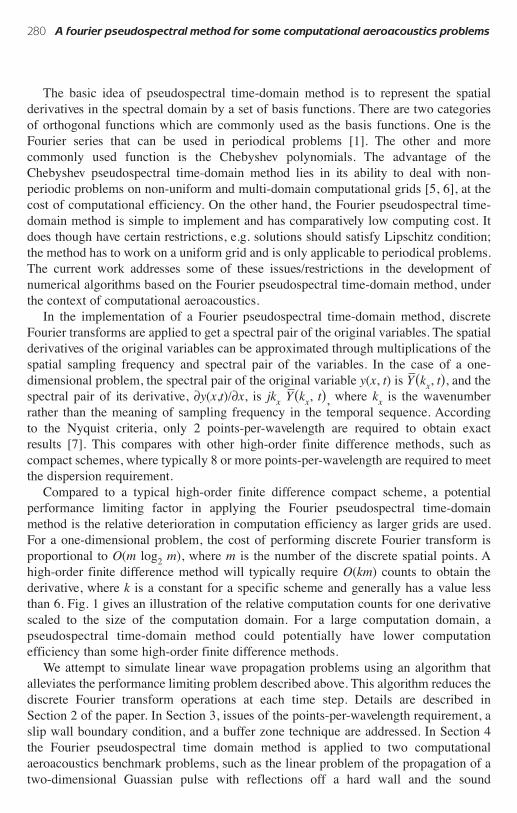
Compared to a typical high-order finite difference compact scheme a potentialperformance limiting factor in applying the Fourier pseudospectral time-domainmethod is the relative deterioration in computation efficiency as larger grids are usedFor a one-dimensional problem the cost of performing discrete Fourier transform isproportional to O(m log2 m) where m is the number of the discrete spatial points Ahigh-order finite difference method will typically require O(km) counts to obtain thederivative where k is a constant for a specific scheme and generally has a value lessthan 6 Fig 1 gives an illustration of the relative computation counts for one derivativescaled to the size of the computation domain For a large computation domain apseudospectral time-domain method could potentially have lower computationefficiency than some high-order finite difference methods
We attempt to simulate linear wave propagation problems using an algorithm thatalleviates the performance limiting problem described above This algorithm reduces thediscrete Fourier transform operations at each time step Details are described in Section 2 of the paper In Section 3 issues of the points-per-wavelength requirement aslip wall boundary condition and a buffer zone technique are addressed In Section 4the Fourier pseudospectral time domain method is applied to two computationalaeroacoustics benchmark problems such as the linear problem of the propagation of atwo-dimensional Guassian pulse with reflections off a hard wall and the sound
280 A fourier pseudospectral method for some computational aeroacoustics problems
JA-53_04_Xun Huang 16806 231 pm Page 280
propagation of an open rotor [8 9] A summary of the present work is provided inSection 5
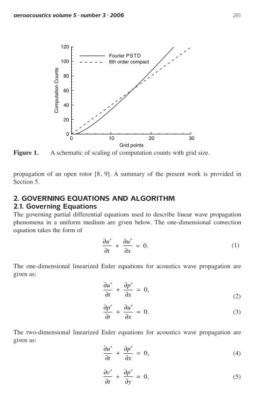
2 GOVERNING EQUATIONS AND ALGORITHM21 Governing EquationsThe governing partial differential equations used to describe linear wave propagationphenomena in a uniform medium are given below The one-dimensional convectionequation takes the form of
(1)
The one-dimensional linearized Euler equations for acoustics wave propagation aregiven as
(2)
(3)
The two-dimensional linearized Euler equations for acoustics wave propagation aregiven as
(4)
(5)part primepart
+part primepart
=v
t
p
y0
part primepart
+part primepart
=u
t
p
x0
part primepart
+part primepart
=p
t
u
x0
part primepart
+part primepart
=u
t
p
x0
part primepart
+part primepart
=u
t
u
x0
aeroacoustics volume 5 middot number 3 middot 2006 281
Fourier PSTD6th order compact100
80
60
40
20
10 20
Com
puta
tion
Cou
nts
120
00 30
Grid points
Figure 1 A schematic of scaling of computation counts with grid size
JA-53_04_Xun Huang 16806 231 pm Page 281
(6)
In the above equations t is the time x and y are the Cartesian coordinates uprime and vprime arevelocity perturbations and pprime is the pressure perturbation For the rest of the paper theprime sign will be dropped for convenience The fluid is modelled as a perfect gas andall variables are nondimensionalised using a reference length L a reference soundspeed a and a reference density ρ
22 An Algorithm in the Pseudospectral DomainWith the assumption that the spatial domain is periodical the one-dimensionalconvection equation Eq (1) can be transformed to
(7)
where Undash(kx t) is the pseudospectral pair for u(xt) and kx is the wavenumber in the x
direction For this problem an efficient algorithm can be employed to integrate Eq (7)directly to the new time step t + k∆t as an ordinary differential equation to yield Undash(kx t + k∆t) by using a suitable time-stepping scheme eg a low-dissipation
and low-dispersion Runge-Kutta scheme [10] Temporal solution is obtained byapplying an inverse Fourier transform to U
ndash(kx t + k∆t) producing an updated solutionu(xt + k∆t)
Following the same approach the one-dimensional linear wave equations aretransformed by the Fourier pseudospectral time-domain method to
(8)
(9)
where Pndash(kx t) and U
ndash(kx t) are the pseudospectral pair for the pressure perturbationp(xt) and velocity perturbation u(xt) respectively
The transformed two-dimensional linear wave equations are as follows
(10)
(11)dV k k t
dtjk P k k t
x y
y x y
( )+ ( ) = 0
dU k k t
dtjk P k k t
x y
x x y
( )+ ( ) = 0
dP k t
dtjk U k tx
x x
( )+ ( ) = 0
dU k t
dtjk P k tx
x x
( )+ ( ) = 0
dU k t
dtjk U k tx
x x
( )+ ( ) = 0
part primepart
+part primepart
+part primepart
=p
t
u
x
v
y0
282 A fourier pseudospectral method for some computational aeroacoustics problems
JA-53_04_Xun Huang 16806 231 pm Page 282
(12)
In Eqs (10 ndash 12) and are the two-dimensionalFourier transforms of the velocity perturbations u(xyt) and v(xyt) and pressureperturbation p(xyt) respectively Eqs (8ndash12) could be stepped in the spectral domaindirectly as well The above procedure can be applied to linear wave propagationequations with an underline mean flow to obtain and solve the transformed ordinarydifferential equations in pseudospectral domain
23 Performance AnalysisThe original algorithms of Fourier pseudospectral time domain method [6 7] has thefollowing form
(13)
where DFT and IDFT denote forward and inverse discrete Fourier transforms Otherthan the algorithm presented in section 22 this procedure is much more general Butthe forward and inverse discrete Fourier transforms will have to be used at each timestep to obtain the spatial derivatives
As mentioned in section 22 some computational aeroacoustics applications couldbe solved as ordinary differential equations in the forms of Eqs (7ndash12) For this typeof problems the approach adopted in this work is to apply discrete Fourier transformonly at the start of the computation The computation cost for the spatial derivatives ateach time step is removed within this procedure
In the case of a one-dimensional computational domain of m grid points the fastFourier transform algorithm requires operations in the order of O(m log2 (m)) a typicallow-dissipation and low-dispersion Runge-Kutta scheme requires operations in theorder of O(4m) and a typical prefactored compact schemersquos computational complexityis in the order of O(6m) [11] Consequently it can be estimated that for each time stepthe cost of a high-order finite difference method is in the order of O(10m) and theFourier pseudospectral time domain method of the original algorithm (Eq (13)) needscomputation counts in the order of O(m log2 m + 4m) By comparison the newcomputation procedure only requires operations in the order of O(4m) In fact it wasacknowledged that for some applications the early algorithm for the Fourierpseudospectral time domain method had a comparable computing speed to an efficientfinite difference scheme [12] even if a coarser grid was employed
3 ISSUES AND SOLUTIONSThere are several issues in applying Fourier pseudospectral time domain method tocomputational aeroacoustics problems such as resolution requirement and boundary
du
dtIDFT jk DFT f xi
x i i+ ( ( ( ))) 0=
P k k tx y ( )U k k t V k k tx y x y ( ) ( )
dP k k t
dtjk U k k t jk V k k t
x y
x x y y x y
( )+ ( ) + ( ) = 0
aeroacoustics volume 5 middot number 3 middot 2006 283
JA-53_04_Xun Huang 16806 231 pm Page 283
conditions These are discussed in this section The discussions apply to both algorithmsof the pseudospectral time domain method
31 Points-per-wavelength RequirementFor the Fourier pseudospectral time domain method a grid resolution of 2 points-per-wavelength is enough Results in Fig 2 presented demonstrate this point In thisexercise the one-dimensional advection equation (Eq (1)) with initial condition
of is solved Two resolutions are employed points-per-wavelength of 4 and 2 The computed results compare well with the analytical solutions
32 Hard-wall Boundary ConditionThe Fourier pseudospectral time domain method can be used to solve computationalaeroacoustics problems effectively with high spatial resolution The same property canbe found in Schultenrsquos characteristic method [13] However the characteristic methodcould not solve problems with the presence of solid bodies and simulate the resultedsound reflection
Based on the idea of generalized function [14] we now supply a hard-wall conditionfor the Fourier pseudospectral method For simplicity the one-dimensional wavepropagation Eqs (2ndash3) are used in the derivation We assume a stationary hard-wallcondition on the left boundary of the computation domain at x = 0 The hard-wallcondition suggests zero normal velocity at the wall To ensure a correct velocity field thefollowing condition needs to be enforced
(14)uu u
( )( ) ( )
00 0
20=
+ + minus=
u einit
x= minus minus 0 54 2 50 2
log( )( )
284 A fourier pseudospectral method for some computational aeroacoustics problems
(a) (b)
06
06
07
04
03
02
89 90x x
91
01
0
ndash01
Analytical solutionFourier PSTD Fourier PSTD
u
06
06
07
04
03
02
89 90 91
01
0
ndash01
Analytical solution
u
88 9288 92
Figure 2 One-dimensional Gaussian pulse propagation with low points-per-wavelength (a) PPW = 4 ∆t ∆x = 01 steps = 200 (b) PPW = 2 ∆t ∆x = 02 steps = 100
JA-53_04_Xun Huang 16806 231 pm Page 284
Eq (3) can be re-casted using the idea of generalized derivative for functions withdiscontinuities [14] to
(15)
Eq (15) can be transferred by a discrete Fourier transform to
(16)
where u(0+ t) is approximated by u(0t) which is obtained from an inverse discreteFourier transform operating on in each step
An example of the application with hard-wall condition is shown in Fig 3 where aone-dimensional wave is reflected from a hard wall at the left boundary The initial
condition is a Gaussian pulse defined by Eqs (8)and (16) are used to obtain the solutions Comparison is made with a fourth-orderdispersion-relation-preserving (DRP) scheme [15] In the most part two results agreewell but a rewrap wave appears when the Fourier pseudospectral time domain methodis used It is generated by the periodical boundary condition and can be absorbed by thetechnique described in the next section
33 Absorbing Condition for Rewrap WavesThe original Fourier pseudospectral time domain method works for problems withperiodical boundaries When the periodical assumption is not satisfied wave rewrapphenomenon will appear and contaminate the solutions in the computation domain Inthis work an explicit form of buffer zone techniques [16] is applied to absorb thereflected waves The buffer zone technique works in the spatial domain and
p e uinit
x
init= =minus = 0 5 02 20 92
log( )( )
U k tx ( )
part ( )part
+ ( ) ++
=P k t
tjk U k t
u t
xx
x x
( )
2 00
∆
partpart
+part
part+ + minus minus[ ] =
p x t
t
u x t
xu t u t x
( ) ( )( ) ( ) ( ) 0 0 0δ
aeroacoustics volume 5 middot number 3 middot 2006 285
(a) (b)
05
04
03
02
01
0
500
p
x100 150 200
ndash01
05
04
03
02
01
0
500
p
x100 150 200
ndash01
PSTDDRP
PSTDDRP
Figure 3 One-dimensional Gaussian pulse reflected by a left hard-wall withoutbuffer zone (a) Steps = 10 (b) Steps = 150
JA-53_04_Xun Huang 16806 231 pm Page 285
consequently the new algorithm for the Fourier pseudospectral time domain methodrequires more operation counts The exact number depends on the width of the bufferzone there is therefore a trade-off between memory and speed
In the implementation the solution vector is explicitly damped after every severaltime step by
(17)
where is the solution vector computed after regular time steps and F0 isthe target solution The damping coefficient σ varies according to the function
(18)
where L is the width of the buffer zone x is the distance from the inner boundary of thebuffer zone and σmax and β are set to 10 and 30 respectively In this work the targetsolution F0 is set to 0
4 APPLICATIONS TO BENCHMARK PROBLEMSThe aforementioned method is applied to two benchmark test cases Results anddiscussions are given here In the first case a two-dimensional Gaussian pulsepropagation problem with hard-wall and absorbing boundaries was computedemploying temporal integration directly on pseudospectral space In the second case thealgorithm in the form of Eq (13) was used to solve for an open rotor problem withnonlinear terms
41 Wave Propagation and ReflectionThis case is the first problem of category 4 that is defined at first computationalaeroacoustics workshop [8] The initial condition is a Gaussian acoustic pulse given by
(19)
uinit = 0 (20)
vinit = 0 (21)
Eqs (10ndash12) are used to solve the problem ∆t ∆x is set to 05 Results are presentedin Fig 4 The hard-wall boundary condition on the bottom boundary appears to havereproduced the reflected waves off the bottom wall In this exercise the length of thebuffer zone is set to 10 grid points In the current computation the buffer zone is notupdated at each time step Instead the solutions inside the buffer zone are updated atregular step intervals eg once every 2 or 4 steps to save computing time furthermoreThe algorithm employed for this exercise can be found in the appendix
p einit
x y= minus + + log( ) ( )
2 0 6 0 0062 2
σ σβ
( ) maxxx L
L= minus
minus1
F( )x t t+ ∆
F F F F( ) ( ) ( ) ( )x t t x t t x t t x+ = + minus + minus ∆ ∆ ∆σ 0
286 A fourier pseudospectral method for some computational aeroacoustics problems
JA-53_04_Xun Huang 16806 231 pm Page 286
The pressure distribution along the x = 0 axis is given in Fig 5 and compared withthe prediction given by a prefactored compact scheme [11] The computing time t andL2 error against to an analytical solution of linearized Euler equations [15] are listed inTable 1 where the spatial resolution is low from around 3 points-per-wavelength to 12points-per-wavelength
aeroacoustics volume 5 middot number 3 middot 2006 287
06
04
02
0
ndash02
ndash04
ndash06
ndash06 ndash04 ndash02 0 02 04 06 08
032
026
020
014
008
002
ndash004
ndash010
06
04
02
0
ndash02
ndash04
ndash06
ndash06 ndash04 ndash02 0 02 04 06 08
P
032
026
020
014
008
002
ndash004
ndash010
P
06
04
02
0
ndash02
ndash04
ndash06
ndash08 ndash06 ndash04 ndash02 0 02 04 06 08 1
032
026
020
014
008
002
ndash004
ndash010
06
04
02
0
ndash02
ndash04
ndash06
ndash06 ndash04 ndash02 0 02 04 06 08
P
032
026
020
014
008
002
ndash004
ndash010
P
x
08
Buffer zone Buffer zone
Buf
fer
zone
Buf
fer
zone
Buffer zone
Buffer zone
ndash08
y
08
ndash08
y
ndash08 1
x
ndash08 1x
08
ndash08y
ndash08 1x
08
ndash08
y
(a) (b)
(c) (d)
Figure 4 The propagation of a two-dimensional Gaussian pulse (a) t = 025without buffer zone (b) t = 04 without buffer zone (c) t = 025 bufferzone (d) t = 04 buffer zone
Table 1 Computing time t and L2 error of the first benchmark problem
Schemes 16 timestimes 16 64 timestimes 64
Compact t = 155s Err = 00425 t = 91s Err = 00013Pseudospectral (no buffer zone) t = 044s Err = 00938 t = 26s Err = 00825Pseudospectral (buffer zone) t = 048s Err = 00275 t = 28s Err = 00075
JA-53_04_Xun Huang 16806 231 pm Page 287
It has been discovered that with Fourier pseudospectral time domain method if abuffer zone is not applied wave rewraping will contaminate the solutions However ifthe rewrap wave is not considered in computing L2 errors over two grids they are00107 and 000083 correspondingly indicating the pseudospectral method is actuallymore exact than the compact scheme Fig 4(cndashd) and Fig 5(b) illustrate that a bufferzone keeps removing the rewrap wave The agreement is generally good as wellHowever the buffer zone affects the spectra of the solution near the hard wall as itabsorbs the rewrap wave It has been found that this difference will remain stable as thesolution develops L2 error results in Table 1 also indicate that the buffer zone doesaffect the accuracy of the Fourier pseudospectral method But for the majority of thedomain there are no significant differences in the solutions (see Fig 5(b)) Fig 6 alsopresents a comparison between the Fourier pseudospectral time domain method and theprefactored compact scheme after 110 time iterations
In terms of computation efficiency the Fourier pseudospectral method with orwithout a buffer zone represents a saving of up to 200 compared with the prefactoredcompact scheme
42 Open RotorThe second test case is that of the open rotor noise defined in category 2 benchmarkproblem at third computational aeroacoustics workshop [9] It has nonlinear sourceterms and could not be described in pseudospectral domain accordingly The simplifiedalgorithm using a temporal stepping directly on Eqs (7ndash12) is not applicable hereConsequently the original algorithm in the form of Eq (13) is used to show theeffectiveness of the Fourier pseudospectral method for general problems
The governing equations in cylindrical coordinates and the definitions of the problemare as follows
288 A fourier pseudospectral method for some computational aeroacoustics problems
(a) (b)
Compact Scheme02
0
0 02 04 06
01
ndash01
ndash02ndash04
Fourier PSTD
08ndash06y
03
ndash02
p
Compact Scheme02
0
0 02
01
ndash01
ndash02ndash04ndash06
Fourier PSTD
04ndash08y
03
ndash02
pFigure 5 A comparison of two-dimensional Gaussian pulse propagation predicted
by the Fourier pseudospectral method and a prefactored compact schemePressures along the x = 0 axis (a) t = 04 without buffer zone (b) t = 04buffer zone
JA-53_04_Xun Huang 16806 231 pm Page 288
(22)
(23)
(24)
(25)
where x is the axial coordinate r the radial coordinate and Φ the azimuthal angle uvware the velocity perturbations in the xrΦ directions respectively and p is the pressureperturbation The nonlinear terms are defined as
(26)
Sr = 0 (27)
(28)
(29)~S r x
S x J r r
rxM MN( )
( ) ( )
=
legt
λ0
1
1
S r x t
S r x t
S r x
S r xe
x x
iM tΦ Φ Φ ΩΦΦ
( )
( )Re
( )
( )( )=
minus
S x e x( ) (ln )( )= minus 2 10 2
partpart
+partpart
+partpart
+partpart
=p
t
u
x r
ur
r r
w1 10
Φ
partpart
= minuspartpart
+w
t r
uS
1
Φ Φ
partpart
= minuspartpart
+v
t
p
rSr
partpart
= minuspartpart
+u
t
p
xSx
aeroacoustics volume 5 middot number 3 middot 2006 289
06
P010
008
006
004
002
Buffer zone
Buffer zone Buffer zone
Buf
fer
zone
Buf
fer
zone
Buffer zone
000
ndash002
ndash004
ndash006
ndash008
ndash010
02
02 04 06 08
ndash02
ndash04
ndash06
ndash06 ndash04 ndash02
04
0
0x
1ndash08
08
y
ndash08
06
P0100
0080
0060
0040
0020
0000
ndash0020
ndash0040
ndash0060
ndash0080
ndash0100
02
02 04 06 08
ndash02
ndash04
ndash06
ndash06 ndash04 ndash02
04
0
0x
1ndash08
08
y
ndash08
(a) (b)
Figure 6 A comparison of two-dimensional Gaussian pulse propagation after 110time steps Pressure contours (a) Fourier PSTD method (b) 6th compactscheme
JA-53_04_Xun Huang 16806 231 pm Page 289
(30)
where JM is the M th-order Bessel function of the first kind λMN is the N th root of JprimeMor JprimeM(λMN) = 0 The parameters are M = 8N = 1λ81 = 964742 and Ω = 085 Thecomputation domain covers [ndash55] in the axial direction and the radial directionThe size of the grid ∆x and the time step ∆t obey the relation ∆t ∆x = 05 Φ is set to 0 The governing equations are solved by the algorithm given in Eq (13) The timeintegration algorithm is the 4ndash6 low-dissipation and low-dispersion Runge-KuttaScheme The length of the buffer zone is 15 grid points
Fig 7 shows the pressure contours after 80 time steps The monitored time historyshown in Fig 8 indicates that a time periodic state is reached In spherical coordinates(rθΦ the directivity of the radiated sound is defined as
where r Φ and θ are radius azimuthal angle and polor angle respectively is the time average of P2(rΦθt) The predicted directivity of the rotor noise iscompared with an analytical solution [9] in Fig 9 Here the radius r is set to 3 Althoughthe radius is not large enough the two results still agree well The computing time t anderror Err of DRP Compact and the Fourier pseudospectral schemes are compared inTable 2 where
Err D Di analytical ii
= ( ) minus isin minus
=sum θ θ θ( ) 20 160
1
8
P r2 ( )Φ θ
D r P rr
( ) lim ( )θ θ=rarrinfin
2 2 Φ
~S r x
S x rJ r r
rM MN
Φ ( )( ) ( )
=
legt
λ0
1
1
290 A fourier pseudospectral method for some computational aeroacoustics problems
4
3
2
1
P 00005
ndash00015
ndash00035
ndash00055
ndash00075
ndash00095
ndash00115
ndash00135
ndash5 ndash4 ndash3 ndash2 ndash1 0 1 2 3 4 5
x
5
0
r
Figure 7 Pressure contours generated by an open rotor
JA-53_04_Xun Huang 16806 231 pm Page 290
In this case the pseudospectral method is only employed to obtain the spatialdifferential terms The numerical error affiliated with the buffer zone and the slip wallboundary condition does not exist Consequently results in Table 2 indicate that theFourier pseudospectral time domain method can obtain much more accurate solutions
aeroacoustics volume 5 middot number 3 middot 2006 291
0
4 6 8
00006
00004
00002
ndash00002
ndash00004
ndash00006
p
00008
ndash00008
2t
10
Figure 8 Pressure time history generated by an open rotor at (x = ndash 01 r = 19)
6E-06
7E-06 Fourier PSTDAnalytical solution
5E-06
3E-06
4E-06
2E-06
1E-06
00 20 40 60 80 100 120 140 160 180
D
θFigure 9 Directivity of an open rotor acoustic radiation r = 30 a comparison
between prediction and analytical solution θ is the polar angle
Table 2 Computing time t and L1 error of the secondbenchmark problem
Schemes 100 timestimes 100 200 timestimes 200
DRP t = 216s Err = 79endash6 t = 186s Err = 61endash6
Compact t = 341s Err = 68endash6 t = 557s Err = 59endash6
Pseudospectral t = 207s Err = 27endash6 t = 180s Err = 20endash6
JA-53_04_Xun Huang 16806 231 pm Page 291
with smaller points-per-wavelength numbers It is also much more efficient than otherhigh-order finite difference methods
5 CONCLUSIONSThe Fourier pseudospectral time domain method has been applied to some benchmarkproblems pertinent to computational aeroacoustics For linear wave propagationproblems a new algorithm has been developed and tested The updated time steppingmethod relaxes time stepping restrictions A hard-wall boundary condition is suppliedfor simple geometry and has been validated Combined with the buffer zone techniqueto reduce contamination due to wave rewrap the algorithm becomes fully-fledged tosome linear wave propagation problems For general problems with nonlinear terms theoriginal algorithm of the Fourier pseudospectral time domain method is shown to be analternative to high-order finite difference methods
ACKNOWLEDGMENTSXun Huang is supported by a scholarship from the School of Engineering SciencesUniversity of Southampton
REFERENCES[1] Kosloff D and Kosloff R A fourier method solution for the time dependent
Schroumldinger equation as a tool in molecular dynamics Journal of ComputationalPhysics 1983 52(1) 35ndash53
[2] Driscoll T A and Fornberg B A block pseudospectral method for Maxwellrsquosequations Journal of Computational Physics 1998 140(1) 47ndash65
[3] Wang Y and Takenaka H A multidomain approach of the Fourierpseudospectral method using discontinuous grid for elastic wave modeling EarthPlanets Space 2001 53 149ndash158
[4] Liu Q H PML and PSTD algorithm for arbitrary lossy anisotropic mediaIEEE Microwave And Guided Wave Letters 1999 9(2) 48ndash50
[5] Fornberg B A Practical Guide to Pseudospectral Methods CambridgeUniversity Press 1998
[6] Liu Q H and Zhao G Review of PSTD methods for transient electromagneticsInternational J Numerical Modeling 2004 17 299ndash323
[7] Liu Q H The PSTD algorithm A time-domain method requiring only two cellsper wavelength Microwave and Optical Technology Letters 1997 15(3) 158ndash165
[8] Hardin J C Ristorcelli J R and Tam C K W (Eds) ICASELaRC Workshopon Benchmark Problems in Computational Aeroacoustics NASA CP-3300NASA 1995
[9] Milo D D (Eds) Third computational aeroacoustics (CAA) workshop onbenchmark problems Technical Report NASA CP-2000-209790 NASA 2000
[10] Hu F Q Hussaini M Y and Manthey J Low-dissipation and low-dispersionRunge-Kutta schemes for computational acoustics NASA CR-195022 1994
292 A fourier pseudospectral method for some computational aeroacoustics problems
JA-53_04_Xun Huang 16806 231 pm Page 292
[11] Ashcroft G and Zhang X Optimized prefactored compact schemes Journal ofComputational Physics 2003 190(2) 459ndash477
[12] He J P Shen L F Zhang Q and He S L A pseudospectral time-domainalgorithm for calculating the band structure of a two-dimensional photonic crystalChinese Phys Lett 2002 19(4) 507ndash510
[13] Schulten J On the use of characteristics in CAA AIAA Paper 2002-2584 2002
[14] Farassat F Generalized functions and kirchhoff formulas AIAA Paper 96-17051996
[15] Tam C K W and Webb J C Dispersion-relation-preserving finite differenceschemes for computational acoustics Journal of Computational Physics 1993107(2) 262ndash281
[16] Richards S K Zhang X Chen X X and Nelson P A Evalution of non-reflecting boundary conditions for duct acoustic computation Journal of Soundand Vibration 2004 270 539ndash557
aeroacoustics volume 5 middot number 3 middot 2006 293
JA-53_04_Xun Huang 16806 231 pm Page 293
APPENDIX SAMPLE CODE FOR TWO-DIMENSIONAL WAVEEQUATIONSfunction [xyuvpclockaclockb]=Wave2DFreqBCRewrap2(dxntsteps) xygrid uvpvelocity and pressure dxspatial step ntstepsoperation stepsRK_dt=dx03 CFL RK_dt=01 005and 0025 have been tested before[xy]=meshgrid(ndash08+dxdx08) make gridsdimen=size(x) dimen=dimen(1)u=0xv=0xp=exp(-log(20)(x^2+(y+06)^2)0006)Uifft=uVifft=vomegaT1=[0250333333333330510]RK_dt Runge-Kutta coefinv_dimen=1dimen inv_dx=1dxmax_half=dimen2tmp=-sqrt(-1)2piinv_dimeninv_dxVall=zeros(1dimen) Vall is used for hard wall reflectiontotalstep=0 clocka=clockP=fft2(pdimendimen)U=fft2(udimendimen)V=fft2(vdimendimen)U=fftshift(U)V=fftshift(V)P=fftshift(P) P0=PU0=UV0=Vwhile(totalstepltntsteps)for s=111
for subit=114for m=11dimen
for n=11dimenTmp_Px=tmp(nndashmax_halfndash1)P(mn)Tmp_Py=tmp(mndashmax_halfndash1)P(mn)Tmp_Ux=tmp(nndashmax_halfndash1)U(mn)Tmp_Vy=tmp(mndashmax_halfndash1)V(mn) ndash2Vall(1n)inv_dxU(mn)=U0(mn) + Tmp_PxomegaT1(subit)V(mn)=V0(mn) + Tmp_PyomegaT1(subit)P(mn)=P0(mn) + (Tmp_Ux+Tmp_Vy)omegaT1(subit)
endendVifft=ifft2(V)Vall=fft(Vifft(1))
endU0=UV0=VP0=Ptotalstep=totalstep+1 Update all
endendclockb=clock U0=fftshift(U0)V0=fftshift(V0)P0=fftshift(P0)Uifft=ifft2(U0)Vifft=ifft2(V0)Pifft=ifft2(P0) inverse FFTu=real(Uifft)v=real(Vifft)p=real(Pifft)
294 A fourier pseudospectral method for some computational aeroacoustics problems
JA-53_04_Xun Huang 16806 231 pm Page 294
The basic idea of pseudospectral time-domain method is to represent the spatialderivatives in the spectral domain by a set of basis functions There are two categoriesof orthogonal functions which are commonly used as the basis functions One is theFourier series that can be used in periodical problems [1] The other and morecommonly used function is the Chebyshev polynomials The advantage of theChebyshev pseudospectral time-domain method lies in its ability to deal with non-periodic problems on non-uniform and multi-domain computational grids [5 6] at thecost of computational efficiency On the other hand the Fourier pseudospectral time-domain method is simple to implement and has comparatively low computing cost Itdoes though have certain restrictions eg solutions should satisfy Lipschitz conditionthe method has to work on a uniform grid and is only applicable to periodical problemsThe current work addresses some of these issuesrestrictions in the development ofnumerical algorithms based on the Fourier pseudospectral time-domain method underthe context of computational aeroacoustics
In the implementation of a Fourier pseudospectral time-domain method discreteFourier transforms are applied to get a spectral pair of the original variables The spatialderivatives of the original variables can be approximated through multiplications of thespatial sampling frequency and spectral pair of the variables In the case of a one-dimensional problem the spectral pair of the original variable y(x t) is Y
ndash(kx t) and thespectral pair of its derivative party(xt)partx is jkx Y
ndash(kx t) where kx is the wavenumberrather than the meaning of sampling frequency in the temporal sequence According to the Nyquist criteria only 2 points-per-wavelength are required to obtain exactresults [7] This compares with other high-order finite difference methods such ascompact schemes where typically 8 or more points-per-wavelength are required to meetthe dispersion requirement
Compared to a typical high-order finite difference compact scheme a potentialperformance limiting factor in applying the Fourier pseudospectral time-domainmethod is the relative deterioration in computation efficiency as larger grids are usedFor a one-dimensional problem the cost of performing discrete Fourier transform isproportional to O(m log2 m) where m is the number of the discrete spatial points Ahigh-order finite difference method will typically require O(km) counts to obtain thederivative where k is a constant for a specific scheme and generally has a value lessthan 6 Fig 1 gives an illustration of the relative computation counts for one derivativescaled to the size of the computation domain For a large computation domain apseudospectral time-domain method could potentially have lower computationefficiency than some high-order finite difference methods
We attempt to simulate linear wave propagation problems using an algorithm thatalleviates the performance limiting problem described above This algorithm reduces thediscrete Fourier transform operations at each time step Details are described in Section 2 of the paper In Section 3 issues of the points-per-wavelength requirement aslip wall boundary condition and a buffer zone technique are addressed In Section 4the Fourier pseudospectral time domain method is applied to two computationalaeroacoustics benchmark problems such as the linear problem of the propagation of atwo-dimensional Guassian pulse with reflections off a hard wall and the sound
280 A fourier pseudospectral method for some computational aeroacoustics problems
JA-53_04_Xun Huang 16806 231 pm Page 280
propagation of an open rotor [8 9] A summary of the present work is provided inSection 5
2 GOVERNING EQUATIONS AND ALGORITHM21 Governing EquationsThe governing partial differential equations used to describe linear wave propagationphenomena in a uniform medium are given below The one-dimensional convectionequation takes the form of
(1)
The one-dimensional linearized Euler equations for acoustics wave propagation aregiven as
(2)
(3)
The two-dimensional linearized Euler equations for acoustics wave propagation aregiven as
(4)
(5)part primepart
+part primepart
=v
t
p
y0
part primepart
+part primepart
=u
t
p
x0
part primepart
+part primepart
=p
t
u
x0
part primepart
+part primepart
=u
t
p
x0
part primepart
+part primepart
=u
t
u
x0
aeroacoustics volume 5 middot number 3 middot 2006 281
Fourier PSTD6th order compact100
80
60
40
20
10 20
Com
puta
tion
Cou
nts
120
00 30
Grid points
Figure 1 A schematic of scaling of computation counts with grid size
JA-53_04_Xun Huang 16806 231 pm Page 281
(6)
In the above equations t is the time x and y are the Cartesian coordinates uprime and vprime arevelocity perturbations and pprime is the pressure perturbation For the rest of the paper theprime sign will be dropped for convenience The fluid is modelled as a perfect gas andall variables are nondimensionalised using a reference length L a reference soundspeed a and a reference density ρ
22 An Algorithm in the Pseudospectral DomainWith the assumption that the spatial domain is periodical the one-dimensionalconvection equation Eq (1) can be transformed to
(7)
where Undash(kx t) is the pseudospectral pair for u(xt) and kx is the wavenumber in the x
direction For this problem an efficient algorithm can be employed to integrate Eq (7)directly to the new time step t + k∆t as an ordinary differential equation to yield Undash(kx t + k∆t) by using a suitable time-stepping scheme eg a low-dissipation
and low-dispersion Runge-Kutta scheme [10] Temporal solution is obtained byapplying an inverse Fourier transform to U
ndash(kx t + k∆t) producing an updated solutionu(xt + k∆t)
Following the same approach the one-dimensional linear wave equations aretransformed by the Fourier pseudospectral time-domain method to
(8)
(9)
where Pndash(kx t) and U
ndash(kx t) are the pseudospectral pair for the pressure perturbationp(xt) and velocity perturbation u(xt) respectively
The transformed two-dimensional linear wave equations are as follows
(10)
(11)dV k k t
dtjk P k k t
x y
y x y
( )+ ( ) = 0
dU k k t
dtjk P k k t
x y
x x y
( )+ ( ) = 0
dP k t
dtjk U k tx
x x
( )+ ( ) = 0
dU k t
dtjk P k tx
x x
( )+ ( ) = 0
dU k t
dtjk U k tx
x x
( )+ ( ) = 0
part primepart
+part primepart
+part primepart
=p
t
u
x
v
y0
282 A fourier pseudospectral method for some computational aeroacoustics problems
JA-53_04_Xun Huang 16806 231 pm Page 282
(12)
In Eqs (10 ndash 12) and are the two-dimensionalFourier transforms of the velocity perturbations u(xyt) and v(xyt) and pressureperturbation p(xyt) respectively Eqs (8ndash12) could be stepped in the spectral domaindirectly as well The above procedure can be applied to linear wave propagationequations with an underline mean flow to obtain and solve the transformed ordinarydifferential equations in pseudospectral domain
23 Performance AnalysisThe original algorithms of Fourier pseudospectral time domain method [6 7] has thefollowing form
(13)
where DFT and IDFT denote forward and inverse discrete Fourier transforms Otherthan the algorithm presented in section 22 this procedure is much more general Butthe forward and inverse discrete Fourier transforms will have to be used at each timestep to obtain the spatial derivatives
As mentioned in section 22 some computational aeroacoustics applications couldbe solved as ordinary differential equations in the forms of Eqs (7ndash12) For this typeof problems the approach adopted in this work is to apply discrete Fourier transformonly at the start of the computation The computation cost for the spatial derivatives ateach time step is removed within this procedure
In the case of a one-dimensional computational domain of m grid points the fastFourier transform algorithm requires operations in the order of O(m log2 (m)) a typicallow-dissipation and low-dispersion Runge-Kutta scheme requires operations in theorder of O(4m) and a typical prefactored compact schemersquos computational complexityis in the order of O(6m) [11] Consequently it can be estimated that for each time stepthe cost of a high-order finite difference method is in the order of O(10m) and theFourier pseudospectral time domain method of the original algorithm (Eq (13)) needscomputation counts in the order of O(m log2 m + 4m) By comparison the newcomputation procedure only requires operations in the order of O(4m) In fact it wasacknowledged that for some applications the early algorithm for the Fourierpseudospectral time domain method had a comparable computing speed to an efficientfinite difference scheme [12] even if a coarser grid was employed
3 ISSUES AND SOLUTIONSThere are several issues in applying Fourier pseudospectral time domain method tocomputational aeroacoustics problems such as resolution requirement and boundary
du
dtIDFT jk DFT f xi
x i i+ ( ( ( ))) 0=
P k k tx y ( )U k k t V k k tx y x y ( ) ( )
dP k k t
dtjk U k k t jk V k k t
x y
x x y y x y
( )+ ( ) + ( ) = 0
aeroacoustics volume 5 middot number 3 middot 2006 283
JA-53_04_Xun Huang 16806 231 pm Page 283
conditions These are discussed in this section The discussions apply to both algorithmsof the pseudospectral time domain method
31 Points-per-wavelength RequirementFor the Fourier pseudospectral time domain method a grid resolution of 2 points-per-wavelength is enough Results in Fig 2 presented demonstrate this point In thisexercise the one-dimensional advection equation (Eq (1)) with initial condition
of is solved Two resolutions are employed points-per-wavelength of 4 and 2 The computed results compare well with the analytical solutions
32 Hard-wall Boundary ConditionThe Fourier pseudospectral time domain method can be used to solve computationalaeroacoustics problems effectively with high spatial resolution The same property canbe found in Schultenrsquos characteristic method [13] However the characteristic methodcould not solve problems with the presence of solid bodies and simulate the resultedsound reflection
Based on the idea of generalized function [14] we now supply a hard-wall conditionfor the Fourier pseudospectral method For simplicity the one-dimensional wavepropagation Eqs (2ndash3) are used in the derivation We assume a stationary hard-wallcondition on the left boundary of the computation domain at x = 0 The hard-wallcondition suggests zero normal velocity at the wall To ensure a correct velocity field thefollowing condition needs to be enforced
(14)uu u
( )( ) ( )
00 0
20=
+ + minus=
u einit
x= minus minus 0 54 2 50 2
log( )( )
284 A fourier pseudospectral method for some computational aeroacoustics problems
(a) (b)
06
06
07
04
03
02
89 90x x
91
01
0
ndash01
Analytical solutionFourier PSTD Fourier PSTD
u
06
06
07
04
03
02
89 90 91
01
0
ndash01
Analytical solution
u
88 9288 92
Figure 2 One-dimensional Gaussian pulse propagation with low points-per-wavelength (a) PPW = 4 ∆t ∆x = 01 steps = 200 (b) PPW = 2 ∆t ∆x = 02 steps = 100
JA-53_04_Xun Huang 16806 231 pm Page 284
Eq (3) can be re-casted using the idea of generalized derivative for functions withdiscontinuities [14] to
(15)
Eq (15) can be transferred by a discrete Fourier transform to
(16)
where u(0+ t) is approximated by u(0t) which is obtained from an inverse discreteFourier transform operating on in each step
An example of the application with hard-wall condition is shown in Fig 3 where aone-dimensional wave is reflected from a hard wall at the left boundary The initial
condition is a Gaussian pulse defined by Eqs (8)and (16) are used to obtain the solutions Comparison is made with a fourth-orderdispersion-relation-preserving (DRP) scheme [15] In the most part two results agreewell but a rewrap wave appears when the Fourier pseudospectral time domain methodis used It is generated by the periodical boundary condition and can be absorbed by thetechnique described in the next section
33 Absorbing Condition for Rewrap WavesThe original Fourier pseudospectral time domain method works for problems withperiodical boundaries When the periodical assumption is not satisfied wave rewrapphenomenon will appear and contaminate the solutions in the computation domain Inthis work an explicit form of buffer zone techniques [16] is applied to absorb thereflected waves The buffer zone technique works in the spatial domain and
p e uinit
x
init= =minus = 0 5 02 20 92
log( )( )
U k tx ( )
part ( )part
+ ( ) ++
=P k t
tjk U k t
u t
xx
x x
( )
2 00
∆
partpart
+part
part+ + minus minus[ ] =
p x t
t
u x t
xu t u t x
( ) ( )( ) ( ) ( ) 0 0 0δ
aeroacoustics volume 5 middot number 3 middot 2006 285
(a) (b)
05
04
03
02
01
0
500
p
x100 150 200
ndash01
05
04
03
02
01
0
500
p
x100 150 200
ndash01
PSTDDRP
PSTDDRP
Figure 3 One-dimensional Gaussian pulse reflected by a left hard-wall withoutbuffer zone (a) Steps = 10 (b) Steps = 150
JA-53_04_Xun Huang 16806 231 pm Page 285
consequently the new algorithm for the Fourier pseudospectral time domain methodrequires more operation counts The exact number depends on the width of the bufferzone there is therefore a trade-off between memory and speed
In the implementation the solution vector is explicitly damped after every severaltime step by
(17)
where is the solution vector computed after regular time steps and F0 isthe target solution The damping coefficient σ varies according to the function
(18)
where L is the width of the buffer zone x is the distance from the inner boundary of thebuffer zone and σmax and β are set to 10 and 30 respectively In this work the targetsolution F0 is set to 0
4 APPLICATIONS TO BENCHMARK PROBLEMSThe aforementioned method is applied to two benchmark test cases Results anddiscussions are given here In the first case a two-dimensional Gaussian pulsepropagation problem with hard-wall and absorbing boundaries was computedemploying temporal integration directly on pseudospectral space In the second case thealgorithm in the form of Eq (13) was used to solve for an open rotor problem withnonlinear terms
41 Wave Propagation and ReflectionThis case is the first problem of category 4 that is defined at first computationalaeroacoustics workshop [8] The initial condition is a Gaussian acoustic pulse given by
(19)
uinit = 0 (20)
vinit = 0 (21)
Eqs (10ndash12) are used to solve the problem ∆t ∆x is set to 05 Results are presentedin Fig 4 The hard-wall boundary condition on the bottom boundary appears to havereproduced the reflected waves off the bottom wall In this exercise the length of thebuffer zone is set to 10 grid points In the current computation the buffer zone is notupdated at each time step Instead the solutions inside the buffer zone are updated atregular step intervals eg once every 2 or 4 steps to save computing time furthermoreThe algorithm employed for this exercise can be found in the appendix
p einit
x y= minus + + log( ) ( )
2 0 6 0 0062 2
σ σβ
( ) maxxx L
L= minus
minus1
F( )x t t+ ∆
F F F F( ) ( ) ( ) ( )x t t x t t x t t x+ = + minus + minus ∆ ∆ ∆σ 0
286 A fourier pseudospectral method for some computational aeroacoustics problems
JA-53_04_Xun Huang 16806 231 pm Page 286
The pressure distribution along the x = 0 axis is given in Fig 5 and compared withthe prediction given by a prefactored compact scheme [11] The computing time t andL2 error against to an analytical solution of linearized Euler equations [15] are listed inTable 1 where the spatial resolution is low from around 3 points-per-wavelength to 12points-per-wavelength
aeroacoustics volume 5 middot number 3 middot 2006 287
06
04
02
0
ndash02
ndash04
ndash06
ndash06 ndash04 ndash02 0 02 04 06 08
032
026
020
014
008
002
ndash004
ndash010
06
04
02
0
ndash02
ndash04
ndash06
ndash06 ndash04 ndash02 0 02 04 06 08
P
032
026
020
014
008
002
ndash004
ndash010
P
06
04
02
0
ndash02
ndash04
ndash06
ndash08 ndash06 ndash04 ndash02 0 02 04 06 08 1
032
026
020
014
008
002
ndash004
ndash010
06
04
02
0
ndash02
ndash04
ndash06
ndash06 ndash04 ndash02 0 02 04 06 08
P
032
026
020
014
008
002
ndash004
ndash010
P
x
08
Buffer zone Buffer zone
Buf
fer
zone
Buf
fer
zone
Buffer zone
Buffer zone
ndash08
y
08
ndash08
y
ndash08 1
x
ndash08 1x
08
ndash08y
ndash08 1x
08
ndash08
y
(a) (b)
(c) (d)
Figure 4 The propagation of a two-dimensional Gaussian pulse (a) t = 025without buffer zone (b) t = 04 without buffer zone (c) t = 025 bufferzone (d) t = 04 buffer zone
Table 1 Computing time t and L2 error of the first benchmark problem
Schemes 16 timestimes 16 64 timestimes 64
Compact t = 155s Err = 00425 t = 91s Err = 00013Pseudospectral (no buffer zone) t = 044s Err = 00938 t = 26s Err = 00825Pseudospectral (buffer zone) t = 048s Err = 00275 t = 28s Err = 00075
JA-53_04_Xun Huang 16806 231 pm Page 287
It has been discovered that with Fourier pseudospectral time domain method if abuffer zone is not applied wave rewraping will contaminate the solutions However ifthe rewrap wave is not considered in computing L2 errors over two grids they are00107 and 000083 correspondingly indicating the pseudospectral method is actuallymore exact than the compact scheme Fig 4(cndashd) and Fig 5(b) illustrate that a bufferzone keeps removing the rewrap wave The agreement is generally good as wellHowever the buffer zone affects the spectra of the solution near the hard wall as itabsorbs the rewrap wave It has been found that this difference will remain stable as thesolution develops L2 error results in Table 1 also indicate that the buffer zone doesaffect the accuracy of the Fourier pseudospectral method But for the majority of thedomain there are no significant differences in the solutions (see Fig 5(b)) Fig 6 alsopresents a comparison between the Fourier pseudospectral time domain method and theprefactored compact scheme after 110 time iterations
In terms of computation efficiency the Fourier pseudospectral method with orwithout a buffer zone represents a saving of up to 200 compared with the prefactoredcompact scheme
42 Open RotorThe second test case is that of the open rotor noise defined in category 2 benchmarkproblem at third computational aeroacoustics workshop [9] It has nonlinear sourceterms and could not be described in pseudospectral domain accordingly The simplifiedalgorithm using a temporal stepping directly on Eqs (7ndash12) is not applicable hereConsequently the original algorithm in the form of Eq (13) is used to show theeffectiveness of the Fourier pseudospectral method for general problems
The governing equations in cylindrical coordinates and the definitions of the problemare as follows
288 A fourier pseudospectral method for some computational aeroacoustics problems
(a) (b)
Compact Scheme02
0
0 02 04 06
01
ndash01
ndash02ndash04
Fourier PSTD
08ndash06y
03
ndash02
p
Compact Scheme02
0
0 02
01
ndash01
ndash02ndash04ndash06
Fourier PSTD
04ndash08y
03
ndash02
pFigure 5 A comparison of two-dimensional Gaussian pulse propagation predicted
by the Fourier pseudospectral method and a prefactored compact schemePressures along the x = 0 axis (a) t = 04 without buffer zone (b) t = 04buffer zone
JA-53_04_Xun Huang 16806 231 pm Page 288
(22)
(23)
(24)
(25)
where x is the axial coordinate r the radial coordinate and Φ the azimuthal angle uvware the velocity perturbations in the xrΦ directions respectively and p is the pressureperturbation The nonlinear terms are defined as
(26)
Sr = 0 (27)
(28)
(29)~S r x
S x J r r
rxM MN( )
( ) ( )
=
legt
λ0
1
1
S r x t
S r x t
S r x
S r xe
x x
iM tΦ Φ Φ ΩΦΦ
( )
( )Re
( )
( )( )=
minus
S x e x( ) (ln )( )= minus 2 10 2
partpart
+partpart
+partpart
+partpart
=p
t
u
x r
ur
r r
w1 10
Φ
partpart
= minuspartpart
+w
t r
uS
1
Φ Φ
partpart
= minuspartpart
+v
t
p
rSr
partpart
= minuspartpart
+u
t
p
xSx
aeroacoustics volume 5 middot number 3 middot 2006 289
06
P010
008
006
004
002
Buffer zone
Buffer zone Buffer zone
Buf
fer
zone
Buf
fer
zone
Buffer zone
000
ndash002
ndash004
ndash006
ndash008
ndash010
02
02 04 06 08
ndash02
ndash04
ndash06
ndash06 ndash04 ndash02
04
0
0x
1ndash08
08
y
ndash08
06
P0100
0080
0060
0040
0020
0000
ndash0020
ndash0040
ndash0060
ndash0080
ndash0100
02
02 04 06 08
ndash02
ndash04
ndash06
ndash06 ndash04 ndash02
04
0
0x
1ndash08
08
y
ndash08
(a) (b)
Figure 6 A comparison of two-dimensional Gaussian pulse propagation after 110time steps Pressure contours (a) Fourier PSTD method (b) 6th compactscheme
JA-53_04_Xun Huang 16806 231 pm Page 289
(30)
where JM is the M th-order Bessel function of the first kind λMN is the N th root of JprimeMor JprimeM(λMN) = 0 The parameters are M = 8N = 1λ81 = 964742 and Ω = 085 Thecomputation domain covers [ndash55] in the axial direction and the radial directionThe size of the grid ∆x and the time step ∆t obey the relation ∆t ∆x = 05 Φ is set to 0 The governing equations are solved by the algorithm given in Eq (13) The timeintegration algorithm is the 4ndash6 low-dissipation and low-dispersion Runge-KuttaScheme The length of the buffer zone is 15 grid points
Fig 7 shows the pressure contours after 80 time steps The monitored time historyshown in Fig 8 indicates that a time periodic state is reached In spherical coordinates(rθΦ the directivity of the radiated sound is defined as
where r Φ and θ are radius azimuthal angle and polor angle respectively is the time average of P2(rΦθt) The predicted directivity of the rotor noise iscompared with an analytical solution [9] in Fig 9 Here the radius r is set to 3 Althoughthe radius is not large enough the two results still agree well The computing time t anderror Err of DRP Compact and the Fourier pseudospectral schemes are compared inTable 2 where
Err D Di analytical ii
= ( ) minus isin minus
=sum θ θ θ( ) 20 160
1
8
P r2 ( )Φ θ
D r P rr
( ) lim ( )θ θ=rarrinfin
2 2 Φ
~S r x
S x rJ r r
rM MN
Φ ( )( ) ( )
=
legt
λ0
1
1
290 A fourier pseudospectral method for some computational aeroacoustics problems
4
3
2
1
P 00005
ndash00015
ndash00035
ndash00055
ndash00075
ndash00095
ndash00115
ndash00135
ndash5 ndash4 ndash3 ndash2 ndash1 0 1 2 3 4 5
x
5
0
r
Figure 7 Pressure contours generated by an open rotor
JA-53_04_Xun Huang 16806 231 pm Page 290
In this case the pseudospectral method is only employed to obtain the spatialdifferential terms The numerical error affiliated with the buffer zone and the slip wallboundary condition does not exist Consequently results in Table 2 indicate that theFourier pseudospectral time domain method can obtain much more accurate solutions
aeroacoustics volume 5 middot number 3 middot 2006 291
0
4 6 8
00006
00004
00002
ndash00002
ndash00004
ndash00006
p
00008
ndash00008
2t
10
Figure 8 Pressure time history generated by an open rotor at (x = ndash 01 r = 19)
6E-06
7E-06 Fourier PSTDAnalytical solution
5E-06
3E-06
4E-06
2E-06
1E-06
00 20 40 60 80 100 120 140 160 180
D
θFigure 9 Directivity of an open rotor acoustic radiation r = 30 a comparison
between prediction and analytical solution θ is the polar angle
Table 2 Computing time t and L1 error of the secondbenchmark problem
Schemes 100 timestimes 100 200 timestimes 200
DRP t = 216s Err = 79endash6 t = 186s Err = 61endash6
Compact t = 341s Err = 68endash6 t = 557s Err = 59endash6
Pseudospectral t = 207s Err = 27endash6 t = 180s Err = 20endash6
JA-53_04_Xun Huang 16806 231 pm Page 291
with smaller points-per-wavelength numbers It is also much more efficient than otherhigh-order finite difference methods
5 CONCLUSIONSThe Fourier pseudospectral time domain method has been applied to some benchmarkproblems pertinent to computational aeroacoustics For linear wave propagationproblems a new algorithm has been developed and tested The updated time steppingmethod relaxes time stepping restrictions A hard-wall boundary condition is suppliedfor simple geometry and has been validated Combined with the buffer zone techniqueto reduce contamination due to wave rewrap the algorithm becomes fully-fledged tosome linear wave propagation problems For general problems with nonlinear terms theoriginal algorithm of the Fourier pseudospectral time domain method is shown to be analternative to high-order finite difference methods
ACKNOWLEDGMENTSXun Huang is supported by a scholarship from the School of Engineering SciencesUniversity of Southampton
REFERENCES[1] Kosloff D and Kosloff R A fourier method solution for the time dependent
Schroumldinger equation as a tool in molecular dynamics Journal of ComputationalPhysics 1983 52(1) 35ndash53
[2] Driscoll T A and Fornberg B A block pseudospectral method for Maxwellrsquosequations Journal of Computational Physics 1998 140(1) 47ndash65
[3] Wang Y and Takenaka H A multidomain approach of the Fourierpseudospectral method using discontinuous grid for elastic wave modeling EarthPlanets Space 2001 53 149ndash158
[4] Liu Q H PML and PSTD algorithm for arbitrary lossy anisotropic mediaIEEE Microwave And Guided Wave Letters 1999 9(2) 48ndash50
[5] Fornberg B A Practical Guide to Pseudospectral Methods CambridgeUniversity Press 1998
[6] Liu Q H and Zhao G Review of PSTD methods for transient electromagneticsInternational J Numerical Modeling 2004 17 299ndash323
[7] Liu Q H The PSTD algorithm A time-domain method requiring only two cellsper wavelength Microwave and Optical Technology Letters 1997 15(3) 158ndash165
[8] Hardin J C Ristorcelli J R and Tam C K W (Eds) ICASELaRC Workshopon Benchmark Problems in Computational Aeroacoustics NASA CP-3300NASA 1995
[9] Milo D D (Eds) Third computational aeroacoustics (CAA) workshop onbenchmark problems Technical Report NASA CP-2000-209790 NASA 2000
[10] Hu F Q Hussaini M Y and Manthey J Low-dissipation and low-dispersionRunge-Kutta schemes for computational acoustics NASA CR-195022 1994
292 A fourier pseudospectral method for some computational aeroacoustics problems
JA-53_04_Xun Huang 16806 231 pm Page 292
[11] Ashcroft G and Zhang X Optimized prefactored compact schemes Journal ofComputational Physics 2003 190(2) 459ndash477
[12] He J P Shen L F Zhang Q and He S L A pseudospectral time-domainalgorithm for calculating the band structure of a two-dimensional photonic crystalChinese Phys Lett 2002 19(4) 507ndash510
[13] Schulten J On the use of characteristics in CAA AIAA Paper 2002-2584 2002
[14] Farassat F Generalized functions and kirchhoff formulas AIAA Paper 96-17051996
[15] Tam C K W and Webb J C Dispersion-relation-preserving finite differenceschemes for computational acoustics Journal of Computational Physics 1993107(2) 262ndash281
[16] Richards S K Zhang X Chen X X and Nelson P A Evalution of non-reflecting boundary conditions for duct acoustic computation Journal of Soundand Vibration 2004 270 539ndash557
aeroacoustics volume 5 middot number 3 middot 2006 293
JA-53_04_Xun Huang 16806 231 pm Page 293
APPENDIX SAMPLE CODE FOR TWO-DIMENSIONAL WAVEEQUATIONSfunction [xyuvpclockaclockb]=Wave2DFreqBCRewrap2(dxntsteps) xygrid uvpvelocity and pressure dxspatial step ntstepsoperation stepsRK_dt=dx03 CFL RK_dt=01 005and 0025 have been tested before[xy]=meshgrid(ndash08+dxdx08) make gridsdimen=size(x) dimen=dimen(1)u=0xv=0xp=exp(-log(20)(x^2+(y+06)^2)0006)Uifft=uVifft=vomegaT1=[0250333333333330510]RK_dt Runge-Kutta coefinv_dimen=1dimen inv_dx=1dxmax_half=dimen2tmp=-sqrt(-1)2piinv_dimeninv_dxVall=zeros(1dimen) Vall is used for hard wall reflectiontotalstep=0 clocka=clockP=fft2(pdimendimen)U=fft2(udimendimen)V=fft2(vdimendimen)U=fftshift(U)V=fftshift(V)P=fftshift(P) P0=PU0=UV0=Vwhile(totalstepltntsteps)for s=111
for subit=114for m=11dimen
for n=11dimenTmp_Px=tmp(nndashmax_halfndash1)P(mn)Tmp_Py=tmp(mndashmax_halfndash1)P(mn)Tmp_Ux=tmp(nndashmax_halfndash1)U(mn)Tmp_Vy=tmp(mndashmax_halfndash1)V(mn) ndash2Vall(1n)inv_dxU(mn)=U0(mn) + Tmp_PxomegaT1(subit)V(mn)=V0(mn) + Tmp_PyomegaT1(subit)P(mn)=P0(mn) + (Tmp_Ux+Tmp_Vy)omegaT1(subit)
endendVifft=ifft2(V)Vall=fft(Vifft(1))
endU0=UV0=VP0=Ptotalstep=totalstep+1 Update all
endendclockb=clock U0=fftshift(U0)V0=fftshift(V0)P0=fftshift(P0)Uifft=ifft2(U0)Vifft=ifft2(V0)Pifft=ifft2(P0) inverse FFTu=real(Uifft)v=real(Vifft)p=real(Pifft)
294 A fourier pseudospectral method for some computational aeroacoustics problems
JA-53_04_Xun Huang 16806 231 pm Page 294
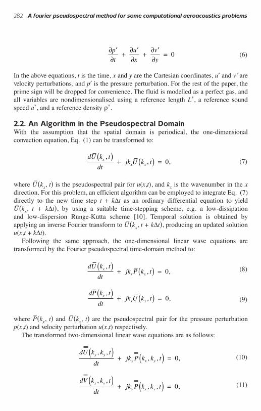
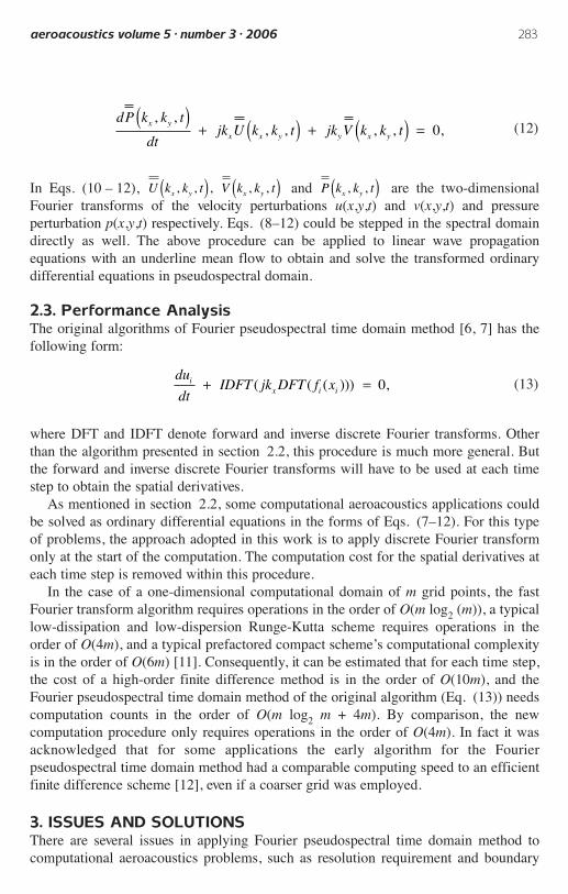
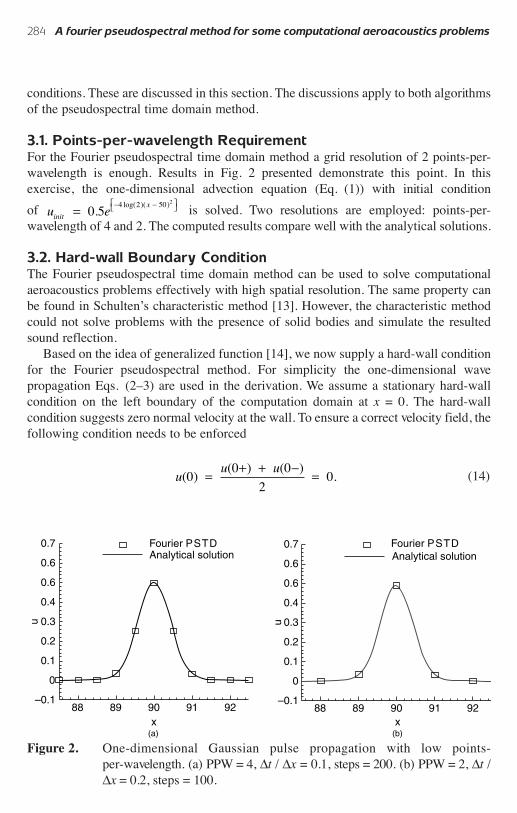
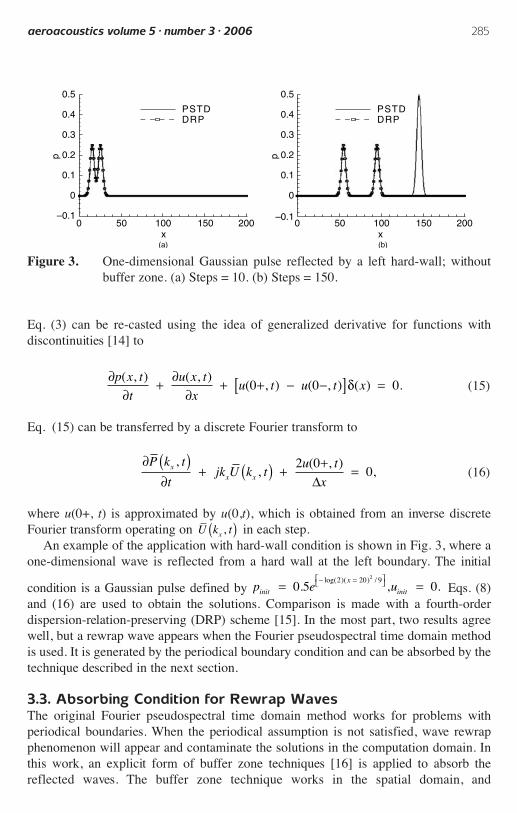
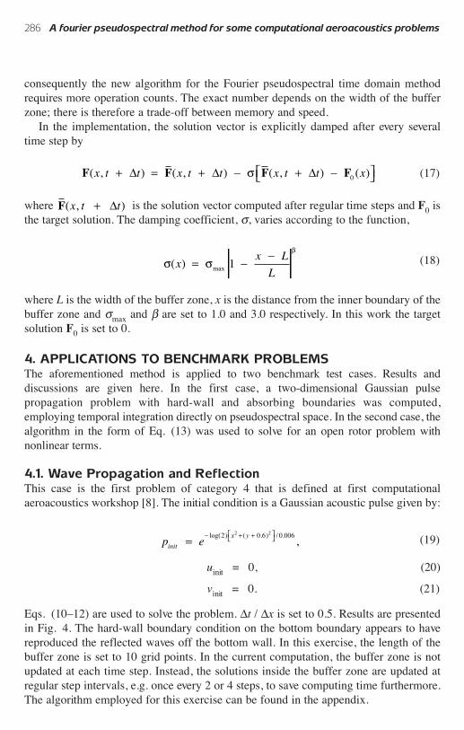
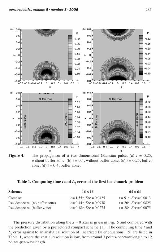
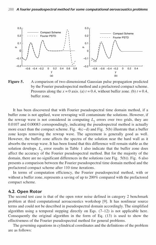
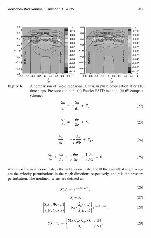
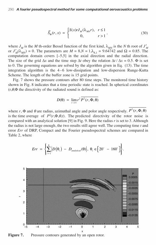
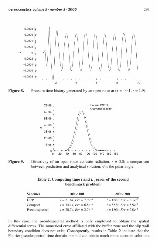
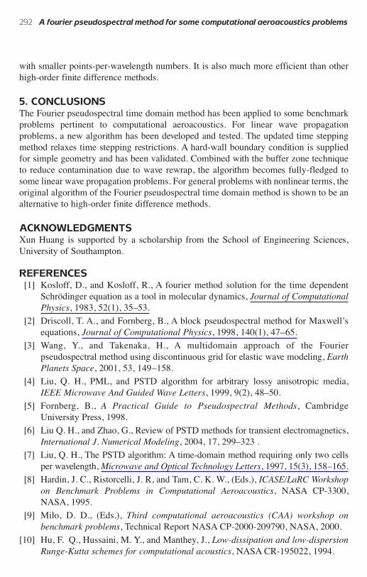
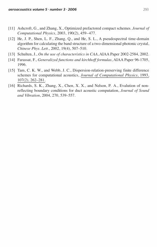
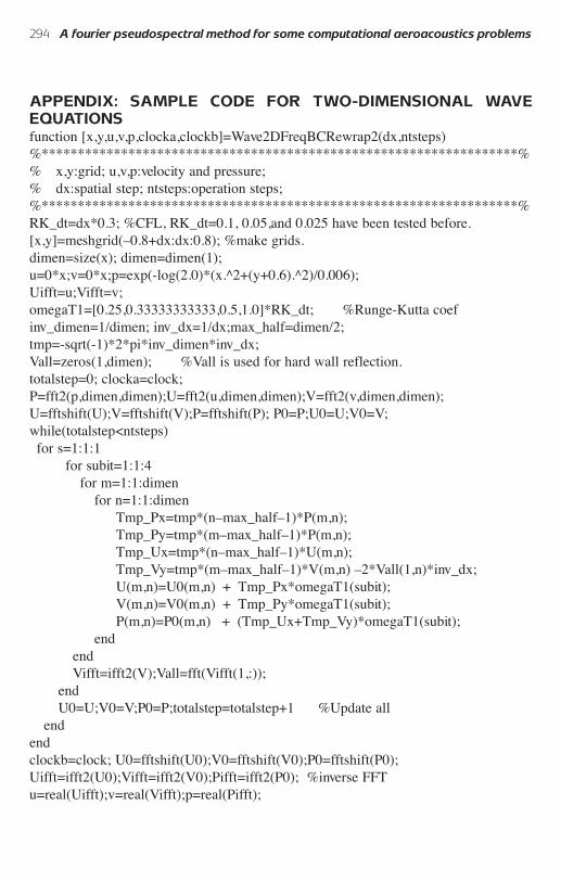


![Fourier Pseudospectral Solution for a 2D Nonlinear …[16], Bose-Einstein condensates 17], and plasma physics [ 18][, therefore in the present article we apply a Fourier pseudospectral](https://img.pdfslide.net/doc/110x75/5f2b2a6e18f6f1665861348e/fourier-pseudospectral-solution-for-a-2d-nonlinear-16-bose-einstein-condensates.jpg)