1

VKI Lecture Series:Advances in Aeroacoustics

Fundamentals of Aeroacoustics I

Sheryl GraceBoston University

What is Aeroacoustics

Direct approach for analyzing aeroacoustic phenomenon

Integral methodsFree-space Green’s functionMonopole, dipole, quadrupoleLighthill’s analogy

Extensions of the analogyFfowcs-Williams and Hawkings Eq./Curle’s eq.Kirchhoff methodHowe’s analogy

Acoustically compact sources

Outline

2

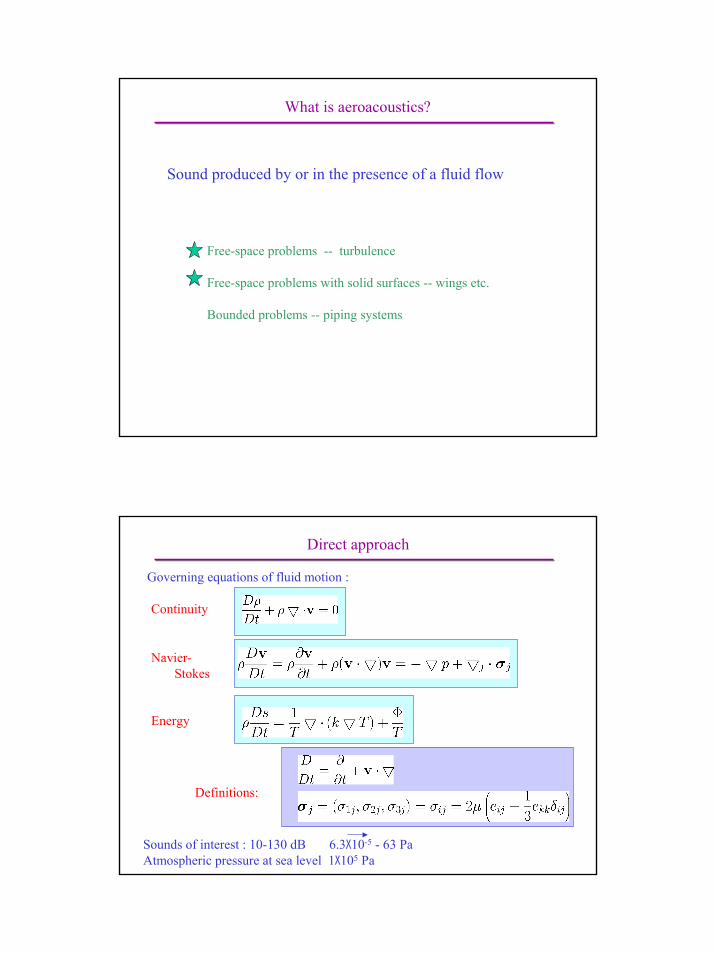
Sound produced by or in the presence of a fluid flow

What is aeroacoustics?

Free-space problems -- turbulence

Free-space problems with solid surfaces -- wings etc.

Bounded problems -- piping systems

Governing equations of fluid motion :

Direct approach

Continuity

Navier-Stokes

Definitions:

Sounds of interest : 10-130 dB 6.3X10-5 - 63 PaAtmospheric pressure at sea level 1X105 Pa

Energy

3

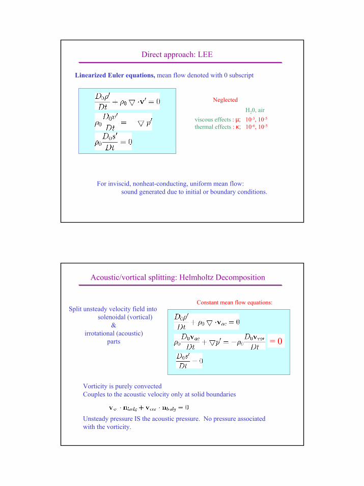
Linearized Euler equations, mean flow denoted with 0 subscript

Direct approach: LEE

H20, airviscous effects : µ; 10-3, 10-5

thermal effects : κ; 10-6, 10-5

Neglected

For inviscid, nonheat-conducting, uniform mean flow: sound generated due to initial or boundary conditions.

Split unsteady velocity field into solenoidal (vortical)

&irrotational (acoustic)

parts

Acoustic/vortical splitting: Helmholtz Decomposition

Constant mean flow equations:

Vorticity is purely convectedCouples to the acoustic velocity only at solid boundaries

= 0

Unsteady pressure IS the acoustic pressure. No pressure associatedwith the vorticity.

4

• Method has been used to compute interaction soundsee notes for references

• Popular applications: airfoil/gust, cascade/gust

Acoustic/vortical splitting: Comments

Vortical, acoustic, and entropic waves are decoupled in this approachNOT true when shocks occur or in swirling flow settings

Acoustic pressure associated with the irrotational portion of the flow which is driven by a coupling to the vortical and entropic portions of the field at solid surfaces.

Thus: VORTEX sound is a topic of great interest

Integral Methods

5

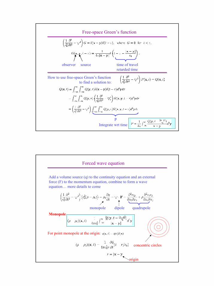
Free-space Green’s function

observer source time of travelretarded time

How to use free-space Green’s function to find a solution to:

PIntegrate wrt time

Forced wave equation

Add a volume source (q) to the continuity equation and an external force (F) to the momentum equation, combine to form a wave equation… more details to come

quadrupoledipolemonopoleMonopole

For point monopole at the origin:

origin

concentric circles

6

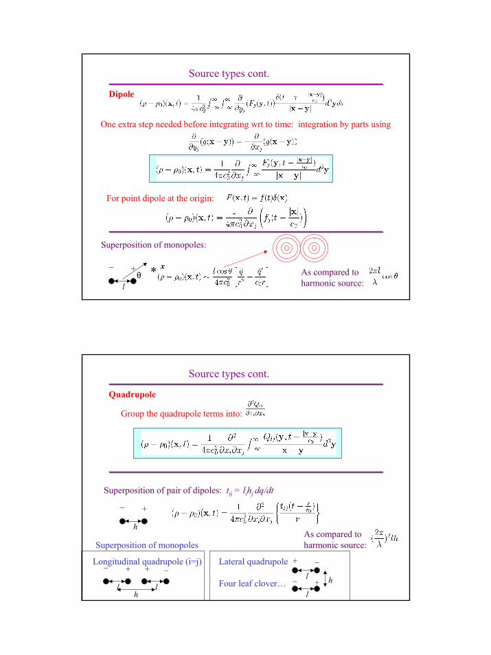
Source types cont.

Dipole

One extra step needed before integrating wrt to time: integration by parts using

Superposition of monopoles:

For point dipole at the origin:

x*+_

lθ As compared to

harmonic source:

Source types cont.

Quadrupole

Group the quadrupole terms into:

Superposition of pair of dipoles: tij = lihj dq/dt

+_

hAs compared to harmonic source:Superposition of monopoles

_+

l

+_

l

Longitudinal quadrupole (i=j) Lateral quadrupole

Four leaf clover… +_

l

_+

l h

h

7

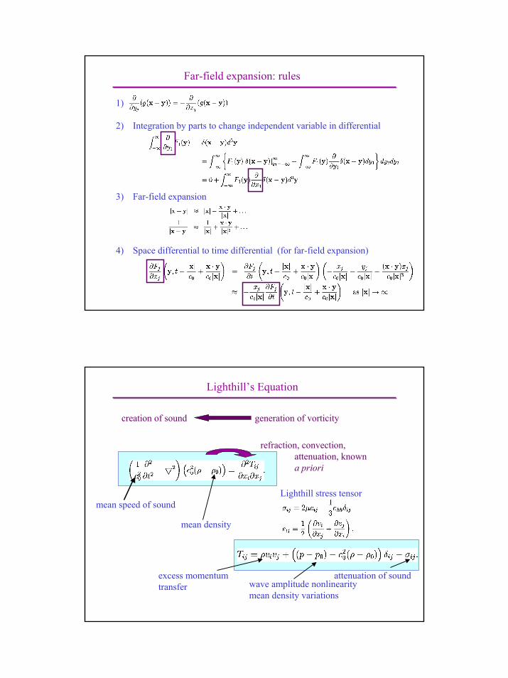
Far-field expansion: rules

Integration by parts to change independent variable in differential

1)

2)

3) Far-field expansion

4) Space differential to time differential (for far-field expansion)

Lighthill’s Equation

mean speed of soundLighthill stress tensor

mean density

creation of sound generation of vorticity

refraction, convection, attenuation, knowna priori

excess momentum transfer wave amplitude nonlinearity

mean density variations

attenuation of sound

8

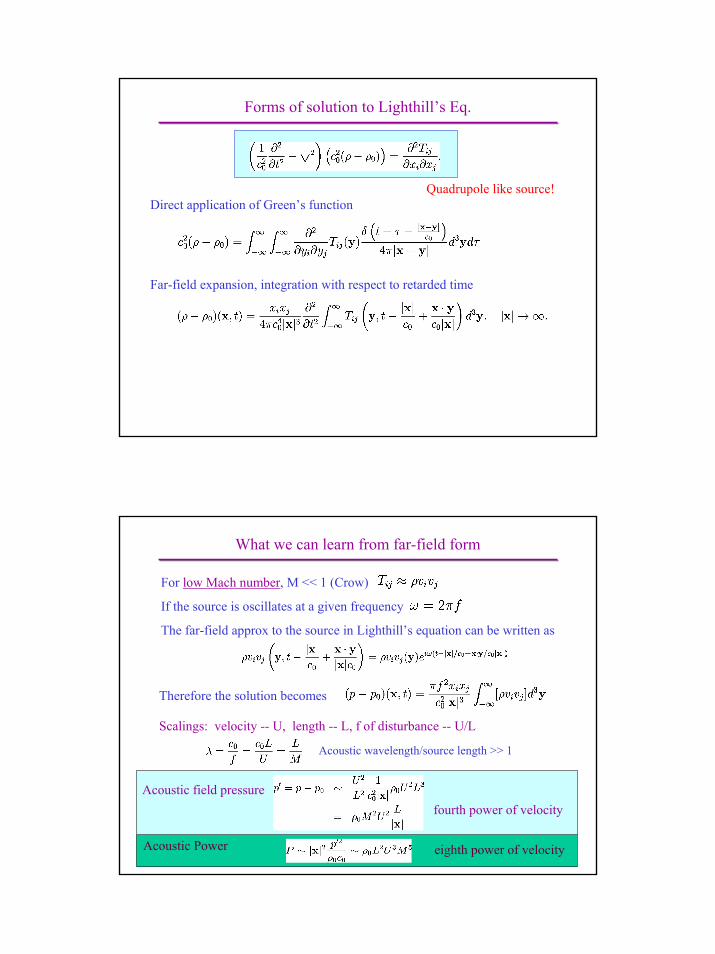
Forms of solution to Lighthill’s Eq.

Direct application of Green’s function

Far-field expansion, integration with respect to retarded time

Quadrupole like source!

What we can learn from far-field form

For low Mach number, M << 1 (Crow)

If the source is oscillates at a given frequency

The far-field approx to the source in Lighthill’s equation can be written as

Therefore the solution becomes

Scalings: velocity -- U, length -- L, f of disturbance -- U/L

Acoustic field pressure

Acoustic Power

fourth power of velocity

eighth power of velocity

Acoustic wavelength/source length >> 1

9

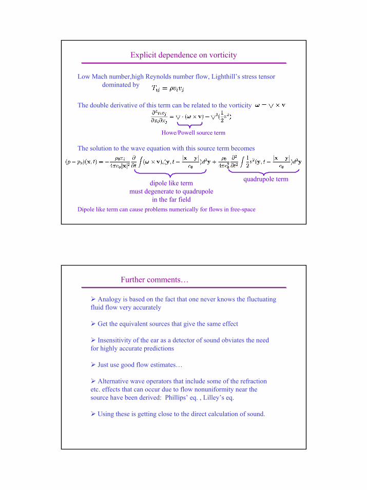
Explicit dependence on vorticity

Low Mach number,high Reynolds number flow, Lighthill’s stress tensor dominated by

The double derivative of this term can be related to the vorticity

The solution to the wave equation with this source term becomes

dipole like termmust degenerate to quadrupole

in the far field

quadrupole term

Dipole like term can cause problems numerically for flows in free-space

Howe/Powell source term

Further comments…

Analogy is based on the fact that one never knows the fluctuating fluid flow very accurately

Get the equivalent sources that give the same effect

Insensitivity of the ear as a detector of sound obviates the need for highly accurate predictions

Just use good flow estimates…

Alternative wave operators that include some of the refraction etc. effects that can occur due to flow nonuniformity near the source have been derived: Phillips’ eq. , Lilley’s eq.

Using these is getting close to the direct calculation of sound.

10

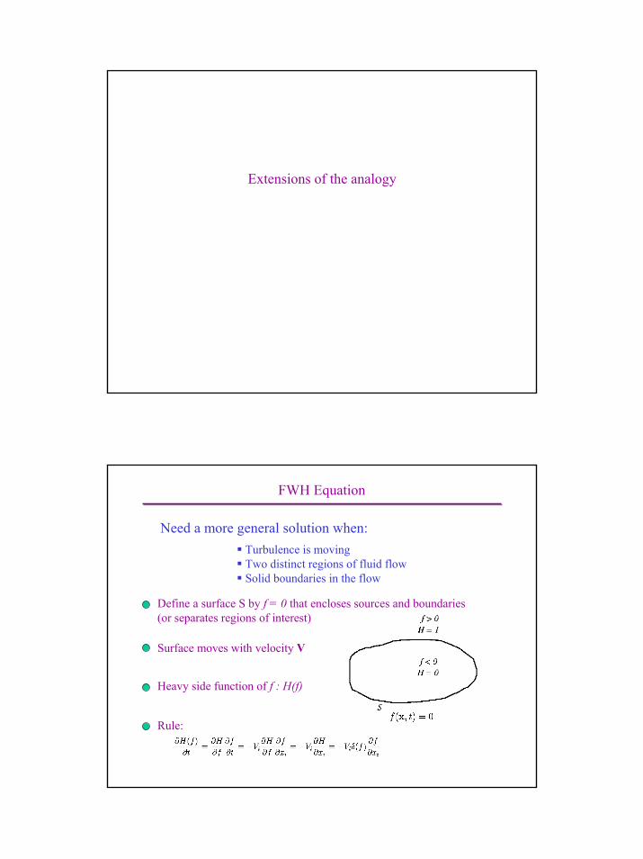
Extensions of the analogy

FWH Equation

Turbulence is moving Two distinct regions of fluid flowSolid boundaries in the flow

Need a more general solution when:

Define a surface S by f = 0 that encloses sources and boundaries (or separates regions of interest)

Surface moves with velocity V

Heavy side function of f : H(f)

Rule:

11

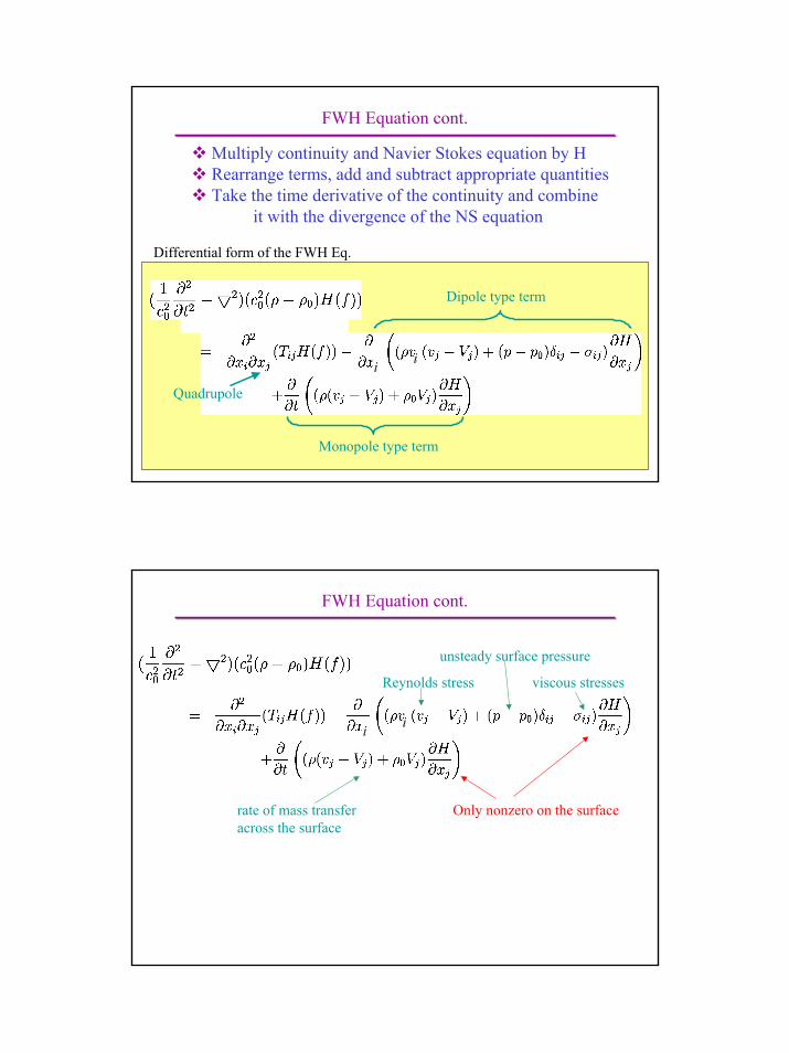
FWH Equation cont.

Multiply continuity and Navier Stokes equation by HRearrange terms, add and subtract appropriate quantitiesTake the time derivative of the continuity and combine

it with the divergence of the NS equation

Dipole type term

Monopole type term

Quadrupole

Differential form of the FWH Eq.

i i

Only nonzero on the surface

i i

FWH Equation cont.

Reynolds stress

unsteady surface pressure

viscous stresses

rate of mass transfer across the surface

12

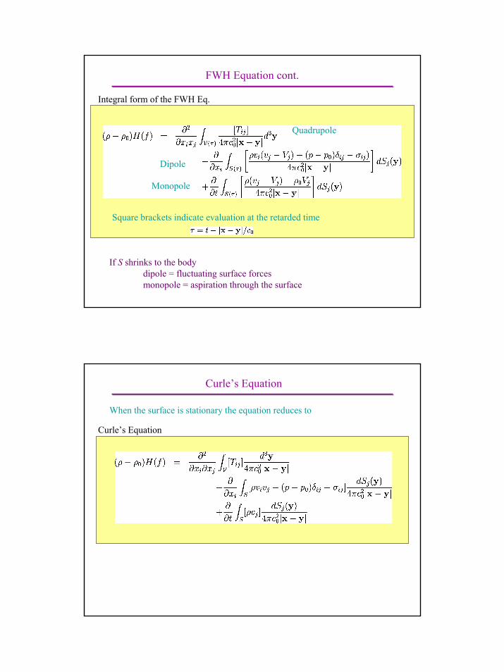
FWH Equation cont.

Dipole

Monopole

Quadrupole

Integral form of the FWH Eq.

Square brackets indicate evaluation at the retarded time

If S shrinks to the body dipole = fluctuating surface forcesmonopole = aspiration through the surface

Curle’s Equation

When the surface is stationary the equation reduces to

Curle’s Equation

13

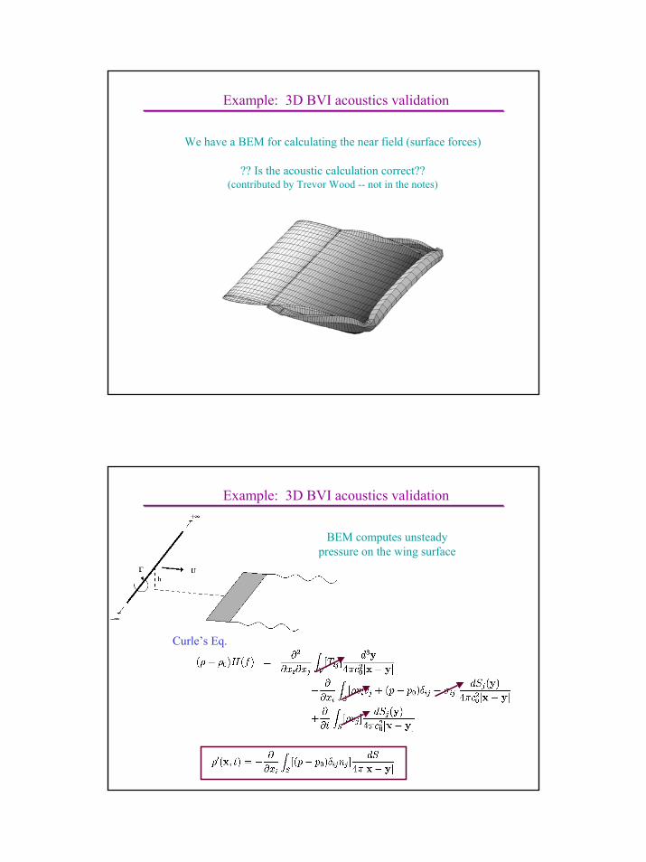
Example: 3D BVI acoustics validation

We have a BEM for calculating the near field (surface forces)

?? Is the acoustic calculation correct??(contributed by Trevor Wood -- not in the notes)

Example: 3D BVI acoustics validation

Curle’s Eq.

BEM computes unsteadypressure on the wing surface

14

Example: 3D BVI acoustics validation (cont.)

far-field expansion

integration of pressure is lift

interchange space and time derivatives

Acoustic pressure in non-dimensional form

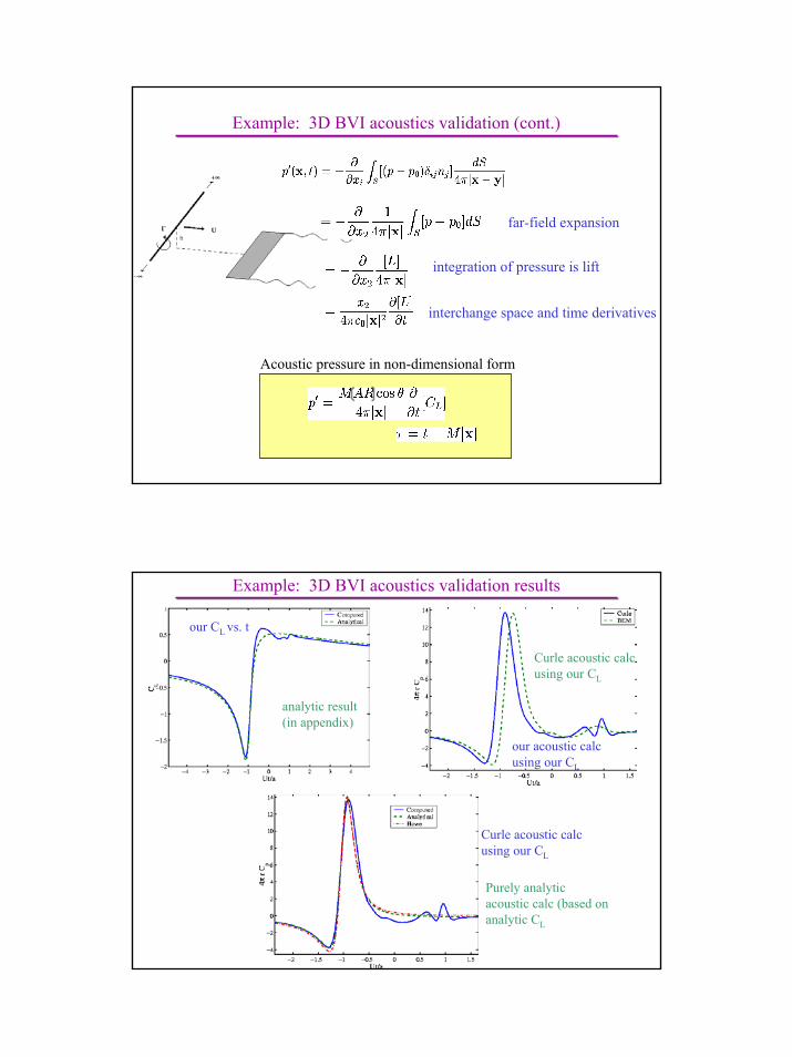
Example: 3D BVI acoustics validation results

our CL vs. t

analytic result(in appendix)

our acoustic calcusing our CL

Curle acoustic calcusing our CL

Curle acoustic calcusing our CL

Purely analytic acoustic calc (based on analytic CL

15

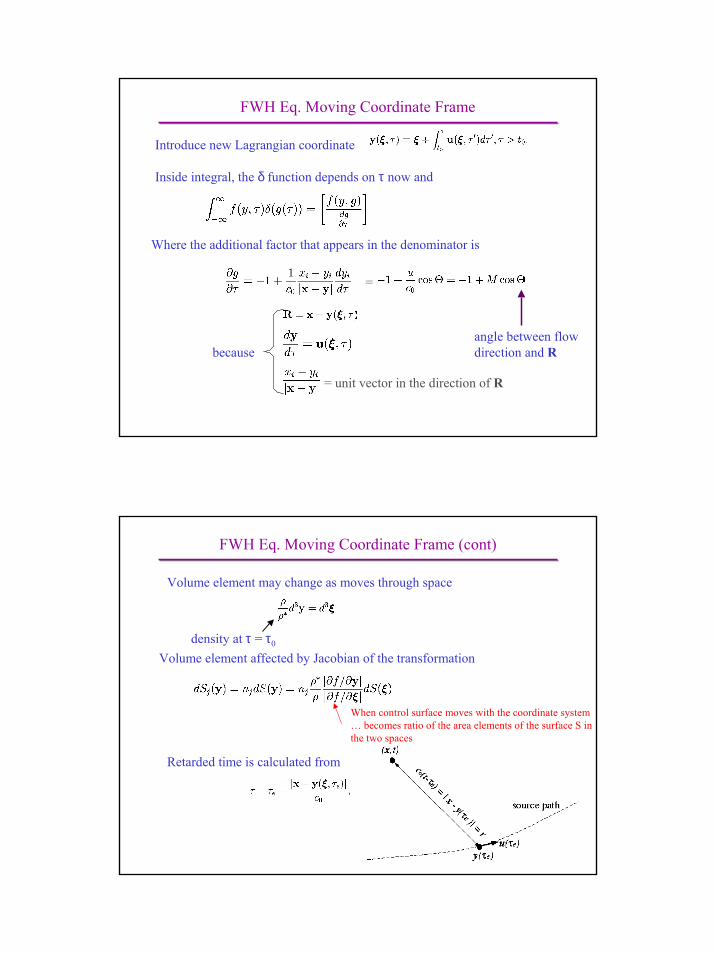
FWH Eq. Moving Coordinate Frame

Introduce new Lagrangian coordinate

Inside integral, the δ function depends on τ now and

Where the additional factor that appears in the denominator is

=

= unit vector in the direction of R

becauseangle between flow direction and R

FWH Eq. Moving Coordinate Frame (cont)

Volume element may change as moves through space

density at τ = τ0

Volume element affected by Jacobian of the transformation

Retarded time is calculated from

When control surface moves with the coordinate system … becomes ratio of the area elements of the surface S in the two spaces

16

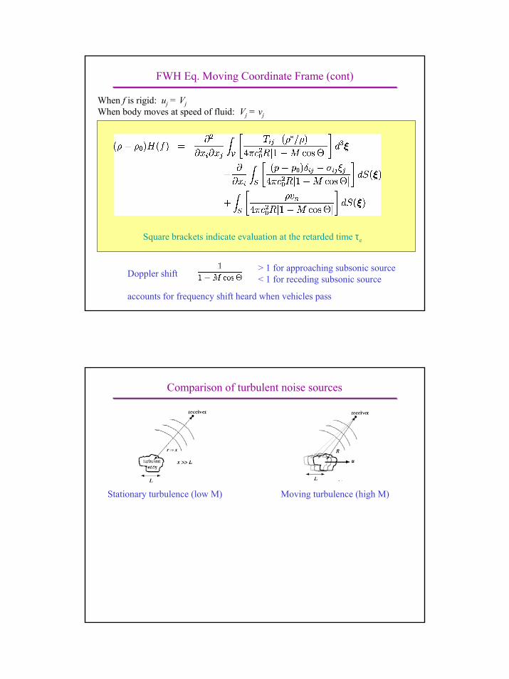
FWH Eq. Moving Coordinate Frame (cont)

When f is rigid: uj = VjWhen body moves at speed of fluid: Vj = vj

Square brackets indicate evaluation at the retarded time τe

Doppler shift

accounts for frequency shift heard when vehicles pass

> 1 for approaching subsonic source< 1 for receding subsonic source

Comparison of turbulent noise sources

Stationary turbulence (low M) Moving turbulence (high M)

17

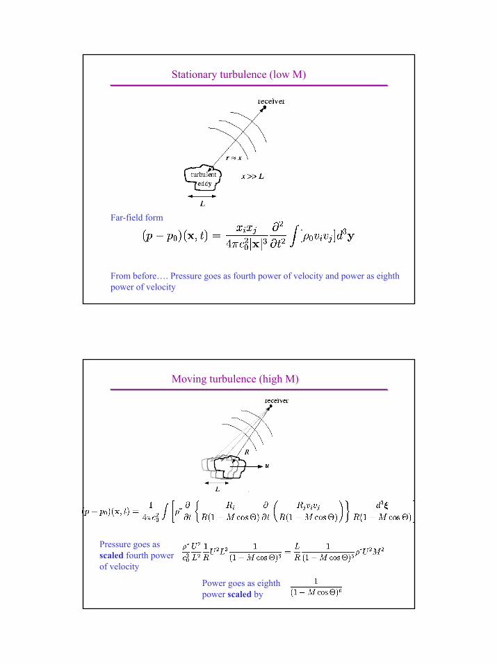
Stationary turbulence (low M)

Far-field form

From before…. Pressure goes as fourth power of velocity and power as eighth power of velocity

Moving turbulence (high M)

Pressure goes as scaled fourth power of velocity

Power goes as eighth power scaled by

18

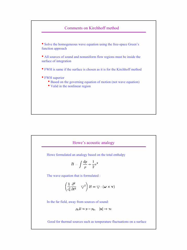
Comments on Kirchhoff method

• Solve the homogeneous wave equation using the free-space Green’s function approach

• All sources of sound and nonuniform flow regions must be inside the surface of integration

• FWH is same if the surface is chosen as it is for the Kirchhoff method

• FWH superior• Based on the governing equation of motion (not wave equation)• Valid in the nonlinear region

Howe’s acoustic analogy

Howe formulated an analogy based on the total enthalpy

The wave equation that is formulated :

In the far field, away from sources of sound:

Good for thermal sources such as temperature fluctuations on a surface

19

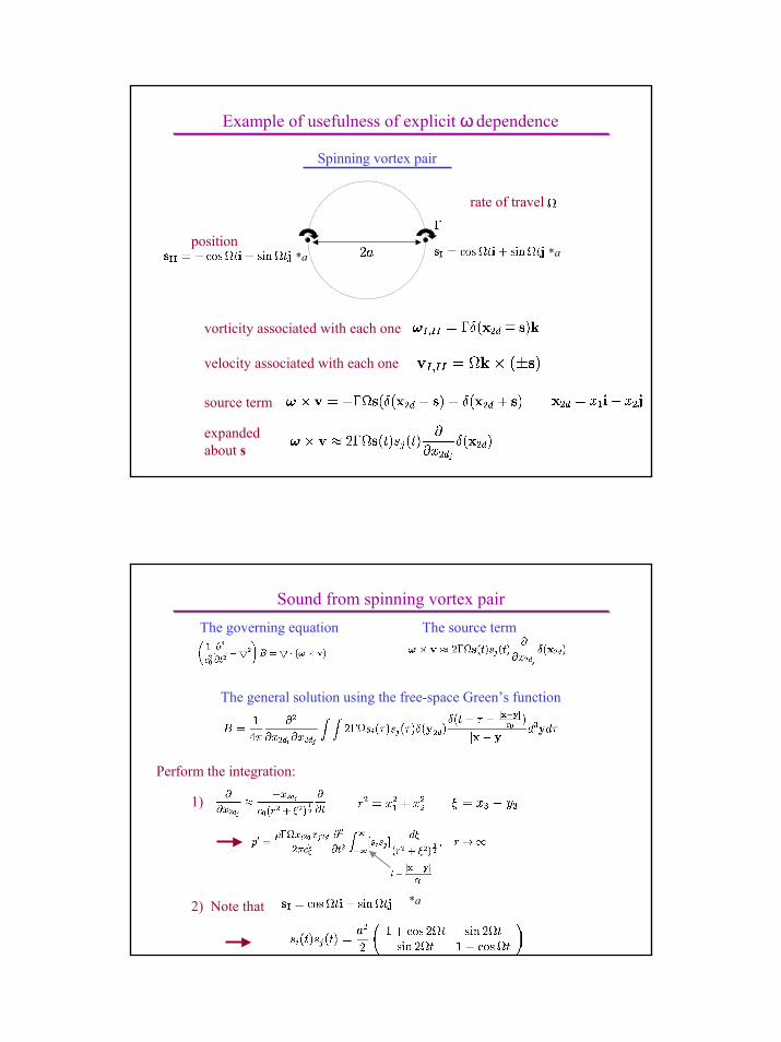
Example of usefulness of explicit ω dependence

Spinning vortex pair

rate of travel

position

vorticity associated with each one

velocity associated with each one

source term

expanded about s

*a*a

Sound from spinning vortex pairThe governing equation The source term

The general solution using the free-space Green’s function

Perform the integration:

1)

2) Note that *a

20

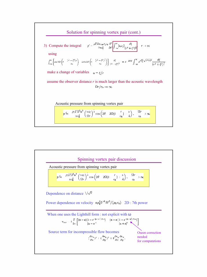
Solution for spinning vortex pair (cont.)

3) Compute the integral

using

make a change of variables

assume the observer distance r is much larger than the acoustic wavelength

Acoustic pressure from spinning vortex pair

Acoustic pressure from spinning vortex pair

Spinning vortex pair discussion

Dependence on distance

Power dependence on velocity 2D : 7th power

When one uses the Lighthill form : not explicit with ω

Source term for incompressible flow becomes Oseen correctionneeded for computations

21

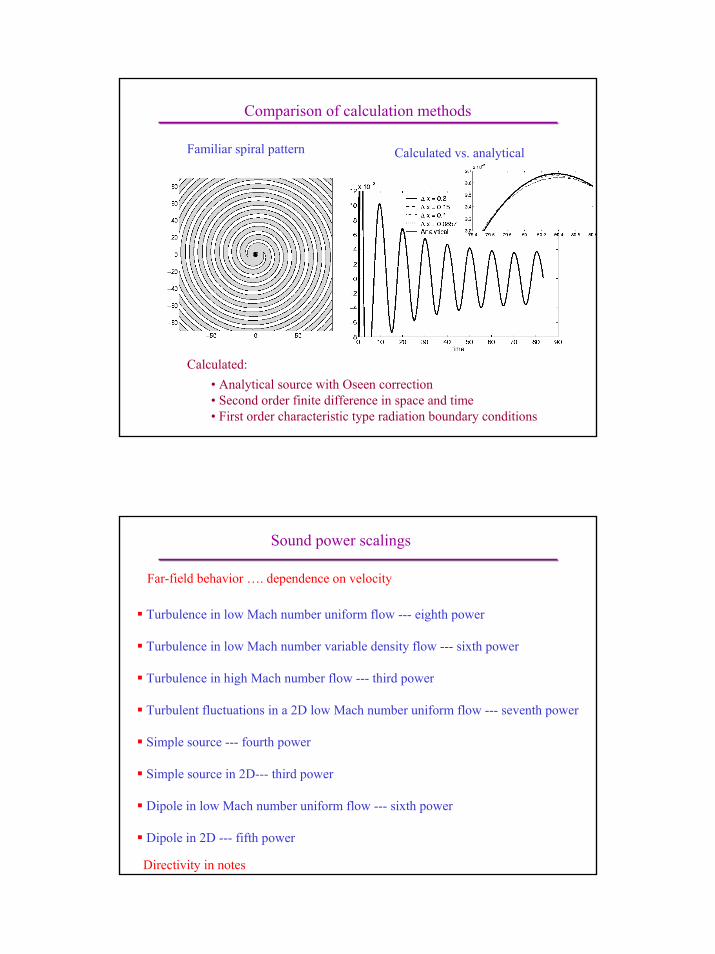
Comparison of calculation methods

Familiar spiral pattern Calculated vs. analytical

• Analytical source with Oseen correction• Second order finite difference in space and time• First order characteristic type radiation boundary conditions

Calculated:

Sound power scalings

Far-field behavior …. dependence on velocity

Turbulence in low Mach number uniform flow --- eighth power

Turbulence in low Mach number variable density flow --- sixth power

Turbulence in high Mach number flow --- third power

Turbulent fluctuations in a 2D low Mach number uniform flow --- seventh power

Simple source --- fourth power

Simple source in 2D--- third power

Dipole in low Mach number uniform flow --- sixth power

Dipole in 2D --- fifth power

Directivity in notes

22

Acoustically compact source

Alternative method of defining integral form of wave eq.

Meaning of compact

Given:Characteristic length scale of the source region : LWavelength of the sound : λ

If :L/λ << 1 we say that the source region is acoustically compact

23

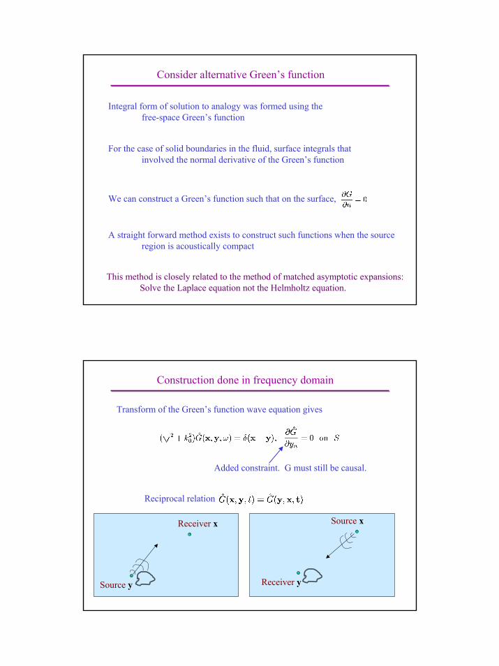
Consider alternative Green’s function

Integral form of solution to analogy was formed using the free-space Green’s function

For the case of solid boundaries in the fluid, surface integrals thatinvolved the normal derivative of the Green’s function

A straight forward method exists to construct such functions when the sourceregion is acoustically compact

We can construct a Green’s function such that on the surface,

This method is closely related to the method of matched asymptotic expansions:Solve the Laplace equation not the Helmholtz equation.

Construction done in frequency domain

Transform of the Green’s function wave equation gives

Added constraint. G must still be causal.

Reciprocal relation

Source y

Receiver x Source x

Receiver y

24

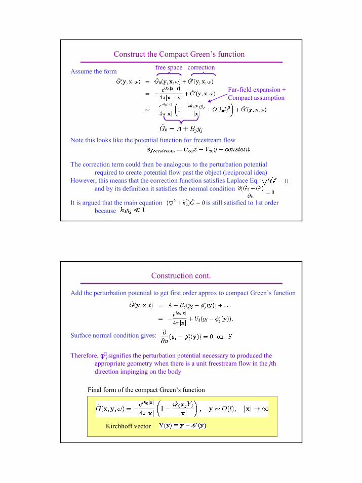
It is argued that the main equation is still satisfied to 1st orderbecause

The correction term could then be analogous to the perturbation potentialrequired to create potential flow past the object (reciprocal idea)

However, this means that the correction function satisfies Laplace Eq. and by its definition it satisfies the normal condition

Construct the Compact Green’s function

Assume the form free space correction

Note this looks like the potential function for freestream flow

Far-field expansion +Compact assumption

Construction cont.

Add the perturbation potential to get first order approx to compact Green’s function

Surface normal condition gives:

Therefore, φ∗j signifies the perturbation potential necessary to produced the

appropriate geometry when there is a unit freestream flow in the jthdirection impinging on the body

Final form of the compact Green’s function

Kirchhoff vector

25

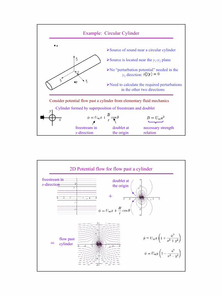
Example: Circular Cylinder

Source of sound near a circular cylinder

Source is located near the y1-y2 plane

No “perturbation potential” needed in the y3 direction:

Need to calculate the required perturbationsin the other two directions

Consider potential flow past a cylinder from elementary fluid mechanics

Cylinder formed by superposition of freestream and doublet

freestream in x-direction

x

y

doublet at the origin

necessary strengthrelation

2D Potential flow for flow past a cylinder

freestream in x-direction

doublet at the origin

+

=flow pastcylinder

26

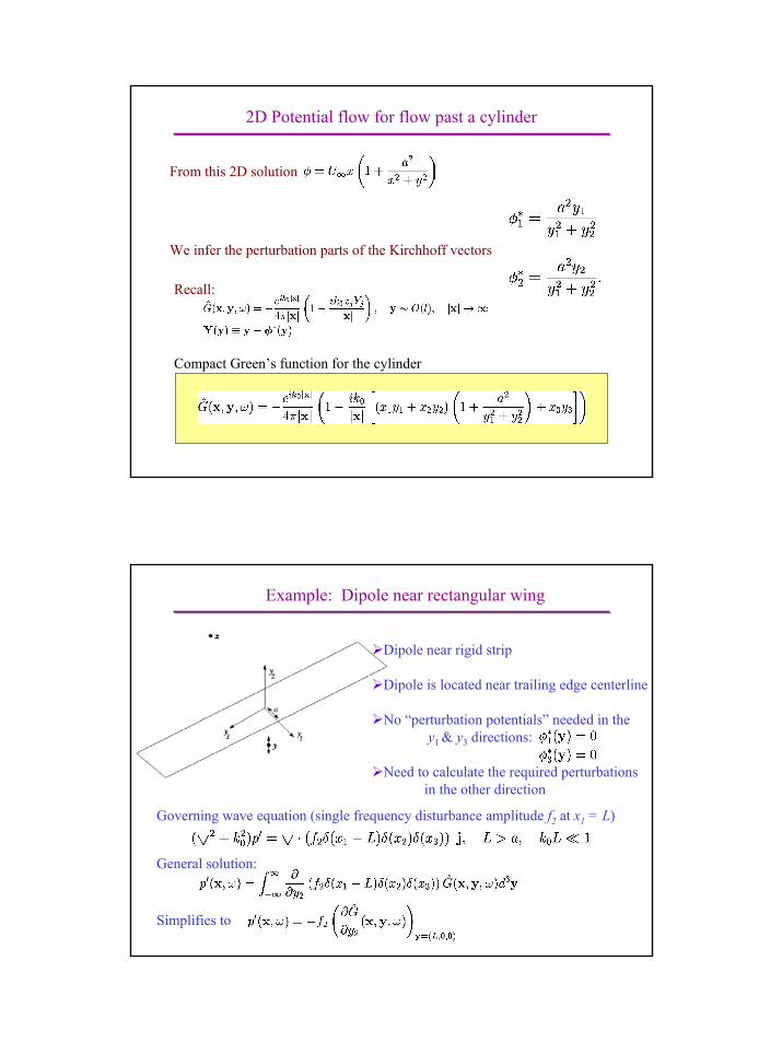
2D Potential flow for flow past a cylinder

From this 2D solution

We infer the perturbation parts of the Kirchhoff vectors

Compact Green’s function for the cylinder

Recall:

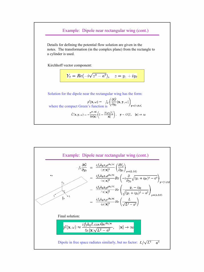
Example: Dipole near rectangular wing

Dipole near rigid strip

Dipole is located near trailing edge centerline

No “perturbation potentials” needed in the y1 & y3 directions:

Need to calculate the required perturbationsin the other direction

Governing wave equation (single frequency disturbance amplitude f2 at x1 = L)

General solution:

Simplifies to

27

Solution for the dipole near the rectangular wing has the form:

Kirchhoff vector component:

where the compact Green’s function is

Details for defining the potential flow solution are given in thenotes. The transformation (in the complex plane) from the rectangle to a cylinder is used.

Example: Dipole near rectangular wing (cont.)

Example: Dipole near rectangular wing (cont.)

Final solution:

Dipole in free space radiates similarly, but no factor:

28

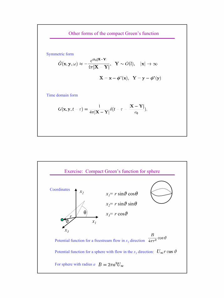
Other forms of the compact Green’s function

Symmetric form

Time domain form

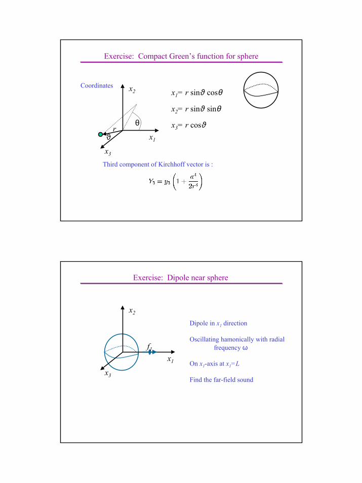
Exercise: Compact Green’s function for sphere

x1

x2

x3

ϑ

θ

x1= r sinϑ cosθ

r

x2= r sinϑ sinθ

x3= r cosϑ

Potential function for a sphere with flow in the x3 direction:

For sphere with radius a

Potential function for a freestream flow in x3 direction

Coordinates

29

x1

x2

x3

ϑ

θ

x1= r sinϑ cosθ

r

x2= r sinϑ sinθ

x3= r cosϑ

Exercise: Compact Green’s function for sphere

Third component of Kirchhoff vector is :

Coordinates

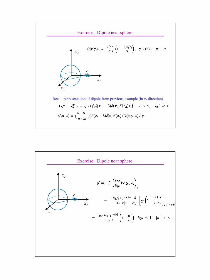
Exercise: Dipole near sphere

x1

x2

x3

f1

Dipole in x1 direction

Oscillating hamonically with radialfrequency ω

On x1-axis at x1=L

Find the far-field sound

30

Exercise: Dipole near sphere

x1

x2

x3

f1

Recall representation of dipole from previous example (in x2 direction)

x1

Exercise: Dipole near sphere

x1

x2

x3

f1

31