AIAA JOURNALVol. 33, No. 10, October 1995

Computational Aeroacoustics: Issues and Methods

Christopher K. W. Tarn*Florida State University, Tallahassee, Florida 32306-3027

Computational fluid dynamics (CFD) has made tremendous progress especially in aerodynamics and aircraftdesign over the past 20 years. An obvious question to ask is "why not use CFD methods to solve aeroacousticsproblems?" Most aerodynamics problems are time independent, whereas aeroacoustics problems are, by definition,time dependent. The nature, characteristics, and objectives of aeroacoustics problems are also quite different fromthe commonly encountered CFD problems. There are computational issues that are unique to aeroacoustics.For these reasons computational aeroacoustics requires somewhat independent thinking and development. Theobjectives of this paper are twofold. First, issues pertinent to aeroacoustics that may or may not be relevant tocomputational aerodynamics are discussed. The second objective is to review computational methods developedrecently that are designed especially for computational aeroacoustics applications. Some of the computationalmethods to be reviewed are quite different from traditional CFD methods. They should be of interest to the CFDand fluid dynamics communities.

Nomenclature#0 = speed of soundD = jet diameter at nozzle exiter = unit vector in the r directionee = unit vector in the 9 direction/ = frequencyL = core length of a jetp = pressureu = velocity componentUj = jet exit velocitya = wave numbera = wave number of a finite difference schemeP = wave number in the y directionA£ = time stepAJC = size of spatial mesh8 = thickness of mixing layerX = acoustic wave lengthva = artificial kinematic viscosityp = densityco = angular frequencya) = angular frequency of a finite difference schemeo)i = imaginary part of the angular frequency

I. Introduction

I T is no exaggeration to say that computational fluid dynamics(CFD) has made impressive progress during the last 20 years,

especially in aerodynamics computation. In the hands of competentengineers, CFD has become not only an indispensable method foraircraft load prediction but also a reliable design tool. It is incon-ceivable that future aircraft would be designed without CFD.

Needless to say, CFD methods have been very successful forthe class of problems for which they were invented. An obviousquestion to ask is "why not use CFD methods to solve aeroacous-tics problems?" To answer this question, one must recognize thatthe nature, characteristics, and objectives of aeroacoustics prob-lems are distinctly different from those commonly encountered inaerodynamics. Aerodynamics problems are, generally, time inde-pendent, whereas aeroacoustics problems are, by definition, time

Received Nov. 1, 1994; presented as Paper 95-0677 at the AIAA 33rdAerospace Sciences Meeting, Reno, NV, Jan. 9-12,1995; revision receivedMarch 13, 1995; accepted for publication March 15, 1995. Copyright ©1995 by Christopher K. W. Tarn. Published by the American Institute ofAeronautics and Astronautics, Inc., with permission.

* Professor, Department of Mathematics. Associate Fellow AIAA.

dependent. In most aircraft noise problems, the frequencies are veryhigh. Because of these reasons, there are computational issues thatare relevant and unique to aeroacoustics. To resolve these issues,computational aeroacoustics (CAA) requires independent thinkingand development.

An important point needs to be made at this stage. Computationalaeroacoustics is not computational methods alone. If so, it wouldbe called computational mathematics. The application of compu-tational methods to aeroacoustics problems for the purpose of un-derstanding the physics of noise generation and propagation, or forcommunity noise prediction and aircraft certification, is the mostimportant part of CAA. The problem area may be in jet noise, air-frame noise, fan and turbomachinery noise, propeller and helicopternoise, duct acoustics, interior noise, sonic boom, or other subfieldsof aeroacoustics (see Ref. 1 for details). Computational methods arethe tools but not the ends of CAA. It is aeroacoustics that definesthe area.

As yet there has not been widespread use of computational meth-ods for solving aeroacoustics problems. This paper, therefore, con-centrates on discussing the methodology issues in CAA in the hopeof stimulating interest in CAA applications and further develop-ments or improvements of computational methods.

The first objective of this paper is to discuss issues pertinent toaeroacoustics that may or may not be relevant to computationalaerodynamics. To provide a concrete illustration of these issues,the case of direct numerical simulation of supersonic jet flows andnoise radiation will be used. The second objective is to review re-cently developed computational methods designed especially forCAA applications.

Before one designs a computational algorithm for simulatingsupersonic jet noise generation and radiation, it is important thatone has some idea of the physics of supersonic jet noise. This isextremely important, for any computational scheme would have afinite resolution. This limitation prevents it from being capable ofresolving phenomena associated with finer scales of the problem.The principal components of supersonic jet noise are the turbu-lent mixing noise, the broadband shock-associated noise, and thescreech tones.2'3 In a supersonic jet, the turbulence in the jet flowcan be divided into the large-scale turbulence structures/instabilitywaves and the fine-scale turbulence. Both the large turbulence struc-tures and the fine-scale turbulence are noise sources. However, it isknown2-3 that for hot jets of Mach number 1.5 or higher the largeturbulence structures/instability waves are responsible for the gen-eration of the dominant part of all of the three principal componentsof supersonic jet noise. In the discussion that follows, it will beassumed that the noise from fine-scale turbulence, being less impor-tant, is ignored. The resolution of fine-scale turbulence is, therefore,not a primary issue.

1788

TAM 1789

II. Issues Relevant to CAATo illustrate the various computational issues relevant to CAA,

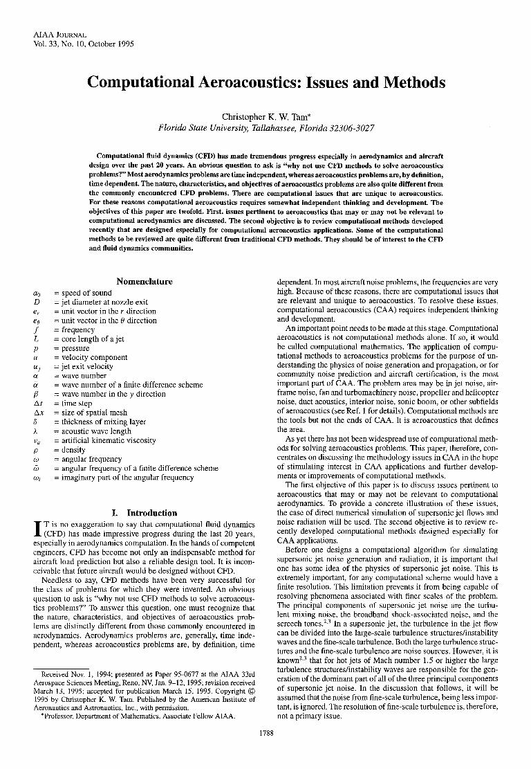
we will consider the case of direct numerical simulation of the gen-eration and radiation of supersonic jet noise by the large turbulencestructures/instability waves of the jet flow. Since a computation do-main must be finite, it appears that a good choice is to select adomain nearly identical to that in a physical experiment. Figure 1shows a schematic diagram of a supersonic jet noise experiment in-side an anechoic chamber. The exit diameter of the nozzle is a naturallength scale of the problem. In order that microphone measurementsdo provide representative far-field noise data, the lateral wall of theanechoic chamber should be placed not less than 40 diameters fromthe jet axis. For a high-speed supersonic jet, the centerline jet veloc-ity in the fully developed region of the jet decays fairly slowly, i.e.,inversely proportional to the downstream distance. Thus, even at adownstream distance of 50 jet diameters, the jet velocity would stillbe in the moderately subsonic Mach number range. To avoid strongoutflow velocity and to contain all of the noise-producing regionof the jet inside the anechoic chamber, it is preferable to have thewall where the diffuser is located to be at least 60 diameters down-stream from the nozzle exit. The preceding considerations definethe minimum size of the anechoic chamber that will be used as thecomputational domain.

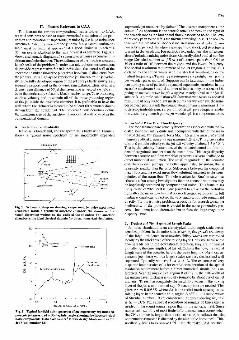
A. Large Spectral BandwidthJet noise is broadband, and the spectrum is fairly wide. Figure 2

shows a typical noise spectrum of an imperfectly expanded

entrainment flowX

Fig. 1 Schematic diagram showing a supersonic jet noise experimentconducted inside a ventilated anechoic chamber. Not shown are thesound-absorbing wedges on the walls of the chamber. The anechoicchamber is the ideal physical domain for direct numerical simulation.

130

110

90

70

50

screech tone

0.03 0.1 1Strouhal number, St = fD/Uj

Fig. 2 Typical far-field noise spectrum of an imperfectly expanded su-personic jet, measured at 30-deg inlet angle, showing the three principalnoise components. Data from Seiner.4 Nozzle design Mach number 2.0.Jet Mach number 1.5.

supersonic jet measured by Seiner.4 The discrete component at thecenter of the spectrum is the screech tone. The peak to the right ofthe screech tone is the broadband shock-associated noise. The low-frequency peak to the left is the turbulent mixing noise. The screechtone and the broadband shock-associated noise exist only for im-perfectly expanded jets when a quasiperiodic shock cell structure ispresent in the jet plume. For perfectly expanded jets, the noise con-sists of turbulent mixing noise alone. Generally, the Strouhal numberrange (Strouhal number = fD/Uj) of interest spans from 0.01 to10 or a ratio of 103 between the highest and the lowest frequency.The spatial resolution requirement of the jet (region A of Fig. 1) isdictated by the sound waves with the shortest wavelengths or thehighest frequencies. Typically a minimum of six to eight mesh pointsper wavelength is required. Suppose one is interested in the turbu-lent mixing noise of perfectly expanded supersonic jets alone. In thiscase, the maximum Strouhal number of interest may be taken as 1.0,giving an acoustic wave length A approximately equal to the jet di-ameter D. A simple calculation will show that even by using a spatialresolution of only six to eight mesh points per wavelength, the num-ber of mesh points inside the computation domain is enormous. Howto develop finite difference algorithms that will give adequate resolu-tion at six to eight mesh points per wavelength is an important issue.

B. Acoustic Wave/Mean Flow DisparityThe root-mean-square velocity fluctuation associated with the ra-

diated sound is usually quite small compared with that of the meanflow of the jet. For example, for a Mach 1.5 jet the measured soundintensity at 40 jet diameters away is around 124 dB. This gives a ratioof sound particle velocity to the jet exit velocity of about 1.5 x 10~4.That is, the velocity fluctuations of the radiated sound are four or-ders of magnitude smaller than the mean flow. This large disparitybetween acoustic and flow variables presents a severe challenge todirect numerical simulation. The small magnitude of the acousticdisturbances can, perhaps, be better appreciated by noting that itis usually smaller than the error (difference between the computedmean flow and the exact mean flow solution) incurred in the com-putation of the mean flow. This observation led Roe5 to state that"there is a fear among investigators that the acoustic solutions maybe hopelessly corrupted by computational noise." This issue raisesthe question of whether it is more prudent to solve for the perturba-tions after the mean flow has first been determined or to solve the fullnonlinear equations to capture the very small-amplitude sound fielddirectly. For the jet noise problem, especially for screech tones, thenonlinearity of the problem is crucial to the noise generation pro-cess. Thus, there is no alternative but to face the large-magnitudedisparity issue.

C. Distinct and Well-Separated Length ScalesJet noise simulation is an archetypical multilength scale aeroa-

coustics problem. In the noise source region, the growth and decayof the large turbulence structures/instability waves are controlledlocally by the thickness 8 of the mixing layer. However, because theflow spreads out in the downstream direction, they are influencedglobally by the core length L of the jet. Outside the flow, the naturallength scale of the acoustic field is the wave length A. For most su-personic jets, these various length scales are very distinct and wellseparated, typically we have 8 <^ X < L. The existence of verydisparate length scales calls for careful consideration of the spatialresolution requirement before a direct numerical simulation is at-tempted. Near the nozzle exit, region B of Fig. 1, the half-width ofthe mixing layer thickness is usually found to be about 5% of the jetdiameter. To resolve adequately the instability waves in the mixinglayer of the jet, a minimum of say 15 mesh points are needed. Thisgives Ar = 0.0033D where Ar is the radial mesh spacing in themixing layer. In the acoustic field, region A of Fig. 1, if sound wavesof Strouhal number 1.0 are considered, the mesh spacing requiredis Ar = D/6. Thus a spatial resolution of roughly 50 times finer isneeded in the sound source region than in the acoustic field. Sincenumerical instability of most finite difference schemes occurs whenfhe CFL number is larger than a critical value, it follows that thecomputation time step is dictated by the size of the finest mesh. This,needlessly, leads to excessive CPU time. To make CAA practical,

1790 TAM

methods that would overcome the curse of disparate length scalesare very much needed.

D. Long Propagation DistanceThe quantities of interest in aeroacoustics problems, invariably,

are the directivity and spectrum of the radiated sound in the farfield. Thus the computed solution must be accurate throughout theentire computation domain. This is in sharp contrast to aerodynam-ics problems where the primary interest is in determining the load-ing and moments acting on an airfoil or aerodynamic body. In thisclass of problems, a solution that is accurate only in the vicinityaround the airfoil or body would be sufficient. The solution doesnot need to be uniformly accurate throughout the entire compu-tation domain.

The distance from the noise source to the boundary of the com-putation domain is usually quite long. To ensure that the computedsolution is uniformly accurate over such long propagation distance,the numerical scheme must be almost free of numerical dispersion,dissipation, and anisotropy. If a large number of mesh points perwavelength are used, this is not difficult to accomplish. However,if one is restricted to the use of only six to eight mesh points perwavelength, the issue is nontrivial. To see the severity of the re-quirement, let us perform the following estimate for the jet noiseproblem. Numerical dispersion error is the result of the differencebetween the group velocities (not the phase velocity as commonlybelieved) of the waves associated with different wave numbers ofthe finite difference equations and that of the original partial dif-ferential equations. Assume that the computation boundary is at40 jet diameters away. Let a (a) be the wave number of the finitedifference scheme (see Sec. Ill or Ref. 6 for the definition of a).Then the group velocity of the acoustic waves of the numericalscheme is given by (da/da)a0 (assuming the numerical schemeis dispersion relation preserving). The time needed for the soundwave to propagate to the boundary of the computation domainis 40D/00- Thus, the displaced distance due to numerical disper-sion is [(da/da)ao — ao](40D/a0). If a mesh of six spacings perjet diameter is used and an accumulated numerical displacementless than one mesh spacing is desired, then the slope of the a (a)curve of the numerical scheme must satisfy the stringent require-ment of

daI

4 0 x 6 (1)

Most low-order finite difference schemes do not satisfy the preced-ing condition.

Finite difference schemes, invariably, have built-in numerical dis-sipation arising from time discretization. This causes a degradationof the computed sound amplitude. Suppose AdB is the acceptablenumerical error in decibels. Then, it is easy to show that if &>/ isthe imaginary part of the angular frequency of the numerical time-marching scheme, this condition can be expressed mathematically6

as

240 ' (2)

In the case of AdB = 1.0 and the Courant-Friedrichs-Lewy numberAtao/Ajc = 0.25, it is straightforward to find cot &t > —1.2 x10~4. Very few time-marching schemes can meet this demandingrequirement.

£. Radiation and Outflow Boundary ConditionsA computation domain is inevitably finite in size. Because of this,

radiation and outflow boundary conditions are required at its artifi-cial boundaries. These boundary conditions allow the acoustic andflow disturbances to leave the computation domain with minimalreflection. Again let us consider the problem of direct numericalsimulation of jet noise radiation from a supersonic jet as shown inFig. 1. The jet entrains a significant amount of ambient fluid so thatunless the computation domain is very large, there will be nonuni-form time-independent inflow at its boundaries. At the same time,the jet flow must leave the computation domain through some part

of its boundary. Along this part of the boundary, there is a steadyoutflow. It is well known that the Euler equations support three typesof small-amplitude disturbances. They are the acoustic, the vortic-ity, and entropy waves. Locally, the acoustic waves propagate at avelocity equal to the vector sum of the acoustic speed and the meanflow velocity. The vorticity and entropy waves, on the other hand,are convected downstream at the same speed and direction as themean flow. Thus, radiation boundary conditions are required alongboundaries with inflow to allow the acoustic waves to propagate outof the computation domain as in region C of Fig. 1. Along boundarieswith outflow such as region D of Fig. 1, a set of outflow boundaryconditions is required to facilitate the exit of the acoustic, vorticity,and entropy disturbances.

F. NonlinearitiesMost aeroacoustics problems are linear. The supersonic jet noise

problem is an exception. It is known experimentally when the jetis imperfectly expanded, strong screech tones are emitted by thejet. The intensity of screech tones around the jet can be as high as160 dB. At this high intensity, nonlinear distortion of the acousticwaveform is expected. However, because of the three-dimensionalspreading of the wave front, experimental measurements inside ane-choic chambers do not indicate the formation of shocks. Thus, inthe acoustic field, a shock-capturing scheme is not strictly required.

Although there are no acoustic shocks, inside the plume of an im-perfectly expanded jet, shocks and expansion fans are formed. Theseshocks are known to be responsible for the generation of screechtones and broadband shock noise.2'3 These shocks are highly un-steady. The use of a good shock-capturing scheme that does notgenerate spurious numerical waves by itself is, therefore, highlyrecommended in any direct numerical simulation of noise fromshock-containing jets.

G. Wall Boundary ConditionsThe imposition of wall boundary conditions are necessary when-

ever there are solid surfaces present in a flow or sound field. Accuratewall conditions are especially important for interior problems suchas duct acoustics and noise from turbomachinery. For the super-sonic jet noise problem, solid wall boundary conditions are neededto simulate the presence of the nozzle as shown in Fig. 1.

It is easy to see, unless all of the first-order spatial derivativesof the Euler equations are approximated by first-order finite differ-ences, the order of the resulting finite difference equations would behigher than the original partial differential equations. With higherorder governing equations, the number of boundary conditions re-quired for a unique solution is larger. In other words, by using ahigh-order finite difference scheme, an extended set of wall bound-ary conditions must be developed. The set of physical boundary con-ditions, appropriate for the original partial differential equations, isno longer sufficient. Aside from the need for extraneous boundaryconditions, the use of high-order equations implies the generation ofspurious numerical solutions near wall boundaries. In the literature,the question of wall boundary conditions for high-order schemes ap-pears to have been overlooked. The challenge here is to find ways tominimize the contamination of the unwanted numerical solutionsgenerated at the wall boundaries.

III. Computation of Linear WavesRecently, a number of finite difference schemes6"9 has been pro-

posed for the computation of linear waves. Numerical experimentsand analytical results indicate that only high-order schemes are ca-pable of calculating linear waves with a spatial resolution of six toeight mesh points per wavelength. The high-order essentially non-oscillatory (ENO)10 and the dispersion-relation-preserving (DRP)6

schemes are two such algorithms. The ENO scheme is well known.Here we will discuss the DRP scheme and in doing so introduce a fewconcepts that are new to CFD. The DRP scheme was designed so thatthe dispersion relation of the finite difference scheme is (formally)the same as that of the original partial differential equations. Accord-ing to wave propagation theory,11 this would ensure that the wavespeeds and wave characteristics of the finite difference equationsare the same as those of the original partial differential equations.

TAM 1791

A. Wave Number of a Finite Difference SchemeSuppose a seven-point central difference is used to approximate

the first derivative 3f/dx at the ah node of a grid with spacingAJC; i.e.,

(3)

Equation (3) is a special case of the following finite difference equa-tion with jc as a continuous variable:

j = -3

The Fourier transform of Eq. (4) is

3

(4)

(5)

where ~ denotes the Fourier transform. By comparing the two sidesof Eq. (5), it is evident that the quantity

(6)

is effectively the wave number of the finite difference scheme Eq. (4)or Eq. (3). Tarn and Webb6 suggested to choose coefficients a-j sothat Eq. (3) is accurate to order (A*)4 when expanded in Taylorseries. The remaining unknown coefficient is chosen so that a: is aclose approximation of a over a wide band of wave numbers. Thiscan be done by minimizing the integrated error

E = \ctAx — aAx\2d(aAx) (7)

Tarn and Shen12 recommended to set 77 = 1.1. The numerical valuesof cij determined this way are given in the Appendix together with thecoefficients for backward difference stencils. Backward differencestencils are needed at the boundaries of the computation domain.

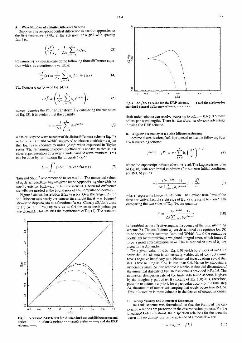
Figure 3 shows the relation a AJC vs a AJC. Over the range a A* upto 1.0 the curve is nearly the same as the straight line a = a. Figure 4shows the slope da /da as a function of a Ax. Clearly da/da is closeto 1.0 (within 0.3%) up to ot AJC — 0.9 (or seven mesh points perwavelength). This satisfies the requirement of Eq. (1). The standard

0.0 0.2 0.6 0.8aAx

Fig. 4 da/da vs a AJC for the DRP scheme, ——; and the sixth-orderstandard central difference s c h e m e , . . . . . . . . . .

sixth-order scheme can resolve waves up to a Ax = 0.6 (10.5 meshpoints per wavelength). There is, therefore, an obvious advantagein using the DRP scheme.

B. Angular Frequency of a Finite Difference SchemeFor time discretization, Ref. 6 proposed to use the following four

levels marching scheme:(n-j)

(8)

where the superscript indicates the time level. The Laplace transformof Eq. (8) with zero initial condition (for nonzero initial condition,see Ref. 6) yields

-1)dt (9)

where ~ represents Laplace transform. The Laplace transform of thetime derivative, i.e., the right side of Eq. (9), is equal to —icof. Oncomparing the two sides of Eq. (9), the quantity

-1) (10)

1.2 1.6 2.0aAx

Fig. 3 OL AJC vs a AJC relation for the standard central difference secondo r d e r , . . . . . . . . . ; fourth order, - - - - - ; sixth order, — • —; and the DRPscheme, ——.

is identified as the effective angular frequency of the time marchingscheme (8). The coefficients bj are determined by requiring Eq. (8)to be second order accurate. Tarn and Webb6 found the remainingcoefficient by minimizing a weighted integral error, which forces a)to be a good approximation of CD. The numerical values of bj aregiven in the Appendix.

For a given value of cbAt, Eq. (10) yields four roots of CD At. Inorder that the scheme is numerically stable, all of the roots musthave a negative imaginary part. Numerical investigations reveal thatthis is true as long as cbAt is less than 0.4. Hence by choosing asufficiently small At, the scheme is stable. A detailed discussion ofthe numerical stability of the DRP scheme is provided in Ref. 6. Thenumerical dissipation rate of the finite difference scheme is givenby the imaginary part of a>. By means of Eq. (10) it is, therefore,possible to estimate a priori, for a particular choice of the time stepAt, the amount of numerical damping that would occur (see Ref. 6).This information is most valuable in the design of computer codes.

C. Group Velocity and Numerical DispersionThe DRP scheme was formulated so that the forms of the dis-

persion relations are preserved in the discretization process. For thelinearized Euler equations, the dispersion relations for the acousticwaves in two dimensions in the absence of a mean flow are

a) = ±a()(ot2 + (11)

1792 TAM

The corresponding dispersion relations for the DRP scheme are[obtained by replacing co, a, and ft by &>, a, and ft in Eq. (11)]

The group velocity11 of the acoustic waves of the DRP scheme canbe obtained by differentiating Eq. (12) with respect to a and ft. It isstraightforward to find

da '±a() da -

da '

If a small At is used in the computation, then cb ~ a; so that(do)/d&>) ~ 1.0. For plane acoustic waves propagating in the xdirection (ft = Q), the wave velocity given by Eq. (13) reduces to

3 CD da— = ±00-7-3 a da

(14)

It is clear from Eq. (14) and Fig. 4 that different wave numbers willpropagate at different speeds. The dispersiveness of a numericalscheme is, therefore, dependent largely on the slope of the numer-ical wave number curve. For the seven-point DRP scheme, da/dadeviates increasingly from 1.0 for a Ax > 1.0 (see Fig. 4). The wavespeed of the short waves (high wave number) is not equal to #0-In fact, for the ultrashort waves (a Ax ~ TT) with wavelengths ofabout two mesh spacings (grid-to-grid oscillations) the group veloc-ity is negative and highly supersonic. The short waves are spuriousnumerical waves. Once excited they would contaminate and degradethe numerical solution.

To illustrate the effect of numerical dispersion, let us consider thesolution of the wave equation

(15)

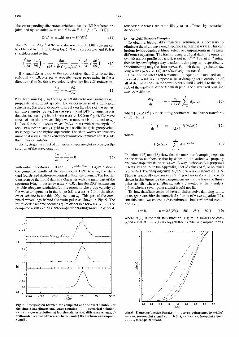
with initial condition t = 0 and u = e~ f«"2(*/3A*) . Figure 5 showsthe computed results of the seven-point DRP scheme, the stan-dard fourth- and sixth-order central difference schemes. The Fouriertransform of the initial data is a Gaussian with the main part of thespectrum lying in the range a Ax < 1.0. Thus the DRP scheme canprovide adequate resolution for this problem. The group velocity ofthe wave components in the range 0.8 < a Ax < 1.0 of the sixth-order scheme is considerably less than #o. This part of the com-puted waves lags behind the main pulse as shown in Fig. 5. Thefourth-order scheme becomes quite dispersive for a Ax > 0.6. Thecomputed result exhibits large-amplitude trailing waves. In general,

0.6

0.4

U 0.2

0.0

a)

b)

c)

0.4

U 0.2

0.0

-0.2390.0

X/&X

Fig. 5 Comparison between the computed and the exact solutions ofthe simple one-dimensional wave equation; ——, numerical solution;. . . . . . . . . 9 exact solution: a) fourth-order central difference scheme, b)sixth-order central difference scheme, and c) DRP scheme (seven-pointstencil).

low-order schemes are more likely to be affected by numericaldispersion.

D. Artificial Selective DampingTo obtain a high-quality numerical solution, it is necessary to

eliminate the short wavelength spurious numerical waves. This canbe done by introducing artificial selective damping terms in the finitedifference equations. The idea of using artificial damping terms tosmooth out the profile of a shock is not new.13'14 Tarn et al.15 refinethe idea by developing a way to tailor the damping terms specificallyfor eliminating only the short waves. For their damping scheme, thelong waves (a Ax < 1.0) are effectively untouched.

Consider the linearized w-momentum equation discretized on amesh of spacing AJC. Suppose a linear damping term consisting ofall of the values of u in the seven-point stencil is added to the rightside of the equation. At the ith mesh point, the discretized equationmay be written as

dt(16)

j =-3

where [va/( Ax)2] is the damping coefficient. The Fourier transformofEq. (16) is

dii •D(aAx)u

where

D(aAx) = e-ijuAx

(17)

(18)

Equations (17) and (18) show that the amount of damping dependson the wave numbers so that by choosing the various dj properlyone can damp only the short waves. A way to choose dj is proposedin Refs. 12 and 15. In the Appendix, a set of values of dj so obtainedis provided. The damping curve D(a Ax) vs a Ax is shown in Fig. 6.There is practically no damping for long waves (a Ax < 1.0). Alsoshown in this figure are the damping curves for the five- and three-point stencils. These smaller stencils are needed at the boundarypoints where a seven-point stencil would not fit.

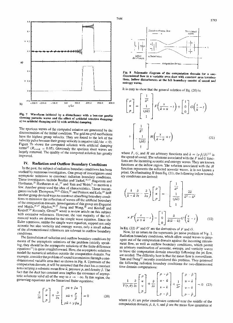
To show the effectiveness of the artificial selective damping terms,let us again consider the numerical solution of wave equation (15).But this time, we choose a discontinuous "box-car" initial condi-tion, i.e.,

= 0, u = Q.5[H(x + 50) - H(x - 50)] (19)

where H(x) is the unit step function. Figure 7a shows the com-puted result at t = 200(Ajc/ao) without artificial damping terms.

0.0 0.4 0.8 1.2 1.6 2.0 2.4 2.8 3.2aAx

Fig.6 Damping function D(ctAx): ——, seven-point stencil (cr = 0.2?r);— • —, seven-point stencil (a = 0.37r); . . . . . . . . . . five-point stencil;- - - - - , three-point stencil.

TAM

0.4

U 0.2

0.4

U 0.2

I M M U . . I M . . . . M . I M M M M . I M . . . . . . . I M . .

\

U^^.1

/ —— \

-

-

-

-

,

-300.0 -200.0 -100.0 0.0 100.0 200.0 300.0 400.0x/Ax

1793

b)

Fig. 7 Waveform initiated by a disturbance with a box-car profileshowing parasite waves and the effect of artificial selective damping:a) no artificial damping and b) with artificial damping.

The spurious waves of the computed solution are generated by thediscontinuities of the initial condition. The grid-to-grid oscillationshave the highest group velocity. They are found to the left of thevelocity pulse because their group velocity is negative (da/da < 0).Figure 7b shows the computed solution with artificial dampingterms (/?stencil = 0.05). Obviously the spurious short waves arelargely removed. The quality of the computed solution has greatlyimproved.

IV. Radiation and Outflow Boundary ConditionsIn the past, the subject of radiation boundary conditions has been

studied by numerous investigators. One group of investigators usedasymptotic solutions to construct radiation boundary conditionsThese investigators include Bayliss and Turkel,16'17 Hagstrom andHanharan,18 Hariharan et al.,19 and Tarn and Webb,6 to mention afew. Another group used the idea of characteristics. These investi-gators include Thompson,20-21 Giles,22 and Poinsot and Lele.23 Stillanother group devised ways to construct absorbing boundary condi-tions to minimize the reflection of waves off the artificial boundaryof the computation domain. Investigators of this group areEngquistand Majda,24-25 Higdon,26-27 Jiang and Wong,28 and Kosloff andKosloff. Recently, Givoli30 wrote a review article on this subjectwith extensive references. However, the vast majority of the ref-erenced works are devoted to the simple wave equation. Since theEuler equations, unlike the simple wave equation, support not onlyacoustic but also vorticity and entropy waves, only a small subsetof the aforementioned references are relevant to outflow boundarvconditions.

The formulation of radiation and outflow boundary conditions bymeans of the asymptotic solutions of the problem (strictly speak-ing, they should be the asymptotic solutions of the finite differenceequations3 ) is quite straightforward. Here, the asymptotic solutionsmodel the numerical solution outside the computation domain. Forexample, consider the problem of sound transmission through a one-dimensional variable area duct as shown in Fig. 8. Upstream of thecomputation domain, it will be assumed that the duct has a constantarea carrying a subsonic mean flow u, pressure p, and density p Thefact that the duct has constant area implies the existence of asymp-totic solutions valid all of the way to x -> -oo. In this region thegoverning equations are the linearized Euler equations:

pu -f pu

uu+ 4p__pu + ypu _

= 0 (20)

Fig. 8 Schematic diagram of the computation domain for a one-dimensional flow in a variable area duct with constant area termina-tions. Inflow disturbances at the left boundary consist of sound andentropy waves.

It is easy to show that the general solution of Eq. (20) is

J_

-L F(^~')+ °(pa) \a u J Q

1

1

(21)

where F, G, and # are arbitrary functions and a = ( y p / p ) l / 2 isthe speed of sound. The solutions associated with the F and G func-tions are the incoming acoustic and entropy waves. They are knownfunctions at the inflow region. The solution associated with the Hfunction represents the reflected acoustic waves. It is not known apriori. On eliminating H fromEq. (21), the following inflow bound-ary conditions are derived:

(-!-*-*-}\a-uBt dxj

Pu

-P.

1a2

1(pa)

I

2aT2

r , x~~(jr I —

u(a-u) \u (22)

In Eq. (22) F' and G' are the derivatives of F and G.Now, let us return to the supersonic jet noise problem of Fig. 1.

Radiation boundary conditions, which allow sound waves to prop-agate out of the computation domain against the incoming entrain-ment flow, as well as outflow boundary conditions, which permitan arbitrary combination of acoustic, entropy, and vorticity wavesto leave the computation domain smoothly following the jet flow,are needed. The difficulty here is that the mean flow is nonuniform!Tarn and Dong32 recently considered this problem. They proposedthe following radiation boundary conditions for two-dimensionaltime domain computations:

1V(r,9)3t

P- Pu — u

V — V

-P- p j

p ~" p

u — u

V — V-0 (23)

_p — p

where (r, 6) are polar coordinates centered near the middle of thecomputation domain; p, u, v, and p are the mean flow quantities at

1794 TAM

the boundary region; and V(r, 0) is related to the mean flow velocityV — (u, v) and the sound speed a by

[a2 - (V • e9)2] * (24)

For the outflow, they proposed a set of boundary conditions that ac-counts for mean flow nonuniformity. If the flow is uniform Eq. (23)and the corresponding outflow boundary conditions reduce to thoseof Tarn and Webb,6 which were derived from the asymptotic so-lutions of the linearized Euler equations by the method of Fouriertransform.

Recently, Hixon et al.33 tested computationally the effectivenessof the radiation and outflow boundary conditions of Thompson,20'21

Giles,22 and Tarn and Webb.6 Their finding was that the bound-ary conditions based on asymptotic solutions performed well, butthe characteristic boundary conditions produced significant reflec-tions. Others also reported similar experience. It is worthwhile topoint out that for two- or three-dimensional problems, there are nogenuine characteristics. Whenever the waves incident obliquely onthe boundary or there is a significant component of mean velocityparallel to the boundary, the validity of any pseudocharacteristicformulation of boundary conditions becomes suspected. Great careshould be exercised in their usage.

V. Computation of Nonlinear Acoustic WavesNonlinearity causes the waveform of an acoustic pulse to steepen

up and ultimately to form a shock. In the study of Tarn and Shen,12 itwas found that the nonlinear wave steepening process, when viewedin the wave number space, corresponded to an energy cascadeprocess whereby low wave number components are transferred tothe high wave number range. If a high-order finite difference schemewith a large bandwidth of long waves (waves with a ~ a) in thewave number space is used for the computation, the computed non-linear waveform remains accurate as long as the cascading processdoes not transfer wave components into the unresolved (short) wavenumber range. Since, in most aeroacoustic problems, the sound in-tensity is not sufficient to cause the formation of acoustic shocks,the use of a high-order finite difference scheme such as the DRPscheme would generally be quite adequate.

If shocks are formed, it is known that high-order schemes gener-ally produce spurious spatial oscillations around them and in regionswith steep gradients. These spurious spatial oscillations are waves inthe short wave (high wave number) range generated by the nonlinearwave cascading process. The high-order ENO10 scheme was con-ceived and designed to have shock-capturing capability. It should be

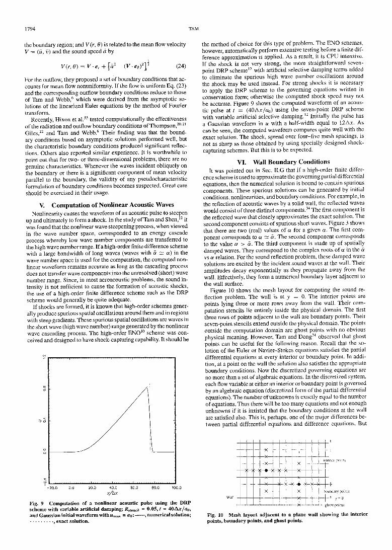
Fig. 9 Computation of a nonlinear acoustic pulse using the DRPscheme with variable artificial damping; Rstendi = 0.05, t = 40Ajc/a0,and Gaussian initial waveform with Mmax = 0o: ——> numerical solution;. . . . . . . . . 9 exact solution.

the method of choice for this type of problem. The ENO schemes,however, automatically perform extensive testing before a finite dif-ference approximation is applied. As a result, it is CPU intensive.If the shock is not very strong, the more straightforward seven-point DRP scheme12 with artificial selective damping terms addedto eliminate the spurious high wave number oscillations aroundthe shock may be used instead. For strong shocks it is necessaryto apply the DRP scheme to the governing equations written inconservation form; otherwise the computed shock speed may notbe accurate. Figure 9 shows the computed waveform of an acous-tic pulse at t — (40Ajt/0()) using the seven-point DRP schemewith variable artificial selective damping.12 Initially the pulse hasa Gaussian waveform in u with a half-width equal to 12Ax. Ascan be seen, the computed waveform compares quite well with theexact solution. The shock, spread over four-five mesh spacings, isnot as sharp as those obtained by using specially designed shock-capturing schemes. But this is to be expected.

VI. Wall Boundary ConditionsIt was pointed out in Sec. II.G that if a high-order finite differ-

ence scheme is used to approximate the governing partial differentialequations, then the numerical solution is bound to contain spuriouscomponents. These spurious solutions can be generated by initialconditions, nonlinearities, and boundary conditions. For example, inthe reflection of acoustic waves by a solid wall, the reflected waveswould consist of three distinct components.34 The first component isthe reflected wave that closely approximates the exact solution. Thesecond component consists of spurious short waves. Figure 3 showsthat there are two (real) values of a for a given a. The first com-ponent corresponds to a ~ a. The second component correspondsto the value a > ct. The third component is made up of spatiallydamped waves. They correspond to the complex roots of a in the avs a relation. For the sound reflection problem, these damped wavesolutions are excited by the incident sound waves at the wall. Theiramplitudes decay exponentially as they propagate away from thewall. Effectively, they form a numerical boundary layer adjacent tothe wall surface.

Figure 10 shows the mesh layout for computing the sound re-flection problem. The wall is at y = 0. The interior points arepoints lying three or more rows away from the wall. Their com-putation stencils lie entirely inside the physical domain. The firstthree rows of points adjacent to the wall are boundary points. Theirseven-point stencils extend outside the physical domain. The pointsoutside the computation domain are ghost points with no obviousphysical meaning. However, Tarn and Dong34 observed that ghostpoints can be useful for the following reason. Recall that the so-lution of the Euler or Navier-Stokes equations satisfies the partialdifferential equations at every interior or boundary point. In addi-tion, at a point on the wall the solution also satisfies the appropriateboundary conditions. Now the discretized governing equations areno more than a set of algebraic equations. In the discretized system,each flow variable at either an interior or boundary point is governedby an algebraic equation (discretized form of the partial differentialequations). The number of unknowns is exactly equal to the numberof equations. Thus there will be too many equations and not enoughunknowns if it is insisted that the boundary conditions at the wallare satisfied also. This is, perhaps, one of the major differences be-tween partial differential equations and difference equations. But

Wall

uenor points

boundary points

•*• y = 0— ghost points

Fig. 10 Mesh layout adjacent to a plane wall showing the interiorpoints, boundary points, and ghost points.

TAM 1795

now the extra conditions imposed on the flow variables by the wallboundary conditions can be satisfied if ghost values are introduced(extra unknowns). The number of ghost values is arbitrary, but theminimum number must be equal to the number of boundary condi-tions. Tarn and Dong suggested to use one ghost value per bound-ary point per physical boundary condition. To eliminate the needfor extra ghost values, they employed backward difference sten-cils to approximate the spatial derivatives at the boundary points.For the plane wall problem, their analysis indicated that the pre-ceding wall boundary treatment would only give rise to very lowamplitude spurious reflected waves. The thickness of the numericalboundary layer was also very small regardless of the angle of inci-dence even when only six mesh points per wavelength were used inthe computation.

In most aeroacoustics problems, the wall surface is curved. InCFD, the standard approach is to map the physical domain into arectangular computational domain with the curved surface mappedinto a plane boundary or use unstructured grids. For aeroacous-tic problems, this is not necessarily the best method. Mapping orunstructured grids effectively introduce inhomogeneities into thegoverning equations. Such inhomogeneities could cause unintendedacoustic refraction and scattering. An alternative way is to retain aCartesian mesh and to develop special treatments for curved walls.Kurbatskii and Tarn35 developed one such treatment by extendingthe one ghost value per boundary point per physical boundary con-dition of Tarn and Dong.34 They tested their curved wall bound-ary conditions by solving a series of linear two-dimensional acous-tic wave scattering problems. Morris et al.36 proposed not to usethe wall boundary condition. Instead they simulated the change inimpedance at the wall by increasing the density of the fluid insidethe solid body. At this time, it is too early to judge how well thesealternative methods would perform in problems with complex wallboundaries. But for problems involving simple scatterers such as cir-cular and elliptic cylinders, excellent computed results of the entiredscattered acoustic field have been obtained.35 In any case, mappingor unstructured grids may not be absolutely necessary for aero-acoustics problems.

VII. Concluding RemarksAs a subdiscipline, CAA is still in its infancy. In this paper, some

of the relevant computational issues and methods are discussed (fora set of benchmark problems designed to address some of these is-sues see Ref. 37). Obviously, the development of new methods isvery much needed. However, it is also pertinent to echo the beliefthat applications of CAA to important or as yet unsolved aeroacous-tics problems are just as needed. It is necessary to demonstrate theusefulness, reliability, and robustness of CAA. Unless and until thisis accomplished, CAA will remain merely a research subject but notan engineering tool.

Appendix: Stencil and Damping CoefficientsThe coefficients of the seven-point DRP scheme are

ao = 0 ai = -a_! = 0.770882380518a2 = -a-2 = -0.166705904415a3 = -a_3 = 0.208431427703

Backward stencil coefficients are a"m, j = — n, — n +1, . . . , m — 1,m (n — number of points to the left and m = number of points tothe right):

a™ = -a™ = -2.192280339ao6 = _a60 = 4.748611401

006 = _fl(G» = _5.io8851915

of = -a™3 = 4.461567104af = -a™4 = -2.833498741af = -fl«= 1.128328861

fl06 _ _fl6o _ -0.203876371

al_\ = -al1 = -0.209337622al

Q5 = -al1 = -1.084875676

a}5 = -a5_\ = 2.147776050al

25 = -a5_\ = -1.388928322

a*5 = -a5_\ = 0.768949766al

45 = -a5_\ = -0.281814650

al55 = -a^5 = 0.048230454

*-2 = ~fl22 = 0.049041958a2^ = -af = -0.468840357a™ = -af = -0.474760914a24 = -a42! = 1.273274737

a24 = -a422 = -0.518484526

a24 = -a423 = 0.166138533

a24 = -a424 = -0.026369431

The coefficients of the four-level time-marching stencil are

bo = 2.302558088838bi = -2.491007599848b2 = 1.574340933182

b3 = -0.385891422172

The coefficients of the seven-point damping stencil are

(or = 0.27T) (a = Q.37T)

do = 0.287392842460 0.327698660845di = <Li = -0.226146951809 -0.235718815308d2 = d.2 = 0.106303578770 0.086150669577

d3 = d_3 = -0.023853048191 -0.014281184692

The coefficients of the five-point damping stencil are

d0 = 0.375di = J_i = -0.25d2 = d-2 = 0.0625

The coefficients of the three-point stencil are

d0 = 0.5, di = d-i = -0.25

AcknowledgmentsThis work was supported by NASA Lewis Research Center Grant

NAG 3-1267. Part of this work was written while the author wasin residence at the Institute for Computer Applications in Scienceand Engineering. The author wishes to thank Hao Shen and DavidKopriva for their assistance.

References*Hubbard, H. H. (ed.), Aeroacoustics of Flight Vehicles: Theory and

Practice, Vol. 1: Noise Sources, Vol. 2: Noise Control, NASA RP-1258,Aug. 1991.

2Tam, C. K. W., "Jet Noise Generated by Large-Scale Coherent Mo-tion," Aeroacoustics of Flight Vehicles, NASA RP-1258, Aug. 1991, Chap.6, pp. 311-390.

3Tam, C. K. W., "Supersonic Jet Noise," Annual Review of Fluid Mechan-ics, Vol. 27,1995, pp. 17-43.

4Seiner, J. M., "Advances in High-Speed Jet Aeroacoustics," AIAA Paper84-2275, Oct. 1984.

5Roe, P. L., "Technical Prospects for Computational Aeroacoustics,"AIAA Paper 92-02-032, May 1992.

6Tam, C. K. W., and Webb, J. C., "Dispersion-Relation-Preserving FiniteDifference Schemes for Computational Acoustics," Journal of Computa-tional Physics, Vol. 107, Aug. 1993, pp. 262-281.

7Thomas, J. P., and Roe, P. L., "Development of Non-Dissipative Numer-ical Schemes for Computational Aeroacoustics," AIAA Paper 93-3382, July1993.

8Zingg, D. W., Lomax, H., and Jurgens, H., "An Optimized Finite Differ-ence Scheme for Wave Propagation Problems," AIAA Paper 93-0459, Jan.1993.

9Lockard, D. P., Brentner, K. S., and Atkins, H. L., "High AccuracyAlgorithms for Computational Aeroacoustics," AIAA Paper 94-0460, Jan.1994.

10Harten, A., Engquist, A., Osher, S., and Chakravarthy, S., "UniformlyHigh-Order Accuracy Essentially Non-Oscillatory Schemes III," Journal ofComputational Physics, Vol. 71, Aug. 1987, pp. 231-323.

11 Whitham, G. B., Linear and Nonlinear Waves, Wiley-Interscience, NewYork, 1974.

1796 TAM

12Tam, C. K. W., and Shen, H., "Direct Computation of Nonlinear Acous-tic Pulses Using High-Order Finite Difference Schemes," AIAA Paper 93-4325, Oct. 1993.

13 Von Neumann, J., and Richtmyer, R. D., "A Method for the NumericalCalculation of Hydrodynamic Shocks," Journal of Applied Physics, Vol. 21,March 1950, pp. 232-237.

14Jameson, A., Schmidt, W., and Turkel, E., "Numerical Solutions ofthe Euler Equations by Finite Volume Methods Using Runge-Kutta TimeStepping Schemes," AIAA Paper 81-1259, June 1981.

15Tam, C. K. W., Webb, J. C., and Dong, Z., "A Study of the Short WaveComponents in Computational Acoustics" Journal of Computational Acous-tics, Vol. 1, March 1993, pp. 1-30.

16Bayliss, A., and Turkel, E., "Radiation Boundary Conditions for Wave-Like Equations," Communications on Pure and Applied Mathematics, Vol.33, Nov. 1980, pp. 707-725.

17Bayliss, A., and Turkel, E., "Far Field Boundary Conditions for Com-pressible Flows," Journal of Computational Physics, Vol. 48, Nov. 1982, pp.182-199.

18Hagstrom, T., and Hariharan, S. L, "Accurate Boundary Conditions forExterior Problems in Gas Dynamics," Mathematics of Computation, Vol. 51,Oct. 1988, pp. 581-597.

19Hariharan, S. I., Ping, Y., and Scott, J. C., "Time Domain NumericalCalculations of Unsteady Vortical Flows About a Flat Plate Airfoil," Journalof Computational Physics, Vol. 101, Aug. 1992, pp. 419-430.

20Thompson, K. W, "Time Dependent Boundary Conditions for Hyper-bolic Systems," Journal of Computational Physics, Vol. 68, Jan. 1987, pp.1-24.

21 Thompson, K. W., "Time Dependent Boundary Conditions for Hyper-bolic Systems, II," Journal of Computational Physics, Vol. 89, Aug. 1990,pp. 439^61.

22Giles, M. B., "Nonreflecting Boundary Conditions for Euler EquationCalculations," AIAA Journal, Vol. 28, No. 12, 1990, pp. 2050-2058.

23Poinsot, T. J., and Lele, S. K., "Boundary Conditions for Direct Simu-lations of Compressible Viscous Flows," Journal of Computational Physics,Vol. 101, July 1992, pp. 104-129.

24Engquist, B., and Majda, A., "Radiation Boundary Conditions forAcoustic and Elastic Wave Calculations," Communications on Pure andApplied Mathematics, Vol. 32, May 1979, pp. 313-357.

25Engquist, B., and Majda, A., "Absorbing Boundary Conditions for the

Numerical Simulation of Waves," Mathematics of Computation, Vol. 31,July 1977, pp. 629-651.

26Higdon, R. L., "Absorbing Boundary Conditions for Difference Ap-proximations to the Multi-Dimensional Wave Equation," Mathematics ofComputation, Vol. 47, Oct. 1986, pp. 629-651.

27Higdon, R. L., "Numerical Absorbing Boundary Conditions forthe Wave Equation," Mathematics of Computation, Vol. 49, July 1987,pp. 65-90.

28 Jiang, H., and Wong, Y. S., "Absorbing Boundary Conditions for SecondOrder Hyperbolic Equations," Journal of Computational Physics, Vol. 88,May 1990, pp. 205-231.

29Kosloff, R., and Kosloff, D., "Absorbing Boundaries for Wave Propa-gation Problems," Journal of Computational Physics, Vol. 63, April 1986,pp. 363-376.

3()Givoli, D., "Non-Reflecting Boundary Conditions," Journal of Compu-tational Physics, Vol. 94, May 1991, pp. 1-29.

31 Tarn, C. K. W., and Webb, J. C., "Radiation Boundary Condition andAnisotropy Correction for Finite Difference Solutions of the HelmholtzEquation," Journal of Computational Physics, Vol. 113, July 1994, pp.122-133.

32Tam, C. K. W, and Dong, Z., "Radiation and Outflow Boundary Con-ditions for Direct Computation of Acoustic and Flow Disturbances in aNonuniform Mean Flow," AIAA Paper 95-007, June 1995.

33Hixon, D. R., Shih, S., and Mankbadi, R. R., "Evaluation of BoundaryConditions for Computational Aeroacoustics," AIAA Paper 95-0160, Jan.1995.

34Tam, C. K. W, and Dong, Z., "Wall Boundary Conditions for High-Order Finite Difference Schemes in Computational Aeroacoustics," Theo-retical and Computational Fluid Dynamics, Vol. 8, No. 6,1994, pp. 303-322.

35Kurbatskii, K. A., and Tarn, C. K. W, "Curved Wall Boundary Condi-tions for High-Order Finite Difference Schemes in Acoustic Wave ScatteringProblems," Bulletin of the American Physical Society, Vol. 39, Nov. 1994,p.1907.

36Morris, P. J., Chung, C., Chyczewski, T. S., and Long, L. N., "Computa-tional Aeroacoustics Algorithms: Nonuniform Grids," AIAA Paper 94-2295,June 1994.

37Hardin, J. C. (ed.), Computational Aeroacoustics Benchmark Problems,Proceeding of the ICASE/LaRC Workshop on Benchmark Problems in Com-putational Aeroacoustics (Hampton, VA), NASA CP-3300, May 1995.