Embed Size (px)
Citation preview
Effective Protection, Domestic Resource Costs,and Shadow Prices
A General Equilibrium Perspect;-^--
Edward Tower SWP664
WORLD BANK STAFF WORKING PAPERSNumber 664
Pub
lic D
iscl
osur
e A
utho
rized
Pub
lic D
iscl
osur
e A
utho
rized
Pub
lic D
iscl
osur
e A
utho
rized
Pub
lic D
iscl
osur
e A
utho
rized
Pub
lic D
iscl
osur
e A
utho
rized
Pub
lic D
iscl
osur
e A
utho
rized
Pub
lic D
iscl
osur
e A
utho
rized
Pub
lic D
iscl
osur
e A
utho
rized

WORLD BANK STAFF WORKING PAPERSNumber 664
Effective Protection, Domestic Resource Costs,and Shadow Prices
A General Equilibrium Perspective
Edward Tower
jIR1ERNATIONAL yO?tTARIlY FUNDJOINT LIBRABY
RECO.iU7'13CN aNsM M1D_'ELOPlHENTVIAESIMC-NTC14 D,C. -43
The World BankWashington, D.C., U.S.A.
Copyright (© 1984The Intemational Bank for Reconstructionand Development/THE WORLD BANK1818 H Street, N.W.Washington, D.C. 20433, U.S.A.
All rights reservedManufactured in the United States of AmericaFirst printing September 1984
This is a working document published informally by the World Bank. To present theresults of research with the least possible delay, the typescript has not been preparedin accordance with the procedures appropriate to formal printed texts, and theWorld Bank accepts no responsibility for errors. The publication is supplied at atoken charge to defray part of the cost of manufacture and distribution.
The views and interpretations in this document are those of the author(s) andshould not be attributed to the World Bank, to its affiliated organizations, or to anyindividual acting on their behalf. Any maps used have been prepared solely for theconvenience of the readers; the denominations used and the boundaries shown donot imply, on the part of the World Bank and its affiliates, any judgment on thelegal status of any territory or any endorsement or acceptance of such boundaries.
The full range of World Bank publications, both free and for sale, is described inthe Catalog of Publications; the continuing research program is outlined in Abstracts ofCurrent Studies. Both booklets are updated annually; the most recent edition of eachis available without charge from the Publications Sales Unit, Department T, TheWorld Bank, 1818 H Street, N.W., Washington, D.C. 20433, U.S.A., or from theEuropean Office of the Bank, 66 avenue d'1ena, 75116 Paris, France.
Edward Tower, a consultant to the Industry Department of the World Bank, isprofessor of economics at Duke University.
Library of Congress Cataloging in Publication Data
Tower, Edward.Effective protection, domestic resource costs, and
shadow prices.
(World Bank staff working papers ; no. 664)Bibliography: p.1. Tariff--Mathematical models. 2. Commercial policy--
Mathematical models. 3. Economic policy--Mathematicalmodels. 4. Shadow prices. 5. Equilibrium (Economics)6. Second best, Theory of. I. Title. II. Series.HF1713.T69 1984 382.7'0724 84-17307ISBN 0-8213-0404-6
ABSTRACT
Simple general equilibrium models are built, linearized about
their initial equilibrium, and then used to analyze the economic effects
of various changes in policy. In the process, the models are used to
elucidate effective protection, shadow prices, and domestic resource cost
and the relationships among them. In particular, the paper discusses
applications to simple approaches to second-best tariffs, including
second-best optimum tariffs on imported capital goods; alternative defi-
nitions of nominal and effective rates of protection; the symmetry between
effective protection and value added subsidies; the relation between
effective protection and shadow prices, and the relationship between the
effective rate of protection and domestic resource cost.
EXTRACTO
Se construyen modelos de equilibrio general simples, linearizados en
torno a su equilibrio inicial, y luego se usan para analizar los efectos eco-
n6micos de diversas modificaciones de politica. En el anAlisis los modelos se
usan para explicar la protecci6n efectiva, los precios sombra y el costo de
los recursos internos, asi como las relaciones entre ellos. En particular, en
este trabajo se examinan: la aplicaci6n de m6todos sencillos para estimar los
aranceles que siguen a los mejores, incluidos los aranceles que siguen a los
6ptimos sobre los bienes de capital importados; distintas tasas de protecci6n
nominales y efectivas; la simetria entre la protecci6n efectiva y las subven-
ciones al valor agregado; la relaci6n entre protecci6n efectiva y precios
sombra, y la relaci6n entre las tasas efectivas de protecci6n y el costo de
los recursos internos.
Pour analyser les consequences economiques qu'entrainent
certains changements de politique, l'auteur construit des modeles simples
d'equilibre gen6ral et les linearise autour de leur position d'equilibre
initiale. Ces modeles servent a evaluer la protection effective, les prix
de ref6rence et les coats en ressources interieures, ainsi qu'a mettre en
lumiere les relations qui existent entre ces el6ments. Le document porte
en particulier sur les points suivants : application des modeles a des
methodes simples d'estimation des droits de douane a appliquer, et notam-
ment du niveau optimal des droits applicables aux biens d'investissement
importes, a defaut de pouvoir modifier d'autres droits; analyse critique
des definitions du taux nominal et du taux effectif de protection; syme-
trie existant entre la protection effective et les subventions a la valeur
ajoutee; relation entre la protection effective et les prix de r6f6rence,
et relations existant entre les taux effectifs de protection et des coats
en ressources interieures.
ACKNOWLEDGMENTS
This paper was written while the author (who teaches at Duke
University) was consulting at the World Bank's Industrial Development and
Finance Department (which subsequently became the present Industrial
Strategy and Policy Division of the Industry Department) in connection with
the Incentives and Comparative Advantage (INCA) Unit research project (RPO
672-44). The INCA Unit was established to support the many studies at the
Bank and in developing countries, which involve the estimation of empirical
incentive and cost-benefit (comparative advantage) indicators. The paper,
which provides an up-to-date review of a very extensive theoretical
literature, forms part of the INCA Unit's creation of an infrastructure for
facilitating this work. It was written under the supervision of Garry
Pursell who directs the INCA Unit project. Both he and Neil Roger were
instrumental in its formulation and development by suggesting new ideas and
helping refine old ones. The author is also grateful to the following
people (both Bank staff members and others) for helpful guidance and
criticism along the way: Bela Balassa, Trent Bertrand, Max Corden, Kemal
Dervis, Peter Dixon, Sebastian Edwards, David Feldman, Alice Galenson,
Khuan-Poh Gan, Jim Hartigan, Kiyoun Han, Tom Hutcheson, Gordon Hughes, Kent
Kimbrough, Andrea Maneschi (who made line by line comments on the entire
manuscript), David Newbery, Pradeep Mitra, Demetrios Papageorgiou,
Anandarup Ray, Barbara L. Rollinson, Lyn Squire, Nobu Teramachi and Mateen
Thobani. Thanks also go to Wanda Jedierowski and Pat Johnson for typing
various versions as the paper has grown and the notation has changed.
TABLE OF CONTENTS
Chapter I - INTRODUCTION AND SUMMARY .................................. . 1
Chapter II - A FRAMEWORK FOR CALCULATING SHADOW PRICES OF GOODS, FACTORS ANDPARAMETERS OF ECONOMIC POLICY ............ ...... ............... . 22
II.1 Introduction.. ............ .... 22
II.2 The Model ..........................................23
II.3 Summary ............-...... -.............. 32
II.4 Solution and Interpretation of Results.............34
II.5 Extensions .... o.oo -o... o..*..* .... o...o.oo...............43
Chapter III -APPLICATIONS TO SECOND BEST TARIFFS................ . .......51
III.1 On a Quick and Simple Approach to Estimating Second BestTariffs .,oo................. o*.o...... ooo.o... 9- ... 51
III.2 On Using a Single Tariff to Exploit Market Power on ManyTraded Goods.....................o.. ................ 60
III.3 Some Thoughts on the Optimum Tax on Imported CapitalGoods in the Presence of Other Taxes and Tariffs...67
III.4 Optimum Taxes on Imported Capital Goods and Intermediate
III.5 Conclusions, Implications and Extensions...........93
Chapter IV - ON THE SYMMETRY BETWEEN EFFECTIVE TARIFFS AND VALUE ADDEDSUBSIDIES . .......................................... 96
IV.1 Introduction ...... .... 96
IV.2 On Alternative Definitions of the Nominal Rate ofProtection ..... . .............. . 96
IV.3 Theorem and Implications . . 97
IV.4 Defining the ERP and exploring its relationship to theNRP ............................ 101
IV.5 The Equivalence Proposition ....................... 102
IV.6 Additional Equivalence Propositions .... ... 105
IV.7 The Effective Rate of Value Added Subsidy and theImplicit Rate of Final Demand Taxation ............ 107
IV.8 Non-Traded Goods ......... ............... . 108
IV.9 Monopoly Power .................................... 114
IV.10 Absolute Levels of Nominal and Effective ProtectionDon't Matter ...................................... 115
IV.11 The Net Effective Rate of Protection .............. 116
IV.12 Negating the Real Impact of A Tariff Structure....118
IV.13 On Neutrality When There is Substitutability BetweenIntermediate Inputs .............................. . 118
IV.14 On Drawbacks ................ ............... 120
IV.15 Effective Protection as a Value Added Tax and Its Impacton the Exchange Rate .... . ................ 122
IV.16 On A Proposal to Liberalize Trade .................. 122
IV.17 Other Definitions of the ERP . .................. 124
IV.18 Conclusion ........................................ 127
Chapter V - THE IMPLICIT RATE OF FINAL DEMAND TAXATION AND THE EFFECTIVERATE OF VALUE ADDED SUBSIDY AS DETERMINANTS OF SHADOW PRICES................................................. ........................................ 128
V.1 Introduction ...................................... 128
V.2 Deriving the Fundamental Equation ................. 129
V.3 Interpreting the Fundamental Equation ............. 134
V.4 Alternative Reference Prices and Alternative Forms forthe Fundamental Equation ........... 135
V.5 Evaluating Resource Shifts and Calculating Shadow PricesWhen Consumer Prices are Fixed .................... 136
V.6 Calculating Shadow Prices When Consumer Prices areVariable ............ .............................. 139
V.7 Insights for the Shadow Pricer . . . 140
V.8 Generalizing the Interpretation of the FundamentalEquation ................................................ 142
V.9 On Calculating The- Shadow Prices of Distortions and theWelfare Gain From Eliminating Them ............ 144
V.10 The Geometry of A Tariff Cut ...................... 149
V.11 The Welfare Impact of A Resource Shift Under AlternativeWays of Treating Non-Traded Goods ................. 152
V.12 In What Way are Non-Traded Goods a Problem and How Use-ful are Standard Formulae for the Effects of TariffStructures? ...... . ....... 158
Chapter VI - ON THE RELATIONSHIP BETWEEN THE EFFECTIVE RATE OF PROTECTION ANDDOMESTIC RESOURCE COST .................................... 161
VI.1 Introduction .................................................. 161
VI.2 Assumptions and Definitions ........ ................ 162
VI.3 Modeling . .. ......................... 164
VI.4 Major Conclusions ................. ............. . 166
VI.5 The Case of Only One Mobile Factor of Production..167
VI.6 More Than Two Factors of Production, Two Goods and OneTime Period .......... se... .. 168
VI.7 Non-Traded Goods . .............................. . 168
VI.8 The Activity Cost-Benefit Ratio ................... 170
VI.9 How to Use the DRC .. . ....... 171
VI.10 The DRC and The Adjustment Mechanism Assumed ...... 172
VI.11 Is the DRC the Best Cost-Benefit Ratio? ........... 173
REFERENCES ....................................................... 176
CHAPTER I
INTRODUCTION AND SUMMARY
I.1 INTRODUCTION
In many developed and developing countries effective rates of
protection (ERPs) shadow prices and domestic resource cost ratios (DRCs)
are very commonly estimated and used to analyse a variety of trade policy
questions. In this paper we survey some of the theoretical literature on
these subjects with the purpose of elucidating the relationship between
these concepts and how they might be used for making inferences for
economic policy. This is done by building simple general equilibrium
models, linearising them about the initial equilibrium and then solving
them to discover the economic effects of various changes in policy. By so
doing one can gain insights into optimum policies with regard to taxes,
subsidies and direct controls on production, consumption and trade. The
paper is divided into this introduction and five subsequent chapters which
we now summarize.
2
I.2 CHAPTER II
Chapter II, entitled "A Framework for Calculating Shadow Prices
of Goods, Factors and Parameters of Economic Policy," builds a prototype
model for calculating the effects on economic welfare of small changes in
government sales of factors, goods and foreign exchange so that the private
sector gains their services, and of increases in policy parameters like
tariffs, quotas, taxes and subsidies, where economic welfare is assumed to
depend on the real income of two groups and its distribution between them.
It also shows how to calculate the effects of these changed autonomous
variables on other endogenous variables of concern to policy makers.
The model is not designed to be innovative. Rather, it is
intended to describe a simple full-employment specific factor model with
interindustry relationships and variable world prices.
In particular, we assume that each good is produced using inter-
mediate inputs and a value added aggregate in fixed proportions and with
constant returns to scale. Then we let the value-added aggregate be a
constant returns
3
to scale function of one factor which is specific to the industry (i.e. used
only by the industry) and one factor which is mobile between industries. In
the simplest interpretation of our model we interpret the specific factor as a
combination of capital and land which in the short run is difficult to move
from industry to industry and we interpret the mobile factor as labor which is
mobile between industries,I although in the longer run one might wish to think
of most capital and labor being mobile between industries, with only a small
fraction of the capital stock being sector specific. The model has several
purposes.
First and most important, it is designed to present an introduction to
the shadow pricing of goods and policy parameters as a complement to the
Little-Mirrlees (1974) and Squire and Van der Tak (1975) discussions which are
partial equilibrium in exposition. The approach is to recognize that a hypo-
thetical economy can be described as a collection of many relatively simple
relationships or equations, then to linearize the system, and solve it to find
the amount by which welfare changes in response to small increases in policy
parameters and government sales of goods, factors, and foreign exchange. Then
the shadow price of any commodity, factor, or parameter is simply the fall in
welfare which results from a unit increase in the government purchases of that
commodity or factor or an increase in that parameter. To look at the problem
more generally, we can define the policy maker's utility as a function of
various aspects of how the economy performs, e.g. real incomes to various
groups, real government revenues, prices and unemployment rates; and the
shadow price of any parameter, good or factor is simply the ratio of the
increase in the policy maker's utility t6 the increase in the parameter or
'For more on the specific factor model, see Neary (1978).

4
government sales of the good or factor in question. To explain the concept of
shadow prices in this way is important, because practical guides to shadow
pricing sometimes fail to distinguish between the particular technique used to
calculate a shadow price and the meaning of a shadow price.
Secondly, this chapter is intended to be an introduction to the art of
model building, and to encourage people working in the area to think in terms
of general equilibrium.2
Third, this chapter is intended to encourage use of this sort of linear
model for calculating shadow prices. This is because such a model is just as
good as a computable general equilibrium (OGE) model for this purpose, since
what is required is an analysis of only a small perturbation of the system
from its initial equilibrium.3
Fourth, this chapter is designed to encourage readers to recognize that
this kind of model can also be useful as an approximation to the effects of a
set of finite changes in endowments and policy parameters. While it offers
only an approximation to the correct solution for finite changes, it is sim-
pler than a CGE model in three senses: (A) to solve it requires only matrix
2In this regard it performs the same function as chapter 2 of Dixon, Parmeter,Sutton and Vincent (1982), henceforth DPSV (1982), which presents a skeletalversion of their general model in order to give readers a rapid understandingof their approach.
3The strength of a CGE model is that it enables one to calculate to anydesired degree of accuracy the effects of a set of finite changes in para-meters and endowments. But the role of the shadow pricing authority should beto calculate the loss of welfare from small adjustments in government pur-chases and parameters from some base, for that is the definition of a shadowprice. If the base is the observed status quo, both a CGE and a linear modelwill perform equally well. However, if it is believed that the economy isabout to jump or has already jumped from the equilibrium which was used tocalibrate the model to a new one, a finite distance away, one would wish touse a CGE model or else a linear model along with the numerical integrationreferred to in the next footnote to calculate the full description of the newequilibrium. Then to find shadow prices at this new equilibrium a linearmodel, calibrated about the new equilibrium, would be appropriate.
5
multiplication instead of an iterative computer algorithm; (B) such solutions
require knowledge of only first derivatives of the functions, rather than
complete specification of them, and (C) it offers an analytic solution which
recommends its use when a quick answer is required or an analytic solution is
needed in order to better intuit the essence of an analytical problem.4
I.3 CHAPTER III
III. 1
Chapter III uses special cases of the general model developed in the
first chapter to approach particular problems. It consists of several related
essays. The first entitled "On a Quick and Simple Approach to Estimating
Second Best Tariffs" lays out the concept that the welfare gain associated
with the reduction of a particular distortion is equal to the sum of the
induced flows of goods across each of the economy's distortions, each multi-
plied by the size of the distortion attached to that flow. It then shows how,
even when we do not have more than a rough idea of how to model an economy and
for some reason all tariffs but one are frozen, perhaps by political con-
straints, we can get an estimate of what the remaining tariff should be.
This is an example of the use of a very simple model to reach policy con-
clusions using information from policy makers as a major direct input into the
analysis. I believe it is also a good way to introduce the classic problem of
4For the state of the art in OGE modeling see Dervis, DeMelo and Robinson(1982), DPSV (1982) and Harris (1982). For more on the advantages of a linearapproach over a OGE formulation see DPSV (1982, pp. 5, 6 and 47). DPSV (1982,pp. 51-54) also discuss how to use conventional numerical integrationtechniques in conjunction with a linear model with the same mathematicalproperties as the one presented here to obtain exact solutions for finitechanges. Thus the basic framework suggested here is not limited to theconsideration of infinitesimal changes.
6
the general theory of the second best because the solution is at a level that
should be comprehensible to those with a basic mastery of undergraduate
economics.
III.2
The next essay, written jointly with Harold 0. Fried, "On Using a Single
Tariff to Exploit Market Power on Many Traded Goods," considers the same
problem in the context of variable world prices. Thus, in this model, unlike
the previous one, there is an externality from the viewpoint of the home
economy, namely variable terms of trade, which needs internalizing through the
use of tariffs. In this paper, we explain more fully the logic behind the
optimum use of a policy instrument in one market to maximize welfare, when
(using Bhagwati's (1971) terminology) there are both autonomous policy imposed
distortions in other markets (e.g. tariffs we can't do anything about) and
endogenous non-policy imposed distortions (e.g. monopoly power) in all
markets.
The particular policy conclusions which emerge from this essay are that
any policy which increases (reduces) imports of any good with an import tariff
which is above (below) the traditional optimum import tariff (when foreign
excess supply functions are independent of one another this is 1/a,, where a,
is the elasticity of foreign excess supply) is beneficial in that regard.
Similarly, any policy which reduces exports of goods subject to export subsi-
dies or inadequate export taxes is beneficial. Thus one can assess the
desirability of any particular policy by summing up its effects on all imports
and exports. More specifically, the change in domestic real income is given
by the policy-induced increased net imports (in physical terms) multiplied by
the amount by which the wedge between domestic and world prices exceeds what
7
it ought to be based on traditional optimum tariff calculations, summed over
all traded commodities.
We then illustrate this general principle by showing how this problem
relates to the case of a less developed economy which imports both a capital
intensive good and foreign capital services and faces fixed prices for traded
commodities, an upward sloping supply of foreign capital services and a fixed
corporation income tax. Our conclusion is that the introduction of a small
import tariff is welfare increasing if and only if the corporation income tax
exceeds the traditional optimum corporation income tax rate. Then the optimum
import tariff can be determined by recognizing that raising the import tariff
will be beneficial if and only if the capital attracted times the difference
between the marginal product of capital and the marginal expenditure on it
exceeds the quantity of the import repelled times the difference between its
unit value to domestic consumers and its world price.
III.3
The third essay in this chapter, "Some Thoughts on The Optimum Tax on
Imported Capital Goods in The Presence of Other Taxes and Tariffs," goes
beyond the other essays by building a specific model of interactions within
the economy of a hypothetical primary-producing less developed country to
determine the optimum level for one tariff when others are frozen. This essay
is more directly relevant to World Bank problems than the other two as it is
based on an actual problem confronted by a World Bank mission. The analytical
results obtained here are neat, and initially surprising, but are understand-
able intuitively. Thus, this essay both clarifies the forces at work in the
problem and provides some ball-park estimates. It also indicates how one can
simplify a complex problem to manageable proportions.
8
The particular story we tell is of a country which faces fixed world
prices and uses labor and imported capital goods to produce a single good,
some of which is consumed and some of which is exported, with exports subsi-
dized. Moreoever, the earnings from this export are used to import both the
capital good and a consumption good subject to a fixed tariff. One result of
our analysis is that the import tariff on the consumption good is not a deter-
minant of the optimum tariff on imported capital. This is because all
consumption goods are traded with world prices and their border taxes fixed,
so that their domestic prices are fixed. Thus consumption expands or con-
tracts along a given income - consumption line. Therefore (holding savings
constant), domestic utility derived from consumption in any period will be
maximized by maximizing the value at world prices of domestic production net
of capital stock depreciation in each period. Other results are that when
there is no domestic corporation income tax to distort savings behavior, the
optimum tax on imported capital goods will just offset the export subsidy, and
hence will be equal to it. However, when we are forced to reckon with a
positive corporation income tax which discourages savings, it is necessary to
subsidize imported capital goods to offset it. When there is no depreciation
or export subsidy the optimum policy is to subsidize the import of capital
goods at the same rate at which the corporation income tax is levied. Thus
with a corporation income tax of 20% and an export subsidy of 15% we should
levy something between an import subsidy on capital goods of 20% and an import
tariff of 15% on them. Taking the real before tax rate of return on invest-
ment to equal the rate at which capital goods depreciate, we come up with an
optimum import tax on capital goods of 3.5%.
9
III.4
The fourth essay, "Optimum Taxes on Imported Capital Goods and Inter-
mediate Goods" is a further analysis of the problem posed in the previous
essay. The problem was to provide a more detailed analysis which captures
more elements of the problem posed there and allows for the simultaneous
determination of two second best tariffs. In the process it explores some of
the ways of making the analysis tractable, and discovers some of the difficul-
ties associated with making the models more complex. The reader may wish to
skip quickly through much of this essay as it involves some tedious
manipulation.
What this paper tries to describe is a less developed economy which pro-
duces both agricultural goods and manufactured goods where the manufacturing
activity uses labor, imported inputs, agricultural goods and capital to
produce processed agricultural output. We then recognize that some luxury
consumer goods are solely imported, and that the country consumes both the
processed agricultural goods and the non-competitive import. The distortions
are a 20% corporation income tax, a 20% export subsidy on processed agricul-
tural goods and an 80% import tariff on luxury consumer goods. While this is
a very simple economy, it is complex enough to illustrate the principles of
how one would go about analyzing a more complex model. Holding all of our
distortions fixed, but letting the elasticity of supply of domestic savings5
and the elasticity of substitution between land and labor in agriculture vary
between zero and infinity, we find that the optimum import tariff on imported
capital goods varies from -7.7% to 34.2%, while the optimum import tariff on
5We are defining the elasticity of supply of domestic savings as the propor-tional change in the quantity of capital goods that individuals are willing tohold per percentage increase in the after-tax rate of return on capital.
10
non-capital inputs varies from 7.5% to 40.5%. Finally, if we are constrained
to impose a common tariff on all imported inputs it should lie between .74%
and 34.2%. These are of course polar cases; in practice, with realistic
elasticity values, the second best optimal tariffs would fall within a fairly
narrow range between these broad limits.
III.5
Conclusions, implications and extensions of the work contained in chap-
ters two and three are presented in the final essay of Chapter III. These are
the following:
A. The optimum tariffs on intermediate inputs and imported capital goods are
very dependent on the particular parameter values assumed. Thus, attempting
to find second-best tariffs, while simple in theory is likely to be quite
troublesome in practice, both because our knowledge of parameters is uncertain
and because parameters are likely to change from time to time. Therefore, it
is hard to escape the view that the role of the policy adviser should be,
whenever possible, to correct distortions at their source and move the economy
back toward first-best equilibria.
B. This view is reinforced by the fact that comparative static analysis is a
fiction. In truth each market (goods, capital, labor, savings) adjusts at
different speeds, and by convention when we do comparative static analysis we
pick a length of run where some markets have adjusted totally and others not
at all. In fact, in the very short run unemployment should be permitted. In
the long run it is reasonable to assume that most types of unemployment will
disappear, but some capital and some labor is still tied to particular
sectors. In the still longer run a Heckscher - Ohlin model with both capital
and labor internally mobile but with total domestic supplies of labor and
I1
capital fixed may be reasonable. Finally, in the very long run both labor and
capital in the aggregate will be variable. In calculating optimal tariffs
which length of run is reasonable? The answer is none of these. This is
because (1) the policy makers must always trade off short versus long run
costs and benefits and (2) if everyone knows that the economy is going to move
through successive equilibria, it is obvious that the optimum time path of the
vector of tariffs will be complex, and individual decision makers will wish to
reckon with the dynamic path in making their decisions.
C. We can, actually, be somewhat more optimistic than one would expect from a
quick look at the numerical results of section III.4. It is not too surpris-
ing, since we have let two parameters vary between 0 and -, that we got a wide
range of results. In actual fact, the policy adviser is likely to have a
somewhat better idea of what parameter values are likely to be, and should be
able to narrow the range of estimated optimum tariffs accordingly.
D. One important point, which is illustrated by the preceeding section and
elsewhere in the paper, is that one can calculate the welfare impact of a
tariff change as the sum of a set of distortions multiplied each by a cor-
responding change in flows of goods induced by a change in the tariff. It is
my belief that this is the natural way to deal with problems of the second
best, because (1) it focusses on the logical structure of the welfare
calculus, (2) it is also a decomposition that facilitates the process of
calculation and (3) the source of variance in the estimates of second best
values is the estimates of differential flows, not the distortions, so it is
convenient to have the two parts of the calculation separated.
E. Typically, one can estimate the changes in the flows only by inverting a
large matrix, which must be done on a computer. We have avoided this problem
by choosing our parameter values judiciously. However, given the importance
12
of specifying the parameters correctly and doing sensitivity analysis to make
this kind of analysis truly useful for policy, it makes sense to specify the
model precisely and use the computer to solve it for different parameter
values. In so doing, it may be necessary to constrain tariff rates not to
fall out of certain ranges, in order to try to achieve greater uniformity of
import tariffs and export subsidies, and gradually to move towards a first
best solution. Moreover, since our approach rests on a first order approxima-
tion we cannot have much confidence about the veracity of the model's optima
when they lie too far from the initial equilibria. Once the policy maker
decides on a politically acceptable range of tariffs he could use this
approach to determine whether particular tariffs should be at the top or
bottom of that range.
F. This approach can also be usefully applied to determine the optimum
structure of tariffs to achieve various domestic objectives, such as raising
revenue, redistributing income or increasing employment of a particular group
at minimum cost. In other words, it is a tractable first approximation to a
more sophisticated use of cost benefit analysis to optimize the tariff struc-
ture. However, it is still my guess, and that of many others, that in general
there will be better instruments for accomplishing the government's goals than
tariffs, even in less developed countries, and that in actual fact the use of
tariffs will be detrimental. Even so, using this calculus can indicate the
costs of failing to use the optimum policies.
G. As mentioned in point E, the optimizing approach has the fault that the
optima so calculated may lie outside the range for which the approximation is
valid. Even if this is the case, it is still possible to use the linear
appreaeh developed here in order to assess the cost benefit ratio for using
small changes in the tariff structure to accomplish various goals, which
13
should modestly contribute to optimum economic policy.
I.4 CHAPTER IV
The fourth chapter, "On The Symmetry Between Effective Tariffs and Value
Added Subsidies," is the first of three chapters dealing specifically with the
meaning of the concepts of the effective rate of protection (ERP) and domestic
resource cost (DRC) which have been used so extensively in the World Bank.6
The problem posed here is: How do these concepts relate to a full-fledged
general equilibrium model, and how should ERP and DRC calculations be used to
make inferences about appropriate economic policy?
We note that the standard definition of the ERP as the proportion by
which value added at domestic prices exceeds value added at world prices
implies an alternative more intuitive definition. Value added in an activity
can be thought of as the price of the commodity basket produced by an activity
where we think of an activity's intermediate inputs as being goods which are
present in the basket in negative quantities. Then the standard definition
means that the ERP for an activity is simply the proportion by which the
domestic price of that activity's basket exceeds its world price. Therefore,
in this regard, it can be thought of as the tariff on that basket or the
subsidy to domestic production of that basket.
The chapter then goes on to show that we can best think of ERPs as impli-
6The effective rate of protection of a good is a weighted average of thetariff on the good and the tariffs on its inputs, and it is designed toreflect the extent to which the tariff structure protects domestic productionof the good. A precise definition is provided in section IV.4.
The domestic resource cost of a good is a measure of the cost/benefitratio associated with government or private production of that good. Thusproduction of the good is desirable if and only if the DRC is less thanunity. A precise definition is provided in section VI.2.
14
cit nominal rates of subsidy to value added. In it we establish the following
proposition. Consider an economy which uses intermediate inputs in fixed
proportions along with primary factors to produce outputs. In such an
economy, there is an equivalence between two fiscal structures. One is the
levy of a vector of tariffs on net imports, where these tariffs are expressed
as fractions of world prices. The other is the levy of a set of consumption
taxes equal to that set of nominal tariffs combined with a set of subsidies to
value added equal to the ERPs. While this proposition is implicit in much of
the work on effective protection, to my knowledge it has never been stated
previously and it provides a useful way of looking at the ERP. Moreover, it
has an important corollary which is: a vector of tariffs on net imports
combined with the same vector of consumption subsidies and taxes on value
added equal to the implied ERPs will be equivalent to free trade. Thus in the
absence of non-traded goods, all of the production costs of tariffs can be
eliminated by matching the ERP for each industry with an equal tax on value
added. These propositions are important primarily because they clarify the
conceptual relationship between tariff structures and the structure of
domestic excise and value added taxation and secondarily because they indicate
in the presence of a fixed set of tariffs which value added taxes are the best
candidates for upward or downward adjustment.
Related to this analysis is the conclusion that any set of taxes on
trade, value added and domestic sales can be thought of as consisting of one
set of taxes on consumption in combination with another set on value added
plus free trade, and this equivalance proposition can be used to greatly
simplify analysis of incentives in less developed countries. This chapter
also explores two other equivalence theorems which clarify the nature of the
ERP and it demonstrates that what matters for resource allocation is
15
differential rates of taxation and subsidization, not absolute levels, because
producers and consumers response to relative, not absolute prices. Of course
to the extent that there are minimum nominal wages and/or a fixed money stock
in the presence of a fixed exchange rate absolute prices for value added and
hence absolute levels of value added do matter.
In this chapter we also consider four alternative ways for treating non-
traded goods and show that no matter how non-traded goods are dealt with, the
equivalence between the alternative fiscal structures holds. In the two
Corden methods, industries are integrated with the non-traded goods which feed
directly and indirectly into them, so the Corden ERPs refer to the extent to
which the value-added of these integrated industries is implictly taxed. In
the Balassa method, industries are also integrated backward in the same way,
but the vector of Balassa ERPs is the vector of taxes on value added in trade-
able industries and on those non-tradeables which are directly consumed which
(when combined with consumption taxes equal to the nominal tariffs and zero
value added taxes on non-tradeables used as intermediate inputs) is equivalent
to the existing structure of tariffs. Finally, we suggest use of the simple
Balassa method, a fourth alternative which does not involve vertical
integration of industries with their non-traded inputs, and hence is simpler
to calculate. This approach simply involves calculating a different ERP for
each traded and non-traded good.
This chapter also explores the desirability of taxing each firm's value
added at its rate of ERP calculated from the firm-specific data on the trade-
able goods it uses as inputs and concludes that this is superior to the same
policy using industry wide data if there is some scope for substitution
between inputs, because under the former system the firm's after-tax prices
for tradeables are world prices, so that it will have an incentive to use
16
efficient mixes of tradeable inputs. Still, of course, the best policy is to
adjust tax laws so that all firms make their decisions on the basis of the
appropriate shadow prices for inputs and outputs.
Next we explore how these symmetry theorems suggest a strategy for trade
liberalization: namely eliminate all tariffs, and institute value-added subsi-
dies equal to ERPs. Then gradually bring the value added subsidies into line
with one another. Such a scheme would have the advantage of immediately
eliminating the consumption distortion associated with a tariff system while
leaving the implicit production subsidies intact temporarily while entrepre-
neurs figure out new ways to use their resources in light of anticipated trade
liberalization. Finally, we relate our discussion to other concepts of the
ERP used by other authors. We note that the other definitions considered by
Bhagwati and Srinivasan (1983) are of interest only in that they provide an
index of how the tariff structure affects variables of concern to policy
makers. Thus it is better to be concerned with the effects of protection than
effective protection per se, when defined in these ways, and the latter will
typically give only limited information about the former.
In brief, the major conclusion of this chapter is that whereas many like
Ethier (1977) have searched for analogies between effective and nominal
tariffs, the more appropriate analogy is between the effective tariff and the
value added subsidy. Perhaps then we should rename the effective tariff the
implicit value added subsidy.
17
I.5 CHAPTER V
The previous chapter developed the concepts of the effective value added
subsidy, z, and the implicit rate of final demand taxation, T, which summarize
the effects of taxes and tariffs on production and consumption incentives.
Now we turn to the problem of assessing the normative significance of these
tools. Bertrand (1972) derives a simple expression for the effects of shifts
in consumption and production between sectors on economic welfare in which the
tariff and the effective rate of protection play important and symmetric
roles. This chapter accomplishes several things. (1) We rewrite Bertrand's
formula in a way that is easier to understand and interpret. (2) We permit
the existence of explicit value-added and sales taxes so that our z replaces
the ERP and our T replaces the tariff in Bertrand's formula. (3) We show that
the existence of non-traded goods and variable world prices leaves Bertrand's
formula unchanged if we replace the T and z with T and z where X is defined
as (pi- p where pc is the price to domestic consumers and is marginal
revenue or marginal expenditure on world markets if the good is traded or else
price to the producer of the good if it is non-traded, and zi is the propor-
tion by which disposable value added in sector i exceeds value added at the
Pi S. (4) We extend the formula so that it can be used to derive shadow prices
of goods, factors and policy parameters and call it our fundamental equation.
(5) We show how this equation can be used in the Little-Mirrlees procedure of
shadow pricing everything as the amount of foreign exchange it saves, holding
real income constant. (6) We show how similar forms emerge for the fundamen-
tal equation when the reference prices are calculated in several different
ways and thereby generalize the concept of effective protection. (7) We use
the equation to calculate the welfare benefit of removing all of the economy's
18
distortions, thereby extending a formula of Harry G. Johnson's. (8) We show
how to use the equation to assess the welfare impact of making a number of
simultaneous small adjustments in each of various distortions. (9) We inter-
pret the logic of our analysis geometrically. (10) Finally, we assess the
normative significance of different ways of treating non-traded goods and
devise some alternative ways of dealing with the problem.
1.6 CHAPTER VI
The final chapter, co-authored with Barbara L. Rollinson, attempts to
explain the idea of domestic resource cost, assess its usefulness and extend
work on the relationship between ERPs and DRCs by Srinivasan and Bhagwati
(1978) and Bhagwati and Srinivasan (1980). Our contribution is to show how to
combine information on ERPs and resource flows generated by a proposed project
in order to calculate the DRC associated with the project. Srinivasan and
Bhagwati conclude that in the presence of distortions the ERP is inappropriate
to the task of project selection and the correct criterion is DRC. In this
essay, we argue that either tool is appropriate, so long as relative prices to
consumers are fixed. The only difficulty is that if one uses ERPs, one must
know and use data on the ERPs for each of the sectors whose production is
affected by the expansion of the sector in question as well as the extent of
resource movements in and out of those sectors.
In particular, we demonstrate that the DRC for sector zero can be written
as
N iDRC = [1 + ERP ] I
o o i-I 1 +ERP
19
where Ai is the value of resources drained from sector i per unit of resources
attracted to sector zero, and ERPi is the ERP for the ith sector. Thus,
contrary to the implications of these two articles both the DRC approach and
the ERP approach to project evaluation are logically sound. In fact they are
conceptually equivalent and Bhagwati-Srinivasan are wrong to appraise them as
fundamentally different approaches to project evaluation.
We also make several additional points about DRCs. First if there is
only one mobile factor of production, assuming competition, the correlation
between ERPs and DRCs across sectors will be perfect. Second, we consider
various ways to deal with non-traded goods. Third, we note that the DRC is
simply the cost benefit ratio of performing the activity in question and
therefore can be used to describe the desirability of activities involving the
production and/or use of non-traded goods as well as those activities which
deal solely with tradeables. Fourth, except under extraordinary circumstances
the DRC is a cost benefit ratio only for marginal changes, and all we can say
with precision is that a small expansion (contraction) of any industry with a
DRC which is less than (exceeds) unity is a good thing. Fifth, the DRC for an
industry will depend on the adjustment mechanism used. For example the
industry in question may be operated by the government, encouraged by a
subsidy to value added, a subsidy to its use of particular factors or the use
of import tariffs. There is no reason why the DRC should be the same in these
differing circumstances.
Sixth and finally, the DRC is not generally the best cost benefit ratio.
The kind of ratio that is most likely to interest a policy maker is the
economic cost at the margin of doing something the policy maker wishes to
accomplish but to which he has trouble attaching a specific economic value,
such as increasing employment or redistributing income or fostering economic

20
activity in a region. This argues for calculating the economic costs of
achieving a unit of non-economic benefits through the expansion of particular
economic instruments along the lines of the kind of linear models proposed in
chapter II.
1.7 SUMMARY
In sum, the purpose of this working paper is to clarify some issues in
project selection and policy reform. More specifically, the goal is to make
the following points:
1. The shadow price of any good or parameter is the derivative of the
policy maker's utility with respect to government sales of that item.
2. The change in welfare from a unit alteration in a policy parameter
(e.g. a tax, tariff or quota) is the shadow price of that parameter.
3. A model and its associated computer algorithm designed to calculate
shadow prices for project evaluation can at the same time be efficiently used
to calculate shadow prices for policy parameters since the two problems are
both logically and computationally similar.
4. It is neither conceptually nor practically difficult or costly to
build fairly highly aggregated linear general equilibrium models to calculate
these shadow prices. Moreover, linearity makes possible the building of
highly disaggregated general equilibrium models.
5. Once one understands the basic principles of how these models are
constructed, it is not very difficult to visualize how one could modify the
model to describe a particular economy with a set of elements different from
the one presented in the prototype built here.
6. Building very simple highly aggregated models along the lines
21
suggested, the policy maker can gain useful insights into appropriate policy
making.
7. The effective rate of protection of a sector can be thought of as the
implicit rate of subsidization of value added in that sector, and the effects
of a set of trade barriers on production can be completely offset by taxes on
value added at the corresponding ERPs. This clarifies the logical relation-
ship between explicit value added taxation and effective protection.
8. ERPs can be used as inputs into calculation of the welfare gain from
reallocating resources between sectors even when there are domestic distor-
tions and also as inputs into calculating shadow prices. To perform these
calculations is conceptually simple in that one need know only four things:
the ERPs associated with each of the affected sectors and the resource move-
ments which will occur plus changes in the consumption of various goods and
the tariffs attached to them. But such changes in consumption and resource
allocation may best be determined by differentiating a general equilibrium
model. So again, such a model can be a helpful adjunct to ERP calculations in
evaluating projects and policies.7
9. The domestic resource cost for sector i (DRCi) is the ratio of the
incremental increase in primary inputs valued at their shadow prices to the
incremental increase in net output valued at its shadow price in industry i.
Thus, it is a social cost/benefit ratio although it is not the best ratio. To
calculate it, one must know the shadow prices of primary factors. Since the
ways of defining distortions and modeling the economy discussed here are
useful in determining shadow prices, this analysis can be thought of as a
handmaiden to DRC calculations.
7Tower and Pursell (1984) uses simple linear general equilibrium models thatare variants of the ones developed here to derive simple analytic expressionsfor shadow prices of goods, factors, foreign exchange and policy parameters.
22
Chapter II
A FRAMEWORK FOR CALCULATING SHADOW PRICES OF GOODS,
FACTORS, AND PARAMETERS OF ECONCMIC POLICY
II.1 INTRODUCTION
In this chapter we build a simple linear model of a multisectoral economy
in order to calculate the shadow prices of goods, factors, foreign exchange,
taxes, tariffs and quotas. This model is designed to describe a standard
trading economy in short-run full employment equilibrium: short run in the
sense that in each sector output is produced with one variable factor, labor,
and one fixed factor, which can be interpreted as land, natural resources or
sector specific capital.1 For convenience, we will refer to it as capital.
We allow the world prices of tradeables to be variable. Some imports are pro-
tected with tariffs, others with quotas; some goods are traded and others are
not; output is produced with a first degree homogeneous production function
using intermediate inputs and the capital-labor aggregate in fixed propor-
tions, with substitution between capital and labor. Labor is homogeneous and
perfectly mobile between sectors. Perfectly flexible wages and prices
maintain both full employment and balance of payments equilibrium. Two types
of domestic distortions are permitted: differential excise taxes on goods
lThe alternative is to let all factors be mobile between industries. Thedifficulty with this assumption combined with fixed world prices is that ifthe number of factors, F, is less than the number of tradeable goods producedthe economy will specialize in the production of no more than F tradeablegoods, or else the pattern of production will be indeterminate. Hartigan andTower (1982) present a model which explores the impact of factor mobility onspecialization. For other references on this problem, see Bertrand (1979) andBhagwati and Wan (1979).
23
which are consumed at home, and a proportional differential in each sector
between the standard wage rate and the value of the marginal product of
labor. Finally, we recognize that the government attaches a positive value to
government revenue.
II.2 THE MODEL
We now write down the equations of the model, defining terms and devel-
oping explanations as we go. The model consists of the numbered equations (l)
through (12), with non-numbered equations used to derive the numbered equa-
tions. Since most of these are matrix equations, we indicate the number of
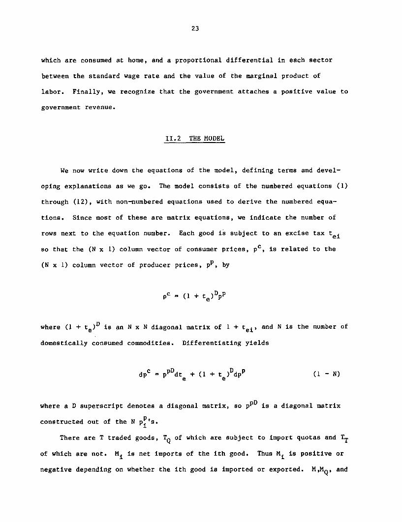
rows next to the equation number. Each good is subject to an excise tax tei
so that the (N x l) column vector of consumer prices, pc, is related to the
(N x 1) column vector of producer prices, pP, by
pc = (l + t )Dpp
where (I + t )D is an N x N diagonal matrix of 1 + tei, and N is the number of
domestically consumed commodities. Differentiating yields
dpc pPD dt + (1 + t )DdpP (I - N)e e
where a D superscript denotes a diagonal matrix, so ppD is a diagonal matrix
constructed out of the N ppis.i
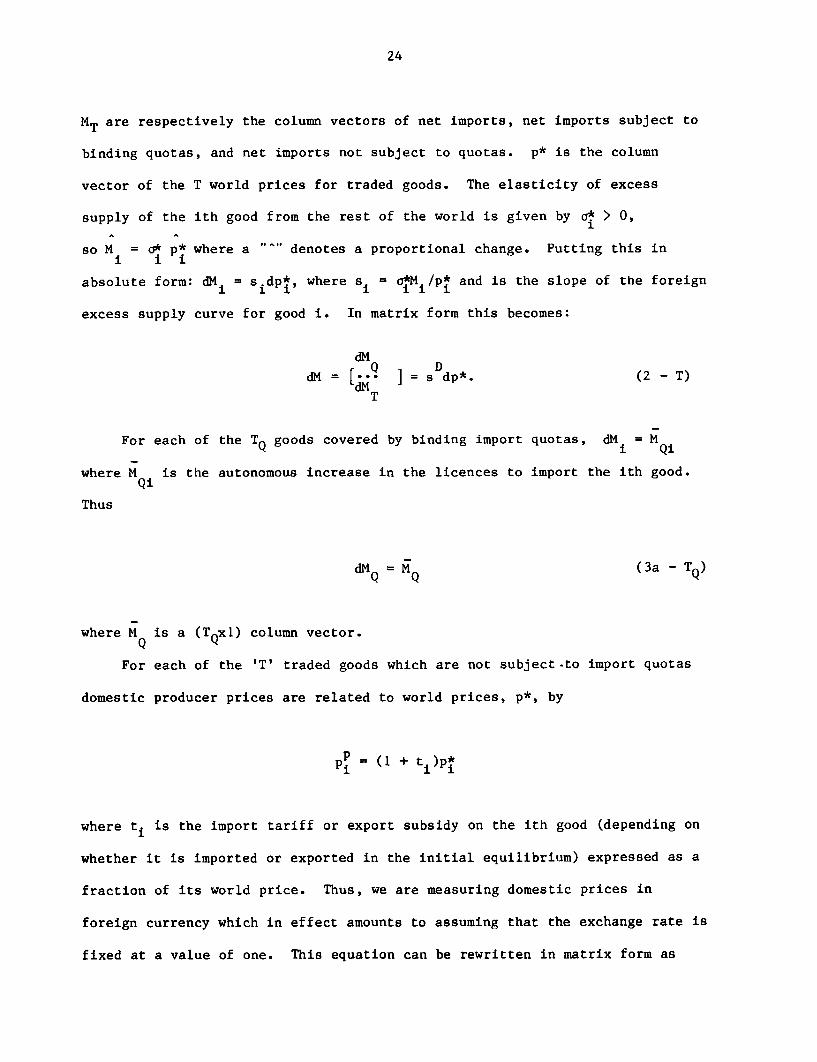
There are T traded goods, TQ of which are subject to import quotas and TT
of which are not. Mi is net imports of the ith good. Thus Mi is positive or
negative depending on whether the ith good is imported or exported. M,MQ. and
24
MT are respectively the column vectors of net imports, net imports subject to
binding quotas, and net imports not subject to quotas. p* is the column
vector of the T world prices for traded goods. The elasticity of excess
supply of the ith good from the rest of the world is given by O* > Q,i
so M = o* p* where a "" denotes a proportional change. Putting this ini i i
absolute form: dMi = s dp*, where s, = oM /p* and is the slope of the foreign
excess supply curve for good i. In matrix form this becomes:
dM
dM = [dM. ] = s dp*. (2 - T)dMT
For each of the TQ goods covered by binding import quotas, dM = M
where MQi is the autonomous increase in the licences to import the ith good.
Thus
dMQ= MQ (3a - TQ)
where M is a (TQxl) column vector.
For each of the 'T' traded goods which are not subject-to import quotas
domestic producer prices are related to world prices, p*, by
PP= (1+ ti)p*
where ti is the import tariff or export subsidy on the ith good (depending on
whether it is imported or exported in the initial equilibrium) expressed as a
fraction of its world price. Thus, we are measuring domestic prices in
foreign currency which in effect amounts to assuming that the exchange rate is
fixed at a value of one. This equation can be rewritten in matrix form as
25
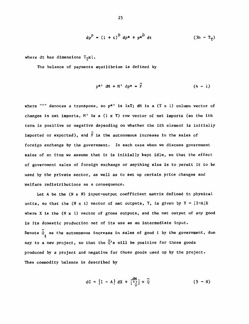
dpP = (1 + t)D dp* + p* dt (3b - TT)
where dt has dimensions TTxl.
The balance of payments equilibrium is defined by
p*' dM + M' dp* = F (4 - 1)
where ""' denotes a transpose, so p*' is lxT; dM is a (T x 1) column vector of
changes in net imports, M' is a (1 x T) row vector of net imports (so the ith
term is positive or negative depending on whether the ith element is initially
imported or exported), and F is the autonomous increase in the sales of
foreign exchange by the government. In each case when we discuss government
sales of an item we assume that it is initially kept idle, so that the effect
of government sales of foreign exchange or anything else is to permit it to be
used by the private sector, as well as to set up certain price changes and
welfare redistributions as a consequence.
Let A be the (N x N) input-output coefficient matrix defined in physical
units, so that the (N x 1) vector of net outputs, Y, is given by Y = [I-A]X
where X is the (N x 1) vector of gross outputs, and the net output of any good
is its domestic production net of its use as an intermediate input.
Denote Qi as the autonomous increase in sales of good i by the government, due
say to a new project, so that the Q's will be positive for those goods
produced by a project and negative for those goods used up by the project.
Then commodity balance is described by
dC = [I - A] dX + [d] + Q (5 - N)
26
where C is an (N x 1) vector of domestic consumption of the N goods, Q is the
(N x 1) vector of Qi's, and 0 is a column vector of zeros, one for each of the
non-tradeables.
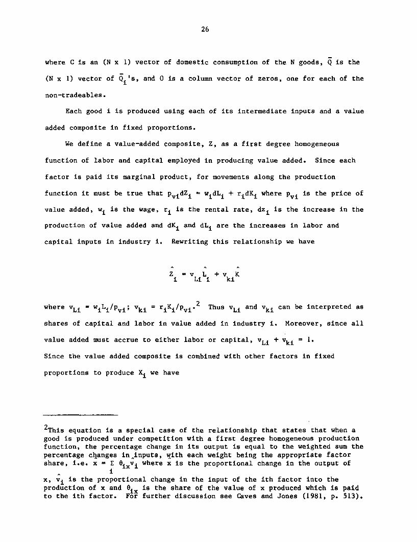
Each good i is produced using each of its intermediate inputs and a value
added composite in fixed proportions.
We define a value-added composite, Z, as a first degree homogeneous
function of labor and capital employed in producing value added. Since each
factor is paid its marginal product, for movements along the production
function it must be true that pvidZi , widLi + ridKi where pvi is the price of
value added, wi is the wage, ri is the rental rate, dzi is the increase in the
production of value added and dKi and dLi are the increases in labor and
capital inputs in industry i. Rewriting this relationship we have
Z = v L + v Ki Li i ki
where vLi =wiLi/pvi; Vki = riKi/pvi.2 Thus vLi and vki can be interpreted as
shares of capital and labor in value added in industry i. Moreover, since all
value added must accrue to either labor or capital, vLi + vki 1.
Since the value added composite is combined with other factors in fixed
proportions to produce Xi we have
2This equation is a special case of the relationship that states that when agood is produced under competition with a first degree homogeneous productionfunction, the percentage change in its output is equal to the weighted sum thepercentage chlanges in.inputs, with each weight being the appropriate factorshare, i.e. x = z 8ixvi where x is the proportional change in the output of
x, vi is the proportional change in the input of the ith factor into theproduction of x and ix is the share of the value of x produced which is paidto the ith factor. For further discussion see Caves and Jones (1981, p. 513).
27
Z iX
where Xi is the number of units of good i produced.
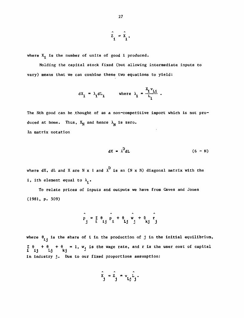
Holding the capital stock fixed (but allowing intermediate inputs to
vary) means that we can combine these two equations to yield:
XivLdXi = AidLi where Ai Li
i
The Nth good can be thought of as a non-competitive import which is not pro-
duced at home. Thus, XN and hence AN is zero.
In matrix notation
dX = A dL (6 - N)
where dX, dL and X are N x I and AD is an (N x N) diagonal matrix with the
i, ith element equal to Xi.
To relate prices of inputs and outputs we have from Caves and Jones
(1981, p. 509)
p = e p + 0 w + 0 rj i ij i Lj j kj j
where eij is the share of i in the production of j in the initial equilibrium,
E 6 + 6 + 0 = 1, w is the wage rate, and r is the user cost of capitali ij Lj kj Jin industry J. Due to our fixed proportions assumption:
X = Z v L.J J LiJj
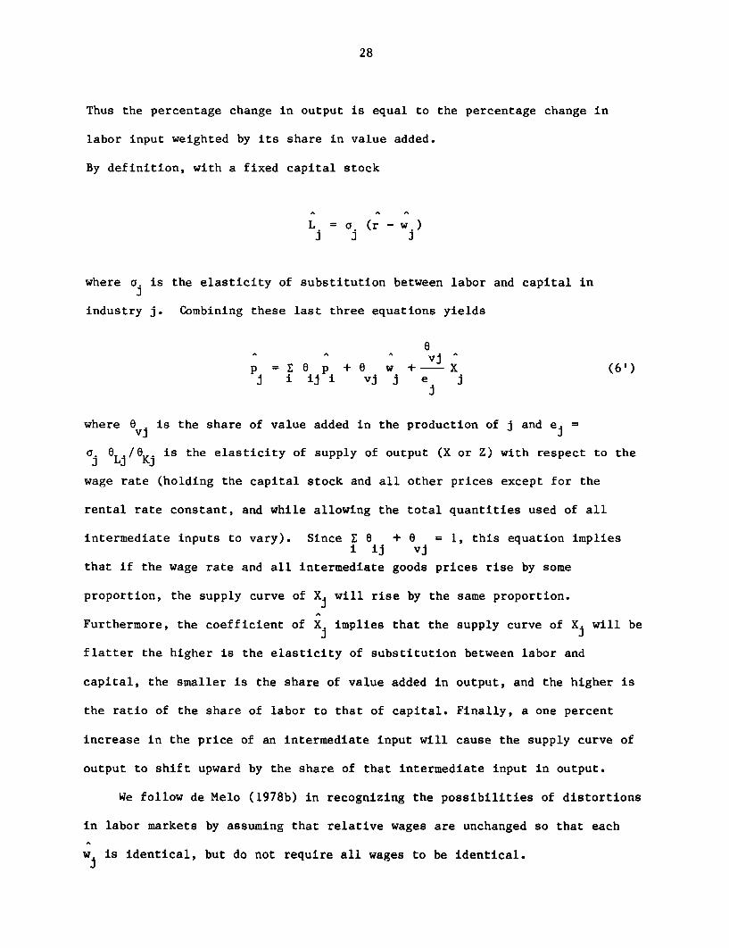
28
Thus the percentage change in output is equal to the percentage change in
labor input weighted by its share in value added.
By definition, with a fixed capital stock
L =a (r - w)
where a. is the elasticity of substitution between labor and capital in
industry j. Combining these last three equations yields
0A A A vi; (6'p = 6 p + e w + - X (6')j i ij i vj ; e j
where e0j is the share of value added in the production of j and ej =
aj 0 iK is the elasticity of supply of output (X or Z) with respect to the
wage rate (holding the capital stock and all other prices except for the
rental rate constant, and while allowing the total quantities used of all
intermediate inputs to vary). Since Z 0 + 0 = 1, this equation impliesi ij v;
that if the wage rate and all intermediate goods prices rise by some
proportion, the supply curve of X will rise by the same proportion.
Furthermore, the coefficient of Xi implies that the supply curve of X will be
flatter the higher is the elasticity of substitution between labor and
capital, the smaller is the share of value added in output, and the higher is
the ratio of the share of labor to that of capital. Finally, a one percent
increase in the price of an intermediate input will cause the supply curve of
output to shift upward by the share of that intermediate input in output.
We follow de Melo (1978b) in recognizing the possibilities of distortions
in labor markets by assuming that relative wages are unchanged so that each
w is identical, but do not require all wages to be identical.
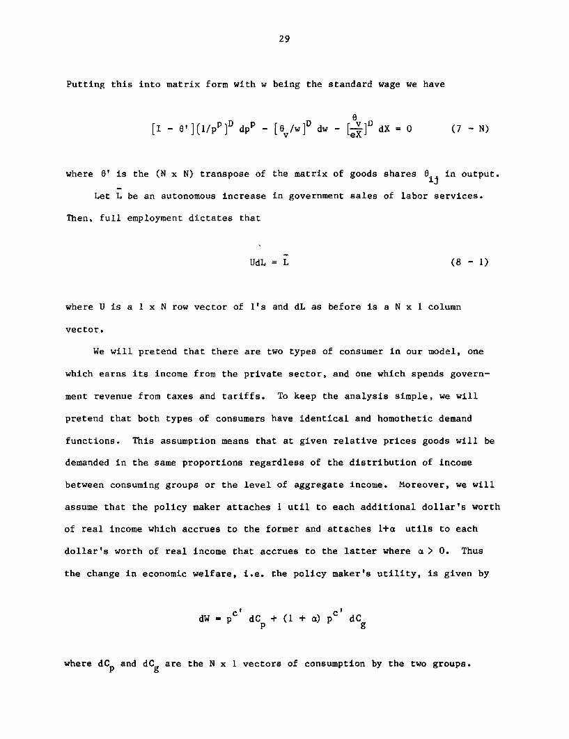
29
Putting this into matrix form with w being the standard wage we have
[I _ t]( 1/pP) dpP [v /w]D dw - [v 1D dX = - N)
where 0' is the (N x N) transpose of the matrix of goods shares 0ij in output.
Let L be an autonomous increase in government sales of labor services.
Then, full employment dictates that
UdL = L (8 - 1)
where U is a 1 x N row vector of l's and dL as before is a N x 1 column
vector.
We will pretend that there are two types of consumer in our model, one
which earns its income from the private sector, and one which spends govern-
ment revenue from taxes and tariffs. To keep the analysis simple, we will
pretend that both types of consumers have identical and homothetic demand
functions. This assumption means that at given relative prices goods will be
demanded in the same proportions regardless of the distribution of income
between consuming groups or the level of aggregate income. Moreover, we will
assume that the policy maker attaches 1 util to each additional dollar's worth
of real income which accrues to the former and attaches l+a utils to each
dollar's worth of real income that accrues to the latter where a > 0. Thus
the change in economic welfare, i.e. the policy maker's utility, is given by
dW = pc dC + (1 + a) pc dCp g
where dC and dC9 are the N x 1 vectors of consumption by the two groups.
30
Thus we are assuming that the policy maker trusts each consumer to allocate
his own budget to maximize utility and that the policy maker attaches a
premium of 100.a% to expenditure out of government revenue. Alternatively we
could have assumed that the government spends its revenue directly on public
goods and that the policy maker's welfare is the sum of utility accruing to
consumers, if we further assume that all consumers attach I util to a marginal
dollar spent on any private good and 1 + a utils to a marginal dollar spent on
any public good, where Cp and Cg are the vectors of consumption of private and
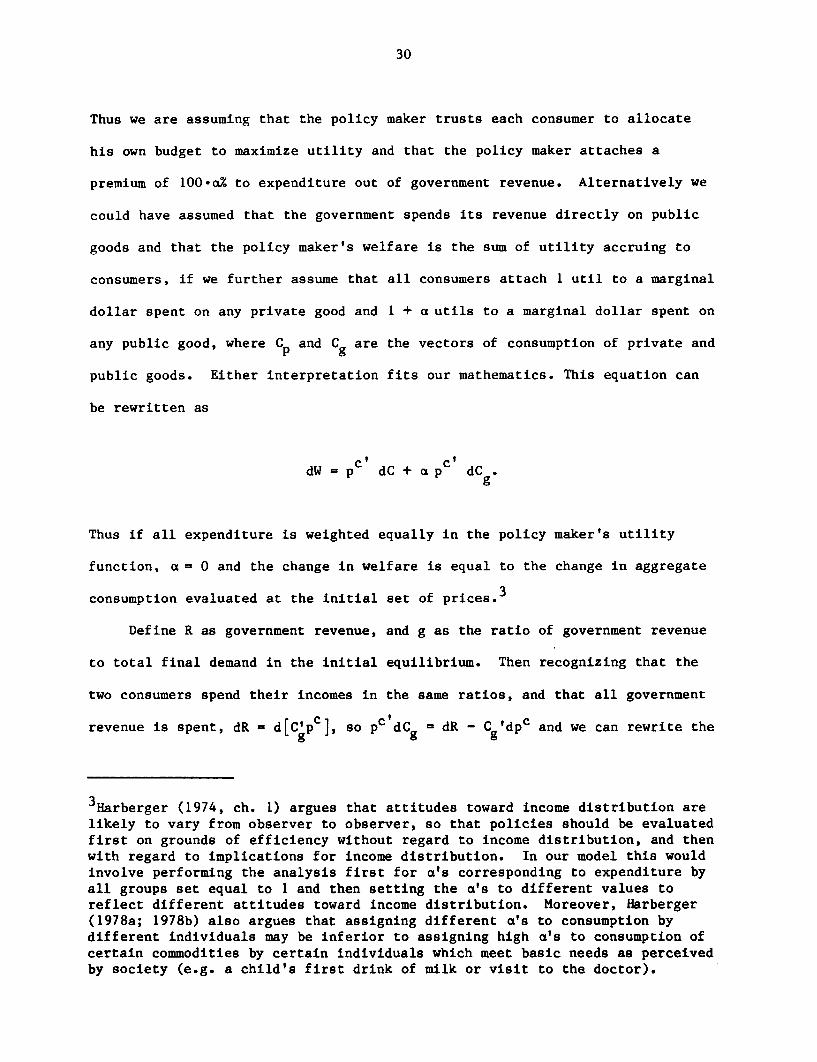
public goods. Either interpretation fits our mathematics. This equation can
be rewritten as
c' c'dW = p dC + a p dC.
Thus if all expenditure is weighted equally in the policy maker's utility
function, a = 0 and the change in welfare is equal to the change in aggregate
consumption evaluated at the initial set of prices.3
Define R as government revenue, and g as the ratio of government revenue
to total final demand in the initial equilibrium. Then recognizing that the
two consumers spend their incomes in the same ratios, and that all government
revenue is spent, dR = d[Cgpc], so pcdCg = dR - Cg dpc and we can rewrite the
3Harberger (1974, ch. 1) argues that attitudes toward income distribution arelikely to vary from observer to observer, so that policies should be evaluatedfirst on grounds of efficiency without regard to income distribution, and thenwith regard to implications for income distribution. In our model this wouldinvolve performing the analysis first for a's corresponding to expenditure byall groups set equal to 1 and then setting the a's to different values toreflect different attitudes toward income distribution. Moreover, Harberger(1978a; 1978b) also argues that assigning different a's to consumption bydifferent individuals may be inferior to assigning high a's to consumption ofcertain commodities by certain individuals which meet basic needs as perceivedby society (e.g. a child's first drink of milk or visit to the doctor).
31
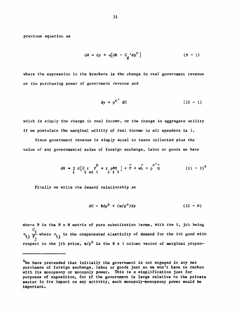
previous equation as
dW = dy + a[dR - Cg dpc] (9 - 1)
where the expression in the brackets is the change in real government revenue
or the purchasing power of government revenue and
dy = p dC (10 - 1)
which is simply the change in real income, or the change in aggregate utility
if we postulate the marginal utility of real income to all spenders is 1.
Since government revenue is simply equal to taxes collected plus the
value of any governmental sales of foreign exchange, labor or goods we have
dR = i d[C t P + t P*M ] + F + wL + p Q (11 -i i ei i ii i
Finally we write the demand relationship as
dC = Bdpc + (m/pC)dy (12 - N)
where B is the N x N matrix of pure substitution terms, with the i, jth being
lij p where nij is the compensated elasticity of demand for the ith good with
respect to the jth price, m/pc is the N x 1 column vector of marginal propen-
4We have pretended that initially the government is not engaged in any netpurchases of foreign exchange, labor or goods just so we won't have to reckonwith its monopsony or monopoly power. This is a simplification just forpurposes of exposition, for if the government is large relative to the privatesector in its impact on any activity, such monopoly-monopsony power would beimportant.
32
sities to consume out of real income and dy is the change in real income.
Since all output is consumed, and there is no money illusion, E n = 0 forj ij
all i.
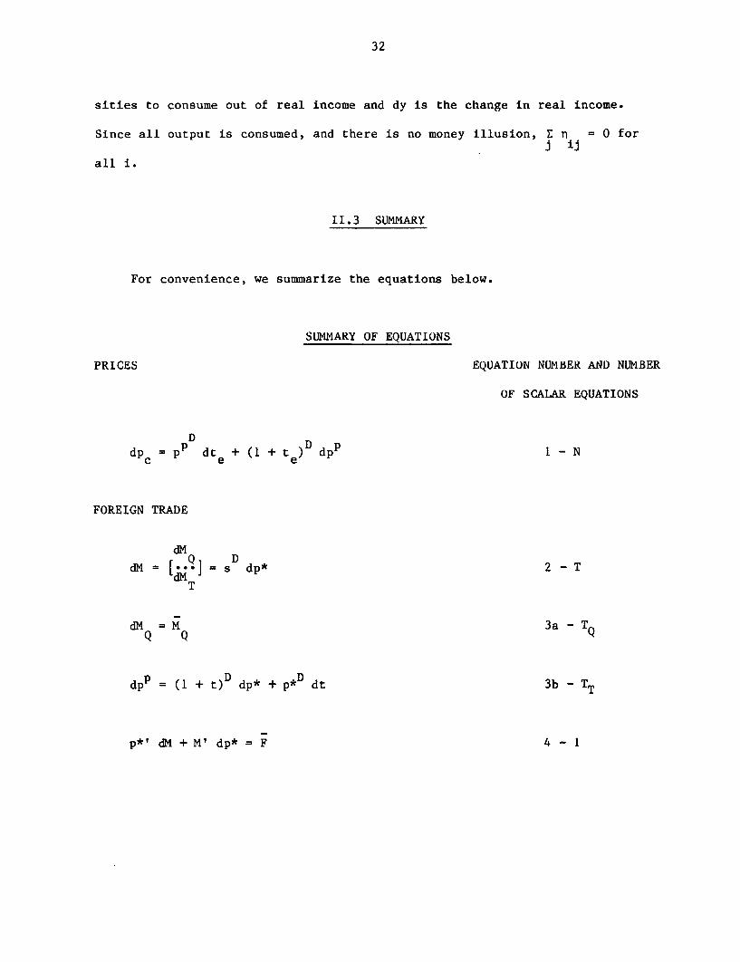
II.3 SUMMARY
For convenience, we summarize the equations below.
SUMMARY OF EQUATIONS
PRICES EQUATION NUMBER AND NUMBER
OF SCALAR EQUATIONS
DD pdpc = pP dte + (1 + te) dp 1 - N
FOREIGN TRADE
dM
dM = [..] = s dp* 2 - TdMT
dM =M 3a - TQ
dpP -(1 + t)D dp* + p* dt 3b - TT
p*1 dM + M' dp* = F 4 - 1
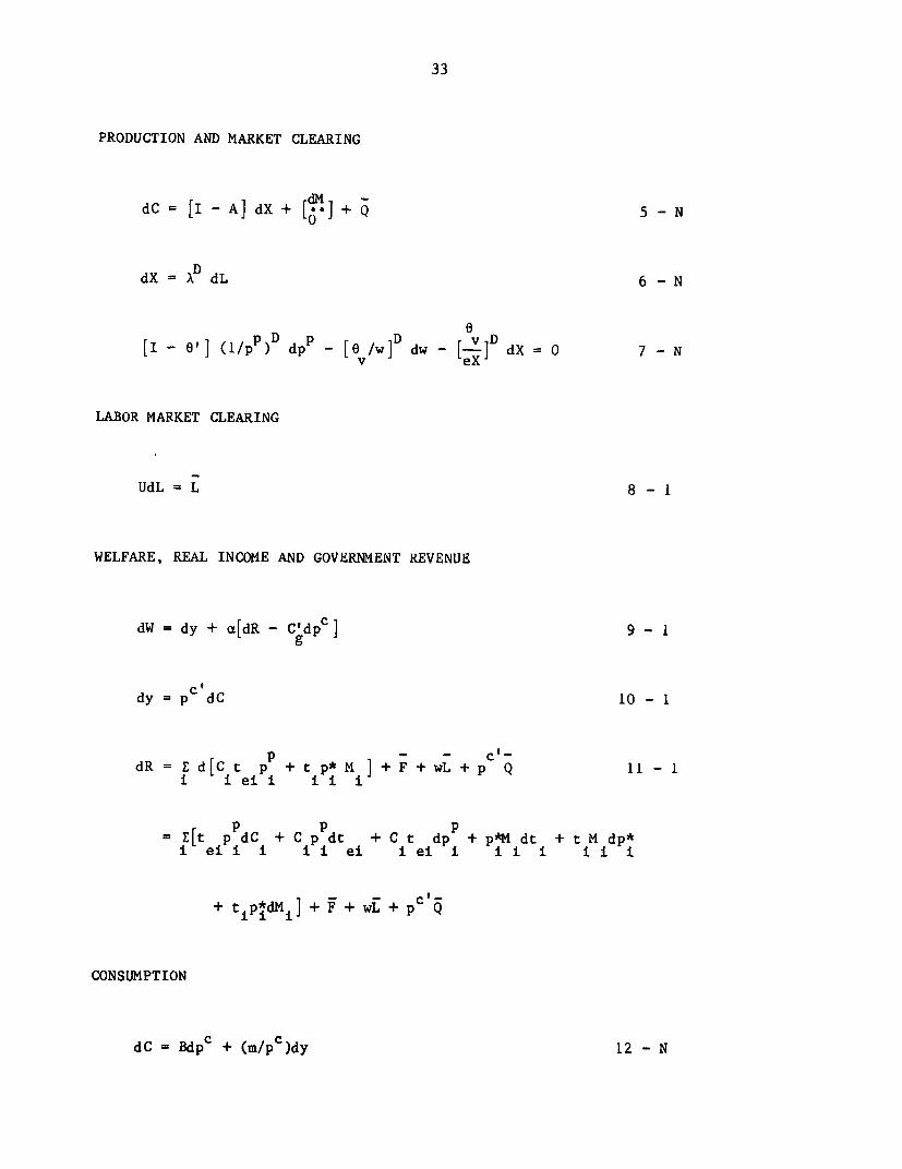
33
PRODUCTION AND MARKET CLEARING
dC = [I - A] dX + [O] + Q 5 - N
dX = ? dL 6 - N
6. 1 pD - e D - VD [I - e'] (1/p ) dpP _ [6 /w] dw V] dX 0 7 - N
LABOR MARKET CLEARING
UdL = L 8 -1
WELFARE, REAL INCOME AND GOVERNMENT REVENUE
dW = dy + a[dR - Cgdp'] 9 -1g
dy = p dC 10- 1
p . - Cl-dR = E d [ t P + tPd* Mi] + F + wL + p Q 11 - 1
i i ei i i i i
= Etp pdC + C pdt + Ct dpp + p*M dt + tM dp*i ei i i i i ei i ei i i i i i i i
+ t p*idMi] + F + wE + p &
CONSUMPTION
dC = BdpC + (m/pc)dy 12 - N
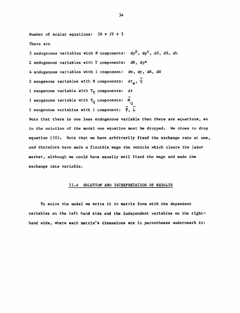
34
Number of scalar equations: 5N + 2T + 5
There are
5 endogenous variables with N components: dpp, dpC, dC, dX, dL
2 endogenous variables with T components: dM, dp*
4 endogenous variables with 1 component: dw, dy, dR, dW
2 exogenous variables with N components: dte9 Q
1 exogenous variable with TT components: dt
I exogenous variable with TQ components: M
2 exogenous variables with 1 component: F, L
Note that there is one less endogenous variable than there are equations, so
in the solution of the model one equation must be dropped. We chose to drop
equation (10). Note that we have arbitrarily fixed the exchange rate at one,
and therefore have made a flexible wage the vehicle which clears the labor
market, although we could have equally well fixed the wage and made the
exchange rate variable.
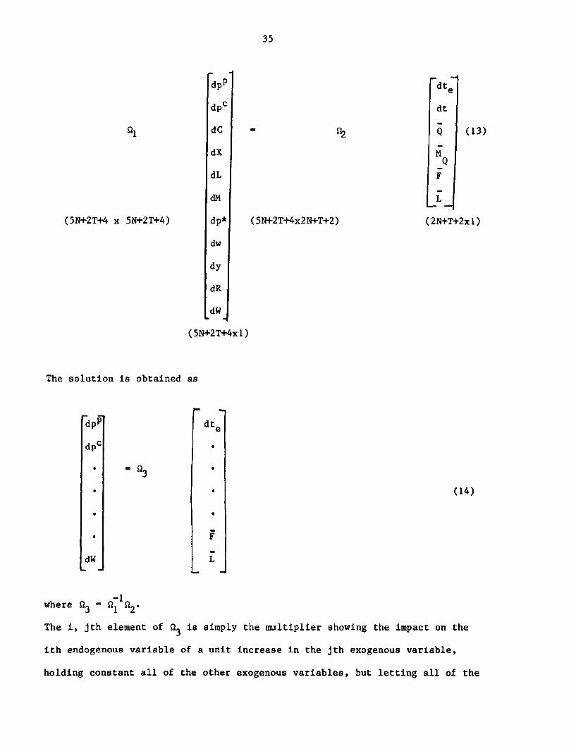
II.4 SOLUTION AND INTERPRETATION OF RESULTS
To solve the model we write it in matrix form with the dependent
variables on the left hand side and the independent variables on the right-
hand side, where each matrix's dimensions are in parentheses underneath it:
35
dpP dte
dpC dt
Q1 dC = Q (13)
dX 14-Q
dL F
&I LL
(5N+2T+4 x 5N+2T+4) dp* (5N+2T+4x2N+T+2) (2N+T+2xl)
dw
dy
dR
dW
(5N+2T+4xl)
The solution is obtained as
dpp dte
dpC
* * ~~~~~~~~~~~~~~~~(14)
dW L
where Q3= n1Q2
The i, jth element of Q3 is simply the multiplier showing the impact on the
ith endogenous variable of a unit increase in the jth exogenous variable,
holding constant all of the other exogenous variables, but letting all of the
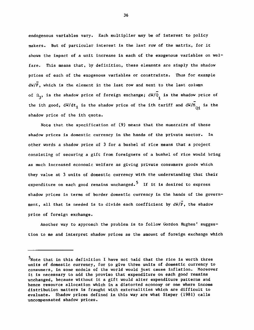
36
endogenous variables vary. Each multiplier may be of interest to policy
makers. But of particular interest is the last row of the matrix, for it
shows the impact of a unit increase in each of the exogenous variables on wel-
fare. This means that, by definition, these elements are simply the shadow
prices of each of the exogenous variables or constraints. Thus for example
dW/F, which is the element in the last row and next to the last column
of S3, is the shadow price of foreign exchange; dW/Q is the shadow price of
the ith good, dW/dti is the shadow price of the ith tariff and dW/MQi is the
shadow price of the ith quota.
Note that the specification of (9) means that the numeraire of these
shadow prices is domestic currency in the hands of the private sector. In
other words a shadow price of 3 for a bushel of rice means that a project
consisting of securing a gift from foreigners of a bushel of rice would bring
as much increased economic welfare as giving private consumers goods which
they value at 3 units Qf domestic currency with the understanding that their
expenditure on each good remains unchanged.5 If it is desired to express
shadow prices in terms of border domestic currency in the hands of the govern-
ment, all that is needed is to divide each coefficient by dW/F, the shadow
price of foreign exchange.
Another way to approach the problem is to follow Gordon Hughes' sugges-
tion to me and interpret shadow prices as the amount of foreign exchange which
5Note that in this definition I have not said that the rice is worth threeunits of domestic currency, for to give three units of domestic currency toconsumers, in some models of the world would just cause inflation. Moreoverit is necessary to add the proviso that expenditure on each good remainsunchanged, because without it a gift would alter expenditure patterns andhence resource allocation which in a distorted economy or one where incomedistribution matters is fraught with externalities which are difficult toevaluate. Shadow prices defined in this way are what Sieper (1981) callsuncompensated shadow prices.
37
the government would have to buy back from the economy in return for govern-
ment sale of one unit of the commodity or factor in question in order to leave
welfare unchanged. This is the Little-Mirrlees approach which consists of
measuring the shadow price of anything by its "foreign exchange equivalent." 6
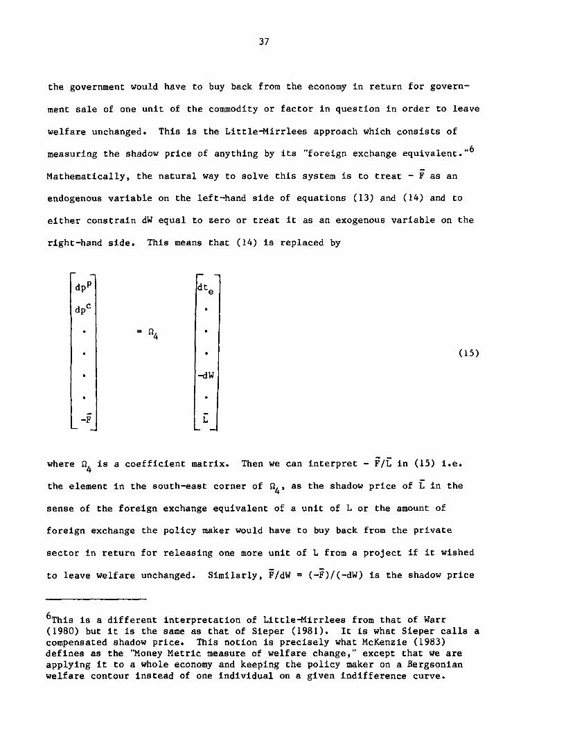
Mathematically, the natural way to solve this system is to treat - F as an
endogenous variable on the left-hand side of equations (13) and (14) and to
either constrain dW equal to zero or treat it as an exogenous variable on the
right-hand side. This means that (14) is replaced by
dpP dte
dpC
4
* ~~~~~-dW
4
where 4 is a coefficient matrix. Then we can interpret - FIE in (15) i.e.
the element in the south-east corner of f4, as the shadow price of L in the
sense of the foreign exchange equivalent of a unit of L or the amount of
foreign exchange the policy maker would have to buy back from the private
sector in return for releasing one more unit of L from a project if it wished
to leave welfare unchanged. Similarly, F/dW = (-F)/(-dW) is the shadow price
6This is a different interpretation of Little-Mirrlees from that of Warr(1980) but it is the same as that of Sieper (1981). It is what Sieper calls acompensated shadow price. This notion is precisely what McKenzie (1983)defines as the "Money Metric measure of welfare change," except that we areapplying it to a whole economy and keeping the policy maker on a Bergsonianwelfare contour instead of one individual on a given indifference curve.
38
of economic welfare, in the sense that it indicates how much foreign exchange
in the hands of the private sector would be needed to generate one more unit
of economic welfare. The reciprocal of this term is what Warr (1980, p. 34)
refers to as "the shadow price of foreign exchange in utility numeraire" and
what Bacha and Taylor (1971) refer to as the second best shadow price of
foreign exchange.
One of the nice aspects of this approach is that it brings out the logi-
cal relationship between determining the desirability of a particular policy
reform (e.g. a package of adjustments in tariffs, quotas and excise taxes) and
a particular project (e.g. a package of positive excess supplies of certain
goods [outputs] and negative excess supplies of certain others [inputs]). In
both cases the desirability of the package is evaluated by multiplying the
package of changes by the shadow price attached to each change.
Moreover, in some circumstances it may be important to have consistent
estimates of both shadow prices of policy parameters and goods. For example,
suppose that a particular project involves the production of certain goods
along with the use of certain inputs and the relaxation of certain import
quotas, but the raising of certain tariffs in order to leave government
revenue unchanged. Evaluation of the desirability of this project will
involve evaluating the change in all of these variables by multiplying the
various changes by the appropriate shadow prices. Such an exercise would be
facilitated by the approach laid out here, both because our matrix can be used
to calculate the shadow price of each constraint and good, and because the
revenue row can be used to determine the contribution of each change in
inputs, outputs and constraints to revenue, thereby enabling one to calculate
the change in the tariff or tariffs that would just offset the negative
revenue effects of the project itself.
39
A few more additional points are worth making:
A. Suppose we wish to know how free trade will affect equilibrium. We can
express all quantitative constraints on trade as a tariff equivalent, and then
solve the model for a small equiproportional cut in all tariffs. The model
should give very accurate estimates for a uniform tariff reduction as small as
1%. Then all we need to do to have a measure of the impact of free trade is
to multiply the multipliers for a 1% uniform cut in tariffs by 100. Such a
measure will be an imperfect estimate, but it should give a reasonably accu-
rate ranking of industries from most hurt to least hurt. For a more precise
figure one could apply the n step procedure described in DPSV (1982, sec. 8,
ch. 5 and sec. 47).
B. Suppose we wish to calculate net effective protection or domestic resource
cost. Once a general equilibrium program is set up, it would be a small
additional programing problem to pull out of it standard measures of net ERPs
and DRCs. Moreover if one wishes to use the effective rate of protection as a
measure of the effect of the tariff structure on resource allocation, it seems
to me that neither the Corden nor the Balassa way of handling non-traded goods
nor the Balassa method for handling exchange rate change is as good as the
following: Use the linearized general equilibrium model as described above to
estimate changes in wage rates, exchange rates and non-traded goods prices,
and then use these to calculate net effective protection.7 Similarly use the
model to calculate shadow prices for inputs into a project and outputs from
it. Then combining input and output flows from a hypothetical project enables
us to calculate its DRC.
7For definitions of these methods and the formulas see Balassa and Associates(1982, pp. 352-354). This way of dealing with non-traded goods is what Ray(1973) proposes and labels the Scott method after Little, Scitovsky and Scott(1970, p. 432).
40
Also, as Garry Pursell has suggested, one may want net effective protec-
tion statistics on a more disaggregated basis than could be estimated using a
general equilibrium model. In this case, one could use the linearized general
equilibrium model to calculate price changes for various input aggregates, and
use these in order to calculate more disaggregated net effective protection
measures.
C. The kind of analysis proposed here is not at conflict with the partial
equilibrium analyses provided by Corden (1974) and others. Their studies can
be interpreted as describing various aspects of a general equilibrium system
in isolation. It is the role of a model of the sort described here to provide
a framework for putting together the ideas Corden discussed separately in
various chapters, and treating them all together in a general framework.
Moreover, the techniques proposed here are well known and have been imple-
mented with varying degrees of complexity and disaggregation and to focus on
various issues.8
D. Now let us provide a measure of the welfare cost of all the distortions
taken together to a quadratic approximation. In order to avoid the problem of
varying marginal utility of income, we will interpret the welfare cost of an
existing set of distortions as the amount of foreign exchange which could be
taxed away from the economy, simultaneously with the distortion elimination so
as to leave domestic welfare unchanged. Thus, we are adopting the Little-
Mirrlees numeraire, and as our measure of welfare change, we are taking the
compensating variation in foreign exchange. To measure the welfare cost of
8See for example Taylor and Black (1974), the ORANI model described in DPSV(1982), Stoeckel (1978) which also deals with Australia and Baade andRichardson (1973), which deals with the United States and permits labor toacquire new skills in response to changed relative wages, as well as the earlywork by Johansen (1960).
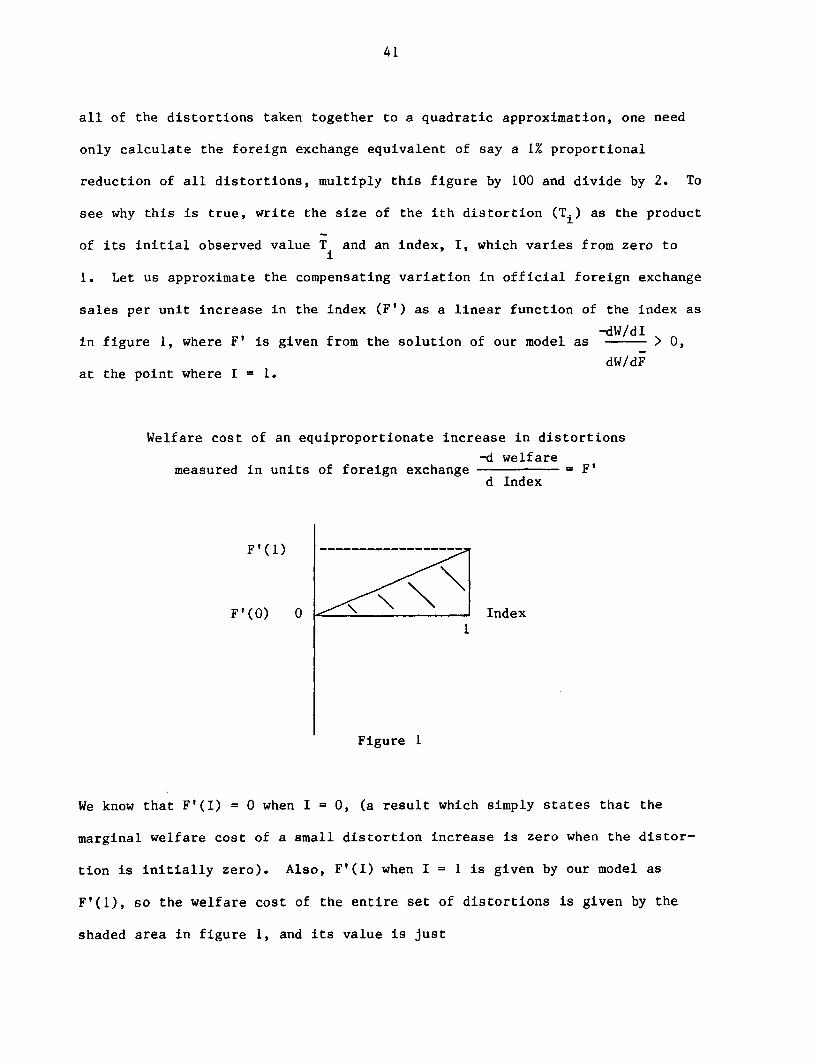
41
all of the distortions taken together to a quadratic approximation, one need
only calculate the foreign exchange equivalent of say a 1% proportional
reduction of all distortions, multiply this figure by 100 and divide by 2. To
see why this is true, write the size of the ith distortion (Ti) as the product
of its initial observed value Ti and an index, I, which varies from zero to
1. Let us approximate the compensating variation in official foreign exchange
sales per unit increase in the index (F') as a linear function of the index as
in figure 1, where F' is given from the solution of our model as -did > 0,
dW/dFat the point where I = 1.
Welfare cost of an equiproportionate increase in distortions
-d welfaremeasured in units of foreign exchange = F'
d Index
F'(0) 0 Index
Figure 1
We know that F'(I) = 0 when I = 0, (a result which simply states that the
marginal welfare cost of a small distortion increase is zero when the distor-
tion is initially zero). Also, F'(I) when I = 1 is given by our model as
F'(1), so the welfare cost of the entire set of distortions is given by the
shaded area in figure 1, and its value is just
42
F'(1) + F'(0) F'(1) + 0 F'(1)
2 2 2
Thus, if we discovered that a 1% cut in the initial level of each distortion
would increase national income by 1 million dollars, a complete elimination of
them should increase national income by 50 million dollars.
E. Now let us make explicit the mathematics that we are using in part D,
since this mathematics is also applied implicitly by Johnson (1971) in his
chapters involving consumers' surplus. Implicitly, we have expressed the
compensating variation in foreign exchange per unit change in the index as a
Taylor's series:
2dF F'(1) (I-1)Ft(1) (I-1) Ftt(1)dI 2
We assume that third and higher order terms are small relative to the first
and second order terms so that we can drop third and higher order terms.
Then, recognizing that solution of our model gives us F'(1) we solve for
F''(1) as
F'(0) = 0 = F'(1) + (0-1) F'"(1)
to yield
02
OdF 0 I F'(1) -F'(l)F= - dI f [F'(1) + (I-1) F'(1)]dl = =2 2
This is the measure we derived in the previous section and it simply states
that the variation in foreign exchange endowment which would just compensate
for the elimination of all distortions is -F'(1)/2 < 0. Thus, we can see that
43
our welfare approximation is accurate to the extent that it is legitimate to
approximate the compensating variation in foreign exchange as a second order
Taylor's series in the distortion index.
F. Note that once one has obtained either the curve in Figure 1 or else the
Taylor's series approximation, one could calculate the welfare effect of any
change in the distortion index. For example, a doubling of all tariffs and
taxes would carry with it a compensating variation of foreign exchange of
AF = [F'(1)/2][2 - 1] = 3F'(1)/2. Of course all of these approximations are
needed only if one wishes to avoid using the numerical integration techniques
described in DPSV (1982) or building a CGE model.
II.5 EXTENSIONS
In the model just described, we assumed that capital was sector specific
but that labor was perfectly mobile between sectors, and was homogeneous. We
also postulated that demand functions of individuals were identical and homo-
thetic. In this section we discuss alternative ways of modeling the economy.
The thrust of this section is that the linear modeling framework can be used
to describe a large range of models and adjustment mechanisms. The only
situation it can't handle is a world where the pattern of specialization is
uncertain, a problem which crops up when we have all four of the following
conditions together: There are no diseconomies of scale, all factors are
perfectly mobile, world prices are fixed, and there are more traded goods than
44
mobile factors.9 We now turn to particular aspects of economic systems which
might be worth modeling.
a. The Labor Market
We have assumed that the labor market clears, and that price changes keep
the balance of payments in equilibrium. There is no reason, though, why we
could not model a situation in which money wages or real wages are inflexible
downwards in a few or all sectors as DPSV (1982) describe. Moreover, we have
assumed that labor is paid its marginal product, but we could equally well
have modeled share cropping arrangements where labor is entitled to some
fraction of the output it produces.10 Also, we have postulated constant pro-
portional wage differentials between sectors, but there is no reason why that
too could not be variable,11 and then if we believe that the Harris-Todaro
mechanism is at work creating a throng of urban unemployed who accept
unemployment some of the time in return for being employed some of the time at
the higher urban wage (see Corden 1974, 144-54), we could model that unemploy-
ment (a la Corden) as being dependent on the wage differential.
Similarly, we could recognize that in many sectors wages may only be
partially flexible, with the rate of fall being a function of the amount of
90ne way of handling the problem is to follow de Melo (1978a; 1980) and otherscited there in postulating mildly decreasing returns to scale. De Melo postu-lates decreasing returns to scale of .9 in all sectors. As de Melo (1980,p. 115) notes, assuming that each industry employs a fixed factor specific toitself amounts to assuming diminishing returns to the other non-specificfactors. Thus, the model presented here contains many of the core elementswhich one would use in modeling a longer run time horizon with most factors ofproduction inter-sectorally mobile.
'OFor discussion of recent work on this problem, see C. L. G. Bell (1979).
lFor analysis of the long and short run effects of eliminating factor marketdistortions in Columbia see de Melo (1977).
45
unemployment in the sector in question.
b. The Exchange Rate
We have assumed the balance of payments to be in perpetual equilibrium.
But again we could have held certain internal prices as well as the exchange
rate fixed and permitted the balance of payments to vary.
c. Industrial Organization
We have assumed competition in product markets, but one could alterna-
tively use a model of mark up pricing following Staelin's (1976) analysis of
the Ivory Coast or Harris's (1982) analysis of Canada.
d. Private Sector Shadow Prices
So far, we have interpreted shadow prices of goods as the gain in social
welfare or government stocks of foreign exchange of governmental sale of one
unit of the good or factor. Sometimes the government is called upon to
evaluate a particular private sector project carried out by someone in a
particular category (e.g. small business, large business, or foreigner, etc.).
A project carried out by such a person is equivalent to the project being
carried out by the government combined with a transfer by the government to
the person of a sum of money equal to the project's cash flow. Thus the net
sale of a good or factor by such a person is equivalent to the same net sale
by the government combined with a net transfer by the government to the person
equal to the market value of the good or factor. Thus the shadow price of a
good produced or consumed by a private sector project should equal the shadow
price as previously calculated plus the shadow price of a transfer from the
government to the particular person (which will generally be negative).
46
Therefore, if the individual is a particularly worthy soul in the eyes of the
government, the government will put only a slightly negative shadow price on
transfers of revenues from him. Thus it will attach a high shadow price to
both commodities he uses and commodities he produces, and if the individual
anticipates a profit from the activity, the government should be more likely
to approve the activity than if a "less worthy" soul proposes to undertake it.
If it is possible to reform only some aspects of the tax code, those
aspects which are reformable should be modified so that producers and
consumers in effect respond to shadow prices rather than market prices. The
easiest scheme would probably be to publish a common set of shadow prices for
each input and output for all firms and levy taxes or subsidies as needed to
bring after tax or subsidy market prices in line with shadow prices and then
to tax any profits that are left at a rate appropriate to the category of the
individual proprietor. Such an approach would be the appropriate way to
modify investment codes.
In many cases there are taxes that the government could levy without
incurring any efficiency cost at all, such as auctioning of import licenses.
If those kinds of taxes are available and it is politically feasible to levy
them, it seems hard to justify placing a significant premium on government
revenue. Similarly, there may be reasonably efficient taxes that one could
levy on the rich. In the limit as revenue collection and income redistribu-
tion becomes costless, we do not need to distinguish between shadow prices to
the government and the private sector, which simplifies the analysis consider-
ably, for in that case, the shadow price of any good or factor simply becomes
the welfare impact of an increase in the economy's endowment of that good or
factor. This is the approach we use in subsequent chapters.
47
e. Heterogeneous Labor
We have assumed that all labor is homogeneous. But there is no reason
why we could not recognize that labor is heterogeneous in skills, aptitudes
and tastes. Then we could make output in each sector depend on the employment
of various types of labor, with whatever degree of substitution between them
seems appropriate (on this see DPSV 1982, pp. 76-90). Then on the supply
side, we could recognize that labor's willingness to switch industries or to
acquire new skills depends on relative wages. We could even have voluntary
unemployment and make it dependent on the real wage, and the level of
unemployment compensation. Baade and Richardson (1973) have treated labor in
this way.
f. Sectorally Mobile Capital
One could also deal with mobile capital in a similar way. We cannot let
all factors which are used in producing tradeable goods be perfectly mobile,
for then the problem of specialization arises. But we can recognize that as
differentials between rates of return to capital in different sectors
increase, increasing amounts of capital will move from the low return sectors
to the high return ones. We can then relate changes in capital allocation to
changes in real rates of return with a matrix of transition coefficients, much
as Baade and Richardson (1973) did for labor. If one is building a model to
describe the short run, one would want the transition coefficients showing the
responsiveness of capital's location to rental differentials to be small, but
if one is building a model to describe a longer time horizon, one would want
somewhat larger coefficients. Such a scheme is discussed by DPSV (1982, pp.
118-122).
48
g. Savings
When modeling a still longer time horizon over which savings can take
place, one might wish to make the aggregate supply of capital responsive to
the rate of return, government revenue or the incomes of certain groups. If
each industry produced output using a fixed factor plus variable factors, one
could simply assume that capital is allocated so as to equalize rates of
return in all industries. Otherwise, in order to avoid the specialization
problem one would need to make some alternative assumption, for example by
assuming that new capital is allocated to industries in accordance with rates
of return and initial capital stocks, but that it is not allocated in such a
way that rates of return are equalized or else that there are either
decreasing returns to scale (de Melo 1978a; 1980) or that both domestic and
foreign demanders view domestic and foreign goods as imperfect substitutes, so
that both the foreign and domestic demands for domestically produced goods are
less than perfectly elastic (e.g. de Melo and Robinson (1981) and Dervis, de
Melo and Robinson (1981)).
h. Demand
We have assumed that within each category of goods domestic and foreign
products are perceived as identical by consumers and producers. However, the
standard assumption in computable General Equilibrium (CGE) modeling is to
postulate that both producers and consumers view domestic and foreign goods to
be imperfect substitutes, an assumption that DPSV (1982) have used in this
sort of modeling as well. Finally, we have assumed that all consumers have
identical demand patterns, but there is no reason why we could not introduce
different behavior by different consumer groups who derive their incomes from
different sources.
49
i. Data
While data requirements would depend on the precise use and level of
sophistication which one would like to put models of this sort to, in order to
apply the model developed in this chapter one needs only know the input-output
flows in the base year combined with tariffs, taxes, and quotas, figures
showing how value added is broken down into returns to land, capital and labor
and have guesses about what income elasticities and elasticities of substitu-
tion in production and consumption are. For a discussion of data requirements
of a sophisticated linear model see chapter 4 of DPSV (1982), "The ORANI data
input files."
j. How Complex?
Calibrating models of this sort can take as much or as little energy as
the user wishes. Much use could be made of very simple models with one
exportable, one importable and one nontradeable. Also, one can either collect
detailed data or just simply assume that many parameter values are very
similar to those of other countries and ask knowledgeable country experts to
provide the rest based on their best guesses about how the economy in question
works. Then one can use a model of this sort to work out the consequences of
various changes in endowments, policy parameters or exogenously given
circumstances. On the other hand if one wishes to use a model of this sort
for detailed sectoral planning, one would wish to use a highly disaggregated
model with very careful specification of behavior patterns, and such a task
could be very expensive and fraught with both conceptual difficulties and data
problems that would require considerable hard work and ingenuity to solve.
For further work on how complex linear models have been constructed, and
the uses they have been put to both in the narrow sense of what has been

50
simulated and in the more general sense of what their impact has been in the
policy making context, see DPSV (1982). Now we consider in Chapter III the
other extreme, namely some applications of quite simple models.

51
Chapter III
APPLICATIONS TO SECOND BEST TARIFFS
III.1 ON A QUICK AND SIMPLE APPROACH TO
ESTIMATING SECOND BEST TARIFFS
l.a Introduction
Now that we have constructed a reasonably detailed model and explored its
implications, we turn to a succession of special cases. In this first section
of Chapter III, we discuss a simple procedure for determining second best
optimum tariffs and show how it could be useful in the policy advising
process. Policy advisors are frequently faced with a problem of the following
sort. Import tariffs on certain goods - typically final products - are fixed
by political considerations to be above some floor while subsidies on certain
exports are forced by factors such as the possibilities for invoice falsifica-
tion and smuggling not to exceed a certain ceiling. However, there are some
imports (perhaps intermediate products and raw materials) whose initial
tariffs are low and can be raised without facing political opposition. The
problem is, what sort of tariff level should the policy advisor recommend on
these goods.
More generally, and in the jargon of economics, suppose a policy advisor
faces many distortions and only has a few policy tools to cope with them. How
should he set the levels of these tools?
A second problem facing the policy advisor is that he must arm policy
makers with policy analysis which is both believable and comprehensible: the

52
models used must incorporate enough of the policy maker's beliefs about how
his economy works so that he believes the models are worth using and they must
be sufficiently clear and simple so that policy makers understand them well
enough so as to convince others that the recommendations which flow from them
should be implemented. To cope with this problem we need to employ in the
policy process simple models which are easy for local policy makers to under-
stand, in which the basic economic principles are clear, and which can
profitably employ information from the policy makers for their actual
implementation.
In this section we develop an approach to the problem noted in the first
paragraph which has the benefits cited in the third. Rather than develop a
full-blown detailed model, we present a simple model, and then indicate how it
can be extended. The economics here is not new, but I believe the approach to
policy advice is.
1.b Consumption and Welfare
Throughout this section, we assume that all final demand is consumption;
we ignore income-distribution considerations and we assume that consumers know
what is good for them; hence private utility is synonymous with social
utility. In other words Chapter II's a is equal to zero. We assume away all
externality, assume our economy trades at fixed world prices and postulate an
import tax or export subsidy equal to ti levied on the world price of good
i. Should we have an import subsidy or an export tax levied on the good, ti
would be negative. Since we assume that no good will be both imported and
exported ti will be interpreted as referring to imports or exports of good i
depending on whether in the equilibrium considered the good is imported or
53
exported. ti is assumed to be expressed as a fraction of the foreign price.
In what follows:
*Pi is the world price of good i
Pi is the domestic price of good i
Qi is the net domestic output of good i. Thus Qi<O implies that the
economy uses more i as an intermediate input than it produces as
gross output.
Ei is net export of good i.
Finally, pi will be taken to be the C.I.F. price of good i if it is an import
and the F.O.B. price of good i if it is an export in the initial equilibrium.
We define the marginal utility of income as unity in the neighborhood of
the initial equilibrium, and since consumers are assumed to know what is good
for them, the change in society's utility, dy, evaluated at prices to
consumers is given by
dy = E p dC (1)
i
where Ci is consumption of the ith good and dCi is its change. Thus, if we
knew how consumption of each and every good would be affected by a change in
tariffs, we could evaluate the utility associated with that change solely by
reference to equation (1).
I.c Production, Trade and Welfare
Suppose instead we had information on the dQ's and dE's. Then we could
calculate the dC's and proceed as before. However, suppose we have informa-
tion on the dQ's and the dE's, along with information on tariffs, but no
direct information on prices. Let's see how to use that information to calcu-
late the utility of a tariff change.

54
The balance of payments constraint means that
* *E p dE = (p -p )dE + E p dE =0. (2)iii i i i i ii
The fact that the economy is on its production possibilities frontier means
that
E p dQ a0. (3)i ii
Combining (1), (2) and (3) with the fact that dCi = dQi - dEi implies
*dy = E(p -p ) dE . (4)
ii i i
Since the taxes and tariffs are the wedges between buyer and seller, we can
reexpress (4) as*
dy = -Z t p dE . (5)i ii i
Now, suppose that all t's are fixed, except for to, and our problem is to find
the optimum level of to. A necessary condition for us to be at a welfare
optimum is that small changes in to leave y unchanged. Thus to will be at its
optimum level when
dEdy * i- = -E t p -= 0dt i i i dt
0 0
or whendE
i=N * iz t p -
i=1 i i dt
t* =o p*dE
0 0
dt0
55
where t* is the second-best optimum tariff on good 0, and there are N + 10
traded goods in the economy. What equation (6) tells us is that we can
calculate to by knowledge of how trade flows depend on the tariff on the0
zeroth commodity plus the existing levels of other tariffs and subsidies to
trade. We turn now to two applications of this formula.
I.d One Import and One Export
Suppose our economy imports good "1" and exports good O", and engages in
no other trade. Furthermore, suppose the import tariff on "1 is given, and
we need to determine the optimum tax or subsidy on the export of good "O".
Since trade is always balanced
* *
p dE P1 dE1o o- + = 0,dt dt
0 0
i.e. any change in imports must be balanced by an equal change in exports.
Thus, (6) tells that
t* = tl. (7)0
In other words the import tariff on good 1 must be matched by an equal subsidy
on the export of good 0. This conclusion is of course familiar from the
Lerner neutrality theorem,1 which states that a common import tariff on all
imports which is matched by a common export subsidy on all exports has no
economic effect. Note that in applying this formula our policy maker is
reminded that exchange rates or relative prices will always be forced to
1For a discussion of this theorem, see Kaempfer and Tower (1982).
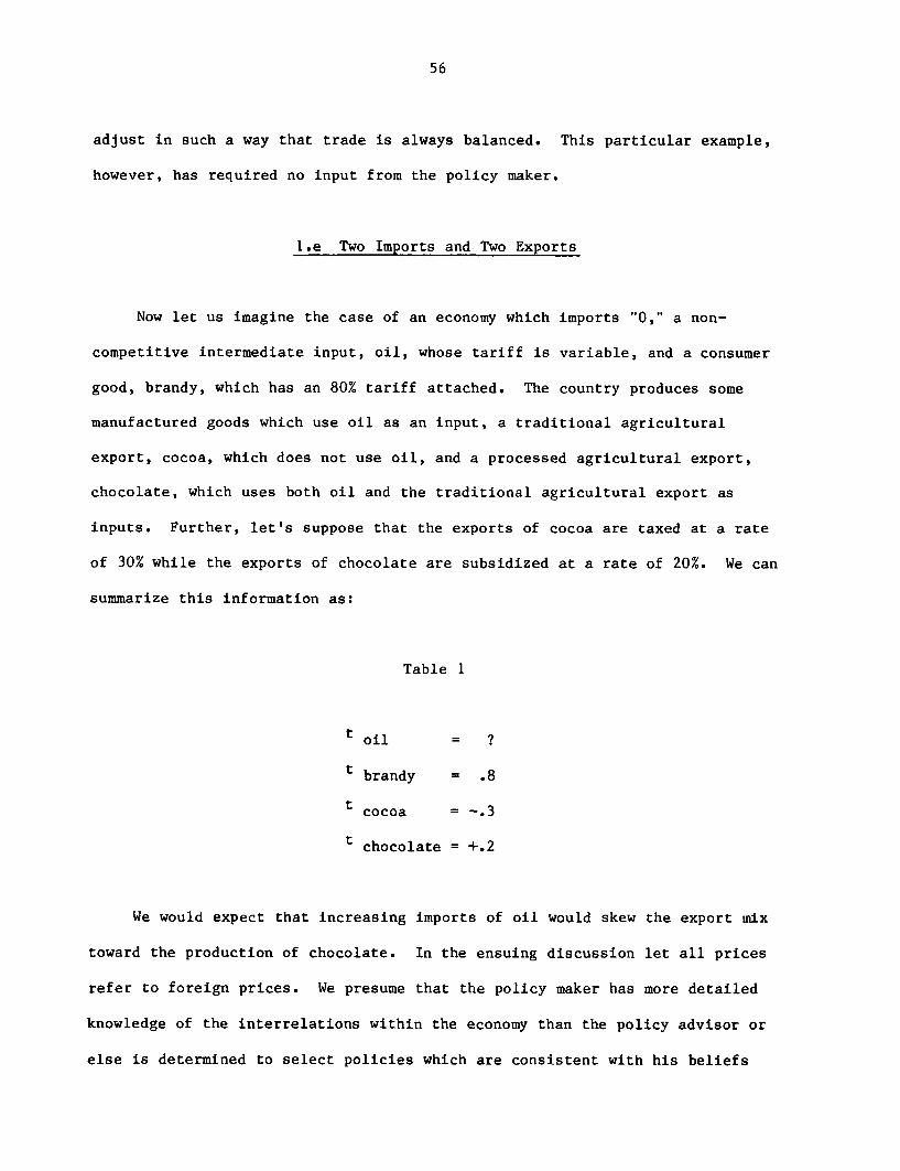
56
adjust in such a way that trade is always balanced. This particular example,
however, has required no input from the policy maker.
i.e Two Imports and Two Exports
Now let us imagine the case of an economy which imports '0," a non-
competitive intermediate input, oil, whose tariff is variable, and a consumer
good, brandy, which has an 80% tariff attached. The country produces some
manufactured goods which use oil as an input, a traditional agricultural
export, cocoa, which does not use oil, and a processed agricultural export,
chocolate, which uses both oil and the traditional agricultural export as
inputs. Further, let's suppose that the exports of cocoa are taxed at a rate
of 30% while the exports of chocolate are subsidized at a rate of 20%. We can
summarize this information as:
Table 1
t oil = ?
t brandy = .8
t cocoa = -.3
t chocolate = +.2
We would expect that increasing imports of oil would skew the export mix
toward the production of chocolate. In the ensuing discussion let all prices
refer to foreign prices. We presume that the policy maker has more detailed
knowledge of the interrelations within the economy than the policy advisor or
else is determined to select policies which are consistent with his beliefs
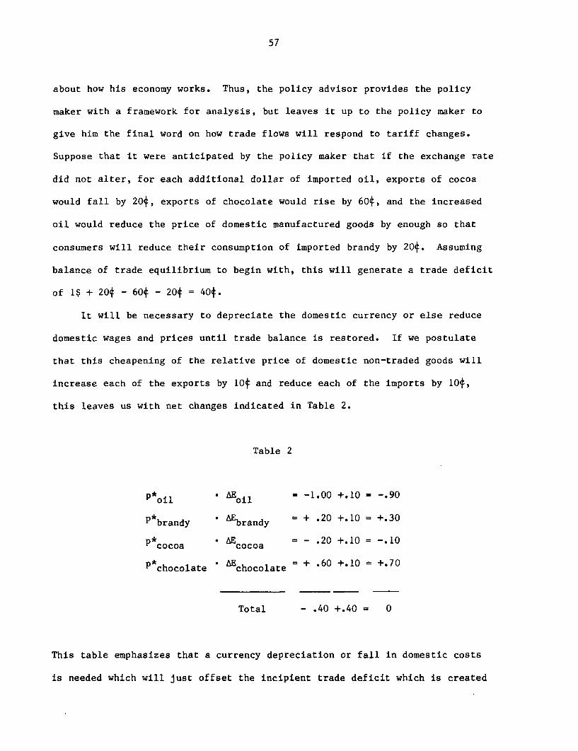
57
about how his economy works. Thus, the policy advisor provides the policy
maker with a framework for analysis, but leaves it up to the policy maker to
give him the final word on how trade flows will respond to tariff changes.
Suppose that it were anticipated by the policy maker that if the exchange rate
did not alter, for each additional dollar of imported oil, exports of cocoa
would fall by 20¢, exports of chocolate would rise by 60¢, and the increased
oil would reduce the price of domestic manufactured goods by enough so that
consumers will reduce their consumption of imported brandy by 20¢. Assuming
balance of trade equilibrium to begin with, this will generate a trade deficit
of 1$ + 20¢ - 60¢ - 20¢ = 40¢.
It will be necessary to depreciate the domestic currency or else reduce
domestic wages and prices until trade balance is restored. If we postulate
that this cheapening of the relative price of domestic non-traded goods will
increase each of the exports by 10¢ and reduce each of the imports by 10¢,
this leaves us with net changes indicated in Table 2.
Table 2
P* oil a&AE oil = -1.00 +.10 = -.90
P* brandy AEbrandy = + .20 +.10 = +.30
P* cocoa 0 AEcocoa =- .20 +.10 = -. 10
P* chocolate Echocolate + *60 +.10 +.70
Total - .40 +.40 = 0
This table emphasizes that a currency depreciation or fall in domestic costs
is needed which will just offset the incipient trade deficit which is created
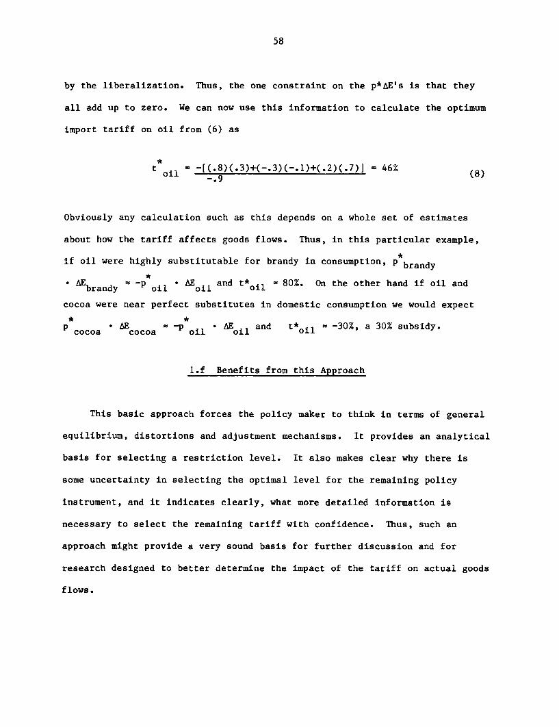
58
by the liberalization. Thus, the one constraint on the p*AE's is that they
all add up to zero. We can now use this information to calculate the optimum
import tariff on oil from (6) as
t oil = -[(.8)(.3)+(-.3)(-.1)+(.2)(.7)] = 46% (8)-.9
Obviously any calculation such as this depends on a whole set of estimates
about how the tariff affects goods flows. Thus, in this particular example,
if oil were highly substitutable for brandy in consumption, P brandy.AE -n .~~ andt* ~ . On the ~n P bra1dy
brandy N oil and t* 80%. On the other hand if oil and
cocoa were near perfect substitutes in domestic consumption we would expect
P*coa cocoa o lp * El and t*oil X -30%, a 30% subsidy.
1.f Benefits from this Approach
This basic approach forces the policy maker to think in terms of general
equilibrium, distortions and adjustment mechanisms. It provides an analytical
basis for selecting a restriction level. It also makes clear why there is
some uncertainty in selecting the optimal level for the remaining policy
instrument, and it indicates clearly, what more detailed information is
necessary to select the remaining tariff with confidence. Thus, such an
approach might provide a very sound basis for further discussion and for
research designed to better determine the impact of the tariff on actual goods
flows.
59
1.g Possible Extentions
Once the basic approach presented here is agreed upon as being a sensible
way to approach the problem, it is easy conceptually to add other distortions
like monopoly power, excise taxes, minimum wages, variable world prices,
externalities both in consumption and production, and distribution weights in
final consumption, or differential utilities attached to consumption and
investment.
Moreover, one can build a general equilibrium model and linearize it
along the lines of Chapter II to calculate more precisely the changes in goods
flows in response to changing tariffs. Such a job can be done with the com-
puter for disaggregated models or else by hand for highly aggregated models.
Moreover, if one takes the view that the truly optimum tariff structure should
seek to minimize rent seeking,2 should be perceived as "fair" by the man in
the street, and should be easy and low cost to administer, then one may want
to have only a few different tariff categories. In such a case, it would be
possible to work with fairly simple highly aggregated sorts of models, so the
analysis itself need not be costly.
20n rent seeking, see the essays by Diamond, Bhagwati, Krugman, Findlay andWellisz, Feenstra and Bhagwati, and Baldwin in Bhagwati (1982) and thereferences therein.
60
III.2 ON USING A SINGLE TARIFF TO EXPLOIT MARKET
POWER ON MANY TRADED GOODS*
2.a Introduction
In this essay, we explore a second application of our basic model.
Namely, we show how to determine the optimum level of the only tariff which we
permit to be variable given the presence of other fixed tariffs and externali-
ties, in this case variable world prices which reflect a country's monopsony
or monopoly power on world markets. Thus world price deviates from the
country's marginal revenue or marginal expenditure and it is desirable from
the individual country's standpoint to use tariffs to correct this distortion.
We obtain the important result that the distortion associated with trade in
any commodity is simply the excess of the tariff over the optimum one, where
the optimum tariff is evaluated using parameters at the observed equilibrium.
We then apply this result to a recent paper by Yabuuchi (1982) on the rela-
tionship between tariff-induced capital inflows and immizeration where foreign
profits are subject to taxation. In the concluding section we show that our
result also applies when foreign markets are interrelated.
2.b Non-Interrelated Foreign Commodity Markets
Consider an economy with distortionless internal markets. We define the
exchange rate between domestic and foreign currency to be unity and normalize
the marginal utility of expenditure of one unit of domestic currency as unity.
*This essay was co-authored with Harold 0. Fried. The authors are grateful toS. Yabuuchi for helpful comments.
61
Then the change in domestic utility can be written just as in the previous
section, as
dy = p dMI (1)
where Pi is the domestic price of the i'th good and Mi is the country's net
imports of the i'th good, i.e. foreign net exports of the ith good.
The balance of payments relationship is
E p*M. = F (2)i Iii
where p* is the foreign price of the i'th good and F is the rate at which
foreign exchange reserves are drawn down.
Define the elasticity of foreign excess supply as
0i = (&MI/dp*i)/(M /p*t) (3)
where dMi/dp* > 0, Mi > 0 for imports and Mi < 0 for exports, so a* > 0 for
imports and o* < 0 for exports.i
Let ti be the import tariff or export subsidy (border tax for short) on
the i'th good expressed as a fraction of the foreign price, so that domestic
and foreign prices are related by
P (1 + ti)P*. (4)
Thus a negative ti denotes an import subsidy or export tariff.
Differentiating (2), and substituting (3) into the result yields
62
E [I + (1/a*)]p*dM = F (5)
which states that the marginal expenditure on good i (the extra foreign
exchange spent to acquire one more unit of i) is [1 + (1/ai)]p*, where F is
defined as the autonomous increase in the rate at which foreign exchange is
used up.
Substituting (4) into (1) and subtracting (5) from the result yields
dy - F = E [t - (1/a*)]p*dM . (6)ii i ii
This means that marginal utility exceeds marginal expenditure on i by
[ti - (1/o*)]p. Thus the border tax which equates the two, i.e. the optimum
border tax, is t* = I/a*. 1i i
Equation (6) can be rewritten as
dy = E [t - t*]p*dM + F = E 6 p*dM + F (7)
where 6 is defined as ti - t*, the excess of the border tax on the i'th good
above its optimum level, where its optimum level is defined with reference to
the elasticity at the prevailing (not necessarily optimum) equilibrium. Thus,
6i is the net benefit from the domestic economy's standpoint associated with a
unit increase in net imports of the i'th good. The lesson of (7) is that any
policy which increases net imports of any good with a positive excess border
'This is the first best optimum tax in the sense that if all sectors are taxedaccordingly, welfare is maximized. The Lerner symmetry theorem implies thatwe can choose one optimum tariff arbitrarily, and through our procedure ofnormalizing marginal utility, we have arbitrarily set the optimum tariffapplying to commodities in perfectly elastic excess foreign supply equal tozero.
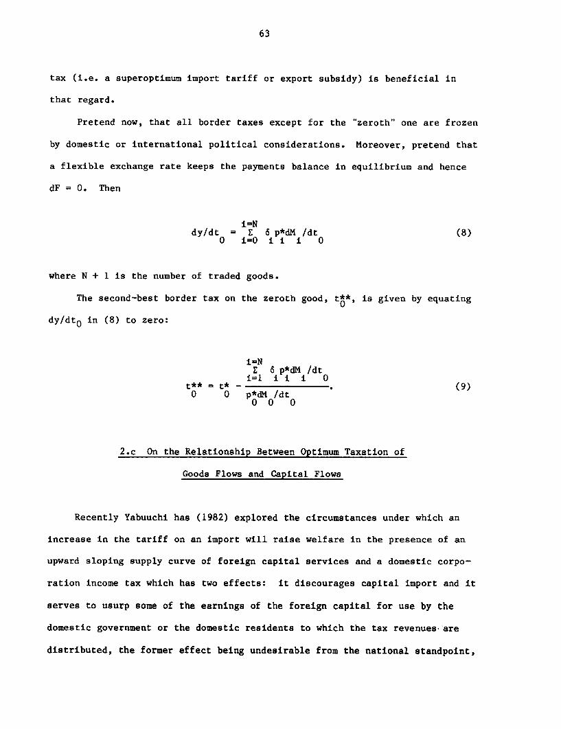
63
tax (i.e. a superoptimum import tariff or export subsidy) is beneficial in
that regard.
Pretend now, that all border taxes except for the "zeroth" one are frozen
by domestic or international political considerations. Moreover, pretend that
a flexible exchange rate keeps the payments balance in equilibrium and hence
dF = 0. Then
i=Ndy/dt 6 p*dM /dt (8)
0 iO i i i 0
where N + 1 is the number of traded goods.
The second-best border tax on the zeroth good, t**, is given by equating
dy/dtO in (8) to zero:
i=NE 6 p*dM /dt
i=1 i i i 0t** = t*- (9)0 0 p*d /dt
00 0
2.c On the Relationship Between Optimum Taxation of
Goods Flows and Capital Flows
Recently Yabuuchi has (1982) explored the circumstances under which an
increase in the tariff on an import will raise welfare in the presence of an
upward sloping supply curve of foreign capital services and a domestic corpo-
ration income tax which has two effects: it discourages capital import and it
serves to usurp some of the earnings of the foreign capital for use by the
domestic government or the domestic residents to which the tax revenues- are
distributed, the former effect being undesirable from the national standpoint,
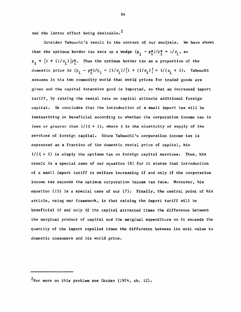
64
and the latter effect being desirable.2
Consider Yabuuchi's result in the context of our analysis. We have shown
that the optimum border tax sets up a wedge (p - P*)/P* = 1/01, soi i i
Pi = [I + (1/ai)]p*. Thus the optimum border tax as a proportion of the
domestic price is (p - P*)/pi = (11 + (I/a,)] = 1I(a, + 1). Yabuuchi
assumes in his two commodity world that world prices for traded goods are
given and the capital intensive good is imported, so that an increased import
tariff, by raising the rental rate on capital attracts additional foreign
capital. He concludes that the introduction of a small import tax will be
immiserizing or beneficial according to whether the corporation income tax is
less or greater than 1/(C + 1), where g is the elasticity of supply of the
services of foreign capital. Since Yabuuchi's corporation income tax is
expressed as a fraction of the domestic rental price of capital, his
1/(E + 1) is simply the optimum tax on foreign capital services. Thus, his
result is a special case of our equation (8) for it states that introduction
of a small import tariff is welfare increasing if and only if the corporation
income tax exceeds the optimum corporation income tax rate. Moreover, his
equation (15) is a special case of our (7). Finally, the central point of his
article, using our framework, is that raising the import tariff will be
beneficial if and only if the capital attracted times the difference between
the marginal product of capital and the marginal expenditure on it exceeds the
quantity of the import repelled times the difference between its unit value to
domestic consumers and its world price.
2For more on this problem see Corden (1974, ch. 12).
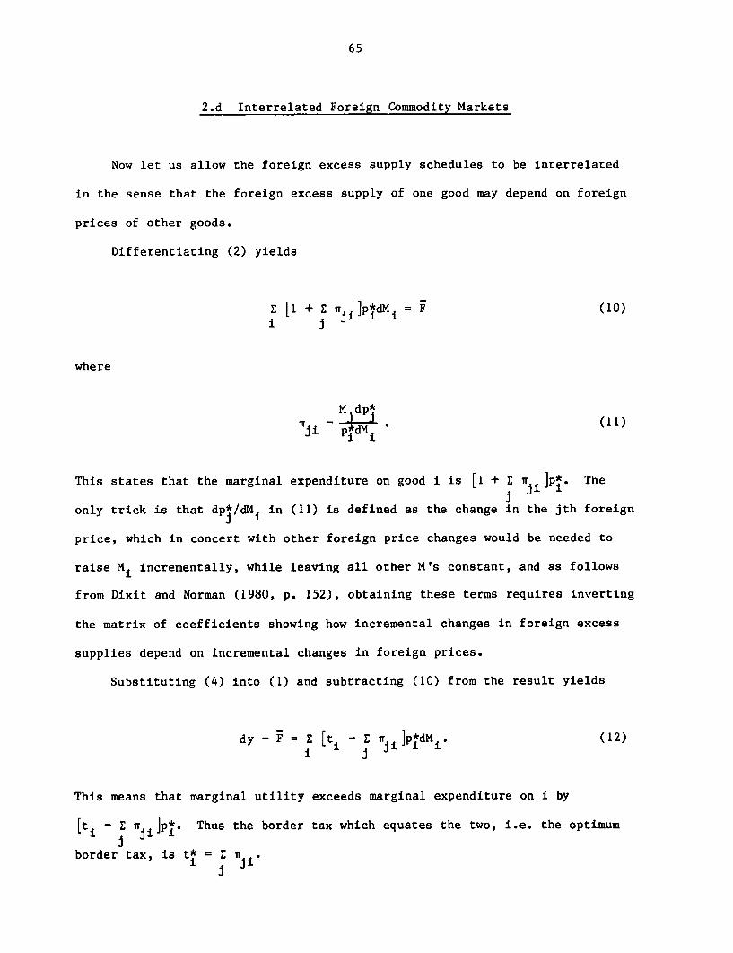
65
2.d Interrelated Foreign Commodity Markets
Now let us allow the foreign excess supply schedules to be interrelated
in the sense that the foreign excess supply of one good may depend on foreign
prices of other goods.
Differentiating (2) yields
E [I + E w i]p*dMi = F (10)i Ji
where
M dp*
Mi *
This states that the marginal expenditure on good i is [I + : w]p* The
only trick is that dp/dMi in (11) is defined as the change in the jth foreign
price, which in concert with other foreign price changes would be needed to
raise Mi incrementally, while leaving all other M's constant, and as follows
from Dixit and Norman (1980, p. 152), obtaining these terms requires inverting
the matrix of coefficients showing how incremental changes in foreign excess
supplies depend on incremental changes in foreign prices.
Substituting (4) into (1) and subtracting (10) from the result yields
dy - F = E [t1 E Tr ]pdMi (12)
This means that marginal utility exceeds marginal expenditure on i by
[ti - E T ipi Thus the border tax which equates the two, i.e. the optimumb j i i
border tax, is t* =E iri ii

66
With this generalized definition of t*, equations (7), (8) and (9) follow.
Thus, the existence of interrelated foreign commodity markets changes
none of the logic of the second section, except it forces us to generalize our
definition of marginal expenditure and consequently the expression we use for
the optimum border tax.
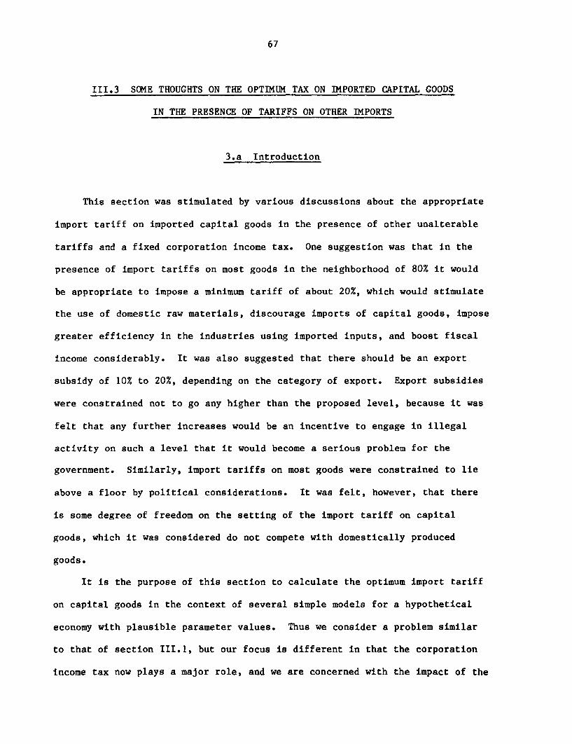
67
III.3 SOME THOUGHTS ON THE OPTIMUM TAX ON IMPORTED CAPITAL GOODS
IN THE PRESENCE OF TARIFFS ON OTHER DMPORTS
3.a Introduction
This section was stimulated by various discussions about the appropriate
import tariff on imported capital goods in the presence of other unalterable
tariffs and a fixed corporation income tax. One suggestion was that in the
presence of import tariffs on most goods in the neighborhood of 80% it would
be appropriate to impose a minimum tariff of about 20%, which would stimulate
the use of domestic raw materials, discourage imports of capital goods, impose
greater efficiency in the industries using imported inputs, and boost fiscal
income considerably. It was also suggested that there should be an export
subsidy of 10% to 20%, depending on the category of export. Export subsidies
were constrained not to go any higher than the proposed level, because it was
felt that any further increases would be an incentive to engage in illegal
activity on such a level that it would become a serious problem for the
government. Similarly, import tariffs on most goods were constrained to lie
above a floor by political considerations. It was felt, however, that there
is some degree of freedom on the setting of the import tariff on capital
goods, which it was considered do not compete with domestically produced
goods.
It is the purpose of this section to calculate the optimum import tariff
on capital goods in the context of several simple models for a hypothetical
economy with plausible parameter values. Thus we consider a problem similar
to that of section III.1, but our focus is different in that the corporation
income tax now plays a major role, and we are concerned with the impact of the
68
tax and tariff structure on the supply of domestic savings. We find that in
certain circumstances this optimum tariff might even be zero or negative.
3.b One Good Is Consumed Domestically; No Corporation Income Tax
First, consider a simple model where only one good is produced in a
country using imported capital goods and domestic labor. In that case, in the
free-trade equilibrium we would import capital goods in order to produce some
of our output, part of which would be sold abroad to pay for our imports of
physical capital goods. Thus, there would be no imports of non-capital items,
so that even if those goods came to be covered by an import tariff, the tariff
would be non-binding. If on the other hand, we subsidized the exports of the
single good, first best policy would require that we impose a tax on the
import of the capital good at precisely the same rate. According to this
argument, our country should tax imported capital goods at 10 to 20% to match
the export subsidy.1
3.c A Model With One Imported Consumption Good and One Domestically Produced
Good Which is Both Consumed Domestically and Exported, Where all Capital is
Imported, and A Corporation Income Tax Distorts Savings Decisions
In order to analyze this problem it is necessary to build a formal model.
Let dy = pcdC + pmdM + r[l-uI[pcdCo + pMdMo] (1)
where
lWe assume that both the export subsidy and the import tariff are based on theforeign prices of the goods in question.
69
y is the domestic utility defined so that one unit of domestic currency is
worth one util,
PC is the domestic currency price of the domestic good,
Pm is the domestic currency price of the imported consumer good,
r is the before tax real rate of return on capital, and
u is the corporation tax rate. Thus r[l-u] is the after tax real rate of
interest.
C and M are respectively, steady state consumption of the domestic good and
the imported consumer good.
C0 and Mo are respectively, consumption of the domestic good and the imported
consumer good in period zero.
E and E are respectively exports of the domestic good generally and in period
0.
Equation (1) can be understood as follows. The first two terms represent
the increment in utility from increased steady state consumption of the two
goods. The consumption of the two goods is weighted by the corresponding
price, because individuals equate price to marginal utility when the marginal
utility of money is one, as we have defined it here. Individuals save until
the after-tax real rate of return comes to equal their rate of time prefer-
ence. Thus, the after-tax real rate of interest is simply the marginal
utility of a one period increase in consumption relative to the marginal
utility of the same steady state increase in consumption. Since we permit
only differential changes in prices over our infinite time horizon, the
coefficients for one period consumption changes are the same as those for
steady-state changes, except they are multiplied by the real rate of interest.
We define a unit of each good, so that its world price is unity, and
domestic prices are equal to foreign prices adjusted by the import tariff or
70
export subsidy. Thus, we have
PC (l+8)p = 1 + (2)
Pm = (1+tm)Pm = I + tm (3)
Pk (l+tk)pk =I + tk (4)
where
Pk is the domestic price of the capital good,
* * *
Pcs Pm' Pk are foreign prices
s is the subsidy on the export of the domestic good expressed as a fraction of
its foreign price, and
tm and tk are the import tariffs on the imported consumption good and capital
good respectively.
We have defined one unit of each good as that quantity which sells for
one unit of foreign currency on the world market. Hence each foreign price is
set equal to one. Moreover foreign prices are assumed to be fixed.
Also, we define a unit of domestic currency as that quantity which
exchanges for one unit of foreign currency, so that the exchange rate does not
explicitly enter equations (2), (3) or (4).
International trade can be used to transform consumption goods into
capital goods according to
dK - M+ dE (5)
where
dK is the change in the economy's stock of the capital good.
71
This means that by giving up consumption of one unit of either consump-
tion good and exporting it or ceasing to import it in exchange for one more
unit of the capital good, the economy can increase its capital stock by one
unit. Incidentally, throughout this analysis we assume that no capital is
produced at home, so that it must all be imported.
Let 6 be the rate at which the capital stock depreciates. Then we can
write steady-state imports of capital as 6 K. Thus, our steady-state balance-
of-trade equation becomes
dM + 6dK = dE (6)
where
M is imports of the imported consumption good and E is exports of the
domestically produced good.
Since domestic production of the domestically produced good, D, must equal
what is consumed plus what is exported:
D = C + E. (7)
Since capital is paid its marginal product plus depreciation
pc dD- d = r + (8)p dK
where
Pk is the domestic currency price of capital
and
dD aD is the marginal product of capital.
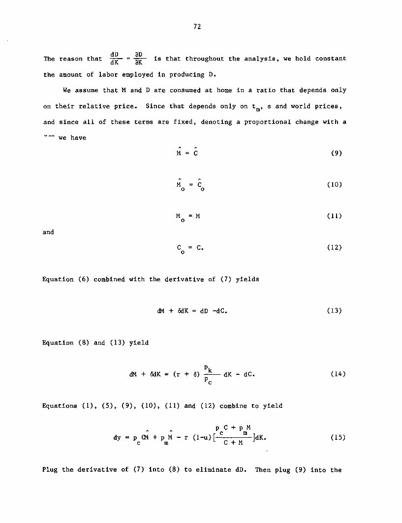
72
The reason that dD 'D is that throughout the analysis, we hold constant
the amount of labor employed in producing D.
We assume that M and D are consumed at home in a ratio that depends only
on their relative price. Since that depends only on tm$ s and world prices,
and since all of these terms are fixed, denoting a proportional change with a
we have
M= C (9)
M = C (10)o o
M = M (11)0
and
C = C. (12)0
Equation (6) combined with the derivative of (7) yields
dM + &dK = dD -dC. (13)
Equation (8) and (13) yield
dM + 6dK = (r + 6) p dK - dC. (14)
Equations (1), (5), (9), (10), (11) and (12) combine to yield
p C + p M
dy - p CM + p M - r (1-u)[ C + M ]dK-(15)C m d M (td9
Plug the derivative of (7) into (8) to eliminate dD. Then plug (9) into the
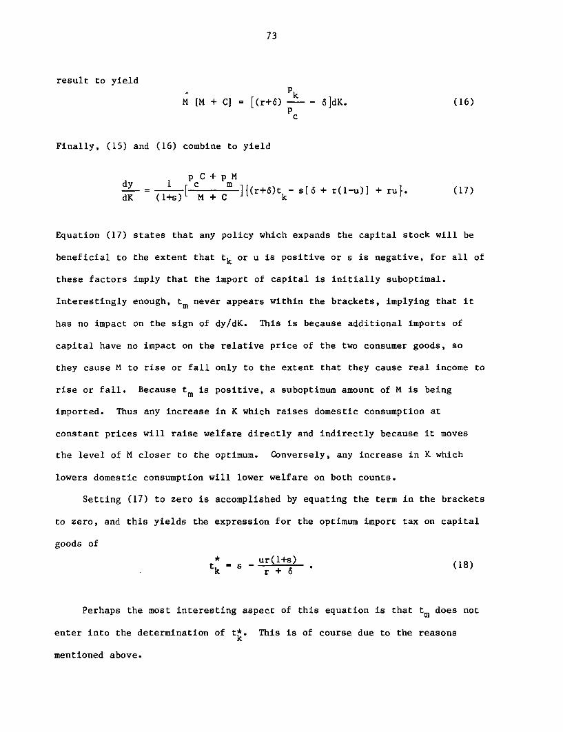
73
result to yield
M [M + C] = [(r+6) - - 6]dK. (16)
c
Finally, (15) and (16) combine to yield
p C + pM
dy = 1I+ c[ M m+ C ]{(r+6)t - s[5 + r(1-u)I + ru (17)dK (1+s) M +C k r 1
Equation (17) states that any policy which expands the capital stock will be
beneficial to the extent that tk or u is positive or s is negative, for all of
these factors imply that the import of capital is initially suboptimal.
Interestingly enough, tm never appears within the brackets, implying that it
has no impact on the sign of dy/dK. This is because additional imports of
capital have no impact on the relative price of the two consumer goods, so
they cause M to rise or fall only to the extent that they cause real income to
rise or fall. Because tm is positive, a suboptimum amount of M is being
imported. Thus any increase in K which raises domestic consumption at
constant prices will raise welfare directly and indirectly because it moves
the level of M closer to the optimum. Conversely, any increase in K which
lowers domestic consumption will lower welfare on both counts.
Setting (17) to zero is accomplished by equating the term in the brackets
to zero, and this yields the expression for the optimum import tax on capital
goods of
ur(l+s) (18)
Perhaps the most interesting aspect of this equation is that tm does not
enter into the determination of tk. This is of course due to the reasonsk
mentioned above.
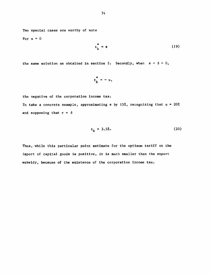
74
Two special cases are worthy of note
For u = 0
*tk = 5 (19)
the same solution as obtained in section 2. Secondly, when s = 6 = 0,
tk =-u,
the negative of the corporation income tax.
To take a concrete example, approximating s by 15%, recognizing that u = 20%
and supposing that r 6
tk = 3.5%. (20)
Thus, while this particular point estimate for the optimum tariff on the
import of capital goods is positive, it is much smaller than the export
subsidy, because of the existence of the corporation income tax.
75
III.4 OPTIMUM TAXES ON IMPORTED CAPITAL GOODS AND
INTERMEDIATE GOODS
4.a Introduction
This section pursues further the calculation of optimum tariffs on
imported capital goods and intermediate products for a hypothetical less
developed country, given that certain other tariffs and export subsidies are
fixed. An initial attempt at this problem is presented in the previous sec-
tion. In that model, I pretended that only one good was produced domesti-
cally, using domestic labor and imported capital. This paper by contrast
assumes a model which is laid out schematically in Figure 1, and uses it to
determine the optimum import tariffs on imported capital and intermediate
inputs, given that all other taxes and subsidies on international trade are
fixed.
As indicated in the conclusion, the model is constructed in order to
indicate some of the contributions to policy analysis that linear models can
make. In essence, my goal in this and other sections is to illustrate simple
tractable methodologies for applying cost-benefit analysis to small
adjustments in existing tariff and tax structures and the devising of optimal
structures. Or to describe the analysis in yet another way, the problem
attempted in this and other sections is to generalize the logic of Harry G.
Johnson's (1971, Ch. 8) work on the Scientific Tariff from his model in which
traded goods have no input-output structure and the cross-price elasticities
76
of demand between them are implicitly assumed to be zero.1 The approach
suggested here is not hampered by any degree of interdependence between
markets, although in that it is linear, it suffers from the same flaw as
Johnson's does, namely being an approximation.
4.b The Model
In Figure 2, the economy is shown to produce two goods, cocoa which
currently has no export tax or subsidy and chocolate which is subject to a 20%
export subsidy (where throughout the paper all tariffs and subsidies are
expressed as fractions of the world price). Cocoa is produced using land and
labor, and domestic production is either exported or used in the production of
chocolate.
Chocolate is produced with constant returns to scale using two composite
factors, with no substitution between them. The first composite factor is an
aggregate of capital and labor, while the second is an aggregate of cocoa and
flavorings. Both composite factors are first degree homogeneous functions of
the factors which compose them. Both capital and flavorings are imported,
with no duty attached and no domestic production of either. The chocolate
10f course earlier on in that essay Johnson did show how to measure thewelfare impact of tariff changes when cross price demand elasticities aretaken into account. Moreover, he provided a welfare analysis of the effectsof tariffs in a particular input-output context in Johnson (1971, Ch. 13),which could have been applied to the scientific tariff problem. In both ofthese papers, Johnson makes the implicit assumptions that value added in eachsector is produced with a fixed factor (call it capital) which may be combinedin variable proportions with a mobile factor (call it labor), and that as thetariff varies, there is no change in the price of the mobile factor (holdingthe exchange rate constant). However, this requires the twin implicit heroicassumptions that there is at least one tradeable good which is in perfectlyelastic domestic supply and that the effective protection of this good iszero.
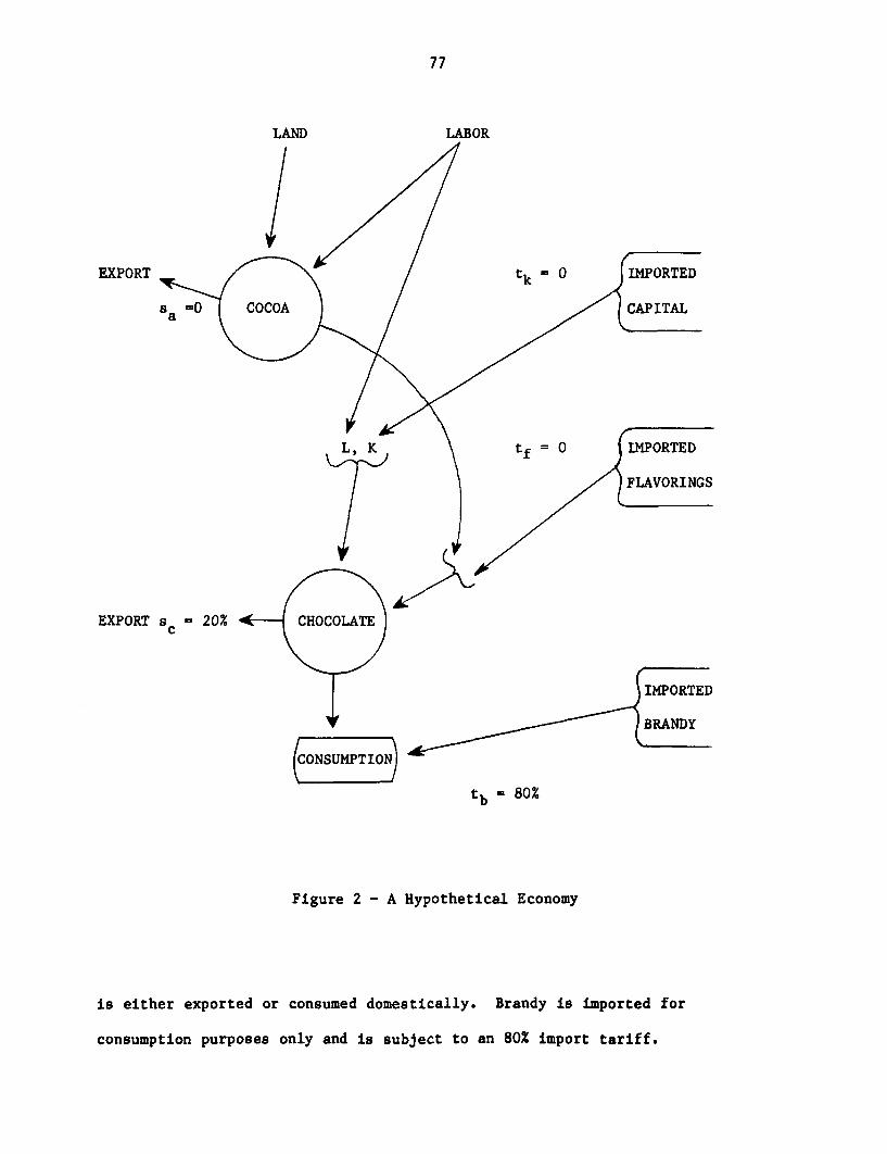
77
LAND LABOR
EXPORT tk m °
L\ K tf = 0 IMPORTED
l < ~~~~~~FLAVORINGS
EXPORT s= 20% CHOCOLATE
CONSUMPTION
tb - 80%
Figure 2 - A Hypothetical Economy
is either exported or consumed domestically. Brandy is imported for
consumption purposes only and is subject to an 80% import tariff.
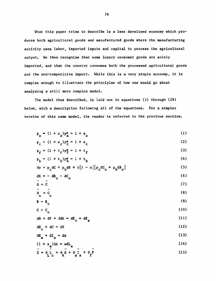
78
What this paper tries to describe is a less developed economy which pro-
duces both agricultural goods and manufactured goods where the manufacturing
activity uses labor, imported inputs and capital to process the agricultural
output. We then recognize that some luxury consumer goods are solely
imported, and that the country consumes both the processed agricultural goods
and the non-competitive import. While this is a very simple economy, it is
complex enough to illustrate the principles of how one would go about
analyzing a still more complex model.
The model thus described, is laid out in equations (1) through (28)
below, with a description following all of the equations. For a simpler
version of this same model, the reader is referred to the previous section.
pa (1 + s)p* = 1 + 8 (1)
PC (+ c)P* 1 + S (2)
Pf = (1+ tf)pf - 1 + tf (3)
= (1+ tb)pb =1 + tb (4)
dy = pcdC + PbdB + r[1 - u][pcdCo + PbdBo] (5)
dK = -dB -dC (6)
B =C (7)
B C (8)o 0
B =B (9)0
C =C (10)
dB + dF + 6dK - dE + dE (11)c a
dE + dC dX (12)c
dE + dI - dA (13)a a
(1 + s a)dA - wdLa (14)A A A A e
X - OL +eoK +B3I + OF (-15)L c k a a f
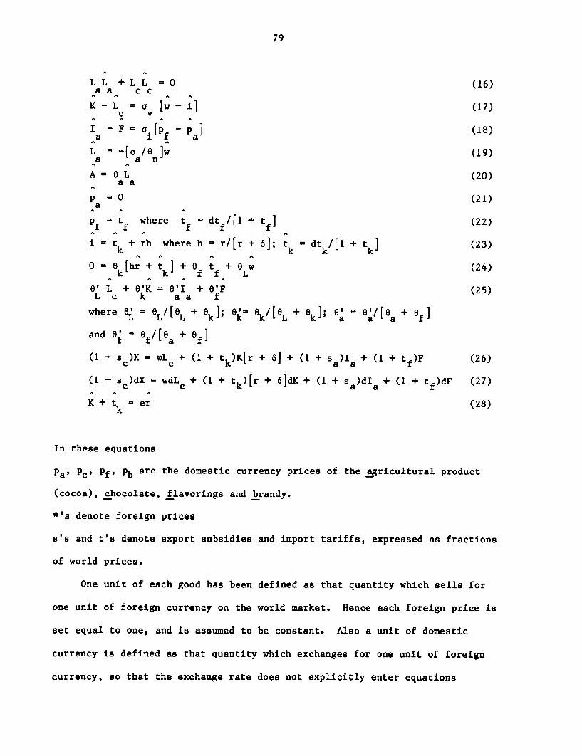
79
LL + LL = 0 (16)
K -L a [w-i] (17)c v
Ia i[ f p a] (18)
L = -[a /6 ]w (19)a a n
A= OaL (20)a a
P =0 (21)a
pf tf where tf = dtf/[1 + t f] (22)
i = tk + rh where h r/[r + 6]; tk dt k/[I + t k] (23)
0=6 k[hr +t k] + wf tf L (24)
0' L + V'K = 0'I + 0'F (25)L c k a a f
where = =L/[L + k]; =k Ok/[OL + k]; a' = ea'/[a + ef]
and 6 Of/['a + Of]
(1 + sc)X = wLc + + tk)K[r + 6] + (I + sa)Ia + (1 + tf)F (26)
(1 + sc)dX = wdLc + (1 + tk)[r + 6]dK + (1 + s a)dIa + (1 + tf)dF (27)
K + t = er (28)
k
In these equations
Pa' PCt Pf, Pb are the domestic currency prices of the gricultural product
(cocoa), chocolate, flavorings and brandy.
*'s denote foreign prices
s's and t's denote export subsidies and import tariffs, expressed as fractions
of world prices.
One unit of each good has been defined as that quantity which sells for
one unit of foreign currency on the world market. Hence each foreign price is
set equal to one, and is assumed to be constant. Also a unit of domestic
currency is defined as that quantity which exchanges for one unit of foreign
currency, so that the exchange rate does not explicitly enter equations
80
(1) - (4). Finally, the exchange rate is held constant and the adjustment
process is assumed to occur through flexible wages and prices.
y is domestic utility defined so that one unit of domestic currency is worth
one util.
r is the before tax real rate of return on capital.
u is the corporation tax rate. Thus r[I - ul is the after tax real rate of
interest.
C and B are respectively, steady state consumption of chocolate and brandy.
CO and Bo are respectively, consumption of chocolate and brandy in period
zero. Since all brandy is imported, Bo and B represent imports of brandy in
the initial period and in steady state equilibrium respectively.
Equation (5) can be understood as follows. The first two terms represent
the increment in utility from increased steady state consumption of the two
goods. The consumption of the two goods is weighted by the corresponding
price, because individuals equate price to marginal utility when the marginal
utility of money is one, as we have defined it here. Individuals save until
the after-tax real rate of return comes to equal their rate of time
preference. Thus, the after-tax real rate of interest is simply the marginal
utility of a one period increase in consumption relative to the marginal
utility of the same steady state increase in consumption. Since we permit
only differential changes in prices over our infinite time horizon, the prices
attached to one period consumption changes are the same as those for steady-
state changes, except they are multiplied by the real rate of interest.
International trade can be used to transform consumption goods into
capital goods according to (6) where
dK is the change in the economy's stock of the capital good.
This means that by giving up consumption of one unit of either consump-
81
tion good and exporting it or ceasing to import it in exchange for one more
unit of the capital good, the economy can increase its capital stock by one
unit. Incidentally, throughout this analysis we assume that no capital is
produced at home, so that it must all be imported.
We assume that B and C are consumed at home in a ratio that depends only
on their relative price. Since that depends only on tb, Sc and world prices,
and since all of these terms are fixed, denoting a proportional change with a
. we have (7) and (8); since prices change only infinitesimally, we have (9)
and (10).
Equation (11) is our steady-state balance-of-trade equilibrium condition
where 6 is the rate of depreciation of the capital stock and E c and Ea are
exports of chocolate and cocoa in equilibrium.
Equations (12) and (13) are market clearing conditions for chocolate and
cocoa respectively, where
A is cocoa output,
X is chocolate output and
Ia is the input of cocoa into chocolate manufacture.
Equation (14) states that labor is paid its marginal product in cocoa,
where w is the common wage rate in both sectors and La is labor in cocoa.
Equation (15) is the production function for chocolate, where Lc is labor
in chocolate. The O's represent factor shares. Hence \ + Ok + 6a + Of = 1.
This equation follows from first degree homogeneity and the fact that factors
are each paid their marginal products, and is derived in Chapter I.
Equation (16) is the market clearing condition for labor.
Equation (17) indicates that the elasticity of substitution between labor
and capital in the labor-capital aggregate is av where i is the user cost of
capital.
82
Equation (18) indicates that the elasticity of substitution in forming
the intermediate input aggregate is ai.
Equation (19) is the demand for agricultural labor. It is derived from
a A
the relations: N = 0, L - N = a [n - w] and 0 = w EL + n 6 , where N is
land in cocoa, La is labor in cocoa, and n is the rental rate on land.
Equation (20) is an alternative version of (14) and states that labor in
cocoa is paid its marginal product. Equations (21) and (22) are the
differential forms of (1) and (3) respectively.
Equation (23) is the differential form of i = r + 6) =
(1 + tk) (r + 6), which defines the user cost of capital.
Equation (24) is the dual of (15) with the recognition of (23) and that
the fixed sa and 5c mean that p = p = 0.
Equation (25) states that the proportional change in the L,K aggregate
must equal the proportional change in the A,F aggregate, and is an implication
of the assumption that the two aggregates are combined in fixed proportions.
Equation (26) is the product exhaustion statement for chocolate and (27)
states that factors are paid their marginal products.
Finally, (28) indicates that the value of capital goods which individuals
are willing to hold depends on the real rate of return, with e > 0 being the
elasticity of demand for wealth held in the form of capital goods.
4.c Distortions, Stocks, Flows and Welfare
Equations (1) - (10) combine to yield
pCp (pB
dy = [pcC + pbB]C - r[1 - u] [I C + B ]dK. (29)
83
Equations (7), (11), and (12) combine to yield
dB + dC = [B + C]C = -dF - 6dK + dX + dE a (30)
Equations (13), (14), (16) and (27) combine to yield
O = -(1 + s c)dx - (I + sa )dEa + (I + tk)(r + 6)dK + (1 + tf)dF. (31)
Equations (30) and (31) combine to yield
[B + C] C = -s dX - s dE + tfdF + tk ddK + (1 + tk )rdK. (32)
Finally, (29) and (32) combine to yield
dy = a{-scdX - sadEa + tfdF + [tk6 + (tk + u)r]dK} (33)
p C + pbBwhere a =
Equation (33) is plausible, because the expression in the brackets is
simply the sum of the changes in the flows or the capital stock multiplied by
the attached distortions, and a is simply the utility value of a unit of
foreign exchange. Regrettably, I have been unable to come up with an
intuitive verification of the precise form taken by (33). However, if r - 0,
the expression inside the braces becomes simply the change in the economy's
net output valued at world prices.
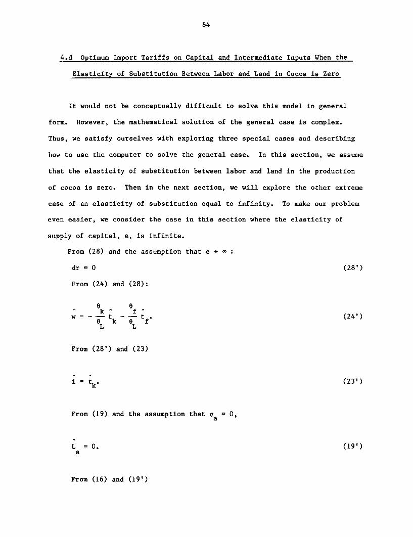
84
4.d Optimum Import Tariffs on Capital and Intermediate Inputs When the
Elasticity of Substitution Between Labor and Land in Cocoa is Zero
It would not be conceptually difficult to solve this model in general
form. However, the mathematical solution of the general case is complex.
Thus, we satisfy ourselves with exploring three special cases and describing
how to use the computer to solve the general case. In this section, we assume
that the elasticity of substitution between labor and land in the production
of cocoa is zero. Then in the next section, we will explore the other extreme
case of an elasticity of substitution equal to infinity. To make our problem
even easier, we consider the case in this section where the elasticity of
supply of capital, e, is infinite.
From (28) and the assumption that e + X
dr = 0 (28')
From (24) and (28):
e 1k f
OL k oL f(2'L L
From (28') and (23)
i = tk. (23')
From (19) and the assumption that a 0,
L = O. (19')a
From (16) and (19')
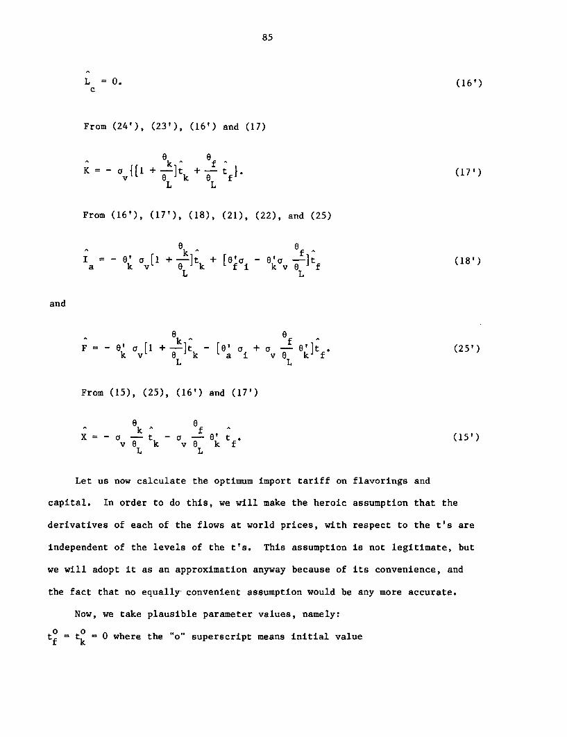
85
L = 0. (16')
From (24'), (23'), (16') and (17)
K=- a {[1 + -it + t I. (17')V 0 k 0 f
L L
From (16'), (17'), (18), (21), (22), and (25)
^ ~~~~k ^ 6 I - eok a [1 + o ]tk + [%ai - Ov aO]tf (18')
L L
and
^ k ^ fF = - 0' a [1 + -]t - [0' a + a - 0'kt . (25')k v 0L k a i vLk
L L
From (15), (25), (16') and (17')
0 0k ~~~f
X=-a tk- -0'l t .(15')
v O k v O k fL L
Let us now calculate the optimum import tariff on flavorings and
capital. In order to do this, we will make the heroic assumption that the
derivatives of each of the flows at world prices, with respect to the t's are
independent of the levels of the t's. This assumption is not legitimate, but
we will adopt it as an approximation anyway because of its convenience, and
the fact that no equally convenient assumption would be any more accurate.
Now, we take plausible parameter values, namely:
to = to = 0 where the "o" superscript means initial valuef k
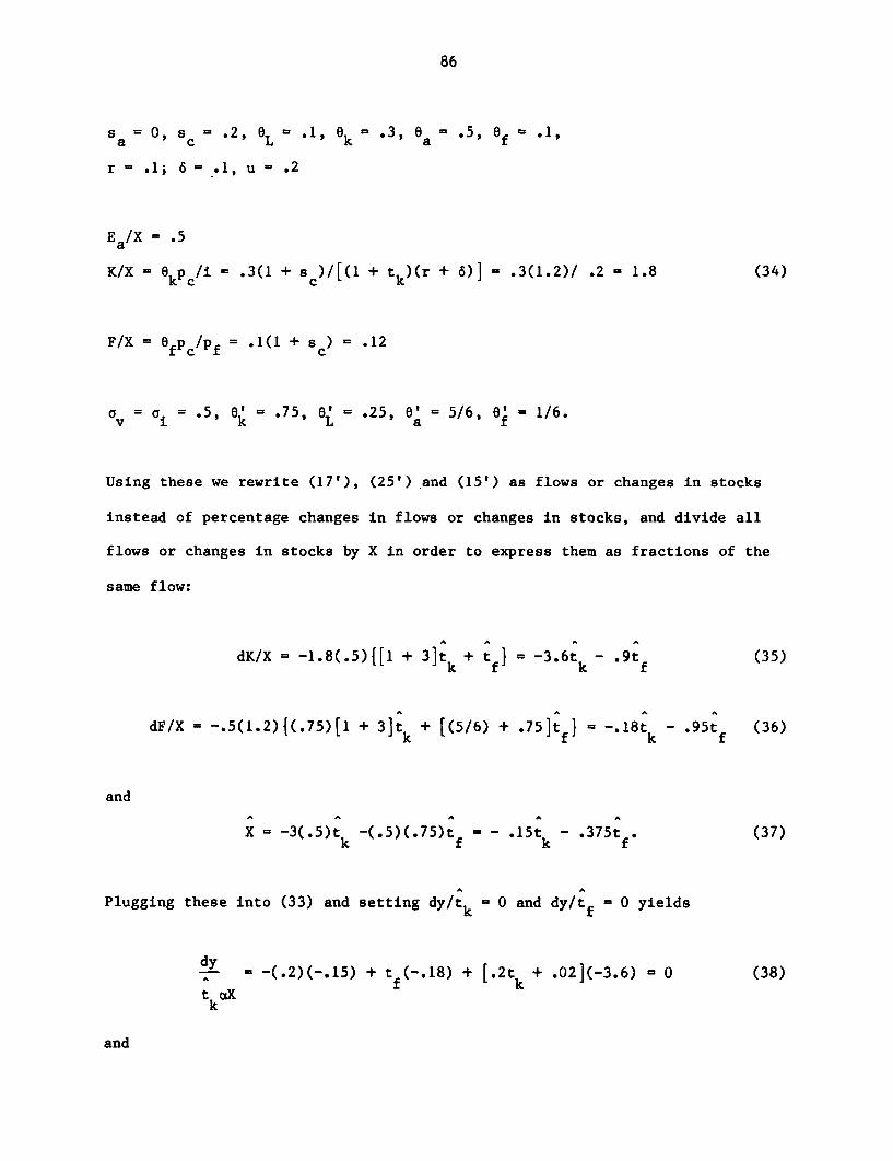
86
S = 0,s S= .2, 3L = .1, k=.3,9 a=5,O
r = .1; 6 = .1, u = .2
Ea/X = .5
K/X 6kpc/i .3(1 + sc)/[(l + tk)(r + 6)] = .3(1.2)/ .2 = 1.8 (34)
FIX ffPc /Pf .1(1 + sc) = .12
av a = .5' = *75' 0' = .25, 0' = 5/6, 0' = 1/6.
Using these we rewrite (17'), (25') and (15') as flows or changes in stocks
instead of percentage changes in flows or changes in stocks, and divide all
flows or changes in stocks by X in order to express them as fractions of the
same flow:
dK/X = -1.8(.5){[1 + 3]t + t } = -3.6t - .9t (35)k f k f
dF/X = -.5(1.2){(.75)[1 + 3]tk + [(5/6) + .75]tfI} -.18tk - *95tf (36)
and
X = -3(.5)tk -(.5)(.75)tf - .15tk - .375t . (37)
Plugging these into (33) and setting dy/tk 0 and dy/tf = 0 yields
dy = -(.2)(-.15) + t f(-.18) + [.2tk + .02](-3.6) = 0 (38)
aka
and
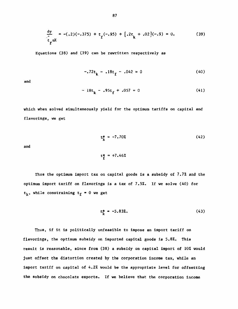
87
dy = -(.2)(-.375) + t (-.95) + [.2t + .02](-.9) = 0. (39)f k
t agxf
Equations (38) and (39) can be rewritten respectively as
-.72t - 18t - .042 = 0 (40)k * f
and
- 18tk - .95tf + .057 =0 (41)
which when solved simultaneously yield for the optimum tariffs on capital and
flavorings, we get
t* = -7.70% (42)
and
t* = +7.46%
Thus the optimum import tax on capital goods is a subsidy of 7.7% and the
optimum import tariff on flavorings is a tax of 7.5%. If we solve (40) for
tk, while constraining tf - 0 we get
tk = -5.83%. (43)k
Thus, if it is politically unfeasible to impose an import tariff on
flavorings, the optimum subsidy on imported capital goods is 5.8%. This
result is reasonable, since from (38) a subsidy on capital import of 10% would
just offset the distortion created by the corporation income tax, while an
import tariff on capital of 4.2% would be the appropriate level for offsetting
the subsidy on chocolate exports. If we believe that the corporation income
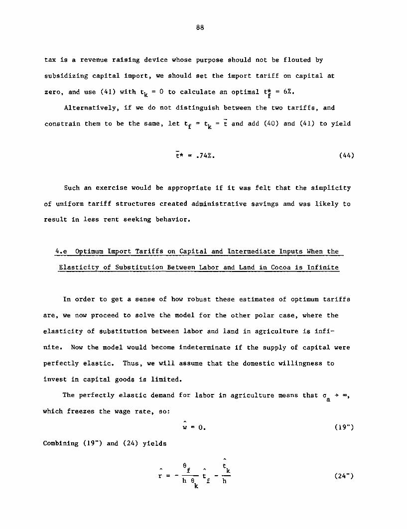
88
tax is a revenue raising device whose purpose should not be flouted by
subsidizing capital import, we should set the import tariff on capital at
zero, and use (41) with tk = 0 to calculate an optimal t* = 6%.k ~~~~~~~~~~~f
Alternatively, if we do not distinguish between the two tariffs, and
constrain them to be the same, let tf = tk = t and add (40) and (41) to yield
t* = .74%. (44)
Such an exercise would be appropriate if it was felt that the simplicity
of uniform tariff structures created administrative savings and was likely to
result in less rent seeking behavior.
4.e Optimum Import Tariffs on Capital and Intermediate Inputs When the
Elasticity of Substitution Between Labor and Land in Cocoa is Infinite
In order to get a sense of how robust these estimates of optimum tariffs
are, we now proceed to solve the model for the other polar case, where the
elasticity of substitution between labor and land in agriculture is infi-
nite. Now the model would become indeterminate if the supply of capital were
perfectly elastic. Thus, we will assume that the domestic willingness to
invest in capital goods is limited.
The perfectly elastic demand for labor in agriculture means that a + ^'
which freezes the wage rate, so:
w 0. (19")
Combining (19') and (24) yields
Of t^ k
r h e f h (24")k
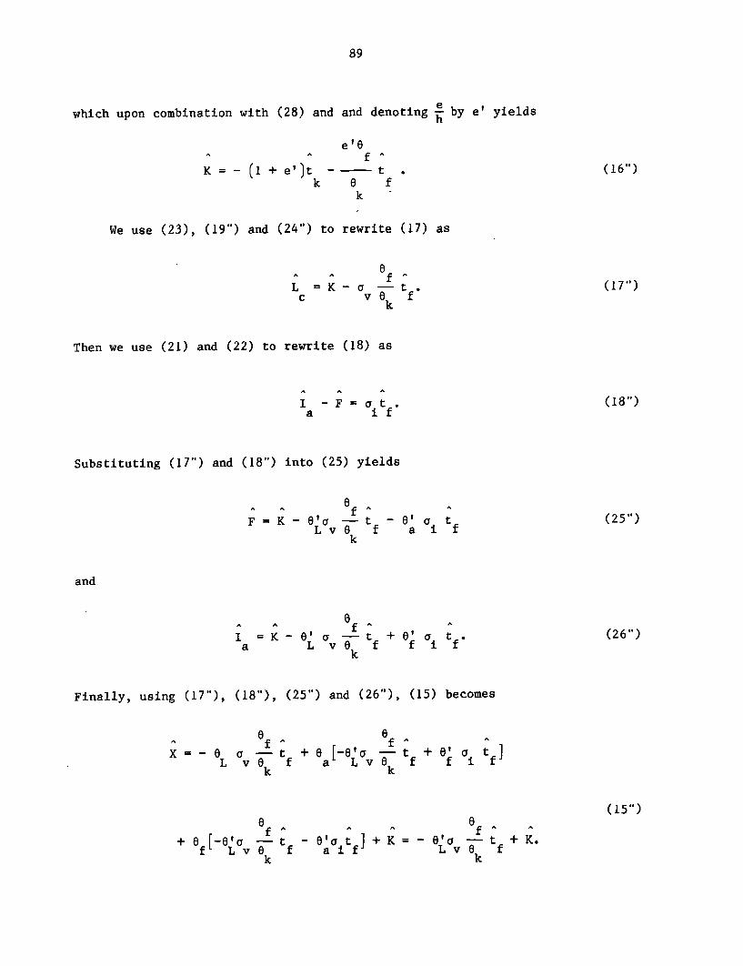
89
which upon combination with (28) and and denoting e by e' yields
e'e-' A f A
K = - (1 + e')t - - t . (16")k u f
k
We use (23), (19") and (24") to rewrite (17) as
A fAL = K - a - t . (17")c v k f
Then we use (21) and (22) to rewrite (18) as
I -F=a t . (18")a i f
Substituting (17") and (18") into (25) yields
8fA F = K - O8a - t -e' a t (25")
Lv f a i fk
and
fI = K - 0' a - t + o' a v (26")a Lv f f i f
k
Finally, using (17"), (18"), (25") and (26"), (15) becomes
A Uf I f I A
X = - 0 a - t + o [-oIa - t + 0 i a, tfL vO k f a L v k f f i f
(15")
+ e [-a'a - t! - 0ait ] + K L'a - tf + K.f Lv f aitf vk k
kk
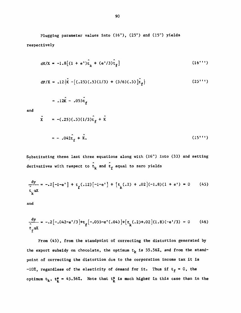
90
Plugging parameter values into (16"), (25") and (15") yields
respectively
dK/X = -1.8[(1 + e')tk + (e'/3)tf] (16'1')
dF/X = .12{K -[(.25)(.5)(1/3) + (5/6)(.5)]tf} (25'"')
= .12K - .055tf
and
x = -(.25)(.5)(1/3)tf + K
=-- .042tf + K. (15''')
Substituting these last three equations along with (16") into (33) and setting
derivatives with respect to tk and tf equal to zero yields
,dY = -.2[-1-e'] + tf(.12)[-1-e'] + [t k(.2) + .02](-1.8)(1 + e') = 0 (45)t aixk
and
dy = -.2[-.042-e'/3]+t [-.055-e'(.04)]+[t (.2)+.02](1.8)(-e'/3) = 0 (46)f k
tfax
From (45), from the standpoint of correcting the distortion generated by
the export subsidy on chocolate, the optimum tk is 55.56%, and from the stand-
point of correcting the distortion due to the corporation income tax it is
-10%, regardless of the elasticity of demand for it. Thus if tf = 0, the
optimum tk, t* = 45.56%. Note that tk is much higher in this case than in the
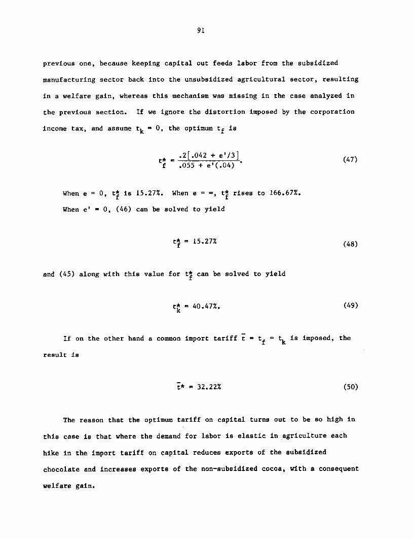
91
previous one, because keeping capital out feeds labor from the subsidized
manufacturing sector back into the unsubsidized agricultural sector, resulting
in a welfare gain, whereas this mechanism was missing in the case analyzed in
the previous section. If we ignore the distortion imposed by the corporation
income tax, and assume tk = 0, the optimum tf is
t* = .2[.042 + e'/3]- ~~~(47)tf ' 055 + e(.04)]47
When e = 0 t* is 15.27%. When e = , t* rises to 166.67%.f ~~~~~~~~f
When e' = 0, (46) can be solved to yield
t* = 15.27% (48)f (8
and (45) along with this value for t* can be solved to yieldf
t* = 40Q47%* (49)
If on the other hand a common import tariff t = tf = tk is imposed, the
result is
t* = 32.22% (50)
The reason that the optimum tariff on capital turns out to be so high in
this case is that where the demand for labor is elastic in agriculture each
hike in the import tariff on capital reduces exports of the subsidized
chocolate and increases exports of the non-subsidized cocoa, with a consequent
welfare gain.
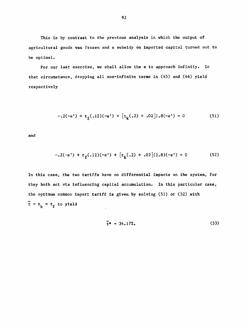
92
This is by contrast to the previous analysis in which the output of
agricultural goods was frozen and a subsidy on imported capital turned out to
be optimal.
For our last exercise, we shall allow the e to approach infinity. In
that circumstance, dropping all non-infinite terms in (45) and (46) yield
respectively
-.2(-e') + tf(.12)(-e') + [tk(.2) + .02]1.8(-e') = 0 (51)
and
-.2(-e') + tf(.12)(-e') + [tk(.2) + .02](1.8)(-e') 0 (52)
In this case, the two tariffs have no differential impacts on the system, for
they both act via influencing capital accumulation. In this particular case,
the optimum common import tariff is given by solving (51) or (52) with
t = tk = tf to yield
t* = 34.17%. (53)
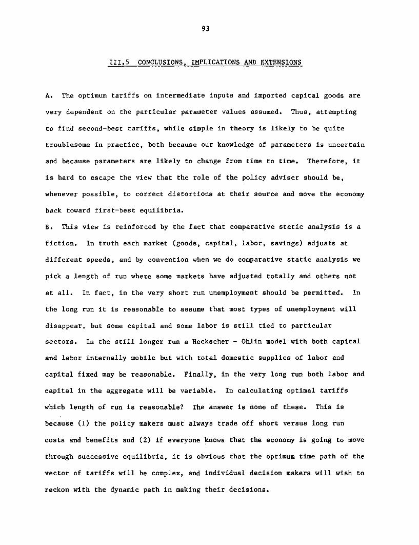
93
III.5 CONCLUSIONS, IMPLICATIONS AND EXTENSIONS
A. The optimum tariffs on intermediate inputs and imported capital goods are
very dependent on the particular parameter values assumed. Thus, attempting
to find second-best tariffs, while simple in theory is likely to be quite
troublesome in practice, both because our knowledge of parameters is uncertain
and because parameters are likely to change from time to time. Therefore, it
is hard to escape the view that the role of the policy adviser should be,
whenever possible, to correct distortions at their source and move the economy
back toward first-best equilibria.
B. This view is reinforced by the fact that comparative static analysis is a
fiction. In truth each market (goods, capital, labor, savings) adjusts at
different speeds, and by convention when we do comparative static analysis we
pick a length of run where some markets have adjusted totally and others not
at all. In fact, in the very short run unemployment should be permitted. In
the long run it is reasonable to assume that most types of unemployment will
disappear, but some capital and some labor is still tied to particular
sectors. In the still longer run a Heckscher - Ohlin model with both capital
and labor internally mobile but with total domestic supplies of labor and
capital fixed may be reasonable. Finally, in the very long run both labor and
capital in the aggregate will be variable. In calculating optimal tariffs
which length of run is reasonable? The answer is none of these. This is
because (1) the policy makers must always trade off short versus long run
costs and benefits and (2) if everyone knows that the economy is going to move
through successive equilibria, it is obvious that the optimum time path of the
vector of tariffs will be complex, and individual decision makers will wish to
reckon with the dynamic path in making their decisions.
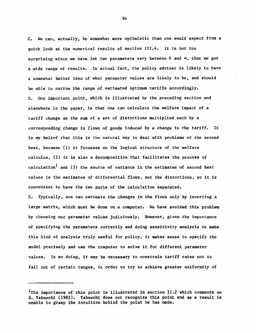
94
C. We can, actually, be somewhat more optimistic than one would expect from a
quick look at the numerical results of section III.4. It is not too
surprising since we have let two parameters vary between 0 and -, that we got
a wide range of results. In actual fact, the policy adviser is likely to have
a somewhat better idea of what parameter values are likely to be, and should
be able to narrow the range of estimated optimum tariffs accordingly.
D. One important point, which is illustrated by the preceding section and
elsewhere in the paper, is that one can calculate the welfare impact of a
tariff change as the sum of a set of distortions multiplied each by a
corresponding change in flows of goods induced by a change in the tariff. It
is my belief that this is the natural way to deal with problems of the second
best, because (1) it focusses on the logical structure of the welfare
calculus, (2) it is also a decomposition that facilitates the process of
calculation' and (3) the source of variance in the estimates of second best
values is the estimates of differential flows, not the distortions, so it is
convenient to have the two parts of the calculation separated.
E. Typically, one can estimate the changes in the flows only by inverting a
large matrix, which must be done on a computer. We have avoided this problem
by choosing our parameter values judiciously. However, given the importance
of specifying the parameters correctly and doing sensitivity analysis to make
this kind of analysis truly useful for policy, it makes sense to specify the
model precisely and use the computer to solve it for different parameter
values. In so doing, it may be necessary to constrain tariff rates not to
fall out of certain ranges, in order to try to achieve greater uniformity of
'The importance of this point is illustrated in section II.2 which comments onS. Yabuuchi (1982). Yabuuchi does not recognize this point and as a result isunable to grasp the intuition behind the point he has made.
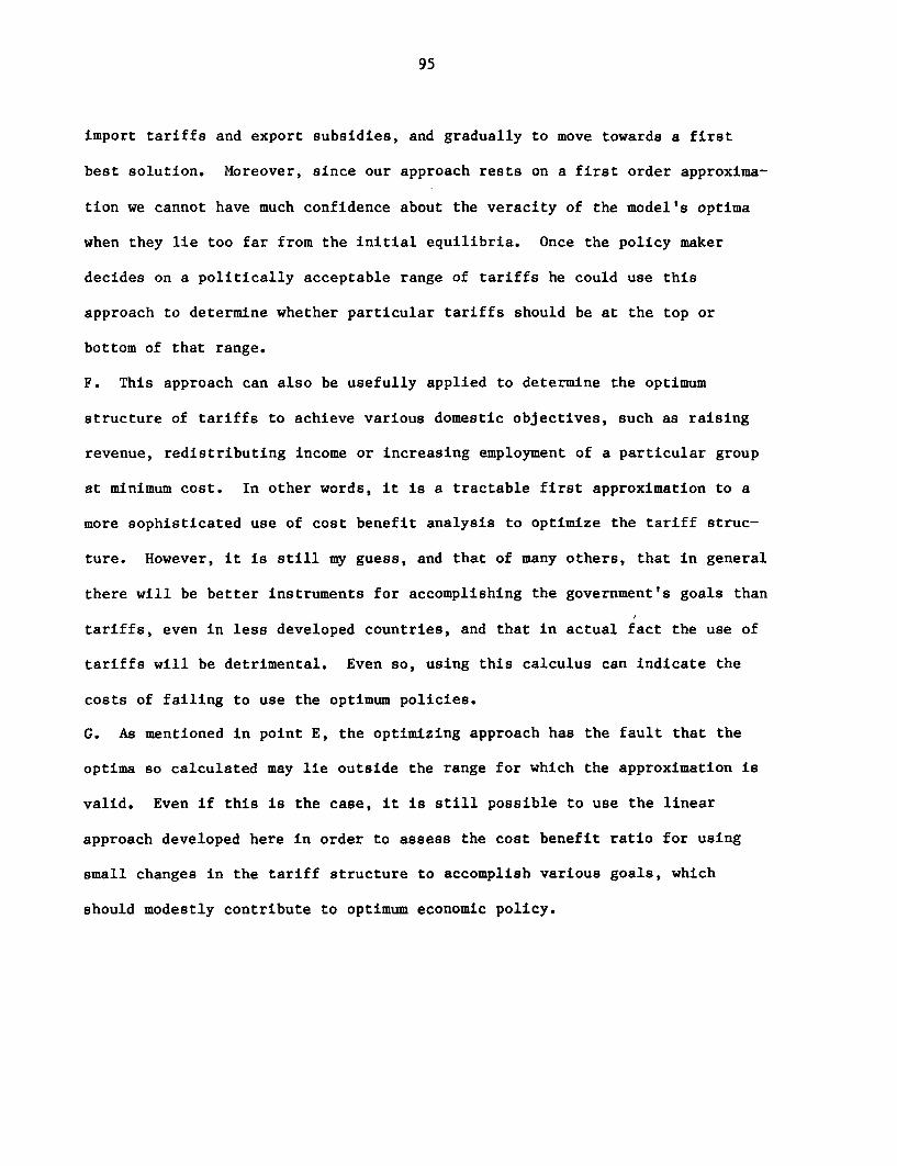
95
import tariffs and export subsidies, and gradually to move towards a first
best solution. Moreover, since our approach rests on a first order approxima-
tion we cannot have much confidence about the veracity of the model's optima
when they lie too far from the initial equilibria. Once the policy maker
decides on a politically acceptable range of tariffs he could use this
approach to determine whether particular tariffs should be at the top or
bottom of that range.
F. This approach can also be usefully applied to determine the optimum
structure of tariffs to achieve various domestic objectives, such as raising
revenue, redistributing income or increasing employment of a particular group
at minimum cost. In other words, it is a tractable first approximation to a
more sophisticated use of cost benefit analysis to optimize the tariff struc-
ture. However, it is still my guess, and that of many others, that in general
there will be better instruments for accomplishing the government's goals than
tariffs, even in less developed countries, and that in actual fact the use of
tariffs will be detrimental. Even so, using this calculus can indicate the
costs of failing to use the optimum policies.
G. As mentioned in point E, the optimizing approach has the fault that the
optima so calculated may lie outside the range for which the approximation is
valid. Even if this is the case, it is still possible to use the linear
approach developed here in order to assess the cost benefit ratio for using
small changes in the tariff structure to accomplish various goals, which
should modestly contribute to optimum economic policy.
96
Chapter IV
ON THE SYMMETRY BETWEEN EFFECTIVE TARIFFS AND
VALUE ADDED SUBSIDIES
IV.1 INTRODUCTION
This chapter is the first of a set of three designed to introduce and
explain the meaning of the concepts of the effective rate of protection (ERP)
and domestic resource cost (DRC) which have been used so extensively in the
World Bank and elsewhere. The problem posed in these chapters is: How should
ERP and DRC calculations be used to make inferences about appropriate economic
policy?
IV.2 ON ALTERNATIVE DEFINITIONS OF THE NOMINAL
RATE OF PROTECTION
Thinking about the effective rate of protection is made difficult by the
fact that the concept of the ERP has been used by different authors to refer
to two different things and sometimes by the same author to refer to different
things. The confusion arises out of the fact that the nominal rate of protec-
tion (NRP) is not unambiguously defined. Corden (1971, pp. 21-25) notes that
one can define the rate of protection as either (1) the proportional differ-
ence between the domestic (p) and foreign (p*) prices of a good, (p-p*)/p*, or
else (2) the proportional increase in the domestic price of a good that
finally results from a protectionist regime. Of course when world prices are
fixed both of these concepts are the same, but generally they will be
97
different. Corden goes on to say (p. 25) "Clearly, which concept one uses
depends on one's purpose, but it is at least worth noting that the term rate
of protection... is not unambiguous. Generally the second meaning of the term
is the one we shall have in mind when considering resource allocation effects
of tariffs, export subsidies, and so on. But for marginal welfare analysis
the first meaning is the relevant one." This is true, and the same ambiguity
applies to thinking about the ERP. I find the definition of the ERP which is
analogous to Corden's first definition of the NRP to be useful because the ERP
defined in this sense plays the role of a subsidy which is useful in the
welfare economics discussed in chapters V and VI. However, I find the second
definition to be much less useful. Thus, this chapter will present my
preferred definition first, show some of what can be done with it and then
criticize the second definition.1 The next chapter will show how to use this
preferred definition to calculate shadow prices.
IV.3 THEOREM AND IMPLICATIONS
There are two useful symmetry theorems regarding tariffs, taxes and
subsidies in international trade. One is the Lerner Symmetry Theorem which
states that across the board taxes on imports and across the board taxes on
exports have identical effects.2 The second is the proposition that an import
tariff may be viewed as a combination of a consumption tax and a production
'Some authors are inconsistent in their definitions. For example Johnson(1971) used different definitions on p. 310 and p. 334 which are analogous toCorden's first and second definitions of the NRP respectively.
2For discussion of this and related theorems see Kaempfer and Tower (1982).
98
subsidy.3 In this chapter we prove a third symmetry theorem closely related
to the second:
Consider an economy which uses intermediate inputs in fixed proportions
along with primary factors to produce outputs. In such an economy, there
is an equivalence between two fiscal structures. One is the levy of a
vector of tariffs on net imports, where these tariffs are expressed as
fractions of world prices. The other is the levy of a set of consumption
taxes (expressed as fractions of prices to sellers) equal to that set of
nominal tariffs combined with a set of subsidies to value added (expressed
as a fraction of gross value added), equal to the effective rates of pro-
tection which the nominal tariffs imply, where these ERP's are calculated
as the proportion by which unit value added at domestic prices exceeds
unit value added at world prices, with both measures determined using the
domestic physical input/output coefficients.
This theorem is rather general, for it holds in both barter and monetary
economies and it holds regardless of whether the market structure is
competitive abroad or whether or not world prices are fixed, and to a limited
extent even if domestic markets are not competitive. It is also a theorem
which is closely related to statements in the literature.4 Still, it has
3See for example Harry G. Johnson (1965). Gene Grossman has pointed out to methat this theorem also holds in the presence of imperfect competition ormultiple imperfect competitors, just as the Lerner Symmetry Theorem does. Forthe logic of this proposition in the context of the Lerner Symmetry Theorem,see Kaempfer and Tower (1982) and Eaton et al. (1982).
4See, for example, Corden (1966) and (1971). Also, Harberger (1974, p. 75) notesthat if intermediate inputs are combined in fixed proportions to produce output,there is an equivalence between any given set of taxes on intermediate inputs andoutput on the one hand and a tax on value added on the other. The reason that ithas not been stated explicitly before is, I believe, because the vast majority ofauthors have used the definition of the ERP for conceptual purposes which isanalogous to Corden's second definition of the NRP, even though in performingcalculations they define the ERP as we have defined it.
99
never been stated, and I believe it provides a useful way of looking at the
ERP.5
Moreover, the theorem has an important corollary which is:
A vector of tariffs on net imports combined with the same vector of
consumption subsidies (expressed as fractions of the prices to con-
sumers) and taxes on value added (expressed as fractions of disposable
factor incomes) equal to the implied ERPs will be equivalent to free
trade.
From a policy standpoint, the corollary is very important. Missions from
the World Bank frequently calculate effective rates of protection. But ERPs
have fallen into ill repute in some quarters because they are imperfect
indicators of how freeing up trade would move resources or affect economic
welfare.6 But this is not a proper reason to reject such calculations,
because after all even when there is no input-output structure, tariff changes
are not perfect predictors of welfare changes or resource movements,7 yet it
is useful to know what tariffs are for they are essential inputs into any
general equilibrium calculation. Similarly, ERPs play an important role in
many general equilibrium calculations designed to reach conclusions about both
welfare and resource allocation,8 for they can be thought of as implicit
subsidy rates on value added, and hence the distortion associated with employ-
5Note that we are pretending here that the value added tax or subsidy isneither charged on imports nor rebated on exports, although countries withvalue added tax tend to do this in practice. For more on this see McKinnon(1971).
6For example, see Ray (1973, p. 256).
7For example, consider the Metzler paradox which implies that cutting theimport tariff may cause the level of imports to fall.
8See, for example, Bertrand (1972), Pursell (1978) and Tower and Pursell(1984).
100
ment of resources in a particular activity.
I conclude, therefore, that policy advisors may find it helpful to
interpret ERPs to authorities in the LDCs which they advise as the equivalents
of value-added subsidies, and the normative significance they should attach to
differential ERPs is precisely the normative significance that one would
attach to differential subsidies and taxes on value added in different sec-
tors: namely a value-added subsidy is the amount by which the wage received
by the suppliers of factors exceeds the wage paid by demanders of factors.
Competition causes the supply prices of the same factor in all industries
to be the same. Therefore, differential subsidies to value added will cause
the subsidy-inclusive costs of the same factors to different demanders to
differ by the subsidy differential. Thus we can treat the ERP as the distor-
tion associated with the production of value added, which means that the
policy maker need only point out that differential ERPs are production
distortions, and that to eliminate the distortions on production, differential
value-added taxation can be used to offset completely the ERPs, and similarly
to eliminate the distortions on consumption, differential consumption subsi-
dies can be used to offset completely the nominal tariffs. Moreover, such a
complete offset occurs when consumption subsidies (as a fraction of the prices
to consumers) are levied at the nominal tariff rates and value added in all
industries is taxed at a rate (as a fraction of disposable income) equal to
the effective rate of protection.
101
IV.4 DEFINING THE ERP AND EXPLORING ITS
RELATIONSHIP TO THE NRP
We continue to use the conventional assumption that intermediate inputs
and a value-added aggregate are combined in fixed proportions and with
constant returns to scale (CRS) to produce output, and that the value-added
aggregate is itself a CRS aggregate of primary factors (e.g. capital and
labor).
Given our assumed production relationship, any activity can be thought of
as the production of a basket of various goods in fixed proportions, where
some of the goods are present in the basket in negative quantities - i.e. as
inputs. The value of the basket in world prices is simply value added
measured in world prices. Similarly, the value of the basket in domestic
prices is simply value added in domestic prices.
Corden's first definition of the NRP of a good is simply the proportion
by which its domestic price exceeds its world price. If the good is an
importable, this is simply the nominal tariff rate expressed as a fraction of
the world price, and if it is an exportable it is simply the export subsidy
again expressed as a proportion of the world price. By analogy, we choose to
define the ERP as simply the proportion by which the domestic price of the
basket exceeds the world price. The ERP for an activity then is in this sense
the average tariff on the particular commodity basket produced by that
activity. Therefore, it is not surprising that it plays a role which is
similar to that of the NRP. Moreoever, in the special case where there are no
intermediate inputs, this definition boils down to that of the NRP.
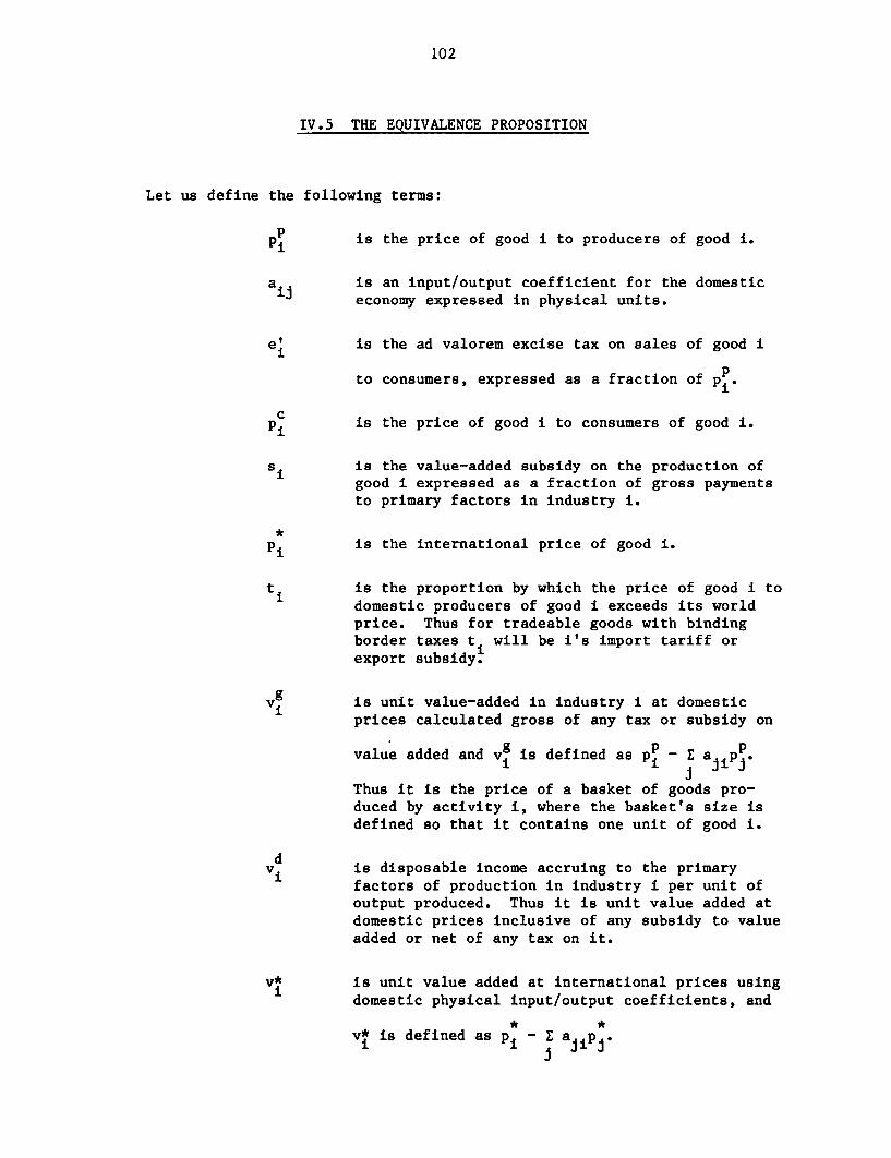
102
IV.5 THE EQUIVALENCE PROPOSITION
Let us define the following terms:
is the price of good i to producers of good i.
aij is an input/output coefficient for the domesticeconomy expressed in physical units.
el is the ad valorem excise tax on sales of good i
to consumers, expressed as a fraction of pip.
c~~~~~~~~~~~~~~~~p c is the price of good i to consumers of good i.
si is the value-added subsidy on the production ofgood i expressed as a fraction of gross paymentsto primary factors in industry i.
Pi is the international price of good i.
t i is the proportion by which the price of good i todomestic producers of good i exceeds its worldprice. Thus for tradeable goods with bindingborder taxes ti will be i's import tariff orexport subsidy.
Vig is unit value-added in industry i at domestici prices calculated gross of any tax or subsidy on
value added and vi is defined as p E ajiPiJ
Thus it is the price of a basket of goods pro-duced by activity i, where the basket's size isdefined so that it contains one unit of good i.
v d is disposable income accruing to the primaryvi factors of production in industry i per unit of
output produced. Thus it is unit value added atdomestic prices inclusive of any subsidy to valueadded or net of any tax on it.
vg* is unit value added at international prices usingi domestic physical input/output coefficients, and
V* is defined as P E ajiPi jij
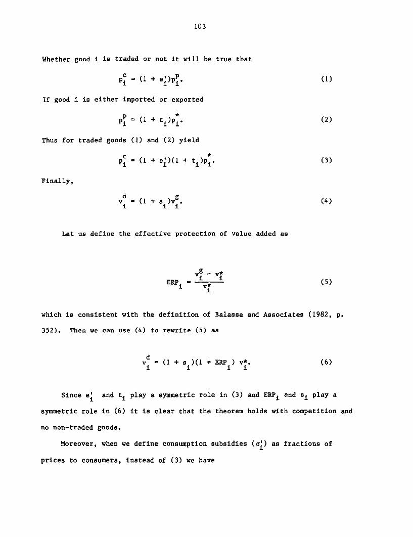
103
Whether good i is traded or not it will be true that
piC =(1 + e )pP. (1)i ii
If good i is either imported or exported
PPi =(1 + t )pi. (2)
Thus for traded goods (1) and (2) yield
c *P= (1 + e')(1 + t )p1. (3)
Finally,
d g= (1 + s )v *(4)
i i i
Let us define the effective protection of value added as
v9 - v*
ERP = Vi* (5)
which is consistent with the definition of Balassa and Associates (1982, p.
352). Then we can use (4) to rewrite (5) as
dv ' (1 + s )(1 + ERP ) V*. (6)
Since ei and ti play a symmetric role in (3) and ERPi and si play a
symmetric role in (6) it is clear that the theorem holds with competition and
no non-traded goods.
Moreover, when we define consumption subsidies (a) as fractions of
prices to consumers, instead of (3) we have
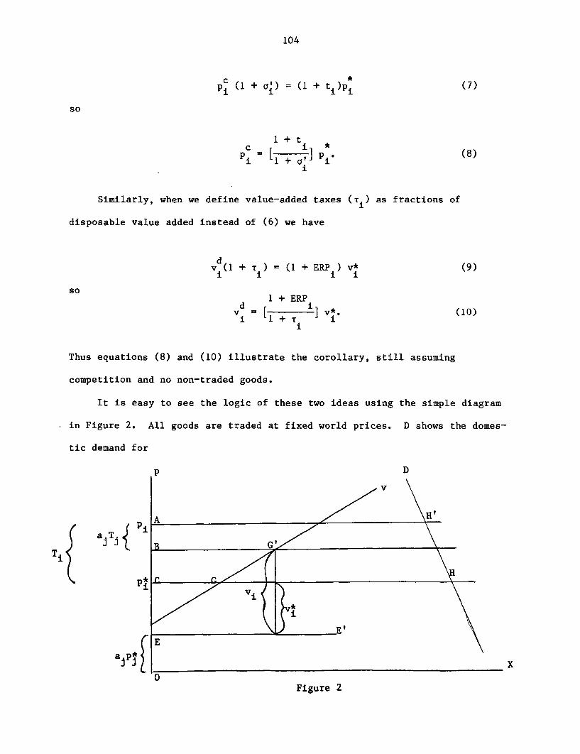
104
PC ( + ai) (1 + (7)
so
I + tc ~~i *
Pi I+ i p. (8)
Similarly, when we define value-added taxes (T.) as fractions of
disposable value added instead of (6) we have
v (1 + Ti) = (1 + ERP ) V* (9)i ii i
so1 + ERP
d iv = I[ + ] V i. (10)
i
Thus equations (8) and (10) illustrate the corollary, still assuming
competition and no non-traded goods.
It is easy to see the logic of these two ideas using the simple diagram
in Figure 2. All goods are traded at fixed world prices. D shows the domes-
tic demand for
P D
Figure 2
105
the good in question. The only input is good j, and aj is its input coef-
ficient. Thus EE' shows the cost of the sole intermediate input per unit of
output at world price. v is drawn with respect to EE' as the horizontal axis
and is the supply curve of value added. In free trade domestic output is at G
with consumption at H. A tariff on the import of i raises domestic price by
AC to A so that consumption falls to H', which is just as if a consumption tax
of AC had been imposed. The import tariff on j, Ti, raises unit costs by AB,
so the net increase in unit value added at domestic prices is only BC. This
means that production equilibrium moves to G', with unit value added at domes-
tic and world prices given by vi = BE and v* = CE respectively. Thus, the ERPi ~~~i
is given by BC/CE. However the same result could have been brought about by
free trade combined with a proportional subsidy to gross value added (i.e.
value added before the subsidy) of BC/CE. Thus the equivalence is estab-
lished. Similarly an import tariff on i of AC combined with a consumption
subsidy of AC restores consumption to H, while our set of tariffs combined
with a tax on unit value added of BC restores production equilibrium to G, and
this establishes our neutrality proposition.
IV.6 ADDITIONAL EQUIVALENCE PROPOSITIONS
There are two additional equivalence propositions which further clarify
the meaning of the ERP, although they are not as useful as the ones we have
just discussed. We have defined the ERP as the wedge between the domestic
price of a sector's basket of goods and world price created by the tariff
structure. It is a small additional step to note that if all of a sector's
inputs and outputs were subject to an import tariff or export subsidy equal to
the ERP calculated from the existing tariff structure, instead of their actual
106
tariffs, no real variables would change. Thus the ERP is the average tariff
on an activity's inputs and outputs. This gives us equivalence proposition 2:
Consider an economy which uses intermediate inputs in fixed propor-
tions along with primary factors to produce outputs. In such an economy,
there is an equivalence between two fiscal structures. One is the levy
of a vector of tariffs on net imports, where these tariffs are expressed
as fractions of world prices. The other is the levy of a set of
consumption taxes (expressed as fractions of prices to sellers) equal to
that set of nominal tariffs combined with a set of taxes on each sector's
inputs and subsidies on its outputs (expressed as a fraction of world
prices) equal to its effective rate of protection.
Moreover, we can come up with an equivalence proposition that holds even
when there is substitution in use of intermediate inputs equivalence
proposition 3:
Consider an economy which uses intermediate inputs in variable pro-
portions but with constant returns to scale along with primary factors to
produce outputs. In such an economy, there is an equivalence between two
fiscal structures. One is the levy of a vector of tariffs on net
imports, where these tariffs are expressed as fractions of world prices.
The other is the levy of a set of consumption taxes (expressed as frac-
tions of prices to sellers) equal to that set of nominal tariffs combined
with a set of subsidies to value added equal to the ERPs and a set of
taxes on each of a sector's net inputs equal to the initial tariff minus
the sector's ERP.
Thus, the ERP still has a meaning as an indicator of incentives even with
107
substitution between intermediate inputs,9 but it is questionable whether any-
one would find the concept very useful in these circumstances.
IV.7 THE EFFECTIVE RATE OF VALUE ADDED SUBSIDY AND
THE IMPLICIT RATE OF FINAL DEMAND TAXATION
From the standpoint of policy modeling perhaps the most important divi-
dend of this discussion is that one can write the relationship between world
prices and prices to final demanders of traded goods as
Pi ' (1+Ti)pi (11)
and label Ti as the implicit rate of final demand taxation, because it is the
proportion by which prices to final demanders are raised above world prices by
the tax and tariff structure.
Similarly,
dvi (l+zi)v* (12)
where zi is the effective rate of value added subsidy because it is the amount
dby which disposable value added, vi , exceeds what it would be if inputs and
outputs were evaluated at world prices, v*. Substituting from (3) and (6)i.
into these equations yields expressions for these two rates:
9For a crystal clear discussion of the relationship between the "true" and the"measured" ERP when there is substitution between primary and intermediateinputs which corrects and clarifies earlier proofs by Corden and Finger seeDutton and Stoeckel (1982).
108
T= (l+ej)(l+ti) 1 (13)
and
Zi = (1+si)(1+ERPi) - 1. (14)
Since the incentive system can be completely described by our Ti's and zi's,
these last two formulae are useful summaries of the incentives yielded by any
tax or tariff system for use in policy analysis.10
Finally, it is important not to focus solely on the effective subsidiza-
tion of value added to the exclusion of implicit final demand taxation. It is
important to know both things in order to fully describe the incentives
present. Since there is more scope for specialization in production than in
consumption the former are more important than the latter, but it would be a
mistake to entirely ignore the latter.
IV.8 NON-TRADED GOODS
Non-traded goods as inputs and/or outputs create no problem for our
equivalence propositions. If they are potentially tradeable, our equations
hold with ti defined from equation (2) as (pp - the wedge between
lCorden (forthcoming) notes that ERPs sometimes take into account consumptiontaxes and subsidies on inputs as well as production taxes and subsidies. Wehave defined our ERPs to exclude consumption taxes, but to include subsidieson intermediate inputs, while we have included explicit value added taxationin our zs but not our ERPs. Yet another option would be to include consump-tion taxes on the good itself in calculating the ERP on production for thehome market. Then for each exported good one would calculate two ERPs, onefor home consumption and one for export. If one also incorporated explicitvalue added taxes and taxes on the use of intermediate inputs, then the sym-metry theorem would be further simplified; there would be symmetry between theexisting structure of taxes, tariffs and subsidies, and an alternativeconsisting of a set of value added subsidies equal to the calculated ERPscombined with taxes on imported consumption goods equal to the differencebetween consumer prices and world prices.
109
domestic producer prices and world prices.
Finally, for both truly non-traded goods, which would not be traded, even
in the absence of trade barriers and for potentially tradeable goods, we have
four obvious options.
8.a The 'Sophisticated' Corden Method
The first option is to treat any production process along with its asso-
ciated non-traded inputs as an integrated production process which uses traded
inputs and primary factors to produce outputs. This is the Corden method
(referred to by Little, Scitovsky and Scott, 1970, as the 'sophisticated'
Corden Method to distinguish it from the 'crude' Corden Method explained
below) of treating non-traded goods and is described in Balassa and Associates
(1982, pp. 352-3). Then in defining the ERP of a non-traded good, i, which is
*pconsumed domestically we can set pi = piE. In this case, assuming zero initial
consumption taxes, the observed tariff structure is equivalent to
(1) a set of consumption taxes on tradeables equal to that set of nominal
tariffs, plus
(2) zero consumption taxes on non-tradeables plus
(3) a set of subsidies to value added in the integrated tradeables industries
equal to their ERPs plus
(4) a set of subsidies to value added in the integrated non-tradeables
industries which produce solely for domestic consumption equal to their
ERPs. Thus, in this scheme, production of a non-traded good which uses no
non-traded inputs, and is both consumed directly and used as an input into the
production of another good is counted both as one production process and as
part of another.
110
8.b The Balassa Method
A second option for treating non-traded goods is the Balassa method
described in Balassa and Associates (1982, pp. 352-3). Using this method we
define the Balassa ERP by (5) with the terms in the right hand side of (5)
defined as* * *
v + Hi p -E a p (15)
and
v9 + H p -Ea ,p (16)i i i j i i i
d g where we assume away value added taxation so that vi v= vi= s aji consists
of the physical measure of the jth tradeable used directly in producing a unit
of i and indirectly in producing the non-tradeables that go into producing a
unit of i; Hi is value added in producing non-tradeables (home goods) used
directly and indirectly in producing a unit of i; and vi and vi refer to
value-added in the ith industry narrowly defined, i.e. not vertically
integrated as in the Corden method.
Then using (4) and (5) we can produce (6) as before, which indicates the
symmetry between the Balassa ERP and value added subsidization. Thus, if we
* * p* Pobserve a particular set of vi, Hi, vi , Pi, Pi, i aj p , E a p, for some
i, and are told there are no value added taxes, we can calculate the Balassa
ERP associated with it. If, alternatively, we are confronted with the same
data and are told that there are no tariffs and no value-added taxes on
intermediate non-traded goods, we can calculate the value added subsidy on
good i which is consistent with the data, and this subsidy will be the Balassa
ERP for good i.
Thus the Balassa ERP for good i is the subsidy to value added on i which
has the same impact on all real variables as the tariff on i and on its direct
III
and indirect inputs, under the assumption that there is no value added
taxation on the non-tradeables which feed into the tradeables.
Clearly then, there is a symmetry between a set of tariffs and zero
consumption taxes on the one hand and on the other
(1) a set set of consumption taxes on tradeables equal to the nominal tariffs
plus
(2) zero consumption taxes on non-tradeables plus
(3) value added subsidies equal to the Balassa ERPs on the production of both
all tradeables and those non-tradeables which are directly consumed plus
(4) zero value-added subsidies on non-tradeables used as intermediate inputs.
8.c The 'Crude' Corden Method
A third option for treating non-traded goods is the 'Crude' Corden method
described in Little, Scitovsky and Scott (1970, p. 431-2). Using this method
we define the crude Corden ERP (ERPCC) by (5) with the terms in the right hand
side of (5) defined as
* * *
vi Pi- ajPj (17)
and
Vi a Pp - iajpp (18)
where aji consists of the physical measure of the jth tradeable used directly
in producing a unit of i. Thus in this method we treat non-tradeable inputs
into i just like primary factors in calculating value added and hence the
ERP. The difference between this method and the 'sophisticated' Corden method
is that in the former we do not net out traded inputs into non-traded goods in
calculating value added.
112
With this definition, there is a symmetry between a set of tariffs and
zero consumption taxes on the one hand and on the other
(1) a set of taxes on traded goods consumed or used as inputs into non-
tradeables equal to the nominal tariffs plus
(2) zero consumption taxes on non-tradeables plus
(3) subsidies on the use of primary factors and non-traded goods to produce
traded goods equal to the Crude Corden ERPs plus
(4) zero subsidies on goods and factors used to produce non-traded goods.
The reader should note that these definitions of the Balassa and Corden
methods deviate a bit from those authors' definitions, because in their work,
their reference prices are free trade prices rather than world prices. Our
procedure has been to choose definitions that fit the symmetry theorems.
8.d The Simple Balassa Method
A fourth option, labeled by Corden (1975, p. 64) the simple Balassa
Method, is perhaps the simplest and most reasonable choice in many cases. This
is to set P PP for all non-traded goods in the calculation of effective
protection of all traded and non-traded goods. 1 1 In words, the reference
price for each non-traded good is simply the price which the domestic producer
receives for it. Then we treat an excise tax on the sale of the jth good to
the ith producer just like a tariff on the jth good in calculating the ERP on
i. Thus the ERP on a non-traded good which uses non-traded goods as its sole
inputs would be the (negative) value-added subsidy which is equivalent to the
excise taxes paid on its intermediate inputs of non-traded goods. Corden
"lThe analysis of the next section finds this procedure to be useful. Cordennotes that the simple Balassa (1965) method groups non-traded inputs withtraded inputs, and treats the former as if they were traded inputs with zerotariffs. He also notes that Balassa has since abandoned use of this method.
113
(forthcoming) notes that we can define a scale of ERPs for all tradeables, but
this fourth definition enables us to calculate an ERP for each traded and non-
traded good, and in calculating these ERPs one need look only at direct
inputs. Thus, in contrast to the other three methods, no matrix inversion is
required.12 The symmetry theorem which emerges in this case is simply the one
noted in the introduction of this section.
Finally, selecting a reference price of pp for non-traded goods is com-
pletely arbitrary. The symmetry and neutrality theorems will hold regardless
of what price is selected. -It is just that when a higher reference price for
good i is selected, the ERPs for goods which use i as an intermediate input
will be larger and the ERP for good i will be lower than they would otherwise
be.
We defer until the next section a discussion of the normative signifi-
cance of ERPs defined in this way. For the time being, we merely note that
these ERPs represent wedges rather than measures of incidence. For example if
an intermediate non-traded input is provided inelastically with nontaxed
intermediate inputs, and it is taxed, production of that good would bear the
incidence of the tax, although the tax would leave its ERP as we propose to
calculate it still at zero and would reduce the algebraic value of the ERPs of
the sectors which use it.
12Balassa and Associates (1982, p. 353) note, however, that "In practice, anapproximation can be used instead of the (partial) inversion of the input-output matrix."
114
IV.9 MONOPOLY POWER
Now, so far we have ducked the problem of monopoly power. Imperfect
competition in the home economy will destroy the symmetry of the theorem in
its most simple form. The problem is that if the monopolist-monopsonist is
not a price taker in either his output market or the market for his inter-
mediate inputs, a given set of nominal tariffs will generate different levels
of the calculated ERP depending on what level of output the monopolist-
monopsonist chooses. Thus, for the monopolist-monopsonist, ERP will be a
function of his level of output:
ERPi = ERPi(Qi). (19)
Accordingly, for our monopolist-monopsonist, a symmetry emerges, but it is a
symmetry between the effective rate of protection and a subsidy to value-added
which has the same functional dependence on output that ERP does:
Si = ERPi(Qj). (20)
In the special case where our monopolist-monopsonist is unable to influence
the price of any of his traded inputs or the price of his output and non-
traded goods are handled using the Corden method, it is not necessary to
reckon with the monopoly-monopsony behavior explicitly, and the symmetry
theorem which holds under competition continues to hold under monopoly.
115
IV.10 ABSOLUTE LEVELS OF NOMINAL AND EFFECTIVE PROTECTION DON'T MATTER
If we ignore capital flows between countries, pretend that either the
exchange rate or wages and prices are perfectly flexible, and assume that the
government's real budget surplus is kept constant by a variable neutral income
subsidy, absolute domestic prices cease to play a role, and only relative
domestic prices matter. In that circumstance, any fiscal structure (set of
e's, t's, s's and ERPs) will be equivalent to any initial fiscal structure
(set of e's, t's, s's and ERPs ) so long as relative prices stay unchanged,
i.e. from (3) and (6) so long as for all i
(1+e')(1+t ) = a(l+e)(1+t i) and (1+s i)(1+ERP i) 0(1+si )(1+ERPi) (21)
where a and $ are arbitrary positive factors of proportionality. Thus, for
example, we can double the 'force"13 of each ERP and nominal tariff and/or
triple the force of each excise tax without affecting any economic variable.14
13Bacha and Taylor (1971, p. 202) define the force of x as 1 + x.
14The reason that absolute levels of ERPs don't matter is identical to thereason that the level of prices don't matter in a simple world where wages andprices are flexible, namely that a proportional increase in the money stockwill cause all prices to rise by the same proportion, leaving all relativeprices unchanged. However, if there were minimum nominal wages, uniformlyhigher ERPs could raise prices and consequently raise real output levels.Similarly, if there were specific consumption taxes, the inflation generatedby uniformly higher ERPs could erode their real value and change real incomes.Finally, international factor mobility will generally invalidate the proposi-tion, for if one country's residents hold wealth denominated in the othercountry's currency, a uniform increase in domestic ERPs will raise domesticprices and cause domestically owned wealth measured in domestic goods to fall.
However, the proposition also applies even in the presence of interna-tional factor mobility and international trade in services so long as theimport or export of factors or services is treated just like the import orexport of goods and whatever tariff changes apply to goods apply to them aswell. For more on this, see Kaempfer and Tower (1982).
116
This means that policy advisors when talking with clients should emphasize
that uniformly positive ERPs mean only that domestic prices will be absolutely
higher than foreign ones, but in a barter world or in a non barter world in
equilibrium with no price rigidities, the only thing that matters is percent-
age differentials between the forces of the ERPs.15
IV.11 THE NET EFFECTIVE RATE OF PROTECTION
This idea has led Corden (1966) to introduce the concept of the net
effective rate of protection, NERP, where the net ERP is simply the propor-
tional change due to the tariff structure in value added measured in units of
a basket of non-traded goods. Thus, the NERP is a device for normalizing
ERPs. In general the choice of the basket of goods to use as numeraire is
somewhat arbitrary. However, in the special case where value added in every
sector is produced with one sector specific factor and a common mobile factor,
the services of the mobile factor is the natural choice for numeraire, for
then the mobile factor will have moved in or out of the sector in accordance
with whether the sign of the NERP is positive or negative.
Corden and Balassa (1982, p. 353) describe the NERP as correcting for the
currency appreciation which typically accompanies the imposition of a tariff
15Corden (1984) and others also note that what matters is non-uniformity inthe scale of ERPs. As an aid in understanding the differences between theCorden and Balassa ERPs, note that a system of uniform import tariffs andexport subsidies of x% will result in no resource misallocation, but CrudeCorden and Sophisticated Corden ERPs for all tradeables will be calculated asx%, while either of the Balassa calculations would yield ERPs of tradeablegoods of less than x%. Similarly, a proportionate increase in the forces ofall import tariffs and export subsidies which would have no implications forresource allocation would result in the same proportionate increases in theforces of all Crude and Sophisticated Corden ERPs for tradeables, but that isnot true for either of the Balassa measures. Finally, the force of the ERP issometimes referred to as the ERP coefficient.
117
structure. I think this is confusing however, because the appreciation that
occurs depends on which basket of goods has its domestic currency price held
constant by domestic monetary policy, and this is arbitrary.
It should be noted that in applying Balassa's equations (13) and (14) on
page 354 to calculate NERPs requires that the ERPs with which they are used be
calculated as the proportional difference between value added in domestic
prices in the post-tariff situation and at world prices under free trade, not
world prices in the tariff situation. This is because (13) and (14) assume
imperfectly elastic foreign excess demands and supplies. However, to calcu-
late ERPs defined with reference to free trade world prices from data applying
to the protected equilibrium, when world prices are variable may be a complex
process.
Finally, Corden (1971, p. 162) discusses yet another way of treating non-
traded goods called the Scott method, which requires treating non-traded goods
as other traded goods in calculating value added where in calculating ERPs,
the increase in the domestic price of the non-traded good due to the tariff
structure is treated just like a tariff which raises the domestic price of a
traded good. Denoting N as the proportional increase in the price of the non-
traded good due to the tariff structure, and ERPs as the Scott measure of the
ERP of a good, we can solve for the net ERP as
1 + NERP = 1+ERPs1+N
Thus, the relationship between the Scott method and the NERP is very close.
Both are attempts to solve the general equilibrium problem, and while the
numeraire in the Scott method is world prices, in the NERP it is the price of
some bundle of non-traded goods.
118
IV.12 NEGATING THE REAL IMPACT OF A TARIFF STRUCrURE
Similarly, equations (8) and (10) indicate that proportionality between
consumer prices and world prices and between domestic and world value added is
maintained which means that there are no consumption or production distortions
so long as for all i
1 + t 1 + ERPi i
- = y and i = e (22)1 + °i 1 + Ti
i i
where y and e are arbitrary positive factors of proportionality.
Thus it is possible to offset completely the consequences for resource alloca-
tion and hence real income of an existing tariff structure with various sets
of consumption subsidies and production taxes so long as the forces of the
consumption subsidies are proportional to the forces of the nominal tariffs
and the forces of the value added taxes are proportional to the forces of the
effective tariffs.
IV.13 ON NEUTRALITY WHEN THERE IS SUBSTITUTABILITY
BETWEEN INTERMEDIATE INPUTS
We have established that when intermediate input coefficients are fixed,
the effects of a tariff structure on production can be completely offset by
taxing value added at a rate equal to the ERP. What happens when there is
substitutability between intermediate inputs? Is there an analogous theorem?
The answer is yes.
Suppose there is substitutability between intermediate inputs. Moreover,
119
suppose that the tax authority calculates the ERP for each firm and imposes a
tax, T, on its value-added equal to its ERP. This means that we have
dV (1+T ) = p - E a p (23)
i i i j jii
and
p - a pi jiiiJI ; T (24)
i p* a p*i I ji j
Combining (23) and (24) yields
dv = p* - E a p*. (25)
i i i ii J
Thus, we see that with value added taxed at the ERP, disposable value added
depends solely on input coefficients and world prices. Thus the firm will
select a level of output and blend of inputs which is independent of the
tariffs it pays on inputs and receives on its output. This is because it
realizes that if it buys more of a heavily tariffed input, its ERP will fall
and consequently so will its value-added tax, leaving it with increased costs
equal to the value of the increased input at world prices.
Clearly then if there are no non-traded goods, we can achieve production
efficiency by taxing value added in each industry at a rate equal to its ERP.
Moreoever, non-traded goods cause no problems. Define p* for non-traded
goods as being equal to p. Then we have a symmetry theorem which states
There is no economic difference between free trade on the one hand, and on the
other a set of tariffs just balanced by consumption subsidies equal to those
tariffs and value-added taxes levied on each firm (regardless of whether it
120
uses and/or produces tradeable or non-tradeable goods) equal to its own ERP,
and this is true even in the presence of monopoly-monopsony power, variable
world prices, variable input-output coefficients for intermediate goods, a
fixed exchange rate, inflexible factor prices in real or nominal terms and
trade imbalance.
The reason that the symmetry holds even when there is a fixed exchange rate
and inflexible factor prices is that substituting the one policy for the other
causes no nominal price faced by consumers or factors of production to alter.
IV.14 ON DRAWBACKS
Even aside from the formal symmetry developed here, there is an important
moral which emerges. Many countries permit exporters who use imported inputs
to drawback the tariffs they have paid. Generally this is argued to be a good
idea because it restores the competitiveness of the exporters. But there is a
second reason why this is a good idea. It encourages them to choose an import
mix as if they faced world prices rather than domestic prices for those
imports. Thus even if industries were homogeneous entities it would be better
on this ground to offer drawbacks or to tax at ERPs calculated from firm data
than to tax at ERPs based on industry wide data on import use.
Now let us consider the related issue of whether a drawback should be
paid for imported inputs or for both imported inputs and their domestically
produced substitutes.16 If both goods are perfect substitutes the import
tariff will raise the domestic price of the domestic substitute by the amount
of the tariff. Initially, we would expect to see those producers eligible for
16This discussion owes its basic idea to a memorandum by Garry Pursell.
121
the drawback using only the imported good, and others using both imports and
the domestically produced variety. If use of the domestically produced good
becomes eligible for the drawback, those producers which are eligible for the
drawback will be indifferent about whether they use the import or the domestic
good, and may start to use some of the domestic good. The only effect of this
should be to liberate some of the import for use by domestic producers which
are not eligible for the drawback, and thereby change the mix of the two
(identical) goods used as inputs by various producers. There would be no
impact on trade, government revenue or real income of any actor.
In the special case, however, where all domestic use of the imported good
is eligible for the drawback, the effective price of the import to all
consumers will fall to the world price. This means that the domestic price of
the domestic substitute will fall to the world price, if use of the domestic
substitute is not eligible for the drawback, but that in effect production of
the domestic good will be subsidized to the amount of the drawback if its use
too is eligible for the drawback.
If our goal is to minimize the distortionary impact of the tariff system,
the best policy would be to limit total drawback claims for the use of each
good to the value of imports of it, for this would reduce the likelihood of
domestic producers reaping subsidies from the drawback system, and yet it
would reduce costs of inventorying and transport by making goods which are
perfect substitutes equally attractive to these potential users who are
eligible for the drawback.17
17Finally, an alternative, which is just our neutrality theorem once again isthat to make all users of both the foreign good and its domestic substituteeligible for the drawback and to tax domestic production at a rate equal tothe tariff would be equivalent to free trade in that commodity.
122
IV.15 EFFECTIVE PROTECTION AS A VALUE ADDED TAX AND
ITS DMPACT ON THE EXCHANGE RATE
As a further illustration of the importance of viewing the ERP as a value
added subsidy, consider the paradoxical result in Johnson (1966) "that tariff
structures may bring about a situation in which appreciation rather than
depreciation would be necessary to preserve equilibrium under trade liberal-
ization; this possibility is due to the fact that a tariff structure may
impose a tax, rather than provide a subsidy, on particular lines of produc-
tion" (Johnson, 1971, p. 358). The point is that if a tariff is imposed on an
imported intermediate input into production of the sole export, we have in
effect taxed labor's use in producing the export and to restore international
competitiveness, when the tariff is imposed, labor's wage in world prices must
fall; consequently tariff liberalization must be accompanied by a wage hike or
else a currency appreciation if wages are held constant.
IV.16 ON A PROPOSAL TO LIBERALIZE TRADE
Now let us see how some of these ideas can be used to facilitate trade
liberalization. Let us pretend once again that output is produced using
various factors in fixed proportions and initially assume away non-traded
goods. If a country wished to liberalize trade without affecting the income
of any factor adversely it could immediately abolish all import restrictions,
and simultaneously initiate value added subsidies equal to the ERPs while
balancing its budget by using a uniform value added tax which would partially
offset the value added subsidies. Such a policy would result in consumption
gains from trade, without causing any factors to move between sectors.
123
Moreover factor incomes would remain unchanged. If all factors have identical
tastes and unitary income elasticities of demand for all commodities they
would share identical proportional increases in their real incomes. More
generally, so long as the budget shares in consumption of all the factors are
reasonably equal, we would expect all factors to experience roughly the same
proportionate change in real income. Then through time, the country could
move its value-added taxes to uniformity. Probably a reasonable scheme would
be to fix a future time period, say 5 years in the future by which full
equality would be achieved, with 20% of the initial discrepancy in each of the
taxes eliminated in each year of the transition. The policy maker might wish
to leave some leeway so that any industries experiencing excess demand would
have any proposed value-added tax increases accelerated, and conversely any
industries experiencing excess supply would have any proposed value-added tax
cuts accelerated.
Non-traded goods would cause no conceptual difficulties. The only
problem is that to find the level of value added taxation that would freeze
their output levels and hence factor incomes, it would be necessary for the
government to pick norms for disposable factor incomes and be prepared to tax
or subsidize as needed to bring incomes in line with those norms.
Such a proposal would be second best to many that could be devised, but I
believe it would be preferable to the traditional method of tariff reduction
which is to gradually reduce tariffs, and it recognizes that if the policy
maker's goal is to avoid rapid changes in income distribution between indus-
tries, the best policy is value added taxation and subsidization - not
tariffs.
Of course, to the extent that the same domestic and foreign product may
not be perfect substitutes, abolishing tariffs could cause changes in the
124
prices that domestic goods would fetch. Still, we could deal with this
problem as with non-traded goods, namely adjust the value added subsidy.18
IV.17 OTHER DEFINITIONS OF THE EFFECTIVE RATE OF PROTECTION
Throughout this section, we have interpreted the ERP as a measure of the
implicit subsidy to value added. However, other authors have used other defi-
nitions which are analogous to Corden's second definition of the NERP, and
they have used the ERP for other purposes. In this section we examine these
other definitions and uses.
Bhagwati and Srinivasan (1983, p. 127) write:
"The objective of ERP theory, then, consists in devising a concept
of protection that, in the presence of tariff structures involving
the imports of intermediate goods, constitutes in effect an index
that will perform the same tasks nominal tariffs perform in
nominal tariff theory: predicting accurately the changes in gross
output, primary factor allocation, real value added, and/or
nominal value added."
B&S (p. 127 and p. 129) also write:
"Two basic definitions of an ERP index have developed in the
literature. In Gorden 1966 and Anderson and Naya 1969 it is
defined as the proportionate increment in value added per unit
level of an activity brought about by the tariff structure over
its free-trade value, whereas in Corden 1969 and Leith 1968 it is
'8McKinnon (1971, p. 290) also notes that a value added tax is a betterprotective device than a tariff since it avoids the consumption distortion.For more on adjustment assistance see various essays in Bhagwati (1982).
125
defined as the proportionate change (due to the tariff structure)
in the "price" of value added (with the assumption that such a
"price" can be defined meaningfully)."
"The two definitions generally yield different ERP numbers.
However, in the special case of a separable production function
where the intermediates are used in fixed proportion to output,
both definitions amount to the same thing."
Thus, in the B&S view the ERP is interesting only to the extent that it
is correlated with the change, due to the tariff structure, in other variables
of interest. Clearly, if we were to solve a general equilibrium system to
determine the impact of a tariff structure on real incomes of various groups
and levels of outputs in various sectors the concept of the ERP would be
superfluous, and it would be sensible to concur with Dixit (forthcoming,
section 6.2) who writes
"To sum up, Samuelson's dictum about consumer surplus seems to
apply equally well to effective protection: the concept can
safely be used only by those who understand it sufficiently well
to do without it."
Harberger (undated) on the other hand lists the theory of effective pro-
tection as one of the four major developments in economic theory which has
contributed to the changes that took place in the economics profession's view
of the development process in the past few decades. He notes that this is
because "Empirical studies... have shown first how high, typically, the
effective rates of protection are, and second how heavy are the burdens, in
terms of the resulting inefficiency, that many developing countries have, as
it were, imposed upon themselves." He also writes "All the confusion about
126
what the rate of effective protection is can be avoided only by having a uni-
form and general tariff on all imports. So while the first lesson emerging
from effective protection and analysis is "liberalize," the second is, to the
extent that liberalization is incomplete, "equalize" the tariff schedule."
I propose that we drop the use of the ERP as defined in the two senses
considered by B&S, and replace it with the concept of the ERP defined as a
measure of the tax or subsidy incentive to value added discussed earlier in
this section. Then if desired, these incentive measures can be combined with
other parameters to calculate the impact of protection on important variables.
Moreover, the ERP defined in this way is easier to calculate and I suspect
will be correlated almost as closely in most circumstances with variables of
importance as the B&S definitions. Of course when world prices are fixed,
there are no non-traded goods and the value added aggregate and intermediate
inputs are used in fixed proportions all of these definitions are the same.
Kreinin, Ramsey and Kmenta (1971) define two broad types of ERP. The
differential form is simply the proportional change in unit value added per
proportional change in the tariff structure while the discrete form is the
proportional change in unit value added brought about by the tariff structure.
They also note that one might consider the alternative of defining effective
tariff rates with respect to variables other than unit value added, and they
define various effective rates of protection as the proportional change in
total value added, output, labor input and profits, using Cobb-Douglas and CES
functions to provide exact expressions for them.
Finally, Hartigan (forthcoming) has defined the ERP for particular
factors or aggregates of factors as the proportional increase in their
utilities due to the tariff structure.
Thus, there are many definitions of the ERP in use and one must be care-
127
ful to define what he means when using the term. Perhaps the bottom line is
that one should be more concerned with the analysis of the effects of protec-
tion than the concept of effective protection in the B&S senses.
IV.18 CONCLUSION
To conclude, whereas many like Ethier (1977) have searched for analogies
between effective and nominal tariffs, the more appropriate analogy is between
the effective tariff and the value-added subsidy. Perhaps we should even
rename the effective tariff, the implicit value-added subsidy.19 In fact
Johnson (1971, p. 312) in a chapter which is a reprint of a 1964 lecture
refers to the ERP as "the implicit rate of protection." The problem is that
"effective" is defined by Webster as "operative" or "actual," which to me
refers to the ultimate consequences of protection after a new general equilib-
rium has worked itself out, whereas "implicit" is defined as "capable of being
understood from something else though unexpressed," which seems to fit the
symmetry concept better.
19Balassa (p. 17 of Balassa and Associates 1982) calls the ERP, calculated asthe proportional difference in value added at domestic and world prices "thepartial equilibrium effective rate."
128
Chapter V
THE IMPLICIT RATE OF FINAL DEMAND TAXATION AND THE EFFECTIVE
RATE OF VALUE ADDED SUBSIDY AS DETERMINANTS OF SHADOW PRICES
V.1 INTRODUCTION
The previous chapter developed the concepts of the effective value added
subsidy, z, and the implicit rate of final demand taxation, T. Now we turn to
the problem of assessing the normative significance of these tools. Bertrand
(1972) derives a simple expression for the effects of shifts in consumption
and production between sectors on economic welfare in which the tariff and the
effective rate of protection play important and symmetric roles. This chapter
accomplishes several things. (1) We rewrite Bertrand's formula in a way that
is easier to understand and interpret. (2) We permit the existence of expli-
cit value-added and sales taxes so that our z replaces the ERP and our T
replaces the tariff in Bertrand's formula. (3) We show that the existence of
non-traded goods and variable world prices leaves Bertrand's formula unchanged
if we replace the T and z with T and z where T is defined as (pi-Pi)/;, where
Pi is the price to domestic consumers and Pi is marginal revenue or marginal
expenditure on world markets if the good is traded or else price to the
'This chapter was suggested by Balassa's (1971, p. 318) observation that wecan "reinterpret the effective rate of protection as a measure of the cost offoreign exchange i.e., the amount of domestic resources (value added) spent tosave (or earn) a unit of foreign exchange." Also see Balassa and Schydlowsky(1972), Bertrand and Vanek (1971), Bruno (1972), Krueger (1972) and Pearson(1976) as well as Ray (1980) which covers much of the same ground as Bertrand(1972). In fact Ray's equation (16) is identical to Bertrand's (15) althoughRay doesn't reference Bertrand's paper.
129
producer of the good if it is non-traded, and zi is the proportion by which
disposable value added in sector i exceeds value-added evaluated at the pis.
(4) We extend the formula so that it can be used to derive shadow prices of
goods, factors and policy parameters and call it our fundamental equation.
(5) We show how this equation can be used in the Little-Mirrlees procedure of
shadow pricing everything as the amount of foreign exchange it saves, holding
real income constant. (6) We show how similar forms emerge for the fundamen-
tal equation when the reference prices are calculated in several different
ways and thereby generalize the concept of effective protection. (7) We use
the equation to calculate the welfare benefit of removing all of the economy's
distortions, thereby extending a formula of Harry G. Johnson's. (8) We show
how to use the equation to assess the welfare impact of making a number of
simultaneous small adjustments in each of various distortions. (9) We inter-
pret the logic of our analysis geometrically. (10) Finally, we assess the
normative significance of different ways of treating non-traded goods.
V.2 DERIVING THE FUNDAMENTAL EQUATION
Let us first define a reference price, Pi, which for exportables is
simply the marginal revenue from selling abroad, - (p/n*)], with n* > 0i ~~~~~i
being the elasticity of foreign excess demand, or for importables the marginal
expenditure necessary to secure one unit from abroad, p*[i + (I/a*t)] where
a* > 0 is the foreign elasticity of excess supply.2 Thus, for tradeables, the
reference price is the rate at which the country can transform the good in
2In the event that foreign excess demand and supply functions are inter-_ *
related, Pi = pi[l + E wjij as defined in section II1.2's equation (10).j
130
question into foreign exchange. For non-tradeables, pi, is defined as the
pprice received by producers of the good, p i. With these definitions we can
define the consumption distortion on good i as
i
Thus if i is a non-tradeable T i is simply the excise tax on its consump-
tion, while if i is traded at fixed world prices, i is simply the import
tariff, export subsidy, or tariff equivalent of any import quota, for it is
the proportion by which price to consumers exceeds world price.
dAs before disposable value added is v i. Now, however we must define
reference unit value added as unit value added at reference prices:
Vi = Pi - E aji Pj (2)
This enables us to define the value added distortion as
Z- [v - ]Ii (3)
Thus when world prices are fixed and there are no tariffs zi is the explicit
value added subsidy on good i, while if world prices are fixed and there is no
explicit value added tax or subsidy z iis simply ERPi. Therefore, Ti is the
proportion by which the price of a good to consumers exceeds its marginal rate
of transformation into foreign exchange or else its price to producers while
Zi is the proportion by which the price of the commodity basket produced by
the ith sector (which contains inputs in negative quantities) to producers in
that sector exceeds its marginal rate of transformation into foreign exchange
131
or else its price to domestic producers of the various goods in the basket.
Since consumers spend all income, the change in their real income is
given by the changes in their consumption, weighted by the prices they face:
dy = p dCi (4)i i i(
We define the exchange rate as unity and the increase in the rate at
which foreign exchange reserves are used up is given by
F = Z pidMi (5)i
where Mi is net imports of the ith good. Thus if the ith good is exported Mi
is negative.
The change in the total net product of the economy, valued at reference
prices can be written either as the value of increased net output of each good
summed over all goods, E pidQi, or else as the value of a unit basket of goodsi
produced in each sector multiplied by the change in the number of baskets pro-
duced by that sector, E vidXi. Thus
E pidQi = v iidX (6)i
where Qi is net output of good i, i.e. gross output minus the quantity of the
good used as intermediate inputs.
Let Qi be the autonomous increase in government sales of the ith good to
the private sector. Then commodity balance dictates for all i that
dMi = dCi - Qi - dQi. Multiplying by pi, summing over all commodities and
substituting from (6) yields
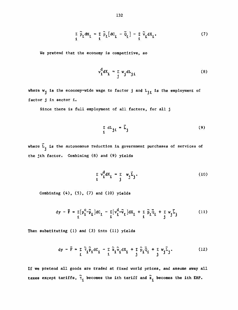
132
E p idMi -=E Pi dC i - Qj-E vi dX1. (7)i i ii
We pretend that the economy is competitive, so
VddX i = dLi (8)
where wj is the economy-wide wage to factor j and Lji is the employment of
factor j in sector i.
Since there is full employment of all factors, for all j
E dLji = L (9)
where L is the autonomous reduction in government purchases of services of
the jth factor. Combining (8) and (9) yields
dE vidXi = E w -L . (10)i i
Combining (4), (5), (7) and (10) yields
dY F i E[P~i Pi ]dC i - E ii-v]dX i + pQi I E jL (11)i i i
Then substituting (1) and (3) into (11) yields
dy - F = E TipidCi - z +vdX, + PQ,+ w1 L; (12)i i j i
If we pretend all goods are traded at fixed world prices, and assume away all
taxes except tariffs, -i becomes the ith tariff and Zi becomes the ith ERP.
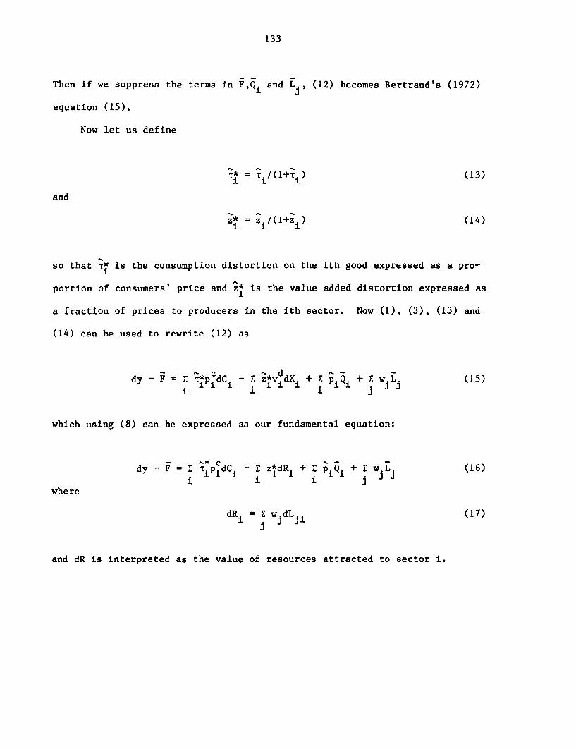
133
Then if we suppress the terms in F,Qi and Li. (12) becomes Bertrand's (1972)
equation (15).
Now let us define
i i i (13)i i
and
i i /( i+~) (14)
so that T* is the consumption distortion on the ith good expressed as a pro-i
portion of consumers' price and Z* is the value added distortion expressed as
a fraction of prices to producers in the ith sector. Now (1), (3), (13) and
(14) can be used to rewrite (12) as
dy - F = E ipdCi z* dXi + i PQi + j j (15), i j
which using (8) can be expressed as our fundamental equation:
dy -F =E ipcdCi E ZdRi +i PQ +Ej j L (16)
where
dRi E widLji (17)a d ii
and dR is interpreted as the value of resources attracted to sector i.
134
V.3 INTERPRETING THE FUNDAMENTAL EQUATION
First, pretend there are no distortions and fixed world prices. Then
(16) tells us that each unit of a good or factor released by the government
will increase real income by the value of that good or factor at domestic
(equal to world) prices. Now lets pretend that the government wishes to
absorb one unit of resources or goods from the private sector, but will then
liberate just enough foreign exchange from its reserves to keep real income
unchanged. Setting dy = 0 in (16) tells us that the requisite foreign
exchange loss is simply the domestic market value of that good or resource.
Now let's focus on the distortions. Suppose that T* is 30% becauseradios
of a 30% import tariff on radios, and t* is -20% because of an export taxrice
on rice, and consider the impact of a small adjustment in excise taxes which
shifts 1$ worth of expenditures away from rice onto radios but leaves
unchanged both resource allocation in distorted sectors and consumption of all
other goods which have consumption distortions. Thus we have
pricedRice = -1$ and p adiosdRadios = +1$, which implies that real incomes
will rise by 50¢ if foreign exchange usage is unchanged, or the requisite
foreign exchange usage necessary to keep the standard of living unchanged
falls by 50¢.
The interpretation of the second term is analogous. Suppose z* isautos
+200% due to a very high import tariff on assembled vehicles and the Zc iscocoa
-50% because of an export tax which keeps its domestic price well below its
marginal revenue in world markets. A change in some sort of taxes whose sole
effect is to shift 1$ worth of resources from autos to cocoa will reduce the
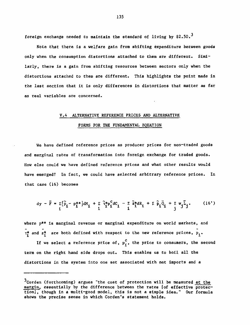
135
foreign exchange needed to maintain the standard of living by $2.50.3
Note that there is a welfare gain from shifting expenditure between goods
only when the consumption distortions attached to them are different. Simi-
larly, there is a gain from shifting resources between sectors only when the
distortions attached to them are different. This highlights the point made in
the last section that it is only differences in distortions that matter as far
as real variables are concerned.
V.4 ALTERNATIVE REFERENCE PRICES AND ALTERNATIVE
FORMS FOR THE FUNDAMENTAL EQUATION
We have defined reference prices as producer prices for non-traded goods
and marginal rates of transformation into foreign exchange for traded goods.
How else could we have defined reference prices and what other results would
have emerged? In fact, we could have selected arbitrary reference prices. In
that case (16) becomes
dy-F = p**]dMi + E T*pdCi iE zdR + E + Q Wj w L (16')i i i j
where p** is marginal revenue or marginal expenditure on world markets, and
T* and z* are both defined with respect to the new reference prices, Pii i
If we select a reference price of, pi, the price to consumers, the second
term on the right hand side drops out. This enables us to boil all the
distortions in the system into one set associated with net imports and a
3Corden (forthcoming) argues "the cost of protection will be measured at themargin essentially by the difference between the rates [of effective protec-tion], though in a multi-good model, this is not a simple idea." Our formulashows the precise sense in which Corden's statement holds.
136
second associated with primary factor flows.
Alternatively, if we define reference prices as prices to domestic
producers and there are no taxes on transactions between domestic producers or
value added taxes, then the third term on the RHS drops out and we have been
able to boil down our distortions into one set associated with net imports and
a second set associated with consumption.
Any one of these equations may be used as the fundamental one for doing
welfare analysis. Each one involves calculating the distortions, including
our value added distortion with respect to a different reference price. Thus
what we have shown is that the concept of z* is a useful one for three
different definitions of reference prices and it is an intellectual accident
that in defining reference prices for ERPs we typically take world prices
instead of producer prices, consumer prices or marginal rates of
transformation into foreign exchange, because ERPs can be usefully defined
with respect to these other reference prices. This discussion also clarifies
why it is that any reference price for non-traded goods will work.
In our discussion henceforth we will pretend that reference prices are
producer prices for non-traded goods and marginal rates of transformation into
foreign exchange for traded goods.
V.5. EVALUATING RESOURCE SHIFTS AND CALCULATING SHADOW
PRICES WHEN CONSUMER PRICES ARE FIXED
Now let us calculate the change in real income which accompanies a
resource shift under the realization that consumption will change as real
income alters. For the time being we hold consumer prices fixed and write
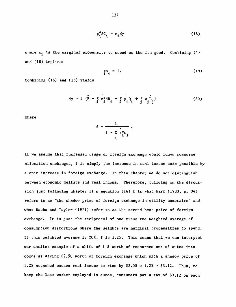
137
P dCi = midy (18)
where mi is the marginal propensity to spend on the ith good. Combining (4)
and (18) implies:
Em (19)ii
Combining (16) and (18) yields
dy = f (F- z*dRi +f PQ + E (20)Y i ii i i i i i i 20
where
f~~~~
1 - E T*mi i
i
If we assume that increased usage of foreign exchange would leave resource
allocation unchanged, f is simply the increase in real income made possible by
a unit increase in foreign exchange. In this chapter we do not distinguish
between economic welfare and real income. Therefore, building on the discus-
sion just following chapter II's equation (16) f is what Warr (1980, p. 34)
refers to as "the shadow price of foreign exchange in utility numeraire" and
what Bacha and Taylor (1971) refer to as the second best price of foreign
exchange. It is just the reciprocal of one minus the weighted average of
consumption distortions where the weights are marginal propensities to spend.
If this weighted average is 20%, f is 1.25. This means that we can interpret
our earlier example of a shift of 1 $ worth of resources out of autos into
cocoa as saving $2.50 worth of foreign exchange which with a shadow price of
1.25 attached causes real income to rise by $2.50 x 1.25 = $3.12. Thus, to
keep the last worker employed in autos, consumers pay a tax of $3.12 on each
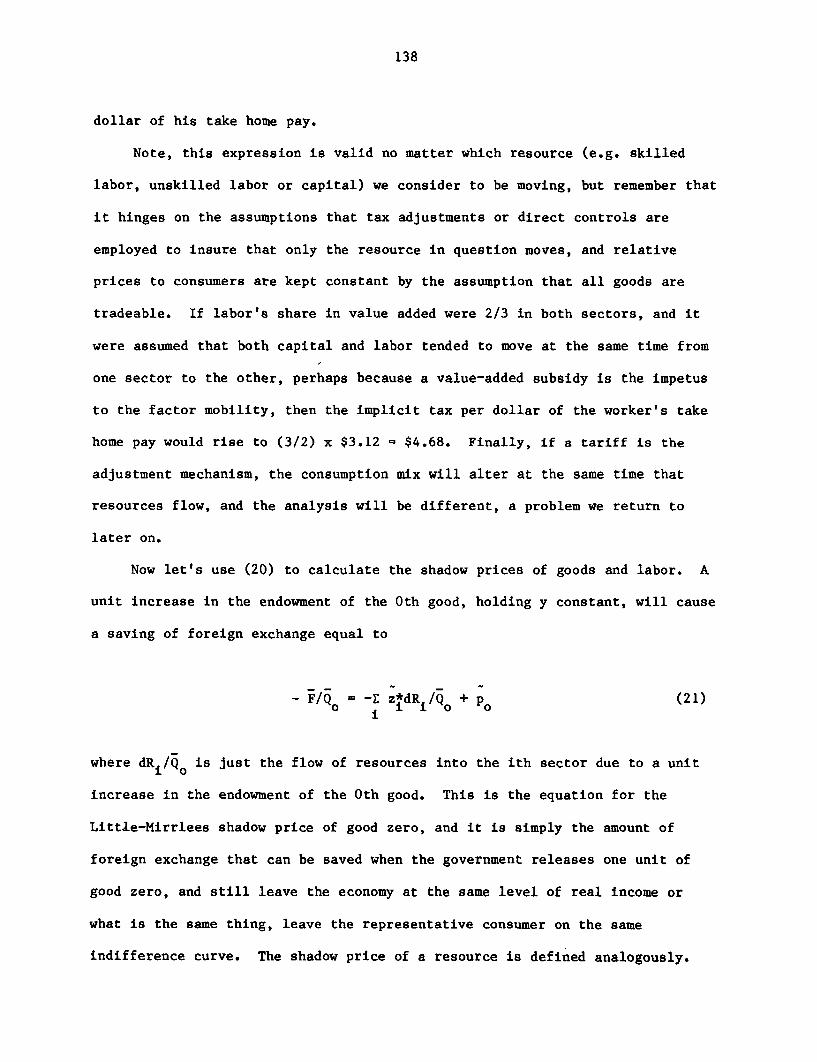
138
dollar of his take home pay.
Note, this expression is valid no matter which resource (e.g. skilled
labor, unskilled labor or capital) we consider to be moving, but remember that
it hinges on the assumptions that tax adjustments or direct controls are
employed to insure that only the resource in question moves, and relative
prices to consumers are kept constant by the assumption that all goods are
tradeable. If labor's share in value added were 2/3 in both sectors, and it
were assumed that both capital and labor tended to move at the same time from
one sector to the other, perhaps because a value-added subsidy is the impetus
to the factor mobility, then the implicit tax per dollar of the worker's take
home pay would rise to (3/2) x $3.12 = $4.68. Finally, if a tariff is the
adjustment mechanism, the consumption mix will alter at the same time that
resources flow, and the analysis will be different, a problem we return to
later on.
Now let's use (20) to calculate the shadow prices of goods and labor. A
unit increase in the endowment of the 0th good, holding y constant, will cause
a saving of foreign exchange equal to
- F/Qo =E z*dRi/Q + p (21)
where dRi/Qo is just the flow of resources into the ith sector due to a unit
increase in the endowment of the 0th good. This is the equation for the
Little-Mirrlees shadow price of good zero, and it is simply the amount of
foreign exchange that can be saved when the government releases one unit of
good zero, and still leave the economy at the same level of real income or
what is the same thing, leave the representative consumer on the same
indifference curve. The shadow price of a resource is defined analogously.
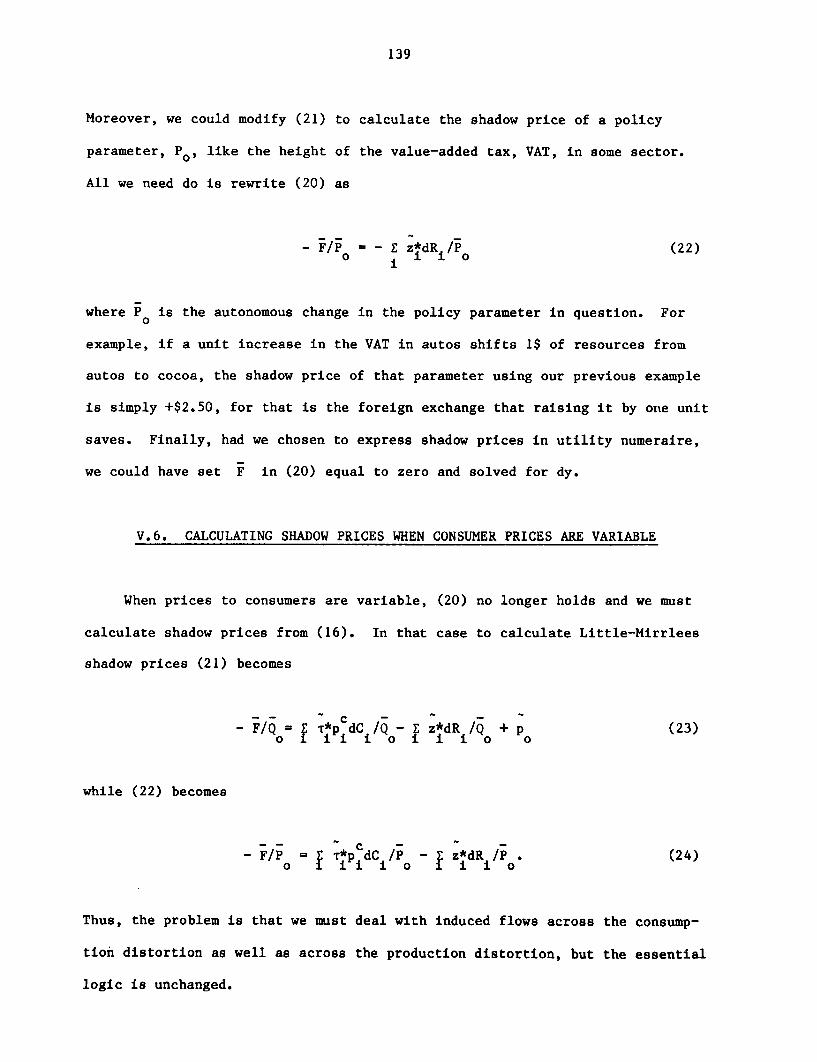
139
Moreover, we could modify (21) to calculate the shadow price of a policy
parameter, Po, like the height of the value-added tax, VAT, in some sector.
All we need do is rewrite (20) as
- F/Po E £ z*dR /P (22)i ii o
where PO is the autonomous change in the policy parameter in question. For
example, if a unit increase in the VAT in autos shifts 1$ of resources from
autos to cocoa, the shadow price of that parameter using our previous example
is simply +$2.50, for that is the foreign exchange that raising it by one unit
saves. Finally, had we chosen to express shadow prices in utility numeraire,
we could have set F in (20) equal to zero and solved for dy.
V.6. CALCULATING SHADOW PRICES WHEN CONSUMER PRICES ARE VARIABLE
When prices to consumers are variable, (20) no longer holds and we must
calculate shadow prices from (16). In that case to calculate Little-Mirrlees
shadow prices (21) becomes
- F/Qo= T*PcdC/QO E z*dR/Q + p (23)
while (22) becomes
F/Po T f PdCi/Po i z*dRi/P. (24)
Thus, the problem is that we must deal with induced flows across the consump-
tion distortion as well as across the production distortion, but the essential
logic is unchanged.
140
V.7 INSIGHTS FOR THE SHADOW PRICER
What further insights into how to shadow price goods and resources do we
get from equations (16) and (23)?
7.a Traded Goods with Fixed World Prices
First, consider a good which is traded and subject to fixed world prices.
If the government sells one unit of this good to the private sector and then
withdraws enough foreign exchange to leave private sector real income
unchanged, it is just as if the government sold the good to the foreign
sector, and as a consequence foreign exchange reserves would rise by the price
of the good, with the domestic private sector taking no part in the transac-
tion. In other words, government purchases and sales of goods of this sort,
after the private sector is compensated, leave the private sector's consump-
tion and resource allocation unchanged so that the shadow price of such a good
is simply its world price.
7.b Traded Goods with Variable World Prices
Second, now pretend that good zero is traded at a variable world price.
Suppose that the economy's resources are frozen in place, and no substitution
is permitted between goods in final demand, so that with real income fixed
consumption of each good is fixed. Then (23) tells that
/Qo Po (25)
This means that the foreign exchange saved when one unit of good zero is sold
by the government, and the private sector's real income is held constant is
141
simply the marginal revenue attached to that good when it is sold on world
markets or else the marginal expenditure attached to it when it is purchased
on world markets.
However, to the extent that domestic resources will move and consumption
patterns will alter in response to the changed world price of this good, it is
necessary to reckon with the first two terms on the right hand side of (23) in
calculating shadow prices.
7.c Non-traded Goods
Third, now pretend that good zero is a non-traded good. Also pretend
that resources are frozen and that good zero is a very good substitute in
consumption for a good that is traded with no tariff and fixed world prices
which we will call good 1, and assume neither goods 0 or 1 have excise taxes
attached. In that case (23) tells us that the shadow price of the good in
question is simply its domestic price.
Now pretend again that resources are frozen, but introduce a positive
import tariff on good 1. Government sales of good zero will lower its price
and increase its consumption, thereby lowering consumption of good 1, causing
dCl < 0 and making the first term on the right hand side of (23) negative.
This reduces the amount of foreign exchange which can be saved and still leave
the economy at its initial real income. Thus the existence of the tariff
lowers the shadow price of the non-traded good zero. The intuition behind
this is that the tariff is already artificially discouraging domestic consump-
tion of good 1, and anything which further discourages it is bad in that
regard, like the government sale of good zero.
Now let us assume that there is no substitution in consumption but that
when the government sells some of good 0, the price fall causes resources to
142
move out of the production of good 0 into the production of good 1. The
second term on the right hand side of (23) tells us that this will raise the
shadow price of good 0 above its domestic price if z* < z* for then resources1 0
will be moved out of a sector where artificial encouragements for production
are high into where they are relatively lower. This is a good thing for
economic efficiency as indicated by our criterion that demands on foreign
exchange reserves be lowered, and therefore these differential Z*s reflect
themselves in a higher shadow price for good zero.
To actually calculate shadow prices for goods and factors it is necessary
to build models which relate consumption and resource shifts to changes in
relative prices, an activity which is undertaken in Tower and Pursell (1984).
V.8 GENERALIZING THE INTERPRETATION OF THE FUNDAMENTAL EQUATION
8.a Monopoly/Monopsony Power
So far we have thought of the Tis and z*s as reflecting solely taxes andi i
subsidies, both implicit and explicit, as well as variable world prices.
Moreover we have assumed perfect competition. In fact, monopoly and monopsony
power is easy to fit into the equation. If a producer faces an upward sloping
supply of his intermediate inputs and/or a downward sloping demand for his
output, he will recognize that the marginal revenue from producing his basket
of goods is less than its price, and he will set marginal cost of production,
i.e. unit value added net of monopoly/monopsony profit equal to marginal
revenue. If we redefine vid as unit value added net of monopoly/monopsony
profit and label a as the wedge between price and marginal revenue, we can
imagine that our imperfect competitor is in fact a perfect competitor who pays
an additional value-added tax of a on disposable value added, and that this
143
tax revenue is redistributed to him as a windfall, i.e. it does not affect his
calculations. Thus, in calculating the vis throughout the economy one would
look at value added before monopoly profits, and in calculating the zis one
would include tariffs, excise taxes on intermediate inputs, explicit value
added taxes and the additional component of implicit value added taxation due
to monopoly/monopsony power.
This generalization is irrelevant with regard to tradeables that have
fixed world prices. But it is important to take into account where there are
non-traded goods. Finally, for goods with variable world prices which are
consumed or produced by a domestic monopolist/monopsonist who takes into
account the variable world price, there will be less of a distortion than
there would be if we thought of the good as being produced competitively.
8.b Minimum Wages and Taxes on Particular Factors
The fundamental equation can also be generalized to deal with taxes on
the use of particular factors.
In a simple non Harris-Todaro world a minimum wage in a particular sector
is just like a tax on hiring labor there which is redistributed to labor as a
windfall. Therefore, we can model that just like any other tax. Alterna-
tively, we can use a variant of our fundamental equation which recognizes that
if labor is pushed from a sector 1 with no minimum wage into sector 0 where
there is a minimum wage in excess of the market rate, dR0 > IdR1I, i.e. the
value of the inflow of resources into sector zero will exceed the value of
resources released by sector 1. Finally, one would deal with explicit taxes
or subsidies on factors of production in certain sectors in the same way.
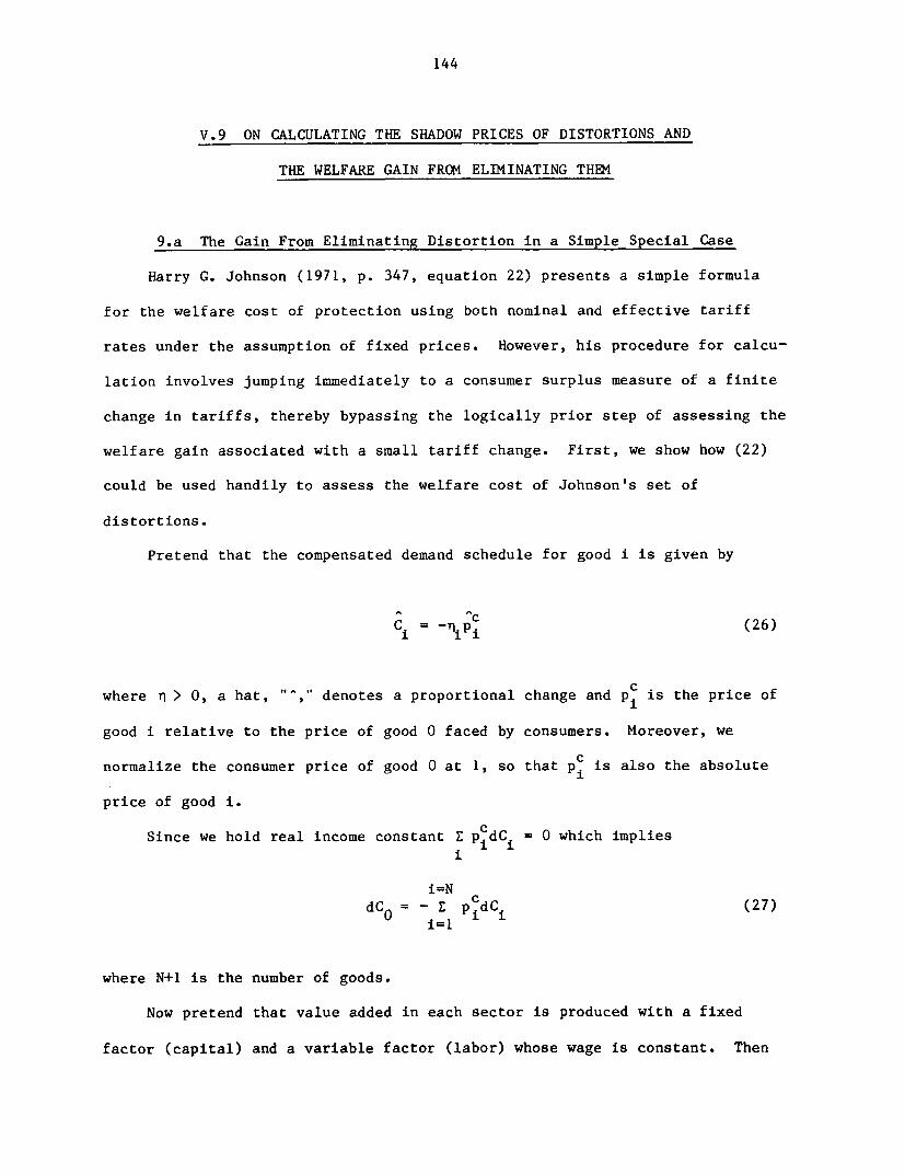
144
V.9 ON CALCULATING THE SHADOW PRICES OF DISTORTIONS AND
THE WELFARE GAIN FROM ELIMINATING THEM
9.a The Gain From Eliminating Distortion in a Simple Special Case
Harry G. Johnson (1971, p. 347, equation 22) presents a simple formula
for the welfare cost of protection using both nominal and effective tariff
rates under the assumption of fixed prices. However, his procedure for calcu-
lation involves jumping immediately to a consumer surplus measure of a finite
change in tariffs, thereby bypassing the logically prior step of assessing the
welfare gain associated with a small tariff change. First, we show how (22)
could be used handily to assess the welfare cost of Johnson's set of
distortions.
Pretend that the compensated demand schedule for good i is given by
c~~~~~~
Ci = -"iPCi (26)
where n > 0, a hat, "'," denotes a proportional change and pi is the price of
good i relative to the price of good 0 faced by consumers. Moreover, we
normalize the consumer price of good O at 1, so that p.c is also the absolute
price of good i.
Since we hold real income constant Z pcdCi = 0 which impliesi
i=NdC = z pdC (27)
where N+1 is the number of goods.
Now pretend that value added in each sector is produced with a fixed
factor (capital) and a variable factor (labor) whose wage is constant. Then
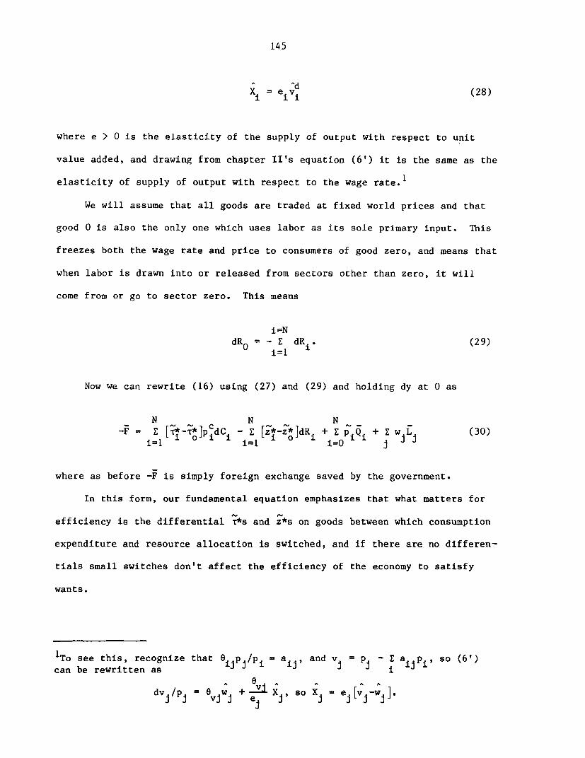
145
Ad
=i i (28)
where e > 0 is the elasticity of the supply of output with respect to unit
value added, and drawing from chapter II's equation (6') it is the same as the
elasticity of supply of output with respect to the wage rate.1
We will assume that all goods are traded at fixed world prices and that
good 0 is also the only one which uses labor as its sole primary input. This
freezes both the wage rate and price to consumers of good zero, and means that
when labor is drawn into or released from sectors other than zero, it will
come from or go to sector zero. This means
i=N
dR0 -1 dR i (29)
Now we can rewrite (16) using (27) and (29) and holding dy at 0 as
N N N-F= [;¶k-'*]pCdC, - E ~*:~]R + E P ~Qi + Ew.L (30)
1=1 o i 1=1 o i=O i i j j J
where as before -F is simply foreign exchange saved by the government.
In this form, our fundamental equation emphasizes that what matters for
efficiency is the differential T*s and z*s on goods between which consumption
expenditure and resource allocation is switched, and if there are no differen-
tials small switches don't affect the efficiency of the economy to satisfy
wants.
'To see this, recognize that 1 p /pi = a , and v = p -E a Pi so (6')can be rewritten as j J i j J i i
dvi/p J vjwj +eJ e so X = ej[vj-wJ].
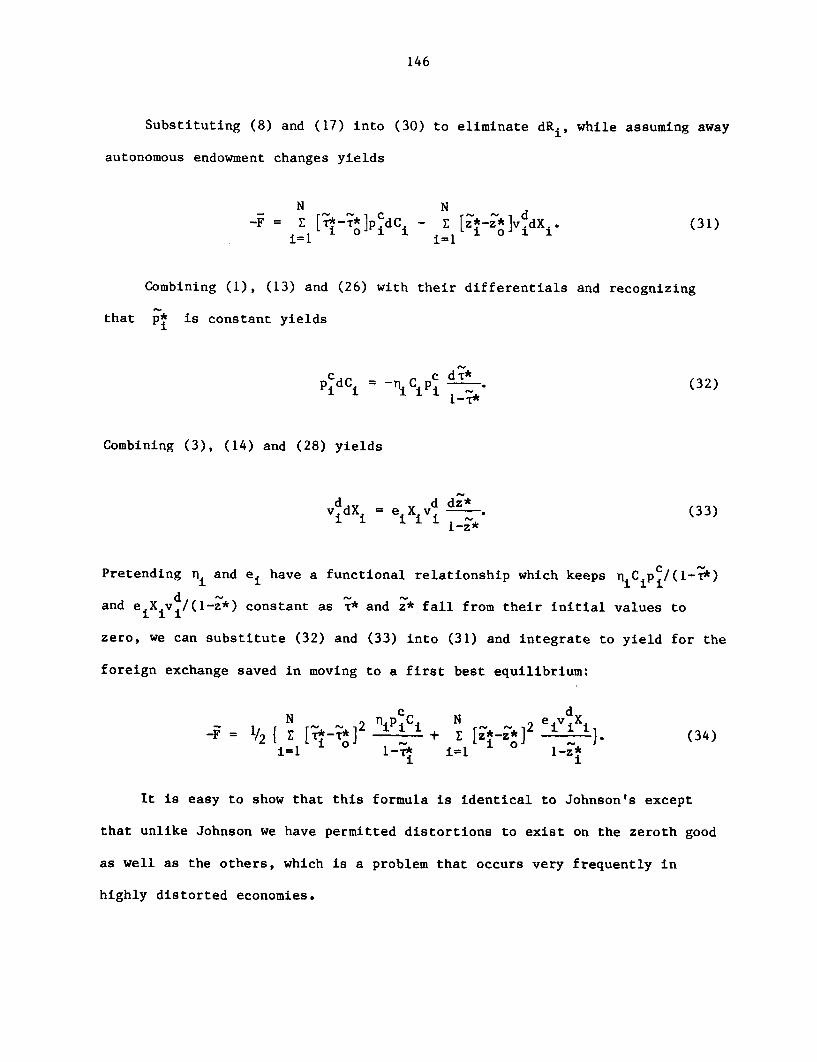
146
Substituting (8) and (17) into (30) to eliminate dRi, while assuming away
autonomous endowment changes yields
N N d4;= [;,-*] pcdC - Lz[~*ZflvidXi (31)
i-1 ioPi z[i o] idi31i=1 i=1
Combining (1), (13) and (26) with their differentials and recognizing
that p* is constant yields
pcdCi = C c dT* (32)
Combining (3), (14) and (28) yields
i i i i i (33)
Pretending ni and ei have a functional relationship which keeps nicipt/(1-;*)
d and e iXevi/(1-z*) constant as T* and z* fall from their initial values to
zero, we can substitute (32) and (33) into (31) and integrate to yield for the
foreign exchange saved in moving to a first best equilibrium:
N j2 TV i 1 N i ii (34-F = 1/2 { +
i i
It is easy to show that this formula is identical to Johnson's except
that unlike Johnson we have permitted distortions to exist on the zeroth good
as well as the others, which is a problem that occurs very frequently in
highly distorted economies.
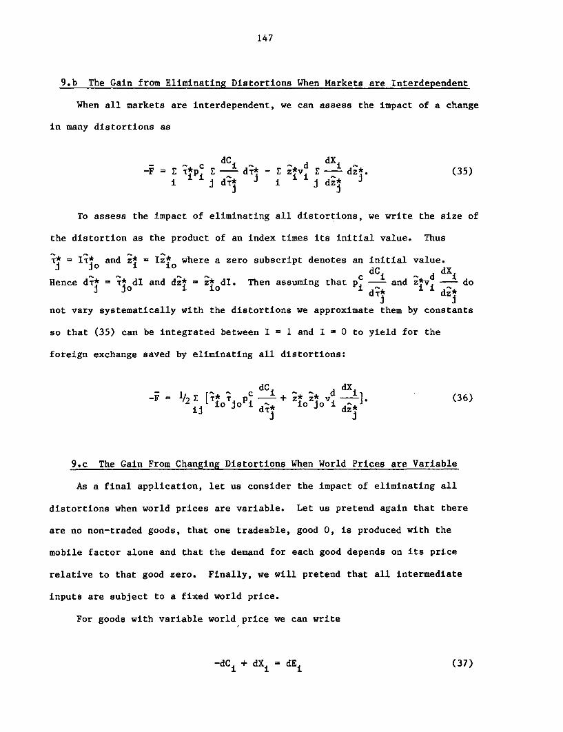
147
9.b The Gain from Eliminating Distortions When Markets are Interdependent
When all markets are interdependent, we can assess the impact of a change
in many distortions as
dCi d dX-F ~' E*PC Ec dT* - E i*vd d (35)
iii j dT* i i ii d j
To assess the impact of eliminating all distortions, we write the size of
the distortion as the product of an index times its initial value. Thus
T*= IT* and zi = Iz* where a zero subscript denotes an initial value.j Jo i io dC dX
-* -- - ~~~~c i -d iHence dT* = T* dI and dz* = z* dI. Then assuming that pi - and z*v - do
j Jo i io i i 'S
not vary systematically with the distortions we approximate them by constants
so that (35) can be integrated between I = 1 and I = 0 to yield for the
foreign exchange saved by eliminating all distortions:
dCi d dX1F/'2 I[T* c + Z * i]*(36)
~ioTp dJo 3 io Jo i dzij ° t° dT* dz* 36
9.c The Gain From Changing Distortions When World Prices are Variable
As a final application, let us consider the impact of eliminating all
distortions when world prices are variable. Let us pretend again that there
are no non-traded goods, that one tradeable, good 0, is produced with the
mobile factor alone and that the demand for each good depends on its price
relative to that good zero. Finally, we will pretend that all intermediate
inputs are subject to a fixed world price.
For goods with variable world price we can write
-dCi + dXi = dE (37)
148
where dEi is the change in exports of the good in question. Labeling ni* as
the elasticity of world excess demand for good i and substituting from (26)
and (28) we have
+ n c P + eXi V = -EinP* (38)
Since pC = (I+Ti)p*
Ac dT~ + Pi = T+T + Pt. (39)
dAlso, since vi = (1+z )v*
i i
Ad dz vi = -+i + v* (40)
and finally vi* = P*I/ (41)i vi'
Combining (38), (39), (40) and (41) yields
A dTi dzP* Ti b+Ti Zi l+Zi (42)
r i r---b zi l+z i
where
Ti ni i/Di
zi e ii i
and
eixiDi = niC + + E
i vi
along withAc dTi dz
Pi = (1 -bTi -17+T bzi l+zi43
and
d dT + [d (b e z (44)vi (bTi/dvi) Tzi vd lE+z (4
149
Then using (26), (28), (43) and (44), (31) can be written as
N dT dz-F = -E pcC*-*]n Pic [(I-b i) b
ioiii Ti d+ zi dz
(45)N dd dz- *z*] Y )bdT + [I (b Ie - }
_1[i O] Vi iI Ti/0ViI) +T + 1~(zi/ vi)] 1 i }i~~z
This is simply yet another example of how one might use the fundamental
equation.
V.10. THE GEOMETRY OF A TARIFF CUT4
The discussion in the preceding section has been algebraic, but it is
possible to explain the same ideas using geometry. Let us consider an economy
which produces and consumes two goods, an agricultural product and a
manufactured product which are both traded at fixed world prices, and suppose
elimination of the tariff on the agricultural good is contemplated. For
simplicity we choose to work with nominal tariffs and pretend that the
agricultural good is produced with one mobile and one fixed primary factor
while the manufactured good is produced with the mobile factor alone and hence
at constant costs.
Figure 3 shows the initial domestic price of the agricultural good to be
p and its final price to be equal to the world price, p*. Since S is domestic
supply and D is the compensated domestic demand curve, eliminating the
agricultural tariff contracts domestic production from SO to SF and expands
domestic consumption from Do to DF, thereby liberating domestic resources
4This section arose out of discussions with Mateen Thobani.
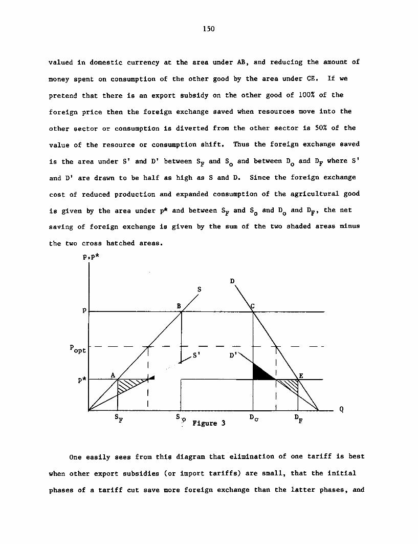
150
valued in domestic currency at the area under AB, and reducing the amount of
money spent on consumption of the other good by the area under CE. If we
pretend that there is an export subsidy on the other good of 100% of the
foreign price then the foreign exchange saved when resources move into the
other sector or consumption is diverted from the other sector is 50% of the
value of the resource or consumption shift. Thus the foreign exchange saved
is the area under S' and D' between SF and SO and between Do and DF where S'
and D' are drawn to be half as high as S and D. Since the foreign exchange
cost of reduced production and expanded consumption of the agricultural good
is given by the area under p* and between SF and SO and Do and DF, the net
saving of foreign exchange is given by the sum of the two shaded areas minus
the two cross hatched areas.
p'p*
DS
Pop F / i, 5tBC
popt S D'
A E__ _ _ _ _ _ _
p~
QSF s'9 Figure 3 Do DF
One easily sees from this diagram that elimination of one tariff is best
when other export subsidies (or import tariffs) are small, that the initial
phases of a tariff cut save more foreign exchange than the latter phases, and
151
in this case the optimum agricultural tariff is just equal to the tariff on
the other good.
To determine the gain in real income that would result from this tariff
elimination one need only multiply the foreign exchange saved by the shadow
price of foreign exchange which we have determined previously in this section.
In figure 4 we generalize this problem to reconsider the supply side of
the problem when the agricultural good uses traded intermediate inputs in
fixed proportions. v and v* are unit value added in agriculture at domestic
and international prices respectively, and v' is equal to v divided by l+ERPM
where ERPM is the effective rate of protection in the manufacturing sector,
i.e. the sector to which resources are diverted when the agricultural ERP,
ERPA, falls. The initial ERPA is ERPO so that initial unit value added in
agriculture is vo, and equilibrium is at B. When all tariffs on inputs and
outputs are eliminated the ERP falls to zero and equilibrium moves to A. The
cost in foreign exchange of reducing the gross output of the agricultural good
from X0 to XF is that quantity multiplied by v*, i.e. the area AFXOXF. This
liberates resources with a domestic currency value of ABXOXF, and given that
they find new employment in manufacturing, where the supply elasticity is
infinite they save an amount of foreign exchange equal to the area under v'
between XF and X0. Thus the net foreign exchange saving on the supply side is
the shaded area minus the cross hatched area. Clearly then, the tariff cut is
wise only if the ERP in the other sector is small. Also, it is easy to see
that welfare is maximized on the supply side when the agricultural ERP is
equal to that of the other sector, for then there is no production distortion
whatsoever.
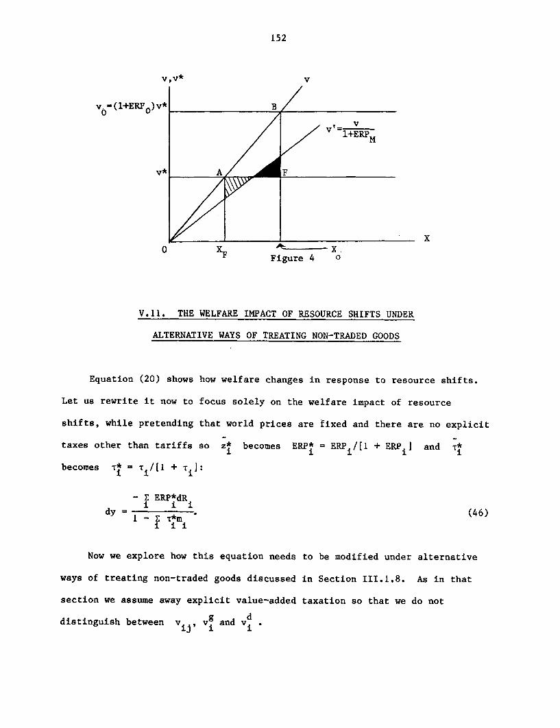
152
v,v* v
v. (1+ERP )v* B /
VI 1+ERPM
v* A F
<~~~~~~~~~~~O 0, XXF Figure 4 0
V.11. THE WELFARE IMPACT OF RESOURCE SHIFTS UNDER
ALTERNATIVE WAYS OF TREATING NON-TRADED GOODS
Equation (20) shows how welfare changes in response to resource shifts.
Let us rewrite it now to focus solely on the welfare impact of resource
shifts, while pretending that world prices are fixed and there are no explicit
taxes other than tariffs so zi becomes ERP* = ERP /[I + ERPI and T*i i i i
becomes T* = /[I + Ti]
- E ERP*dRdy = - . (46)
i ii
Now we explore how this equation needs to be modified under alternative
ways of treating non-traded goods discussed in Section III.1.8. As in that
section we assume away explicit value-added taxation so that we do not
distinguish between v Vg and v dvijI vi
153
11.a The 'Sophisticated' Corden Method
Non-traded goods cause a problem in that any resource shift will create
excess supplies and demands for non-traded goods. One way out of the problem
is the Corden method of vertically integrating the production of each good
with its non-tradeable inputs and considering factor movements between these
vertically integrated industries. In this case, the m's in (46) would be
constructed under the assumption that price changes to consumers due to
rationing or alteration of consumption taxes leave the consumption demands for
all non-tradeables constant, except in the event that the factor movement
considered is in (or out) of a non-tradeable consumer good industry, (and
perhaps other non-tradeables which feed into it) in which case such movement
would cause an excess supply (or demand) for that non-tradeable, which would
have to be matched by increased (or decreased) consumption demand for it.
11.b The Balassa Method
If the Balassa method is used for dealing with non-traded goods, we can
still use a modification of (46) to assess the welfare impact of resource
movement. When industry i expands production, primary factors must be shifted
into both industry i and the non-traded goods which feed directly and indi-
rectly into it. Assuming fixed proportions everywhere, materials balance will
be maintained when both sets of value addeds expand in the same proportions.
Thus, when resources are shifted from industry 2 to industry 1, and their
associated non-tradeables in such a way that the changed outputs of the non-
tradeables just match the changed demands for them, only a fraction X2 of the
value of them will be withdrawn from direct employment in 2 and a fraction A
will be reemployed directly in 1, with the remaining fractions (I-A )and
(1-X2) being withdrawn and replaced in intermediate non-traded goods indus-
154
tries where Ai = vi/[vi + Hi], vi is value added in i, and Hi is value added
in the non-traded goods which feed directly and indirectly into i. Thus using
(46), while remembering that in the Balassa approach we have defined the ERP
of each non-traded intermediate input to be zero gives an increase in the
economy's real income per dollar of resources transferred of
A ERP b X ERPb1 1 2 2_ ~~+b b
dy 1+ERP 1+ERP2= ~~~~~~~~~~~~~~~(47)
dR l-i miTi
where ERPb refers to a Balassa ERP. Thus while the Balassa ERPs are larger in
absolute value than the Corden ERPs, to derive expressions for the welfare
change associated with resource shift involves using the figures in different
ways, and the Balassa ERP is related to the Corden ERP, ERPC by
XERPb ERPCb . (48)
1+ERP 1+ERP
11.c The 'Crude' Corden Method
Now let us explore the implications of resource shifts when ERPs are
calculated using the 'Crude' Corden method. As this subsection is somewhat
tedious many readers will wish to skip it for our only conclusion is that by
working hard enough we can find an expression for the normative significance
of resource shifts using this measure of the ERP. From equation (IV.5) with
Vi = V , we have
V= [I + ERPc']v* (49)
where the reader will recall from the discussion just following (IV.18) that
155
we calculate value added in this method by treating non-treadeable inputs into
i just like primary factors, and ERPCC is the 'Crude' Corden ERP. Define Tji
as the amount of the jth tradeable that feeds both directly and indirectly
into producing the non-tradeables used in the production of the ith tradeable.
Then define ti s the average tariff on the Tjis which feed into i according to
E p T = (1 + t ) E p*T (50)j J Ji ii ; ii
Now recognize that the change in foreign exchange earned by allocating
increased resources to i is given by
dF = v*dX - E p*dT (51)i i j ji
where Xi is the gross output of good i.
Substituting from (49) and (50) into (51) yields
v dX E p dT
dF = i j j ji (52)cc _
1 + ERP 1 + ti i
Since labor is paid the value of its net marginal product at domestic
prices:
w dL =v dX - E p dT . (53)i i i j j ii
Let eTi be the ratio of tradeables used as intermediate inputs in good i
to value added by primary factors used both directly and indirectly in the
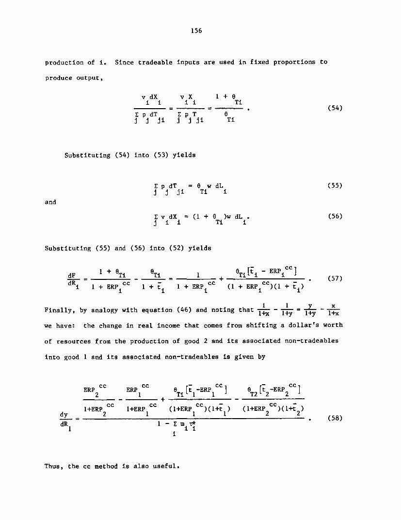
156
production of i. Since tradeable inputs are used in fixed proportions to
produce output,
v dX v X 1 + ei i i i Ti
= = . (54)E p dT E p T 8j j ii ; j ji Ti
Substituting (54) into (53) yields
E p dT =8 w dL (55)j j ji Ti i
and
E v dX =(1 + 6 )w dL. (56)j i i Ti i
Substituting (55) and (56) into (52) yields
dF 1 Ti - Ti I + Ti[ti - ERPcc]i 1 + ERPic I+ t 1 + ERPic (1 + ERP ic)(c + ti)
Finally, by analogy with equation (46) and noting that 1I - i = y x+
we have: the change in real income that comes from shifting a dollar's worth
of resources from the production of good 2 and its associated non-tradeables
into good 1 and its associated non-tradeables is given by
ERP2 cc ERPcc eTi[t-ERP CC] T2[t2-ERP 2CC]
cc cc cc ccdy 1+ERP2 1+ERPI (1+ERPI )(l+t1) (1+ERP2 )(1+t2)
dRy 1 1 1 (58)1 i i
Thus, the cc method is also useful.
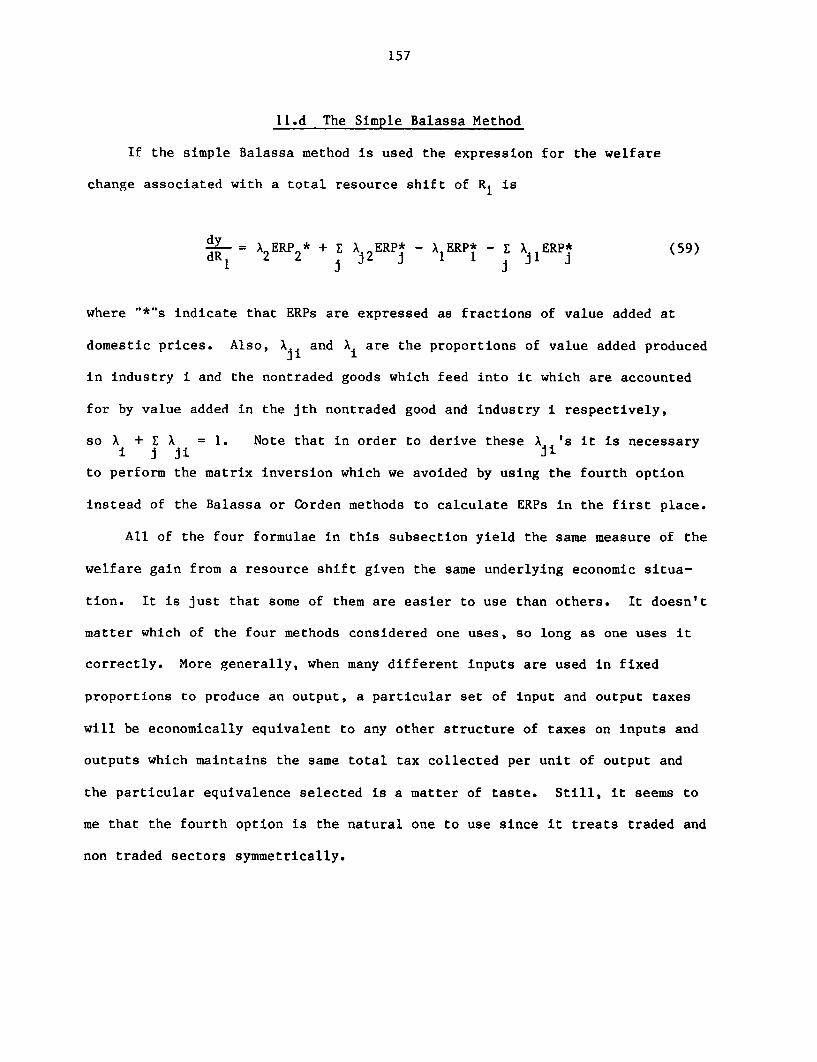
157
ll.d The Simple Balassa Method
If the simple Balassa method is used the expression for the welfare
change associated with a total resource shift of RI is
dy =X ERP * + z X. ERP* - X ERP* - E X ERP* (59)dR 2 2 . j2 j 1 1 I j i
where "*"s indicate that ERPs are expressed as fractions of value added at
domestic prices. Also, Xji and Xi are the proportions of value added produced
in industry i and the nontraded goods which feed into it which are accounted
for by value added in the jth nontraded good and industry i respectively,
so X + E X = 1. Note that in order to derive these X. 's it is necessaryi j ji ji
to perform the matrix inversion which we avoided by using the fourth option
instead of the Balassa or Corden methods to calculate ERPs in the first place.
All of the four formulae in this subsection yield the same measure of the
welfare gain from a resource shift given the same underlying economic situa-
tion. It is just that some of them are easier to use than others. It doesn't
matter which of the four methods considered one uses, so long as one uses it
correctly. More generally, when many different inputs are used in fixed
proportions to produce an output, a particular set of input and output taxes
will be economically equivalent to any other structure of taxes on inputs and
outputs which maintains the same total tax collected per unit of output and
the particular equivalence selected is a matter of taste. Still, it seems to
me that the fourth option is the natural one to use since it treats traded and
non traded sectors symmetrically.
158
V.12 IN WHAT WAY ARE NON-TRADED GOODS A PROBLEM AND HOW USEFUL
ARE STANDARD FORMULAE FOR THE EFFECTS OF TARIFF STRUCTURES?
We have shown various ways of dealing with non-traded goods and argued
that each is satisfactory, in the sense of being logically consistent. In an
important sense, however, none of them are very good. Section 9.a rederived
Harry G. Johnson's simple formula for the welfare cost of protection using
both nominal and effective tariff rates under the assumption of fixed prices.
The reason the formula is so simple is that Johnson assumes each good with a
non-zero ERP attached is produced with a sector specific factor in fixed
supply in combination with a mobile composite factor whose price is fixed. To
maintain this fixity it is necessary to assume that there are at least N
tradeables produced using mobile factors and no immobile factors where N is
the number of mobile factors in the economy. Then to make the foreign
exchange earned determinate, it is necessary to assume that all goods with
non-zero ERPs attached are produced with fixed factors in combination with
mobile factors.
This is a fairly stringent set of assumptions. But to relax it means
that it is necessary to solve the system for the impact that any adjustment in
effective or nominal tariffs would have on the prices of mobile factors, hence
outputs, consumption levels and welfare as done, for example, by Ray (1971).
Moreover, by postulating that all those goods produced with no sector specific
factors attached have zero ERPs, Johnson managed to duck the problem of unde-
fined shadow prices discussed by Bertrand (1979) and Bhagwati - Wan (1979).
If one follows Johnson's lead and postulates that there are at least N
tradeables produced using mobile factors and all the non-traded goods but no
fixed factors, where N is the number of mobile factors plus non-tradeable
159
goods in the economy, then the prices of all non-traded goods and factors of
production will be frozen, and if one further assumes that all of these goods
have zero ERPs attached, then one can treat non-traded goods plus the mobile
factors used by a sector as a composite factor, since the relative prices of
its components are fixed. In this case Johnson's formula would hold using
either the Balassa or "sophisticated" Corden methods of treating non-traded
goods, but defining e and v appropriately.
Another way to get Johnson's simple formula to apply is to assume that
each non-traded good feeds into the production of only one other good. Then
even if each non-traded good is produced with both mobile factors and a speci-
fic factor, we can integrate each non-traded good with the other good it feeds
into and treat the combination as a single good in applying Johnson's formula.
However, as soon as a single non-traded good feeds into the production of more
than one other good, this simple structure breaks down and one needs a more
complex formula than Johnson's. Moreover none of the ways of treating non-
traded goods considered in earlier sections obviates the need to solve the
system explicitly to learn the welfare impact of tariff changes when non-
traded goods are produced with specific plus mobile factors and feed into more
than one tradeable. Thus there is no simple solution to the problem of non-
traded goods or for that matter to the problem of variable world prices except
in special cases.
We should also note that it is easy for the new student of effective
protection to take Johnson's formula for the welfare cost of protection or
Balassa's (1971, p. 328 equation 26) formula for the impact of a tariff
structure on the exchange rate as the last word on the two issues. However,
Johnson's formula makes the restrictive assumptions noted above as well as
assuming that the compensated cross price elasticity of demand between all
160
goods with tariffs on them is zero, an assumption that would not be difficult
to lift as he does in the first part of his essay on the scientific tariff
(1971, pp. 198-208). Balassa's formula assumes that all goods are produced
with a fixed factor in combination with a single mobile factor and that the
domestic demand for each good depends on its price relative to the price of
the mobile factor. This too is a rather restrictive pair of assumptions.
There is no reason why one could not derive a whole slew of other quite tract-
able formulae to describe the welfare impacts of tariffs as well as their
impacts on resource allocation under alternative assumptions. Thus the
Johnson and Balassa formulae are nice straightforward passes at the problem
that yield neat tractable results, but when their problems are posed slightly
differently, different formulae will emerge. Therefore, I tend to view these
two formulae as descriptions of special cases which simply illustrate the kind
of calculus that can be fruitfully performed.
161
Chapter VI
ON THE RELATIONSHIP BETWEEN THE EFFECTIVE RATE OF
PROTECTION AND DOMESTIC RESOURCE COST*
VI.1. INTRODUCTION
The previous chapter used ERPs to calculate the welfare significance of a
resource flow from one sector to another. But as our treatment of non-traded
goods emphasized, any real world project involves a whole matrix of resource
flows between many sectors. In this chapter we show how the problem of myriad
resource flows leads naturally to using ERPs to calculate shadow prices and
hence using these shadow prices to calculate DRCs in order to evaluate
projects. Thus we see here by example how ERPs are the building blocks of
other important calculations.
Srinivasan and Bhagwati (1978, p. 107) conclude that in the presence of
distortions, the effective rate of protection is inappropriate to the task of
project selection and that the correct criterion is domestic resource cost.
Bhagwati and Srinivasan (1980) explore the problem further and come up with
two special cases in which the use of ERPs will yield the correct decision
that appropriately defined DRCs inevitably yield. They conclude that in the
absence of non-traded goods and in the presence of fixed world prices and
constant returns to scale, a project will be beneficial if and only if there
exists a critical ERP level, ERPC, such that in response to implementation of
the project no good with a higher ERP experiences an expansion in its
*This section is co-authored with Barbara L. Rollinson.
162
production, and no good with a lower ERP experiences a contraction. In this
chapter, we argue that either the DRC or the ERP is an appropriate tool for
project selection, and we generalize the Bhagwati-Srinivasan (1980) argument
to cover cases where no critical ERP separates the expanding and contracting
industries.
The only difficulty is that if one uses effective protection, one must
know and uge data on the ERPs for each of the sectors whose production is
affected by the expansion of the sector in question (call it the zeroth) as
well as the extent of resource movements in and out of these sectors. However
if one chooses instead to use the DRC route, all of the relevant information
about ERPs in sectors other than the zeroth, and resource flows elsewhere in
the economy per unit of resources attracted into the zeroth sector will be
subsumed in the shadow prices for the resources. Thus, in calculating the
DRCs for the zeroth sector, it is not necessary to look at resource flows and
ERPs elsewhere in the economy. Clearly, if many projects are to be evaluated
it is computationally more efficient to calculate shadow prices for domestic
resources, and use these to calculate DRCs, than to calculate a batch of dif-
ferentially weighted ERPs for each sector. But logically, the two approaches
are equivalent.
VI.2. ASSUMPTIONS AND DEFINITIONS
We follow Srinivasan and Bhagwati (1978), henceforth SB, in assuming all
goods are traded, which rules out any quantitative restrictions on trade; we
let output be a constant returns to scale (CRS), fixed proportions function of
intermediate inputs and a value added aggregate, where this aggregate is
itself a CRS (but not necessarily fixed proportions) function of capital and
163
labor. Also, we assume world prices are fixed and the only distortions we
permit are those assumed by SB: import tariffs, export subsidies, sticky
factor prices and factor price differentials, which may reflect themselves in
Harris-Todaro type unemployment. Finally, like SB, we assume competition
except for these factor price differentials and sticky factor prices.
We follow SB in defining DRCO as the opportunity cost of earning net
foreign exchange via increased production in sector 0 and we write it as
s sk r Q w
DRC = * (1)
0 p - p ao i io
i
where
Pi is the world price of commodity i
aio is the physical input/output coefficient showing the amount of good i used
to produce a unit of good "O", using home technology,
ko and QO are the physical input/output coefficients in sector 0 for the
primary factors, capital and labor. Thus, they are the amounts of capital and
labor used to produce an additional unit of good "O".
rs and ws are the Little-Mirrlees shadow prices of capital and labor respec-
tively, where by Little-Mirrlees shadow price of a good or factor, we mean the
amount of foreign exchange which could be withdrawn from the economy in
response to a unit increase in the economy's endowment of a good or factor and
still leave domestic utility unchanged, given all of the incentives like taxes
and tariffs in place. Defining everything in units of foreign exchange means
that the project will be found to be desirable if and only if the DRC is less
than unity.
The effective rate of protection for sector i is defined as
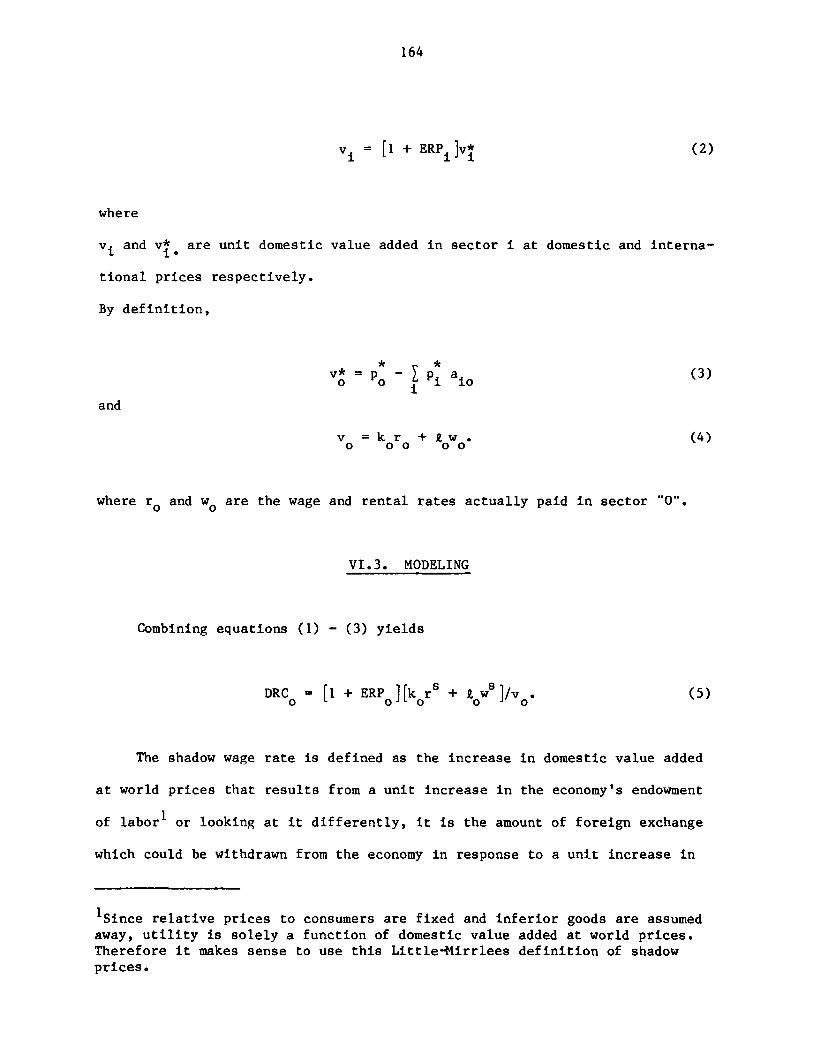
164
Vi = [1 + ERPj]v* (2)
where
Vi and v* are unit domestic value added in sector i at domestic and interna-io
tional prices respectively.
By definition,
v* = p Ip a (3)0 o iio
and
v = k0r + L wo. (4)
where ro and wo are the wage and rental rates actually paid in sector "O".
VI.3. MODELING
Combining equations (1) - (3) yields
DRCo = [1 + ERP ][k r + t w5 ]/vo. (5)0 0 0~~~
The shadow wage rate is defined as the increase in domestic value added
at world prices that results from a unit increase in the economy's endowment
of laborl or looking at it differently, it is the amount of foreign exchange
which could be withdrawn from the economy in response to a unit increase in
1Since relative prices to consumers are fixed and inferior goods are assumedaway, utility is solely a function of domestic value added at world prices.Therefore it makes sense to use this Little-Mirrlees definition of shadowprices.
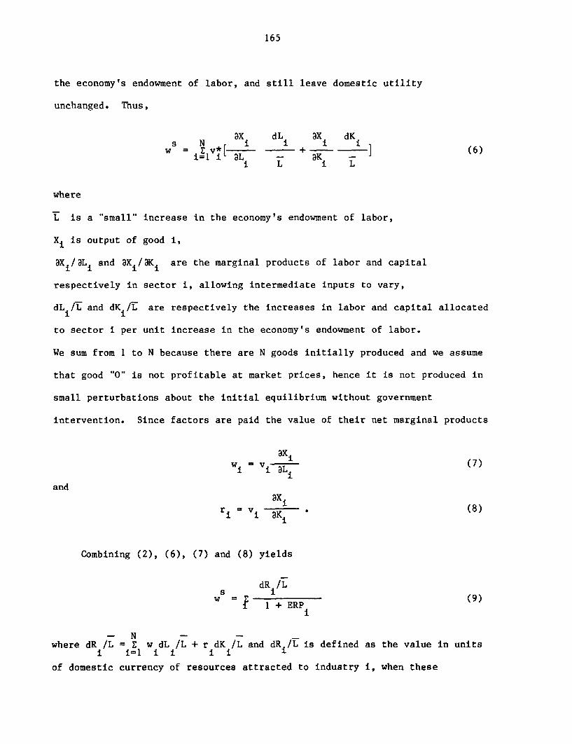
165
the economy's endowment of labor, and still leave domestic utility
unchanged. Thus,
ax dLi ax dKW = v* L K L (6)
i L i L
where
L is a "small" increase in the economy's endowment of labor,
Xiis output of good i,
axi/aLi and aXi/aKi are the marginal products of labor and capital
respectively in sector i, allowing intermediate inputs to vary,
dLi/L and dKi/L are respectively the increases in labor and capital allocated
to sector i per unit increase in the economy's endowment of labor.
We sum from 1 to N because there are N goods initially produced and we assume
that good "O" is not profitable at market prices, hence it is not produced in
small perturbations about the initial equilibrium without government
intervention. Since factors are paid the value of their net marginal products
axi
w i= v L ( 7)
andax1
ri i aKi (8 )
Combining (2), (6), (7) and (8) yields
dR /Ls i
i 1 +ERP
- N - _
where dR /L = E w dL /L + r dK /L and dR /L is defined as the value in unitsi i=1 i i i i i
of domestic currency of resources attracted to industry i, when these
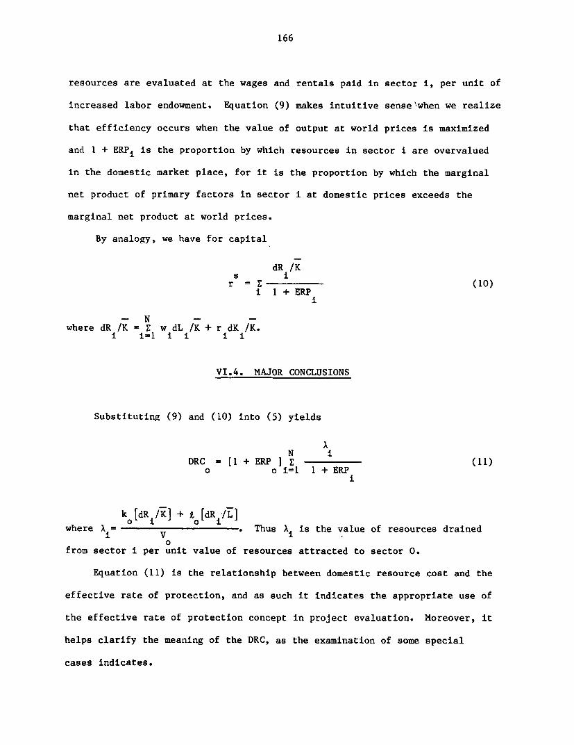
166
resources are evaluated at the wages and rentals paid in sector i, per unit of
increased labor endowment. Equation (9) makes intuitive sense when we realize
that efficiency occurs when the value of output at world prices is maximized
and 1 + ERPi is the proportion by which resources in sector i are overvalued
in the domestic market place, for it is the proportion by which the marginal
net product of primary factors in sector i at domestic prices exceeds the
marginal net product at world prices.
By analogy, we have for capital
dR /Ks ir = - (10)
i 1 + ERPi
- N _ _
where dR /K = w dL /K + r dK /K.i i=1 i i i i
VI.4. MAJOR CONCLUSIONS
Substituting (9) and (10) into (5) yields
N iDRC = [1 + ERP ] (11)
0 o i=1 1 + ERPi
ko [dRi/K] + t [dRi L ]where XA= . Thus X is the value of resources drained
i V i0
from sector i per unit value of resources attracted to sector 0.
Equation (11) is the relationship between domestic resource cost and the
effective rate of protection, and as such it indicates the appropriate use of
the effective rate of protection concept in project evaluation. Moreover, it
helps clarify the meaning of the DRC, as the examination of some special
cases indicates.
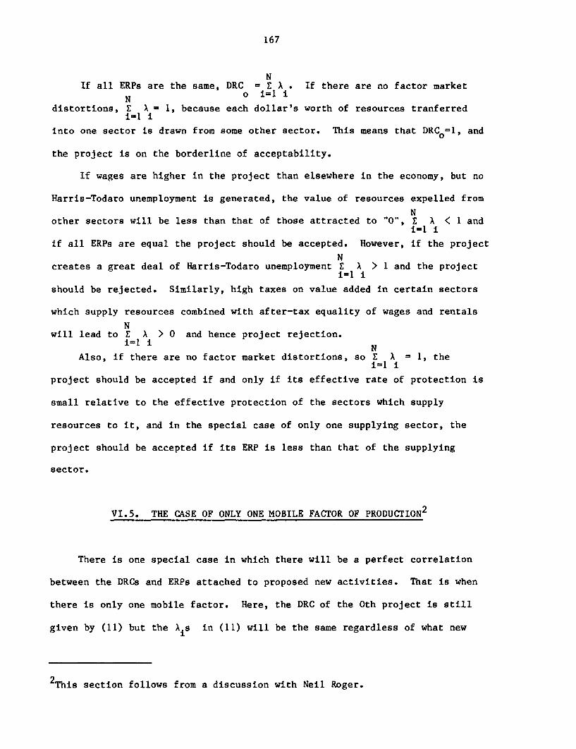
167
NIf all ERPs are the same, DRC = A . If there are no factor market
N o i=lidistortions, E X = 1, because each dollar's worth of resources tranferred
into one sector is drawn from some other sector. This means that DRC0=1, and
the project is on the borderline of acceptability.
If wages are higher in the project than elsewhere in the economy, but no
Harris-Todaro unemployment is generated, the value of resources expelled from
Nother sectors will be less than that of those attracted to O", E X < I and
i=1 i
if all ERPs are equal the project should be accepted. However, if the project
Ncreates a great deal of Harris-Todaro unemployment E X > 1 and the project
1=1 i
should be rejected. Similarly, high taxes on value added in certain sectors
which supply resources combined with after-tax equality of wages and rentals
Nwill lead to Z X > 0 and hence project rejection.
i=l i N
Also, if there are no factor market distortions, so E A - 1, the
project should be accepted if and only if its effective rate of protection is
small relative to the effective protection of the sectors which supply
resources to it, and in the special case of only one supplying sector, the
project should be accepted if its ERP is less than that of the supplying
sector.
VI.5. THE CASE OF ONLY ONE MOBILE FACTOR OF PRODUCTION2
There is one special case in which there will be a perfect correlation
between the DRCs and ERPs attached to proposed new activities. That is when
there is only one mobile factor. Here, the DRC of the 0th project is still
given by (11) but the Xis in (11) will be the same regardless of what new
2This section follows from a discussion with Neil Roger.
168
sector the labor is being drawn to.
VI.6. MORE THAN TWO FACTORS OF PRODUCTION, TWO GOODS AND
ONE TIME PERIOD
We have chosen to follow SB in postulating two mobile factors of produc-
tion but have departed from them in assuming many traded sectors instead of
just two. The reason they assumed just two sectors is so that with constant
returns to scale and only two factors of production which are mobile the
pattern of production would be determinate with no further constraints on the
system (see Bertrand (1979) and Bhagwati and Wan (1979)). Implicitly, we are
pretending that the government's incentives (perhaps progressive value added
taxes on a sector by sector basis) or else the presence of immobile factors
are sufficient to maintain the determinacy of resource allocation.
Our equation (11) relating the DRC to ERPs would be valid regardless of
the number of primary factors postulated. The only problem is that the more
factors and goods there are, the larger the matrix that one must invert in
order to obtain shadow prices.
We have also postulated a timeless model, but there is no reason we could
not have considered a project which used factors in different time periods to
produce goods in still other time periods. In that case, the DRC is calcu-
lated as before while it is recognized that discounting must be used to relate
shadow prices in one period to shadow prices in other periods.
VI.7. NON-TRADED GOODS
If there are fewer factors of production than traded goods, constant
169
returns to scale, and all factors of production are used in producing the
traded goods, the fixed world prices for traded goods will freeze the domestic
factor prices, which in turn will freeze the prices of non-traded goods. In
this circumstance, introducing non-traded goods doesn't change our analysis at
all. One could simply work with integrated industries in the 'sophisticated'
Corden fashion. Alternatively, one could work with the disaggregated indus-
tries, but define the DRC in one of two different ways.
The first alternative would be to leave the numerator as before, defined
as the amounts of primary factors evaluated at shadow prices which would be
used, while the denominator would be the increase in output minus the in-
creases in use, of the intermediate inputs used by the project, all evaluated
by their shadow prices. More generally, if this were a project which used
inputs to produce various outputs jointly, the denominator would simply be the
sum of the increases of net outputs of these various inputs and outputs, each
evaluated at its shadow price. The third alternative would be to treat the
non-traded goods just like the primary factors of production, and place them
in the numerator instead of the denominator.
Regardless of which of these three methods one used, assuming the
denominator is positive, there is a positive net social benefit associated
with the project if and only if the DRC is less than one. This is because the
numerator is the social cost associated with using up those goods and/or
factors which enter the numerator while the denominator is the social benefit
from producing the net changes in quantities of those things which enter the
denominator. Of course, shadow prices and effective protection may be
negative, and to reckon with that case, it is necessary to modify our project
selection criterion to be: select the project if and only if D - N > 0 where
D is the denominator and N is the numerator of the DRC ratio. When D > 0 this
170
boils down to the familiar DRC = N/D < 1, but when D < 0 it becomes DRC = N/D
> 1.3
Once we relax the assumption that the prices of non-traded goods are
fixed our earlier conclusions that the DRC is a weighted sum of ERPs breaks
down, because withdrawing goods and factors will cause the relative prices
faced by consumers to alter. In other words it will alter the consumption
distortion, and this must be reckoned with in calculating shadow prices.
However, even in this circumstance we can still use the DRC ratio to assess
whether or not activities which produce and/or use up non-traded goods should
be encouraged at the margin. It is only necessary that we evaluate all
factors and goods used or produced at their shadow prices, which will be
somewhat harder to calculate, and for the purpose we would need section V.2's
equation (20) which involves the flow of consumption across final demand
distortions as well as primary factors across production distortions.
VI.8. THE ACTIVITY COST-BENEFIT RATIO
This discussion boils down to the fact that the DRC has in the numerator
the social value of resources used up in order to perform an activity and in
the denominator the social value of net outputs performed by the activity.
Thus a better name for it would be the activity cost benefit ratio. The only
reason that DRC has come to be used as the term to describe the idea, is that
if all goods are traded at fixed prices their shadow prices are world prices,
so it becomes natural to identify the social value of the activity as the
foreign exchange which it earns. Similarly, in early work on the shadow
3This discussion was drawn from Pursell and Papageorgiou (1980).
171
pricing of non-traded goods and factors of production it was thought that a
reasonable shadow price for them was their domestic market price. Hence a
reasonable measure of the social cost of carrying out the activity was the
domestic currency value of the resources used in undertaking it. Thus it was
only natural to define a cost benefit ratio for a particular activity as the
value of domestic resources used to produce a unit of foreign exchange.
VI.9. HOW TO USE THE DRC
It is not possible to use the DRC for ranking industries from most desir-
able to least desirable, because it is arbitrary how one defines an activity.
Suppose that making steel requires mining coal domestically. One could either
calculate the DRC for steel or the DRC for the steel and associated coal
mining combined. The former DRC would be calculated using a shadow price for
coal which reflects its actual source of supply. Thus if marginal expansion
of the steel industry is a good thing the shadow price of steel to users will
be low and the DRC whether narrowly or broadly defined will be less than one,
but since the broadness or narrowness of an activity is a matter of defini-
tion, industries can not be ranked from most productive to least productive
using DRCs.
There is a second reason why such a ranking would not be productive. As
resources are coaxed into one sector out of others through changes in
incentives or government activities, the shadow prices of those goods and
factors which are not frozen by fixed world prices will alter, so that to
evaluate the costs and benefits of further adjustments, further DRC calcula-
tions would be needed. Thus, to conclude, except under extraordinary
circumstances DRC is a cost benefit ratio only for marginal changes, and all
172
we can say with precision is that a small expansion (contraction) of any
industry with a DRC which is less than (exceeds) unity is a good thing.
VI.10. THE DRC AND THE ADJUSTMENT MECHANISM ASSUMED
Srinivasan and Bhagwati (1978, p. 251) note that assuming the equilibrium
is unique, for existing activities, the DRCs must necessarily be unity. As
Bertrand (1979) notes, this is because if the government uses exactly the same
technology as the private sector a project consisting of expanding the output
of good i in a government firm, will have the effect of drawing all of its
resources from the private sector's production of good i, and leave the econo-
my's product mix the same as before. In terms of our mathematics, if sector
"1" were already producing, and we calculated DRCI, we would recognize that
x1= 1 with all other X's equal to zero, which clearly would give us DRC1 = 1.
This is not surprising for as SB note, Diamond and Mirrlees (1976) have
shown: for a product which is produced with constant returns to scale and
under competitive conditions,,if the government takes over some of the private
sector's production by withdrawing inputs and producing output in the same
proportions that the private sector had been previously using no levels of
outputs or inputs or prices will alter. This will leave welfare unchanged
which means that the shadow price of the output must equal the value of the
inputs at shadow prices. Another way of saying this is that the shadow value
of the resources needed to perform the activity will be equal to the shadow
value of the activity's net output, which implies that the DRC is unity.
While the logic behind this point is incontrovertable, this result is
certainly at variance with the DRC calculations as typically applied. For
example, Krueger (1966) finds that DRCs for activities performed by the
173
private sector in Turkey varied between 1.07 and 1.60. Suppose we view the
adjustment mechanism that is causing the increased output to be an increase in
the value added subsidy in that sector. Then the appropriate measure of net
benefit would be the shadow price of that subsidy multiplied by the proposed
change in the subsidy.
An alternative method, which will yield the same result is to calculate
the shadow prices of goods and factors holding the output level and input
levels in the industry constant. Then one could calculate the changes in
inputs and outputs in the industry in question which would follow from the
subsidy change. The resulting change in welfare would then be given by the
sum of the changes in net outputs multiplied by these shadow prices. More-
over, one could then define the DRC as the sum of the shadow-price weighted
changes in factor inputs divided by the sum of the shadow-price weighted
changes in net outputs of goods from the industry in question. Such an
approach I believe is what Bruno (1972), Krueger (1966; 1972) and Balassa-
Schydlowsky (1968; 1972) had in mind in their discussions of DRCs.
VI.11. IS THE DRC THE BEST COST-BENEFIT RATIO?
We have already seen that the DRC is a cost benefit ratio. Thus we can
use the DRC to estimate the welfare cost (in units of foreign exchange) of
keeping a sector alive by taking the value at shadow prices of the primary
factors devoted to it and multiply by one minus the reciprocal of its DRC.
Still, this is only an approximation, because (as noted in section 9) in most
cases shadow prices of goods and factors will change as industries expand or
contract.
Another use of DRCs, as Kemal Dervis has pointed out to me, is that they
174
indicate the percent by which efficiency in the use of primary factors would
have to grow in order to make the industry viable as an efficient use of
society's resources. Suppose we believed that by subsidizing an infant
industry we could eventually turn it into a viable producer. If its DRC were
initially 1 + a, to reduce the DRC to unity we would need to reduce our use of
primary fctors by a factor: a/(1 + a). Thus unless it were thought that this
degree of inefficiency is baby fat that an industry would automatically shed
as it grows to maturity, subsidizing it would necessarily be unwise.
However, the kind of ratio that is most likely to interest a policy maker
is the economic cost at the margin of doing something the policy maker wishes
to accomplish but to which he has trouble attaching a specific economic value,
such as increasing employment or redistributing income or fostering economic
activity in a particular region. This argues for calculating the economic
costs of achieving a unit of non-economic benefits4 through the expansion of
4A propos 'non-economic' arguments, Corden (1974, p. 155) writes "Actually the
techniques of economics can be used to analyze, or at least define more
precisely, all arguments and the use of the term 'non-economic' sometimesmeans no more than economists have not got around to analyzing an argument
properly, rather as miracles are phenomena that scientists have not yet caught
up with." In other words one should be able to take account of all 'non-
economic' benefits by appropriately defined shadow prices. The only problem
is that different observers are likely to attach different values to the same
'non-economic' result.
175
particular industries or through the use of particular economic instruments,
along the lines of the kind of linear models proposed in chapter II. Thus
the DRC is only one of many cost benefit ratios that policy makers might5
with to use.
5In fact, there are two other DRC-type measures that may prove to be useful
options. The value of primary factors used evaluated at market prices anddivided by value added at shadow prices gives the value of domestic resourcesneeded to produce a unit of foreign currency. If all goods in the calculationare traded at fixed world prices, this is simply the effective rate ofprotection coefficient. Another measure is a net DRC which would be the valueof primary factors which must be transferred to a sector to earn a unit offoreign currency net. This would be calculated as N/D with N being the marketvalue of resources needed to produce a unit of output and D being unit valueadded at shadow prices minus the shadow price of the primary factors used toproduce a unit of output. The reason that D measures net foreign exchangeearnings is that the shadow price of the primary factors indicates the oppor-tunity cost of the primary factors in their previous uses.
176
REFERENCES
Baade, R. A. and Richardson, J. D., "Commercial Policy and Functional Income
Distribution in the United States," University of Wisconsin, Department
of Economics Working Paper, No. 12 (1973).
Bacha, E. and Taylor, L., "Foreign Exchange Shadow Prices: A Critical Review
of Current Literature," Quarterly Journal of Economics 85 (May 1971):
197-224.
Balassa, B., "Tariff Protection in Industrial Countries: An Evaluation,"
Journal of Political Economy 73 (December 1965): 573-594.
Balassa, B. and Associates, The Structure of Protection in Developing
Countries, Johns Hopkins University Press, 1971.
Balassa, B. and Associates, Development Strategies in Semi-Industrial
Economies, Johns Hopkins University Press, 1982.
Balassa, B. and Schydlowsky, D. M., "Effective Tariffs, Domestic Cost of
Foreign Exchange, and the Equilibrium Exchange Rate," Journal of
Political Economy 76 (June 1968): 348-360.
Balassa, B. and Schydlowsky, D. M., "Domestic Resource Costs and Effective
Protection Once Again," Journal of Political Economy 80 (February 1972):
63-69.
Bell, C. L. G. and Zusman, P., "New Approaches to the Theory of Rental
Contracts in Agriculture," in the contributed papers section of the 17th
International Conference of Agricultural Economists, Banff, Canada,
September 1979, and published in the proceedings of the conference.
Bertrand, T. J. and Vanek, J., "The Theory of Tariffs, Taxes and Subsidies:
Some Aspects of the Second Best," American Economic Review 61 (December
1971): 925-931.
177
Bertrand, T. J., "Welfare Indexes With Interindustry Flows: Comment," Journal
of Political Economy 80 (July/August 1972): 796-800.
Bertrand, T. J., "Shadow Pricing in Distorted Economies," American Economic
Review 69 (December 1979): 902-914.
Bhagwati, J. N., "The Generalized Theory of Distortions and Welfare,"
originally published in J. N. Bhagwati, R. W. Jones, R. A. Mundell, J.
Vanek, editors, Trade, Balance of Payments and Growth: Papers in Honor
of Charles P. Kindleberger, North-Holland Publishing Company, 1971;
reprinted in Bhagwati (1981).
Bhagwati, J. N., International Trade: Selected Readings, M.I.T. Press, 1981.
Bhagwati, J. N. and Srinivasan, T. N., "The Evaluation of Projects at World
Prices Under Trade Distortions: Quantitative Restrictions, Monopoly
Power in Trade and Nontraded Goods," International Economic Review, 22
(June 1981): 385-399.
Bhagwati, J. N. and Srinivasan, T. N., "Domestic Resource Costs, Effective
Rates of Protection, and Project Analysis in Tariff-Distorted Economies,"
Quarterly Journal of Economics, 94 (February 1980): 205-209.
Bhagwati, J. N. and Srinivasan, T. N., Lectures on International Trade, M.I.T.
Press, 1983.
Bhagwati, J. N. and Wan, H., "The 'Stationarity' of Shadow Prices of Factors
in Project Evaluation With and Without Distortions," American Economic
Review 69 (June 1979): 261-273.
Bhagwati, J. N., Import Competition and Response, University of Chicago Press,
1982.
Bruno, M. "Domestic Resource Costs and Effective Protection: Clarification
and Synthesis," Journal of Political Economy 80 (February 1972): 16-33.
178
Caves, R. E. and Jones, R. W., World Trade and Payments, Little, Brown and
Company, 3rd edition, 1981.
Corden, W. M., "The Structure of a Tariff System and the Effective Protective
Rate," Journal of Political Economy 74 (June 1966): 221-237; reprinted
as chapter 9 of Bhagwati (1981).
Corden, W. M., The Theory of Protection, Clarendon Press, 1971.
Corden, W. M., Trade Policy and Economic Welfare, Oxford University Press,
1974.
Corden, W. M., "The Costs and Consequences of Protection: A Survey of
Empirical Work," pp. 51-91 of P. B. Kenen (ed.), International Trade and
Finance: Frontiers For Research, Cambridge University Press, 1975.
Corden, W. M., "The Normative Theory of International Trade," Chapter 2 of R.
W. Jones and P. B. Kenen (eds.) Handbook of International Economics, Vol.
1, North Holland Publishing Co., 1984.
Dervis, K., de Melo, J. and Robinson, S. "A General Equilibrium Analysis of
Foreign Exchange Shortages in a Developing Economy," Economic Journal 91
(December 1981): 891-906.
Dervis, K., de Melo, J. and Robinson, S., General Equilibrium Models for
Development Policy, Cambridge University Press, 1982.
Diamond, P. A. and Mirrlees, J. A. "Private Constant Returns and Public
Shadow Prices," Review of Economic Studies 43 (February 1976): 41-48.
Dixit, A. and Norman, V. Theory of International Trade, Nesbitt and Cambridge,
1982.
Dixit, A., "Tax Policy in Open Economies," in A. Auerbach and M. Feldstein
(eds.) Handbook of Public Economics, North-Holland Publishing Co.,
forthcoming.
179
Dixon, P. B., Parmenter, B. R., Sutton, J. and Vincent, D. P., Orani: A
Multisectoral Model of the Australian Economy, North-Holland Publishing
Company, 1982.
Dutton, J. and Stoeckel, A., "Effective Protection With Substitution: A
Geometric Approach," Southern Economic Journal 48 (April 1982): 909-916.
Eaton, J., Grossman, G. M., Kaempfer, W. K., and Tower, E., "The Impact of
Monopoly Pricing on the Lerner Symmetry Theorem: A Comment," Quarterly
Journal of Economics, forthcoming.
Ethier, W., "The Theory of Effective Protection in General Equilibrium:
Effective Rate Analogues of Nominal Rates," Canadian Journal of Economics
10 (May 1977): 233-245.
Evans. H. D., "The Empirical Specification of A General Equilibrium Model of
Protection in Australia," Ch. 3 of Grubel and Johnson (1971): 45-58.
Grubel, H. G. and Johnson, H. G., "Effective Tariff Protection," GATT, 1971.
Harberger, A. C., Taxation and Welfare, University of Chicago Press, 1974.
Harberger, A. C., "Economic Science and Economic Policy," typescript,
University of Chicago, undated.
Harberger, A. C., "Basic Needs Versus Distributional Weights in Social Cost
Benefit Analysis," mimeo, 1978a.
Harberger, A. C., "On The Use of Distributional Weights in Social Cost Benefit
Analysis," Journal of Political Economy, Supplement, April 1978b.
Harris, R., "Industrial Organization and The General Equilibrium Costs of
Protection in Small Open Economies," Queens University, Mimeo, March
1982.
Hartigan, J. C. and Tower, E., "Trade Policy and The American Income
Distribution," Review of Economics and Statistics 54 (May 1982): 261-
270.
180
Hartigan, J. C., "Toward A New Definition of the Effective Rate of
Protection," Weltwirtschaftliches Archiv (forthcoming).
Johansen, L., A Multi-Sectoral Study of Economic Growth, North-Holland
Publishing Co. (Ist edition 1960 and 2nd edition 1974).
Johnson, H. G., "Optimal Trade Intervention in the Presence of Domestic
Distortions," in Robert E. Baldwin et al., Trade, Growth and the Balance
of Payments: Essays in Honor of Gottfried Haberler, Rand-McNally, 1965,
3-34; reprinted as chapter 4 of Johnson (1971) and chapter 11 of Bhagwati
(1981).
Johnson, H. G., "The Cost of Protection and The Scientific Tariff," Journal of
Political Economy 68 (August 1960): 327-45; reprinted as chapter 8 of
Johnson (1971).
Johnson, H. G., "The Theory of Tariff Structure with Special Reference to
World Trade and Development," from H. G. Johnson and P. B. Kenen, Trade
and Development Libraire Droz, 1965: 9-29; reprinted as chapter 12 of
Johnson (1971).
Johnson, H. G., "The Theory of Effective Protection and Preferences,"
Economica 36 (May 1969): 119-38; reprinted as chapter 13 of Johnson
(1971).
Johnson, H. G., "'A Model of Protection and The Exchange Rate," Review of
Economic Studies, 33 (April 1966): 159-63; reprinted as chapter 14 of
Johnson (1971).
Johnson, H. G., Aspects of The Theory of Tariffs, Allen and Unwin, 1971.
Kaempfer, W. H. and Tower E., "The Balance of Payments Approach to Trade Tax
Symmetry Theorems," Weltwirtschaftliches Archiv, Band 118, (Heft 1,
1982): 148-165.
181
Kreinin, M. E., Ramsey, J. B. and Kmenta, J., "Factor Substitution and
Effective Protection Reconsidered," American Economic Review (December
1972): 891-900.
Krueger, A. O., "Some Economic Costs of Exchange Control: The Turkish Case,"
Journal of Political Economy 74 (October 1966): 466-480.
Krueger, A. O., "Evaluating Protectionist Trade Regimes: Theory and
Measurement," Journal of Political Economy 80 (February 1972): 48-62.
Little, I. M. D., Scitovsky, T. and Scott, M., Industry and Trade In Some
Developing Countries, Oxford University Press, 1970.
Little, I. M. D. and Mirrlees, J. A., Project Appraisal and Planning for
Developing Countries, Basic Books, Inc., 1974.
McKenzie, G. W., Measuring Economic Welfare: New Methods, Cambridge
University Press, 1983.
McKinnon, R. I., "Protection and the Value Added Tax," Chapter 15 of Grubel
and Johnson (1971): 287-96.
de Melo, J. A. P., "Distortions in The Factor Market: Some General Equilib-
rium Estimates," Review of Economics and Statistics, 59 (November
1977): 398-405.
de Melo, J. A. P., "Protection and Resource Allocation on a Walrasian Trade
Model," International Economic Review, 19 (February 1978a): 25-43.
de Melo, J. A. P., "Estimating the Costs of Protection: A General Equilibrium
Approach," Quarterly Journal of Economics, 92 (May 1978b): 209-26.
de Melo, J. A. P., "Tariffs and Resource Allocation in Partial and in General
Equilibrium," Weltwirtschaftliches Archiv 116 (Fasc. 1, 1980): 114-30.
de Melo, J. and Robinson, S., "Trade Policy and Resource Allocation in the
Presence of Product Differentiation," Review of Economics and Statistics
63 (May 1981): 169-77.
182
Neary, J. P., "Short Run Capital Specificity and The Pure Theory of
International Trade," Economic Journal 88 (September 1978): 488-510.
Pearson, S. R., "Net Social Profitability, Domestic Resource Costs, and
Effective Rate of Protection," Journal of Development Studies 12 (July
1976): 320-333.
Pursell, G., "Estimating Shadow Exchange Rates: The Ivory Coast," World Bank,
Mimeo, 1978.
Pursell, G. and Papageorgiou, D., "A Note on Ranking EPC-Type Incentive
Indicators," World Bank mimeo. 1980.
Ray, A., "Non-Traded Inputs and Effective Protection: A General Equilibrium
Analysis," Journal of International Economics 3 (August 1973): 245-257.
Ray, A., "Welfare Significance of Nominal and Effective Rates of Protection,"
Australian Economic Papers 19 (June 1980): 182-192.
Ruffin, R. J., "The Welfare Implications of Effective Protection," Chapter 5
of H. G. Grubel and H. G. Johnson (editors), Effective Tariff Protection,
GATT, 1971.
Sieper, E., "The Structure of General Equilibrium Shadow Pricing Rules for A
Tax Distorted Economy," Typescript, Australian National University and
Monash University, October 1980, revised January 1981.
Squire, L. and van der Tak, H. G., Economic Analysis of Projects, Johns
Hopkins University Press, 1975.
Srinivasan, T. N. and Bhagwati, J. N., "Shadow Prices for Project Selection in
the Presence of Distortions: Effective Rates of Protection and Domestic
Resource Costs," Journal of Political Economy 86 (February 1978): 97-
114; 17 of J. N. Bhagwati (1981).
Staelin, C. P., "A General Equilibrium Model of Tariffs in a Non-Competitive
Economy," Journal of International Economics 6 (February 1976): 39-64.
183
Stoeckel, A. B., A General Equilibrium Study of Mining and Agriculture in The
Australian Economy, Ph.D. Thesis, Duke University, 1978.
Taylor, L. and Black, S. L., "Practical General Equilibrium Estimation of
Resource Pulls Under Trade Liberalization," Journal of International
Economics 4 (February 1974): 37-58.
Tower, E., "On A Quick and Dirty Approach To Estimating Second Best Optimum
Tariffs," Revista Internazionale de Science Economiche E Commerciale,
31 (March 1984): 212-219.
Tower, E. and Pursell, G., "On Shadow Pricing Foreign Exchange, Goods and
Factors," World Bank, Typescript, 1984.
Warr, P., "Properties of Optimal Shadow Prices For A Tax-Distorted Open
Economy," Australian Economic Papers 19 (June 1980): 31-45.
Yabuuchi, S., "A Note on Tariff-Induced Capital Inflow and Immiseration in the
Presence of Taxation of Foreign Profits," Journal of International
Economics 12 (May 1982), 183-189.

W orld Bank Economic Analysis of Projects Economy-Wide Models andPub ications .Lyn Squire and Development PlanningfUblicAitions Herman G. van der Tak Charles R. Blitzer, Peter B. Clark,of Related Reconsiders project appraisal and rec- and Lance Taylor, editors
ommends a more systematic and con- Surveys the specification and uses ofInterest sistent estimation and application of medium-term and perspective econo-
shadow prices and a calculation of mywide planning models.rates of return that take explicit ac- Oxford University Press, 1975; 4th print-count of the project's impact on the ing, 1982. .382 pages (including selecteddistribution of income. additional readings, bibliography, subjectThe Johns Hopkins University Press, 1975; and author index).
Approaches to Purchasing 4th printing, 1981. 164 pages (including LC 4-29171. ISBN 0-19-920074-2, StockPower Parity and Real Product appendix, glossary, bibliography). No. OX 920074. $9.95 paperback.Comparisons Using Shortcuts LC 7540228. ISBN 0-8018-1818-4. Stockand Reduced Information No. IH 1818, $6.50.Sultan Ahmed French: Analyse economique des projets.Staff Working Paper No. 418. 1980. 62 Economica, 2977; 2nd printing, 1981.pages (including 14 tables, bibliography). ISBN 2-7178-0014-X, Stock No. rB 0550,Stock No. WP-0418. $3. $6.50. Financing of Investment inComparative Study of the Spanish: AnalisTs economico de proyectos. India, 1975-1985: A SourcesManagement and Organization Editorial Tecnos, 977ISBN 84-309-079- and Uses of Funds Approachof Irrigation Projects Armando Pinell-Siles and V.J.Anthony F. Bottrall Economic and Social Analysis RavishankarStaff Working Paper No. 458. 274 pages of Projects and of Price Policy: Staff Working Paper No. 543. 1982. 92(including 3 appendixes). The Morocco Fourth pages.Stock No. WP-0458. S10. Agricultural Credit Project ISBN 0-8213-0205-5. Stock No. WP 0543.
Kevin M. Cleaver S3.
NEW Staff Working Paper No. 369. 1980. 59pages (including annex tables).
Cost-Benefit Analysis: Issues Stock No. WP-0369. $3.
and MethodologyAnandarup Ray General Equilibrium ModelsExamines the numerous important NEW for Development Policycontributions to the theory and prac- Economic Evaluation of Kemal Dervis, Jaime de Melo,tice of cost-benefit analysis, consolidat- Investment Projects: and Sherman Robinsoning much of the recent work in this Provides a comprehensive study ofarea and focusing on aspects that con- Possibilities and Problems of multisector, economywide planningtinue to be controversial. Discusses al- Applying Western Methods in models with particular emphasis on is-temative types of valuation functions, China sues of trade, distribution, growth,differential weighting for income ine- Adrian Wood and structural change. Theoretical dis-quality and for disparities in the con- This paper descnbes economi t cussion of the properties of multisec-sumption of basic needs, shadow ex- bnfth aayis pae adsnbeis econoicabcost-t tor, applied general equilibriumchange rates and the valuation of benefit analysis and itsnapplicabiliwt to models is combined with numencalnontraded and traded goods and serv- ten originally as background material applications to particular countnes andicontans, v a ndat on cet of svnsadiscungt for a team of Chinese experts prepar- problems. The models considered
=rate and cor of s a s.ut ing a project appraisal manual for the range from input-output and linearratesand f shdow age ates TheChina Investmnent Bank. Other econo- programming to the more recent non-
techniques and implications of using mists, planners, and project managers linear computable general equilibriumthe more recent approaches are ex- will find it useful in doing business in (CGE) models. The authors considerplained in practical terms. Attempts to China. Concentrates on methods of es how these models can be used to ana-
the issues and polecs in cost-benefit timating shadow prices for projecf ie- lyze questions of growth and struc-analysis than is currently available in puts and outputs. Discusses project tural change, the selection of foreignthe literature. A lengthy overview is impact on the level of national income exchange regime, and the impact of al-the iterture A engty ovrvie isand the need to combine various crite- ternative development strategies onalso provided for nonspecialist read- na with the results of formal economic the distribution of income. The empiri-ers. ,,<analysis in making investmnent deci- cal applications are based both onThe Johns Hopkins University Press. 1984. sis cross-country analysis and on the ex-208 pages. perience of particular counties andLC 83-049367. ISBN 0-8018-3068-0, Stock Staff Working Paper No. 631. 1983. 53 demonstrate how such models provideNo. JH 3068, $22.50 (hardcover); ISBN 0- pages. a useful framework for policy analysis.8018-3069-9, Stock No. JH 3069, 59.50 ISBN 0-8213-0326-3. Stock No. WP 0631. Particular attention is focused on the(paperback). $3. problems of planning and policy for-
mulation in mixed-market economies No. IH 2001, $27 hardcover; ISBN 0- and to the conflicting demands of re-and on the nature of models required 8018-2006-5, Stock No. IH 2006. 59.95 gional and global estimates. Compan-to capture the important mechanisms paperback. sons are given of pnces, real per capitathat constrain policv markets. quantities, and final expenditure com-
Cambridge University Press S44 pages. The International Comparison ponents of GDP for thirty-four coun-LC 82-2307 SBN 0521-2490-0.Stock Project tries for 1975. Bv relating the results to
No lB 0556, $42.50 hardcover; ISBN 0- Three volumes that establish a world- coer tai wdely davilable national in-521-27030-8, Stock No. IB 0557, S27.95 wide system of international compan- ables, the authors develop extrapolat-paperback. sons of real product and of the pur- ing equations to estimate per capita
chasing power of currencies.igeunn oeuaeprcptThe Global Framework: An GDP for the thirty-four countnes forUpdate I , 1950 to 1978. In addition, the 1975 dis-update lAsyf iwrnDaI i tribution of world product bv regionBnan Nolan Ofs piidii and per capita income class is esti-
Staff Working Paper No. 533. 1982. 58 l mated. The 1975 results confirm rela-pages nons between both quantities and
ISBN 0-8213-0047-4. Stock No. WP 0533. pnces and per capita income found in$3. the earlier volumes.
Gnne Johns Hopkins University Press, 1982.Global Modeling in the World 398 pages.Bankt 1973-1976 LC 81-15569. ISBN 0-8018-2359-5, StockWouter Timns and Jean Waelbroeck No. IH 2359, 535 hardcover; ISBN 0-Descnbes the first stage of the global 8018-2360-9, Stock No. IH 2360, 515 pa-analvtical svstem which has become an Phase I: A System of perback.essential feature of the Bank's eco-nomic work. Evaluates the projections International Comparisons offor the world economy generated by Gross Product and Purchasing NEWthe models, of particular interest be- Powercause of the sharp rise in petroleum . Irving B. Kravis, Zoltan Kenessev, Macroeconomic andpnces in the mid-1970s. Points out Alan Heston, and Robert Summers Distributional Implications offlaws in the system which are now re-medied with new analytical tools. Establishes the methodology and pre- Sectoral Policy Interventions:
No. 54. 198. 200sents comparisons of gross domestic The Case of Energy and RiceStaff Working Paper No. 544. 1983. 200 product per capita and currencv pur- in Thailandpages. chasing power for ten countrie's in P. Amranand and W. GraisISBN 0-8213-0109-8 Stock No. WP 0544. 1970 and six of the same countres inS5. 1967 Presents an economvwide framework
for policv analvsis in rhailand. ThisHuman Factors in Project Work The Johns Hopkins Universty Press, 1975. framework-the SIAM2 model-isHeli Perrett 306 pages (ncludtng glossary, Index, used here to analyze two sets of poli-and Francis J. Lethem LC 73-19352. ISBN 0-8018-1606-8, Stock cies. Focuses on energy pricing andStaff Working Paper Vo. 397 1980 85 No. IH 1606, $27.50 hardcover. rice pricing. Shows the value of this
Staff Working Paper No. 397 2980 85 ~~~~~analytical framework for policy analy-pages (including 3 annexes, 5 charts. bzbli- Phase II: International sis that focuses on structural adjust-ography). Comparisons of Real Product ment in production and trade patterns.Stock No. WP-0397 $3. and Purchasing Power Staff Working Paper No. 627. 1984. 200
Humari Resource Development Irving B. Kravis, Alan Heston, and pages.and Economic Growth in Robert Summers Stock No. WP 627 S5.Developing Countries: A Updates Phase I and adds six new Methodologies for MeasuringSimultaneous Model countries, comparing the figures for Agricultural Price Interventionthe sixteen countries for the years 1970 AgiutrlPceIer nioDavid Wheeler and 1973. EffectsStaff Working Paper No. 407 1980. 130 The Johns Hopkins University Press. 1978. Pasquale L. Scandizzopages (including 8 appendzxes. bzbliog- 274 pages (including glossary, index). and Colin Bruceraphy). LC 77-1725Z. ISBN 0-8018-2019-7, Stock Staff Working Paper No. 394. 2980. 206
Stock No. WP-0407 55. No. iH 2019, $25 hardcover: ISBN 0- pages (including 4 appendixes, references).
Interdependence in Planning: 8018-2020-0, Stock No.JH 2020, 58.50 pa- Stock No. WP-0394. $5.Multilevel Programming perback. A Model of an AgriculturalStudies of the Ivory Coast Phase III: World Product and Household: Theory andLouis M. Goreux Income: International EvidenceProvides a system for analyzing each Comrparisons of Real GDP Howard N. Bamum and Lvncomponent of a countrv's economy in- Irving B. Kravis, Alan Heston,' Squiredependently and relates the interde- and Robert Summers Innovative model of short-run behav-
pendenres between the components. This report restates and extends the ior that combined production and con-The fohns Hopkins University Press, 19,7 methodology set out in the first two sumption decisions in a theoretically448 pages (including bibliography, index). volumes. Particular attention is given consistent fashion for an agricultural
LC 77-4793. ISBN 0-8018-20014, Stock to the problem of companng services household.
The Johns Hopkins University Press, 1980. proposes a reorientation of develop- LC 79-Z2739 ISBN 0-8018-11554, Stock218 pages (including appendix, references). ment policy to achieve more equitable No. IH 1155, 55.95 paperback.LC 78-21397. ISBN 0-8018-2225-4, Stock distribution. French: L'appreciation du risque dans.No. JH 2225, $6.95 paperback. Oxford Unzversity Press, 1974; 4th print- 1'evaluation des projets. Dunold Edzteur.
ing, 1981. 324 pages (including annex, S.5Multisector Models and the bibliography).Analysis of Alternative ISBN 0-19-920070-X, Stock No. OX Social Cost-Benefit Analysis: ADevelopment Strategies: An 920070, 59.95 paperback. Guide for Country and ProjectApplication to Korea French: Redistribution et croissance. Economists to the DerivationYuji Kubo, Jeffrey D. Lewis, Jaime Presses Universitaires de France. ISBN and Application of Economicde Melo and Sherman Robinson 22403102. S9.95. and Social Accounting PricesAn exploration of the use of multisec- Spanish: Redistribuczon con crecimiento. Colin Brucetor models as tools for analvzing the Editorial Tecnos, 1976 ISBN 84-309- Srelation between altemative develop- 0624-X. 59.95. 1taff Work1pg Paper No. c 39. Augustment strategies, growth and structural A Relationship between the 1976. 148 pages (including 6 annexes).change in a developing country. Dy- Rate of Economic Growth and Stock No. WP 0239. 55.namrc inpdut-output andC73GE mpodels the Rate, Allocation, and Techniques for Project
Korea and used as simulation laborato- Efficiency of Investment Appraisal under Uncertaintyries for analysis. Dennis Anderson Shlomo ReutlingerStaff Working Paper No. 563. 1983. 52 Discusses how the methods and re- Presents a method of evaluating risk inpages. sults of microeconomics affects the investment projects and means for us-ISBN 0-8213-0174-8. Stock No. WP 0563. analysis of growth in the relationship ing quantitative measures of risk in53 described in the title. Drawing on So- decisionmaking.
low's vintage model of growth, this The Johns Hopkins University Press, 7970;The Political Economy of paper derives an aggregate form of the 4th printing, 1979. 108 pages (includingSpecialized Farm Credit relationship and compares the ap- annex, bibliography).Institutions in Low-Income proach with those of several long- LC 74-94827. ISBN 0-8028-2154-6, StockCountries standing studies of the subject. No. IH 1154. $5.95 paperback.J.D. Von Pischke, Peter J. Staff Working Paper No. 592. 1983.44 44at is a SAM? A Layman'sHeffernan, and Dale W. Adams * g
ISBN 0-8213-0186-1. Stock No. WP 0591. Guide to Social AccountingStaff Working Paper No. 446. 1981. 102 $3. Matricespages. isinBenjamin B. KingStock No. WP-0446. S5. Risk Analysis in Project Starkin Pp no
Appraisal Staff Working Paper No. 463. 1981. e9Redistribution with Growth Louis Y. Pouliquen pages (including references).Hollis Chenery, Montek S. Discusses methodological problems Stock No. WP-0463. 53.Ahluwalia, Clive Bell, John H. and the usefulness of simulation; illus-Duloy, and Richard Jolly trated by three case studies.Descnbes existing inequality in in- The Johns Hopkins University Press, 1970;comes in developing countries and 5th printing, 1983. 90 pages.
The Developing Countries and Export Promotion PoliciesInternational Shipping Barend A. de VriesHarald Hansen Staff Working Paper No. 313. 1979. 80Staff Working Paper No. 502. 1981. 151 pages.pages (including 12 annexes, 38 tables, Stock No. WP 0313. $3.bibliography).Stock No. WP 0502. $5. NEW
Exports of Capital Goods andNEW Related Services from the
Republic of KoreaEconomics and the Politics of Larry E. Westphal, Yung W. Rhee,Protection: Some Case Studies Linsu Kim, Alice Amsden
Adjustment to External Shocks of Industries Examines Korea's spectacular exportin Developing Economies Vincent Cable growth-from $50 million of goods inBela Balassa Looks at factors which effect an indus- 1962 to $25 billion in 1982. Five kindsStaff Working Paper No. 472. 1981. 31 try's attitude toward protection by of project-related exports are character-pages (including appendix). analyzing four of Great Britain's indus- ized (overseas construction, plant ex-Stock No. WP 0472. $3. tries: footwear, knitwear, cutlery, and ports, direct investments, consulting
consumer electronics. Case studies ex- services, licensing and technical agree-Adjustment Policies and amine import competition from devel- ments). Discusses the role of these ex-
AdjustmentPolici Coun tres oping countries and adjustment op- ports in Korea's strategy for develop-Problems in Developed Countries tions exercised within each industry. ment. Shows how these strategiesMartin Wolf Study includes some explanations for conform to the country's dynamicStaff Working Paper No. 349. 1979. 236 protectionist behavior among indus- comparative advantage by enlarging itspages (including references). tries and a discussion of th,e politics of industrial base.pages No. WP 0349. $20. decisionmaking in regard to trade pol- Staff Working Paper No. 629. 1983. 80Stock No. WP 0349. $10. icy. pages.
Staff Working Paper No. 569. 1983. 80 ISBN 0-8213-0310-4.Stock No. WP 0629.Britain's Pattern of pages. $3.Specialization in Manufactured ISBN 0-8213-0199-3. Stock No. WP 0569. On Exports and EconomicGoods with Developing $3. GrowthCountries and Trade Protection Gershon FederVincent Cable and Ivonia Rebelo Effects of Non-Tariff Barriers Staff Working Paper No. 508. 1982. 24Staff Working Paper No. 425. 1980. 61 to Trade on Prices, pages (including appendix, references).pages (including 3 appendixes). Employment, and Imports: The Stock No. WP 0508. $3.Stock No. WP 0425. $3. Case of the Swedish Textile
and Clothing Industry India's ExportsCarl Hamilton Martin Wolf
NEW Staff Working Paper No. 429. 1980. 63 Despite improved performance, thepages (including appendix, bibliography). growth of India's exports continues to
Bureaucracies and the Political Stock No. WP 0429. $3. lag behind need, potential, and theEconomy of Protection: achievements of several of its competi-Reflections of a Continental Energy, International Trade, allexport perfdy examine tIhndia'sover-European and Economic Growth and 1970s, with emphasis on the cen-Patrick Messerlin Alan S. Manne and Sehun Kim tral role of incentives. The major prob-Analyzes three factors that influence Staff Working Paper No. 474. 1981. 30 lems and policies are discussed, asthe "bureaus" (bureaucrats) in their pages (including 2 appendixes, references). well as current strategic options.decisions affecting protectionism in Stock No. WP 0474. Oxford University Press. 1982. 224 pagesFrance. (including index).
Staff Working Paper No. 568. 1983. 64 LC 82-6309. ISBN 0-19-520211-2. Stockpages. No. OX 520211, $22.50 hardcover. (AISBN 0-8213-0198-5. Stock No. WP 0568. European Community specially priced edition is available in India$3. Protection against from Oxford University Press branches.)
Manufactured Imports fromCapital-Importing Oil Developing Countries: A Case Industrial Country Policy andExporters: Adjustment Issues Study in the Political Economy Adjustment to Imports fromand Policy Choices of Protection Developing CountriesAlan H. Gelb E. Verreydt and J. Waelbroeck J. M. FingerStaff Working Paper No. 475. 1981. 38 Staff Working Paper No. 432. 1980. 25 Staff Working Paper No. 470. 1981. 22pages (including 9 tables). pages. pages (including references).Stock No. WP 0475. $3. Stock No. WP 0432. $3. Stock No. WP 0470. $3.
Italian Commercial Policies in in the EEC markets but have less effect NEWthe 1970s in keeping out non-EEC imports.Enzo R. Grilli Staff Working Paper No. 567. 1983. 48 Real Wages and ExchangeStaff Working Paper No. 428. 1980. 47 ISBN 0-8213-0.97-7. Stock No. WP 0567 Rates in the Philippines, 1956-pages. $3.N 0-2309-SokN.W 57 78: An Application of theStock No. WP 0428. $3. Stolper-Samuelson-Rybczynski
Output and Employment Model of TradeChanges in a "Trade Sensitive" Deepak Lal
NEW Sector: Adjustment in the U.S. Explains the movements of real wagesFootwear Industry in the Philippines in terms of a simple
Korea's Competitive Edge: John H. Mutti and Malcolm D. regression model. Examines the coun-Managing Entry into World Bale ~~~~~~try's postwar economic performanceManaging Entry into World Bale ~~~~~~~and draws some tentative conclusions
Markets Staff Working Paper No. 430. 1980. 21 for economic policy.Yung Whee Rhee, Bruce Ross- pages (including footnotes, references). Staff Working Paper No. 604. 1983. 60Larson, and Garry Pursell Stock No. WP 0430. $3. pgs
How did Korea manage to expand its Patterns of Barriers to Trade in ISBN 0-8213-0213-2. Stock No. WP 0604.exports from less than $100 million a Sweden: A Stud in the3year in the early 1960s to more than y$20 billion a year in the early 1980s? Theory of Protection Shadow Prices for TradeTo find out about the underpinnings Lars Lundberg Strategy and Investmentof Korea's competitive edge, the au- Staff Working Paper No. 494. 1981. 35 Planning in Egyptthors asked more than 100 major Ko- pages (including 3 appendixes). John Page, Jr.rean exporters what had been impor- Stock No. WP 0494. $3. gtant for them in institutional support, Staff Working Paper No. 521. 1982. 212in technological development, and in The Political Economy of pages.marketing overseas. The findings Protection in Belgium ISBN 0-8213-0009-1. Stock No. WP 0521.show that there is a strong interaction P.K.M. Tharakan $10.between exporting and the effective-ness of a country's economic institu- Staff Working Paper No. 431. 1980. 22 Structural Change in Trade intions, both public and private. Without pages (including statistical appendix, refer- Manufactured Goods betweeneffective institutions, a country may ences). Industrial and Developingnot be able to implement effective pol- Stock No. WP 0 Countriesicies for export promotion. Conversely,successful exporting appears to give The Political Market for Bela Balassaeconomic institutions more vitality and Protection in Industrial Staff Working Paper No. 396. 1980. 46effectiveness. The findings also show Countries: Empirical Evidence pages.how Korea's selectivity-in the acqui- Kym Anderson and Robert E. Stock No. WP 0396. $3.sition of technology and in the market- Baldwining of products overseas-has been an Staff Working Paper No. 492. 1981. 28 NEWimportant part of Korea's success in pages (including references).the world marketplace. Stock No. WP 0492. $3. The Structure of Inte eationalThe Johns Hopkins University Press. June Competitiveness in the Federal1984. About 204 pages. On Protectionism in the Republic of Germany: AnISBN 0-8018-3266-7. $19.95. Netherlands Appraisal
K.A. Koekkoek, J. Kol, and L.B.M. Frank D. WeissOn the Political Economy of Mennes Probes the comparative trade advan-Protection in Germany Staff Working Paper No. 493. 1981. 70 tage of the Federal Republic of Ger-H. H. Glismann and F. D. Weiss pages (including 3 annexes, references). many in the 1980s with surprising con-Staff Working Paper No. 427. 1980. 30 Stock No. WP 0493. $3. clusions: developing countries areStages (incluing Paibliogrph) 427__1980__30 competitive with the Federal Republicpages (including bibliography). of Germany in a far wider range ofStock No. WP 0427. $3. NEW products than had been previously
Public ssistane to Inustries thought. Suggests probable trends, es-Public Assistance to Industries pecially toward developing countries.
NEW and Trade Policy in France Concludes that the faster income inBemard Bobe developing countries grows, the faster
The Political Economy of Describes the institutional structure these countries will become competi-Protection in Italy: Some through which trade police is deter- tive in an even wider range of goods.Empirical Evidence mined. Focuses on the evolution of Innovation, though a key factor, can-Enzo Grilli and Mauro La Noce France's international commerce in the not determine !-omparative advantage,1970s and assesses probable trends for because innovations spread rapidlyThis analysis is based on a model that the future. through the world economy.specifies the demand side of the mar-ket. Examines 35 industrial subsectors Staff Working Paper No. 570. 1983. 64 Staff Working Paper No. 571. 1983. 84in terms of EEC tariff protection and pages. pages.Italy's domestic subsidy assistance. ISBN 0-8213-0200-0. Stock No. WP 0570. ISBN 0-8213-0201-9. Stock No. WP 0571.Finds that tariffs protect Italian exports $3. $3.
The Structure of Protection in Trade and Employment Why the Emperor's NewDeveloping Countries Policies for Industrial Clothes Are Not Made inBela Balassa and others Development Colombia: A Case Study inThe Johns Hopkins University Press, 1971, Keith Marsden Latin American and East Asian394 pages (including 5 appendixes, index). In the last decade, the developing Manufactured ExportsLC 77-147366. ISBN 0-8018-1257-7, Stock countries have proved that they can David MorawetzNo. IH 1257. $25 hardcover. compete internationally in exporting Focuses on the exports of a particular
manufactured goods, as well as pn- commodity (clothing) from a particularmary products and services, This pa- Latin American country (Colombia) inper examines three sets of issues: (a) an attempt to understand why Latin
Testing for Direction of whether good export performance is America has been so much less suc-Exports: India's Exports of attributable to special characteristics of cessful at exporting manufacturedManufactures in the 1970s the most successful countries or goods to date than East Asia. It is the
Ashok Khanna ~~~~~~~whether their success can be readily first study to go into great detail in ex-Tessthek Khypotesi thtteeprsreplicated in other countries; (b) amining the price, and especially theTests thok hypothesis that therexportswhether the penetration of the mar- nonprice, determinants of export suc-of a developing country with an ad- kets of industrial countries has cess.vanced manufacturing sector will differ reached, or will soon reach, a limit; Oxford University Press, 1981. 208 pagesamong destinations: the capital inten- and (c) whether trade in manufactures (including appendixes, bibliography).sity of exports will be greater to the among the developing countries can(icungapdxe,blorph)more labor abundant destinations, and expand further. Concludes with a dis- LC 81-9547. ISBN 0-19-520283-X, Stockthe labor intensity of export will be cussion of the contribution of small No. OX 520283, $22 hardcover.greater to the more capital abundant enterprises to the creation of employ- Worker Adjustment todestinations. India's exports of manu- ment and the alleviation of poverty. Liberalized Trade: Costs andfactures for 1973 and 1978 are used for 1982. 70 pages (including annex). Assistance Policiesthe analysis. ISBN 0-8213-0017-2. Stock No. BK 0017. Graham Glenday, Glenn P.Staff Working Paper No. 538. 1983. 41 $5. Jenkins, and John C. Evanspages.StfWoknPaeNo42.18 7ISBN 0-8213-0132-2.Stock No. WP 0538. Staff Working Paper No. 426. 1980. 87$3. Trade in Non-Factor Services: pages (including 2 appendixes, bibliog-
Past Trends and Current Issues raphy).Andre Sapir and Emst Lutz Stock No. WP 0426. $3.Staff Working Paper No. 410. 1980. 140 World Trade and Output of
The Tokyo Round: Results and pages (including 4 annexes). Manufactures: StructuralImplications for Developing Stock No. WP 0410. $5. Trends and DevelopingCountries Countries' ExportsRia Kemper TaeiSeicsEonmcDonald B. KeesingStaff Working Paper No. 372. 1980. 38 Trade inants:and Staff Working Paper No. 316. 1979.pages (including annex). Isus74 pages (including statistical annex).pagesto inck dn No.ex) WP0Development-Related IssuesStock No WP 0316 $3
Andre Sapir and Ernst Lutz Staff Working Paper No. 480. 1981. 38 Trends in International Tradepages (including appendix, references). in Manufactured Goods and
Trade Adjustment Policies and Stock No. WP 0480. $3. Structural Change in theIncome Distribution in Three Industrial CountriesIncome Distribution in Three Bela Balassa with the assistance ofArchetype Developing Trade Policy for Developing Kenneth MeyersEconomies Countries Examines recent trends in trade in
Robmison Donald B. Keesing manufactured goods between the in-World Bank Staff Working Paper No. 353, dustrial and the developing countries.
Staff Working Paper No. 442. 1980. 91 August 1979, vii + 264 pages (including Analyzes (a) the implications of thesepages (including appendixes, references). references) trends for structural change in the in-Stock No. WP 0442. $3. Stock No WP-0353 $10 dustrial countries and (b) changes over
Stock No. WP-0353. $10. time in the current dollar value andthe commodity composition of trade in
* - . . Trade Policy Issues for the manufactured goods. RecommendsTrade among Developing Developing Countries in the teaytional trade amned at promoting in-Countries: Theory, Policy 1980s change.Issues, and Principal Trends Isaiah Frank Staff Working Paper No. 611. 1983. 44
Staff Working Paper No. 479. 1981. 116 World Bank Staff Working Paper No. 478. pages.pages (including 2 appendixes, references). August 1981. 52 pages. ISBN 0-8213-0251-5.Stock No. WP 0611.
Stock No. WP 0479. $5. Stock No. WP-0478. $3. $3.

The World Bankcm Publications Order Form
SEND TO: YOUR LOCAL DISTRIBUTOR OR TO WORLD BANK PUBLICATIONS(See the other side of this form.) P.O. BOX 37525
WASHINGTON, D.C. 20013 U.S.A.
Date
Name Ship to: (Enter if different from purchaser)
Title Name
Firm Title
Address Firm
City State_ Postal Code Address
Country TeIlephone ( ) City State_ Postal Code_
Purchaser Reference No. Country 'Telephone
Check your method of payment.Enclosed is my L Check Il International Money Order O Unesco Coupons L International Postal Coupon.Make payable to World Bank Publications for U S. dollars unless you are ordering from your local distributor.
Charge my Ol VISA L MasterCard L American Express l Choice. (Credit cards accepted only for orders addressedto World Bank Publications.)
Credit Card Account Number Expiration Date Signature
LInvoice me and please reference my Purchase Order No.
Please ship me the items listed below.
Customer InternalStock Number Author/ Title Routing Code Quantity Unit Price Total Amount s
All prices subject to change. Prices may vary by country. Allow 6-8 weeks for delivery.
Subtotal Cost $
Ibtal copies _ _ Air mail surcharge if desired ($2.00 each) $ -
Postage and handling for more than two complimentary items ($2.00 each) $
Ibtal $
IBRDO53 Thank you for your order.
Distributors of World Attn: Mr. Giancarlo Bigazzi Attn: Mr. J.M. HemandezVia Lamarmora 4 i Castello 37
Bank Publications ;0121 Madrid
ARGENTINA Florence SRI LANKA AND THE MALDIVESCarlos Hirsch, SRL, JAPAN Lake House BookshopAttn: Ms. Monica Bustos Eastern Book Service Attn: Mr. Victor WalataraFlorida 165 4° piso Attn: Mr. Terumasa Hirano 41 Wad Ramanayake MawathaGaleria Guemes 37-3, Hongo 3-Chome, Bunkyo-ku 113 Colombo 2Buenos Aires 1307 Tokyo SWEDEN
AUSTRALIA, PAPUA NEW GUINEA, KENYA ABCE Fritzes Kungl, HovbokhandelFIJI, SOLOMON ISAD,Africa Book Services (E.A.) Ltd. Attn: Mr. Eide Boxe16356ISLANDS, ~~~Attn: Mr. M.B. Dar Regerin sgatan12Bo165WESTERN SAMOA, P.O. Box03 45245ilr
VANUATU PO o 54The Australian Financial Review Nairobi SWITZERLANDInformation Service (AFRIS) KOREA, REPUBLIC OF Librairie PayotAttn: Mr. David Jamieson Pan Korea Book Corporation Attn: Mr. Henri de Perrot235-243 Jones Street Attn: Mr. Yoon-Sun Kim 6. rue GrenusBroadway P.O. Box 101, Kwanghwamun 1211 GenevaSydney, NSW 20001 Seoul TANZANIA
BELGIUM MALAYSIA Oxford Universitv PressPublications des Nations Unies University of Malaya Cooperative Attn: Mr. Anthony TheoboldAttn: Mr. Jean de Lannoy Bookshop Ltd. Maktaba Road, P.O. Box 5299av. du Roi 202 Attn: Mr. Mohammed Fahim Htj Dar es Salaam1060 Brussels Yacob THAILAND
CANADA P.O. Box 1127, Jalan Pantai Baru Central Department Store, Head OfficeLe Diffuseur Kuala Lumpur Attn: Mrs. RatanaAttn: Mrs. Suzanne Vermette MEXICO 306 Silom RoadC. P. 85, Boucherville J4B 5E6 INFOTEC BangkokQuebec Attn: Mr. Jorge Cepeda Thailand Management Association
San Lorenzo 153-I1, Col. del Valle, Attn: Mrs. SunanCOSTA RICA Deleg. Benito Juarez 308 Silom RoadLibreria Trejos mbran03100 Mexico, D.F. BangkokAttn: Mr. H ugo ChameliCalle 11-13, Av. Fernandez Guell MIDDLE EAST TUNISIASan Jose Middle East Marketing Research Soci6ti Tunisienne de DiffusionDENMARK ABureau Attn: Mr. Slaheddine Ben HamidaDENAnfnsitRatrAttn: Mr. George Vassilou 5 Avenue de CarthageSanfundslitteratur Mitsis Bld 3 5TAvnis d arhgAttn: Mr. Wilfned Roloff Miakaos l Avenue TusRosenderns Alle 11 Naaicosfia Aeu TURKEYDK-1970 Copenhagen V. Cvprus Haset Kitapevi A S.EGYPT, Arab Republic of (8ranch offices in Bahrain, Greece, Attn Mr. Izzet IzerelAl Ahram Mlorocco, Kuwait, United Arab 469, Istiklal CaddesiAl Galaa Street Emirates, Jordan) Bevoglu-IstanbulCairo NETHERLANDS UNITED KINGDOM AND
MBE BV NORTHERN IRELANDFINLAND Attn: Mr. Gerhard van Bussell Micromnfo Ltd.Akateemmnen Kirjakauppa Noorderwal 38, Attn: Mr. Roy SelwynAttn: Mr. Kari Litmanen 7241 BL Lochem Newman Lane, P.;y Box 3Keskuskatu 1, SF-00100 NORWAY Alton, Hampshire GU34 2PGHelsinki 10 Johan Grundt Tanum A.S. EnglandFRANCE Attn: Ms. Randi Mikkelborg UNITED STATESWorld Bank Publications P.O. Box 1177 Sentrum The World Bank Book Store66, avenue d'1ena Oslo 1. 60019th Street, N.W.75116 Paris PANAMA Washington, D.C. 20433GERMANY, Federal Republic of Ediciones Libreria Cultural Panamena (Postal address: P.O. Box 37525UNO-Verlag Attn: Mr. Luis Fernandez Fraguela R. Washington, D.C. 20013, U.S.A.)Attn: Mr. Joachim Krause Av. 7, Espana 16 Baker and Taylor CompanySimrockstrasse 23 Panama Zone I 501 South Gladiola AvenueD-5300 Bonn I PHILIPPINES Momence, Illinois, 60954HONG KONG, MACAU National Book Store 380 Edison WayAsia 2000 Ltd. Attn: Mrs. Socorro C. Ramos Reno, Nevada, 89564Attn: Ms. Gretchen Wearing Smith 701 Rizal Avenue 50 Kirby Avenue6 Fl., 146 Prince Edward Road Manila Somerville, New Jersey, 08876Kowloon PORTUGAL Commerce, Georgia 30599INDIA Livraria Portugal Beran AssociatesUBS Publishers' Distributors Ltd. Attn: Mr. Antonio Alves Martins 9730-E George PalerihwayAttn: Mr. D.P. Veer Ru oCro7-4Lanham, Marvland, 207615 Ansan Road. Post Box 7015 1200New Delhi 110002 Lisbon Blackwell North Amenca, Inc.(Branch offices in Bombav, Bangalore, SAUDI ARABIA 1001 Fries Mill RoadKanpur, Calcutta, and MNadras) Janr Book Store Blackwood, New Jersey 08012INDONESIA . Attn: Mr. Akram Al-Agil Sidney Kramer BooksPt. Indira Limited P 0. Box 3196 1722 H Street, N.W.Attn: Mr. Bambang Wahvudi Riyadh Washington, D.C. 20006JI, Dr. Sam Ratulangi No'. 37 SINGAPORE, TAIWAN, BURMA United Nations BookshopJakarta Pusat Information Publications Private, Ltd. United Nations Plaza
IRELAND Attn: Ms. Janet David New York, N.Y. 10017TDC Publishers 02-06 Ist Floor, Pei-Fu Industrial VENEZUELAAttn: Mr. James Booth Building LErElUEst12 North Frederick Street 24 New Industrial Road LAbreina del EsteDublin 1 Singapore Avda Francisco de Miranda. no. 52ITALY SPAIN Edificio Galipan. Aptdo. 60.337Licosa Commissionaria Sansoni SPA Mundi-Prensa Libros, S.A. Caracas 1060-A
HG 3881.5 .W57 W67 NO.664C.3
TOWER, EDWARD.
EFFECTIVE PROTECTION,DOMESTIC RESOURCE COSTS
DATE NAME AND EXTENSION NUOMBR
I
The World Bank
Headquarters European Office Tokyo Office1818 H Street, N.W. 66, avenue d'lena Kokusai BuildingWashington, D.C. 20433, U.S.A. 75116 Paris, France 1-1 Marunouchi 3-chome
Telephone: (202) 477-1234 Telephone: (1) 723-54.21 Chiyoda-ku, Tokyo 100, JapanTelex: WUI 64145 WORLDBANK Telex: 842-620628 Telephone: (03) 214-5001
RCA 248423 WORLDBK Telex: 781-26838Cable Address: INTBAFRAD
WASHINGTONDC
ISSN 0253-2115/ISBN 0-8213-0404-6


![[Eli Hinkel Sandra Fotos (Editors)] New Perspect(BookZZ.org)](https://img.pdfslide.net/doc/110x75/55cf8e47550346703b907200/eli-hinkel-sandra-fotos-editors-new-perspectbookzzorg.jpg)