Embed Size (px)
Citation preview
JOURNAL OF ALGEBRAIC STATISTICSVol. 6, No. 2, 2015, 150-167ISSN 1309-3452 – www.jalgstat.com
A linear-algebraic tool for conditional independence in-ference
Kentaro Tanaka1,∗, Milan Studeny2, Akimichi Takemura3, Tomonari Sei4
1 Faculty of Economics, Seikei University, Tokyo, Japan2 Institute of Information Theory and Automation of the CAS, Prague, Czech Republic3 Department of Mathematical Informatics, Graduate School of Information Science andTechnology, University of Tokyo, Tokyo, Japan4 Department of Mathematics, Faculty of Science and Technology, Keio University, Yoko-hama, Japan
Abstract. In this note, we propose a new linear-algebraic method for the implication problemamong conditional independence statements, which is inspired by the factorization characterizationof conditional independence. First, we give a criterion in the case of a discrete strictly positivedensity and relate it to an earlier linear-algebraic approach. Then, we extend the method to thecase of a discrete density that need not be strictly positive. Finally, we provide a computationalresult in the case of six variables.
2000 Mathematics Subject Classifications: 60A99, 68T15
Key Words and Phrases: Conditional independence inference, Automated theorem proving
1. Introduction
In this paper, we deal with the conditional independence (CI) implication problem,that is, testing whether a CI statement can be derived from a set of other CI statements.
It is well-known that there is no finite axiomatic characterization for the CI implicationproblem with general discrete probability distributions (Studeny [14]). The situation isdifferent if we restrict the class of CI statements. It is well-known that there exists a finiteaxiomatic characterization for each of the following restricted CI frames: unconditionalindependence statements (Geiger et al. [4], Matus [10]); saturated CI statements (Geigerand Pearl [5], Malvestuto [8], Malvestuto and Studeny [9]); CI statements represented byMarkov networks (Pearl and Paz [12]), and so forth. See Niepert et al. [11] and Studeny [15]for the comprehensive description.
Another way to approach the CI implication problem is based on algebra. The methodof imsets by Studeny [15] provides a powerful linear-algebraic method for testing the CI
∗Corresponding author.
Email addresses: [email protected] (Kentaro Tanaka)
http://www.jalgstat.com/ 150 c© 2015 JAlgStat All rights reserved.
Kentaro Tanaka, Milan Studeny, Akimichi Takemura, Tomonari Sei / J. Alg. Stat., 6 (2015), 150-167 151
implications. By using the method of imsets, the CI implication problem is translatedinto relations among integer-valued vectors. In Bouckaert et al. [2], a method of linearprogramming for computer testing CI implications has been proposed. In this paper, weintroduce another type of a linear-algebraic method for the CI implication problem whichis particularly suitable in the case when the distribution is strictly positive.
The structure of the paper is as follows. In Section 2, we recall the method of imsets andformulate two lemmas. In Section 3, we give a criterion applicable in the case of a discretestrictly positive density. We also give some examples there to illustrate how to use itand discuss its relation to a former linear-algebraic sufficient condition for probabilistic CIimplications. In Section 4, we deal with the case where discrete densities are not necessarilystrictly positive. In Section 5, we present a computational example to demonstrate ourmethod. Finally, in Conclusions, we summarize our results and discuss a possible relationof our approach to toric ideals.
2. Preliminaries
Throughout the paper, N is a finite indexing set for variables; to avoid the trivial casewe assume |N | ≥ 2. Given disjoint A,B ⊆ N the symbol AB will be a shorthand for theirunion A ∪B.
2.1. Distributions and conditional independence
The sample space for our (discrete multivariate) probability distributions will be thedirect product X :=
∏i∈N Xi, where Xi, i ∈ N are non-empty finite sets. Given a joint
configuration of values x ≡ [xi]i∈N ∈ X and A ⊆ N , the symbol xA will denote its marginalconfiguration [xi]i∈A. The marginal sample space for A ⊆ N will be the collection XA ofmarginal configurations for A. In particular, XN ≡ X . Observe that for A = ∅ and x ∈ Xthe marginal configuration x∅ is the empty list [xi]i∈∅. Thus, the marginal space for theempty set X∅ is also introduced: it is a one-element set containing the empty configuration.Given x ∈ XA and y ∈ XB for disjoint A,B ⊆ N , the symbol [x, y] ∈ XAB will denotetheir concatenation.
Any real-valued function on XA, for A ⊆ N , can formally be understood as a functionon X which only depends on the components in A. In this case we say it is a function ofA and denote the function as q(A; ∗), where ∗ ∈ X is the argument. Moreover, we willtake advantage of the following flexible notation: given x ∈ XD, where A ⊆ D ⊆ N , wewill write q(A;x) to denote the value of the function q (of A) for xA ∈ XA.
The density p of a probability distribution P on X is a function p : X → [0, 1] suchthat
∑x∈X p(x) = 1. It is strictly positive if p(x) > 0 for every x ∈ X . The marginal
density of p for A ⊆ N is a function on XA, usually denoted by p(A; ∗):
p(A;x) :=∑
y∈XN\A
p([xA, y]) for x ∈ X .
Kentaro Tanaka, Milan Studeny, Akimichi Takemura, Tomonari Sei / J. Alg. Stat., 6 (2015), 150-167 152
In particular, p(N ; ∗) ≡ p(∗). In our setting, conditional independence can be introducedas follows.
Definition 1. For pairwise disjoint sets A,B,C ⊆ N and the density p of a probabilitydistribution P on X , we say that A and B are conditionally independent given C withrespect to P and write A⊥⊥B | C [P ] if the following equation holds:
∀x ∈ X p(C;x) · p(ABC;x) = p(AC;x) · p(BC;x) . (1)
2.2. Factorization characterization of conditional independence
Let A,B,C ⊆ N be a triplet of pairwise disjoint sets. A well-known characterization ofA⊥⊥B | C [P ] is in terms of factorization of the marginal density p(ABC; ∗) to functionsof AC and BC. We can formally extend this characterization to the case of functions ofACD and BCD, where D denotes N \ABC. We give a straightforward proof.
Lemma 1. For a probability distribution P on X , A⊥⊥B | C [P ] is true if and only if thereexist functions q(ACD; ∗) and r(BCD; ∗) such that the marginal density decomposes asfollows:
∀x ∈ X p(ABC;x) = q(ACD;x) · r(BCD;x) . (2)
As the left-hand side of (2) only depends on the components in ABC, the right-handside of (2) does not depend on xD, despite its factors q(ACD;x) and r(BCD;x) maydepend on xD.
Proof. Assume that (1) holds and put:
q(ACD;x) =
{p(AC;x)p(C;x) if p(C;x) > 0,
0 if p(C;x) = 0,r(BCD;x) = p(BC;x) for any x ∈ X .
Note that these particular functions q(ACD;x) and r(BCD;x) do not depend of xD. Ifp(C;x) = 0, then p(ABC;x) = 0. Hence, (2) is valid. For the converse implication assumethat (2) holds. Fix some w ∈ XD and write for any x ∈ X :
p(ABC;x) = p(ABC; [xABC , w]) = q(ACD; [xAC , w]) · r(BCD; [xBC , w]),
p(AC;x) =∑y∈XB
p(ABC; [y, xAC , w]) = q(ACD; [xAC , w]) ·
∑y∈XB
r(BCD; [y, xC , w])
,
p(BC;x) =∑z∈XA
p(ABC; [z, xBC , w]) = r(BCD; [xBC , w]) ·
∑z∈XA
q(ACD; [z, xC , w])
,
p(C;x) =
∑z∈XA
q(ACD; [z, xC , w])
·∑y∈XB
r(BCD; [y, xC , w])
.
Hence, by substitution, we easily get (1), which was desired.
Kentaro Tanaka, Milan Studeny, Akimichi Takemura, Tomonari Sei / J. Alg. Stat., 6 (2015), 150-167 153
2.3. Imsets
For S ⊆ N , the symbol P(S) will denote its power set {T : T ⊆ S}. We will mainlydeal with vectors in RP(N), respectively in RK for some K ⊆ P(N). The symbol 0 willdenote the zero vector. A well-known linear basis of RP(N) consists of the identifiers δTfor sets T ⊆ N :
δT (S) =
{1 if S = T ,
0 if S 6= T .
Given L ⊆ P(N), we will denote the linear subspace of RP(N) spanned by {δT : T ∈ L} bythe symbol LL. Given u ∈ RP(N) and K ⊆ P(N), the restriction of u to the componentsin K, which is an element of RK, will be denoted by the symbol u|K. The followingobservation is evident.
Given L ⊆ P(N), u ∈ LL if and only if u|K = 0 , where K = P(N) \ L. (3)
An imset is a vector in RP(N) whose components are integers, that is, an element ofZP(N). Any conditional independence statement over N corresponds to an ordered triplet〈A,B |C〉 of pairwise disjoint sets A,B,C ⊆ N . Every such a triplet is assigned therespective semi-elementary imset u〈A,B |C〉:
u〈A,B |C〉 := δABC − δAC − δBC + δC . (4)
The triplet is trivial if either A = ∅ or B = ∅, otherwise it is called non-trivial. Observethat u〈A,B |C〉 = 0 if and only if 〈A,B |C〉 is trivial.
Definition 2. We say that u ∈ RP(N) is o-standardized if∑S⊆N
u(S) = 0 and ∀i ∈ N∑
S⊆N,i∈Su(S) = 0 .
Apparently, every semi-elementary imset u〈A,B |C〉 is o-standardized. As the set of
o-standardized vectors is a linear subspace of RP(N), linear combinations of semi-elementaryimsets are also o-standardized. Below, we employ the following auxiliary observation.
Lemma 2. Let L ⊆ P(N) be a class of sets closed under subsets, which means thatS ∈ L, T ⊆ S ⇒ T ∈ L; put K = P(N) \ L. Then an o-standardized vector u ∈ RP(N)
satisfies u|K = 0 iff, for some non-negative integer J ,
u =J∑j=1
τj · u〈Ej ,Fj |Gj〉 with real coefficients {τj}Jj=1 and EjFjGj ∈ L.
Proof. It is obvious that if u is written as the sum above then u|K = 0. We prove theconverse by induction on ` = |L ∩ {S ⊆ N : |S| ≥ 2}|. If ` = 0 then u|K = 0 meansu = 0 due to the property of o-standardization and there is no non-trivial 〈Ej , Fj |Gj〉with EjFjGj ∈ L. If ` > 0 choose inclusion maximal T ∈ L with |T | ≥ 2, find non-trivial
Kentaro Tanaka, Milan Studeny, Akimichi Takemura, Tomonari Sei / J. Alg. Stat., 6 (2015), 150-167 154
〈Ej , Fj |Gj〉 with EjFjGj = T , put τj ≡ u(T ) and apply the induction hypothesis to L\{T}and the vector u− τj · u〈Ej ,Fj |Gj〉. Note that u− τj · u〈Ej ,Fj |Gj〉 is o-standardized becauseboth u and u〈Ej ,Fj |Gj〉 are o-standardized. Moreover, the number of sets of cardinality atleast 2 in L\{T} is strictly less than `, the number of such sets in L. Thus, one can repeatthis induction step until ` decreases to 0.
3. The case of a strictly positive distribution
Let A,B,C ⊆ N , respectively Ai, Bi, Ci ⊆ N for i = 1, . . . , I, are triplets of pairwisedisjoint sets. We are dealing with the implication problem
{Ai⊥⊥Bi |Ci [P ]}Ii=1 ⇒ A⊥⊥B |C [P ], (5)
for any distribution P with a strictly positive density. The main observation is as follows.
Theorem 1. Let D denote N \ABC. If there exist real numbers {λi}Ii=1 such that
δABC +I∑i=1
λi · u〈Ai,Bi |Ci〉 ∈ LP(ACD)∪P(BCD) (6)
then the implication (5) holds for any distribution P with a strictly positive density.
Proof. By (6), there exist real numbers αS for S ∈ P(ACD) ∪ P(BCD) with
I∑i=1
λi · u〈Ai,Bi |Ci〉 = −δABC +∑
S∈P(ACD)∪P(BCD)
αS · δS . (7)
We show, for any distribution P with a strictly positive density satisfying the CI statements{Ai⊥⊥Bi |Ci [P ]}Ii=1, that
∀x ∈ X p(ABC;x) =∏
S∈P(ACD)∪P(BCD)
p(S;x)αS (8)
=∏
S∈P(ACD)
p(S;x)αS
︸ ︷︷ ︸q(ACD;x)
·∏
S∈P(BCD)\P(ACD)
p(S;x)αS
︸ ︷︷ ︸r(BCD;x)
,
which clearly implies, by Lemma 1, that A⊥⊥B |C [P ]. Since the density p of P is strictlypositive, for any fixed x ∈ X , one can write, by Ai⊥⊥Bi |Ci [P ] for i ∈ {1, . . . , I},[
∀ i 1 =p(AiBiCi;x) · p(Ci;x)
p(AiCi;x) · p(BiCi;x)
]=⇒ 1 =
I∏i=1
(p(AiBiCi;x) · p(Ci;x)
p(AiCi;x) · p(BiCi;x)
)λi.
Kentaro Tanaka, Milan Studeny, Akimichi Takemura, Tomonari Sei / J. Alg. Stat., 6 (2015), 150-167 155
The expression on the right-hand side there can be, by (7), re-written as
1 =
I∏i=1
(p(AiBiCi;x) · p(Ci;x)
p(AiCi;x) · p(BiCi;x)
)λi=
I∏i=1
∏T⊆N
p(T ;x)u〈Ai,Bi |Ci〉(T )
λi
=∏T⊆N
p(T ;x)∑I
i=1 λi·u〈Ai,Bi |Ci〉(T )(7)=
1
p(ABC;x)·
∏S∈P(ACD)∪P(BCD)
p(S;x)αS ,
and, since the term p(ABC;x) here is strictly positive, one gets (8) by multiplying it bythe factor p(ABC;x).
3.1. Equivalent formulations of the condition
In this section, we give two equivalent formulations of the sufficient condition (6) forthe implication (5) in the strictly positive case.
Lemma 3. Let A,B,C ⊆ N , respectively Ai, Bi, Ci ⊆ N for i = 1, . . . , I, be triplets ofpairwise disjoint sets; denote D ≡ N \ ABC. Given a collection of real numbers {λi}Ii=1
the following conditions are equivalent:
(a) the condition (6) holds, that is,
δABC +
I∑i=1
λi · u〈Ai,Bi |Ci〉 ∈ LP(ACD)∪P(BCD) ,
(b) for K = P(N) \ {P(ACD) ∪ P(BCD)}, one has
(u〈A,B |C〉 +I∑i=1
λi · u〈Ai,Bi |Ci〉)|K = 0 , (9)
(c) there exist real numbers {κj}Jj=1, J ≥ 0 and pairwise disjoint triplets {〈Ej , Fj |Gj〉}Jj=1
such that, for any j ∈ {1, . . . , J}, EjFjGj ∈ P(ACD) ∪ P(BCD) and
u〈A,B |C〉 +I∑i=1
λi · u〈Ai,Bi |Ci〉 +J∑j=1
κj · u〈Ej ,Fj |Gj〉 = 0 . (10)
Proof. For the proof of (a)⇔(b) consider L ≡ P(ACD) ∪ P(BCD). Since evidently−δAC−δBC+δC ∈ LL the condition in (a) means u ≡ u〈A,B |C〉+
∑Ii=1 λi ·u〈Ai,Bi |Ci〉 ∈ LL.
Thus, (a)⇔(b) follows from (3) applied to u. The equivalence (b)⇔(c) then follows fromLemma 2, where one has κj = −τj for j = 1, . . . , J .

Kentaro Tanaka, Milan Studeny, Akimichi Takemura, Tomonari Sei / J. Alg. Stat., 6 (2015), 150-167 156
3.2. Some examples
Let us discuss which of the well-known CI implications can be derived by our method.
Example 1. Consider the case |N | ≥ 3 and the CI implication, named contraction rule,
a⊥⊥ b | c, a⊥⊥ c | ∅ ⇒ a⊥⊥ bc | ∅ , (11)
where a, b, c are distinct elements of N . Since one has u〈a,bc | ∅〉− u〈a,b | c〉− u〈a,c | ∅〉 = 0 thecondition (9) is fulfilled for 〈A,B |C〉 = 〈a, bc | ∅〉, 〈A1, B1 |C1〉 = 〈a, b | c〉, 〈A2, B2 |C2〉 =〈a, c | ∅〉 and λ1 = λ2 = −1. In particular, Lemma 3 and Theorem 1 imply that contractionis valid for P with a strictly positive density. Another positive example is the so-calledweak union rule
a⊥⊥ bc | ∅ ⇒ a⊥⊥ b | c , (12)
in which case u〈a,b | c〉 − u〈a,bc | ∅〉 + u〈a,c | ∅〉 = 0 implies (10) is true for 〈A,B |C〉 = 〈a, b | c〉,〈A1, B1 |C1〉 = 〈a, bc | ∅〉, λ1 = −1, 〈E1, F1 |G1〉 = 〈a, c | ∅〉 and κ1 = +1. Thus, we haveshown the weak union holds for the distributions with a strictly positive density.
The implications from Example 1 are valid for general discrete distributions. This isnot the case in the following example.
Example 2. Consider the case |N | ≥ 3 and the following CI implication case
a⊥⊥ b | c, a⊥⊥ c | b ⇒ a⊥⊥ c | ∅ . (13)
Thus, we have 〈A,B |C〉 = 〈a, c | ∅〉, 〈A1, B1 |C1〉 = 〈a, b | c〉, 〈A2, B2 |C2〉 = 〈a, c | b〉. Toverify (9) realize that K consists of supersets of ac and observe the choice λ1 = +1 andλ2 = −1 reaches the goal. Thus, the implication (13) has been verified for any distributionwith a strictly positive density. Note that there exists a discrete distribution for which (13)does not hold; see Example 2.3 of Studeny [15]. In particular, (13) cannot be derived usingthe method discussed in Bouckaert et al. [2] applicable to general discrete distributions.
The next example shows that the repeated application of our new method makes sense.
Example 3. Consider the case |N | ≥ 3. The decomposition rule
a⊥⊥ bc | ∅ ⇒ a⊥⊥ c | ∅ , (14)
is an example of a valid CI implication, whose validity cannot be verified directly bymeans of our method. Here “directly” means that we only use our method once and donot use any other rules. In this case for 〈A,B |C〉 = 〈a, c | ∅〉, 〈A1, B1 |C1〉 = 〈a, bc | ∅〉the condition (9) is not fulfilled for any λ1 ∈ R. Indeed, assume for a contradictionthat such λ1 exists. Since abc, ac ∈ K, u〈a,bc | ∅〉(abc) = 1 and u〈a,c | ∅〉(abc) = 0 one has
0(9)= u〈a,c | ∅〉(abc)+λ1 ·u〈a,bc | ∅〉(abc) = λ1. Then, however, u〈a,c | ∅〉(ac)+λ1 ·u〈a,bc | ∅〉(ac) = 1
gives a contradiction with (9). Nevertheless, the decomposition rule (14) can be derived
Kentaro Tanaka, Milan Studeny, Akimichi Takemura, Tomonari Sei / J. Alg. Stat., 6 (2015), 150-167 157
by repeated application of (6). That is, we first derive (12) and a⊥⊥ bc | ∅ ⇒ a⊥⊥ c | b in asimilar way, and then obtain a⊥⊥ c | ∅ using the result of (13).
Next, consider the well-known intersection rule
a⊥⊥ b | c, a⊥⊥ c | b ⇒ a⊥⊥ bc | ∅ . (15)
It cannot be derived directly using our condition (6). Indeed, this time one has 〈A,B |C〉 =〈a, bc | ∅〉, 〈A1, B1 |C1〉 = 〈a, b | c〉, 〈A2, B2 |C2〉 = 〈a, c | b〉 and ab, ac, abc ∈ K. Assume fora contradiction that (u〈a,bc | ∅〉 + λ1 · u〈a,b | c〉 + λ2 · u〈a,c | b〉)|K = 0 for λ1, λ2 ∈ R. Then thefacts u〈a,bc | ∅〉(ac) = u〈a,c | b〉(ac) = 0 and u〈a,b | c〉(ac) = −1 imply λ1 = 0. Analogously,u〈a,bc | ∅〉(ab) = u〈a,b | c〉(ab) = 0 and u〈a,c | b〉(ab) = −1 implies λ2 = 0 and 1 = u〈a,bc | ∅〉(abc)gives a contradiction. Nevertheless, (15) can be derived by repeated application of (6);specifically, we first derive (13) and then obtain a⊥⊥ bc | ∅ using the result of (11).
3.3. Relation to an earlier method
A natural question is whether there is a relation of our new condition (6) to a formerimset-based sufficient condition for probabilistic CI implication proposed in § 6.2 of Stu-deny [15]. That condition was a basis of linear-algebraic methods for computer testing CIimplications applied by Bouckaert et al. [2] and can be re-phrased as follows.
Lemma 4. If there exist pairwise disjoint triplets {〈Ej , Fj |Gj〉}Jj=1 and non-negative real
numbers {ιi}Ii=1 and {κj}Jj=1, that is, ιi, κj ≥ 0 for any i, j, such that
u〈A,B |C〉 −I∑i=1
ιi · u〈Ai,Bi |Ci〉 +J∑j=1
κj · u〈Ej ,Fj |Gj〉 = 0. (16)
then the implication (5) holds for any (discrete) distribution P .
The first main difference is that (16) forces the implication (5) for any discrete prob-ability distribution P , not just for the ones with a strictly positive density. On the otherhand, the decomposition rule (14) from Example 3 shows that (16) need not imply (6).To characterize the case when (16)⇒(6) we introduce the following terminology.
Definition 3. Given disjoint A,B ⊆ N we say a triplet 〈E,F |G〉 bridges between A andB if both (EFG) ∩ A 6= ∅ and (EFG) ∩ B 6= ∅; otherwise, we say the triplet does notbridge between A and B.
Equivalently, a triplet 〈E,F |G〉 does not bridge between sets A and B if and only ifEFG ∈ P(N \B) ∪ P(N \A). A consequence of Theorem 1 and Lemma 3 is as follows.
Corollary 1. If pairwise disjoint triplets {〈Ej , Fj |Gj〉}Jj=1 not bridging between A and
B and real numbers {ιi}Ii=1 and {κj}Jj=1 exist such that (16) holds, that is,
u〈A,B |C〉 −I∑i=1
ιi · u〈Ai,Bi |Ci〉 +J∑j=1
κj · u〈Ej ,Fj |Gj〉 = 0,
Kentaro Tanaka, Milan Studeny, Akimichi Takemura, Tomonari Sei / J. Alg. Stat., 6 (2015), 150-167 158
then the condition (6) holds, implying that (5) holds for any (discrete) distribution P witha strictly positive density.
Proof. This follows from the equivalence (a)⇔(c) in Lemma 3. We put λi = −ιi fori = 1, . . . , I and observe that (16) turns into the condition (10). Then we apply Theorem 1.
Hence, the condition (16) implies our condition (6) under an additional technical as-sumption that none of the additionally considered triplets {〈Ej , Fj |Gj〉}Jj=1 bridges be-tween A and B. Note that the condition (16) in Lemma 4 requires the non-negativityof the respective coefficients while the condition in Corollary 1 does not require the non-negativity constraints. Of course, there are some cases when (6) can be applied to derive(5) for any distribution P with a strictly positive density, despite (16) with non-negativecoefficients is not applicable. From the point of view of computation, the condition (16)can be tested by linear programming tools as in Bouckaert et al. [2], while the conditions(9) and (10), which are equivalent to the condition (6), can be tested by solely checkingthe linear dependence among imsets.
3.4. Some interpretation
The observations in Lemma 4 and Corollary 1 allow one to interpret our new methodas an approach motivated by the idea of “adding extra CI statements”. Consider the im-plication problem (5) and “add” extra CI statements {Ej ⊥⊥Fj |Gj}Jj=1 to the antecedentsin (5) such that none of the added triplets bridges between A and B and obtain
{Ai⊥⊥Bi |Ci}Ii=1 ∪ {Ej ⊥⊥Fj |Gj}Jj=1 ⇒ A⊥⊥B |C . (17)
Provided we are able to verify the implication (17) by the method from Lemma 4 we canutilize the corresponding linear relation (16) in the context of Corollary 1. We may derivemore than just (17) because we have no restriction to having only non-negative coefficientshere. On the other hand, we only derive the validity of (5) for distributions with strictlypositive density.
Example 4. Consider the case |N | ≥ 4 and the following CI implication problem
a⊥⊥ b | cd, c⊥⊥ d | ab, c⊥⊥ d | a, c⊥⊥ d | b ⇒ c⊥⊥ d | ∅ , (18)
where a, b, c, d are distinct elements in N . Let us “add” some CI statements not bridgingbetween c and d, namely a⊥⊥ b | c, a⊥⊥ b | d and a⊥⊥ b | ∅ and get the implication problem
a⊥⊥ b | cd, c⊥⊥ d | ab, c⊥⊥ d | a, c⊥⊥ d | b, a⊥⊥ b | c, a⊥⊥ b | d, a⊥⊥ b | ∅ ⇒ c⊥⊥ d | ∅ .
The point is that even much stronger version of this implication can be derived by themethod from Lemma 4, namely
a⊥⊥ b | cd, c⊥⊥ d | a, c⊥⊥ d | b, a⊥⊥ b | ∅ ⇔ c⊥⊥ d | ab, a⊥⊥ b | c, a⊥⊥ b | d, c⊥⊥ d | ∅ .
In fact, this can be derived from the following linear relation of respective imsets:
u〈c,d | ∅〉 + u〈a,b | c〉 + u〈a,b | d〉 + u〈c,d | ab〉 − u〈a,b | ∅〉 − u〈c,d | a〉 − u〈c,d | b〉 − u〈a,b | cd〉 = 0 . (19)

Kentaro Tanaka, Milan Studeny, Akimichi Takemura, Tomonari Sei / J. Alg. Stat., 6 (2015), 150-167 159
To verify (18) using Corollary 1 one can re-write (19) in the form
u〈c,d | ∅〉 +[−u〈a,b | cd〉 + u〈c,d | ab〉 − u〈c,d | a〉 − u〈c,d | b〉
]+{u〈a,b | c〉 + u〈a,b | d〉 − u〈a,b | ∅〉
}= 0 ,
where the four terms in the braces correspond to {Ai⊥⊥Bi |Ci}Ii=1 and the three terms incurly brackets to {Ej ⊥⊥Fj |Gj}Jj=1.
Actually, by an analogous consideration, one can verify the validity of the implication
a⊥⊥ b | cd, c⊥⊥ d | ab, c⊥⊥ d | a, c⊥⊥ d | ∅ ⇒ c⊥⊥ d | b , (20)
for distributions with a strictly positive density. The same arguments can be used to verify
a⊥⊥ b | cd, c⊥⊥ d | a, c⊥⊥ d | b, c⊥⊥ d | ∅ ⇒ c⊥⊥ d | ab. (21)
Note that (18), (20) and (21) have been mentioned by Spohn [13] as special CI implicationsvalid for distributions with a strictly positive density. Specifically, they are gathered in theproperty (S5) from [13]. The specialty of the implication (21) is that it holds even in thecase of a general discrete distribution; see Corollary 2.1 and Example 4.1 of Studeny [15].
Remark 1. The example that (18) does not hold for general discrete distributions isvery simple: put N = {a, b, c, d}, Xi ≡ {0, 1} for i ∈ N , and define the density byassigning the value 1/2 to the configurations of values [ 0, 0, 0, 0 ], [ 1, 1, 1, 1 ] and 0 to theremaining configurations. As concerns the example that (20) does not hold in general putN = {a, b, c, d}, Xa ≡ {0, 1, 2, 3}, Xi ≡ {0, 1} for i ∈ {b, c, d} and define the density byassigning 1/4 to the configurations of values [ 0, 0, 0, 0 ], [ 1, 1, 0, 1 ], [ 2, 1, 1, 0 ], [ 3, 0, 1, 1 ]and 0 to the remaining configurations.
Remark 2. This is to warn the reader not to misinterpret our motivational remark beforeExample 4. We say there that to verify (5) we “turn” it into an extended implicationproblem (17), where none of the “added” CI statements {Ej ⊥⊥Fj |Gj}Jj=1 bridges betweenA and B. However, this extended implication problem is not equivalent to the originalone. A simple example is the following implication problem:
a⊥⊥ b | c ?⇒ a⊥⊥ b | ∅ .
This is not a valid CI implication even for distributions with a strictly positive densitydespite the extended implication problem
a⊥⊥ b | c, a⊥⊥ c | ∅ ⇒ a⊥⊥ b | ∅
is a valid CI implication. The crucial argument to verify (5) is the linear relation (16) andthe fact that the only bridging triplets between A and B in (5) are of the form 〈Ai, Bi |Ci〉.
Kentaro Tanaka, Milan Studeny, Akimichi Takemura, Tomonari Sei / J. Alg. Stat., 6 (2015), 150-167 160
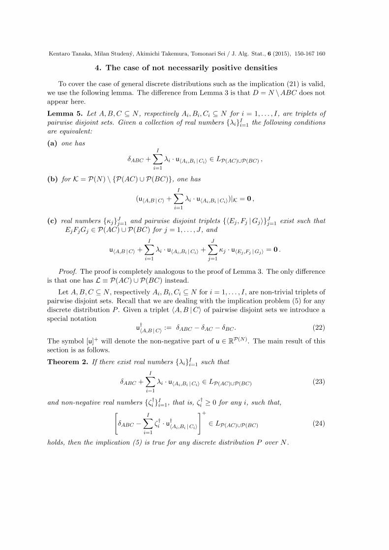
4. The case of not necessarily positive densities
To cover the case of general discrete distributions such as the implication (21) is valid,we use the following lemma. The difference from Lemma 3 is that D = N \ABC does notappear here.
Lemma 5. Let A,B,C ⊆ N , respectively Ai, Bi, Ci ⊆ N for i = 1, . . . , I, are triplets ofpairwise disjoint sets. Given a collection of real numbers {λi}Ii=1 the following conditionsare equivalent:
(a) one has
δABC +I∑i=1
λi · u〈Ai,Bi |Ci〉 ∈ LP(AC)∪P(BC) ,
(b) for K = P(N) \ {P(AC) ∪ P(BC)}, one has
(u〈A,B |C〉 +I∑i=1
λi · u〈Ai,Bi |Ci〉)|K = 0 ,
(c) real numbers {κj}Jj=1 and pairwise disjoint triplets {〈Ej , Fj |Gj〉}Jj=1 exist such thatEjFjGj ∈ P(AC) ∪ P(BC) for j = 1, . . . , J , and
u〈A,B |C〉 +
I∑i=1
λi · u〈Ai,Bi |Ci〉 +
J∑j=1
κj · u〈Ej ,Fj |Gj〉 = 0 .
Proof. The proof is completely analogous to the proof of Lemma 3. The only differenceis that one has L ≡ P(AC) ∪ P(BC) instead.
Let A,B,C ⊆ N , respectively Ai, Bi, Ci ⊆ N for i = 1, . . . , I, are non-trivial triplets ofpairwise disjoint sets. Recall that we are dealing with the implication problem (5) for anydiscrete distribution P . Given a triplet 〈A,B |C〉 of pairwise disjoint sets we introduce aspecial notation
u†〈A,B |C〉 := δABC − δAC − δBC . (22)
The symbol [u]+ will denote the non-negative part of u ∈ RP(N). The main result of thissection is as follows.
Theorem 2. If there exist real numbers {λi}Ii=1 such that
δABC +I∑i=1
λi · u〈Ai,Bi |Ci〉 ∈ LP(AC)∪P(BC) (23)
and non-negative real numbers {ζ†i }Ii=1, that is, ζ†i ≥ 0 for any i, such that,[δABC −
I∑i=1
ζ†i · u†〈Ai,Bi |Ci〉
]+∈ LP(AC)∪P(BC) (24)
holds, then the implication (5) is true for any discrete distribution P over N .
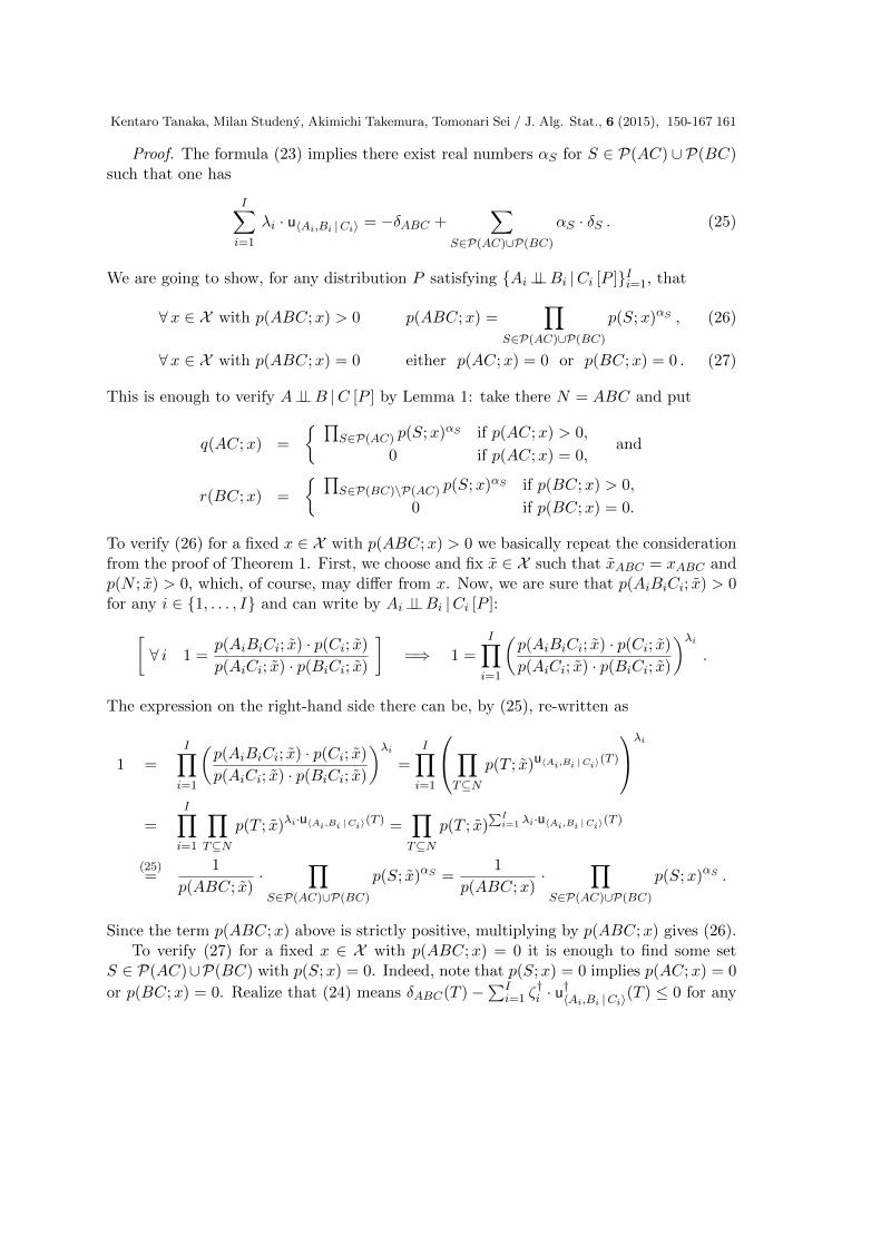
Kentaro Tanaka, Milan Studeny, Akimichi Takemura, Tomonari Sei / J. Alg. Stat., 6 (2015), 150-167 161
Proof. The formula (23) implies there exist real numbers αS for S ∈ P(AC) ∪ P(BC)such that one has
I∑i=1
λi · u〈Ai,Bi |Ci〉 = −δABC +∑
S∈P(AC)∪P(BC)
αS · δS . (25)
We are going to show, for any distribution P satisfying {Ai⊥⊥Bi |Ci [P ]}Ii=1, that
∀x ∈ X with p(ABC;x) > 0 p(ABC;x) =∏
S∈P(AC)∪P(BC)
p(S;x)αS , (26)
∀x ∈ X with p(ABC;x) = 0 either p(AC;x) = 0 or p(BC;x) = 0 . (27)
This is enough to verify A⊥⊥B |C [P ] by Lemma 1: take there N = ABC and put
q(AC;x) =
{ ∏S∈P(AC) p(S;x)αS if p(AC;x) > 0,
0 if p(AC;x) = 0,and
r(BC;x) =
{ ∏S∈P(BC)\P(AC) p(S;x)αS if p(BC;x) > 0,
0 if p(BC;x) = 0.
To verify (26) for a fixed x ∈ X with p(ABC;x) > 0 we basically repeat the considerationfrom the proof of Theorem 1. First, we choose and fix x ∈ X such that xABC = xABC andp(N ; x) > 0, which, of course, may differ from x. Now, we are sure that p(AiBiCi; x) > 0for any i ∈ {1, . . . , I} and can write by Ai⊥⊥Bi |Ci [P ]:[
∀ i 1 =p(AiBiCi; x) · p(Ci; x)
p(AiCi; x) · p(BiCi; x)
]=⇒ 1 =
I∏i=1
(p(AiBiCi; x) · p(Ci; x)
p(AiCi; x) · p(BiCi; x)
)λi.
The expression on the right-hand side there can be, by (25), re-written as
1 =I∏i=1
(p(AiBiCi; x) · p(Ci; x)
p(AiCi; x) · p(BiCi; x)
)λi=
I∏i=1
∏T⊆N
p(T ; x)u〈Ai,Bi |Ci〉(T )
λi
=I∏i=1
∏T⊆N
p(T ; x)λi·u〈Ai,Bi |Ci〉(T ) =∏T⊆N
p(T ; x)∑I
i=1 λi·u〈Ai,Bi |Ci〉(T )
(25)=
1
p(ABC; x)·
∏S∈P(AC)∪P(BC)
p(S; x)αS =1
p(ABC;x)·
∏S∈P(AC)∪P(BC)
p(S;x)αS .
Since the term p(ABC;x) above is strictly positive, multiplying by p(ABC;x) gives (26).To verify (27) for a fixed x ∈ X with p(ABC;x) = 0 it is enough to find some set
S ∈ P(AC)∪P(BC) with p(S;x) = 0. Indeed, note that p(S;x) = 0 implies p(AC;x) = 0
or p(BC;x) = 0. Realize that (24) means δABC(T )−∑I
i=1 ζ†i · u
†〈Ai,Bi |Ci〉(T ) ≤ 0 for any
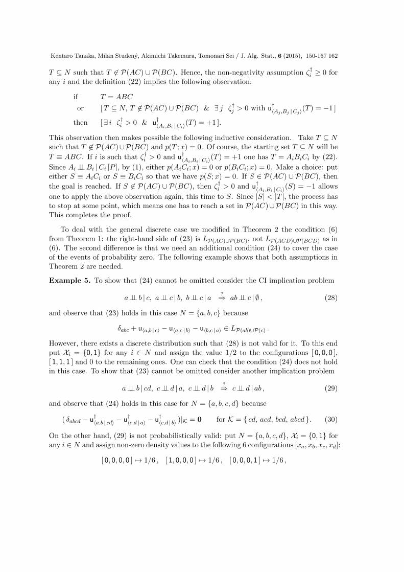
Kentaro Tanaka, Milan Studeny, Akimichi Takemura, Tomonari Sei / J. Alg. Stat., 6 (2015), 150-167 162
T ⊆ N such that T 6∈ P(AC) ∪ P(BC). Hence, the non-negativity assumption ζ†i ≥ 0 forany i and the definition (22) implies the following observation:
if T = ABC
or [T ⊆ N, T 6∈ P(AC) ∪ P(BC) & ∃ j ζ†j > 0 with u†〈Aj ,Bj |Cj〉(T ) = −1 ]
then [ ∃ i ζ†i > 0 & u†〈Ai,Bi |Ci〉(T ) = +1 ].
This observation then makes possible the following inductive consideration. Take T ⊆ Nsuch that T 6∈ P(AC)∪P(BC) and p(T ;x) = 0. Of course, the starting set T ⊆ N will be
T ≡ ABC. If i is such that ζ†i > 0 and u†〈Ai,Bi |Ci〉(T ) = +1 one has T = AiBiCi by (22).
Since Ai⊥⊥Bi |Ci [P ], by (1), either p(AiCi;x) = 0 or p(BiCi;x) = 0. Make a choice: puteither S ≡ AiCi or S ≡ BiCi so that we have p(S;x) = 0. If S ∈ P(AC) ∪ P(BC), then
the goal is reached. If S 6∈ P(AC) ∪ P(BC), then ζ†i > 0 and u†〈Ai,Bi |Ci〉(S) = −1 allows
one to apply the above observation again, this time to S. Since |S| < |T |, the process hasto stop at some point, which means one has to reach a set in P(AC)∪P(BC) in this way.This completes the proof.
To deal with the general discrete case we modified in Theorem 2 the condition (6)from Theorem 1: the right-hand side of (23) is LP(AC)∪P(BC), not LP(ACD)∪P(BCD) as in(6). The second difference is that we need an additional condition (24) to cover the caseof the events of probability zero. The following example shows that both assumptions inTheorem 2 are needed.
Example 5. To show that (24) cannot be omitted consider the CI implication problem
a⊥⊥ b | c, a⊥⊥ c | b, b⊥⊥ c | a ?⇒ ab⊥⊥ c | ∅ , (28)
and observe that (23) holds in this case N = {a, b, c} because
δabc + u〈a,b | c〉 − u〈a,c | b〉 − u〈b,c | a〉 ∈ LP(ab)∪P(c) .
However, there exists a discrete distribution such that (28) is not valid for it. To this endput Xi = {0, 1} for any i ∈ N and assign the value 1/2 to the configurations [ 0, 0, 0 ],[ 1, 1, 1 ] and 0 to the remaining ones. One can check that the condition (24) does not holdin this case. To show that (23) cannot be omitted consider another implication problem
a⊥⊥ b | cd, c⊥⊥ d | a, c⊥⊥ d | b ?⇒ c⊥⊥ d | ab , (29)
and observe that (24) holds in this case for N = {a, b, c, d} because
( δabcd − u†〈a,b | cd〉 − u†〈c,d | a〉 − u†〈c,d | b〉 )|K = 0 for K = { cd, acd, bcd, abcd }. (30)
On the other hand, (29) is not probabilistically valid: put N = {a, b, c, d}, Xi = {0, 1} forany i ∈ N and assign non-zero density values to the following 6 configurations [xa, xb, xc, xd]:
[ 0, 0, 0, 0 ] 7→ 1/6 , [ 1, 0, 0, 0 ] 7→ 1/6 , [ 0, 0, 0, 1 ] 7→ 1/6 ,
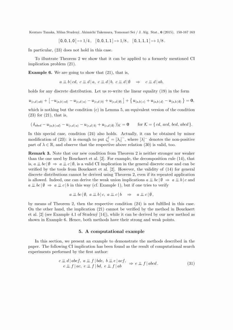
Kentaro Tanaka, Milan Studeny, Akimichi Takemura, Tomonari Sei / J. Alg. Stat., 6 (2015), 150-167 163
[ 0, 0, 1, 0 ] 7→ 1/4 , [ 0, 0, 1, 1 ] 7→ 1/8 , [ 0, 1, 1, 1 ] 7→ 1/8 .
In particular, (23) does not hold in this case.
To illustrate Theorem 2 we show that it can be applied to a formerly mentioned CIimplication problem (21).
Example 6. We are going to show that (21), that is,
a⊥⊥ b | cd, c⊥⊥ d | a, c⊥⊥ d | b, c⊥⊥ d | ∅ ⇒ c⊥⊥ d | ab,
holds for any discrete distribution. Let us re-write the linear equality (19) in the form
u〈c,d | ab〉 +[−u〈a,b | cd〉 − u〈c,d | a〉 − u〈c,d | b〉 + u〈c,d | ∅〉
]+{u〈a,b | c〉 + u〈a,b | d〉 − u〈a,b | ∅〉
}= 0,
which is nothing but the condition (c) in Lemma 5, an equivalent version of the condition(23) for (21), that is,
( δabcd − u〈a,b | cd〉 − u〈c,d | a〉 − u〈c,d | b〉 + u〈c,d | ∅〉 )|K = 0 for K = { cd, acd, bcd, abcd }.
In this special case, condition (24) also holds. Actually, it can be obtained by minor
modification of (23): it is enough to put ζ†i = [λi]−, where [λ]− denotes the non-positive
part of λ ∈ R, and observe that the respective above relation (30) is valid, too.
Remark 3. Note that our new condition from Theorem 2 is neither stronger nor weakerthan the one used by Bouckaert et al. [2]. For example, the decomposition rule (14), thatis, a⊥⊥ bc | ∅ ⇒ a⊥⊥ c | ∅, is a valid CI implication in the general discrete case and can beverified by the tools from Bouckaert et al. [2]. However, the validity of (14) for generaldiscrete distributions cannot be derived using Theorem 2, even if its repeated applicationis allowed. Indeed, one can derive the weak union implications a⊥⊥ bc | ∅ ⇒ a⊥⊥ b | c anda⊥⊥ bc | ∅ ⇒ a⊥⊥ c | b in this way (cf. Example 1), but if one tries to verify
a⊥⊥ bc | ∅, a⊥⊥ b | c, a⊥⊥ c | b ⇒ a⊥⊥ c | ∅ ,
by means of Theorem 2, then the respective condition (24) is not fulfilled in this case.On the other hand, the implication (21) cannot be verified by the method in Bouckaertet al. [2] (see Example 4.1 of Studeny [14]), while it can be derived by our new method asshown in Example 6. Hence, both methods have their strong and weak points.
5. A computational example
In this section, we present an example to demonstrate the methods described in thepaper. The following CI implication has been found as the result of computational searchexperiments performed by the first author:
c⊥⊥ d | abef, a⊥⊥ f | bde, b⊥⊥ e | acf,e⊥⊥ f | ac, e⊥⊥ f | bd, e⊥⊥ f | ab ⇒ e⊥⊥ f | abcd . (31)

Kentaro Tanaka, Milan Studeny, Akimichi Takemura, Tomonari Sei / J. Alg. Stat., 6 (2015), 150-167 164
We found this example by a random search combined with some heuristics. In this search,the set of CI statements in the left-hand side of (31) is given by adding CI statementswhich may factorize a density of a, b, c, d, e, f to functions of a, b, c, d, e and a, b, c, d, f .The above example involves six variables: N = {a, b, c, d, e, f}. While the CI structuresin case |N | ≤ 5 have been studied in detail in Studeny et al. [16] and Hemmecke et al. [6],only a little bit is known about the case |N | ≥ 6.
As we show below, the implication (31) is true. On the other hand, the methodpresented by Bouckaert et al. [2] does not allow one to verify (31). Furthermore, usingthe algorithm by Baioletti et al. [1], one can observe that (31) is not implied by thegraphoid properties, which are well-known valid CI implications in the case of strictlypositive distributions.
We consider the application of the method of Theorem 2. In case of (31), the class Kfrom Lemma 5(b) consists of the supersets of ef and the condition (23) is fulfilled because
( δabcdef − u〈c,d | abef〉 − u〈a,f | bde〉 − u〈b,e | acf〉 − u〈e,f | ac〉 − u〈e,f | bd〉 + u〈e,f | ab〉 )|K = 0. (32)
In particular, the implication (31) holds for any discrete distribution with a strictly positivedensity. Nevertheless, one can also verify the condition (24) in this case, specifically:
( δabcdef − u†〈c,d | abef〉 − u†〈a,f | bde〉 − u†〈b,e | acf〉 − u†〈e,f | ac〉 − u†〈e,f | bd〉 )|K = 0. (33)
Therefore, by Theorem 2, the implication (31) is valid for any discrete distribution.
Remark 4. We can also verify (32) by means of Lemma 5(c). Specifically, one candecompose a multiple by 10 of the respective imset as follows:
10 · u〈e,f | abcd〉+[−10 · u〈c,d | abef〉 − 10 · u〈a,f | bde〉 − 10 · u〈b,e | acf〉− 10 · u〈e,f | ac〉 − 10 · u〈e,f | bd〉 + 10 · u〈e,f | ab〉]
+{
2 · u〈a,b | ∅〉 + 5 · u〈c,d | ∅〉 + u〈c,f | ∅〉 + 3 · u〈c,e | ab〉+ 7 · u〈a,d | c〉 + 9 · u〈b,d | ac〉 + 7 · u〈b,e | ac〉 + u〈d,f | bc〉 + 10 · u〈d,e | abc〉 + 9 · u〈d,f | abc〉+ 6 · u〈a,e | d〉 + 5 · u〈b,e | ad〉 + 10 · u〈a,f | bd〉 + u〈b,f | cd〉 + 5 · u〈b,c | e〉 + 3 · u〈c,d | ae〉+ 2 · u〈c,d | be〉 + u〈a,d | bf〉 + u〈a,c | bdf〉
− 3 · u〈a,e | ∅〉 − 4 · u〈b,c | ∅〉 − u〈b,f | ∅〉 − u〈b,c | a〉 − 3 · u〈c,e | b〉 − u〈c,f | ab〉
− 5 · u〈d,e | ab〉 − 10 · u〈d,f | ab〉 − 5 · u〈d,e | c〉 − u〈a,c | d〉 − 3 · u〈a,e | cd〉− 2 · u〈b,e | cd〉 − 8 · u〈b,d | e〉 − 8 · u〈a,d | be〉 − 2 · u〈a,b | de〉 − u〈b,d | cf〉
}= 0, (34)
where the imsets in the curly brackets in the above equation (34) correspond to additionalconditional independence statements not bridging between e and f . Furthermore, from(34) we have
10 · u〈c,d | abef〉 + 10 · u〈a,f | bde〉 + 10 · u〈b,e | acf〉 + 10 · u〈e,f | ac〉 + 10 · u〈e,f | bd〉+ 3 · u〈a,e | ∅〉 + 4 · u〈b,c | ∅〉 + u〈b,f | ∅〉 + u〈b,c | a〉 + 3 · u〈c,e | b〉 + u〈c,f | ab〉

Kentaro Tanaka, Milan Studeny, Akimichi Takemura, Tomonari Sei / J. Alg. Stat., 6 (2015), 150-167 165
+ 5 · u〈d,e | ab〉 + 10 · u〈d,f | ab〉 + 5 · u〈d,e | c〉 + u〈a,c | d〉 + 3 · u〈a,e | cd〉+ 2 · u〈b,e | cd〉 + 8 · u〈b,d | e〉 + 8 · u〈a,d | be〉 + 2 · u〈a,b | de〉 + u〈b,d | cf〉
= 10 · u〈e,f | abcd〉 + 10 · u〈e,f | ab〉 + 2 · u〈a,b | ∅〉 + 5 · u〈c,d | ∅〉 + u〈c,f | ∅〉 + 3 · u〈c,e | ab〉+ 7 · u〈a,d | c〉 + 9 · u〈b,d | ac〉 + 7 · u〈b,e | ac〉 + u〈d,f | bc〉 + 10 · u〈d,e | abc〉 + 9 · u〈d,f | abc〉+ 6 · u〈a,e | d〉 + 5 · u〈b,e | ad〉 + 10 · u〈a,f | bd〉 + u〈b,f | cd〉 + 5 · u〈b,c | e〉 + 3 · u〈c,d | ae〉+ 2 · u〈c,d | be〉 + u〈a,d | bf〉 + u〈a,c | bdf〉 . (35)
From (35) and the properties of structural imsets (Studeny [15], Hemmecke et al. [6]),we obtain the following implication as a byproduct of the result.
c⊥⊥ d | abef,a⊥⊥ f | bde, b⊥⊥ e | acf, e⊥⊥ f | ac,
e⊥⊥ f | bd, a⊥⊥ e | ∅, b⊥⊥ c | ∅, b⊥⊥ f | ∅,b⊥⊥ c | a, c⊥⊥ e | b,c⊥⊥ f | ab, d⊥⊥ e | ab,
d⊥⊥ f | ab, d⊥⊥ e | c, a⊥⊥ c | d, a⊥⊥ e | cd,b⊥⊥ e | cd, b⊥⊥ d | e, a⊥⊥ d | be, a⊥⊥ b | de,
b⊥⊥ d | cf
⇔
e⊥⊥ f | abcd,e⊥⊥ f | ab, a⊥⊥ b | ∅, c⊥⊥ d | ∅,
c⊥⊥ f | ∅, c⊥⊥ e | ab, a⊥⊥ d | c, b⊥⊥ d | ac,b⊥⊥ e | ac, d⊥⊥ f | bc,d⊥⊥ e | abc, d⊥⊥ f | abc,
a⊥⊥ e | d, b⊥⊥ e | ad, a⊥⊥ f | bd, b⊥⊥ f | cd,b⊥⊥ c | e, c⊥⊥ d | ae, c⊥⊥ d | be, a⊥⊥ d | bf,
a⊥⊥ c | bdf.
Conclusions
Let us summarize the contributions of this note. We have proposed a new linear-algebraic method for derivation of (probabilistic) CI implications. The method mainlyapplies in the case of strictly positive discrete distributions, but it is also extended tothe general case of discrete distributions. The method, which goes beyond the formerlyknown methods, has been illustrated by a few examples. The most complicated one hasbeen obtained as the result of computational experiments.
The reader familiar with algebraic statistics knows that CI implication tasks can oftenbe re-formulated in terms of (ideals of) polynomial rings. For example, the conditionalindependence ideal defined in § 3.1 of Drton et al. [3] consists of polynomials whose indeter-minates correspond to configurations in the (fixed) joint sample space. Another approachis applied in § 5 of Hemmecke et al. [6], where the respective toric ideal consists of poly-nomials whose indeterminates correspond to elementary CI statements i⊥⊥ j |K. Theelements of the Markov basis for that toric ideal seem to correspond to CI implicationsthat can be derived by the method of structural imsets described in Bouckaert et al. [2].Hemmecke et al. [6] obtained 75,889 instances of CI implications (= elements of a minimalMarkov basis) for |N | = 5, which decompose into 1,381 permutation equivalence classes(Kashimura et al. [7]).
The reader may wonder whether the condition (b), respectively (c), of Lemma 3 canalso be modelled/represented in terms of polynomials, that is, by means of binomial re-lations. Perhaps there is a way to do that if one somehow considers Laurent polyno-

REFERENCES 166
mials whose indeterminates correspond to subsets of the set of variables N . To illus-trate this rough idea, consider the CI problem (13) from Example 2 and assume thattabc, tbc, tac, tab, tc, tb, ta, t∅ are the indeterminates. Then the inputs a⊥⊥ b | c, a⊥⊥ c | b andthe output a⊥⊥ c | ∅ are represented as z〈a,b | c〉 ≡ tabctct
−1ac t−1bc , z〈a,c | b〉 ≡ tabctbt
−1ab t−1bc and
z〈a,c | ∅〉 ≡ tact∅t−1a t−1c , respectively. One can model the restriction to K = {ac, abc} in
the condition (b) of Lemma 3 by settings tbc = tab = tc = tb = ta = t∅ = 1. Thus, onehas z〈a,b | c〉|K = tabct
−1ac , z〈a,c | b〉|K = tabc and z〈a,c | ∅〉|K = tac. Then one can introduce a
binomial relation (z〈a,b | c〉|K)−1 · z〈a,c | b〉|K − z〈a,c | ∅〉|K = 0, which can, perhaps, be viewedas a kind of translation/interpretation of the condition (b) from Lemma 3 in the world ofpolynomials.
Acknowledgments
The research of Kentaro Tanaka has been supported by JSPS KAKENHI Grant Num-ber 24700274. The research of Milan Studeny has been supported from the grant projectGACR number 13-20012S. The research of Akimichi Takemura has been supported byJSPS KAKENHI Grant Number 25220001.
References
[1] Marco Baioletti, Giuseppe Busanello, and Barbara Vantaggi. Conditional indepen-dence structure and its closure: Inferential rules and algorithms. International Journalof Approximate Reasoning, 50:1097–1114, 2009.
[2] Remco Bouckaert, Raymond Hemmecke, Silvia Lindner, and Milan Studeny. Efficientalgorithms for conditional independence inference. Journal of Machine Learning Re-search, 11:3453–3479, 2010.
[3] Mathias Drton, Bernd Sturmfels, and Seth Sullivant. Lectures on Algebraic Statistics.Oberwolfach Seminars 39. Birkhauser, Basel, 2009.
[4] Dan Geiger, Azaria Paz, and Judea Pearl. Axioms and algorithms for inferences in-volving probabilistic independence. Information and Computation, 91:128–141, 1991.
[5] Dan Geiger and Judea Pearl. Logical and algorithmic properties of conditional inde-pendence and graphical models. The Annals of Statistics, 21:2001–2021, 1993.
[6] Raymond Hemmecke, Jason Morton, Anne Shiu, Bernd Sturmfels, and Oliver Wien-and. Three counter-examples on semi-graphoids. Combinatorics, Probability andComputing, 17:239–257, 2008.
[7] Takuya Kashimura, Tomonari Sei, Akimichi Takemura, and Kentaro Tanaka. Conesof elementary imsets and supermodular functions: a review and some new results.In Proceedings of the Second CREST-SBM International Conference “Harmony ofGrobner Bases and the Modern Industrial Society”, pages 117–152, 2012.
REFERENCES 167
[8] Francesco M. Malvestuto. A unique formal system for binary decomposition ofdatabase relations, probability distributions and graphs. Information Sciences, 59:21–52, 1992.
[9] Francesco M. Malvestuto and Milan Studeny. Comment on “a unique formal systemfor binary decomposition of database relations, probability distributions and graphs”.Information Sciences, 63:1–2, 1992.
[10] Frantisek Matus. Stochastic independence, algebraic independence and abstract con-nectedness. Theoretical Computer Science, 134:455–471, 1994.
[11] Mathias Niepert, Dirk Van Gucht, and Marc Gyssens. Logical and algorithmic prop-erties of stable conditional independence. International Journal of Approximate Rea-soning, 51:531–543, 2010.
[12] Judea Pearl and Azaria Paz. Graphoids, graph-based logic for reasoning about rele-vance relations. In L. Steels B. Du Boulay, D. Hogg, editor, In Advances in ArtificialIntelligence, Volume II, pages 357–363, North-Holland, 1987.
[13] Wolfgang Spohn. On the properties of conditional independence. In Paul Humphreys,editor, Patrick Suppes, Scientific Philosopher, Volume 1, Probability and ProbabilisticCausality, pages 173–196. Kluwer, 1994.
[14] Milan Studeny. Conditional independence relations have no finite complete charac-terization. In J. A. Vısek S. Kubık, editor, Information Theory, Statistical DecisionFunctions and Random Processes, Transactions of the 11th Prague Conference, Vol-ume B, pages 377–396. Kluwer, 1992.
[15] Milan Studeny. Probabilistic Conditional Independence Structures. Springer-Verlag,London, 2005.
[16] Milan Studeny, Remco R. Bouckaert, and Tomas Kocka. Extreme supermodular setfunctions over five variables. Research report 1977, Institute of Information Theoryand Automation, Prague, 2000.