Model-Powered Conditional Independence Test

Rajat Sen1,*, Ananda Theertha Suresh2,*, Karthikeyan Shanmugam3,*, Alexandros G. Dimakis1, andSanjay Shakkottai1

1The University of Texas at Austin2Google, New York

3IBM Research, Thomas J. Watson Center

Abstract

We consider the problem of non-parametric Conditional Independence testing(CI testing) for continuous random variables. Given i.i.d samples from the jointdistribution f(x, y, z) of continuous random vectors X, Y and Z, we determinewhether X ?? Y |Z. We approach this by converting the conditional independencetest into a classification problem. This allows us to harness very powerful classifierslike gradient-boosted trees and deep neural networks. These models can handlecomplex probability distributions and allow us to perform significantly bettercompared to the prior state of the art, for high-dimensional CI testing. The maintechnical challenge in the classification problem is the need for samples fromthe conditional product distribution fCI

(x, y, z) = f(x|z)f(y|z)f(z) – the jointdistribution if and only if X ?? Y |Z. – when given access only to i.i.d. samplesfrom the true joint distribution f(x, y, z). To tackle this problem we propose a novelnearest neighbor bootstrap procedure and theoretically show that our generatedsamples are indeed close to fCI in terms of total variational distance. We thendevelop theoretical results regarding the generalization bounds for classification forour problem, which translate into error bounds for CI testing. We provide a novelanalysis of Rademacher type classification bounds in the presence of non-i.i.d near-independent samples. We empirically validate the performance of our algorithm onsimulated and real datasets and show performance gains over previous methods.

1 Introduction

Testing datasets for Conditional Independence (CI) have significant applications in several statisti-cal/learning problems; among others, examples include discovering/testing for edges in Bayesiannetworks [15, 27, 7, 9], causal inference [23, 14, 29, 5] and feature selection through Markov Blan-kets [16, 31]. Given a triplet of random variables/vectors (X, Y, Z), we say that X is conditionallyindependent of Y given Z (denoted by X ?? Y |Z), if the joint distribution f

X,Y,Z

(x, y, z) factorizesas f

X,Y,Z

(x, y, z) = fX|Z(x|z)f

Y |Z(y|z)fZ

(z). The problem of Conditional Independence Testing(CI Testing) can be defined as follows: Given n i.i.d samples from f

X,Y,Z

(x, y, z), distinguishbetween the two hypothesis H0 : X ?? Y |Z and H1 : X 6?? Y |Z.

In this paper we propose a data-driven Model-Powered CI test. The central idea in a model-drivenapproach is to convert a statistical testing or estimation problem into a pipeline that utilizes the powerof supervised learning models like classifiers and regressors; such pipelines can then leverage recentadvances in classification/regression in high-dimensional settings. In this paper, we take such amodel-powered approach (illustrated in Fig. 1), which reduces the problem of CI testing to BinaryClassification. Specifically, the key steps of our procedure are as follows:

* Equal Contribution

31st Conference on Neural Information Processing Systems (NIPS 2017), Long Beach, CA, USA.

X Y Zx1 y1 z1

.

.

.

X Y Z.

.

.

Original Samples

X Y Z

.

.

.

X Y Z.

.

.

`1

.

.

.

1

+

`.

.

.

0

0

+

Shu�e

Training

Set

Test

Set

G

g (Trained Classifier)

L(g, De

) (Test Error)

De

Dr

3n Original

Samples

n

2n Original

Samples

Nearest

Neighbor

Bootstrap

U 02

U1

n samples

close to fCI

x3n

y3n

z3n

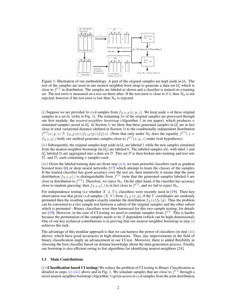
Figure 1: Illustration of our methodology. A part of the original samples are kept aside in U1. Therest of the samples are used in our nearest neighbor boot-strap to generate a data-set U 0

2 which isclose to fCI in distribution. The samples are labeled as shown and a classifier is trained on a trainingset. The test error is measured on a test set there-after. If the test-error is close to 0.5, then H0 is notrejected, however if the test error is low then H0 is rejected.

(i) Suppose we are provided 3n i.i.d samples from fX,Y,Z

(x, y, z). We keep aside n of these originalsamples in a set U1 (refer to Fig. 1). The remaining 2n of the original samples are processed throughour first module, the nearest-neighbor bootstrap (Algorithm 1 in our paper), which produces nsimulated samples stored in U 0

2. In Section 3, we show that these generated samples in U 02 are in fact

close in total variational distance (defined in Section 3) to the conditionally independent distributionfCI

(x, y, z) , fX|Z(x|z)f

Y |Z(y|z)fZ

(z). (Note that only under H0 does the equality fCI

(.) =

fX,Y,Z

(.) hold; our method generates samples close to fCI

(x, y, z) under both hypotheses).

(ii) Subsequently, the original samples kept aside in U1 are labeled 1 while the new samples simulatedfrom the nearest-neighbor bootstrap (in U 0

2) are labeled 0. The labeled samples (U1 with label 1 andU 0

2 labeled 0) are aggregated into a data-set D. This set D is then broken into training and test setsD

r

and De

each containing n samples each.

(iii) Given the labeled training data-set (from step (ii)), we train powerful classifiers such as gradientboosted trees [6] or deep neural networks [17] which attempt to learn the classes of the samples.If the trained classifier has good accuracy over the test set, then intuitively it means that the jointdistribution f

X,Y,Z

(.) is distinguishable from fCI (note that the generated samples labeled 0 areclose in distribution to fCI ). Therefore, we reject H0. On the other hand, if the classifier has accuracyclose to random guessing, then f

X,Y,Z

(.) is in fact close to fCI , and we fail to reject H0.

For independence testing (i.e whether X ?? Y ), classifiers were recently used in [19]. Their keyobservation was that given i.i.d samples (X, Y ) from f

X,Y

(x, y), if the Y coordinates are randomlypermuted then the resulting samples exactly emulate the distribution f

X

(x)fY

(y). Thus the problemcan be converted to a two sample test between a subset of the original samples and the other subsetwhich is permuted - Binary classifiers were then harnessed for this two-sample testing; for detailssee [19]. However, in the case of CI testing we need to emulate samples from fCI . This is harderbecause the permutation of the samples needs to be Z dependent (which can be high-dimensional).One of our key technical contributions is in proving that our nearest-neighbor bootstrap in step (i)achieves this task.

The advantage of this modular approach is that we can harness the power of classifiers (in step (iii)above), which have good accuracies in high-dimensions. Thus, any improvements in the field ofbinary classification imply an advancement in our CI test. Moreover, there is added flexibility inchoosing the best classifier based on domain knowledge about the data-generation process. Finally,our bootstrap is also efficient owing to fast algorithms for identifying nearest-neighbors [24].

1.1 Main Contributions

(i) (Classification based CI testing) We reduce the problem of CI testing to Binary Classification asdetailed in steps (i)-(iii) above and in Fig. 1. We simulate samples that are close to fCI through anovel nearest-neighbor bootstrap (Algorithm 1) given access to i.i.d samples from the joint distribution.

2

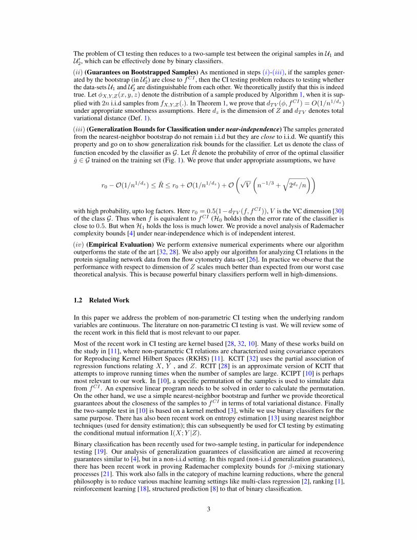
The problem of CI testing then reduces to a two-sample test between the original samples in U1 andU 0

2, which can be effectively done by binary classifiers.

(ii) (Guarantees on Bootstrapped Samples) As mentioned in steps (i)-(iii), if the samples gener-ated by the bootstrap (in U 0

2) are close to fCI , then the CI testing problem reduces to testing whetherthe data-sets U1 and U 0

2 are distinguishable from each other. We theoretically justify that this is indeedtrue. Let �

X,Y,Z

(x, y, z) denote the distribution of a sample produced by Algorithm 1, when it is sup-plied with 2n i.i.d samples from f

X,Y,Z

(.). In Theorem 1, we prove that dTV

(�, fCI

) = O(1/n1/d

z

)

under appropriate smoothness assumptions. Here dz

is the dimension of Z and dTV

denotes totalvariational distance (Def. 1).

(iii) (Generalization Bounds for Classification under near-independence) The samples generatedfrom the nearest-neighbor bootstrap do not remain i.i.d but they are close to i.i.d. We quantify thisproperty and go on to show generalization risk bounds for the classifier. Let us denote the class offunction encoded by the classifier as G. Let ˆR denote the probability of error of the optimal classifierg 2 G trained on the training set (Fig. 1). We prove that under appropriate assumptions, we have

r0 � O(1/n1/d

z

) ˆR r0 + O(1/n1/d

z

) + O✓p

V

✓n�1/3

+

q2

d

z/n

◆◆

with high probability, upto log factors. Here r0 = 0.5(1�dTV

(f, fCI

)), V is the VC dimension [30]of the class G. Thus when f is equivalent to fCI (H0 holds) then the error rate of the classifier isclose to 0.5. But when H1 holds the loss is much lower. We provide a novel analysis of Rademachercomplexity bounds [4] under near-independence which is of independent interest.

(iv) (Empirical Evaluation) We perform extensive numerical experiments where our algorithmoutperforms the state of the art [32, 28]. We also apply our algorithm for analyzing CI relations in theprotein signaling network data from the flow cytometry data-set [26]. In practice we observe that theperformance with respect to dimension of Z scales much better than expected from our worst casetheoretical analysis. This is because powerful binary classifiers perform well in high-dimensions.

1.2 Related Work

In this paper we address the problem of non-parametric CI testing when the underlying randomvariables are continuous. The literature on non-parametric CI testing is vast. We will review some ofthe recent work in this field that is most relevant to our paper.

Most of the recent work in CI testing are kernel based [28, 32, 10]. Many of these works build onthe study in [11], where non-parametric CI relations are characterized using covariance operatorsfor Reproducing Kernel Hilbert Spaces (RKHS) [11]. KCIT [32] uses the partial association ofregression functions relating X , Y , and Z. RCIT [28] is an approximate version of KCIT thatattempts to improve running times when the number of samples are large. KCIPT [10] is perhapsmost relevant to our work. In [10], a specific permutation of the samples is used to simulate datafrom fCI . An expensive linear program needs to be solved in order to calculate the permutation.On the other hand, we use a simple nearest-neighbor bootstrap and further we provide theoreticalguarantees about the closeness of the samples to fCI in terms of total variational distance. Finallythe two-sample test in [10] is based on a kernel method [3], while we use binary classifiers for thesame purpose. There has also been recent work on entropy estimation [13] using nearest neighbortechniques (used for density estimation); this can subsequently be used for CI testing by estimatingthe conditional mutual information I(X; Y |Z).

Binary classification has been recently used for two-sample testing, in particular for independencetesting [19]. Our analysis of generalization guarantees of classification are aimed at recoveringguarantees similar to [4], but in a non-i.i.d setting. In this regard (non-i.i.d generalization guarantees),there has been recent work in proving Rademacher complexity bounds for �-mixing stationaryprocesses [21]. This work also falls in the category of machine learning reductions, where the generalphilosophy is to reduce various machine learning settings like multi-class regression [2], ranking [1],reinforcement learning [18], structured prediction [8] to that of binary classification.

3

2 Problem Setting and Algorithms

In this section we describe the algorithmic details of our CI testing procedure. We first formallydefine our problem. Then we describe our bootstrap algorithm for generating the data-set that mimicssamples from fCI . We give a detailed pseudo-code for our CI testing process which reduces theproblem to that of binary classification. Finally, we suggest further improvements to our algorithm.

Problem Setting: The problem setting is that of non-parametric Conditional Independence (CI)testing given i.i.d samples from the joint distributions of random variables/vectors [32, 10, 28]. We aregiven 3n i.i.d samples from a continuous joint distribution f

X,Y,Z

(x, y, z) where x 2 Rd

x , y 2 Rd

y

and z 2 Rd

z . The goal is to test whether X ?? Y |Z i.e whether fX,Y,Z

(x, y, z) factorizes as,f

X,Y,Z

(x, y, z) = fX|Z(x|z)f

Y |Z(y|z)fZ

(z) , fCI

(x, y, z)

This is essentially a hypothesis testing problem where: H0 : X ?? Y |Z and H1 : X 6?? Y |Z.

Note: For notational convenience, we will drop the subscripts when the context is evident. Forinstance we may use f(x|z) in place of f

X|Z(x|z).

Nearest-Neighbor Bootstrap: Algorithm 1 is a procedure to generate a data-set U 0 consisting ofn samples given a data-set U of 2n i.i.d samples from the distribution f

X,Y,Z

(x, y, z). The data-setU is broken into two equally sized partitions U1 and U2. Then for each sample in U1, we find thenearest neighbor in U2 in terms of the Z coordinates. The Y -coordinates of the sample from U1 areexchanged with the Y -coordinates of its nearest neighbor (in U2); the modified sample is added to U 0.

Algorithm 1 DataGen - Given data-set U = U1 [ U2 of 2n i.i.d samples from f(x, y, z) (|U1| =

|U2| = n ), returns a new data-set U 0 having n samples.1: function DATAGEN(U1, U2, 2n)2: U 0

= ;3: for u in U1 do4: Let v = (x0, y0, z0

) 2 U2 be the sample such that z0 is the 1-Nearest Neighbor (1-NN)of z (in `2 norm) in the whole data-set U2, where u = (x, y, z)

5: Let u0= (x, y0, z) and U 0

= U 0 [ {u0}.6: end for7: end function

One of our main results is that the samples in U 0, generated in Algorithm 1 mimic samples comingfrom the distribution fCI . Suppose u = (x, y, z) 2 U1 be a sample such that f

Z

(z) is not toosmall. In this case z0 (the 1-NN sample from U2) will not be far from z. Therefore given a fixed z,under appropriate smoothness assumptions, y0 will be close to an independent sample coming fromf

Y |Z(y|z0) ⇠ f

Y |Z(y|z). On the other hand if fZ

(z) is small, then z is a rare occurrence and willnot contribute adversely.

CI Testing Algorithm: Now we introduce our CI testing algorithm, which uses Algorithm 1 alongwith binary classifiers. The psuedo-code is in Algorithm 2 (Classifier CI Test -CCIT).

Algorithm 2 CCITv1 - Given data-set U of 3n i.i.d samples from f(x, y, z), returns if X ?? Y |Z.1: function CCIT(U , 3n, ⌧, G)2: Partition U into three disjoint partitions U1, U2 and U3 of size n each, randomly.3: Let U 0

2 = DataGen(U2, U3, 2n) (Algorithm 1). Note that |U 02| = n.

4: Create Labeled data-set D := {(u, ` = 1)}u2U1 [ {(u0, `0

= 0)}u

02U 02

5: Divide data-set D into train and test set Dr

and De

respectively. Note that |Dr

| = |De

| = n.6: Let g = argmin

g2GˆL(g, D

r

) :=

1|D

r

|P

(u,`)2Dr

1{g(u) 6= l}. This is Empirical RiskMinimization for training the classifier (finding the best function in the class G).

7: If ˆL(g, De

) > 0.5 � ⌧ , then conclude X ?? Y |Z, otherwise, conclude X 6?? Y |Z.8: end function

4

In Algorithm 2, the original samples in U1 and the nearest-neighbor bootstrapped samples in U 02

should be almost indistinguishable if H0 holds. However, if H1 holds, then the classifier trained inLine 6 should be able to easily distinguish between the samples corresponding to different labels. InLine 6, G denotes the space of functions over which risk minimization is performed in the classifier.

We will show (in Theorem 1) that the variational distance between the distribution of one of thesamples in U 0

2 and fCI

(x, y, z) is very small for large n. However, the samples in U 02 are not

exactly i.i.d but close to i.i.d. Therefore, in practice for finite n, there is a small bias b > 0 i.e.ˆL(g, D

e

) ⇠ 0.5 � b, even when H0 holds. The threshold ⌧ needs to be greater than b in order forAlgorithm 2 to function. In the next section, we present an algorithm where this bias is corrected.

Algorithm with Bias Correction: We present an improved bias-corrected version of our algorithmas Algorithm 3. As mentioned in the previous section, in Algorithm 2, the optimal classifier may beable to achieve a loss slightly less that 0.5 in the case of finite n, even when H0 is true. However, theclassifier is expected to distinguish between the two data-sets only based on the Y, Z coordinates, asthe joint distribution of X and Z remains the same in the nearest-neighbor bootstrap. The key ideain Algorithm 3 is to train a classifier only using the Y and Z coordinates, denoted by g0. As beforewe also train another classier using all the coordinates, which is denoted by g. The test loss of g0 isexpected to be roughly 0.5 � b, where b is the bias mentioned in the previous section. Therefore, wecan just subtract this bias. Thus, when H0 is true ˆL(g0, D0

e

) � ˆL(g, De

) will be close to 0. However,when H1 holds, then ˆL(g, D

e

) will be much lower, as the classifier g has been trained leveraging theinformation encoded in all the coordinates.

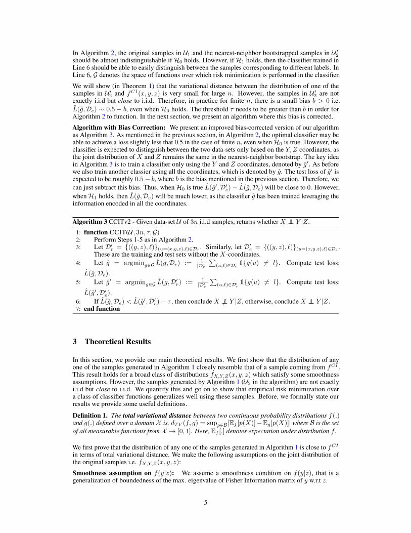
Algorithm 3 CCITv2 - Given data-set U of 3n i.i.d samples, returns whether X ?? Y |Z.1: function CCIT(U , 3n, ⌧, G)2: Perform Steps 1-5 as in Algorithm 2.3: Let D0

r

= {((y, z), `)}(u=(x,y,z),`)2Dr

. Similarly, let D0e

= {((y, z), `)}(u=(x,y,z),`)2De

.These are the training and test sets without the X-coordinates.

4: Let g = argmin

g2GˆL(g, D

r

) :=

1|D

r

|P

(u,`)2Dr

1{g(u) 6= l}. Compute test loss:ˆL(g, D

e

).5: Let g0

= argmin

g2GˆL(g, D0

r

) :=

1|D0

r

|P

(u,`)2D0r

1{g(u) 6= l}. Compute test loss:ˆL(g0, D0

e

).6: If ˆL(g, D

e

) < ˆL(g0, D0e

) � ⌧ , then conclude X 6?? Y |Z, otherwise, conclude X ?? Y |Z.7: end function

3 Theoretical Results

In this section, we provide our main theoretical results. We first show that the distribution of anyone of the samples generated in Algorithm 1 closely resemble that of a sample coming from fCI .This result holds for a broad class of distributions f

X,Y,Z

(x, y, z) which satisfy some smoothnessassumptions. However, the samples generated by Algorithm 1 (U2 in the algorithm) are not exactlyi.i.d but close to i.i.d. We quantify this and go on to show that empirical risk minimization overa class of classifier functions generalizes well using these samples. Before, we formally state ourresults we provide some useful definitions.

Definition 1. The total variational distance between two continuous probability distributions f(.)and g(.) defined over a domain X is, d

TV

(f, g) = sup

p2B|Ef

[p(X)]�Eg

[p(X)]| where B is the setof all measurable functions from X ! [0, 1]. Here, E

f

[.] denotes expectation under distribution f .

We first prove that the distribution of any one of the samples generated in Algorithm 1 is close to fCI

in terms of total variational distance. We make the following assumptions on the joint distribution ofthe original samples i.e. f

X,Y,Z

(x, y, z):

Smoothness assumption on f(y|z): We assume a smoothness condition on f(y|z), that is ageneralization of boundedness of the max. eigenvalue of Fisher Information matrix of y w.r.t z.

5

Assumption 1. For z 2 Rd

z , a such that ka � zk2 ✏1, the generalized curvature matrix Ia

(z) is,

Ia

(z)

ij

=

@2

@z0i

@z0j

Zlog

f(y|z)

f(y|z0)

f(y|z)dy

!�����z

0=a

= E"��2

log f(y|z0)

�z0i

�z0j

���z

0=a

�����Z = z

#(1)

We require that for all z 2 Rd

z and all a such that ka � zk2 ✏1, �max

(Ia

(z)) �. Analogousassumptions have been made on the Hessian of the density in the context of entropy estimation [12].

Smoothness assumptions on f(z): We assume some smoothness properties of the probabilitydensity function f(z). The smoothness assumptions (in Assumption 2) is a subset of the assumptionsmade in [13] (Assumption 1, Page 5) for entropy estimation.Definition 2. For any � > 0, we define G(�) = P (f(Z) �). This is the probability mass of thedistribution of Z in the areas where the p.d.f is less than �.Definition 3. (Hessian Matrix) Let H

f

(z) denote the Hessian Matrix of the p.d.f f(z) with respectto z i.e H

f

(z)

ij

= @2f(z)/@zi

@zj

, provided it is twice continuously differentiable at z.Assumption 2. The probability density function f(z) satisfies the following:

(1) f(z) is twice continuously differentiable and the Hessian matrix Hf

satisfies kHf

(z)k2 cd

z

almost everywhere, where cd

z

is only dependent on the dimension.

(2)R

f(z)

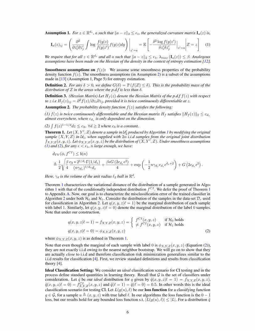
1�1/ddz c3, 8d � 2 where c3 is a constant.Theorem 1. Let (X,Y 0, Z) denote a sample in U 0

2 produced by Algorithm 1 by modifying the originalsample (X, Y, Z) in U1, when supplied with 2n i.i.d samples from the original joint distributionf

X,Y,Z

(x, y, z). Let �X,Y,Z

(x, y, z) be the distribution of (X, Y 0, Z). Under smoothness assumptions(1) and (2), for any ✏ < ✏1, n large enough, we have:

dTV

(�, fCI

) b(n)

, 1

2

s�

4

c3 ⇤ 2

1/d

z

�(1/dz

)

(n�d

z

)

1/d

zdz

+

�✏G (2cd

z

✏2)

4

+ exp

✓�1

2

n�d

z

cd

z

✏d

z

+2

◆+ G

�2c

d

z

✏2�.

Here, �d

is the volume of the unit radius `2 ball in Rd.

Theorem 1 characterizes the variational distance of the distribution of a sample generated in Algo-rithm 1 with that of the conditionally independent distribution fCI . We defer the proof of Theorem 1to Appendix A. Now, our goal is to characterize the misclassification error of the trained classifier inAlgorithm 2 under both H0 and H1. Consider the distribution of the samples in the data-set D

r

usedfor classification in Algorithm 2. Let q(x, y, z|` = 1) be the marginal distribution of each samplewith label 1. Similarly, let q(x, y, z|` = 0) denote the marginal distribution of the label 0 samples.Note that under our construction,

q(x, y, z|` = 1) = fX,Y,Z

(x, y, z) =

⇢fCI

(x, y, z) if H0 holds6= fCI

(x, y, z) if H1 holdsq(x, y, z|` = 0) = �

X,Y,Z

(x, y, z) (2)

where �X,Y,Z

(x, y, z) is as defined in Theorem 1.

Note that even though the marginal of each sample with label 0 is �X,Y,Z

(x, y, z) (Equation (2)),they are not exactly i.i.d owing to the nearest neighbor bootstrap. We will go on to show that theyare actually close to i.i.d and therefore classification risk minimization generalizes similar to thei.i.d results for classification [4]. First, we review standard definitions and results from classificationtheory [4].

Ideal Classification Setting: We consider an ideal classification scenario for CI testing and in theprocess define standard quantities in learning theory. Recall that G is the set of classifiers underconsideration. Let q be our ideal distribution for q given by q(x, y, z|` = 1) = f

X,Y,Z

(x, y, z),q(x, y, z|` = 0) = fCI

X,Y,Z

(x, y, z) and q(` = 1) = q(` = 0) = 0.5. In other words this is the idealclassification scenario for testing CI. Let L(g(u), `) be our loss function for a classifying functiong 2 G, for a sample u , (x, y, z) with true label `. In our algorithms the loss function is the 0 � 1

loss, but our results hold for any bounded loss function s.t. |L(g(u), `)| |L|. For a distribution q

6

and a classifier g let Rq

(g) , Eu,`⇠q

[L(g(u), `)] be the expected risk of the function g. The riskoptimal classifier g⇤

q

under q is given by g⇤q

, arg min

g2G Rq

(g). Similarly for a set of samples S

and a classifier g, let RS

(g) , 1|S|P

u,`2S

L(g(u), `) be the empirical risk on the set of samples.We define g

S

as the classifier that minimizes the empirical loss on the observed set of samples Sthat is, g

S

, arg min

g2G RS

(g).

If the samples in S are generated independently from q, then standard results from the learning theorystates that with probability � 1 � �,

Rq

(gS

) Rq

(g⇤q

) + C

rV

n+

r2 log(1/�)

n, (3)

where V is the VC dimension [30] of the classification model, C is an universal constant and n = |S|.Guarantees under near-independent samples: Our goal is to prove a result like (3), for theclassification problem in Algorithm 2. However, in this case we do not have access to i.i.d samplesbecause the samples in U 0

2 do not remain independent. We will see that they are close to independentin some sense. This brings us to one of our main results in Theorem 2.

Theorem 2. Assume that the joint distribution f(x, y, z) satisfies the conditions in Theorem 1.Further assume that f(z) has a bounded Lipschitz constant. Consider the classifier g in Algorithm 2trained on the set D

r

. Let S = Dr

. Then according to our definition gS

= g. For ✏ > 0 we have:

(i) Rq

(gS

) � Rq

(g⇤q

) �n

, C|L|

pV +

rlog

1

�

! ✓log(n/�)

n

◆1/3

+

r4

d

z

log(n/�) + on

(1/✏)

n

!+ G(✏)

!,

with probability at least 1 � 8�. Here V is the V.C. dimension of the classification function class, G isas defined in Def. 2, C is an universal constant and |L| is the bound on the absolute value of the loss.

(ii) Suppose the loss is L(g(u), `) = 1g(u) 6=`

(s.t |L| 1). Further suppose the class of classifyingfunctions is such that R

q

(g⇤q

) r0 + ⌘. Here, r0 , 0.5(1 � dTV

(q(x, y, z|1), q(x, y, z|0))) is therisk of the Bayes optimal classifier when q(` = 1) = q(` = 0). This is the best loss that any classifiercan achieve for this classification problem [4]. Under this setting, w.p at least 1 � 8� we have:

1

2

�1 � d

TV

(f, fCI

)

�� b(n)

2

Rq

(gS

) 1

2

�1 � d

TV

(f, fCI

)

�+

b(n)

2

+ ⌘ + �n

where b(n) is as defined in Theorem 1.

We prove Theorem 2 as Theorem 3 and Theorem 4 in the appendix. In part (i) of the theoremwe prove that generalization bounds hold even when the samples are not exactly i.i.d. Intuitively,consider two sample inputs u

i

, uj

2 U1, such that corresponding Z coordinates zi

and zj

are faraway. Then we expect the resulting samples u0

i

and u0j

(in U 02) to be nearly-independent. By carefully

capturing this notion of spatial near-independence, we prove generalization errors in Theorem 3. Part(ii) of the theorem essentially implies that the error of the trained classifier will be close to 0.5 (l.h.s)when f ⇠ fCI (under H0). On the other hand under H1 if d

TV

(f, fCI

) > 1 � �, the error will beless than 0.5(� + b(n)) + �

n

which is small.

4 Empirical Results

In this section we provide empirical results comparing our proposed algorithm and other state of theart algorithms. The algorithms under comparison are: (i) CCIT - Algorithm 3 in our paper where weuse XGBoost [6] as the classifier. In our experiments, for each data-set we boot-strap the samples andrun our algorithm B times. The results are averaged over B bootstrap runs1. (ii) KCIT - Kernel CItest from [32]. We use the Matlab code available online. (iii) RCIT - Randomized CI Test from [28].We use the R package that is publicly available.

1The python package for our implementation can be found here (https://github.com/rajatsen91/CCIT).

7

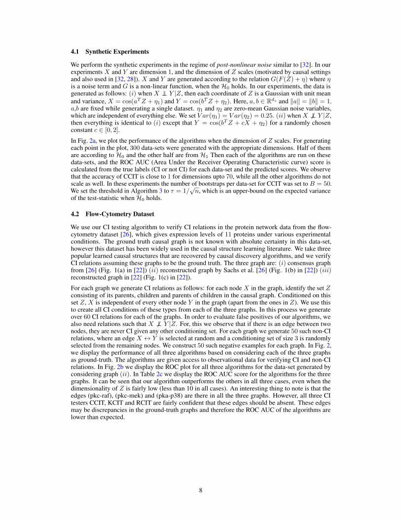
4.1 Synthetic Experiments

We perform the synthetic experiments in the regime of post-nonlinear noise similar to [32]. In ourexperiments X and Y are dimension 1, and the dimension of Z scales (motivated by causal settingsand also used in [32, 28]). X and Y are generated according to the relation G(F (Z) + ⌘) where ⌘is a noise term and G is a non-linear function, when the H0 holds. In our experiments, the data isgenerated as follows: (i) when X ?? Y |Z, then each coordinate of Z is a Gaussian with unit meanand variance, X = cos(aT Z + ⌘1) and Y = cos(bT Z + ⌘2). Here, a, b 2 Rd

z and kak = kbk = 1.a,b are fixed while generating a single dataset. ⌘1 and ⌘2 are zero-mean Gaussian noise variables,which are independent of everything else. We set V ar(⌘1) = V ar(⌘2) = 0.25. (ii) when X 6?? Y |Z,then everything is identical to (i) except that Y = cos(bT Z + cX + ⌘2) for a randomly chosenconstant c 2 [0, 2].

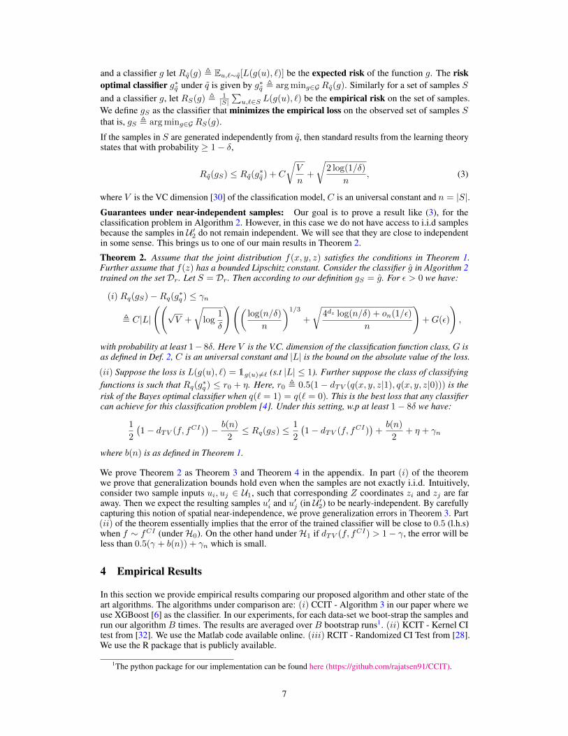
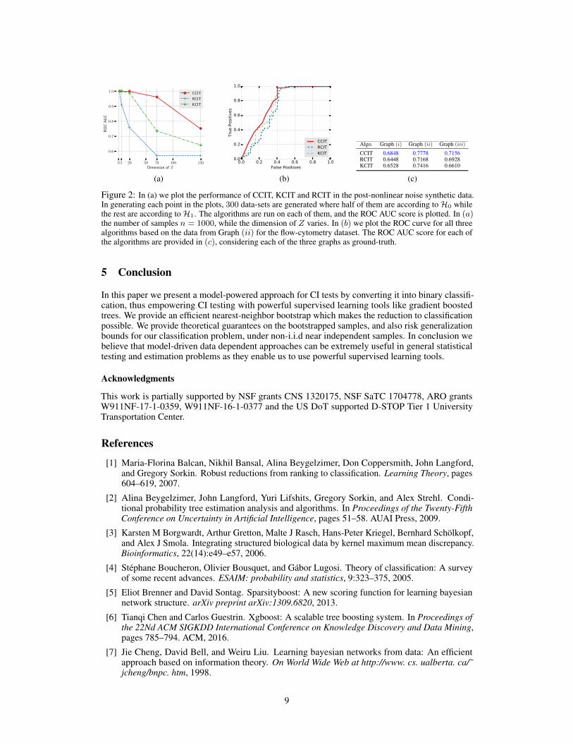
In Fig. 2a, we plot the performance of the algorithms when the dimension of Z scales. For generatingeach point in the plot, 300 data-sets were generated with the appropriate dimensions. Half of themare according to H0 and the other half are from H1 Then each of the algorithms are run on thesedata-sets, and the ROC AUC (Area Under the Receiver Operating Characteristic curve) score iscalculated from the true labels (CI or not CI) for each data-set and the predicted scores. We observethat the accuracy of CCIT is close to 1 for dimensions upto 70, while all the other algorithms do notscale as well. In these experiments the number of bootstraps per data-set for CCIT was set to B = 50.We set the threshold in Algorithm 3 to ⌧ = 1/

pn, which is an upper-bound on the expected variance

of the test-statistic when H0 holds.

4.2 Flow-Cytometry Dataset

We use our CI testing algorithm to verify CI relations in the protein network data from the flow-cytometry dataset [26], which gives expression levels of 11 proteins under various experimentalconditions. The ground truth causal graph is not known with absolute certainty in this data-set,however this dataset has been widely used in the causal structure learning literature. We take threepopular learned causal structures that are recovered by causal discovery algorithms, and we verifyCI relations assuming these graphs to be the ground truth. The three graph are: (i) consensus graphfrom [26] (Fig. 1(a) in [22]) (ii) reconstructed graph by Sachs et al. [26] (Fig. 1(b) in [22]) (iii)reconstructed graph in [22] (Fig. 1(c) in [22]).

For each graph we generate CI relations as follows: for each node X in the graph, identify the set Zconsisting of its parents, children and parents of children in the causal graph. Conditioned on thisset Z, X is independent of every other node Y in the graph (apart from the ones in Z). We use thisto create all CI conditions of these types from each of the three graphs. In this process we generateover 60 CI relations for each of the graphs. In order to evaluate false positives of our algorithms, wealso need relations such that X 6?? Y |Z. For, this we observe that if there is an edge between twonodes, they are never CI given any other conditioning set. For each graph we generate 50 such non-CIrelations, where an edge X $ Y is selected at random and a conditioning set of size 3 is randomlyselected from the remaining nodes. We construct 50 such negative examples for each graph. In Fig. 2,we display the performance of all three algorithms based on considering each of the three graphsas ground-truth. The algorithms are given access to observational data for verifying CI and non-CIrelations. In Fig. 2b we display the ROC plot for all three algorithms for the data-set generated byconsidering graph (ii). In Table 2c we display the ROC AUC score for the algorithms for the threegraphs. It can be seen that our algorithm outperforms the others in all three cases, even when thedimensionality of Z is fairly low (less than 10 in all cases). An interesting thing to note is that theedges (pkc-raf), (pkc-mek) and (pka-p38) are there in all the three graphs. However, all three CItesters CCIT, KCIT and RCIT are fairly confident that these edges should be absent. These edgesmay be discrepancies in the ground-truth graphs and therefore the ROC AUC of the algorithms arelower than expected.

8

0 5 20 50 70 100 150Dimension of Z

0.6

0.7

0.8

0.9

1.0

RO

CAU

C

CCIT

RCIT

KCIT

(a) (b)

Algo. Graph (i) Graph (ii) Graph (iii)

CCIT 0.6848 0.7778 0.7156RCIT 0.6448 0.7168 0.6928KCIT 0.6528 0.7416 0.6610

(c)

Figure 2: In (a) we plot the performance of CCIT, KCIT and RCIT in the post-nonlinear noise synthetic data.In generating each point in the plots, 300 data-sets are generated where half of them are according to H0 whilethe rest are according to H1. The algorithms are run on each of them, and the ROC AUC score is plotted. In (a)the number of samples n = 1000, while the dimension of Z varies. In (b) we plot the ROC curve for all threealgorithms based on the data from Graph (ii) for the flow-cytometry dataset. The ROC AUC score for each ofthe algorithms are provided in (c), considering each of the three graphs as ground-truth.

5 Conclusion

In this paper we present a model-powered approach for CI tests by converting it into binary classifi-cation, thus empowering CI testing with powerful supervised learning tools like gradient boostedtrees. We provide an efficient nearest-neighbor bootstrap which makes the reduction to classificationpossible. We provide theoretical guarantees on the bootstrapped samples, and also risk generalizationbounds for our classification problem, under non-i.i.d near independent samples. In conclusion webelieve that model-driven data dependent approaches can be extremely useful in general statisticaltesting and estimation problems as they enable us to use powerful supervised learning tools.

Acknowledgments

This work is partially supported by NSF grants CNS 1320175, NSF SaTC 1704778, ARO grantsW911NF-17-1-0359, W911NF-16-1-0377 and the US DoT supported D-STOP Tier 1 UniversityTransportation Center.

References[1] Maria-Florina Balcan, Nikhil Bansal, Alina Beygelzimer, Don Coppersmith, John Langford,

and Gregory Sorkin. Robust reductions from ranking to classification. Learning Theory, pages604–619, 2007.

[2] Alina Beygelzimer, John Langford, Yuri Lifshits, Gregory Sorkin, and Alex Strehl. Condi-tional probability tree estimation analysis and algorithms. In Proceedings of the Twenty-FifthConference on Uncertainty in Artificial Intelligence, pages 51–58. AUAI Press, 2009.

[3] Karsten M Borgwardt, Arthur Gretton, Malte J Rasch, Hans-Peter Kriegel, Bernhard Schölkopf,and Alex J Smola. Integrating structured biological data by kernel maximum mean discrepancy.Bioinformatics, 22(14):e49–e57, 2006.

[4] Stéphane Boucheron, Olivier Bousquet, and Gábor Lugosi. Theory of classification: A surveyof some recent advances. ESAIM: probability and statistics, 9:323–375, 2005.

[5] Eliot Brenner and David Sontag. Sparsityboost: A new scoring function for learning bayesiannetwork structure. arXiv preprint arXiv:1309.6820, 2013.

[6] Tianqi Chen and Carlos Guestrin. Xgboost: A scalable tree boosting system. In Proceedings ofthe 22Nd ACM SIGKDD International Conference on Knowledge Discovery and Data Mining,pages 785–794. ACM, 2016.

[7] Jie Cheng, David Bell, and Weiru Liu. Learning bayesian networks from data: An efficientapproach based on information theory. On World Wide Web at http://www. cs. ualberta. ca/˜jcheng/bnpc. htm, 1998.

9

[8] Hal Daumé, John Langford, and Daniel Marcu. Search-based structured prediction. Machinelearning, 75(3):297–325, 2009.

[9] Luis M De Campos and Juan F Huete. A new approach for learning belief networks usingindependence criteria. International Journal of Approximate Reasoning, 24(1):11–37, 2000.

[10] Gary Doran, Krikamol Muandet, Kun Zhang, and Bernhard Schölkopf. A permutation-basedkernel conditional independence test. In UAI, pages 132–141, 2014.

[11] Kenji Fukumizu, Francis R Bach, and Michael I Jordan. Dimensionality reduction for supervisedlearning with reproducing kernel hilbert spaces. Journal of Machine Learning Research,5(Jan):73–99, 2004.

[12] Weihao Gao, Sewoong Oh, and Pramod Viswanath. Breaking the bandwidth barrier: Geometri-cal adaptive entropy estimation. In Advances in Neural Information Processing Systems, pages2460–2468, 2016.

[13] Weihao Gao, Sewoong Oh, and Pramod Viswanath. Demystifying fixed k-nearest neighborinformation estimators. arXiv preprint arXiv:1604.03006, 2016.

[14] Markus Kalisch and Peter Bühlmann. Estimating high-dimensional directed acyclic graphs withthe pc-algorithm. Journal of Machine Learning Research, 8(Mar):613–636, 2007.

[15] Daphne Koller and Nir Friedman. Probabilistic graphical models: principles and techniques.MIT press, 2009.

[16] Daphne Koller and Mehran Sahami. Toward optimal feature selection. Technical report,Stanford InfoLab, 1996.

[17] Alex Krizhevsky, Ilya Sutskever, and Geoffrey E Hinton. Imagenet classification with deepconvolutional neural networks. In Advances in neural information processing systems, pages1097–1105, 2012.

[18] John Langford and Bianca Zadrozny. Reducing t-step reinforcement learning to classification.In Proc. of the Machine Learning Reductions Workshop, 2003.

[19] David Lopez-Paz and Maxime Oquab. Revisiting classifier two-sample tests. arXiv preprintarXiv:1610.06545, 2016.

[20] Colin McDiarmid. On the method of bounded differences. Surveys in combinatorics, 141(1):148–188, 1989.

[21] Mehryar Mohri and Afshin Rostamizadeh. Rademacher complexity bounds for non-iid processes.In Advances in Neural Information Processing Systems, pages 1097–1104, 2009.

[22] Joris Mooij and Tom Heskes. Cyclic causal discovery from continuous equilibrium data. arXivpreprint arXiv:1309.6849, 2013.

[23] Judea Pearl. Causality. Cambridge university press, 2009.[24] V Ramasubramanian and Kuldip K Paliwal. Fast k-dimensional tree algorithms for nearest

neighbor search with application to vector quantization encoding. IEEE Transactions on SignalProcessing, 40(3):518–531, 1992.

[25] Bero Roos. On the rate of multivariate poisson convergence. Journal of Multivariate Analysis,69(1):120–134, 1999.

[26] Karen Sachs, Omar Perez, Dana Pe’er, Douglas A Lauffenburger, and Garry P Nolan.Causal protein-signaling networks derived from multiparameter single-cell data. Science,308(5721):523–529, 2005.

[27] Peter Spirtes, Clark N Glymour, and Richard Scheines. Causation, prediction, and search. MITpress, 2000.

[28] Eric V Strobl, Kun Zhang, and Shyam Visweswaran. Approximate kernel-based conditionalindependence tests for fast non-parametric causal discovery. arXiv preprint arXiv:1702.03877,2017.

[29] Ioannis Tsamardinos, Laura E Brown, and Constantin F Aliferis. The max-min hill-climbingbayesian network structure learning algorithm. Machine learning, 65(1):31–78, 2006.

[30] Vladimir N Vapnik and A Ya Chervonenkis. On the uniform convergence of relative frequenciesof events to their probabilities. In Measures of Complexity, pages 11–30. Springer, 2015.

10

[31] Eric P Xing, Michael I Jordan, Richard M Karp, et al. Feature selection for high-dimensionalgenomic microarray data. In ICML, volume 1, pages 601–608. Citeseer, 2001.

[32] Kun Zhang, Jonas Peters, Dominik Janzing, and Bernhard Schölkopf. Kernel-based conditionalindependence test and application in causal discovery. arXiv preprint arXiv:1202.3775, 2012.

11