Embed Size (px)
Citation preview

_____________________________________________________________________ A Load Balancing Strategy for Oil Reservoir Modelling Cover
A Load Balancing Strategy for Oil Reservoir Modelling.
Author: M. J. Holden Date: 10th September 2004
MSc High Performance Computing The University of Edinburgh
September 2004

_____________________________________________________________________ A Load Balancing Strategy for Oil Reservoir Modelling Authorship Declaration
Authorship Declaration I, Michael Holden, confirm that this dissertation and the work presented in it are my
own achievement.
1 Where I have consulted the published work of others this is always clearly
attributed;
2 Where I have quoted from the work of others the source is always given. With
the exception of such quotations this dissertation is entirely my own work;
3 I have acknowledged all main sources of help;
4 If my research follows on from previous work or is part of a larger
collaborative research project I have made clear exactly what was done by
others and what I have contributed myself;
5 I have read and understand the penalties associated with plagiarism.
Signed:
Date: 10th September 2004
Matriculation no: 0343394
End of Authorship Declaration

_____________________________________________________________________ A Load Balancing Strategy for Oil Reservoir Modelling Abstract
Abstract A cyclically decomposing parallel MPI modelling application was converted to a task
farm with the goal of reducing execution time through better load balancing. The
particular problems for which the task farm was developed showed improved
performance over a limited set of test runs. Other models can be easily integrated into
the new task farm infrastructure and may execute more swiftly thanks to the load
balancing properties of the task farm approach. Some unexpected behavioural
characteristics of the Beowulf Cluster on which the application runs were also
discovered. Significant performance benefits could be gained from using on-node file
systems for i/o. Utilising both CPUs on dual processor nodes was found to lead to
noticeable under-performance in some cases.
End of Abstract

A Load Balancing Strategy for Oil Reservoir Modelling Contents i
Contents 1. Introduction............................................................................................................1 2. Basic Concepts of Reservoir Modelling ................................................................6
2.1 The Physical Problem ....................................................................................6 2.2 The Computer Simulation..............................................................................6 2.3 Reservoir Models ...........................................................................................9
3. The Existing Architecture ....................................................................................12 3.1 Hardware and Software................................................................................12 3.2 Limitations of the Current Task Scheduling................................................14
4. Project Definition.................................................................................................16 4.1 Project Goals................................................................................................16 4.2 Project Deliverables .....................................................................................16 4.3 Project Constraints .......................................................................................16 4.4 Project Plan ..................................................................................................17 4.5 Project Risks and Management....................................................................18
5. Approaches to Improving Parallel Efficiency......................................................20 5.1 Task Scheduling Options .............................................................................20 5.2 Task Ordering Options.................................................................................24 5.3 Code Re-Engineering...................................................................................26 5.4 Compiler Optimisations ...............................................................................27
6. Software Modifications........................................................................................29 6.1 Design Imperatives ......................................................................................29 6.2 Implementation Goals..................................................................................30
6.2.1 Highest Priority Goals..........................................................................31 6.2.2 Lower Priority Goals............................................................................32
6.3 Detailed Design............................................................................................33 6.3.1 Task farm description ..........................................................................33 6.3.2 Pseudo-code of new software ..............................................................34
6.4 Testing and Verification ..............................................................................39 7. Performance .........................................................................................................44
7.1 Performance Evaluation Goals ....................................................................44 7.2 Task Farm Performance Metrics..................................................................44 7.3 Task Sorting Effectiveness Metrics .............................................................45 7.4 Task Farm Performance...............................................................................47 7.5 Task Sorting Effectiveness ..........................................................................76
8. Conclusions..........................................................................................................79 9. Further Work........................................................................................................92 10. Appendix A: References ..................................................................................97 11. Appendix B: Software Summary .....................................................................99 12. Appendix C: Data for Figures........................................................................100 13. Appendix D: Original Project Plan ................................................................102
End of Contents

A Load Balancing Strategy for Oil Reservoir Modelling Contents ii
List of Tables
Table 2-1: Description of Reservoir Models. ..............................................................10 Table 4-1: Provisional project plan..............................................................................17 Table 4-2: Risk Management Strategy ........................................................................19 Table 7-1: Spearman' rho.............................................................................................46 Table 7-2: Task farm run times....................................................................................48 Table 7-3: Eclipse run times - Serial & Parallel ..........................................................49 Table 7-4: Stream Benchmark functions [SB3]...........................................................50 Table 7-5: Stream Benchmark (1 Node 1 CPU) ..........................................................51 Table 7-6: Stream Benchmark (1 Node 2CPUs)..........................................................51 Table 7-7: Non Memory Benchmark...........................................................................51 Table 7-8: Task farm performance with & without Master process suspension. ........53 Table 7-9: Model and Program run times (Front-end and On-node)...........................56 Table 7-10: Front-End vs On-Node Run Times and Run Time Reduction .................58 Table 7-11: Eclipse model #1 Component Timings ....................................................60 Table 7-12: Eclipse model #2 Component Timings ....................................................60 Table 7-13: Eclipse Model #1: Aggregate Iteration Times .........................................64 Table 7-14: VIP Model: Aggregate Iteration Times....................................................64 Table 7-15: Eclipse Model #2: Aggregate Iteration Times .........................................65 Table 7-16: Eclipse Model #1: Individual Iteration Details ........................................66 Table 7-17: Eclipse Model #2: Individual Iteration Details. .......................................68 Table 7-18: Cyclic & Task Farm Timings (ns=32, iter=200)......................................75 Table 7-19: Mean & Standard Deviation.....................................................................76 Table 11-1: Software summary...................................................................................99
End of Tables
A Load Balancing Strategy for Oil Reservoir Modelling Contents iii
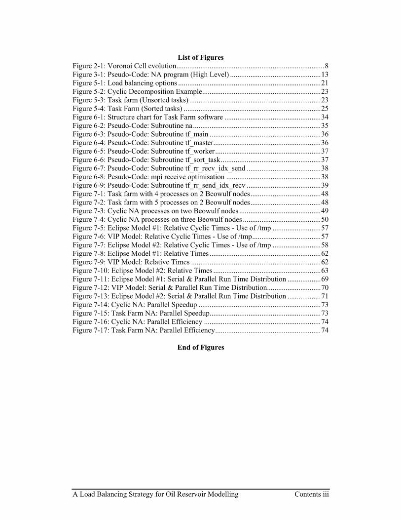
List of Figures
Figure 2-1: Voronoi Cell evolution................................................................................8 Figure 3-1: Pseudo-Code: NA program (High Level) .................................................13 Figure 5-1: Load balancing options .............................................................................21 Figure 5-2: Cyclic Decomposition Example................................................................23 Figure 5-3: Task farm (Unsorted tasks) .......................................................................23 Figure 5-4: Task Farm (Sorted tasks) ..........................................................................25 Figure 6-1: Structure chart for Task Farm software ....................................................34 Figure 6-2: Pseudo-Code: Subroutine na.....................................................................35 Figure 6-3: Pseudo-Code: Subroutine tf_main ............................................................36 Figure 6-4: Pseudo-Code: Subroutine tf_master..........................................................36 Figure 6-5: Pseudo-Code: Subroutine tf_worker.........................................................37 Figure 6-6: Pseudo-Code: Subroutine tf_sort_task......................................................37 Figure 6-7: Pseudo-Code: Subroutine tf_rr_recv_idx_send ........................................38 Figure 6-8: Pesudo-Code: mpi receive optimisation ...................................................38 Figure 6-9: Pseudo-Code: Subroutine tf_rr_send_idx_recv ........................................39 Figure 7-1: Task farm with 4 processes on 2 Beowulf nodes......................................48 Figure 7-2: Task farm with 5 processes on 2 Beowulf nodes......................................48 Figure 7-3: Cyclic NA processes on two Beowulf nodes ............................................49 Figure 7-4: Cyclic NA processes on three Beowulf nodes ..........................................50 Figure 7-5: Eclipse Model #1: Relative Cyclic Times - Use of /tmp ..........................57 Figure 7-6: VIP Model: Relative Cyclic Times - Use of /tmp.....................................57 Figure 7-7: Eclipse Model #2: Relative Cyclic Times - Use of /tmp ..........................58 Figure 7-8: Eclipse Model #1: Relative Times ............................................................62 Figure 7-9: VIP Model: Relative Times ......................................................................62 Figure 7-10: Eclipse Model #2: Relative Times ..........................................................63 Figure 7-11: Eclipse Model #1: Serial & Parallel Run Time Distribution ..................69 Figure 7-12: VIP Model: Serial & Parallel Run Time Distribution.............................70 Figure 7-13: Eclipse Model #2: Serial & Parallel Run Time Distribution ..................71 Figure 7-14: Cyclic NA: Parallel Speedup ..................................................................73 Figure 7-15: Task Farm NA: Parallel Speedup............................................................73 Figure 7-16: Cyclic NA: Parallel Efficiency ...............................................................74 Figure 7-17: Task Farm NA: Parallel Efficiency.........................................................74
End of Figures

_____________________________________________________________________ A Load Balancing Strategy for Oil Reservoir Modelling Acknowledgements
Acknowledgements I would like to thank the many people who have helped me over the course of this
project. My thanks go to Dr. Stephen Booth for his efforts in supervising my work
and particularly for his suggestions regarding some of the more unexpected aspects of
the NA application’s behaviour that were discovered. I am also very grateful to the
project sponsor, Professor Mike Christie, who showed great forbearance in answering
my many questions and in meeting my demands for ever more models to run. The
original NA program author, Malcolm Sambridge, provided welcome expertise during
the code familiarisation phase of the project. My fellow students were very kind in
sharing their Unix knowledge, ideas and suggestions. My thanks also go to Philip
Morris. Any mistakes are my own.
End of Acknowledgements

Introduction Page 1 _____________________________________________________________________
_____________________________________________________________________ A Load Balancing Strategy for Oil Reservoir Modelling
1. Introduction
The Institute of Petroleum Engineering at Heriot-Watt University uses computational
modelling to estimate the properties and likely productivity of oil reservoirs. The
process used requires the generation of large numbers of models derived from varying
sets of input parameters which determine the properties of the resulting model. The
models are sampled to select models which show a good match to observed data and
the selected sample is used as the basis for generating new sets of parameters and
hence new models. This process is repeated for a predefined number of iterations. The
intention is to search out parameter sets that produce a model that closely matches the
observed data.
One the methods of searching the parameter space is the Neighbourhood Algorithm
(NA) [NA1] which searches the available parameter space. The NA program [NA2]
was developed to use this algorithm with a variety of suitable models. The individual
models are computationally independent within each iteration of the process making
them suitable for use with parallel software techniques. The NA program was
converted by from serial Fortran to Fortran and MPI with the aim of reducing the
execution time of the program allowing petroleum scientists to get results on their
desk in a shorter time.
The MPI parallel program assumed that all models had the same execution time and it
was proposed that this was not the case. Variability in model run times would be
likely to result in a load imbalance in the processors running the NA program since it
used a cyclic decomposition; models were allocated to processors in turn regardless of
the model’s individual or aggregate execution times. At the end of each iteration there
is a synchronization point at which all processors must share data. A load imbalance
would result in the processor with the lowest cumulative workload standing idle until
other all processors had completed their fixed number of tasks and reached the
synchronization point. Additionally, if the number of models per iteration was not
exactly divisible by the number of utilised processors then a further imbalance would
arise since some processors would have more models to compute than others.

Introduction Page 2 _____________________________________________________________________
_____________________________________________________________________ A Load Balancing Strategy for Oil Reservoir Modelling
The task farm is a well known decomposition technique that is well suited to load
balancing the execution of computational tasks that have unequal run times. The task
farm achieves a more even load balance by allocating computational work to
processors when they are free to perform work rather than allocating them a fixed
number of tasks regardless of the execution time of the tasks. The task farm approach
to the allocation of NA models to processors was suggested as a potential method of
realizing performance benefits by reducing or eliminating any load imbalance that is
present when the cyclic decomposition is employed. The task farm approach is well
suited since the emphasis of this project is on the scheduling of computational tasks
and not the actual tasks themselves. Many different models can be used within the
framework of the NA program and these models are often in the form of third party
software for which no source code is available. Thus the emphasis is on the
scheduling of tasks and not the tasks themselves.
The NA code base was delivered to EPCC’s Sun cluster (Lomond) for evaluation and
for the implementation of the software modifications required to implement a task
farm. After implementation and initial testing using a dummy problem on Lomond,
the modified code base was ported to a Beowulf Cluster at Heriot-Watt University for
testing with real modelling software. The task farm’s performance was appraised with
a view to determining what, if any, performance improvements had accrued as a result
of the its implementation.
A brief overview of the techniques used for reservoir modelling is given in §2. The
main focus of this report is on the computational science aspects of the application
and not the petroleum science or statistics. Although some discussion of the statistical
modelling methods has been included, any definitions should not be taken as being
rigorous or definitive.
The state of the NA program prior to the start of this project is described in §3. This
includes an outline of the software and hardware environment. The perceived
deficiencies of the original parallel program algorithm that provided the motivation
for this project are also discussed.

Introduction Page 3 _____________________________________________________________________
_____________________________________________________________________ A Load Balancing Strategy for Oil Reservoir Modelling
Some definition and scope is given to the project in §4; this includes project goals and
constraints on possible approaches to the optimisation goals. A number of risks were
identified that might impact on various aspects of the project. These risks are listed
along with the strategies that were adopted to manage them and reduce their potential
impact on the project.
A number of possible optimisation strategies are discussed in §5. This includes
strategies that were chosen for implementation and evaluation as well as those that
were discarded. The motivation for selecting particular strategies is outlined, as are
the reasons for discarding those that were not progressed.
The detailed design of the implemented task farm is shown in §6. The design is
expressed in terms of pseudo code accompanied by a structure chart showing the
hierarchy of the new software modules. The testing and verification techniques
employed to ensure the correctness of the new code are also discussed.
Performance issues are analysed in §7. This includes the methods to be used to
evaluate the performance of the task farm, the effect of enhancements intended to
increase the task farm performance and discussion of observed run times for the
completed task farm. The run times for the task farm are compared with run times for
the cyclically decomposing program to put the task farm performance into context.
§8 attempts to evaluate the impact of the task farm and to draw some conclusions
regarding its effect on computational performance. The implications of some the
findings regarding the performance of the Beowulf cluster at Heriot-Watt are also
talked through. Some recommendations for the project sponsor have been made.
Some suggestions for further work and potentially fruitful new areas of investigation
are outlined in §9. This includes further investigation of some the material covered in
this project. Additionally, it suggests new investigations into some of the issues that
have been discovered during the evolution of this project.
There are also a number of appendices listing references, a summary of the source
code modules, raw data used in graphs and the original project plan.

Introduction Page 4 _____________________________________________________________________
_____________________________________________________________________ A Load Balancing Strategy for Oil Reservoir Modelling
After the new task farm code had been developed and tested using a dummy model it
was tested further using real oil reservoir models. It soon became apparent that there
were performance issues regarding the host platform that were not known at the
beginning of the project. What had initially seemed like a mature and well understood
combination of application software and host hardware turned out to have some quite
poorly understood behaviour and some unexpected characteristics.
As a result of discovering that the application architecture had some significant
performance problems, the project became far more exploratory and investigative
than had originally been intended. These discoveries led to significant digressions
away from the original project plan and the planned activities. Consequently many of
the proposed performance evaluation metrics were judged to be possibly no longer as
informative as was originally hoped. Less time was spent trying to evaluate the
performance of the task farm program across a wide range of problems than had
originally been intended as a result of the time constraints on the project. A significant
amount of unplanned activity was put into identifying the reasons for the host
platform performance problems. This is in turn led to evaluating the impact on and
implications for the computational activities performed on the Beowulf cluster.
The project divided into two streams of activity; implementation and evaluation of the
task farm and understanding the execution environment. The two streams, although
inextricably linked, might be best regarded as two separate projects. If the task farm
evaluation had not been undertaken, the Beowulf cluster performance problems would
not have been identified. Without identification of these problems, their impact on the
parallel codes would have remained undiscovered. Time constraints have limited the
depth and breadth of investigation for both activity streams but despite this much has
been learnt and resulted in an increased level of understanding of both the application
software and its hardware platform.
The situation at the end of the project was that many of the proposed project activities
had not been fully completed. Some activities were not started. However, many of the
unplanned activities have provided a significantly greater understanding into the
behaviour of the Beowulf cluster which will bring future benefits to the planned next

Introduction Page 5 _____________________________________________________________________
_____________________________________________________________________ A Load Balancing Strategy for Oil Reservoir Modelling
generation of hardware to be utilised for computational activities within the Institute
of Petroleum Engineering and also within other parts of Heriot-Watt University.
The project was sponsored by Professor Mike Christie [MC] of the Institute of
Petroleum Engineering at Heriot-Watt University [PE1]. The original developer of the
NA program, Malcolm Sambridge [MS] of the Royal School of Earth Sciences
(RSES), Australia National University, provided assistance during the familiarisation
part of the program and with identifying some of the changes required to the
computational parts of the program.

Basic Concepts of Reservoir Modelling Page 6 _____________________________________________________________________
_____________________________________________________________________ A Load Balancing Strategy for Oil Reservoir Modelling
2. Basic Concepts of Reservoir Modelling
2.1 The Physical Problem
Reservoir modelling is employed in petroleum engineering to try and predict the
properties and future production of an oil reservoir based on available observed data;
the observed data may be small in quantity and not give a detailed representation of
the geology of the oil reservoir. Such observed data might consist of limited
geophysical data concerning the properties of the geological strata in which the oil
reservoir is situated and some limited historic data defining oil and water output from
the reservoir. The amount of geophysical data is limited by the practicalities of
collecting samples from what can be a large volume of geological strata. The
geophysical data might consist of the porosity (the amount of space within the rock
formations) and the permeability (the ease with which fluid can flow through the rock
formations) of the geological strata and other properties which help to define its
behaviour.
Petroleum companies that intend to engage in extractive activities have to make
economic decisions on how to invest in and manage an oil reservoir. To do this, some
estimation of the reservoir’s future value has to be made. Although reservoir
modelling cannot provide an exact prediction of the future output of a reservoir, it can
create predictions that have a probability of accuracy that can be specified. The
predictions can help reduce, but not eliminate, the uncertainty in the decision making
process.
2.2 The Computer Simulation
If numerous computer models are generated from many different sets of input
parameters; each set of input parameters will result in a slightly different model of a
reservoir. The predicted productivity of a generated model can then be compared with
known production data. A close fit between the two productivity curves may indicate
that the set of parameters used to generate the model accurately define the overall
properties of the oil reservoir. To generate a sufficiently large number of models the
various combinations of all possible parameter values must be explored to ensure

Basic Concepts of Reservoir Modelling Page 7 _____________________________________________________________________
_____________________________________________________________________ A Load Balancing Strategy for Oil Reservoir Modelling
completeness and coverage of the sampling. To achieve a thorough exploration of the
parameter space, a number of statistical techniques, such as Monte Carlo Sampling,
Markov Chains, Bayesian Probability [ST1] and Voronoi Cells [VO1] are utilised,
however, very little understanding of these is required to be able to comprehend the
computational modelling activity that takes place within the NA program [NA3]. The
geological modelling software can be regarded as a black box which accepts a set of
parameters and returns a series of simulated values; this is particularly true when the
model consists of third party licensed software with no source code available. The
primary function of the NA program is to search the parameter space to provide
parameter sets for the modelling software. Information regarding these statistical
concepts and their usage within the NA program can be found in more specialised
literature.
At the beginning of an NA program run, the first set of parameters can be optionally
read from an input file. If these are supplied they will be used for generating the first
set of models. Otherwise a set of random points within the parameter space is
generated. Each set of points, whether supplied or generated, is used to create a
reservoir model; this can potentially be many hundreds or thousands of models.
After each model has been generated, it is compared to observed oil production data
and a measure, the misfit, of its difference from the observed data is calculated. The
sets of parameter points that generated the models with the lowest misfit value, that is
those with the closest agreement with the observed production data, are selected as the
starting point for generating the next set of parameter values and hence for the next
set of models to be computed; this process occurs at the end of each iteration. This
requires process synchronization in parallel algorithms as the results from all models
executed by all processes must be available for evaluation and re-selection.
The division of the parameter space is performed using Voronoi Cells. These can be
considered as the volume of parameter space bounded by perpendicular bisectors of
the lines joining a point in parameter space to its nearest neighbours; hence
Neighbourhood Algorithm. A two dimensional example is shown is shown in Figure
2-1 [PE2]. This illustrates the evolution of Voronoi Cells and the sampling points
contained within them.

Basic Concepts of Reservoir Modelling Page 8 _____________________________________________________________________
_____________________________________________________________________ A Load Balancing Strategy for Oil Reservoir Modelling
Figure 2-1: Voronoi Cell evolution
In Figure 2-1(a) there are ten sampled points. The cells have been constructed from
the perpendicular bisectors of the lines joining each point to its nearest neighbours. If
some of these points are re-sampled, then new points will be generated within the
chosen cells and new models generated for these points. When the next parameters are
to be generated the Voronoi Cell boundaries are redrawn to take into account the new
points. As time progresses the number of cells and sampling points increases as seen
in Figure 2-1(b) and (c). The sampling points tend to accumulate in the areas of
lowest misfit and these are indicated by the darker areas of closely packed sampling
shown in Figure 2-1(d). The choice of models with the lowest calculated misfit is
made from all models that have been generated by the program up to this point.
The following notation is used to express some of the numerical values described
above:
nsi Number of initial samples/models
ns Number of samples/models for each subsequent iteration
nr Number of samples/models to be re-sampled
np Number of processors
iter Number of iterations
The total number of models that will be executed in a program run
is )( iternsnsisTotalModel ×+= .

Basic Concepts of Reservoir Modelling Page 9 _____________________________________________________________________
_____________________________________________________________________ A Load Balancing Strategy for Oil Reservoir Modelling
Models that are generated from the nr sampled points in parameter space will be
referred to as having parent cells and parent models. The initial set of models will not
have a parent cell or parent model. On all subsequent iterations the ns models that are
generated will each have a parent cell or parent model which will be one of the nr re-
sampled cells or models.
There are two different approaches that can be used to explore the parameter space
when generating parameter sets to be input to the modelling process. These are
exploration and exploitation. The type of search is determined by the ratio of ns to nr.
The two techniques can be summarised as follows:
Exploration results in a widespread search of the parameter space. An explorative
search is performed when ns and nr are selected to give a lower value of the ratio of
ns/nr; say for example with a value of one or two. A value of one would result in
every one of nr cells being re-sampled once. Each set of parameters would be
subjected to a random walk within its Voronoi cell and then the new set input into the
modelling process. A ratio of ns/nr equal to two would result in the nr cells being re-
sampled twice and two new parameter sets being generated from each of the nr re-
sampled points. Using this approach the sampling points are spread quite widely
through the parameter space.
Exploitation gives a more localised search of the parameter space; it converges more
rapidly on regions of the parameter space producing parameter sets that have given
the lowest misfit results. An exploitative search is performed when ns and nr are
selected to give a higher value ratio of ns/nr, say for example ten. A value of ten
would result in each of the nr cells being used as the starting point for generating ten
new sets of parameters. The number of new sets generated from each point would be
ns/nr.
2.3 Reservoir Models
The behaviour of three models has been investigated. The three models are drawn
from two different types of reservoir model that have different model characteristics

Basic Concepts of Reservoir Modelling Page 10 _____________________________________________________________________
_____________________________________________________________________ A Load Balancing Strategy for Oil Reservoir Modelling
arising from differing termination criteria. The two model types are used are referred
to as “Fixed time” and “Fixed oil”.
• Fixed time: The computational model is run for a fixed period of simulated time.
• Fixed oil: The computational model is run until the oil production falls below a
pre-defined threshold; this is likely to result in the simulated time varying as the
model parameters vary. The simulated oil production will vary over simulated time
as the properties of the parameter driven model vary.
The reservoir modelling is performed by third party licensed packages; sometimes
with additional bespoke software wrapped around the package invocation to create
input data and calculate the resulting misfit of the results returned by the modelling
package. The two modelling packages that have been used are:
• Eclipse … [EC1]
• VIP … [VP1]
The combinations of model types and modelling packages that have been used in this
project are listed in Table 2-1. The reservoir model descriptions were supplied by the
project sponsor [MC3].
Model Type Description Eclipse #1 Fixed time A synthetic model based on an industry benchmark. VIP Fixed time A real example from a Gulf of Mexico [oil] field. Eclipse #2 Fixed oil A modified version of [Eclipse #1] with more
realistic operating conditions.
Table 2-1: Description of Reservoir Models.
The use of three models arose because of a number of discoveries that arose regarding
the behaviour of the execution platform. These discoveries are discussed in detail
later. The motivation for the use of each model was as follows:
Eclipse Model #1: This was the first real model to be run using the task farm. A
number of performance problems were identified when this model was executed. In

Basic Concepts of Reservoir Modelling Page 11 _____________________________________________________________________
_____________________________________________________________________ A Load Balancing Strategy for Oil Reservoir Modelling
addition, the model run times did not exhibit any significant variability as had
originally been expected; the model run times in serial code were mostly in the range
of 14 to 15 seconds. As a result of these it was decided to run the task farm with a
second model in order to compare the performance.
VIP: The VIP model performance was analysed to try and establish whether the
Eclipse model #1 performance problems were the result of the Eclipse package itself
or the result of the size of the model. Also, it was suggested that this model might
have a more variable run times. This was found not to be the case with most models
run in serial code having an execution time very close to 21 seconds.
Eclipse Model #2: This model is the same as Eclipse model #1 but has a different
termination criterion. The “fixed oil” characteristics of this model made it more likely
to have variable run times. Although most models when run in serial code had run
times in the range four to five and a half seconds, the shorter model run time mean
that the variation was more far more significant that for the other two models.

The Existing Architecture Page 12 _____________________________________________________________________
_____________________________________________________________________ A Load Balancing Strategy for Oil Reservoir Modelling
3. The Existing Architecture
3.1 Hardware and Software
The NA program was originally written as a serial program. Each model within each
iteration was executed sequentially, one after the other on one processor. The tasks
(models) that are run by the program are computationally independent from each
other making the program suitable for parallelisation. The parallel version of the
program uses MPI to operate a cyclic distribution of tasks across the available
processors. The NA program is written in Fortran and can be compiled as Fortran 77
or Fortran 90 by means of hash defines included within the source code. The program
can be compiled as a serial program or as a parallel MPI program.
The NA source code was received in early June 2004 from the project sponsor and a
familiarisation exercise was undertaken. The code was also analysed with the aim of
identifying the changes required for the task farm implementation. The code was
loaded onto Lomond to allow some initial runs to take place using a dummy
modelling routine as it was not possible to use the reservoir model software for
licensing reasons.
The algorithm used by the NA program closely follows the process described in §2.2.
The NA program has three major computational parts. These are initialisation,
modelling and bookkeeping. The modelling and bookkeeping parts are executed in an
iterative loop and perform the reservoir modelling, the selection of models with the
lowest misfit and the generation of new sets of parameter values. The algorithm is
shown in high level pseudo code in Figure 3-1 and each part is described in more
detail.

The Existing Architecture Page 13 _____________________________________________________________________
_____________________________________________________________________ A Load Balancing Strategy for Oil Reservoir Modelling
Figure 3-1: Pseudo-Code: NA program (High Level)
Initialisation: Optionally read the initial sample of nsi parameter values or generate a
random sample of points in the parameter space.
Modelling: A series of reservoir models is generated using the set of parameter
values and the misfit of each result is calculated. Initially nsi models are generated
using the nsi parameter sets from the initialisation phase of the program. On
subsequent iterations ns models are generated; nsi can be different from ns.
The modelling is bounded by a barrier in the form of a reduction operation which
results in all misfit values being copied to all processes. The NA program is not tied
to any particular computational model. Suitable modelling software can be easily
integrated with the NA program via one subroutine call and some data configuration.
Bookkeeping: A call to the MPI subroutine MPI_Allreduce acts as a synchronization
point separating the end of the modelling phase from the start of the bookkeeping
phase. Since in the cyclic decomposition different models have been executed on
different processors, the calculated misfit values are also on different processors. The
Begin Program NA Initialisation: Read program configuration data Read nsi initial model data values
For each iteration Modelling: For each model data value Generate forward model Calculate misfit End For [Parallel synchronization point] Bookkeeping: Select nr models with lowest misfit Generate ns new model data values
End For End Program NA

The Existing Architecture Page 14 _____________________________________________________________________
_____________________________________________________________________ A Load Balancing Strategy for Oil Reservoir Modelling
misfit values from each processor are made available to all other processors and then
all processors perform the bookkeeping activities.
The nr parameter value sets that gave the lowest misfit models are then used to
generate the next set of parameter values. Random walks with the Voronoi cell
containing each of the nr parameter values are performed and new parameter values
are determined. The Voronoi Cell boundaries are not calculated but the random walk
used to generate new parameter points is contained within the cell by statistical
means. The number of new parameter sets generated in each of the nr selected cells is
ns/nr.
The new set of ns parameter values is then used as input to the modelling stage. The
modelling and bookkeeping stages are repeated for a user defined number of
iterations. At the end of the process a file containing the parameter sets and their
associated misfit value is output and the parameter set with the lowest misfit value is
identified.
The NA application runs on a Beowulf Cluster at Heriot-Watt University. The cluster
contains thirty two IBM x330 1.26GHz dual processor Pentium III nodes. Each node
has 1.2Gb of memory which is shared between the two CPUs. The computational
nodes are accessed from a front end via a batch job submission system. The job
submission mechanism is OpenPBS V2.3. The operating system used in Linux-Gnu.
3.2 Limitations of the Current Task Scheduling
The current parallel algorithm operates a cyclic decomposition. Tasks are assigned to
each processor in turn until all have been executed. Each processor will execute ns/np
models for each iteration so long as ns is an integer multiple of np. If all tasks
executed in equal times and ns was an integer multiple of np then the cyclic
decomposition would be well load balanced. Up until now it has been assumed that all
tasks execute with the same elapsed time, however, the project sponsor has suggested
that this is not the case. Varying the model parameters or running for different lengths
of simulated time were both believed to result in run times that were variable.

The Existing Architecture Page 15 _____________________________________________________________________
_____________________________________________________________________ A Load Balancing Strategy for Oil Reservoir Modelling
The cyclic decomposition makes no allowance for the length of time taken to execute
a task. Each processor is assigned a fixed number of tasks regardless of the length of
time that they take to execute. Since there is a synchronization point after each
iteration of modelling the processor that is last to complete its assigned tasks will
create a constraint on the minimum run time for the iteration. While the processor
with the longest cumulative run time is finishing its allotted tasks, the other processors
will be waiting, idle, at the synchronization point for the last processor to catch up.
The project sponsor had calculated the parallel efficiency of the cyclic NA program to
be in the region of 70%. It was hoped that the task farm implementation would be
able to improve on this figure resulting in shorter program execution times.
A second source of load imbalance for the cyclic program would arise if ns is not an
integer multiple of np; some processors will have to execute one more task than other
processors. The can be avoided by careful selection of the value of ns which does not
have to be a precise value to meet the requirements of the petroleum science.

Project Definition Page 16 _____________________________________________________________________
_____________________________________________________________________ A Load Balancing Strategy for Oil Reservoir Modelling
4. Project Definition
4.1 Project Goals
To achieve 95% parallel efficiency: This is an arbitrary figure chosen to give a
target for the hoped for performance improvement.
To verify the results of the new code as being correct: It is clearly important that
the results from the modified program can be verified as correct against results from
the existing program.
To reduce the overall program run time: The object of the project is to reduce the
execution time for any series of reservoir models that is generated by the NA program
by means of better computational load balancing.
To understanding the reasons for any performance improvement: In addition to
reducing the execution time of the application it is hoped to be able to identify the
sources and causes of the reductions in execution time.
4.2 Project Deliverables
Report: This report is the primary deliverable.
Software: Amended program code that will satisfy the project goals of producing
verifiable results within a shorter period of elapsed time than is currently possible.
4.3 Project Constraints
The existing program search algorithm cannot be changed: The focus of this
project is on computational science and not petroleum science. To attempt changes to
the program’s search algorithm would be unfeasible as it lies outside the student’s
area of expertise and additionally would not be achievable within the project
timescales.

Project Definition Page 17 _____________________________________________________________________
_____________________________________________________________________ A Load Balancing Strategy for Oil Reservoir Modelling
The reservoir modelling code cannot be changed: The modelling software that
constitutes the computational tasks that require load balancing cannot be changed as it
is third party licensed software; the source code is not available.
The project has fixed timescales: Software development and analysis has to be
completed by a fixed and unmoveable deadline. It is important that the project has
clearly defined goals and that these goals are achievable.
4.4 Project Plan
Detailed planning at the start of the project was difficult because of the lack of
familiarity with the application code. Ideas and hence direction were expected to
clarify as the project progressed and a forward path became more apparent. A
provisional project plan is shown in Table 4-1. A detailed plan was produced after the
initial phase of familiarisation and analysis (§13).
Duration Activities Intended Outcome June • Familiarisation.
• 8th June 2004 - Student presentations.
• Evaluate current performance. • Formulate ideas for performance
improvement. • Produce detailed project plan.
• Familiarity with the NA application • Completed presentation. • Some knowledge of the NA
applications current performance. • Ideas with which to progress the
project. • A detailed project plan. (See §13).
July • Design and implement modifications.
• Verify correctness of modified code.
• Determine methods of performance evaluation.
• Software design and completed code. • Debugged code that functions
correctly and as intended. • Metrics to quantify the new code
performance.
Aug (1st half) Evaluate performance of new code. A good understanding of how well the new code performs measured using pre-defined metrics.
Aug (2nd half) – September
Writing up. A completed project report.
10th September Hand in completed code and completed report.
Project completion
Table 4-1: Provisional project plan.

Project Definition Page 18 _____________________________________________________________________
_____________________________________________________________________ A Load Balancing Strategy for Oil Reservoir Modelling
4.5 Project Risks and Management
There are a number of risks associated with this project. These are listed in Table 4-2
along with the proposed method of management where management is possible. A
qualitative assessment of the likelihood (Lik) and impact (Imp) of each risk has been
given in terms of low (L), medium (M), high (H) and fatal (F). Owing to the
investigative nature of many aspects of the project it was not believed that a
quantitative assessment of the impact of risks would have sufficient accuracy to be
meaningful. Although the impact of many of the risks is high, the likelihood of
occurrence is in most cases low. Many of the risks can be managed thus reducing their
likelihood of having a negative impact on the project. Given that the impact of the
risks on the project is not readily quantifiable the project will be regarded as medium
to high risk.
Risk Management strategy Lik Imp
1 Risk Risks: • The risk analysis may not be
accurate because of the lack of experience with the application.
• The risk analysis may not be
accurate because of unforeseen events occurring.
• Carry: This is unavoidable given that the
project is investigative and, by its very nature, has an element of uncertainty attached to it. The risk will have to be carried.
• The risk level associated with this project will be considered as medium to high.
• This risk should be borne in mind when considering all project risks.
M
M
M
M
2 Personnel Risks: • Lack of understanding. • Poor progress. Invalid conclusions. • Attempting over ambitious
goals.
• Manage: Consult with project supervisor
and project sponsor. • Manage: Regular meetings with
dissertation supervisor to review material deliverables and discuss any project issues arising.
• Manage: Assess each activity for achievability. Ensure that activities can be realistically achieved in the time available.
M
M
L
H
H
M

Project Definition Page 19 _____________________________________________________________________
_____________________________________________________________________ A Load Balancing Strategy for Oil Reservoir Modelling
Risk Management strategy Lik Imp3 Implementation Risks:
• Lack of time. • Lack of detailed plans. • Unavailability of development
facilities. • Loss of modified source code.
• Manage: Produce a project plan (see
§13) and adhere to it. • Manage: The lack of a detailed plan
owing to the investigative nature of the early stages of the project carries the risk of slippage owing to unforeseen exigencies arising. A more detailed plan can be produced after the period of familiarisation and analysis.
• Carry: Will delay development activities.
• Avoid: Use RCS for version control of source code.
L
L
M
L
H
H
H
H
4 Performance Risks: • Lack of ideas. • Lack of successful ideas. • Lack of performance
improvement.
• Carry: It may be the case that no ideas
arise as to how to improve performance. • Carry: It has to be accepted that there
may not be viable improvements that can be implemented; this does not detract from the merit of the project.
• Carry: Accept that performance improvement may not be possible. If the project goal figure of 95% parallel efficiency is not achieved the project is not a failure. The figure was arbitrarily chosen to provide a target. Any performance increase can be regarded as successful. Determining why no performance improvements are possible is still a valid outcome.
M
M
M
M
L
L
5 Quality Risks: • Delivery of poor quality
software. • Delivery of a poor quality
report.
• Manage: Ensure that software is well
designed, carefully coded and tested and then reviewed.
• Manage: Review report contents with supervisor. Revisit MSc coursework feedback to identify strengths and weaknesses.
L
L
H
H
6 Deliverables and Deadline Risks: • Failure to complete project
hand-in. • Failure to meet 10th September
deadline.
• Manage: This is not an option
L
L
F
F
Table 4-2: Risk Management Strategy

Approaches to Improving Parallel Efficiency Page 20 _____________________________________________________________________
_____________________________________________________________________ A Load Balancing Strategy for Oil Reservoir Modelling
5. Approaches to Improving Parallel Efficiency
5.1 Task Scheduling Options
To achieve high parallel efficiency it is essential to ensure that each processor
performs equal amounts of work. The shortest run time will be constrained by the
longest cumulative execution time of any processor. When running ns reservoir
models on np processors the approximate loading of each processor will be ns/np
models. A number of options were examined for improving the load balance on each
processor; the options varied according to the value of ns/np. The chosen method for
improving load balance was by means of implementing a task farm to replace the
current cyclic decomposition. The task scheduling options were also considered in
conjunction with task ordering options (see §5.2). The decisions used in arriving at
the options are illustrated in Figure 5-1 and are explained in detail below.
• ns < np: Using ns < np is not recommended by the application developer as it is
wasteful of computational resources. Running under these conditions will result in
(np – ns) processors being idle and unavailable to other users.
• ns = np: If application usage was restricted to ns = np then no performance
improvement would be possible using the existing program algorithm. Since only
one task is executing on each processor, it would not be possible to implement load
balancing by means of a task farm approach as there would no scope for allocating
tasks across different processes. Since utilisation of the existing program algorithm
is a project constraint (§4.3), a new algorithm cannot be adopted for this project.
The focus of this project is task scheduling and devising new algorithms would be
well outside the scope of the project.
• ns ≈ np: Sorting the tasks by descending execution time (with or without the task
farm approach) might bring benefits by allowing the longest running tasks to
complete first. This approach requires the existence of a reliable method of
predicting the execution time of a computational task.

Approaches to Improving Parallel Efficiency Page 21 _____________________________________________________________________
_____________________________________________________________________ A Load Balancing Strategy for Oil Reservoir Modelling
Figure 5-1: Load balancing options
Implement a new method of selecting each newmember of nr individually as a job completes.The existing algorithm of batching ns jobswould have to be changed.
Existing algorithm
New algorithm
ns < np
ns = np
ns ≈ np
ns >> np
ns >>> np
Implement a task farm. Attempt to sort tasks sothat largest/longest begins first. Would dependon being able to determine model run timefrom the model parameters or estimate it fromthe run times of the nr re-sampled models.
Implement a task farm with dynamicdecomposition. Processors receive tasks on afirst come first served basis to achieve loadbalance. Optionally combine with taskordering.
A cyclic decomposition as done currentlymight naturally load balance for a large enoughnumber of jobs per processor. However, a taskfarm with or without task ordering should notmake the performance any worse and mayimprove the performance.
Should not be (and is not) used. Moreprocessors than models results in the wastedallocation of idle processors.
Yes
Yes
Yes
Yes
Yes
No
No
No
No
ns = number of models np = number of processors nr = number of re-sampled models
Approaches to Improving Parallel Efficiency Page 22 _____________________________________________________________________
_____________________________________________________________________ A Load Balancing Strategy for Oil Reservoir Modelling
• ns >> np: A task farm with dynamic decomposition should aid load balancing by
allowing tasks to be processed by the first available processor. Again, ordering
tasks by descending execution time should improve the load balancing.
• ns >>> np: For very high values of ns/np, the application may naturally load
balance because of the effects of the “law” of large numbers. A large enough
number of varying run times may average itself across the available processors. A
task farm, again with task ordering, would be likely to improve performance
further by improving the load balance across processors. It does not seem likely
that a task farm would make performance any worse.
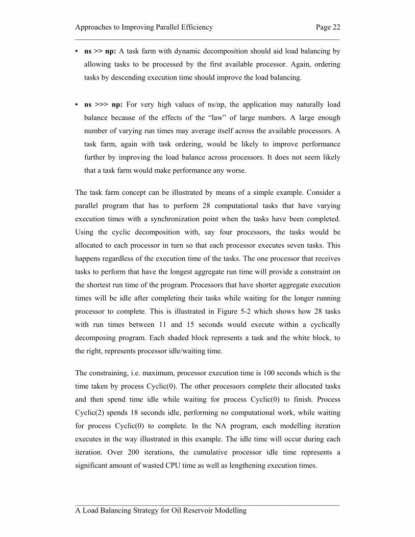
The task farm concept can be illustrated by means of a simple example. Consider a
parallel program that has to perform 28 computational tasks that have varying
execution times with a synchronization point when the tasks have been completed.
Using the cyclic decomposition with, say four processors, the tasks would be
allocated to each processor in turn so that each processor executes seven tasks. This
happens regardless of the execution time of the tasks. The one processor that receives
tasks to perform that have the longest aggregate run time will provide a constraint on
the shortest run time of the program. Processors that have shorter aggregate execution
times will be idle after completing their tasks while waiting for the longer running
processor to complete. This is illustrated in Figure 5-2 which shows how 28 tasks
with run times between 11 and 15 seconds would execute within a cyclically
decomposing program. Each shaded block represents a task and the white block, to
the right, represents processor idle/waiting time.
The constraining, i.e. maximum, processor execution time is 100 seconds which is the
time taken by process Cyclic(0). The other processors complete their allocated tasks
and then spend time idle while waiting for process Cyclic(0) to finish. Process
Cyclic(2) spends 18 seconds idle, performing no computational work, while waiting
for process Cyclic(0) to complete. In the NA program, each modelling iteration
executes in the way illustrated in this example. The idle time will occur during each
iteration. Over 200 iterations, the cumulative processor idle time represents a
significant amount of wasted CPU time as well as lengthening execution times.

Approaches to Improving Parallel Efficiency Page 23 _____________________________________________________________________
_____________________________________________________________________ A Load Balancing Strategy for Oil Reservoir Modelling
Cyclic Task Execution (100s)
0 25 50 75 100
Cyclic(0)
Cyclic(1)
Cyclic(2)
Cyclic(3)C
yclic
Pro
cess
Time (s)
Figure 5-2: Cyclic Decomposition Example
The task farm approach is intended to reduce the processor idle time by allocating
tasks to processors when they are ready to do work rather than on a turn by turn basis.
The first come first served approach gives work to processors when they are ready to
work rather than making a processor wait its turn. The result of taking the same 28
tasks shown in the cyclically decomposing example and distributing them to
processors using the task farm method is shown in Figure 5-3. The master process,
process (0), which does not execute any modelling tasks, is not shown.
Task farm Unsorted Task Execution (91s)
0 25 50 75 100
Worker(1)
Worker(2)
Worker(3)
Worker(4)
Task
Far
m P
roce
ss
Time (s)
Figure 5-3: Task farm (Unsorted tasks)

Approaches to Improving Parallel Efficiency Page 24 _____________________________________________________________________
_____________________________________________________________________ A Load Balancing Strategy for Oil Reservoir Modelling
Using the task farm approach has had two significant effects. Firstly, the time spent
idle by any processor has been significantly reduced; the maximum processor idle
time on Worker(4) is four seconds. Secondly, the overall execution time has been
reduced to 91 seconds; a reduction of nearly 10%. If the example tasks were
performed over 200 iterations using the task farm then the end result would be to
reduce the run time from approximately five and one half hours, for the cyclic
decomposition, to about five hours for the task farm. Given enough tasks with enough
variation in run times it is possible for individual task farm processes to execute
different numbers of tasks to achieve the load balance.
The cyclic and task farm examples are both somewhat simplified. In reality the
performance will be slightly different from that which has been illustrated. The
overall timings make no allowance for inter-process communication which will
slightly increase the overall run time for the task farm. When allocating tasks, the task
farm master process has to receive a message indicating that the worker process is
ready to perform computational work. The master process will then send a task
identifier to the worker process for execution. Until the task identifier has been
received by the worker process it cannot begin execution of the task. If the time for
communications to complete becomes significant then it could reduce the
effectiveness of the task farm performance.
5.2 Task Ordering Options
In addition to considering the scheduling of reservoir models some ideas for
improving the load balance by ordering the computational tasks were also proposed.
The task farm approach would gain additional benefit from ordering the tasks by
descending execution time. The benefit arises from executing the longest running
tasks first and avoiding a situation where the last task to be executed is the longest.
This could cause an imbalance in the work performed by each processor resulting in
processors spending time idle. If the last task to be performed has the shortest
execution time the maximum potential processor idle time is reduced by the
difference of the longest and shortest task run times. If the same 28 tasks used in §5.1
are ordered by descending execution time and then allocated to processors for
execution in this order then a small reduction in run time can be observed and the

Approaches to Improving Parallel Efficiency Page 25 _____________________________________________________________________
_____________________________________________________________________ A Load Balancing Strategy for Oil Reservoir Modelling
amount of processor idle time is reduced. The overall run time is slightly reduced to
90 seconds and the maximum processor idle time is one second. Over 200 iterations,
the reduction in run time would be about three minutes. This is illustrated in Figure
5-4. As before, this is an idealised figure; no attempt has been made to model inter-
processor communications which may slightly reduce the effectiveness of the task
farm.
Task farm Sorted Task Execution (90s)
0 25 50 75 100
Worker(1)
Worker(2)
Worker(3)
Worker(4)
Task
Far
m P
roce
ss
Time (s)
Figure 5-4: Task Farm (Sorted tasks)
The proposals were dependent on the ability to predict the relative execution time of a
model. Two potential methods that were proposed were:
• Finding a heuristic that would allow tasks to be sorted by expected relative
execution time. Two possibilities are:
Assume that the run time of the parent model in nr used to generate new points in
ns is representative of the expected run time of the new model.
Interpolate between the nearest known points in parameter space from last set of
ns times to determine the expected run time of the next model.
• Finding some correlation between model parameters and model execution time:

Approaches to Improving Parallel Efficiency Page 26 _____________________________________________________________________
_____________________________________________________________________ A Load Balancing Strategy for Oil Reservoir Modelling
Existence of some correlation between model parameters (e.g. porosity,
permeability) and model execution time that would allow tasks to be ordered by
predicted model execution time.
In the event of no algorithm being determined and there being no known correlation
between model’s parameters and model execution time it would not be possible to
perform task ordering using the latter proposal. On advice from the project sponsor,
this turned out to be the case and this proposal was dropped in favour of the heuristic
approach.
For reasons of simplicity of implementation, the first suggested heuristic was chosen.
It was to be assumed that the predicted execution times of a series of models could be
ordered according to the execution time of the model from the parent cell. This
hypothesis would then be tested and its accuracy quantified by observation and
analysis of run time data. The method to be used to determine the effectiveness of the
heuristic is discussed in §7.3. It should be emphasised that the chosen heuristic is
entirely intuitive and is not based on any understanding of the operation of the
modelling packages or of the underlying geological/petroleum science.
The sorting algorithm will be affected by the values of ns and nr. When nr cells are re-
sampled, ns/nr new parameter sets will be generated in each of the nr cells. Each of
the new ns models will have a predicted time based on the actual time of the one
model out of nr models. The predicted times will be in groups of ns/nr. To take a
simple example, consider ns=20 and nr=4. Each of the four re-sampled models will be
used to predict the execution time of five models. Five models will be predicted to be
slowest, based on the slowest of the nr re-sampled models, followed by another three
groups of five models each of which will have successively faster predicted run times.
5.3 Code Re-Engineering
Extensive work on the computational parts of the application code could potentially
yield some performance improvement if the calculations could be parallelised. It was
decided not to pursue this option for a number of reasons. Much of the computational
modelling code is licensed and hence no source code is available. Any components of

Approaches to Improving Parallel Efficiency Page 27 _____________________________________________________________________
_____________________________________________________________________ A Load Balancing Strategy for Oil Reservoir Modelling
the modelling software that have source code available would be sufficiently complex
to make parallelising it a project in its own right.
The bookkeeping part of the NA algorithm is performed on all processors. This
activity has to be completed before the next iteration can proceed. In theory, the
bookkeeping needs only be performed on one process and not replicated on all
processes. There would be little or no benefit in re-engineering the code to achieve
this. The bookkeeping is a minor component of the overall run time and its duration
would not be reduced by running on one process only.
General code re-engineering that was not directly related to the new scheduling
regime of the task farm would violate design imperative 7 (see §6.1). The focus of
this project is on the task scheduling which requires macro level changes rather than
the examination of every line of code to try and identify micro level optimisations.
5.4 Compiler Optimisations
The potential for improving performance by selection of appropriate compiler options
was briefly investigated. The compiler used for building software on the Beowulf
cluster is the Portland Group Fortran 90 (PGF) compiler [PG1]. As will be discussed
later, the impact of any compiler optimisations on the performance of the NA program
would have little effect on the overall application execution time. The compiled
components and script language procedures of an NA program run take up a minor
part of the total execution time. The major part of the execution time is taken up by
third party licensed modelling packages for which the source code is not available and
hence cannot be optimised. It was, however, though worthwhile to check for any
suitable compiler options as they are often a safe, quick and reliable way of improving
code performance. The following options were checked for suitability:
Compiler optimisation using –fast: Used by default for existing and new code.
Bounds checking: Not used by default for existing and new code.

Approaches to Improving Parallel Efficiency Page 28 _____________________________________________________________________
_____________________________________________________________________ A Load Balancing Strategy for Oil Reservoir Modelling
Processor specific optimisation “–tp p6”: The PGF compiler User Guide states that
the compiler automatically optimises for the host processor by default [PG1]. A target
processor (tp) can be specified as a command line option when running the compiler.
The compiler option “–tp p6” is intended to optimise for the Intel Pentium III
processor; this is the processor used in the Heriot-Watt Beowulf cluster. When the
compiler option “–tp p6” was specified, the resulting executable program had longer
execution times than when it was not used. The “–tp p6” compiler option was not
used; no further investigation into its behaviour was undertaken.

Software Modifications Page 29 _____________________________________________________________________
_____________________________________________________________________ A Load Balancing Strategy for Oil Reservoir Modelling
6. Software Modifications
6.1 Design Imperatives
The limited timescales and the fixed delivery date for the project were the driving
force behind the decision to specify a number of imperatives for the work to be
carried out. These were intended to ensure that the delivered software contained
working functionality for the highest priority tasks. It was felt preferable to deliver a
completed sub-set of the required functionality with sign posts for future work rather
than aim to deliver a full set of functions but for them to be incomplete on project
delivery date. The design imperatives are listed below:
1 Simplify the source code: The code contained hash defines for Fortran 77
compatibility (serial compilation) and for a toolkit used by the program author.
This code was removed to simplify the development phase of the project; the
extra code was visual clutter for this project and was not needed for the task
farm development. The baseline code consisted of the MPI implementation
only; removal of the serial code and toolkit gave a clean and readable baseline
from which to start task farm development. The aim of the project was to
demonstrate the viability, or otherwise, of the task farm concept which is
inherently parallel and for which no serial code version would be possible.
Thus the serial code was considered redundant. If time allowed at the end of
the project, it was planned to undertake a refactoring exercise to integrate the
task farm functionality into the full source code. The project sponsor advised
that none of this excised code would be needed in their future development
plans and hence it was not given any further consideration [MC1].
2 Encapsulate new functionality: All new functionality should, where
possible, be contained within new subroutines so as to avoid intrusive changes
to the existing code. This also reduces the chances of introducing errors to
existing functionality.

Software Modifications Page 30 _____________________________________________________________________
_____________________________________________________________________ A Load Balancing Strategy for Oil Reservoir Modelling
3 No cosmetic source code changes: No attempt would be made to tidy or
improve the existing code except when it was to be modified to implement
task farm functionality. This imperative precludes activities such as
reformatting code and making cosmetic alterations with the intention of
beautifying the code. In addition to bringing no performance benefits, making
cosmetic changes carries the danger of introducing source code errors and
hence invalid results.
4 Modifications to existing code to match the existing style: Source code
changes to existing code will be implemented in the style of the existing code
but will be clearly highlighted as being new or changed code.
5 New routines in programmers preferred style: New subroutines will be
written in this programmers preferred style.
6 Phased implementation: Having decided upon a set of tasks for the
implementation and prioritised them, each task would be commenced only if
there was sufficient time to design, to code and to test the necessary changes.
Tasks would not be started if there was insufficient time to complete them to a
satisfactory standard.
7 No extensive re-engineering: The main focus of the project will be on re-
working the lines of code that distribute the tasks across the processors.
Within the remainder of the code there are undoubtedly opportunities for
improving the performance. However, given the time available it would not be
feasible to restructure the whole program. Concentrating on the distribution of
tasks will hopefully prove the case for the task farm.
6.2 Implementation Goals
Having been able to evaluate the NA software it was possible to decide in broad terms
how the task farm should be implemented. In conjunction with the design imperatives,
this gave rise to a number of readily identifiable tasks that would be necessary. This
exercise was performed at the earliest opportunity to lessen the project risk caused by

Software Modifications Page 31 _____________________________________________________________________
_____________________________________________________________________ A Load Balancing Strategy for Oil Reservoir Modelling
the lack of a detailed project plan at the beginning of the project. The goals have been
divided into two groups; high priority tasks which it was hoped would all be
completed and lower priority goals which would be completed if deadlines and
timescales permitted. The prioritised implementation goals are listed in §6.2.1 and
§6.2.2 as well as being shown in the project plan in §13.
6.2.1 Highest Priority Goals
1 Code preparation: Create a baseline for the new task farm development in
accordance with design imperative 1.
2 Code repository: Create directories for a copy of the existing code (for
reference) and for the baseline for the new code (for development). Each
directory to have an RCS source code library for version control and software
management.
3 Design Methodology: Particular attention was given to the selection of a
suitable design methodology and development model. The waterfall
development model was chosen for the design, implementation and testing of
the task farm software. Having decided on the task farm option, the
development is hoped to be straight forward. Once testing and evaluation
begins there may be some small scale evolutionary iterative loops involving a
re-work and re-test cycle, however, it is believed that the main development
can be achieved using a simple waterfall model.
4 Draft design: Produce an initial design for the task farm software and
maintain it in the light of any design changes that occur during implementation
of the code (see §6.3).
5 Implement basic task farm: Write the task farm code, review and rework as
necessary. Each reservoir model requires a user_init routine to define the
parameter ranges and a bespoke forward routine. The user_init routines are
supplied by the project sponsor. The forward routines are small and will be
developed as required with support from the project sponsor.

Software Modifications Page 32 _____________________________________________________________________
_____________________________________________________________________ A Load Balancing Strategy for Oil Reservoir Modelling
6 Devise task sorting algorithm: Determine an algorithm for sorting task by
descending estimated run time. The estimated run time of a task is being
determined by assuming that the run time of a model from the parent cell is
representative of the predicted derivative model run time.
7 Implement task sorting algorithm: Write the task sorting code, review and
rework as necessary.
8 Verify correctness using simple models: Verify the correctness of the task
farm by comparing results with those produced by the existing program.
9 Port code from Lomond to Heriot Watt Beowulf cluster: Having developed
the basic task farm functionality on Lomond, the code would require porting
to its intended destination environment. This may require minor tailoring of
the software to ensure compatibility with the different environment.
10 Verify correctness using real model(s): Verify the correctness of the task
farm out by comparing results with those produced by the existing program.
11 Complete dissertation report: Complete the major part of the dissertation
report.
6.2.2 Lower Priority Goals
1 Retain existing cyclic decomposition functionality: It is hoped to be able to
retain the existing cyclic decomposition functionality within the new task farm
code so that it can be optionally executed. If completion of this goal will have
any significant impact on the completion of higher priority goals then it will
be dropped.
2 Refactor NA code base: The task farm functionality will be merged back into
the original code base if time permits.

Software Modifications Page 33 _____________________________________________________________________
_____________________________________________________________________ A Load Balancing Strategy for Oil Reservoir Modelling
6.3 Detailed Design
6.3.1 Task farm description The concept of a task farm is well known and its use in parallel computing for load
balancing the execution of independent tasks is quite widespread. A controlling
(master) process allocates tasks to subordinate (worker) processes; each worker
process requests a new task when it becomes free. The load balancing is achieved by
giving a worker more work when it is ready whereas the cyclic decomposition will
give a fixed number of tasks to each process regardless of their execution time. Since
a synchronization point follows the execution of the tasks, the cyclic decomposition
will have to wait for the slowest process to finish and this will force a constraint on
the shortest possible run time. The task farm will also have to synchronize after task
execution but will potentially shorten the wait for the slowest process by distributing
the required computation more evenly across the worker processes.
In terms of software, both master and worker processes execute the same program but
will follow different paths through the code depending on their status. The master
process will execute a controlling subroutine that allocates tasks to worker processes.
The worker processes will execute a subroutine that requests a task to perform and
then execute the task that it has been allocated. A structure chart for the task farm
routines is shown in Figure 6-1 and the functions are described in detail in §6.3.2.
The master process performs little or no computation during the task execution phase.
To dedicate a whole processor for the exclusive use of the master process would be
wasteful of resources. The master process will share its processor with a worker
process. Although the two processes will potentially be competing for CPU time, the
master process can spent much of its time swapped out. The use of a sleep function to
avoid a busy wait state when the master process is waiting to receive messages will
further reduce the time that it spends active. The implementation of the sleep state is
described in the next section.

Software Modifications Page 34 _____________________________________________________________________
_____________________________________________________________________ A Load Balancing Strategy for Oil Reservoir Modelling
Figure 6-1: Structure chart for Task Farm software
6.3.2 Pseudo-code of new software New software developed for the task farm implementation and modifications to
existing code are specified below. Each new subroutine is outlined using high level
pseudo-code to define its major functions.
subroutine na: This existing subroutine controls the whole program’s execution. It
has been modified to execute the task farm or the existing cyclic decomposition
according to a run time option specified by the user. Outside of the main iterative
modelling loop the subroutine functionality is largely unchanged. Small localised
modifications have been made to accumulate timing information and parent
model/cell information. The subroutine also executes an installation script to create
file structures necessary for execution of the modelling packages.
Main program (subroutine NA – main controlling
routine)
cyclic_decomp (Existing functionality: call
routine to run forward model)
tf_main (Task farm controller)
tf_master (Task farm master – hand out
tasks to task farm worker)
tf_worker (Task farm worker – execute tasks
assigned by task farm master)
tf_rr_recv_idx_send(Receive a ready request from a
task farm worker and send a task)
tf_rr_send_idx_recv(Send a ready request to the task farm master and receive a task)
tf_def_mpi (Define MPI data structures)
tf_task_sort (Sort the tasks by
descending execution time)
forward (Run the forward model &
calculate misfit)

Software Modifications Page 35 _____________________________________________________________________
_____________________________________________________________________ A Load Balancing Strategy for Oil Reservoir Modelling
Figure 6-2: Pseudo-Code: Subroutine na
subroutine cyclic_decomp: Perform the cyclic decomposition from the original
program; this code is unchanged other than being separated off into a new subroutine.
subroutine tf_def_mpi: Define the MPI data types used by the task farm. There
are two MPI data types created for use by the task farm. They are used for the
contents of the messages sent between the master and worker processes. The two MPI
data types are described below.
• mpi_myid: Sent by worker process to master process. Contains the process id of
the worker process indicating that the worker is ready to receive a task to execute.
The data type contains one integer.
• mpi_idx: Sent by master process to worker process. Contains an index into the
array of parameters that are passed to the forward model and an index into the
array of misfit values where the calculated misfit value is to be stored. The data
type contains two integers.
subroutine tf_main: This is the task farm controlling routine. The root process acts
as the task farm master process and allocates tasks to worker processes. Non-root
processes become worker processes. The identity of the root process is specified as a
run time option.
Begin subroutine na ... Existing code ... Execute installation script.
If ( User execution option = Cyclic ) then execute cyclic decomposition … (cyclic_decomp) else if ( User execution option = Task Farm ) then define mpi data structures … (tf_def_mpi) execute task farm … (tf_main) Endif ... Existing code ...
End subroutine na

Software Modifications Page 36 _____________________________________________________________________
_____________________________________________________________________ A Load Balancing Strategy for Oil Reservoir Modelling
Figure 6-3: Pseudo-Code: Subroutine tf_main
subroutine tf_master: The master process generates model and misfit indices that
specify the location within arrays of model and misfit data. If task sorting has been
requested then the tasks will be sorted according to their descending predicted
execution time. The master process receives a “ready to work message” from a
worker process. On receipt of such a message, the master process despatches a model
number to the worker processes. The model number is an index into an array of model
parameters which is present on each process. When all modelling tasks have been
despatched to worker processes, the master process will send a “no more tasks”
message to each worker process so that the worker knows to terminate task
processing. The master process then exits this subroutine.
Figure 6-4: Pseudo-Code: Subroutine tf_master
Begin subroutine tf_main
If ( MPI process id = User specified root ) then Function as task farm master process …(tf_master) else Function as task farm worker process …(tf_worker) Endif
End subroutine tf_main
Begin subroutine tf_master
Generate model parameter indices Generate misfit indices If ( not first iteration and sorting is enabled ) then Sort models by parent run time …(tf_task_sort) Endif For each model Wait for worker ready request …(tf_rr_recv_idx_send) ( Receive worker process id & Send model and misfit indices ) End for For each worker process Wait for worker ready request …(tf_rr_recv_idx_send) ( Receive worker process id & Send end-of-models and end-of-misfits ) End for
End subroutine tf_master

Software Modifications Page 37 _____________________________________________________________________
_____________________________________________________________________ A Load Balancing Strategy for Oil Reservoir Modelling
subroutine tf_worker: The worker process sends a “ready to work” message to the
master process. After despatching this message the worker waits to receive a model
number which indicates the task that it is to perform. On completion of the allocated
task, the worker process stores the misfit value and requests another task. This
continues until the worker process receives a “no more tasks” message instead of a
model number. On receipt of this message, the worker process exits this subroutine.
Figure 6-5: Pseudo-Code: Subroutine tf_worker
subroutine tf_task_sort: The sorting routine sorts the tasks to be executed into
descending estimated execution time. The estimated execution time is that of the
parent cell from which the model parameter set was derived. The subroutine uses a
working copy of the array of parent cell execution times and locates the longest time
down to the quickest and sorts the next set of tasks to be executed according to this.
Figure 6-6: Pseudo-Code: Subroutine tf_sort_task
Begin subroutine tf_worker
While ( not end-of-models & not end-of-misfits ) Send ready request to master …(tf_rr_send_idx_recv) ( Send workers own process id & Receive model and misfit indices )
If ( not end-of-models & not end-of-misfits ) then Execute forward model …(forward) Endif
End while
End subroutine tf_worker
Begin subroutine tf_task_sort
For each task [i] Bigloc = index of maximun Parent_run_time …(maxloc) Model_index_sorted[i] = Models_index_orig[Bigloc] Misfit_index_sorted[i]= Misfit_index_orig[Bigloc] Parent_run_time[Bigloc]=0.0 End For
End subroutine tf_task_sort

Software Modifications Page 38 _____________________________________________________________________
_____________________________________________________________________ A Load Balancing Strategy for Oil Reservoir Modelling
subroutine tf_rr_recv_idx_send: This subroutine is called by the master process
when it is ready to receive a request from a worker process indicating that the worker
is ready to process a task. On receiving a worker request, the master sends indices into
the array of model parameters that the worker is to read and also into the array of
misfit values where the worker will write the misfit value that it has calculated.
Figure 6-7: Pseudo-Code: Subroutine tf_rr_recv_idx_send
When developing the task farm on Lomond, a further refinement was added to this
subroutine to reduce CPU usage arising from a busy wait state when the MPI message
receive subroutine was waiting for a message from a worker process. The master
process can check for waiting messages using MPI_Iprobe. If no messages are
waiting then the master process can be suspended using a call to the sleep
subroutine. The sleep routine takes an integer value of seconds and cannot be tuned
more finely than this. The behaviour of this functionality on the Heriot-Watt Beowulf
cluster is discussed in §7.4. The call to MPI_Recv was replaced with the following
algorithm:
Figure 6-8: Pesudo-Code: mpi receive optimisation
Begin subroutine tf_rr_recv_idx_send
Receive worker id …(mpi_recv) Send model index & misfit index to worker process …(mpi_send)
End subroutine tf_rr_recv_idx_send
... Existing code ... message waiting = .false. Do while ( .not. message waiting )
check for waiting messages …(mpi_probe) ( Returns message waiting = true or false ) If ( .not. message waiting ) then suspend master process …(sleep) Endif End do Receive worker id …(mpi_recv) ... Existing code ...
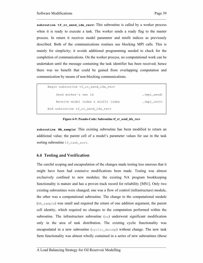
Software Modifications Page 39 _____________________________________________________________________
_____________________________________________________________________ A Load Balancing Strategy for Oil Reservoir Modelling
subroutine tf_rr_send_idx_recv: This subroutine is called by a worker process
when it is ready to execute a task. The worker sends a ready flag to the master
process. In return it receives model parameter and misfit indices as previously
described. Both of the communications routines use blocking MPI calls. This is
mainly for simplicity; it avoids additional programming needed to check for the
completion of communications. On the worker process, no computational work can be
undertaken until the message containing the task identifier has been received; hence
there was no benefit that could be gained from overlapping computation and
communication by means of non-blocking communications.
Figure 6-9: Pseudo-Code: Subroutine tf_rr_send_idx_recv
subroutine NA_sample: This existing subroutine has been modified to return an
additional value; the parent cell of a model’s parameter values for use in the task
sorting subroutine tf_task_sort.
6.4 Testing and Verification
The careful scoping and encapsulation of the changes made testing less onerous that it
might have been had extensive modifications been made. Testing was almost
exclusively confined to new modules; the existing NA program bookkeeping
functionality is mature and has a proven track record for reliability [MS1]. Only two
existing subroutines were changed; one was a flow of control (infrastructure) module,
the other was a computational subroutine. The change to the computational module
(NA_sample) was small and required the return of one addition argument, the parent
cell identity, which required no changes to the computation performed within the
subroutine. The infrastructure subroutine (na) underwent significant modification
only in the area of task distribution. The existing cyclic functionality was
encapsulated in a new subroutine (cyclic_decomp) without change. The new task
farm functionality was almost wholly contained in a series of new subroutines (those
Begin subroutine tf_rr_send_idx_recv
Send worker’s own id …(mpi_send) Receive model index & misfit index …(mpi_recv)
End subroutine tf_rr_send_idx_recv

Software Modifications Page 40 _____________________________________________________________________
_____________________________________________________________________ A Load Balancing Strategy for Oil Reservoir Modelling
with names beginning tf_ ). The separation of new code from existing code reduced
the potential for introducing errors into the computational part of the application.
The objective of the testing phase was to verify that the task farm produced correct
results and that it functioned as intended. This phase of the project was not ultimately
concerned with the performance of the software. The task farm was initially tested
using a dummy problem and, by the end of the project, with three real modelling
problems. The dummy problem was a simple two variable function with a random
wait added in the dummy problem code. The three real models have been described
previously (§2.3). Extensive checking of data values was possible by writing them to
process specific debug data files; this functionality can be activated by use of a
compile time switch, if it is ever required, to include code within “#if DBG” blocks.
The results from the task farm were validated by comparing them against the results
produced by the existing software. The task farm results were checked against:
• the serial program
• the original cyclically decomposing program
• the cyclic functionality after incorporation into the task farm program
Two main checks were possible for each run of the program. Firstly, a file containing
all the model parameter values and the resulting misfit value for every model is
generated. The second verifiable data item is the correct identification of the model
with the lowest misfit value. In all cases all three versions of the application generated
the same sets of parameter values and calculated the same misfit values. The datasets
in some cases were ordered differently owing to the task farm executing tasks in a
different order from the cyclic program but the values in the sorted datasets were
identical. The only exceptions being when a model failed owing to a data file
corruption error that is described below. For each run of the three programs all
identified the same model as having the lowest misfit. The successful validation of
results across the three programs suggests that no errors have been introduced into the
computational parts of the application as a result of implementing the task farm
functionality.

Software Modifications Page 41 _____________________________________________________________________
_____________________________________________________________________ A Load Balancing Strategy for Oil Reservoir Modelling
The task ordering functionality could be manually checked by examining debugging
output. It could be verified that the models were being correctly sorted into predicted
descending run time order by identifying the parent cell and hence finding the run
time for the parent model. The task ordering functionality was also found to be
functioning correctly.
Problems were encountered with the corruption of a reference data files when running
Eclipse in parallel code. One data file for each Eclipse model became corrupted when
running Eclipse causing the model and all subsequent models to fail. A workaround
was introduced whereby the offending file was checked to see if it was the correct
size and replaced by a copy operation if its size was found to have changed. The time
for checking a file was measured and found to be a few hundredths of a second. The
time for copying a file, if required, was found to be a few tenths of seconds. Typically
there might be up to ten file copies in a program run; the impact of the file checking
and copying operation is not significant when overall run times are measured at
hundreds or thousands of seconds. The files affected were PUNQS3.DATA for
Eclipse model #1 and TS2N.DATA for Eclipse model #2. The cause of the corruption
is not yet known.
Some application error messages were produced when running the parallel NA
programs. These are also produced by the serial code and are known and accepted by
the application users. They are not the result of any changes made in developing the
task farm version of the program. For example, the following error messages for
Eclipse model #1 can be safely ignored when inspecting output logs from any version
of the NA program:
• GETARG: argument index (1) out of range
• mv: cannot stat `data/T*.data': No such file or directory
• make: *** [data/sim_data] Error 1
In certain circumstances there were differences in the output files, however, it is
believed that they all arise from specific known circumstances. There are three known
causes of non-erroneous differences in the output from the three versions of the NA
program. These are listed below with a brief explanation:

Software Modifications Page 42 _____________________________________________________________________
_____________________________________________________________________ A Load Balancing Strategy for Oil Reservoir Modelling
Effect of sorting: When using the task farm sorting options the results files are not
identical. If the results files from either of the cyclic or task farm (unsorted tasks) and
the task farm (sorted tasks) are themselves sorted and then compared then the results
are in agreement.
Model failures: Model failures sometime arise because of the effects of the data file
corruption problem that has already been discussed. A corrupted data file causes the
model to fail and not produce a valid result. The workaround of copying in a fresh
copy of the data file allowed subsequent models to complete successfully. It was
observed that the number of differences between the results from the parallel and
serial programs was often equal to the number of occurrences of the file corruption
problem detected during the run of the parallel program. Usually, this was the limit of
the impact of a model failure on the program output.
Knock on effect of model failures: Occasionally more significant differences across
the various versions of the program were detected. It is believed that these arise from
the failure of a model on the critical path of the program sampling and selection. A
failure of a model that would have been re-sampled could result in a different model
being selected for re-sampling and hence a different path for the search through the
parameter space. Sometimes the end result was the identification of a lowest misfit
value that was higher than would have otherwise been identified; sometimes a lower
misfit value was located. It is not believed that the differences are the result of any
computational error that has been introduced into the NA program.
Non-computational errors were also detected in some test runs. These had two
different environmental causes. One cause was unavailability of licences for the third
party modelling packages. This resulted in the modelling package failing to execute
and hence invalid results were returned. The cause was a previous failing job and the
failure of the operating and batch submission systems to terminate processes after a
failed job resulting in licenses not being freed. This error was easy to identify as it
resulted in extensive error messages being written to an error log.

Software Modifications Page 43 _____________________________________________________________________
_____________________________________________________________________ A Load Balancing Strategy for Oil Reservoir Modelling
The second cause was also due to the operating system and OpenPBS failing to free
up system resources after a failed batch job. A failed job would result in memory
segments and other system resources remaining allocated on a computational node.
As a result of them not being correctly freed they would impair the performance of
the computational node and hence slow down the performance of subsequent program
runs on the node. Any resources that were not de-allocated had to be manually
cleared. The problem could usually be identified by unusually long run times or a
failure to run at all. It is not believed that any spurious run times have been included
in the results discussed in this report.

Performance Page 44 _____________________________________________________________________
_____________________________________________________________________ A Load Balancing Strategy for Oil Reservoir Modelling
7. Performance
7.1 Performance Evaluation Goals
The following performance evaluation goals were decided upon for reasons of
suitability and achievability within the fixed timescales of the project lifetime.
Performance evaluation goal 5 has a lower priority and will be dropped if it cannot be
completed in the lifetime of the project. The context of the performance evaluation
goals within the project is shown in the project plan in §13.
1 Define task farm performance metrics: Define the performance indicators
to be used to evaluate the task farm and the data required to achieve this.
2 Define task sorting effectiveness metrics: Define how the effectiveness of
the sorting algorithm is to be determined by means of comparing performance
with and without sorting of tasks. Determine whether the predicted run time is
correctly represented by considering the run time from the parent cell.
3 Evaluate task farm performance: Measure the task farm’s parallel
performance using the defined metrics.
4 Evaluate task sorting performance: Measure the effectiveness of the task
sorting functionality using the defined metrics.
5 Evaluate task farm against new NA algorithm: Measure performance of the
NA task farm against a new NA algorithm being developed by the program
author.
7.2 Task Farm Performance Metrics
Calculate and compare the following statistics for the cyclic and task farm versions of
the NA programs:

Performance Page 45 _____________________________________________________________________
_____________________________________________________________________ A Load Balancing Strategy for Oil Reservoir Modelling
1 Overall execution time: This will give a very simple indicator of the
performance of the two parallel programs.
2 Models run per iteration: This will indicate whether the task farm has a
beneficial effect on the load balancing of processors.
3 Time spent idle waiting by iteration: This will indicate whether any
improved load balancing has reduced the time spent idle waiting at the
synchronization point following every iteration. A reduction in idle waiting
time, resulting from effective task farm load balancing, is likely to be the main
cause of any reduction in the overall run time.
4 Parallel speedup: This will give more detailed indications of the performance
of the two NA programs.
5 Parallel efficiency: This will indicate whether any performance improvement
indicated by the parallel speedup data is being achieved by making effective
use of the computational resources employed.
7.3 Task Sorting Effectiveness Metrics
The motivation for attempting to order tasks by descending execution time has
already been discussed (§5.2). A very basic measure of the impact of the chosen
sorting method would be the effect on overall execution times of the task farm with
and without the task sorting option being utilised. This would not, however, give any
indication as to whether the chosen intuitive algorithm was predicting run times
effectively.
To evaluate the effectiveness of the task sorting heuristic, Spearman’s rank correlation
coefficient (Spearman’s rho) [ST1] was chosen as a metric to try and obtain some
measure of the relationship between the actual ranking of run times and the predicted
ranking of run times. A series of sorted tasks would, if the heuristic was effective,
have descending observed run times. Ideally, a series of n tasks predictively ranked 1,

Performance Page 46 _____________________________________________________________________
_____________________________________________________________________ A Load Balancing Strategy for Oil Reservoir Modelling
2 … n would have observed run times ranked in this order; however, if the heuristic
was not effective then their ranked order would change. Spearman’s rho was
considered suitable as a measure of effectiveness because it correlates rankings of
variables rather than the value of the variables. The criteria in Table 7-1 were chosen
for evaluating calculated values of Spearman’s rho [SP1] although other
interpretations can be found in statistical literature. This interpretation was chosen for
its simplicity of understanding.
The correlation between predicted and actual execution times is calculated by the task
farm NA program and the values calculated written to debug files for analysis.
As has already been stated, the sorting algorithm is intuitive and not based on any
understanding of the underlying petroleum science or of the modelling processes. A
number of further intuitive ideas regarding the effectiveness and behaviour of the task
sorting algorithm were also developed. These were based on speculation as to how
exploratory and exploitative searches (§2.2) might affect the model execution
properties and are predicated on the major assumption that the chosen algorithm had
some validity. The intuitive ideas are described briefly below.
Exploratory searches: The algorithm was based on the belief that two points that
were close together in the parameter space would result in models that had similar
properties and hence similar model execution times. An exploratory search would
result in points being sampled that were more widely spread through the parameter
space. If the different regions of parameter space resulted in models with different
execution times then the sorting algorithm might be useful when re-sampling in the
different regions.
Exploitative searches: An exploitative search results in models being generated from
smaller but possibly still distinct regions of parameter space. This being the case, then
in each distinct region the models might have similar properties and again the overall
Spearman’s rho Correlation 0.0 – 0.3 Zero/weak correlation 0.3 – 0.6 Moderate correlation 0.6 – 1.0 Strong correlation
Table 7-1: Spearman' rho
Performance Page 47 _____________________________________________________________________
_____________________________________________________________________ A Load Balancing Strategy for Oil Reservoir Modelling
effect of sorting tasks might be beneficial. Although within each distinct region the
model properties might be too similar for them to be effectively ordered.
Convergence on regions of good fit: If it was the case that a search of the parameter
space quickly converged on a region of good fit then the model run times might also
converge with very little difference between them. In this case the algorithm might
give a good prediction of model execution time. However, if all the run times were
very close then the load balancing properties of the task farm approach become less
effective; an imbalance in task run times being the factor that is exploited by the task
farm to improve load balancing. Again, there is also the possibility that if all the run
times are very close then the chosen sorting heuristic will not sort them effectively.
7.4 Task Farm Performance
A number of potentially performance enhancing modifications were implemented to
the basic task farm structure. These are described below and their impact on the
performance of the task farm is analysed. The impact of the Master process
suspension, which improved performance during development on Lomond, had a
negative impact on performance on the Beowulf cluster. Some theories as to the
causes of this are suggested.
An investigation was also conducted into the effect of running a model using the
Eclipse modelling package in serial code on one CPU on one node and in parallel
code using one CPU per node and two CPUs per node; this gave an interesting insight
into the behaviour and capabilities of the Beowulf cluster hardware in terms of
memory bandwidth.
The values of nsi, ns and nr that were used in the tests were selected with the intention
of that enough models would be executed to allow the task farm to demonstrate its
load balancing properties. The value of nsi=ns=320 which is frequently used was
chosen so that in most cases the values of np used meant that ns/np was an integer
value and, hence, the cyclic program was not unfairly handicapped by placing a
different number of computational tasks on the available processors
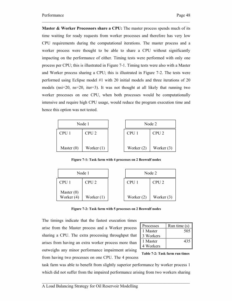
Performance Page 48 _____________________________________________________________________
_____________________________________________________________________ A Load Balancing Strategy for Oil Reservoir Modelling
Master & Worker Processors share a CPU: The master process spends much of its
time waiting for ready requests from worker processes and therefore has very low
CPU requirements during the computational iterations. The master process and a
worker process were thought to be able to share a CPU without significantly
impacting on the performance of either. Timing tests were performed with only one
process per CPU; this is illustrated in Figure 7-1. Timing tests were also with a Master
and Worker process sharing a CPU; this is illustrated in Figure 7-2. The tests were
performed using Eclipse model #1 with 20 initial models and three iterations of 20
models (nsi=20, ns=20, iter=3). It was not thought at all likely that running two
worker processes on one CPU, when both processes would be computationally
intensive and require high CPU usage, would reduce the program execution time and
hence this option was not tested.
Figure 7-1: Task farm with 4 processes on 2 Beowulf nodes
Figure 7-2: Task farm with 5 processes on 2 Beowulf nodes
The timings indicate that the fastest execution times
arise from the Master process and a Worker process
sharing a CPU. The extra processing throughput that
arises from having an extra worker process more than
outweighs any minor performance impairment arising
from having two processes on one CPU. The 4 process
task farm was able to benefit from slightly superior performance by worker process 1
which did not suffer from the impaired performance arising from two workers sharing
Processes Run time (s) 1 Master 3 Workers
505
1 Master 4 Workers
435
Table 7-2: Task farm run times
CPU 1 Master (0) Worker (4)
CPU 2
Worker (1)
CPU 1
Worker (2)
CPU 2
Worker (3)
Node 1 Node 2
CPU 1 Master (0)
CPU 2
Worker (1)
CPU 1
Worker (2)
CPU 2
Worker (3)
Node 1 Node 2

Performance Page 49 _____________________________________________________________________
_____________________________________________________________________ A Load Balancing Strategy for Oil Reservoir Modelling
a node which is discussed in the next paragraph. However, this advantage was not
enough to outperform the 5 process task farm. The timings for the two test runs are
shown Table 7-2.
Memory Bandwidth: An Eclipse model (#1) that ran for a fixed period of simulated
time and gave a near constant execution time was repeatedly executed from within a
serial version of the original NA program and the time taken for its execution was
noted. The program executed 200 initial models and one iteration of a further 200
models (nsi=200, ns=200, iter=1) giving 400 models in total. The same model was
used in the cyclically decomposing NA program and the task farm version. The model
had an almost constant execution time in serial code. The serial program used one
CPU on one node; the other CPU remained unutilised. The cyclic program used four
CPUs on two nodes; one MPI process executed on each CPU, this configuration is
illustrated in Figure 7-3. The task farm execution also used four CPUs on two nodes
using the configuration shown in Figure 7-2.
Figure 7-3: Cyclic NA processes on two Beowulf nodes
It was observed that the execution time
for an Eclipse model in serial code was
significantly shorter than for an Eclipse
model executed in parallel code. The
approximate ranges of execution times are
shown in Table 7-3; the parallel times are representative of both the cyclically
decomposing NA program and of the task farm. A relatively wider spread of model
execution times were also observed when using Eclipse model #2 with has more
variable execution times; the highest maximum recorded was higher than when run in
serial code as was the lowest minimum. The variable run times make precise
explanation of the change in execution time problematic.
Eclipse in … Run time range (s) Serial code 11.2 – 13.9 Parallel code 17.0 – 25.0
Table 7-3: Eclipse run times - Serial & Parallel
CPU 1
Cyclic Process (0)
CPU 2
Cyclic Process (1)
Node 1
CPU 1
Cyclic Process (2)
CPU 2
Cyclic Process (3)
Node 2

Performance Page 50 _____________________________________________________________________
_____________________________________________________________________ A Load Balancing Strategy for Oil Reservoir Modelling
A further test run was performed, again using the cyclic program, using three nodes
with four processes. One node was used for two processes so that both CPUs on this
node were utilised. On each of the other two nodes only one process executed so that
on each node only one CPU was in use and that other remained unutilised. This
configuration is illustrated in Figure 7-4.
Figure 7-4: Cyclic NA processes on three Beowulf nodes
When the cyclic program was run on this configuration of nodes and CPUs, the
Eclipse run times for a model on nodes 1 and 3 were in the same range as those for
runs performed using the serial code. On node 2, the Eclipse run times were still in the
approximate range 17.0 to 25.0 seconds.
The Stream benchmark [SB1] was then
used to try and identify the cause of the
poor performance when both CPUs on a
node were utilised. The Fortran Stream
benchmark program utilised [SB2]
provides information on the memory bandwidth of CPUs that are being used for a
variety of computational operations. These operations are listed in Table 7-4; the
information is taken from the Streams benchmark website [SB3].
The benchmark program creates data structures (arrays) that are too large to fit into
the lowest level of cache and tests the retrieval time of data from this lowest level of
cache when used in computational operations. The benchmark was performed on one
node utilising one CPU and then repeated on one node using both CPUs. The Intel
Pentium III processor has a level 2 cache size of 512kb [IN1] and this was verified
using the Linux-Gnu dmesg command. The array sizes of the Fortran double precision
(8 byte real) arrays were set to two million to ensure that the Level 2 cache was more
than filled.
Function Kernel Copy a(i) = b(i) Scale a(i) = q*b(i) Sum a(i) = b(i) + c(i) Triad a(i) = b(i) + q*c(i)
Table 7-4: Stream Benchmark functions [SB3]
CPU 1
Idle
CPU 2
Cyclic Process (0)
CPU 1
Cyclic Process (1)
CPU 2
Cyclic Process (2)
Node 1
CPU 1
Cyclic Process (3)
CPU 2
Idle
Node 2 Node 3

Performance Page 51 _____________________________________________________________________
_____________________________________________________________________ A Load Balancing Strategy for Oil Reservoir Modelling
The results of the Stream benchmark are shown in Table 7-5 for one node using one
CPU and in Table 7-6 for one node with both CPUs being utilised. It shows the
aggregate memory bandwidth when both CPUs on a node are utilised drops
significantly. When the memory bandwidth is considered for each CPU it indicates
that each CPU is operating with a memory bandwidth much less than half of that
available to one CPU singly employed on one node. The run times, shown as average,
minimum and maximum, all significantly increase when both CPUs on a node are
utilised. This evidence suggests that memory access time as a probable cause of the
node’s poor performance when using both CPUs on a node in memory intensive
applications.
Function Bandwidth (Mb/s) Avg Time (s) Min time (s) Max time (s) Copy 404.4745 0.0792 0.0791 0.0793Scale 408.3247 0.0789 0.0784 0.0791Add 487.0871 0.0987 0.0985 0.0990Triad 483.6028 0.0994 0.0993 0.0995
Table 7-5: Stream Benchmark (1 Node 1 CPU)
Function Bandwidth (Mb/s) Avg Time (s) Min time (s) Max time (s) Copy 380.5741 0.1684 0.1682 0.1688Scale 381.4563 0.1682 0.1678 0.1687Add 438.0321 0.2195 0.2192 0.2199Triad 438.0002 0.2196 0.2192 0.2201
Table 7-6: Stream Benchmark (1 Node 2CPUs)
A further test was conducted using a Fortran
MPI program that was written to perform
simple arithmetic with little or no memory
access. The program performed
approximately 4x10⁹ increment and
decrement operations on a double precision
variable. The run times on various CPU configurations are shown in Table 7-7. They
show that a program that has very little memory accesses runs in a consistent time
regardless of the number of CPUs being utilised. This adds some supporting evidence
that the memory bandwidth is the cause of the poor performance when both CPUs on
one node are utilised in a memory intensive application.
Processor config. Run time (s) 1 node 1 CPU 12.872 1 node 2 CPUs 12.871, 12.877 2 nodes 4 CPUs 12.870, 12.862
12.890, 12.875
Table 7-7: Non Memory Benchmark

Performance Page 52 _____________________________________________________________________
_____________________________________________________________________ A Load Balancing Strategy for Oil Reservoir Modelling
A brief search of available literature produced an article on benchmarking Intel
systems in the context of high performance clusters [PS1], albeit clusters running the
Windows operating system rather than Linux-Gnu. The article asserts that:
“Intel Pentium III processor-based systems have demonstrated a memory bottleneck in symmetric multiprocessing (SMP) systems … In memory-intensive applications processors remain idle while waiting for their memory requests to be satisfied”
While this assertion relates to Windows based platforms, it does provide supporting
evidence of memory access problems with the Intel Pentium III processor.
Master process suspension: During task farm testing on Lomond, to ensure that the
master process’s CPU usage was minimized, the master process was encouraged to
suspend itself when there were no incoming messages waiting to be processed. This
was achieved using the MPI_Iprobe subroutine call and the system subroutine sleep
(see Figure 6-8). The MPI_Iprobe subroutine checks for the presence of incoming
messages and returns a flag to indicate the presence, or otherwise, of incoming worker
messages. If there are no messages waiting to be processed then the subroutine sleep
is called and the master process suspends itself for approximately one second. The
accuracy of the sleep subroutine is platform dependent and the actual duration of
process suspension may be up to one second less than that requested [UX1]. The
argument to subroutine sleep is restricted to integer values and cannot be tuned more
finely than this. On Lomond, the use of this functionality reduced program run times.
This reduction has not been quantified owing to the unavailability of Lomond during
the second half of this project.
While this technique significantly reduces the CPU usage of the master process, it can
potentially have a negative impact on the performance of worker threads. For
example, if the master process suspends itself immediately prior to the receipt of a
worker ready request, then the worker may potentially have to wait up to
approximately one second before the message is received and a new task is allocated
to the idle processor. The negative impact would be greater when using a model with
a short run time since the wait time would be proportionately greater for a shorter
model run time.

Performance Page 53 _____________________________________________________________________
_____________________________________________________________________ A Load Balancing Strategy for Oil Reservoir Modelling
When the task farm was transferred to the Beowulf cluster, the program was timed
with and without the MPI_Iprobe/sleep functionality to quantify the benefits that it
was assumed would arise from using it. The timings from test runs indicated that the
version of the program with the sleep functionality were greater than those for the
program without it. The test runs used Eclipse model #2 with 200 initial models plus
one iteration with 200 models (nsi=200, ns=200, iter=1), a total of 400 models. The
test runs were performed with five processes (one master and four workers) running
on two nodes (four processors) using the configuration shown in Figure 7-2. In Table
7-8 the following timings are shown:
• Total time spent by Master process in subroutine tf_master
• Total time spent by Master process asleep in subroutine tf_master
• Total time spent by Worker processes waiting for a message from the Master
process
• Total program run time
Master process timings (s)
Total worker wait time after send of request for receive of message (s)
Program
Total time in tf_master
Sleep time in tf_master
Worker 1
Worker 2
Worker 3
Worker 4
Run time (s)
With Iprobe/Sleep
458.819 458.700 52.095 60.462 60.779 60.759 458.955
Without Iprobe/Sleep
401.835 N/A 0.032 0.808 1.180 0.388 401.975
Table 7-8: Task farm performance with & without Master process suspension.
The timings show that not using the MPI_Iprobe/sleep functionality resulted in
lower program run times. The time spent by the Master process in subroutine
tf_master noticeably decreased as did the time spent by worker processes waiting to
receive messages from the Master process containing a task id. It is possible that the
combination of the MPI implementation and operating system on the Beowulf cluster,
Linux-Gnu, suspends idle processes whereas on Lomond, which runs Solaris, this
does not occur. It can also be observed that Worker processes 1 and 4 which run on
the same node as the Master process have the lowest wait times. Worker 4’s wait time

Performance Page 54 _____________________________________________________________________
_____________________________________________________________________ A Load Balancing Strategy for Oil Reservoir Modelling
is slightly higher but still lower than those for processes on node 2; since Worker 4
shares a CPU with the Master process, one or the other will need to be swapped in
before the communication can complete. This is an indication that, as might be
expected, intra-node communication between CPUs is quicker than inter-node
communication between CPUs.
The sleep functionality has been left in place and can be included by use of a
compilation switch should it be needed on a different platform. Since the sleep
function input argument, which determines the duration of process suspension, is an
integer value it cannot be finely tuned. If it were possible to implement a sleep
procedure with a non integer argument then fine tuning using the finer resolution
might be possible. A sleep duration of less than one second could reduce the amount
of time spent by worker processes waiting for a task identifier thus improving the
performance of the worker process. However, if the sleep duration was reduced the
master process would spend more time active and the worker process that shares a
processor with the master process would be adversely affected and become
marginally slower. The load balancing properties of the task farm should ameliorate
the worst effects of this scenario since it is designed to give tasks to processors as they
become free and a single marginally slower worker process should not result in an
increase in processor idle time. In the absence of a sleep procedure that accepts a non
integer argument and no available platform on which to perform tests, this remains a
moot point.
Task farm communications overhead: The task farm implementation introduces
MPI communications between processes that are not present in the cyclic program.
The communication takes the form of messages from worker processes to the master
process requesting a task to perform. In return, the master process sends task identifier
to the worker process. Each model that is executed requires the sending of two MPI
messages; one by the worker process and one by the master process. If the overhead
of the communications took a significant length of time to complete, then the task
farm performance would suffer.
Timing code inserted into the NA program for worker processes calculated the total
time required for the worker processes to wait for their work request to be satisfied.

Performance Page 55 _____________________________________________________________________
_____________________________________________________________________ A Load Balancing Strategy for Oil Reservoir Modelling
The timer starts when the worker process returns from the MPI send routine used to
send the worker request and completes when the worker process returns from the MPI
receive routine that returns the task identifier for the worker process. The aggregate
worker process waiting time can then be calculated. As can be seen from Table 7-8
the time spent by worker processes waiting for a task identifier is not in any way
significant when the sleep functionality is switched off. Over two iterations the
worker wait time on each process is, at worst, approximately 0.25% of the total
program run time.
Timings were also taken on NA program runs using 320 models over ten iterations
(nsi=320, ns=320, iter=10). The time spent in subroutine tf_worker and the
aggregate time spent in subroutine forward were both calculated. The difference
between the two, which would include all MPI communications (both send and
receive) and all other non modelling computational overhead, was at worst 0.12
seconds per iteration. In most cases this was measured in hundredths of seconds rather
than tenths of seconds. Over ten iterations the total overhead should be no more than
two seconds. This would suggest that the extra MPI communication required for the
task farm functionality does not noticeably impair its performance.
Location of data files: The modelling software uses a variety of software including
Fortran code, third party packages, make files and python scripts. All these have file
i/o; each software component needs to read from and/or write to data files for each
model that is executed. Intuitively it seemed likely that using file systems on the
execution node would result in faster file access than using file systems on the
cluster’s front end. The software was modified to give the option of installing working
environments locally on the front end or remotely on the execution node. Test runs
using the same model were executed to determine the impact on execution times
when using front-end and on-node file systems. The different locations require the use
of an install script to create the necessary working directories and copy the necessary
application data files into the correct location.
Using the front-end file system required the use of temporary directories within the
working directory used for program development and execution. When using on-node
file systems on the execution node, the temporary directories were created within the

Performance Page 56 _____________________________________________________________________
_____________________________________________________________________ A Load Balancing Strategy for Oil Reservoir Modelling
/tmp file system. In both cases an installation script copied all required data files into
the working directory.
The test run used Eclipse model #2 with variable run times with additional Fortran
code with file i/o. The test runs used 200 initial models plus one iteration of 200
models (nsi=200, ns=200, iter=1) giving a total of 400 models. The cyclic and task
farm program were run on two nodes (four processors). The task farm was run with
five processes (one master and four workers). Analysis of timing information from the
test runs indicated that using on-node file systems on the execution nodes resulted in
much reduced run times both for individual models and as a consequence the overall
run time for the whole program. It was decided to use on-node file systems for
program runs while retaining the option of using front-end file systems if desired. For
example, the use of front-end file systems can be helpful using development and
testing of the task farm software. Typical values for the minimum, maximum and
average model execution times and the overall program run time are shown in Table
7-9. The times are representative of both the cyclic and task farm programs.
File system Min model
time (s) Max model time (s)
Average model time (s)
Total run time (s)
Front-end 4.5 9.5 6.3 687On-node /tmp 2.2 6.9 4.0 455
Table 7-9: Model and Program run times (Front-end and On-node).
The table shows that the minimum and maximum model execution times were greatly
reduced. The average model execution time was reduced by one third as was the
overall execution time for the whole program. This represents a significant
improvement in performance for both the cyclic and task farm programs; both
programs will benefit from the use of the /tmp on-node file system.
The effect of using on-node file systems varied across the three models and also
varied as the number of processors used was increased. In all cases the use of on-node
file systems resulted in significant reductions in the program execution time. The
cyclic program run times using on-node file systems relative to the times using front-
end file systems are shown in Figure 7-5, Figure 7-6 and Figure 7-7. The data from
which the graphs are derived is shown in Table 7-10.

Performance Page 57 _____________________________________________________________________
_____________________________________________________________________ A Load Balancing Strategy for Oil Reservoir Modelling
Eclipse Model #1: Relative Cyclic Times - Use of /tmp
0
10
20
30
40
50
60
70
80
90
100
np=4 np=8 np=16 np=24 np=32
Number of Processors
Rel
ativ
e Ti
mes
Cyclic (Front-End)=100 Cyclic (On-node)
Figure 7-5: Eclipse Model #1: Relative Cyclic Times - Use of /tmp
VIP Model: Relative Cyclic Times - Use of /tmp
0
10
20
30
40
50
60
70
80
90
100
np=4 np=8 np=16 np=24 np=32
Number of Processors
Rel
ativ
e Ti
mes
Cyclic (Front-End)=100 Cyclic (On-node)
Figure 7-6: VIP Model: Relative Cyclic Times - Use of /tmp

Performance Page 58 _____________________________________________________________________
_____________________________________________________________________ A Load Balancing Strategy for Oil Reservoir Modelling
Eclipse Model #2: Relative Cyclic Times - Use of /tmp
0
10
20
30
40
50
60
70
80
90
100
np=4 np=8 np=16 np=24 np=32
Number of Processors
Rel
ativ
e Ti
mes
Cyclic (Front-End)=100 Cyclic (On-node)
Figure 7-7: Eclipse Model #2: Relative Cyclic Times - Use of /tmp
Model np Cyclic Time
(Front End) Cyclic Time (On-Node)
ReductionTime
Reduction %
Eclipse #1 4 322m46s 297m19s 25m27s 8 8 177m01s 148m34s 28m27s 16 16 89m46s 75m21s 14m25s 16 24 66m47s 55m55s 10m52s 16 32 52m38s 41m09s 11m29s 22 VIP 4 373m57s 317m26s 56m31s 15 8 175m21s 164m28s 10m53s 6 16 92m39s 83m23s 9m16s 10 24 65m24s 57m25s 7m59s 12 32 50m44s 43m12s 7m32s 15 Eclipse #2 4 103m57s 64m21s 39m36s 38 8 73m50s 35m06s 38m44s 52 16 48m10s 17m02s 32m08s 65 24 48m13s 12m13s 36m40s 75 32 54m13s 9m00s 45m13s 83
Table 7-10: Front-End vs On-Node Run Times and Run Time Reduction
The reductions in program run times shown in Table 7-10 illustrate very clearly the
performance benefit gained from using on-node file systems. For Eclipse model #1
and the VIP model, the reduction is substantial and generally increases as the number
of processors being used increases. For Eclipse model #2 the reduction is massive.
The only difference between the NA program’s configurations used for timed runs
Performance Page 59 _____________________________________________________________________
_____________________________________________________________________ A Load Balancing Strategy for Oil Reservoir Modelling
was the location of the data files used by the modelling packages; this would seem to
be the only possible cause for the dramatic changes in the program execution times. It
would seem likely that communication between nodes and the front end of the Cluster
is either inherently slow and/or limited in speed by the number of processes that can
simultaneously use it without causing contention for resources. The two Eclipse
models show very different performance characteristics when run using front-end file
systems; Eclipse model #2 has much shorter model run times than Eclipse model #1
so it would seem likely that the effect of slower front-end file access has a
proportionately greater impact than for Eclipse model #1. The times shown in Table
7-10 for front-end program runs are the shortest times that were observed over a
number of repeated runs. There was noticeable variation across the runs for each
configuration. Examining individual model times when the front-end was used
showed than individual models often were often taking two to five times longer to
execute for Eclipse model #1 and the VIP model than when run using on-node file
systems. The performance for Eclipse model #2 was even worse with many models
sometimes running twenty times slower; that is models which would run in
approximately four seconds using on-node file systems were taking up to 80 seconds,
and sometimes longer, when using front-end file systems. The number of jobs running
on nodes that are using front-end file systems would also effect communications
between the computational nodes and the front-end. It would seem likely that the
variation in front-end times for any particular program configuration would be caused
by the number of competing processes trying to get through this communications
bottleneck. The more batch jobs that are running on nodes and trying to use front-end
file systems, the worse the performance will become. It is even possible that when
running the NA program on 32 processors that the program’s own processes by
themselves cause a bottleneck.
Elapsed time within the Models: The reservoir modelling part of the program is
performed by the module forward which can be a Fortran subroutine or written in
any other language that can be linked with the main body of the NA program. Within
this module various different software modules can be run as part of the modelling
process; this includes the third party modelling packages as well as Make files,
Python scripts and other Fortran modules. Timings for the various components

Performance Page 60 _____________________________________________________________________
_____________________________________________________________________ A Load Balancing Strategy for Oil Reservoir Modelling
highlighted that the third party software required most time to execute. The timings
for a typical single Eclipse model #1 run in serial code are shown in Table 7-11.
Eclipse model #1: Component Timings Component Software Time (s) Time (%) create_stochastic Fortran 1.80 10.42Eclipse 3rd party 15.42 89.29Makefile Make < 0.04 < 0.23calculate_misfit Fortran < 0.01 < 0.06Other Fortran Not significantTotal 17.27 100
Table 7-11: Eclipse model #1 Component Timings
It is clear that Eclipse takes the longest of all the components to execute. The Eclipse
source code is not available and hence cannot be investigated for opportunities to
optimise it. The create_stochastic Fortran subroutine uses about 10% of the
elapsed time; even if significant optimisation opportunities were to be found within
this procedure, the effect on the overall run time would be minimal.
Within the VIP model version of the forward routine there is a small amount of C++
code which invokes the VIP software. Opportunities for optimising the C++ code are
not present and would make no significant impact on the overall run time.
Eclipse model #2 uses third party software and a Python script in its version of the
forward routine; these components are contained within a small number of lines of
Fortran code. The timings for these components taken from a typical model run in
serial code are shown in Table 7-12.
Eclipse model #2: Component Timings Component Software Time (s) Time (%) Eclipse 3rd party 4.425 98.90Misfit Python 0.024 0.54Other Fortran 0.025 0.56Total 4.474 100
Table 7-12: Eclipse model #2 Component Timings
Again, it can be seen that Eclipse is the most significant component within the
modelling process. There are no opportunities for optimisation within the other
software components that will have any effect on the overall run time.

Performance Page 61 _____________________________________________________________________
_____________________________________________________________________ A Load Balancing Strategy for Oil Reservoir Modelling
Parallel Performance with Two CPUs per Node: A number of timing runs were
performed using the parallel NA programs to try and assess their performance. The
first attempt to evaluate the performance of the task farm shows the task farm run
time as a percentage of the cyclic program. More usual indicators of parallel
performance such as parallel speedup and parallel efficiency are also discussed later.
In the light of the impact of the memory bandwidth limitations it is strongly felt that
that calculated values for speedup and efficiency have some difficulties with
interpretation. Evaluating the task farm performance relative to the cyclic program
also has value since the object of the project was to improve upon the cyclic program
performance; relative performance provides a simple indication as to whether this has
been achieved. The impact on parallel model execution times when both CPUs on a
node are utilised could make the calculation of any performance indicators based on
the serial execution time potentially misleading. On a platform without the memory
bandwidth problem, the parallel speedup and parallel efficiency values might be
significantly better. For all three models the following problem size has been used:
nsi=320, ns=320, nr=160, iter=10. In all graphs the cyclic run time has been
normalised to 100. The raw data is shown in §12.
The relative run times for Eclipse model #1 are shown in Figure 7-8. The task farm
performance would seem to bring very little benefit except in when run on 24
processors. A factor in the superior task farm performance may be due in some part to
the number of models (ns=320) not being exactly divisible by the number of
processors (np=24); eight processes will have one extra task to perform on each
iteration. Later discussion will show that the memory bandwidth problems are also
likely to have had a major impact on the performance of the parallel programs.

Performance Page 62 _____________________________________________________________________
_____________________________________________________________________ A Load Balancing Strategy for Oil Reservoir Modelling
Eclipse Model #1 (Fixed Time) Relative Times
0102030405060708090
100110
P=4 np=8 np=16 np=24 np=32
Number of Processors
Rel
ativ
e Ti
mes
Cyclic=100 Task Farm (Unsorted) Task Farm (Sorted)
Figure 7-8: Eclipse Model #1: Relative Times
For the VIP model, the performance of the task farm was variable when compared to
the cyclic program. The task farm performance beats the cyclic program in most cases
but not for np=4. As with Eclipse model #1, environmental problems are also believed
to have had some impact on parallel program performance. The relative run times for
the VIP model are shown in Figure 7-9.
Vip Model (Fixed Time) Relative Times
0102030405060708090
100110
np=4 np=8 np=16 np=24 np=32
Number of Processors
Rel
ativ
e Ti
mes
Cyclic=100 Task Farm (Unsorted) Task Farm (Sorted)
Figure 7-9: VIP Model: Relative Times
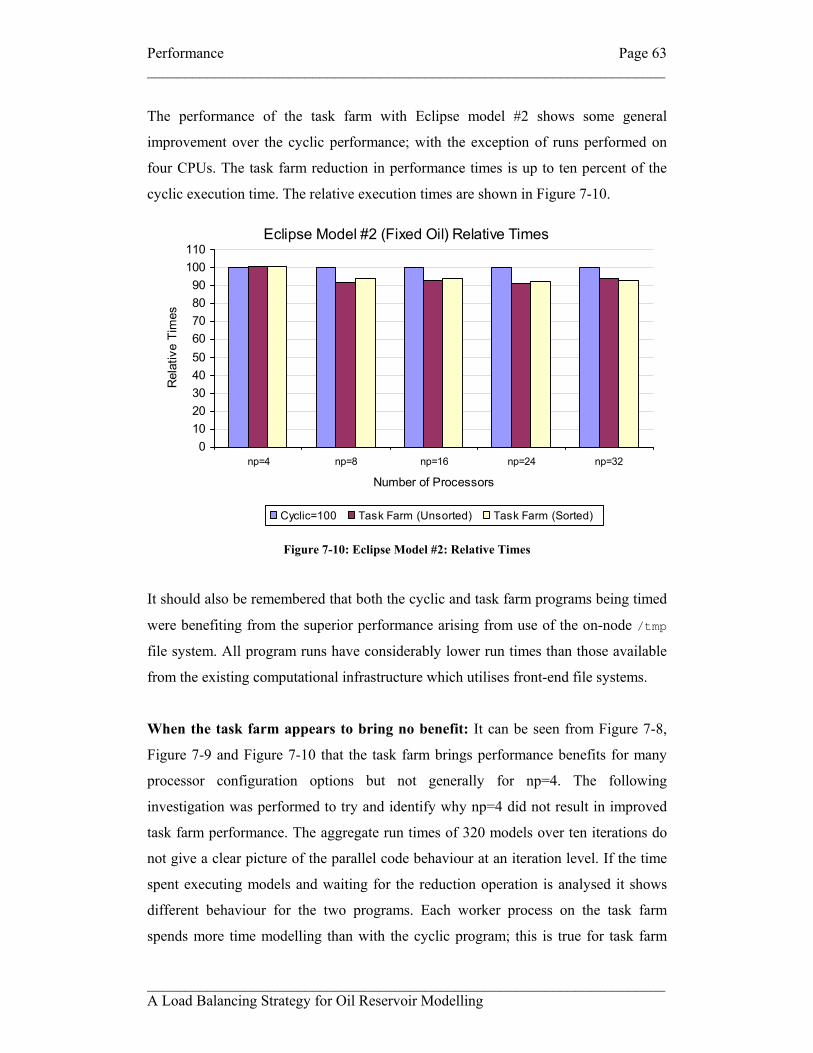
Performance Page 63 _____________________________________________________________________
_____________________________________________________________________ A Load Balancing Strategy for Oil Reservoir Modelling
The performance of the task farm with Eclipse model #2 shows some general
improvement over the cyclic performance; with the exception of runs performed on
four CPUs. The task farm reduction in performance times is up to ten percent of the
cyclic execution time. The relative execution times are shown in Figure 7-10.
Eclipse Model #2 (Fixed Oil) Relative Times
0102030405060708090
100110
np=4 np=8 np=16 np=24 np=32
Number of Processors
Rel
ativ
e Ti
mes
Cyclic=100 Task Farm (Unsorted) Task Farm (Sorted)
Figure 7-10: Eclipse Model #2: Relative Times
It should also be remembered that both the cyclic and task farm programs being timed
were benefiting from the superior performance arising from use of the on-node /tmp
file system. All program runs have considerably lower run times than those available
from the existing computational infrastructure which utilises front-end file systems.
When the task farm appears to bring no benefit: It can be seen from Figure 7-8,
Figure 7-9 and Figure 7-10 that the task farm brings performance benefits for many
processor configuration options but not generally for np=4. The following
investigation was performed to try and identify why np=4 did not result in improved
task farm performance. The aggregate run times of 320 models over ten iterations do
not give a clear picture of the parallel code behaviour at an iteration level. If the time
spent executing models and waiting for the reduction operation is analysed it shows
different behaviour for the two programs. Each worker process on the task farm
spends more time modelling than with the cyclic program; this is true for task farm

Performance Page 64 _____________________________________________________________________
_____________________________________________________________________ A Load Balancing Strategy for Oil Reservoir Modelling
processes that execute fewer models than a cyclic process. The aggregate modelling
time for the task farm is also greater than for the cyclic program. The task farm
worker processes also spend significantly less time waiting for the reduction
operation; this is true on individual basis and also aggregately. These observations
seem to be specific to running with np=4.
Table 7-13, Table 7-14 and Table 7-15 show the aggregate times spent by each
program process performing modelling and waiting for the reduction and also the
number of models executed by each process. The bookkeeping times are not at all
significant, usually much less than one second per iteration, and have not been
included; this tallies with information from the program author that bookkeeping time
might typically be a few tenths of one per-cent of the total run time [MS1]. The
details are shown for cyclic processes 0 to 3 and for task farm worker processes 1 to 4
(without task sorting). The data is taken from the model run with ten iterations of 320
models run on four processors.
Eclipse Model #1: Aggregate Program Data Cyclic Modelling
Time (s) Reduction Time (s)
Num Models
TF Worker
Modelling Time (s)
Reduction Time (s)
Num Models
0 17,446 387 880 1 17,857 25 8671 17,098 735 880 2 17,807 78 8932 17,798 35 880 3 17,812 73 8943 17,802 31 880 4 17,828 53 866Total 70,144 1,188 3520 Total 71,304 229 3520
Table 7-13: Eclipse Model #1: Aggregate Iteration Times
VIP Model: Aggregate Program Data Cyclic Modelling
Time (s) Reduction Time (s)
Num Models
TF Worker
Modelling Time (s)
Reduction Time (s)
Num Models
0 18,958 83 880 1 18,958 94 8881 18,929 111 880 2 18,970 85 8712 18,729 311 880 3 18,970 85 8713 18,679 361 880 4 18,984 68 890Total 75,295 866 3520 Total 75,882 352 3520
Table 7-14: VIP Model: Aggregate Iteration Times

Performance Page 65 _____________________________________________________________________
_____________________________________________________________________ A Load Balancing Strategy for Oil Reservoir Modelling
Eclipse Model #2: Aggregate Program Data
Cyclic Modelling Time (s)
Reduction Time (s)
Num Models
TF Worker
Modelling Time (s)
Reduction Time (s)
Num Models
0 3,806 51 880 1 3,862 13 8701 3,715 142 880 2 3,865 11 8892 3,811 46 880 3 3,859 18 8853 3,802 55 880 4 3,860 15 876Total 15,134 294 3520 Total 15,346 57 3520
Table 7-15: Eclipse Model #2: Aggregate Iteration Times
For each of the three models it can be seen that the task farm takes longer than the
cyclic program to perform the same modelling tasks. For Eclipse model #1, the task
farm takes nearly 20 minutes longer than the cyclic program for ten iterations. It is not
unusual for the NA program to be run over several hundred iterations which would
make the cumulative effect much greater. It is not likely that the inter-processor MPI
communications would cause the task farm modelling execution time to increase so
significantly since, as has already been discussed, they add very little to the execution
time. The aggregate time waiting for the reduction is lower for the task farm. In most
cases the individual task farm waiting times are lower than for the cyclic program,
however, not enough to offset the additional modelling time.
Further information can be found by looking at the modelling times and reduction
waiting times for individual iterations. Unfortunately, the disparity between modelling
and reduction times means that a graphical representation provides little clarity. Table
7-16 shows details of the first four iterations from the NA program run for Eclipse
model #1. The details are shown for cyclic processes 0 to 3 and for task farm worker
processes 1 to 4. The following data items are displayed:
• Mod(n) Modelling time for iteration n.
• Red(n) Reduction waiting time for iteration n.
• Iter(n) Total time for iteration n i.e. Mod(n) + Red(n)
• Models(n) Number of models executed in iteration n.
The small differences between total iteration times, Iter(n), within each program
iteration arise from the small bookkeeping time and from rounding errors.

Performance Page 66 _____________________________________________________________________
_____________________________________________________________________ A Load Balancing Strategy for Oil Reservoir Modelling
Cyclic
(0) Cyclic (1)
Cyclic (2)
Cyclic (3)
Worker (1)
Worker (2)
Worker (3)
Worker (4)
Mod(0) s 1594.40 1570.26 1600.59 1604.49 1623.90 1628.20 1619.44 1615.34Red(0) s 10.08 34.23 3.90 0 4.34 0 8.77 12.88Iter(0) s 1604.48 1604.49 1604.49 1604.49 1628.24 1628.20 1628.21 1628.22Models(0) 80 80 80 80 79 82 81 78Mod(1) s 1598.17 1561.71 1582.45 1591.79 1616.15 1614.12 1612.63 1608.32Red(1) s 0 36.46 15.71 6.38 0.04 2.05 3.55 7.79Iter(1) s 1598.17 1598.17 1598.16 1598.17 1616.19 1616.17 1616.18 1616.11Models(1) 80 80 80 80 80 80 80 80Mod(2) s 1593.54 1566.54 1606.02 1593.95 1625.01 1622.47 1619.05 1624.35Red(2) s 12.48 39.48 0 12.07 0.03 2.73 6.15 0.74Iter(2) s 1606.02 1606.02 1606.02 1606.02 1625.04 1625.20 1625.20 1625.09Models(2) 80 80 80 80 78 82 82 78Mod(3) 1591.08 1559.96 1632.69 1636.36 1616.58 1599.70 1602.36 1612.78Red(3) 45.29 76.40 3.68 0 0.04 16.96 14.31 3.75Iter(3) s 1636.37 1636.36 1636.37 1636.36 1616.62 1616.66 1616.67 1616.53Models(3) 80 80 80 80 80 80 80 80
Table 7-16: Eclipse Model #1: Individual Iteration Details
In most cases the cyclic modelling time is less than the task farm time and the cyclic
reduction time is greater than for the task farm. In general it would seem that the task
farm takes longer to perform the same the same modelling activities as the cyclic
program but waits for less reduction time than the cyclic program. The task farm
loading of CPUs is more evenly balanced but slower. It is worth emphasising that this
means that task farm has improved the load balancing capabilities of the NA program;
the computational load is being more evenly spread across the available processors. It
is suggested that, if using the cyclic program, when one CPU finishes its tasks the
other CPU has exclusive usage of the shared node memory and that the memory
bandwidth problem does not occur while the busy CPU completes its remaining tasks.
In contrast, the task farm will have both CPUs in use for almost all its model
execution time and the memory bandwidth problem will always be present. The cyclic
program will execute a small number of models much more quickly when only one
CPU is in use than the task farm which will always have the slower model execution
time. Intuitively, it seems likely that running with np=4 will result in the largest cyclic
program imbalance and hence the longest period when parallel models will execute in
“serial time”. It is slightly difficult, but probably possible, to prove this by cross
checking individual model times across processes.
Performance Page 67 _____________________________________________________________________
_____________________________________________________________________ A Load Balancing Strategy for Oil Reservoir Modelling
When the task farm reduces execution times: The graphs of task farm execution
time relative to the cyclic program also show that execution times are reduced for
np>4. For Eclipse model #1 and the VIP model, the reduction is small. It is more
noticeable for Eclipse model #2; to illustrate how the task farm approach has worked,
the execution times for the first four iterations from both parallel programs, for np=8,
were analysed in detail. The data is shown in Table 7-17 in the same format used for
Table 7-16. As before, examining the modelling and reduction times for each iteration
shows how the overall execution time is composed.
The aggregate modelling time within each iteration is similar for both programs; the
minimum difference is two seconds (for iteration 0) and the maximum about 28
seconds (for iteration 2). The task farm aggregate total is sometimes less than the
cyclic program, sometimes more. Modelling times for individual processors within an
iteration vary for both programs but are far more widely spread for the cyclic
program. The task farm times are in a much narrower range; the work performed by
each processor is far more equal than for the cyclic program. The number of models
executed by the cyclic program on each processor is fixed for each iteration; the task
farm processors execute a variable number of models. Some task farm processors
execute more models and some fewer. This is the load balancing that the task farm set
out to achieve.
As a result of the task farm processors completing their work within a smaller window
of time than the cyclic program, each processor has to spend less time waiting for the
reduction operation to take place. The maximum task farm waiting time for the four
iterations shown is 4.18 seconds whereas for the cyclic program the maximum is
34.45 seconds (both times from iteration 0). The task farm reduction waiting times are
measured in seconds, the cyclic reduction waiting times are measured in tens of
seconds.
The effect of the reduced waiting is to make the task farm faster over each iteration.
The task farm iteration times are up to 18 seconds shorter than the cyclic iteration
times. The task farm time saving accumulates over each iteration; this gives a reduced
program execution time.
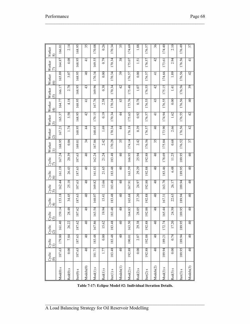
Performance Page 68 _____________________________________________________________________
_____________________________________________________________________ A Load Balancing Strategy for Oil Reservoir Modelling
Wor
ker
(8) 16
6.81
2.14
168.
95
35
170.
08
0.26
170.
34
35
174.
69
1.88
176.
57
36
174.
40
2.10
176.
49
37
Wor
ker
(7) 16
4.87
4.08
168.
95
41
169.
55
0.79
170.
34
38
175.
07
1.51
176.
57
42
173.
61
2.94
176.
56
41
Wor
ker
(6) 16
5.89
3.07
168.
95
40
170.
34
0.00
170.
34
39
176.
57
0.00
176.
57
41
174.
66
1.89
176.
56
42
Wor
ker
(5) 16
6.17
2.78
168.
95
43
169.
96
0.38
170.
34
42
175.
48
1.07
176.
55
42
175.
15
1.41
176.
56
39
Wor
ker
(4) 16
4.77
4.18
168.
95
41
167.
76
2.58
170.
34
43
175.
76
0.78
176.
55
43
176.
55
0.00
176.
56
40
Wor
ker
(3) 16
5.37
3.58
168.
95
42
170.
15
0.19
170.
34
44
175.
65
0.92
176.
57
41
174.
94
1.62
176.
55
42
Wor
ker
(2) 16
7.21
1.74
168.
95
44
168.
65
1.69
170.
34
44
176.
18
0.39
176.
57
40
173.
90
2.66
176.
56
42
Wor
ker
(1) 16
8.95
0.06
169.
01
34
167.
86
2.42
170.
28
35
174.
14
2.42
176.
56
35
175.
84
0.68
176.
52
37
Cyc
lic
(7) 16
7.24
20.3
9
187.
63
40
162.
24
21.2
4
183.
48
40
166.
95
25.9
4
192.
88
40
178.
69
11.2
5
189.
95
40
Cyc
lic
(6) 16
1.19
26.4
3
187.
63
40
161.
83
21.6
5
183.
48
40
163.
59
29.2
9
192.
88
40
183.
46
6.48
189.
95
40
Cyc
lic
(5) 16
2.44
25.1
8
187.
63
40
169.
82
13.6
6
183.
48
40
167.
91
24.9
7
192.
88
40
163.
78
26.1
7
189.
94
40
Cyc
lic
(4) 15
3.18
34.4
5
187.
63
40
168.
07
15.4
1
183.
48
40
165.
68
27.2
0
192.
88
40
167.
31
22.6
3
189.
94
40
Cyc
lic
(3) 15
9.14
28.4
8
187.
62
40
163.
54
19.9
4
183.
48
40
164.
83
28.0
5
192.
88
40
165.
44
24.5
0
189.
95
40
Cyc
lic
(2) 16
1.40
26.2
2
187.
62
40
167.
86
15.6
2
183.
48
40
163.
50
29.3
8
192.
88
40
172.
74
17.2
0
189.
95
40
Cyc
lic
(1) 17
9.80
7.84
187.
63
40
183.
48
0.00
183.
48
40
190.
01
2.87
192.
88
40
189.
21
0.74
189.
94
40
Cyc
lic
(0) 18
7.63
0.00
187.
63
40
181.
71
1.77
183.
48
40
192.
88
0.00
192.
88
40
189.
94
0.00
189.
95
40
Mod
(0) s
Red
(0) s
Iter(
0) s
Mod
els(
0)
Mod
(1) s
Red
(1) s
Iter(
1) s
Mod
els(
1)
Mod
(2) s
Red
(2) s
Iter(
2) s
Mod
els(
2)
Mod
(3) s
Red
(3) s
Iter(
3) s
Mod
els(
3)
Table 7-17: Eclipse Model #2: Individual Iteration Details.

Performance Page 69 _____________________________________________________________________
_____________________________________________________________________ A Load Balancing Strategy for Oil Reservoir Modelling
Distribution of model execution times: As has been discussed Eclipse model #1 ran
more slowly in parallel code than it did on serial code. The cause of this has been
suggested as being the memory bandwidth problem. The individual model times for
the VIP model and Eclipse model #2 also had differing characteristics in serial code
and parallel code. The effect is very noticeable in Eclipse model #1 but less so for the
other models where the impact of the effect, if indeed memory is the problem, is more
ambiguous. The results from a number of test runs were analysed in more detail and
the individual model times banded accorded to their execution times. In all cases 320
models and ten iterations were used (nsi=320, ns=320, iter=10) giving a total of 3520
models run on four processors. Task sorting was not used for the task farm runs. The
serial times use front-end file access; they would probably be quicker for on-node file
access. The raw data can be found in §12.
Beginning with the simple case of Eclipse model #1, it can be easily demonstrated
that nearly all parallel model times were significantly higher than when run in serial
code. The distribution of run times is shown in Figure 7-11.
Eclipse Model #1: Serial & Parallel Run Time Distribution
0
500
1000
1500
2000
13.x 14.x 15.x 16.x 17.x 18.x 19.x 20.x 21.x 22.x 23.x
Execution Time (seconds)
Num
ber o
f Mod
els
Serial Cyclic (np=4) Task Farm (np=4)
Figure 7-11: Eclipse Model #1: Serial & Parallel Run Time Distribution

Performance Page 70 _____________________________________________________________________
_____________________________________________________________________ A Load Balancing Strategy for Oil Reservoir Modelling
It is immediately apparent from the graph that both cyclic and task farm model
execution times are longer than for the serial program. In this program run the cyclic
program ran 27 models in less than 18 seconds and the task farm only nine. It is
suggested that the few parallel models that run in “serial time” are models at the end
of each iteration when one process on a node has finished and the other process on the
node has exclusive access to memory. The cyclic load imbalance causes one process
per node to have longer periods of exclusive access to memory while the other
process is waiting for the synchronising reduction. The load imbalance in this case
aids the cyclic program by letting it run some models more quickly. The task farm
spends less time waiting for the synchronizing reduction because of its better load
balancing. The window in which one task farm process on a node will have exclusive
use of memory is therefore much smaller and hence the number of task farm models
run in “serial time” is smaller.
Interpreting the distribution of run times for the VIP model is more difficult. Using
one second bands to group model run times showed that majority of serial and parallel
run times were in the range of 17 to 24 seconds. For the serial times, 60% were
around 21 seconds whereas the parallel times were more widely spread. In the central
region of the graph, the time bands were reduced to one quarter of a second and this
graph is shown in Figure 7-12.
VIP Model: Serial & Parallel Run Time Distribution
0
500
1000
17.x-20.00
20.00-20.25
20.25-20.50
20.50-20.75
20.75-21.00
21.00-21.25
21.25-21.50
21.50-21.75
21.75-22.00
22.00-22.25
22.25-22.50
22.50-22.75
22.75-23.00
23.x 24.x-28.9
Execution Time (seconds)
Num
ber o
f Mod
els
Serial Cyclic (np=4) Task Farm (np=4)
Figure 7-12: VIP Model: Serial & Parallel Run Time Distribution

Performance Page 71 _____________________________________________________________________
_____________________________________________________________________ A Load Balancing Strategy for Oil Reservoir Modelling
The graph shows some a clear central grouping of serial run times in the range 21
seconds to 22 seconds. The parallel run times are more widely distributed and show
two peaks in the distribution. One peak is below the serial central peak, at about 20.75
to 21.00 seconds, indicating models that run more quickly in parallel code than in
serial code. The second peak is above the serial central peak, at about 21.75 to 22.00
seconds, indicating models that run more slowly in parallel code. The distribution
parallel model times also has a noticeable dip in the central region where serial run
times are most tightly grouped. It is difficult to assess what, if any, the overall effect
of the distribution of the parallel model execution times is likely to be. The cause of
the differing distribution characteristics cannot be readily identified.
The Eclipse model #2 run times were also broken down into smaller time bands as has
been done for the VIP model; the higher level graph provided little insight. The serial
run times have a distinct central peak. The task farm run times had a wider range both
above and below the serial run times. The peak value of the cyclic run times indicated
lower run times for the cyclic program than for the serial code. The Eclipse model #2
run time distribution is shown in Figure 7-13.
Eclipse Model #2: Serial & Parallel Run Time Distribution
0
500
1000
2.00-3.00
3.00-3.25
3.25-3.50
3.50-3.75
3.75-4.00
4.00-4.25
4.25-4.50
4.50-4.75
4.75-5.00
5.00-5.25
5.25-5.50
5.50-5.75
5.75-6.00
6.00-7.50
Execution Time (seconds)
Num
ber o
f Mod
els
Serial Cyclic (np=4) Task Farm (np=4)
Figure 7-13: Eclipse Model #2: Serial & Parallel Run Time Distribution

Performance Page 72 _____________________________________________________________________
_____________________________________________________________________ A Load Balancing Strategy for Oil Reservoir Modelling
The serial times are once again centrally grouped mostly in a range of 4.00 to 5.25
seconds. The task farm run times, again, show two peaks indicating a group of times
both below and above the serial times. The cyclic times show a distinct peak at lower
ranges than the serial run times indicating that many cyclic program model run times
are shorter than for the serial program. As with the VIP model, interpreting the effect
of the run time distributions on the overall program execution time is difficult and
attributing a cause to the differences in distributions cannot be easily done.
Parallel Speedup and Parallel Efficiency: Having timed serial and parallel program
executions it is possible to calculate values for parallel speedup and parallel
efficiency. These will give an indication of how the NA application is performing on
the Beowulf Cluster and how effectively it is making use of the additional processors
available with each parallel run. The results must be considered in the context of the
memory bandwidth problem which has been shown to place the program at a
handicap when executing Eclipse model #1 in parallel code. It should also be
remembered that there may be underlying environmental factors that affect the serial
and parallel run times; this may result in speedup and efficiency values that are not
based on comparing like for like. Parallel speedup graphs for the cyclic program and
task farm program with unsorted tasks are shown in Figure 7-14 and Figure 7-15.
The serial run times do not have the benefit of using the /tmp file system; if they had
then the speedup and efficiency values would probably be a little lower. The values in
the graphs show the speedup and efficiency of the new computational infrastructure
(on-node) relative to the existing serial computational infrastructure (front-end) The
raw data can be found in §12. The speedup values for the cyclic program and the task
farm program indicate that both parallel programs are performing quite well. For the
VIP model and Eclipse model #2 the speedup is very similar for both parallel
programs; in Figure 7-14 the two plot lines are almost identical. The speedup for
Eclipse model #1 also indicates that the parallel performance is good despite the
problems that the model has with memory bandwidth problems.

Performance Page 73 _____________________________________________________________________
_____________________________________________________________________ A Load Balancing Strategy for Oil Reservoir Modelling
Cyclic NA: Parallel Speedup
0
10
20
30
0 5 10 15 20 25 30 35Number of processors
Spe
edup
EC #1 VIP EC #2 Ideal
Figure 7-14: Cyclic NA: Parallel Speedup
Task Farm NA: Parallel Speedup
0
10
20
30
0 5 10 15 20 25 30 35Number of processors
Spee
dup
EC #1 VIP EC #2 Ideal
Figure 7-15: Task Farm NA: Parallel Speedup
It should also be remembered that the VIP model and Eclipse model #2 may be
hindered by hardware performance problems that might be impairing their
performance. Despite the possible existence of these problems the speedup is close to
being linear for the task farm when running the VIP model and Eclipse model #2. For
Eclipse model #2 the speedup is better than ideal for 4, 8, 16 and 24 processors. The
speedup for Eclipse model #1 is not linear but is still good. The cyclic program

Performance Page 74 _____________________________________________________________________
_____________________________________________________________________ A Load Balancing Strategy for Oil Reservoir Modelling
speedup is lower than for the task farm; for Eclipse model #1 the difference is very
small.
Parallel efficiency values were also calculated for both the cyclic and task farm
programs. Efficiency values indicate how effectively an application makes use of
additional processors when the application is run across an increasing number of
processors. Parallel efficiency graphs for the cyclic program and task farm program
with unsorted tasks are shown in Figure 7-16 and Figure 7-17. The raw data can be
found in §12.
Cyclic NA: Parallel Efficiency
0.0
0.2
0.4
0.6
0.8
1.0
1.2
0 5 10 15 20 25 30 35Number of processors
Effic
ienc
y
EC #1 VIP EC #2
Figure 7-16: Cyclic NA: Parallel Efficiency
Task Farm NA: Parallel Efficiency
0.0
0.2
0.4
0.6
0.8
1.0
1.2
0 5 10 15 20 25 30 35Number of processors
Effi
cien
cy
EC #1 VIP EC #2
Figure 7-17: Task Farm NA: Parallel Efficiency

Performance Page 75 _____________________________________________________________________
_____________________________________________________________________ A Load Balancing Strategy for Oil Reservoir Modelling
The efficiency graphs show that the parallel NA programs can make effective use of
additional processors. For both of the parallel programs the Eclipse model #1 makes
less effective use of additional processors; both programs have efficiency values for
this model in the range 0.80 to 0.90. Although this is less than for the other two
models, the efficiency values are still quite good. For the VIP model and Eclipse
model #2, the efficiency values are in the range 0.93 to 1.07. The task farm makes
particularly effective use of additional processors for Eclipse model #2; the efficiency
values are in the range 0.99 to 1.07. Efficiency values greater than 1 indicates better
than ideal usage of additional processors. This suggests that the aggregate effect of the
distribution of parallel model times might be beneficial to the overall program
execution time and hence the parallel efficiency. The Eclipse model #1 efficiency
values are lower than for the other two models; this indicates that additional
processors are not being so effectively utilised. This would seem reasonable given
what has been discovered concerning the performance of CPUs when Eclipse model
#1 is executed in parallel code.
In all program runs performed, the parallel efficiency values are greater than 0.7 or
70% which was the efficiency figure supplied by the project sponsor. For Eclipse
model #1 the parallel efficiency of over 80% falls short of the 95% target efficiency
goal. For the VIP model and Eclipse model #2 the efficiency values are in many cases
over 0.95 or 95% indicating that the target efficiency goal has been achieved in many
cases.
Fewer models, more iterations: A limited number of timed test runs were performed
using fewer models and more iterations. The NA program settings were nsi=ns=32,
nr=16, np=4 and iter=200. Using lower values of ns is in more in keeping with the
project sponsor’s current usage of the NA program. The run times of the cyclic
program and the task farm (without task sorting) are shown in Table 7-18.
Cyclic Task farm Reduction Reduction % EC1 608m11s 583m41s 24m30s 4.03 VIP 655m12s 653m33s 1m39s 0.25 EC2 133m53s 123m38s 10m15s 7.66
Table 7-18: Cyclic & Task Farm Timings (ns=32, iter=200)

Performance Page 76 _____________________________________________________________________
_____________________________________________________________________ A Load Balancing Strategy for Oil Reservoir Modelling
Once again, Eclipse model #2 shows the best task farm performance improvement.
The reduction in execution time for Eclipse model #1 is smaller and for the VIP
model, the difference is negligible. In order to try and further understand the
conditions under which the task farm might be
effective, the run time variability was briefly
examined. Table 7-19 shows typical values of the
mean model run time within an iteration for each
model and also the standard deviation of the model
times within the same iteration. The standard deviation gives a measure of the spread
of run times. The spread of values for Eclipse model #1 and the VIP model relative to
the mean run time is much smaller than for Eclipse model #2. This is perhaps an
indication that Eclipse model #1 and the VIP model run times do not vary sufficiently
for the task farm to bring load balancing benefits. The spread of run times for Eclipse
model #2 is much greater when the mean run time is considered. It is possible that a
statistical analysis of serial run times could highlight models that would benefit from
task farm usage. The behaviour of the task farm when using different values of ns
remains to be fully explored.
7.5 Task Sorting Effectiveness
The task farm program was timed for all three models with and without task sorting.
The method of sorting was to assume that the execution time for a model would be
approximately determined by the execution time of its parent model (see §5.2). The
effectiveness of the chosen heuristic in ordering tasks by descending execution times
was to be to evaluated by means of Spearman’s rho (§7.3).
The effect on the task farm performance for all models in the test runs performed is at
best neutral and at worst negative. As can be seen from Figure 7-8, Figure 7-9 and
Figure 7-10, the task farm with task sorting often performed worse than when task
sorting was not present.
The values of Spearman’s rho indicate whether there is any correlation between the
actual run time rankings and the predicted run time rankings. All values of
Spearman’s rho for the runs executed lay within the range -0.15 to +0.15; the majority
Mean (s) StDEC1 22.5 0.7VIP 23.1 2.2EC2 4.5 1.1
Table 7-19: Mean & Standard Deviation

Performance Page 77 _____________________________________________________________________
_____________________________________________________________________ A Load Balancing Strategy for Oil Reservoir Modelling
of the values were within the much smaller range -0.05 to +0.05. Using the chosen
interpretation of Spearman’s rho (Table 7-1), or for that matter any other
interpretation available from statistic literature, there is at best very weak correlation
between predicted and actual run time orderings and then only in a very few cases. In
general the values of Spearman’s rho indicate no correlation between the actual and
predicted execution time rankings.
There are a number of reasons why this may be occurring; it is not necessarily the
case that the chosen sorting heuristic is as invalid as the correlation values would
suggest. The reasons are listed below and discussed in detail:
• The effects of the memory bandwidth problem.
• The small number of iterations used.
• Invalid sorting heuristic.
• Properties of the models used.
• Effect of the search parameters ns and nr.
• Invalid method of evaluation.
Memory bandwidth: The memory bandwidth problem has been shown to cause
significant variations in model execution time. The sorting heuristic relied on the
properties of the model itself. It was believed that parameter values that were close
together in the parameter space might result in models that had similar execution
times. The effect of the memory bandwidth problem means that the model execution
time is no longer only dependent on the model parameters but also on hardware
influences such as memory access times. The chosen heuristic did not, and given the
nature of the memory bandwidth problem could not, include factors arising from
hardware underperformance. It may well be the case that on a platform without the
hardware problems experienced on the Beowulf cluster that the chosen heuristic
might have a beneficial effect.
Number of iterations: The test runs of the task farm program have used a small
number of iterations; it is not uncommon for several hundred iterations to be
performed when using the modelling software. As the number of iterations increases,

Performance Page 78 _____________________________________________________________________
_____________________________________________________________________ A Load Balancing Strategy for Oil Reservoir Modelling
the region or regions of parameter space being sampled become smaller and more
localised as shown by the darker areas of Figure 2-1(d). It may the case that after only
ten iterations the parameter values are not sufficiently localised for models to have
similar properties and execution times to those of the parent model. Longer runs of
say hundreds of iterations might show better correlation as the parameter values used
for models are selected from smaller and smaller regions of parameter space.
Invalid sorting heuristic: It is quite possible that the chosen heuristic is simple not
valid or not sophisticated enough. The chosen heuristic was selected for simplicity of
understanding and ease of implementation (§5.2). The development of an apposite
sorting process might require detailed knowledge of the model and modelling
package; this would require petroleum science expertise rather than computational
science expertise and as such falls outside the scope of this project. Further
investigation in this area might well prove fruitful.
Model properties: It may be the case that the chosen heuristic is not suitable for the
models that have been used. It is quite possible that for the models used there is no
correlation between a model’s run time and the run time of the parent model. The
chosen heuristic may be more successful with other models from the project sponsor’s
model base.
Search Parameters: As has been previously discussed (§7.3) a number of intuitive
hypotheses were proposed as to how effective the task sorting algorithm might be for
different types of search of the parameter space. It may be the case that using different
values of ns and nr to perform more exploratory or more exploitative searches might
result in the task sorting algorithm being more effective. The number of NA program
runs that has been performed has been limited and has only used a small set of values
for ns and nr. Further investigations might yield more information.
Evaluation Method: The implemented usage of Spearman’s rho may not be an
appropriate method of evaluation. Some form of correlation has been searched for in
the individual model times. It may be the case that more sophistication is required and
that correlation between the ordering of each group of ns/nr models (§5.2) within each
iteration should be sought.

Conclusions Page 79 _____________________________________________________________________
_____________________________________________________________________ A Load Balancing Strategy for Oil Reservoir Modelling
8. Conclusions
The path taken by the project diverged significantly from the original planned
schedule of work. This was unavoidable owing to the unforeseeable and unexpected
discoveries made when investigating the performance of the parallel NA programs
running on the Heriot-Watt Beowulf cluster. The combination of application software
and platform hardware had originally seemed to be reasonably mature and well
understood; this proved not to be the case. Investigating the discoveries regarding the
memory bandwidth problem and the benefits of using of on-node file systems made
completion of some tasks impractical owing to the additional work that was
undertaken and the project time constraints. For example measuring the NA task farm
performance in terms of parallel speedup and parallel efficiency could have been
more widely explored over a larger range of values of ns, nr and np. The differing
performance characteristics of modelling software in serial and parallel code have
produced performance results that need to be interpreted carefully and not necessarily
accepted entirely at face value.
Some of the original planned tasks and some of the planned analyses have not been
completed; some cannot be really considered to have started. Progress has been made
in a number of areas. The knowledge gained in the course of this project has given
interesting insights into what were previously poorly understood or unknown aspects
of the platform and application combination. The project has delivered good results in
the following areas:
• The delivery of correctly functioning software
• An extension to the functionality of the computational infrastructure
• Increased understanding of the Beowulf Cluster’s performance and behaviour.
Correctly functioning software: The design imperatives (§6.1) that were defined
before the start of the task farm implementation were successfully adhered to. Some
examples of successful compliance with the design imperatives follow. The code has
been simplified (imperative 1) and no refactoring in of removed code (Fortran 77
compatibility and the original program author’s toolkit) is required [MC1]. The new

Conclusions Page 80 _____________________________________________________________________
_____________________________________________________________________ A Load Balancing Strategy for Oil Reservoir Modelling
task farm source code is encapsulated within new subroutines (imperative 2) with
names beginning “tf_”. No cosmetic changes for the purpose of beautifying the
existing source code were made (imperative 3). The small number of modifications to
existing subroutines were made in the local style (imperative 4) and clearly
highlighted to warn future developers of their presence. All changes to existing code
lines have been enclosed within “! TF” comment delimiters. New subroutines were
implemented in this programmers preferred style (imperative 5) which is believed to
be sufficiently clear not to give future developers too many difficulties of
comprehension.
Verification of the output produced by the task farm was a high priority
implementation goal (§6.2.1) and the steps taken to ensure the validity of the results
have already been described (§6.4). Incorrect results, however quickly produced,
would not have brought any benefit to the NA user community. The task farm NA
program produces results that are the same as those produced by the serial NA
program and by the cyclically decomposing NA program. The only exceptions are
well understood and explainable. The exceptions arise from occasional failures of
models due to data file corruption and the sequencing of model execution. The task
farm itself functions as proposed by allocating tasks to processors when they become
available and the desired computational performance improvements have been
realised in some of the timed program runs. Improved load balancing by the task farm
manifests itself through lower reduction waiting times. The task sorting software
functions as intended although, again, it did not result in any performance
improvement. It provides a starting point for further investigations in this area and the
sorting related software can be easily modified to accommodate other sorting
algorithms. As well as producing correct results the task farm software has shown
itself to be reliable, robust and, thus far, error free over the course of the test runs that
have been conducted; its reliability is high.
Computational infrastructure: The task farm functionality can be easily added to
the existing NA program environment. The task farm provides an alternative method
of execution for modelling problems that can be selected at execution time by means
of a run time parameter. Any run of the NA program can use either the cyclic
decomposition or the task farm option. New or existing models can be timed to

Conclusions Page 81 _____________________________________________________________________
_____________________________________________________________________ A Load Balancing Strategy for Oil Reservoir Modelling
determine which option gives the best performance. The task farm execution option
can be left in situ while further analysis is performed, for use on other platforms or as
a dormant option that can be awakened when the project sponsor has confidence in its
performance.
The addition of the task farm functionality gives users a choice of decompositions; the
original cyclic decomposition or the new dynamic decomposition. For most
conceivable cases the task farm performance should be no worse than that of the
cyclic decomposition. In any situation where the model execution time exhibits any
noticeable variability, the task farm is likely to outperform the cyclic decomposition
because of its ability to balance processor loading by execution time rather than
simply assigning a fixed number of tasks to a processor.
Understanding the Beowulf Cluster: The discoveries regarding the behaviour of the
Beowulf Cluster when utilising both CPUs on a node were unexpected. The
identification of this problem has highlighted a deficiency in the hardware
architecture that can cause a significant degradation of performance. Using both CPUs
to execute models resulted in a run time that was 50% longer than when only utilising
one CPU per node. Shorter run times might arise if only one processor per node was
used on twice as many nodes than for nodes where both processors were being used.
This would tie up twice as many nodes but would give much shorter run times. A
tentative theory as to the cause of this poor performance has been proposed but further
work be needed to verify the theory and clarify the details of the problem. The
identification of this problem will have benefits for the project sponsor. The future
specification of additional and replacement hardware for the Beowulf cluster can be
improved in the light of the knowledge accrued during the investigation of this
problem [MC1]. Improvements to benchmarking tests used to decide on the suitability
on new hardware should result in the selection of more suitable hardware. This should
bring benefits in the form of better performance and reduced potential for the
purchase of hardware with restricted performance.
The use of the /tmp file system on the computational nodes was also analysed and
found to result in quite significant performance improvements (§7.4). By moving data
files and temporary work directories from front end locations to the file systems on

Conclusions Page 82 _____________________________________________________________________
_____________________________________________________________________ A Load Balancing Strategy for Oil Reservoir Modelling
the nodes in immediate proximity to the CPUs, the execution time of program runs
could be reduced by up to eighty percent in some cases for Eclipse model #2. This has
also been a useful discovery that seems likely to be exploited by the project sponsor to
improve computational throughput and reduce the time spent by NA program users
waiting for results [MC1].
~*~
Drawing conclusions from the performance results had some difficulties owing to the
discoveries that have been made. The project’s aims of quantifying the parallel
speedup and parallel efficiency obtained by the task farm implementation have been
partially met albeit with a limited series of test runs. The use of speedup and
efficiency as guides to the performance of the parallel programs may perhaps have
limitations in what they tell us in the current operating environment owing to the
inconsistency of model execution times in serial and parallel environments. The
perceived performance problems lengthen some parallel model execution times
significantly. This will distort any calculated values leading to a misleading indication
that any parallelisation is significantly under performing. This effect may be balanced
to some extent from longer serial times arising from the use of front-end file systems;
this would result in speedup and efficiency values being a little higher than if the
timed serial code runs had used on-node file systems. Calculation of parallel speedup
is based on a serial run time, with short model execution times, and parallel run times
with extended model execution times. The differences between serial and parallel
model execution times seem to be easier to understand for Eclipse model #1 but less
so for the other two models. These are summarised below:
Eclipse model #1: The differences between serial model execution times and parallel
model execution times are quite clear to see (Figure 7-11). Parallel model execution
times are significantly longer being in the range 18 to 22 seconds whereas the serial
model execution times are mostly in a narrower range of 14 to 15 seconds. This is
clearly going to impact the performance of the parallel programs; if models in parallel
programs executed in “serial time” then the parallel performance would show a major
improvement. It would seem likely that the cause of this is the memory bandwidth
limitation of the execution platform hardware that has been identified; the model
becomes memory bound.

Conclusions Page 83 _____________________________________________________________________
_____________________________________________________________________ A Load Balancing Strategy for Oil Reservoir Modelling
VIP model: The aggregate effect of the differences between serial and parallel model
execution times is more difficult to assess (Figure 7-12). Parallel model execution
times are spread across a range that includes run times which are both higher and
lower than for serial model execution times. Detailed analysis of the run time data
might indicate whether the distribution of run times favours the serial or parallel
programs. The high values for parallel speedup (Figure 7-14 and Figure 7-15) and
parallel efficiency (Figure 7-16 and Figure 7-17) would suggest that the parallel code
performance is not significantly impacted. The spread of VIP model run times is more
limited than for Eclipse model #1; the times for the serial and parallel programs lie in
a smaller range. It has been suggested that the model may become compute bound and
that this would account for the lower spread of run times [SU1]; that is the processor
speed provides the limiting factor for execution times.
Eclipse model #2: The execution times for Eclipse model #2 are also difficult to
interpret and exhibits characteristics not present in the execution times of the other
two models that have been used (Figure 7-13). The task farm model execution times
again cover a wider range than the serial times. The two peaks in the distribution
above and below the serial peak that was present for the VIP model is also present
here but only for the task farm execution times. The cyclic program run times also
cover a wider range than the serial times but have a definite peak below the serial
peak; this indicates that many models in the cyclic program execute more rapidly than
in the serial program and the task farm program. This would favour the performance
of the cyclic program. Any hypotheses to explain the lower cyclic run times are going
to be highly speculative given the absence of any thorough investigation. A shared
cache effect has been proposed [SU1] whereby read-only instructions are cached and
shared by processors. This would require them to be loaded only once for two
processors rather once by each processor with faster execution times resulting from
having to perform less instruction loading. An obvious point against this proposition
is that the effect is only visible for cyclic parallel execution times and not for task
farm parallel execution times; however, it is quite possible that differences in
behaviour between the cyclic and task farm programs could result in different
execution characteristics.

Conclusions Page 84 _____________________________________________________________________
_____________________________________________________________________ A Load Balancing Strategy for Oil Reservoir Modelling
Additional investigation would be required to fully understand the causes and impact
of the run time distributions for the VIP model and Eclipse model #2. The behaviour
of Eclipse model #1 seems to be fairly well understood but further tests could help to
confirm the findings that have been made. It should also be remembered that both
modelling packages perform extensive file i/o; just how much is not readily
quantifiable. Eclipse and VIP read in reference data each time they execute and create
and delete temporary files and directories. The two CPUs on a computational node
share a file system. It may be the case that the processes when run on both CPUs
block each others file access. In addition to processes possibly being memory bound
and/or compute bound it is possible that process performance also suffers from being
i/o bound. This could also be a contributing factor to the slower parallel model
execution times. Speculative theories have been proposed to explain the faster run
times. The spread of run times on both sides of the serial run time peaks (Figure 7-11,
Figure 7-12 and Figure 7-13) could arise from some models benefiting from shared
cache effects and others suffering from resource contention. This is, again, highly
speculative.
Investigating the performance of third party applications for which the source code is
not available presents obvious problems. For example, the application cannot be
recompiled to make use of Unix profiling tools such as prof or gprof. It is thought
highly likely that tools to monitor on-node system behaviour, such as highlighting
cache misses, exist but as yet none have been identified.
It would have been informative to execute the parallel programs using only one CPU
per node. This might have provided evidence for or against the memory bandwidth
argument. Running on one CPU only may eliminate all forms of contention for
system resources between processes whether it be memory access or access to the file
system. In theory it should have been possible to do this using the PBS job
submission system. PBS supports a “processors per node” (ppn) option whereby it is
possible to specify only one CPU per node. If the ppn clause is omitted from the job
submission script then the ppn value should default to one. What seems to happen is
that only the first node allocated for use has one CPU utilised; subsequent nodes have
both CPUs utilised. For example, specifying “nodes=4:ppn=1” results in the CPU

Conclusions Page 85 _____________________________________________________________________
_____________________________________________________________________ A Load Balancing Strategy for Oil Reservoir Modelling
configuration shown in Figure 7-4. It would also be possible to force the use of one
CPU per node in software; alternate processes could be sent an end of work signal
straight away leaving only the remaining processes to receive and execute tasks. Time
constraints on the project and the need to concentrate on the project’s most important
deliverable, namely the dissertation report, meant that this execution option was not
implemented. It is also worth noting that, for reasons of platform stability, the latest
version of PBS is not being used [MC3]. PBS also has problems de-allocating on-
node system resources such as memory segments after a failed batch job has
terminated. These system resources need to be freed manually; failure to do so can
drastically lengthen the execution time of the next task to use the node. It is not
believed that any timed runs have been adversely affected by failures to clear system
resources allocated to previously completed tasks.
~*~
Calculated values of parallel speedup and parallel efficiency would seem to indicate
that both the cyclic and task farm programs give good parallel performance even with
the possible performance handicaps that have been identified. The VIP model and
Eclipse model #2 show near linear speedup when the number of processors is
increased. Efficiency values in region of 1.0 ± 0.05 indicate that the extra processors
are being effectively used. The speedup and efficiency values for Eclipse model #1
are not quite so good but are by means poor; the parallel application performance is
still quite respectable. In almost all cases the task farm has a performance edge over
the cyclically decomposing problem. The number of timed test runs that have been
performed is limited and the collection of further timing data would be informative.
It is quite apparent that the third party modelling packages are the main contributor to
program execution time. This software cannot be investigated for opportunities to
optimise the code. Outside of the modelling packages, opportunities for code
optimisation may be present but their impact on program execution times would be
minimal. The NA application code that is wrapped around the modelling packages is
already only responsible for a small fraction of the execution time. Reducing the
execution time of this small run time contributor would not bring readily noticeable
benefits being as it is, swamped by the model execution times.
~*~
Conclusions Page 86 _____________________________________________________________________
_____________________________________________________________________ A Load Balancing Strategy for Oil Reservoir Modelling
The attempt to improve the task farm performance by means of the sorting the tasks to
be executing into descending execution time has brought no benefit to the program
runs that have been performed. This does not mean that the technique is not valid. The
Heriot-Watt Beowulf Cluster has hardware attributes that result in model execution
times being distorted by platform specific influences. Any properties of the model that
might give an indication of its expected run time are being masked by environmental
influences. It may well be the case that on a different platform the task sorting method
would have a beneficial impact on program execution times. The software
infrastructure that has been implemented can be activated by means of a run time
switch and is readily adaptable to new task sorting algorithms.
~*~
It is possible to calculate speculative parallel speedup and parallel efficiency values
for Eclipse model #1 if it could be run without the memory bandwidth problems. The
serial model times of 14 to 15 seconds are approximately 70% of the parallel model
times of 19 to 22 seconds. If it assumed that a parallel program would run in 70% of
its current time on a non memory bandwidth constrained platform then the resulting
speedup and efficiency values are very much in line with the values calculated for the
VIP model Eclipse model #2 from observed data.
~*~
The unexpected and unforeseeable discoveries made regarding the performance and
behaviour of the Beowulf Cluster took the project along a very different trajectory
from that which had been originally planned (§4, §13). A significant amount of time
was invested in trying to understand the impact that the execution environment was
having on software performance. This greatly reduced the amount of time that was
available for evaluating the performance of the task farm implementation of the NA
program. One consequence of this was that project activities and decision making
became very ad hoc as the plan had less relevance to the activities that were taking
place. Most of the planned activities still took place; however, their scope was more
limited owing to the reduced time available in which to complete them. Once it had
become apparent that there existed major environmental factors that were affecting
program execution the scope of the whole project widened; this resulted in shallower

Conclusions Page 87 _____________________________________________________________________
_____________________________________________________________________ A Load Balancing Strategy for Oil Reservoir Modelling
coverage of some planned areas of analysis. The decisions made as to how to progress
the project once it had become clear that significant unplanned work was to be
undertaken had to be subjective and judgement based; the decisions that could be
made with the relevant facts to hand had to be ipso facto the best decisions that could
be made. Assessment of the decision making process would be highly subjective and
dependent on the reader’s own areas of interest and attitude to risk; it is not proposed
to discuss them further since there would probably be as many opinions as there are
readers.
Some adherence to the original project plan was still achieved despite the widening of
the project scope and the additional work that was undertaken. The implementation
phase of the project was successful and on schedule. The task farm software was
designed, implemented and tested in a controlled and planned manner using good
software processes. Performance evaluation and task sorting effectiveness metrics
were defined in advance and successfully employed. Although the scope for their use
was reduced by the evolving nature of the project they still proved effective and
informative and could be re-employed if further NA program development and/or
testing is undertaken. The divergence from the project plan began during the second
half of the testing phase when the task farm was first tested using a real reservoir
model and the variation in serial and parallel model execution times became apparent.
Full evaluation of parallel performance using a range of program parameters (ns and
nr) was not possible but some meaningful results were obtained. The platform
evaluation investigations occupied much of the time originally intended for evaluation
of the parallel program and extended into the writing up time. However, as some write
up activity had been ongoing during the course of the project there was some
contingency time within the write up phase. The importance of the dissertation report
as the most important deliverable was kept in mind at all times.
A number of risks that could have impacted upon the success and timely delivery of
the project were identified at an early stage of the project (§4.5). Some risks were
easily managed despite the divergence from the original project plan. Greater
understanding of the application of the performance issues was gained from
discussions with the project sponsor and with the project supervisor (Risk 2). Ideas for
performance improvement and real performance improvements were arrived at; if

Conclusions Page 88 _____________________________________________________________________
_____________________________________________________________________ A Load Balancing Strategy for Oil Reservoir Modelling
none had been found this outcome would have had to be accepted regardless (Risk 4).
Source code was kept secure using the RCS code management utility (Risk 3).
Managing the project goals and ensuring that they were realistic and achievable (Risk
2) became more difficult as the activities undertaken diverged further from their
original planned path. When new off plan activities were decided upon they were
given a definite scope and goal although time scales were difficult to estimate. This
led to much day to day micro decision making as the macro project time scales
became less applicable. As has been discussed there was a small over run in the
investigative phase of the project which resulted in the write up phase of the project
beginning a few days later than planned. There was some contingency within the
planned write up phase. This was partly planned. Given the importance of the write up
as the primary deliverable and its timely delivery (Risk 6) it was allocated a generous
amount of time in the original plan. Some writing up was achieved over the whole
course of the project which created a little more contingency time. Given that project
estimation is not an exact science, including some contingency is always a good idea.
It also benefited this project; the issues causing the divergence from the original
project plan could not have been foreseen at the start of the project. The fixed project
deadline and the need to complete this report by this date were always borne in mind.
~*~
The project’s goals (§4.1) have been have partially achieved. The parallel efficiency,
correctness and performance goals seem to have been met for the limited number of
test runs that have been performed. The goal of understanding the reasons for
performance improvement has not been fully realised; important facets of the
application’s performance and of some models underperformance cannot be explained
with certainty. Hypotheses have been proposed in some case but they are speculative
and in most cases lack supporting evidence. The need for further investigation and
analysis is apparent. The original project goals are assessed below in the light of what
has been discovered and achieved during the course of the project.
To achieve 95% parallel efficiency: The task farm implementation was intended to
achieve 95% parallel efficiency through better load balancing of computational tasks
across the available processors. This has been achieved for the VIP model and Eclipse
model #2 for the limited number of test runs that have been executed. However,

Conclusions Page 89 _____________________________________________________________________
_____________________________________________________________________ A Load Balancing Strategy for Oil Reservoir Modelling
parallel efficiency of 95% has also been achieved for the cyclic program for these two
models. The main source of the reduction in run times is the use of the /tmp on-node
file systems; this was not planned or expected at the beginning of the project. Better
load balancing has been achieved; the task farm reduces the time spent waiting for the
reduction operation inherent in each computational iteration. Environmental factors
affecting the execution platform have resulted in the potential benefits of better load
balancing not being immediately apparent. The task farm is a well known technique
that has been successfully used in many applications. There is every reason to believe
that the task farm would bring additional benefits if it was not handicapped by the
environmental factors that have been highlighted. The cyclically decomposing
program does not seem to exhibit natural load balancing; the sizeable reduction
operation waiting times demonstrate that an imbalance in the computational load
performed by each processor is present and that the load can vary greatly.
To be able to verify the results of the new code as correct: Results from three
versions of the NA program have been cross checked. The results from the serial,
cyclic and task farm NA programs were compared and found to be identical except in
the cases where explainable differences arose through run time failures of models.
To reduce the overall program run time: The overall program run time has been
significantly reduced. It must be emphasised that much of the reduction has resulted
from the use of the /tmp on-node file system. The task farm’s load balancing
properties might result in further run time reductions if it were to be employed on an
upgraded or new platform.
To understanding the reasons for any performance improvement: Some
understanding of the reason for improved performance has been gained. The use of
the /tmp on-node file system can be reasonably stated as being well understood. The
improved load balancing achieved by the task farm has been analysed in detail (Table
7-17). The memory bandwidth limitations can be clearly demonstrated and
understood although there remains some elements of doubt as to whether this is the
(sole) cause of extended model execution times in parallel code. The evidence from
analysing parallel run times seems quite clear for Eclipse model #1 but is far more
Conclusions Page 90 _____________________________________________________________________
_____________________________________________________________________ A Load Balancing Strategy for Oil Reservoir Modelling
ambiguous for the VIP model and Eclipse model #2. There are many areas where
further analysis and investigation would lead to increased understanding of the
computational performance. These include investigating the NA application
performance, the performance of the Eclipse and VIP modelling packages and the
performance of the Beowulf cluster hardware.
~*~
Recommendations for the project sponsor: The following proposals have been
crafted following evaluation and analysis of the data collected in the course of this
project. Most of them would require software changes to the NA program to be
released into the project sponsor’s working environment. The project sponsor would
need to determine whether the potential benefits of reduced program execution times
justify making the required changes to the computational infrastructure. Reduced
execution times would give NA program users a quicker turnaround of computational
tasks; their results would be on their desk in a shorter time. Making changes to
production environments always carries an element of risk but thorough testing,
benchmarking and the employment of good software development and release
practises can significantly reduce any risk. The risks associated with the following
recommendations have all been considered and it is believed that the use of good
software practises can make them all low risk.
Implement use of on-node file systems: The use on the /tmp file system has been
shown to bring significantly reduced run times. Implementation of this functionality
has been relatively straightforward during the course of this project. Shell script
examples used in this project are available as templates and examples. This
modification requires no change to computational aspects of the NA program.
Integrate the task farm into the computational infrastructure: The task farm
could be made available as an execution option while retaining the existing cyclic
functionality. Even if the task farm is not adopted as the preferred method of
execution it would be available for performance comparisons with the cyclic program.
If unutilised nodes on the Beowulf cluster are available then the two programs could
be run side by side to determine the best performing execution option.
Conclusions Page 91 _____________________________________________________________________
_____________________________________________________________________ A Load Balancing Strategy for Oil Reservoir Modelling
Replace the dual processor CPUs if the opportunity arises: If the Beowulf cluster
undergoes any hardware upgrades the opportunity will arise to replace the existing
Intel Pentium III processors. Evidence gathered in the course of this project would
seem to indicate some significant areas of underperformance. Further investigations
would help to clarify and quantify the impact on computational performance.
Benchmark future hardware: Any benchmarking tests performed when evaluating
proposed new or replacement hardware should be re-worked to include tests and
checks that would highlight any of the processor deficiencies identified in this project.
~*~
The lower reduction operation waiting times show that the task farm has achieved
better load balancing than the cyclically decomposing program. The characteristics of
the current platform make it difficult to identify the improved load balancing; the
smaller synchronization time is not always readily apparent. The task farm has been
timed and tested using numbers of models that are far greater than the number of
processors; that is for ns>>>np. Currently the project sponsor is performing program
runs with ns=np; this is an area of usage where it is known that the task farm is highly
unlikely to bring significant performance benefits. The decision to use ns=np has been
described by the project sponsor as “the simplest way of getting things running”
[MC4] and further that the choice of ns=np “is not inherent in the algorithm or the
science”. If the project sponsor can usefully utilise program runs for the case of ns>np
then the task farm could bring performance benefits. The project has demonstrated
that considerable run time savings can be made when using on-node file systems. The
savings have been quantified over ten iterations in the timed test runs; there is no
reason to suppose that the run time savings will not grow in line with increased
numbers of iterations. This should bring benefits to the project sponsor’s
computational environment regardless of whether or not the task farm software is
used.
~*~

Further Work Page 92 _____________________________________________________________________
_____________________________________________________________________ A Load Balancing Strategy for Oil Reservoir Modelling
9. Further Work
Beowulf Cluster behaviour: The behaviour of individual nodes in the Beowulf
Cluster was an unexpected discovery. The poor performance when running tasks on
both processors of a node has a significant impact on the cluster’s performance,
particularly when using the Eclipse modelling package. The cause of this poor
performance seems like to be processor memory bandwidth. A further project to
confirm the cause and implement a solution could bring great improvements to the
clusters performance. A modelling task that took 13 seconds in serial code was taking
up to 20 seconds when being run on a node with both CPUs in use. Being able to
reduce the parallel model execution time to that of the serial code would have obvious
performance benefits; a simple calculation suggests a potential run time reduction of
over 30%, which is the difference between the model run-time in parallel environment
and serial environments.
Hardware Specification and Benchmarking: Additional and replacement hardware
for computational applications at Heriot-Watt, the purchase of which is being planned
[MC1], could be more effectively selected using knowledge gained from timing
activities undertaken over the course of this project. Choosing hardware without the
possible performance problems that have been identified could give improved
computational throughput and result in more effective use of financial resources.
Use of /tmp file system: The performance improvements from using the /tmp files
system on the computational nodes has been shown to result in a significant
improvement in execution times. It may be a worthwhile investment of time and effort
for the project sponsor to adapt existing computational applications to use the /tmp
file system.
Analysis of reduction times: Detailed analysis of the modelling times and reduction
times for the VIP model and Eclipse model #2 (as was performed for Eclipse model
#1) would help to determine if environmental factors are affecting model execution
times.

Further Work Page 93 _____________________________________________________________________
_____________________________________________________________________ A Load Balancing Strategy for Oil Reservoir Modelling
Benchmarking without memory bandwidth problems: If the opportunity arises,
evaluation of both the parallel NA implementations on a platform that does not cause
skewing of model times arising from environmental factors might provide show the
task farm performance in a better light.
Investigating task sorting heuristics: The intuitive task sorting heuristic employed
in this project did not produce beneficial results in terms of improved computational
performance. It may be the case that the algorithm used was to naïve or it may the
case that there is no suitable algorithm. Any investigation in this area would need to
be undertaken by someone with suitable experience of the third party modelling
programs and knowledge of the associated geological and petroleum science. This
would most likely fall outside the scope of a computational science project. The
method of evaluating the effectiveness of the task sorting heuristic may be useful for
other algorithms. It may be the case the task sorting algorithm used in this project will
bring benefits with program runs that are more exploratory or more exploitative.
Compare task farm performance with new NA algorithm: An unexpected and
unforeseeable development was that the NA program author was working on a new
algorithm for the NA program [MS1]. The intention of the new algorithm was to
remove the concept of the iteration and the synchronization point at the end of each
modelling phase. The new algorithm would allow each process to work with its own
copy of the parameter space cell division with occasional synchronisation. The
algorithm is being targeted for use with ns=np; that is the number of models is equal
to the number of processors. Running the NA program with ns=np is an execution
mode for which the task farm can bring no benefit; there are no opportunities to
balance the load on each processor. There is no reason why the new algorithm could
not be built into the code base to give NA users a third execution option. The best
performing execution option for each model and configuration parameters (ns, nr, np)
could be selected at run time.
NA program software quality: The NA program has a proven track record for
reliability [MS1], however, the development phase of the project identified a number
of code fragilities which could potentially lead to the introduction of bugs if the code
was to be the subject of further development. The Fortran statement “implicit

Further Work Page 94 _____________________________________________________________________
_____________________________________________________________________ A Load Balancing Strategy for Oil Reservoir Modelling
none” has not been used in the NA source code meaning that it is easier to introduce
programming errors than if it was present. For, example, when making changes to
existing modules it is possible to mistype variable names. This does not show up as a
compilation error but can cause errors in results. The code also uses a mix of default
real variables, real*4 and real*8 variables. Different compilers may have different
default real variable size and there is also the possibility of subroutine call parameter
lists not matching the argument list in the subroutine implementation. If the code is to
undergo extensive future enhancement, it may be beneficial to expend some effort on
rectifying the code fragilities, although it should be borne in mind that, if not done
with great care, this could introduce errors.
Task farm software quality: The software quality of the new task farm code is
believed to be quite high but there is scope for further improvement. Some code
quality issues were left unattended to owing to time constraints and the need to focus
on activities that deemed more important and informative to the evolving nature of the
project. Among the quality improvement issues that should be addressed are:
• Place the new the Fortran subroutines in a separate source code file.
• Use an input parameter file to control execution rather than command line inputs;
items such as the choice of decomposition option, the root/master processor and
the task sorting control flag might best be placed in a parameter file.
• Rename the new version of NA_sample to tf_NA_sample so that use of original
subroutine is unaffected.
• Encapsulation of MPI subroutine calls would aid portability and hide away the
details of MPI communications and other operations. However, portability is not a
prime concern at this moment in time.
• The function cpu_time was amended to return elapsed time but its name was not
changed so as to avoid changing every function call. Despite being clearly
commented this change could cause confusion.
• MPI specific data structures and the Fortran declarations would benefit from being
moved to a separate module. Currently the Fortran data type declarations can be
found in each of three subroutines where they are used. These declarations along
with subroutine tf_def_mpi, which creates the MPI data structures, would be best

Further Work Page 95 _____________________________________________________________________
_____________________________________________________________________ A Load Balancing Strategy for Oil Reservoir Modelling
encapsulated within a Fortran module; this would reduce the risk of a future
developer overlooking one of the occurrences when making any changes.
• Make the choice of executing on the front-end or on-node a run time parameter.
Currently a one line code change and re-compilation is required to amend the
choice of execution location.
• The front-end and on-node installation and clean up shell scripts could be merged
and the choice of front-end or on-node passed in as a parameter.
Re-engineer remainder of code: The replicated parallel code needs only be
performed on one processor. The replicated parallel processing was left untouched to
avoid re-engineering the remainder of the code (design imperative 7). Since the
implemented solution has the master process and one worker process running on one
processor, there is a small bottleneck on this one processor during the bookkeeping
calculations. For small models with short run times the task farm performance may be
improved by performing bookkeeping functions on the master process only. This
would require changes to the message structures that are used. The master process
would need to send a set of parameter values to each worker. The worker processes
would need to send the misfit value (and model run time) back to the master process.
Since the model run time is significantly greater than the bookkeeping time there
would be little benefit gained for the extra effort which would be considerable.
Dynamic selection of decomposition: Automatic switching between cyclic
decomposition and task farm. This could be done if, maybe, the standard deviation of
run times drops below some pre-defined threshold. (The standard deviation tends to
zero as task run times converge and the task farm is less effective).
Build knowledge base of performance: For any model that is used with the NA
program, the performance is likely to be influenced by the three parameters ns, nr and
np and by the (variability of) the model run time. Recording timing information from
program runs for the different decomposition options would build a knowledge base
which could be used to formulate rules for determining the best decomposition option
in advance of a program run. This could even be automated.

Further Work Page 96 _____________________________________________________________________
_____________________________________________________________________ A Load Balancing Strategy for Oil Reservoir Modelling
Evaluation of new models: As the model base used by the project sponsor expands
[MC1], it may be the case that new models perform better with one particular
decomposition technique. Any new model brought into use should be tested to
evaluate its performance with both the cyclic decomposition and with the task farm
decomposition. The hardware bandwidth limitations, so long as they persist, should be
borne in mind as this will make the results difficult to interpret.
Scaling to larger models: The reservoir models themselves are also scaleable [MC2].
The number of modelling points used in a simulation of a fixed size geological
structure could be greatly increased to provide a more detailed model. This might
happen when a number of regions of the parameter space being searched have been
identified as providing models with a low misfit value. A more detailed model might
be used to further refine the results; the refinement coming from both the greater
detail within the model and from beginning the parameter space search close to
known areas of good matching low misfit. Scaling geological models to show greater
detail will increase the computational cost of running a model. Investigating the
performance of the cyclic program and/or the task farm program might give provide
useful pointers as to which decomposition technique will cope best as the model detail
increases.
Data file corruption: The cause of the Eclipse data file corruption in parallel code is
not known; the fault occurs in both the cyclically decomposing program and in the
task farm program. The fault has not been detected when using Eclipse in serial code.
While the worst effects of the data file corruption can be ameliorated by refreshing the
copy of the file, it would be preferable to remedy this failure. The impact on final
results can be noticeable because of the knock on effects of re-sampling models. A
failed model that would have been re-sampled results in a different model with
different parameter values being selected and the subsequent models on this path will
all differ. The project sponsor is not aware of this problem occurring in the current
execution environment [MC3]; it may be worth checking for its occurrence.

Appendix A: References Page 97 _____________________________________________________________________
_____________________________________________________________________ A Load Balancing Strategy for Oil Reservoir Modelling
10. Appendix A: References
[EC1] www.sis.slb.com/content/software/simulation/eclipse_simulators/index.asp?
[IN1] www.intel.com/design/mobile/pentiumiii/
[MC] http://www.pet.hw.ac.uk/aboutus/staff/pages/christie_m.htm
[MC1] Personal email from project sponsor, 11th August 2004
[MC2] Personal email from project sponsor, 11th August 2004
[MC3] Personal email from project sponsor, 25th August 2004
[MC4] Personal email from project sponsor, 9th June 2004
[MS] http://rses.anu.edu.au/~malcolm/
[MS1] Meeting with NA program developer at Heriot-Watt, 22nd June 2004
[NA1] Sambridge, M Geophysical inversion with a neighbourhood algorithm - I.
Searching a Parameter Space Geophysical Journal International 1999 Number
138, p479-494
[NA2] http://wwwrses.anu.edu.au/~malcolm/na/na_sampler.html
[NA3] Sambridge, M et al, Monte Carlo Methods in Geophysical Inverse Problems,
Review of Geophysics, 40, 3rd September 2002
[PE1] www.pet.hw.ac.uk
[PE2] Christie, M et al, Institute [of Petroleum Engineering] Launch Poster,
Undated.

Appendix A: References Page 98 _____________________________________________________________________
_____________________________________________________________________ A Load Balancing Strategy for Oil Reservoir Modelling
[PG1] PGI User’s Guide Release 5.2, June 2004
[PS1] Dell Power Solutions, Issue 4, 2001
(Article available at www.ctc-hpc.com/papers/CTCbench.pdf)
[SB1] www.cs.virginia.edu/stream/
[SB2] www.cs.virginia.edu/stream/Code/stream_mpi.f
[SB3] www.cs.virginia.edu/stream/ref.html
[SP1] Dancey, C.P. & Reidy, J (2004) Statistics Without Maths For Psychology, 3rd
Edition, Pearson
[ST1] Everitt, B.S, The Cambridge Dictionary of Statistics, Cambridge University
Press
[SU1] Personal email from dissertation supervisor, 24th August 2004
[UX1] Solaris Unix man page for sleep (Fortran function).
[UX2] Linux-Gnu man page for sleep (o/s command). Linux-Gnu supports non
integer sleep values.
[VO1] www.voronoi.com/cgi-bin/display.voronoi_applications.php?cat=Theory
[VP1] www.lgc.com/productsservices/reservoirmanagement/vip/default1.htm

Appendix B: Software Summary Page 99 _____________________________________________________________________
_____________________________________________________________________ A Load Balancing Strategy for Oil Reservoir Modelling
11. Appendix B: Software Summary
The submitted version of the NA program uses a dummy model based on a two variable function as supplied by the project sponsor. The tar file tf_na.tar should be copied to a working directory and unpacked using the command: $ tar –xvf tf_na.tar
Then follow the instructions in the README file to build and execute the program.
File Function Contents 1 README Build and execute instructions.
Contents of files. Compile and execution options.
Text file.
2 tf_na.F The NA program with task farm. Fortran 90 source code.3 tf_chkfile.f90 Check and refresh corrupted files. Fortran 90 source code.4 forward.f Dummy forward model. Fortran 90 source code.5 interface.f Contains user_init for dummy model. 6 compile_MPI Compile and link NA program. 7 na.in Parameter file (nsi, ns, nr, iter, etc) Text file. 8 mod_inst.bat Install model data structures: bespoke script
required for each model. Unix shell script.
9 mod_inst.bat_fe Version of 8 using front-end file system. 10 mod_inst.bat_on Version of 8 using on-node file system. 11 mod_tidy.bat Remove model data structures: bespoke script
required for each model. Unix shell script.
12 mod_tidy.bat_fe Version of 11 using front-end file system. 13 mod_tidy.bat_on Version of 11 using on-node file system. 14 na_test.sge Submit NA program to Lomond job queue. SGE submission script. 15 na_test.sge_cy Version of 14 for cyclic program. 16 na_test.sge_tf Version of 14 for task farm program. 17 run.bat Run NA program interactively; edit settings
as required.
18 tidy.bat Clean up temporary files before a new program run.
Unix shell script.
Table 11-1: Software summary

Appendix C: Data for Figures Page 100 _____________________________________________________________________
_____________________________________________________________________ A Load Balancing Strategy for Oil Reservoir Modelling
12. Appendix C: Data for Figures
Figure 7-8: Eclipse Model #1: Relative Times (%) np=4 Np=8 np=16 np=24 np=32 Cyclic=100 100 100 100 100 100 Task Farm (Unsorted) 100.29 99.87 99.25 91.39 98.50 Task Farm (Sorted) 99.65 99.11 99.25 91.39 98.14
Based on the following run times (seconds) np=4 Np=8 np=16 np=24 np=32 Cyclic 17839 8914 4521 3355 2469 Task Farm (Unsorted) 17891 8902 4487 3066 2432 Task Farm (Sorted) 17776 8835 4487 3066 2423
Figure 7-9: VIP Model: Relative Times (%) np=4 np=8 np=16 np=24 np=32 Cyclic=100 100 100 100 100 100 Task Farm (Unsorted) 100.08 97.16 98.58 96.43 97.88 Task Farm (Sorted) 100.81 96.95 98.06 97.65 99.31
Based on the following run times (seconds) np=4 np=8 np=16 np=24 np=32 Cyclic 19046 9868 5003 3445 2592 Task Farm (Unsorted) 19061 9588 4932 3322 2537 Task Farm (Sorted) 19200 9567 4906 3364 2574
Figure 7-10: Eclipse Model #2: Relative Times (%) np=4 np=8 np=16 np=24 np=32 Cyclic=100 100 100 100 100 100 Task Farm (Unsorted) 100.52 91.83 92.66 91.13 94.26 Task Farm (Sorted) 100.75 94.06 94.52 91.95 93.15
Based on the following run times (seconds) np=4 np=8 np=16 np=24 np=32 Cyclic 3861 2106 1022 733 540 Task Farm (Unsorted) 3881 1934 947 668 509 Task Farm (Sorted) 3890 1981 966 674 503
Figure 7-11: Eclipse Model #1: Serial & Parallel Run Time Distribution
Time (sec) 13.x 14.x 15.x 16.x 17.x 18.x 19.x 20.x 21.x 22.x 23.x Serial 16 1907 1493 102 2 Cyclic (np=4)
5 13 2 1 6 115 1124 1370 674 189 20
Task Farm (np=4)
1 2 1 1 4 177 999 1186 857 261 31

Appendix C: Data for Figures Page 101 _____________________________________________________________________
_____________________________________________________________________ A Load Balancing Strategy for Oil Reservoir Modelling
Figure 7-12: VIP Model: Serial & Parallel Run Time Distribution Time Band (sec)
17.x
-20.
00
20.0
0-20
.25
20.2
5-20
.50
20.5
0-20
.75
20.7
5-21
.00
21.0
0-21
.25
21.2
5-21
.50
21.5
0-21
.75
21.7
5-22
.00
22.0
0-22
.25
22.2
5-22
.50
22.5
0-22
.75
22.7
5-23
.00
23.x
24.x
-28.
9
Serial 326 0 0 3 134 567 830 659 417 266 127 60 33 49 31 Cyclic (np=4)
333 65 215 286 300 289 233 278 353 338 296 204 149 144 34
TaskFarm (np=4)
334 86 203 293 339 288 296 316 379 310 251 154 122 111 35
Figure 7-13: Eclipse Model #2: Serial & Parallel Run Time Distribution
Time Band (sec)
2.00
-3.0
0
3.00
-3.2
5
3.25
-3.5
0
3.50
-3.7
5
3.75
-4.0
0
4.00
-4.2
5
4.25
-4.5
0
4.50
-4.7
5
4.75
-5.0
0
5.00
-5.2
5
5.25
-5.5
0
5.50
-5.7
5
5.75
-6.0
0
6.00
-7.5
0
Serial 6 115 422 880 839 638 345 134 92 35 13Cyclic (np=4)
75 245 453 577 539 486 360 278 213 138 49 34 19 50
Task Farm (np=4)
25 110 265 381 362 339 337 363 439 365 193 91 58 190
Figure 7-14: Cyclic NA: Parallel Speedup* np=4 np=8 np=16 np=24 np=32EC #1 3.5 6.9 13.7 18.4 25.1VIP 4.1 7.9 15.5 22.5 29.9EC #2 4.2 7.7 15.8 22.0 29.9
Figure 7-15: Task Farm NA: Parallel Speedup* np=4 np=8 np=16 np=24 np=32Eclipse #1 3.5 7.0 13.8 20.2 25.4VIP 4.1 8.1 15.7 23.4 30.6Eclipse #2 4.2 8.3 17.0 24.2 31.7
Figure 7-16: Cyclic NA: Parallel Efficiency* np=4 np=8 np=16 np=24 np=32Eclipse #1 0.87 0.87 0.86 0.77 0.78VIP 1.02 0.98 0.97 0.94 0.94Eclipse #2 1.05 0.96 0.99 0.92 0.93
Figure 7-17: Task Farm NA: Parallel Efficiency* np=4 np=8 np=16 np=24 np=32Eclipse #1 0.86 0.87 0.86 0.84 0.80VIP 1.02 1.01 0.98 0.97 0.96Eclipse #2 1.04 1.04 1.07 1.01 0.99
* Based on the following serial code times and parallel run times on page 100: Model Time (s) Eclipse #1 61886 VIP 77624 Eclipse #2 16140

Appendix D: Original Project Plan Page 102 _____________________________________________________________________
_____________________________________________________________________ A Load Balancing Strategy for Oil Reservoir Modelling
13. Appendix D: Original Project Plan
[End of Document]