Advances in Linear Algebra & Matrix Theory, 2016, 6, 23-30 Published Online June 2016 in SciRes. http://www.scirp.org/journal/alamt http://dx.doi.org/10.4236/alamt.2016.62004

How to cite this paper: Sadeghi, A. (2016) A New Approximation to the Linear Matrix Equation AX = B by Modification of He’s Homotopy Perturbation Method. Advances in Linear Algebra & Matrix Theory, 6, 23-30. http://dx.doi.org/10.4236/alamt.2016.62004

A New Approximation to the Linear Matrix Equation AX = B by Modification of He’s Homotopy Perturbation Method Amir Sadeghi Young Researchers and Elite Club, Robat Karim Branch, Islamic Azad University, Tehran, Iran

Received 8 November 2015; accepted 23 May 2016; published 26 May 2016

Copyright © 2016 by author and Scientific Research Publishing Inc. This work is licensed under the Creative Commons Attribution International License (CC BY). http://creativecommons.org/licenses/by/4.0/

Abstract It is well known that the matrix equations play a significant role in engineering and applicable sciences. In this research article, a new modification of the homotopy perturbation method (HPM) will be proposed to obtain the approximated solution of the matrix equation in the form AX = B. Moreover, the conditions are deduced to check the convergence of the homotopy series. Numerical implementations are adapted to illustrate the properties of the modified method.

Keywords Matrix Equation, Homotopy Perturbation Method, Convergence, Diagonally Dominant Matrix, Regular Splitting

1. Introduction Let , ,m n m k n k

ij ij ija b x× × × = ∈ = ∈ = ∈ A B X , then the matrix equation in the following form, can be called “linear matrix equation”:

.=AX B (1)

Matrix equations are arisen in control theory, signal processing, model reduction, image restoration, ordinary and partial differential equations and several applications in science and engineering. There are various approaches either direct methods or iterative methods to evaluate the solution of these equations [1]-[6].

The HPM that was proposed first time by Doctor He [7]-[9], was further developed by scientists and engi-neers. This general strategy which is a combination of the customary perturbation method and homotopy in to-pology, deforms to a simple problem which can be easily solved uninterruptedly. Moreover, HPM which does

A. Sadeghi

24

not involve a small parameter in an equation, has a significant advantage that it provides an analytical approx-imate solution to a wide range of either linear or nonlinear problems in applied sciences. In most cases, employ-ing HPM gives a very speedy convergence of the solution series, and usually only a few iterations to acquire very accurate solutions are required, particularly when the improved version will be applied.

In terms of linear algebra, Keramati [10] first applied a HPM to solve linear system of equations =Ax b . The splitting matrix of this method is only the identity matrix. However, this method does not converge for some systems when the spectrum radius is greater than one. To make the method available, the auxiliary para-meter and the auxiliary matrix were added to the homotopy method by Liu [11]. He has adjusted the Richardson method, the Jacobi method, and the Gauss-Seidel method to choose the splitting matrix. Edalatpanah and Rashi-di [12] focused on modification of (HPM) for solving systems of linear equations by choosing an auxiliary ma-trix to increase the rate of convergence. Furthermore, Saeidian et al. [13] proposed an iterative method to solve li-near systems equations based on the concept of homotopy. They have shown that their modified method presents more cases of convergence. More recently, Khani et al. [14] have combined the application of homotopy perturba-tion method and they have used use of different ( )H x for solving system of linear equations. They mentioned that this modification performs better than the Homotopy Perturbation Method (HPM) for solving linear systems.

According to our knowledge, nevertheless HPM has not been modified to solve a matrix equation. In this survey, the main contribution is to suggest an improvement of the HPM for finding approximated solution for (1). Moreover, the necessary and sufficient conditions for convergence of the modified method will be investi-gated. Finally, some numerical experiments and applications are drawn in numerical results.

2. Solution of the Linear Matrix Equation In this section, first the conditions that Equation (1) has a solution are decelerated. Then, some applicable rela-tions by utilizing HPM will be attained. Eventually, convergence of HPM series will be analyzed in detail.

2.1. Existence and Uniqueness The following theorems characterize the existence and uniqueness to the solution of Equation (1).

Theorem 2.1. [15] The linear matrix Equation (1) has a solution if and only if ( ) ( )⊆B A . Equivalently, a solution exists if and only if † =AA B B , whereas †W is denoted a Moore-Penrose pseudo-inverse of matrix W .

Theorem 2.2. [15] Let m n×∈A , m k×∈B and suppose that † =AA B B . Then any matrix in the form

( )† † ,= + −X A B I A A Y (2)

is a solution of (1), where m k×∈Y is arbitrary matrix. Furthermore, all solutions of Equation (1) are in this form.

Theorem 2.3. [15] A solution of the matrix linear Equation (1) is unique if and only if † I=AA . Alterna-tively, (1) has a unique solution if and only if ( ) 0A = .

Remark 2.4. It should be emphasized that when A is square and nonsingular matrix, † 1−=A A and so ( )†− =I A A 0 . Thus, there is no arbitrary component, leaving only the unique solution 1−=X A B . Moreover, in the sense of linear algebra, avoiding the computation of matrix inversion is recommended because of increas-ing computational complexity.

2.2. Homotopy Perturbation Method Now, we are ready to apply the convex homotopy function in order to obtain the solution of linear matrix equation. A general type of homotopy method for solving (1) can be described by setting − =AX B 0 , as follows. Let

( ) ,L = −U AU B (3)

( ) 0 .F = −U U W (4)

A convex homotopy would be in the following form

( ) ( ) ( ) ( ), 1 ,H p p F pL= − + =U U U 0 (5)

A. Sadeghi

25

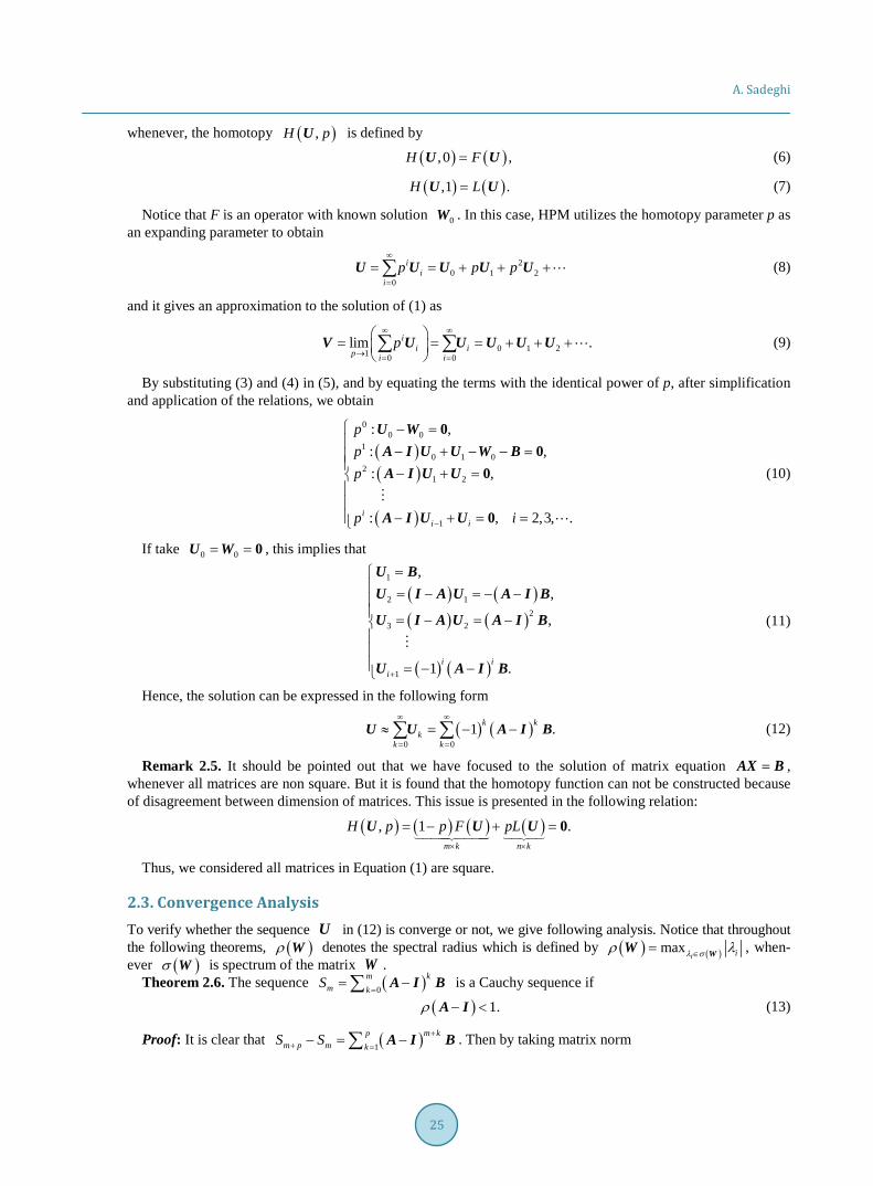
whenever, the homotopy ( ),H pU is defined by

( ) ( ),0 ,H F=U U (6)

( ) ( ),1 .H L=U U (7)

Notice that F is an operator with known solution 0W . In this case, HPM utilizes the homotopy parameter p as an expanding parameter to obtain

20 1 2

0

ii

ip p p

∞

=

= = + + +∑U U U U U (8)

and it gives an approximation to the solution of (1) as

0 1 21 0 0lim .i

i ip i ip

∞ ∞

→ = =

= = = + + + ∑ ∑ V U U U U U (9)

By substituting (3) and (4) in (5), and by equating the terms with the identical power of p, after simplification and application of the relations, we obtain

( )( )

( )

00 0

10 1 0

21 2

1

: ,: ,: ,

: , 2,3, .ii i

ppp

p i−

− =

− + − − =− + =

− + = =

U WA I U U W BA I U U

A I U U

00

0

0

(10)

If take 0 0= =U W 0 , this implies that

( ) ( )( ) ( )

( ) ( )

1

2 12

3 2

1

,,

,

1 .i ii+

= = − = − − = − = − = − −

U BU I A U A I B

U I A U A I B

U A I B

(11)

Hence, the solution can be expressed in the following form

( ) ( )0 0

1 .k kk

k k

∞ ∞

= =

≈ = − −∑ ∑U U A I B (12)

Remark 2.5. It should be pointed out that we have focused to the solution of matrix equation =AX B , whenever all matrices are non square. But it is found that the homotopy function can not be constructed because of disagreement between dimension of matrices. This issue is presented in the following relation:

( ) ( ) ( ) ( ), 1 .m k n k

H p p F pL× ×

= − + = 0

U U U

Thus, we considered all matrices in Equation (1) are square.

2.3. Convergence Analysis To verify whether the sequence U in (12) is converge or not, we give following analysis. Notice that throughout the following theorems, ( )ρ W denotes the spectral radius which is defined by ( ) ( )max

i iλ σρ λ∈= WW , when-ever ( )σ W is spectrum of the matrix W .

Theorem 2.6. The sequence ( )0km

m kS=

= −∑ A I B is a Cauchy sequence if

( ) 1.ρ − <A I (13)

Proof: It is clear that ( )1m kp

m p m kS S ++ =− = −∑ A I B . Then by taking matrix norm

A. Sadeghi

26

1

1 1

1 .1

pp pm k m k m

m p mk k

S S ξξ ξξ

+ + ++

= =

−− ≤ − = = −

∑ ∑B A I B B

Hence, if 1ξ = − <A I , we have obviously ( ) 1ρ − ≤A I , and then

lim 0.m p mmS S+→∞

− =

Thus nS is a Cauchy sequence. This completes theorem. Definition 2.7. [16] A matrix ijA a = is called strictly row diagonally dominant (SRDD), if we have

1,, 1, , .ii ij

j i ja a i n

= ≠

> =∑ (14)

Theorem 2.8. Consider the matrix 11

1 1diag , ,nnq q

=

Q where iiq are diagonal elements of matrix

1−B A . If the matrix 1−B A be SRDD, then we have

( )1 1.ρ − − <QB A I (15)

Proof: Suppose 1ijq− = B A and 1−= −M QB A I , then it can be easily shown that

0,

,ijij

ii

i jqm

i jq

= = − ≠

Since 1−B A is SRDD matrix, it is clear that 1,n

ii ijj j iq q= ≠

> ∑ . Hence,

1

1 1,1.

n nij

ijj j j i ii

qm

q−

∞ ∞= = ≠

= − = = <∑ ∑M QB A I

Therefore,

( ) 1,ρ∞

≤ <M M which completes the proof.

In Theorem 2.8, the important question is “Does the matrix 1−B A is SRDD whenever A and B are SRDD matrices?” The answer of this question is negative. Because, firstly the product of two SRDD matrices is

not SRDD, as a counterexample we can pay attention to the matrices 3 11 2

= − A and

0.5 0.41.0 3.0− −

= − − B ,

and their product is 2.5 4.2

1.5 5.6− −

=

AB . Secondly, inversion of SRDD matrix is not SRDD. As a counterex-

ample, consider 0.5 0.40.1 0.3

=

A which has the inversion 1 2.7 3.60.9 4.5

− − = −

A .

Now, if ( ) 1ρ − >I A , by pre-multiplying the both sides of Equation (1) by matrix Q , the following equa-tion can be obtain:

1 .− − =QB AX Q 0 (16)

To be more precise, by using convex homotopy function, we can easily verify that

( ) ( )11

01 .

nnn

n

∞−

+=

= − −∑U QB A I Q (17)

In this part, we would like to show that the series ( ) ( )10 1

iimm iS −

== − −∑ QB A I Q is converges. Thus, first

we need the following definition and theorems. Definition 2.9. [16] Let , ,A M N are three matrices satisfying = −A M N . The pair of matrices ,M N is

a regular splitting of A , if M is nonsingular and 1−M and N are nonnegative.

A. Sadeghi

27

Theorem 2.10. Let Q is nonsingular matrix such that Q and 1 1− −−Q B A are nonnegative. Then the se-quence

( ) ( )1

01

ii

i

∞−

=

= − −∑U I QB A Q (18)

converges if 1−B A is nonsingular and ( ) 11 −−B A is nonnegative. Proof: Suppose that Q is a singular matrix such that Q and 1 1− −−Q B A are nonnegative. By employing

Theorem 2.9 it can be obtain that ( )1 1ρ − − <QB A I as both Q and 1−−Q B A are a regular splitting of 1−B A . This implies that

( ) ( )1

01

m iim

iS Q−

=

= − −∑ QB A I (19)

is converges series.

3. Numerical Experiments In this section, some numerical illustrations are provided. All computations have been carried out using MATLAB 2012 (Ra) with roundoff error 1610u −≈ . Moreover, the error of the approximations have been measured by the following stopping criteria:

( ) 1010 ,−∞

∞

−= <

U XE U

X (20)

whereas, U is the approximated solution obtained by HPM. Example 3.1. First example made approximating the solution of the equation =AX B by using modified

HPM. In order to this purpose, two 4 4× matrices A and B are considered: 15.00 1.00 1.00 1.00 14.70 2.70 2.50 2.30

0 15.00 1.00 1.00 1.30 14.80 2.60 2.40, .

0 0 15.00 1.00 1.40 1.40 14.90 2.500 0 0 15.00 1.50 1.50 1.50 15.00

− − − − − − − − − − = = − −

A B

After evaluating the inversion of B and multiplying by A , it is observed that 1−B A is SRDD matrix, and

thus the matrix Q can be obtained as

( )11 22 33 44

1 1 1 1diag , , , diag 1.029,1.029,1.029,1.029 .q q q q

= =

Q

Furthermore, ( )1 0.13ρ −− =I QB A . Hence, considering seven terms of homotopy series as:

( ) ( )71 1 ,I − − ≈ + − + + − U I QB A I QB A Q

the approximated solution could be obtained as follows:

1.0000115 0.1000043 0.1000177 0.10002070.1000207 1.0000115 0.1000043 0.1000177

.0.1000177 0.1000207 1.0000115 0.10000430.1000043 0.1000177 0.1000207 1.0000115

− − − − − ≈ −

U

However, the exact solution of =AX B is

1 0.1 0.1 0.10.1 1 0.1 0.1

.0.1 0.1 1 0.10.1 0.1 0.1 1

− − − − − = −

X

In conclusion, it can be seen that the approximation has a good agreement with the exact solution. In this case

A. Sadeghi

28

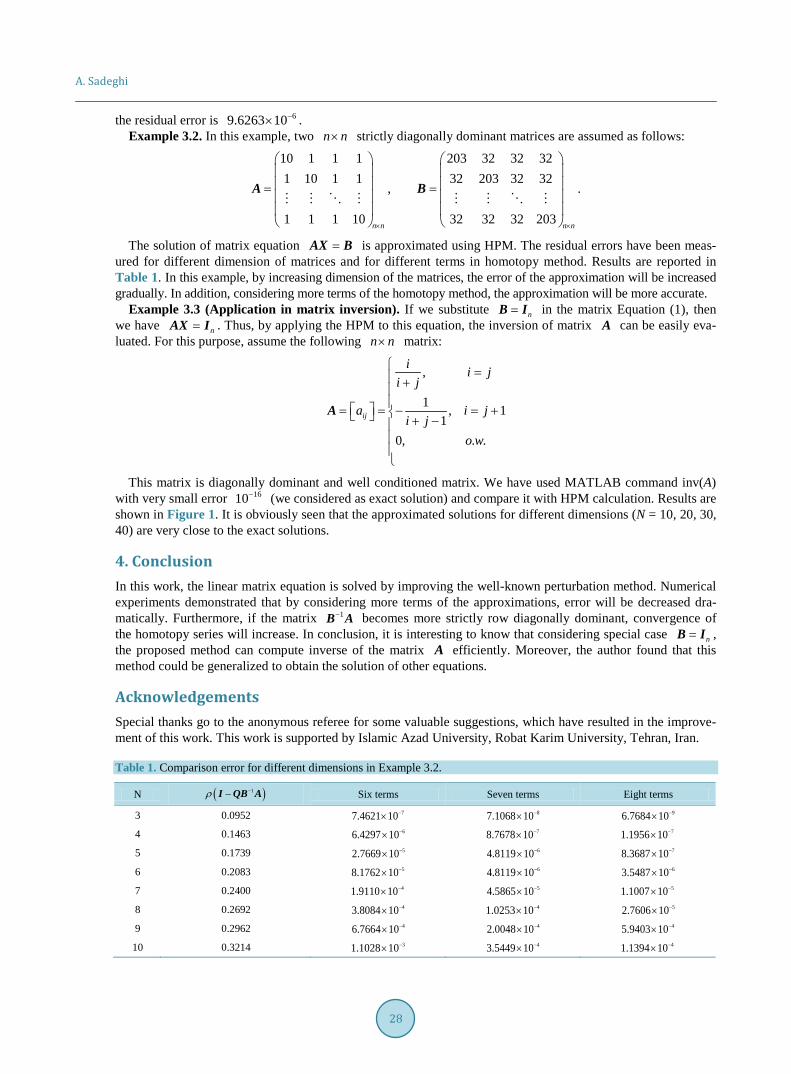
the residual error is 69.6263 10−× . Example 3.2. In this example, two n n× strictly diagonally dominant matrices are assumed as follows:

10 1 1 1 203 32 32 321 10 1 1 32 203 32 32

, .

1 1 1 10 32 32 32 203n n n n× ×

= =

A B

The solution of matrix equation =AX B is approximated using HPM. The residual errors have been meas-

ured for different dimension of matrices and for different terms in homotopy method. Results are reported in Table 1. In this example, by increasing dimension of the matrices, the error of the approximation will be increased gradually. In addition, considering more terms of the homotopy method, the approximation will be more accurate.

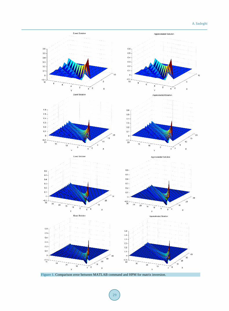
Example 3.3 (Application in matrix inversion). If we substitute n=B I in the matrix Equation (1), then we have n=AX I . Thus, by applying the HPM to this equation, the inversion of matrix A can be easily eva-luated. For this purpose, assume the following n n× matrix:

,

1 , 11

0, . .

ij

i i ji j

a i ji j

o w

= + = = − = + + −

A

This matrix is diagonally dominant and well conditioned matrix. We have used MATLAB command inv(A)

with very small error 1610− (we considered as exact solution) and compare it with HPM calculation. Results are shown in Figure 1. It is obviously seen that the approximated solutions for different dimensions (N = 10, 20, 30, 40) are very close to the exact solutions.

4. Conclusion In this work, the linear matrix equation is solved by improving the well-known perturbation method. Numerical experiments demonstrated that by considering more terms of the approximations, error will be decreased dra-matically. Furthermore, if the matrix 1−B A becomes more strictly row diagonally dominant, convergence of the homotopy series will increase. In conclusion, it is interesting to know that considering special case n=B I , the proposed method can compute inverse of the matrix A efficiently. Moreover, the author found that this method could be generalized to obtain the solution of other equations.

Acknowledgements Special thanks go to the anonymous referee for some valuable suggestions, which have resulted in the improve-ment of this work. This work is supported by Islamic Azad University, Robat Karim University, Tehran, Iran.

Table 1. Comparison error for different dimensions in Example 3.2.

N ( )1ρ −−I QB A Six terms Seven terms Eight terms

3 0.0952 77.4621 10−× 87.1068 10−×

96.7684 10−× 4 0.1463 66.4297 10−×

78.7678 10−× 71.1956 10−×

5 0.1739 52.7669 10−× 64.8119 10−×

78.3687 10−× 6 0.2083 58.1762 10−×

64.8119 10−× 63.5487 10−×

7 0.2400 41.9110 10−× 54.5865 10−×

51.1007 10−× 8 0.2692 43.8084 10−×

41.0253 10−× 52.7606 10−×

9 0.2962 46.7664 10−× 42.0048 10−×

45.9403 10−× 10 0.3214 31.1028 10−×

43.5449 10−× 41.1394 10−×

A. Sadeghi

29

Figure 1. Comparison error between MATLAB command and HPM for matrix inversion.

A. Sadeghi

30

Conflict of Interests The author declares that there is no conflict of interests regarding the publication of this article.

References [1] Bartels, R. and Stewart, G. (1994) Solution of the Matrix Equation AX XB C+ = . Circuits, Systems and Signal

Processing, 13, 820-826. [2] Benner, P. (2008) Large-Scale Matrix Equations of Special Type. Numerical Linear Algebra with Applications, 15,

747-754. http://dx.doi.org/10.1002/nla.621 [3] Golub, G., Nash, S. and Van Loan, Ch. (1979) A Hessenberg-Schur Method for the Problem AX XB C+ = . IEEE

Transactions on Automatic Control, 24, 909-913. http://dx.doi.org/10.1109/TAC.1979.1102170 [4] Sadeghi, A., Ahmad, M.I., Ahmad, A. and Abbasnejad, M.E. (2013) A Note on Solving the Fuzzy Sylvester Matrix

Equation. Journal of Computational Analysis and Applications, 15, 10-22. [5] Sadeghi, A., Abbasbandy, S. and Abbasnejad, M.E. (2011) The Common Solution of the Pair of Fuzzy Matrix Equa-

tions. World Applied Sciences, 15, 232-238. [6] Sadeghi, A., Abbasnejad, M.E. and Ahmad, M.I. (2011) On Solving Systems of Fuzzy Matrix Equation. Far East

Journal of Applied Mathematics, 59, 31-44. [7] He, J.H. (1999) Homotopy Perturbation Technique. Computer Methods in Applied Mechanics and Engineering, 57-62.

http://dx.doi.org/10.1016/s0045-7825(99)00018-3 [8] He, J.H. (2000) A Coupling Method of a Homotopy Technique and a Perturbation Technique for Non-Linear Problems.

International Journal of Non-Linear Mechanics, 35, 37-43. http://dx.doi.org/10.1016/S0020-7462(98)00085-7 [9] He, J.H. (2003) Homotopy Perturbation Method: A New Non-Linear Analytical Technique. Applied Mathematics and

Computation, 135, 73-79. http://dx.doi.org/10.1016/S0096-3003(01)00312-5 [10] Keramati, B. (2007) An Approach to the Solution of Linear System of Equations by He’s Homotopy Perturbation Me-

thod. Chaos, Solitons & Fractals, 41, 152-156. http://dx.doi.org/10.1016/j.chaos.2007.11.020 [11] Liu, H.K. (2011) Application of Homotopy Perturbation Methods for Solving Systems of Linear Equations. Applied

Mathematics and Computation, 217, 5259-5264. http://dx.doi.org/10.1016/j.amc.2010.11.024 [12] Edalatpanah, S.A. and Rashidi, M.M. (2014) On the Application of Homotopy Perturbation Method for Solving Sys-

tems of Linear Equations. International Scholarly Research Notices, 2014, Article ID: 143512. http://dx.doi.org/10.1155/2014/143512

[13] Saeidian, J., Babolian, E. and Aziz, A. (2015) On a Homotopy Based Method for Solving Systems of Linear Equations. TWMS Journal of Pure and Applied Mathematics, 6, 15-26.

[14] Khani, M.H., Rashidinia, J. and Zia Borujeni, S. (2015) Application of Different ( )H x in Homotopy Analysis Me-thods for Solving Systems of Linear Equations. Advances in Linear Algebra & Matrix Theory, 5, 129-137. http://dx.doi.org/10.4236/alamt.2015.53012

[15] Laub, A.J. (2005) Matrix Analysis for Scientists and Engineers. SIAM, Philadelphia. http://dx.doi.org/10.1137/1.9780898717907

[16] Saad, Y. (2003) Iterative Methods for Sparse Linear Systems. 2nd Edition, SIAM, Philadelphia. http://dx.doi.org/10.1137/1.9780898718003