A novel computer-aided lung nodule detection system for … · A novel computer-aided lung nodule detection system for CT images Maxine Tan Department of Electronics and Informatics

A novel computer-aided lung nodule detection system for CT images

Maxine TanDepartment of Electronics and Informatics (ETRO), Vrije Universiteit Brussel, Pleinlaan 2, B-1050 Brussel,Belgium

Rudi Deklerck and Bart JansenDepartment of Electronics and Informatics (ETRO), Vrije Universiteit Brussel, Pleinlaan 2, B-1050 Brussel,Belgium and Interdisciplinary Institute for Broadband Technology (IBBT), Gaston Crommenlaan 8,9050 Gent, Belgium

Michel Bister and Jan CornelisDepartment of Electronics and Informatics (ETRO), Vrije Universiteit Brussel, Pleinlaan 2, B-1050 Brussel,Belgium

(Received 24 February 2011; revised 16 August 2011; accepted for publication 17 August 2011;

published 22 September 2011)

Purpose: The paper presents a complete computer-aided detection (CAD) system for the detection

of lung nodules in computed tomography images. A new mixed feature selection and classificationmethodology is applied for the first time on a difficult medical image analysis problem.

Methods: The CAD system was trained and tested on images from the publicly available Lung

Image Database Consortium (LIDC) on the National Cancer Institute website. The detection stageof the system consists of a nodule segmentation method based on nodule and vessel enhancement

filters and a computed divergence feature to locate the centers of the nodule clusters. In the subse-

quent classification stage, invariant features, defined on a gauge coordinates system, are used to dif-

ferentiate between real nodules and some forms of blood vessels that are easily generating false

positive detections. The performance of the novel feature-selective classifier based on genetic algo-

rithms and artificial neural networks (ANNs) is compared with that of two other established classi-

fiers, namely, support vector machines (SVMs) and fixed-topology neural networks. A set of 235

randomly selected cases from the LIDC database was used to train the CAD system. The system

has been tested on 125 independent cases from the LIDC database.

Results: The overall performance of the fixed-topology ANN classifier slightly exceeds that of the

other classifiers, provided the number of internal ANN nodes is chosen well. Making educated

guesses about the number of internal ANN nodes is not needed in the new feature-selective classi-

fier, and therefore this classifier remains interesting due to its flexibility and adaptability to the com-

plexity of the classification problem to be solved. Our fixed-topology ANN classifier with 11

hidden nodes reaches a detection sensitivity of 87.5% with an average of four false positives per

scan, for nodules with diameter greater than or equal to 3 mm. Analysis of the false positive items

reveals that a considerable proportion (18%) of them are smaller nodules, less than 3 mm in

diameter.

Conclusions: A complete CAD system incorporating novel features is presented, and its perform-

ance with three separate classifiers is compared and analyzed. The overall performance of our CAD

system equipped with any of the three classifiers is well with respect to other methods described in

literature. VC 2011 American Association of Physicists in Medicine. [DOI: 10.1118/1.3633941]

Key words: medical image analysis, lung nodule detection, invariant image features, classifiers,

FD-NEAT

I. INTRODUCTION AND RELATED WORK

Several imaging modalities are used in recent work on com-

puterized methods for lung nodule detection and diagnosis,

e.g., for chest radiography1–3 and computed tomography

(CT) in both low-dose CT for screening purposes4–6 and

high resolution CT (HRCT).7–9 The increased interest in

lung nodule detection has resulted in the availability of pub-

lic image databases for the evaluation and validation of algo-

rithms. These include the Lung Image Database Consortium

(LIDC) image database,10 the ELCAP Public Lung Image

Database made available by Cornell University,11 and the

Lung TIME database.12 The “Automatic Nodule Detection

2009 (ANODE09)” database13 differs from the other data-

bases in that no ground truth data, annotations, markings are

provided (except in five cases): the images are used for test-

ing algorithms and comparisons with other systems.

The importance of developing automated methods is

underlined by statistics from the American Cancer Society;

in their most recent reports for the United States in 2009, it

is estimated that lung cancer will account for about 28% of

5630 Med. Phys. 38 (10), October 2011 0094-2405/2011/38(10)/5630/16/$30.00 VC 2011 Am. Assoc. Phys. Med. 5630

all cancer deaths, which is by far the leading cause of can-

cer death among both men and women.14 Early stage lung

cancer is typically manifested in the form of pulmonary

nodules, which are visible on CT scans as structures that

are roughly spherical in shape.

Various methods have been proposed to detect lung nodules

from clinical data. A few of these methods are briefly outlined

here. In Ref. 15, an automated method for lung nodule detec-

tion was developed based on grey-level-thresholding, using

rule-based classifiers and linear discriminant classifiers to dif-

ferentiate between nodule candidates resulting from the thresh-

olding process that correspond to actual nodules (or true

positives, TPs) and to nonnodules (false positives, FPs). In

Ref. 16, Paik et al. developed the surface normal overlap

method and applied it to colonic polyp detection and lung nod-

ule detection in CT images. Recently, Ye et al.17 combined vol-

umetric shape index and “dot” maps followed by adaptive

thresholding and modified expectation-maximization methods

to segment potential nodule objects. For the classification stage,

the authors use rule-based filtering methods followed by a

weighted support vector machine (SVM) classification.

In early work by Lee et al.,18 template-matching was pro-

posed based on genetic algorithms (GAs) and using rule-

based methods to remove FPs. Boroczky et al.19 present a

feature subset selection method based on GAs coupled with

an SVM classifier to reduce the FPs generated by a lung nod-

ule detection unit.8 The use of a massive training artificial

neural network (MTANN) to enhance nodules and suppress

vessels and to distinguish between benign and malignant

nodules is explored in Refs. 20–23. The method is shown to

have potential in distinguishing between nodules and vessels

and in reducing the number of FPs in a lung nodule detection

scheme.

Brown et al.24 describe a method based on anatomical mod-

eling using fuzzy sets. An example-based approach to help in

classifying nodules is proposed by Kawata et al.25 In Ref. 26,

Golosio et al. use multithreshold surface-triangulation and

computed features provided to a fixed-topology artificial neural

network (ANN) for nodule detection in lung CT. In Ref. 27,

Suarez-Cuenca et al. investigate the capability of an iris filter to

discriminate between nodules and false positives, and they

evaluate their system on CT scans containing 77 nodules in

total. Retico et al. propose a method to automatically detect

subpleural nodules in Ref. 28, and they validate their method

on a dataset of 42 annotated CT scans. In Ref. 29, Li et al.apply a selective nodule enhancement filter to considerably

enhance nodules and suppress blood vessels and an automated

rule-based classifier to reduce FPs on a database of 117 thin-

section CT scans with 153 nodules. Performance analysis of

computer-aided detection (CAD) systems on datasets annotated

by multiple radiologists are reported by Sahiner et al.30 and

Opfer and Wiemker.31

A CAD system for lung nodule detection based on inten-

sity thresholding, morphological processing, and linear dis-

criminant and quadratic classifiers is validated on the LIDC

and ANODE09 databases in a paper by Messay et al.32 In

Ref. 33, Ge et al. propose the use of some three-dimensional

(3D) gradient field descriptors and ellipsoid features to

reduce the number of FPs in a CAD system for lung nodule

detection in CT images. Pu et al.34 present a simple compu-

terized scheme for lung nodule detection based on geometric

analysis of a signed distance field, and they test their method

on 52 low-dose screening CT scans with 184 nodules alto-

gether, including part-solid and nonsolid nodules. In Ref. 35,

Zhang et al. propose a novel method called local shape con-

trolled voting that improves on the normal overlap method

proposed by Paik.16 The authors validate their method on 42

HRCT cases and show that better performance is obtained

compared to the original method with improved time effi-

ciency. For a more complete overview of computerized

methods that have been developed for the lungs, the reader

is referred to several literature reviews=surveys.36–38

In the field of lung nodule detection, many of the devel-

oped methods propose optimal feature selection techniques

before the classification stage.5,19,32 Hence, feature selection

and classification appear as two separate stages in the CAD

system. In this paper, a new feature-selective classifier is

briefly described, “Feature-Deselective Neuro-Evolving

Augmenting of Topologies (FD-NEAT),” and applied for

the first time on a complex image analysis problem. The

behavior of FD-NEAT was previously examined on several

simple feature-selective experiments,39 e.g., the classical

exclusive or classification problem and maneuvering a

robotic car around a race track by selecting relevant sensors

in a race car simulator environment (RARS).40 The novelty

of FD-NEAT is the incorporation of the feature selection

into the classification task.39 In general, low complexity net-

works are obtained (either with a lower number of internal

nodes or connections or both) that can be trained faster and

are computationally less expensive in the operational phase.

FD-NEAT is based on the NEAT method proposed by Stan-

ley et al.41 With NEAT, the topology of the ANN does not

have to be predefined. FD-NEAT extends the NEAT method

to feature selection, namely, FD-NEAT selects relevant fea-

tures at the same time as it determines the topology of the

network that best solves the classification task. The opera-

tional principles behind NEAT and FD-NEAT are described

in some more detail in Sec. III.

New is also the use of the “divergence of the normalized

gradient or mean curvature feature in 3D” in the detection

stage of the CAD system. In the detection stage, separate

schemes are derived for different nodule types, namely, for

the isolated, juxtavascular (or vessel-connected), and juxta-

pleural (or pleura-connected) nodules. The differential invar-

iants used in the nodule detection algorithm are based on the

method proposed by Salden et al.42 in 3D and by Romeny in

2D.43 The invariant features are computed after fixing a

gauge coordinate system to the image topology.

The outline of the paper is as follows: first, the datasets

used in our experiments are described in Sec. II. Section III

starts with the Preprocessing including isotropic re-sampling

of the lung images and the lung segmentation algorithm, fol-

lowed by the Nodule Candidate Detection including the

extraction methods for suspicious lung nodule candidates

from within the segmented lungs and for different nodule

5631 Tan et al.: Novel CAD system for CT lung nodule detection 5631

Medical Physics, Vol. 38, No. 10, October 2011

types, namely, for the isolated, juxtavascular, and juxtapleu-

ral (or subpleural) nodules. Section III C. contains a detailed

description of the features and classifiers that are analyzed in

our experiments. Section IV is about experimental results

followed by Secs. V and VI on discussion and conclusions,

respectively.

II. MATERIALS

Our CAD system was trained and tested on lung images

made publicly available by the Lung Image Database Consor-

tium (LIDC). Following the rule of thumb that is usually

applied for splitting a data set in a training and independent

test set––approximately 2=3 versus 1=3 of the cases––we have

chosen to include in the training set 235 CT scans and in the

test set 125 scans.19,27 Currently, as of December 2010, there

are 399 scans that can be downloaded from the website of the

National Biomedical Imaging Archive (NBIA) of the National

Cancer Institute (NCI). Specific details about the cases used

for training and testing are provided in Appendix A, as well

as a motivated list of cases excluded from this research. The

LIDC database is the result of a cooperative effort between

five academic institutions in the US to develop an image data-

base as a web-accessible international research resource for

the development, training, evaluation, and comparison of

CAD methods and algorithms for lung cancer detection and

diagnosis in helical CT. A range of scanner manufacturers

and models are represented in the database.10,44

Each scan is provided with annotations by four experi-

enced radiologists (each from a different institution), who

drew complete outlines and identified the radiological charac-

teristics of all nodules between 3 and 30 mm in diameter in

the scans. The 3D center-of-mass of non-nodules=anomalies

larger than 3 mm in diameter and nodules less than 3 mm

were also marked by the radiologists. A “blinded” and

“unblinded” reviewing procedure was established. In the

blinded review stage, each radiologist individually marked the

nodules=lesions in a blinded fashion. In the unblinded review,

each radiologist re-examined the cases with the additional in-

formation of the markings of the other radiologists. No forced

consensus was imposed in the final review.

With the data compiled by LIDC, a study can be per-

formed taking into account the agreement levels between the

four radiologists, for different nodule types, before and after

the unblinded read session.45,46 There are various ways of

building a reference standard based on the annotations of the

four radiologists. In this paper, we used the method

employed in Refs. 26 and 31 called ground truth with agree-ment level j; the list of all the nodules marked by at least j of

the four radiologists (Annotations smaller than 600 mm3

with centroids within a distance of 5 mm are considered the

same nodule. For annotations bigger than 600 mm3 a thresh-

old of 9 mm is used. See Sec. IV where we use the same cri-

teria for defining the scoring rules). In general, it is desirable

to obtain higher sensitivities for nodules identified with

higher agreement levels. CAD system performance evalua-

tion studies using the LIDC database have been conducted

by Opfer and Wiemker,31 Golosio et al.,26 and Messay

et al.32 among others.

III. METHODS

The CAD system performs four main tasks: preprocess-

ing, nodule candidate detection, feature selection, and classi-

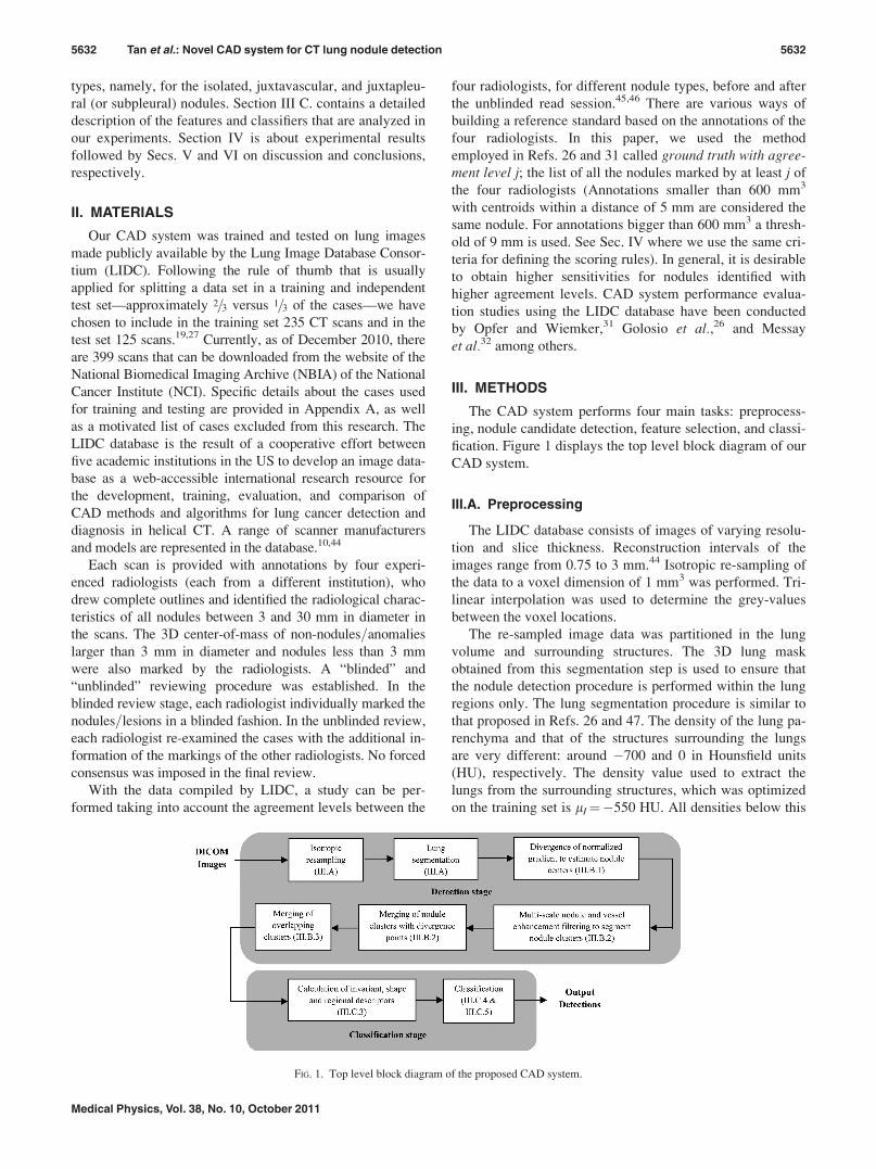
fication. Figure 1 displays the top level block diagram of our

CAD system.

III.A. Preprocessing

The LIDC database consists of images of varying resolu-

tion and slice thickness. Reconstruction intervals of the

images range from 0.75 to 3 mm.44 Isotropic re-sampling of

the data to a voxel dimension of 1 mm3 was performed. Tri-

linear interpolation was used to determine the grey-values

between the voxel locations.

The re-sampled image data was partitioned in the lung

volume and surrounding structures. The 3D lung mask

obtained from this segmentation step is used to ensure that

the nodule detection procedure is performed within the lung

regions only. The lung segmentation procedure is similar to

that proposed in Refs. 26 and 47. The density of the lung pa-

renchyma and that of the structures surrounding the lungs

are very different: around �700 and 0 in Hounsfield units

(HU), respectively. The density value used to extract the

lungs from the surrounding structures, which was optimized

on the training set is lI¼�550 HU. All densities below this

FIG. 1. Top level block diagram of the proposed CAD system.



threshold are retained as foreground. From this foreground,

we remove the segments touching the upper and lower image

borders and the segments adjacent to the lower halves of the

left and right image borders. In our method, the lungs region

of interest (ROI) is then obtained by extracting the largest

foreground segment. In most cases, this approach works

well, as the two lungs are extracted as one segment, since in

3D there is a connection through the primary bronchi and in

several transversal slices both lungs are very close to each

other. However, in some cases where pathology is present,

two segments are obtained. This is detected automatically: if

the second largest segment contains more than half of the

number of voxels of the largest one, then both segments are

considered as the lungs ROI.

A 3-D morphological closing operation using a “ball”

structuring element of radius 13 voxels is then applied to the

parenchyma mask to include missing structures within the

lungs and juxtapleural nodules, i.e., nodules connected to the

pleural surface.

III.B. Nodule candidate detection

Three different types of nodules are considered, namely,

isolated, juxtavascular (or vessel-connected), and juxtapleu-

ral (or pleura-connected) nodules. Due to inherent differen-

ces in their nature and appearance in the images, we derive

specific segmentation algorithms with different parameter

settings for each nodule type.

Our nodule segmentation method uses selective nodule

and vessel enhancement filters presented by Li et al.48,49

These filters have been explored extensively and analyzed

with other methods in several publications.17,29,50 The main

problem of using these nodule enhancement filters is the

high amount of FP detections, especially in the locations of

vessel branches and junctions. To better estimate the loca-

tion of the nodule centers and to reduce the FP rate, we use

the maxima of the divergence of the normalized gradient of

the image in 3D to generate seed points (see Sec. III B 1).

The nodule centers are subsequently merged with the seg-

mented nodule clusters (see Sec. III B 2). Finally, a cluster

merging stage is implemented to cluster overlapping nodules

and to reduce the number of FPs (see Sec. III B 3).

III.B.1. Seed point detection by divergence ofnormalized gradient (DNG)

To determine the seed point of the nodule, we use the

divergence of the normalized gradient of the image in 3D

k ¼ divð~wÞ, where ~w ¼ ~rL=k ~rL k and L is the image in-

tensity. The DNG is equivalent to the mean curvature in 3D.

Hereafter, we explain that the maxima of the divergence

yield a good estimate of the locations of the nodule seed

points or centers. In general, the divergence is an operator

that measures the magnitude of a vector field’s source or

sink at a given point. It is a signed scalar representing the

volume density of the outward flux of a vector field from an

infinitesimal volume around that point.

In the context of our application, a lung nodule can be

modeled as a sphere with decreasing intensity along the ra-

dial axis against a darker background. The div operator is

applied on the normalized image intensity gradient vector

field. Many partial derivatives of the image must be com-

puted in the divergence calculation. To reduce the noise sen-

sitivity, the original image is blurred with a Gaussian prior

to the application of the div operator. The location corre-

sponding to the maximum of the DNG in the region of a

nodule is a good estimate of the center or seed point of that

nodule.

In order to detect the seed points of different-sized nod-

ules, the maxima of the DNG are computed at multiple

scales taken from a set of 6 scales r, ranging from 1 to 4

mm. The maxima, which correspond to values above thresh-

old 100 for isolated=juxtavascular nodules and above thresh-

old 25 for juxtapleural nodules are retained as seed points.

The threshold values are determined experimentally and are

maintained at each scale. A maximum response of the diver-

gence filter is obtained when the width of the Gaussian ker-

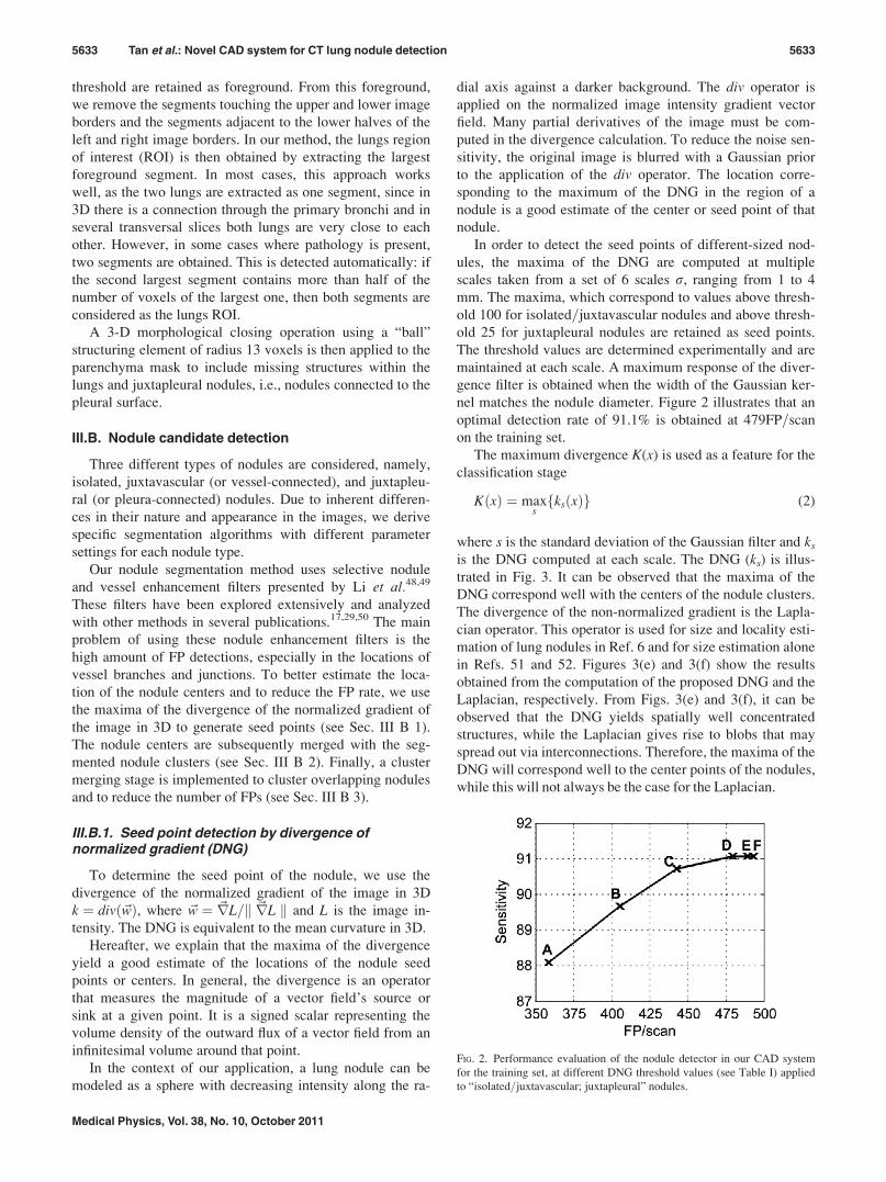
nel matches the nodule diameter. Figure 2 illustrates that an

optimal detection rate of 91.1% is obtained at 479FP=scan

on the training set.

The maximum divergence K(x) is used as a feature for the

classification stage

KðxÞ ¼ maxsfksðxÞg (2)

where s is the standard deviation of the Gaussian filter and ks

is the DNG computed at each scale. The DNG (ks) is illus-

trated in Fig. 3. It can be observed that the maxima of the

DNG correspond well with the centers of the nodule clusters.

The divergence of the non-normalized gradient is the Lapla-

cian operator. This operator is used for size and locality esti-

mation of lung nodules in Ref. 6 and for size estimation alone

in Refs. 51 and 52. Figures 3(e) and 3(f) show the results

obtained from the computation of the proposed DNG and the

Laplacian, respectively. From Figs. 3(e) and 3(f), it can be

observed that the DNG yields spatially well concentrated

structures, while the Laplacian gives rise to blobs that may

spread out via interconnections. Therefore, the maxima of the

DNG will correspond well to the center points of the nodules,

while this will not always be the case for the Laplacian.

FIG. 2. Performance evaluation of the nodule detector in our CAD system

for the training set, at different DNG threshold values (see Table I) applied

to “isolated=juxtavascular; juxtapleural” nodules.



Computing the DNG is just the first step of our proposed

nodule segmentation procedure. The maxima of the DNG

merely give an estimate of the locations of the nodule cen-

ters. To segment the nodule candidates, we use nodule and

vessel enhancement filters proposed by Li et al.48,49 These

filters have also been used for nodule detection in Refs. 17

and 53. The nodules are segmented by thresholding

the nodule-filtered image; different thresholds are used

for isolated=juxtavascular and juxtapleural nodules (see

Sec. III B 2).

III.B.2. Multiscale nodule and vessel enhancementfiltering

In Ref. 48, Li et al. propose the use of a nodule

enhancement filter and a vessel enhancement filter to seg-

ment nodules and vessels, respectively. In our experi-

ments, the nodule and vessel enhancement filters are

calculated at six different scales in a range of 1–4 mm. A

thresholding step is implemented on the nodule-enhanced

image to form clusters or voxels of interest. The thresh-

olds are determined empirically and differ for juxtapleural

and isolated=juxtavascular nodules. Also the voxel-

clustering procedure itself is different for the different

nodule types.

To extract the candidate isolated nodules, we perform a

threshold operation at �600 HU on the re-sampled image

within the region defined by the lung mask region obtained

as described in Sec. III A. A grey-level threshold value of

6 is subsequently applied on the nodule-enhanced image.

Resulting clusters that have values above the threshold are

confronted with the DNG seed points extracted in the previ-

ous stage: the clusters that correspond to those seed points

and whose volumes are more than tvol are kept as possible

isolated nodule candidates. During the development stage of

the system, tvol was empirically set at 9 voxels for isolated

and juxtavascular nodule candidates. To reject huge struc-

tures within the isolated nodule candidates set such as

branching blood vessels and structures that are erroneously

included in the lung mask, a threshold on the maximum size

of the candidates is set to 500 voxels. Note that low values

of tvol can be used, because the calculation of features for the

classification stage is performed on larger spherical kernels

to enhance the robustness (see also Sec. III C 3).

The juxtavascular nodule detection is applied on the nod-

ules that were omitted from the isolated nodule detection

stage due to connections or linkages with blood vessels or

other structures. An empirically determined threshold of 150

is applied on the vessel-enhanced image. The points corre-

sponding to maxima of the DNG within the thresholded

vessel-enhanced image are more likely to be vessel junctions

or branches and are omitted too. The remaining maxima of

the DNG are used as seed points in a 3D constrained region

growing performed on the nodule-enhanced images. For

each juxtavascular nodule candidate, the seed point is a max-

imum of the DNG, which falls within a distance of 2 voxels

from the nodule cluster. The region growing is limited to 30

voxels. Voxels are added to the seed region if (i) these vox-

els are adjacent to (in terms of the 26-neighbourhood in 3D

TABLE I. Specific divergence threshold values applied to isolated=juxtavas-

cular nodules (divvals) and to juxtapleural nodules (divjux) at the points on

the graph displayed in Fig. 2.

Point

Divergence threshold applied to

isolated=juxtavascular

nodules (divvals)

Divergence threshold

applied to juxtapleural

nodules (divjux)

A 400 125

B 300 75

C 200 50

D 100 25

E 50 15

F 30 8

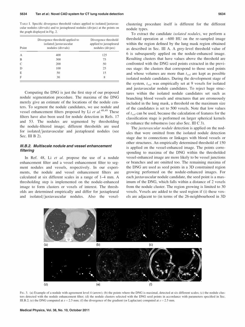
FIG. 3. (a) Example of a nodule with agreement level 4 (arrow); (b) the points where the DNG is maximal, detected at six different scales; (c) the nodule clus-

ters detected with the nodule enhancement filter; (d) the nodule clusters selected with the DNG seed points in accordance with parameters specified in Sec.

III.B.2; (e) the DNG computed at s¼ 2.5 mm; (f) the divergence of the gradient (or Laplacian) computed at s¼ 2.5 mm.



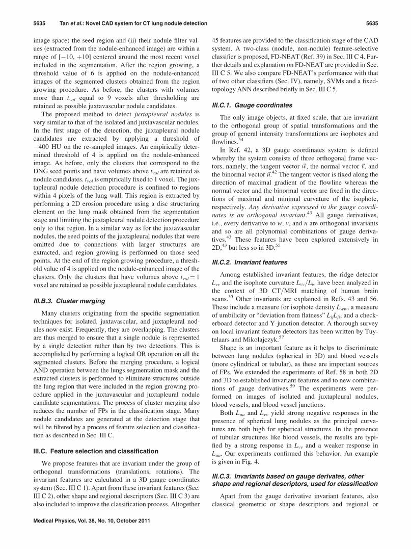
image space) the seed region and (ii) their nodule filter val-

ues (extracted from the nodule-enhanced image) are within a

range of [�10, þ10] centered around the most recent voxel

included in the segmentation. After the region growing, a

threshold value of 6 is applied on the nodule-enhanced

images of the segmented clusters obtained from the region

growing procedure. As before, the clusters with volumes

more than tvol equal to 9 voxels after thresholding are

retained as possible juxtavascular nodule candidates.

The proposed method to detect juxtapleural nodules is

very similar to that of the isolated and juxtavascular nodules.

In the first stage of the detection, the juxtapleural nodule

candidates are extracted by applying a threshold of

�400 HU on the re-sampled images. An empirically deter-

mined threshold of 4 is applied on the nodule-enhanced

image. As before, only the clusters that correspond to the

DNG seed points and have volumes above tvol are retained as

nodule candidates. tvol is empirically fixed to 1 voxel. The jux-

tapleural nodule detection procedure is confined to regions

within 4 pixels of the lung wall. This region is extracted by

performing a 2D erosion procedure using a disc structuring

element on the lung mask obtained from the segmentation

stage and limiting the juxtapleural nodule detection procedure

only to that region. In a similar way as for the juxtavascular

nodules, the seed points of the juxtapleural nodules that were

omitted due to connections with larger structures are

extracted, and region growing is performed on those seed

points. At the end of the region growing procedure, a thresh-

old value of 4 is applied on the nodule-enhanced image of the

clusters. Only the clusters that have volumes above tvol¼ 1

voxel are retained as possible juxtapleural nodule candidates.

III.B.3. Cluster merging

Many clusters originating from the specific segmentation

techniques for isolated, juxtavascular, and juxtapleural nod-

ules now exist. Frequently, they are overlapping. The clusters

are thus merged to ensure that a single nodule is represented

by a single detection rather than by two detections. This is

accomplished by performing a logical OR operation on all the

segmented clusters. Before the merging procedure, a logical

AND operation between the lungs segmentation mask and the

extracted clusters is performed to eliminate structures outside

the lung region that were included in the region growing pro-

cedure applied in the juxtavascular and juxtapleural nodule

candidate segmentations. The process of cluster merging also

reduces the number of FPs in the classification stage. Many

nodule candidates are generated at the detection stage that

will be filtered by a process of feature selection and classifica-

tion as described in Sec. III C.

III.C. Feature selection and classification

We propose features that are invariant under the group of

orthogonal transformations (translations, rotations). The

invariant features are calculated in a 3D gauge coordinates

system (Sec. III C 1). Apart from these invariant features (Sec.

III C 2), other shape and regional descriptors (Sec. III C 3) are

also included to improve the classification process. Altogether

45 features are provided to the classification stage of the CAD

system. A two-class (nodule, non-nodule) feature-selective

classifier is proposed, FD-NEAT (Ref. 39) in Sec. III C 4. Fur-

ther details and explanation on FD-NEAT are provided in Sec.

III C 5. We also compare FD-NEAT’s performance with that

of two other classifiers (Sec. IV), namely, SVMs and a fixed-

topology ANN described briefly in Sec. III C 5.

III.C.1. Gauge coordinates

The only image objects, at fixed scale, that are invariant

to the orthogonal group of spatial transformations and the

group of general intensity transformations are isophotes and

flowlines.54

In Ref. 42, a 3D gauge coordinates system is defined

whereby the system consists of three orthogonal frame vec-

tors, namely, the tangent vector ~w, the normal vector ~v, and

the binormal vector ~u.42 The tangent vector is fixed along the

direction of maximal gradient of the flowline whereas the

normal vector and the binormal vector are fixed in the direc-

tions of maximal and minimal curvature of the isophote,

respectively. Any derivative expressed in the gauge coordi-nates is an orthogonal invariant.43 All gauge derivatives,

i.e., every derivative to w, v, and u are orthogonal invariants

and so are all polynomial combinations of gauge deriva-

tives.43 These features have been explored extensively in

2D,43 but less so in 3D.55

III.C.2. Invariant features

Among established invariant features, the ridge detector

Lvv and the isophote curvature Lvv=Lw have been analyzed in

the context of 3D CT=MRI matching of human brain

scans.55 Other invariants are explained in Refs. 43 and 56.

These include a measure for isophote density Lww, a measure

of umbilicity or “deviation from flatness” LijLji, and a check-

erboard detector and Y-junction detector. A thorough survey

on local invariant feature detectors has been written by Tuy-

telaars and Mikolajczyk.57

Shape is an important feature as it helps to discriminate

between lung nodules (spherical in 3D) and blood vessels

(more cylindrical or tubular), as these are important sources

of FPs. We extended the experiments of Ref. 58 in both 2D

and 3D to established invariant features and to new combina-

tions of gauge derivatives.59 The experiments were per-

formed on images of isolated and juxtapleural nodules,

blood vessels, and blood vessel junctions.

Both Luu and Lvv yield strong negative responses in the

presence of spherical lung nodules as the principal curva-

tures are both high for spherical structures. In the presence

of tubular structures like blood vessels, the results are typi-

fied by a strong response in Lvv and a weaker response in

Luu. Our experiments confirmed this behavior. An example

is given in Fig. 4.

III.C.3. Invariants based on gauge derivates, othershape and regional descriptors, used for classification

Apart from the gauge derivative invariant features, also

classical geometric or shape descriptors and regional or



grey-value descriptors are computed for the classification. A

list is given in Table II.

Luu and Lvv are computed on the candidate nodule seg-

mentations and on spherical kernels of radii 1 and 3 pixels

(or 1 and 3 mm) centered at the centroids of the nodule can-

didates at scales, s¼ 1 and 2 pixels. The mean nodule filter

output, the mean vessel filter output, and the mean K(x)

defined in Eq. (2) are computed for each nodule candidate

and for two spherical kernels (of 1 and 3 mm) centered at the

nodule candidate centroids. The main purpose for computing

the features on spherical kernels is that in some cases the

nodule candidates consist of only a few pixels as a result of

applying a threshold on the nodule filter in the detection

stage. In these cases, computation of the features on only a

few pixels might not be truly representative of the features

of the nodule or structure in question. Also, the gauge coor-

dinates are not defined at singular points in the intensity

landscape.43 In Ref. 5, the authors compute some grey-value

features over spherical kernels to eliminate structures that do

not lie in sufficiently bright regions.

III.C.4. A feature-selective classifier based on ANNsand genetic algorithms (FD-NEAT)

The optimal ANN topology and complexity are often

unknown, and therefore heuristically chosen. Since the

ANN topology determines the size of the search space, the

consequences of wrong choices could be severe. Searching

in too large a space is intractable whereas searching in too

small a space limits solution quality. The network complex-

ity also determines how fast a solution is found. The addi-

tion of every extraneous feature adds at least one dimension

to the search space. However, if important features are

excluded, it might be impossible to find an optimal solution.

These problems highlight the need for feature selection

algorithms, and the need to find optimal solutions in sim-

pler structures.

Neuroevolution is a form of machine learning that uses

GAs to evolve ANNs. With NEAT,41 a designer is not

required to propose a network topology in advance; NEAT

automatically discovers the topology and weights of the net-

work that best fits the complexity of the task at hand. In

NEAT, evolution starts from an almost minimal structure

with all the inputs connected directly to all the outputs. New

structure is added incrementally through the mutation

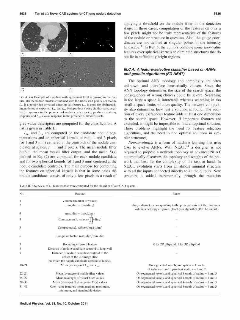
FIG. 4. (a) Example of a nodule with agreement level 4 (arrow) in the pic-

ture; (b) the nodule clusters combined with the DNG seed points; (c) feature

Lvv is a good ridge or vessel detector; (d) feature Luu is good for distinguish-

ing nodules; as expected, Luu and Lvv both produce strong (in this case, nega-

tive) responses in the presence of nodules whereas Lvv produces a strong

response and Luu a weak response in the presence of blood vessels.

TABLE II. Overview of all features that were computed for the classifier of our CAD system.

No. Feature Notes

1 Volume (number of voxels)

2 min_dim¼mini(dimi) dimi¼ diameter corresponding to the principal axis i of the minimum

volume-enclosing ellipsoid, (Kachiyan algorithm (Ref. 60 and 61)

3 max_dim¼maxi(dimi) –

4 Compactness1, volume=Y3

i¼1

ðdimiÞ –

5 Compactness2, volume=max dim3 –

6 Elongation factor, max dim=min dim –

7 Bounding ellipsoid feature 0 for 2D ellipsoid; 1 for 3D ellipsoid

8 Distance of nodule candidate centroid to lung wall –

9 Distance of nodule candidate centroid to the

center of the 2D image slice

on which the nodule candidate centroid is located

–

10–21 Mean (average) of Luu and Lvv On segmented voxels, and spherical kernels

of radius¼ 1 and 3 pixels at scale, s¼ 1 and 2

22–24 Mean (average) of nodule filter values On segmented voxels, and spherical kernels of radius¼ 1 and 3

25–27 Mean (average) of vessel filter values On segmented voxels, and spherical kernels of radius¼ 1 and 3

28–30 Mean (average) of divergence K (x) values On segmented voxels, and spherical kernels of radius¼ 1 and 3

31–45 Grey-value features: mean, median, maximum,

minimum, and standard deviation

On segmented voxels, and spherical kernels of radius¼ 1 and 3



operators. Starting minimally helps NEAT to learn fast as it

searches for an optimal solution over a lower-dimensional

search space. NEAT only jumps to a larger search space

when performance in the smaller one stagnates (i.e., does not

improve over a specified number of generations). Since only

additional structures that improve performance are likely to

be retained, NEAT tends to discover small networks without

superfluous or unnecessary structures.

In regular NEAT all the initial inputs are considered to be

relevant or useful to the network’s performance. When it is

not certain that all inputs are relevant, the initial connections

of NEAT might impair the performance of the search algo-

rithm as the search space is increased by the high number of

initial input connections.

A feature-selective version of NEAT, namely, FS-NEAT,

is presented by Whiteson et al.62,63 FS-NEAT is an extension

to NEAT that attempts to solve the feature selection problem

by starting even more minimally than NEAT, namely, with

networks having only one randomly selected input connected

to a randomly selected output in the initial network popula-

tion. However, in most tasks, FS-NEAT’s networks lack the

necessary structure to perform well.39,64

Recently, a novel feature-selective version of NEAT,

namely, FD-NEAT,39 was presented. As opposed to FS-

NEAT, FD-NEAT starts in the same way as regular NEAT,

with all inputs connected to all the outputs. However, with

FD-NEAT, an additional mutation operator enables discard-

ing irrelevant or redundant inputs. Hence, FD-NEAT prunes

the input features in the initial set instead of adding features.

FD-NEAT is able to optimize its weights quickly so that

suitable weights can be assigned to features based on their

relevance or redundancy. FD-NEAT is shown to outperform

FS-NEAT on a number of feature-selective tasks.39

III.C.5. Performance comparisons with otherclassifiers

FD-NEAT’s performance is compared with that of two

other established classifiers, namely, SVMs and fixed-

topology ANNs. All results are obtained for a test set that is

kept completely separated from the training set.

A LIBSVM (Ref. 65) classifier with the radial basis func-

tion (RBF) kernel defined as Kðxi; xjÞ ¼ expð�ckxi � xjk2Þ,c> 0 is designed on a training set of instance-label pairs

(xi, yi), i¼ 1, …, l where xi 2 Rn and y 2 f1;�1gl. Five-fold

cross-validation with parallel “grid-search”66 is used to

determine the penalty parameter of the error term and c. In

our approach, we perform linear normalization of all input

features.

The second classifier is the standard feed-forward ANNhaving a single hidden layer with hyperbolic tangent activa-

tion function at the hidden nodes, and linear transfer function

at the output node. The number of input nodes is equal to the

number of features, i.e., 45. Only one output node is used;

values at the output node above a certain threshold depend-

ing on the FP rate correspond to nodule detections and val-

ues below to non-nodule detections. The fixed-topology ANNis trained through the Levenberg-Marquardt backpropaga-

tion algorithm.67,68 The network’s performance is analyzed

for 5–40 neurons in the hidden layer, which is always initial-

ized with random weights.

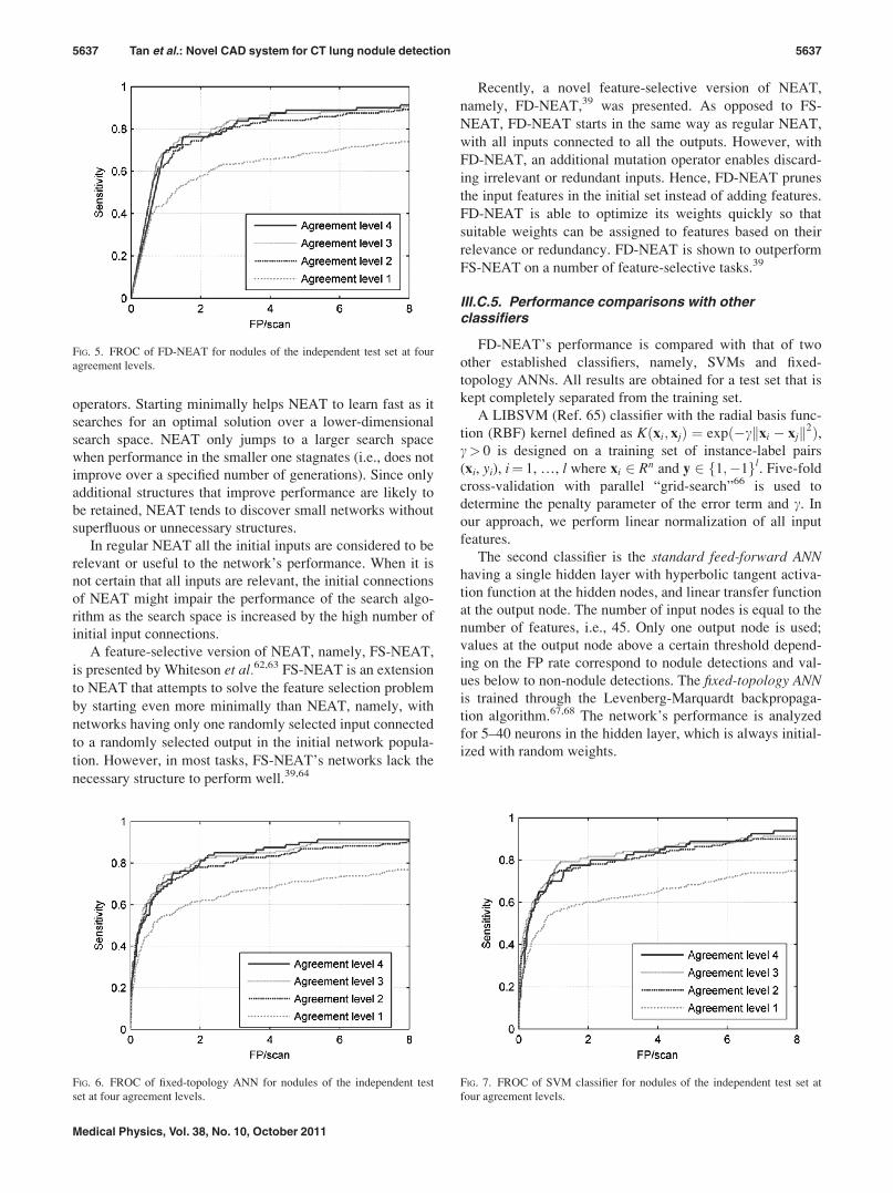
FIG. 5. FROC of FD-NEAT for nodules of the independent test set at four

agreement levels.

FIG. 6. FROC of fixed-topology ANN for nodules of the independent test

set at four agreement levels.

FIG. 7. FROC of SVM classifier for nodules of the independent test set at

four agreement levels.



For FD-NEAT, the hyperbolic tangent activation func-

tion is used at the hidden nodes whereas a modified

sigmoidal transfer function is implemented at the output

node. Experiments show that FD-NEAT performs better

when the modified sigmoidal transfer function instead

of the linear transfer function, is used at the output

node.

FD-NEAT and the fixed-topology ANN (The fixed-

topology ANN performs best with 11 neurons in the hidden

layer) are trained on a target vector with different values

(0.55, 0.7, 0.85, and 1) assigned to nodules at different

agreement levels, while SVM is trained on a target vector

in which the same target value is used for all agreement

levels. This strategy was based on initial experimental

results showing optimal performance under these learning

strategies.

FD-NEAT is found to perform best when the variance

normalization (normalization of the mean and standard devi-

ation of the training set) is applied to the input features

whereas the SVM and fixed-topology ANN perform better

when the features are normalized linearly.

III.C.6. Classification methodology and experimentalsetup

The number of detections is very large on the training data-

set of 235 CT scans (just after the detection stage, see Fig. 1):

111 906 detections altogether. The nodules having a diameter

between 3 to 30 mm (574 in total) that are identified by

different radiologists are divided into four subsets, with the

number of nodules equal to 202=113=104=155 nodules anno-

tated by 1=2=3=4 radiologists, respectively.

There are altogether 111 332 non-nodule regions in the

training set generated by the detection stage of our CAD sys-

tem, i.e., an average of 474 non-nodules per scan. The train-

ing and validation procedure does not work if there are too

many negative examples (i.e., non-nodule regions) compared

to positive ones. Hence, it is important to reduce the number

of non-nodule regions without altering their distribution in

the feature space. A possible way of doing this is by using a

2D selforganizing map (SOM).69–71

At the end of the unsupervised learning procedure, based

on the winner-takes-all rule, the non-nodule regions are

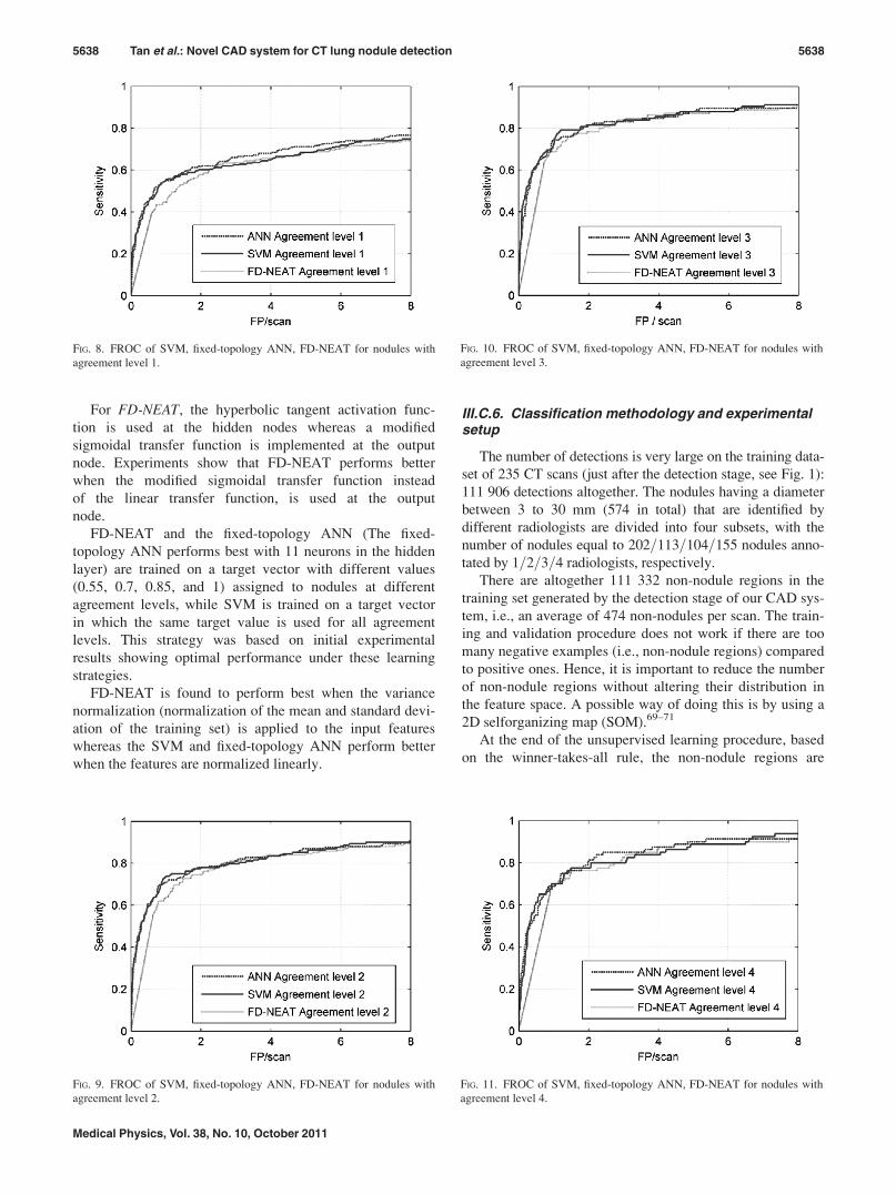
FIG. 8. FROC of SVM, fixed-topology ANN, FD-NEAT for nodules with

agreement level 1.


agreement level 2.


agreement level 3.


agreement level 4.



clustered into different cells of the Kohonen layer based on

the similarities between the properties represented in each

feature vector. Subsets of the examples extracted from each

cell should be representative of the original dataset. The

number of cells is automatically determined by a function in

the toolbox that returns a classification error measure defined

by the creators of the toolbox.71 A SOM of 53� 32 output

nodes is generated by the program in a hexagonal lattice.

The original set of non-nodule regions is reduced to 3382

examples by extracting 3%–6% or 1–2 examples from each

representative class, i.e., each output node of the SOM. The

final training set consists of the negative examples extracted

by the SOM in combination with the annotated lesions of

positive cases.

As in any GA procedure, several runs or repetitions have

to be performed to find the optimal FD-NEAT network over

the entire search space. This is standard practice in the field of

evolutionary intelligence.39,41,62 The networks are evolved in

a population of 200 networks over 200 generations. The best

network, i.e., the network with the highest fitness (computed

using a fitness function based on the classification accuracy

defined in Ref. 41 and used in Ref. 39) on the training set at

the end of the evolutionary process over ten runs is used to

classify the nodules in the test set. Additional details of the pa-

rameter values that are implemented in the FD-NEAT algo-

rithm are provided in Appendix B. We modified Christian

Mayr’s software, NEAT-Matlab (Ref. 72), to program the

FD-NEAT classifier required for our experiments.

IV. RESULTS

The independent test set consists of 125 CT scans. For the

nodules in the test set, the following distribution is applica-

ble: 87=46=46=80 TPs annotated by 1=2=3=4 out of 4 radiol-

ogists, respectively.

The detection stage yields 56 865 candidate detections al-

together. Of the nodule candidates, a total of 64=44=43=79

nodules are detected, which correspond to sensitivities of

88.8%=96.5%=96.8%=98.8% at agreement levels 1=2=3=4.

The average number of FPs per scan computed at their re-

spective agreement levels is 456.7=457.3=457.6=458.0 at

this point (after the detection stage) of the CAD system. The

system’s scoring method reports a detection as a TP if its

center of mass (or centroid) is within a specified Euclidean

distance of the center of mass of an annotation. For an anno-

tation with a volume less than 600 voxels (or mm3), the dis-

tance is set to 5 voxels (or 5 mm). For bigger nodules with

volumes exceeding 600 voxels, the distance threshold is set

to 9 voxels.

The scoring method is based on the distance between the

nodule candidate centroid as proposed by our system and the

centroid of the radiologist’s annotation, and the distance

threshold is derived from the radii of the annotations (see

Refs. 28 and 34). The range of the nodule sizes in the LIDC

database is 1.5 to 15 mm in radius, assuming the nodules are

spherical. At a volume of 600 mm3, the volume-equivalent-

radius r (assuming that the volume is spherical) via the for-

mula r ¼ffiffiffiffiffiffiffiffiffiffiffiffiffi3�volume

4p3

qis equal to 5.2 mm. Hence, for nodules

with a volume smaller than 600 mm3, we set the threshold

for reporting a TP detection to 5 mm (slightly stricter than

the obtained 5.2 mm for a volume equal to 600 mm3). From

the histogram of volumes in the database (i.e., the 360 cases

used), we see that radii less than 5 mm cover about 75% of

the annotated nodules. Relaxing the distance criterion

towards larger values might only slightly improve the TP

rate for nodules with volumes less than 600 mm3 at the risk

of introducing much more FPs. Similarly, nodules with radii

between 5 mm and 9 mm represent approximately 75% of

the remaining annotations. For those nodules, we adopt a

distance threshold of 9 mm. For nodules with radii larger

than 9 mm (maximum radius in the database is 15 mm) we

do not relax the previous distance threshold towards higher

values as this might only slightly improve the TP rate at the

TABLE III. CAD system sensitivities of FD-NEAT, the fixed-topology ANN and the SVM classifiers at an FP rate of 4=scan for nodules at the four agreement

levels.

Sensitivity

Agreement level FD-NEAT ANN SVM

1 170=259 * 100%¼ 65.6% 176=259 * 100%¼ 68.0% 168=259 * 100%¼ 64.9%

2 144=172 * 100%¼ 83.7% 143=172 * 100%¼ 83.1% 143=172 * 100%¼ 83.1%

3 109=126 * 100%¼ 86.5% 107=126 * 100%¼ 84.9% 108=126 * 100%¼ 85.7%

4 70=80 * 100%¼ 87.5% 70=80 * 100%¼ 87.5% 67=80 * 100%¼ 83.8%

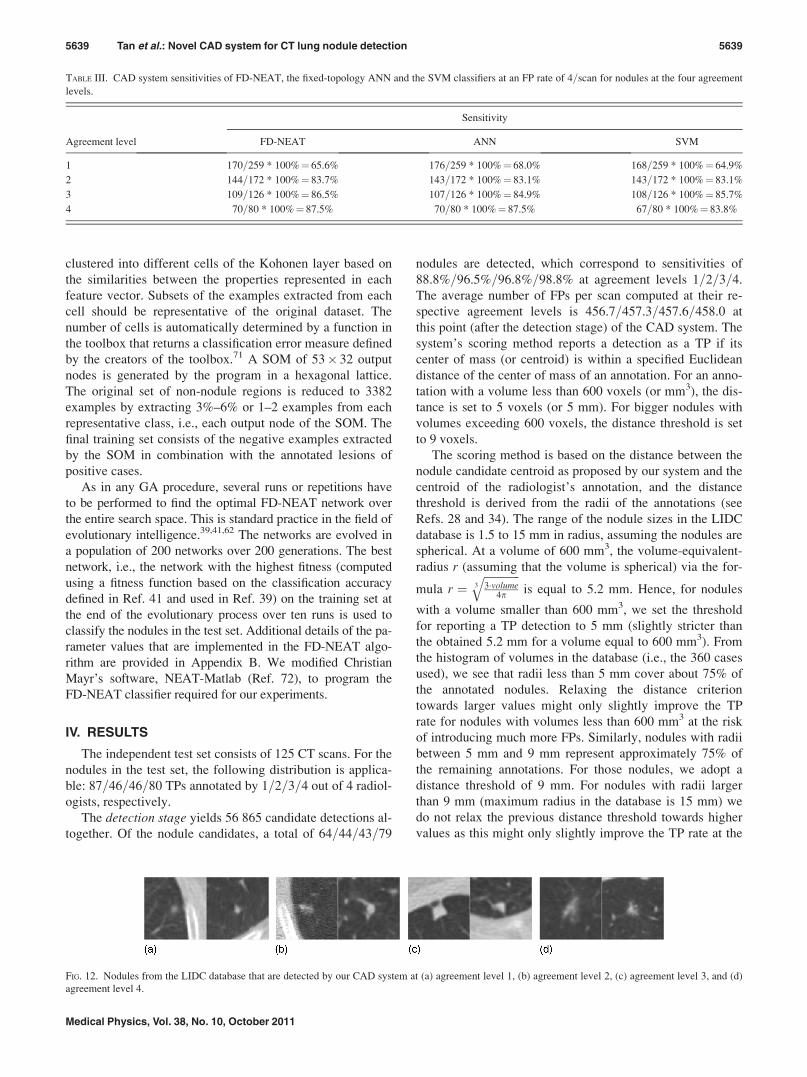
FIG. 12. Nodules from the LIDC database that are detected by our CAD system at (a) agreement level 1, (b) agreement level 2, (c) agreement level 3, and (d)

agreement level 4.



risk of introducing much more FPs. The thresholds 5 and 9

mm are therefore a reasonable compromise for defining the

scoring rules.

The features of the candidate nodules are normalized (see

Sec. III C 5) and fed to the inputs of the three different clas-

sifiers. Figure 5 shows the free-response receiver operating

characteristic (FROC) curves of the FD-NEAT classifier for

nodules with different agreement levels. Figure 6 displays

the same FROC curves for the fixed-topology ANN classifier

and Fig. 7 for the SVM classifier. It can be observed in all

the results that the sensitivities are generally higher for nod-

ules identified at higher consensus among the four radiolog-

ists with considerably better results at agreement levels 2–4

compared to agreement level 1. Figures 8–11 show the

FROC curves comparing the performances of the three clas-

sifiers at agreement levels 1–4, respectively. Table III dis-

plays the CAD system sensitivities at all agreement levels

for the FD-NEAT classifier, fixed-topology ANN, and SVM

classifiers, respectively, obtained at a FP rate of 4 per scan,

which is an acceptable FP rate used by other CAD systems

in the literature.5,26,31

From the detection results at different agreement levels

(Figs. 5–11), it can be observed that all three classifiers per-

form comparably well, with the fixed-topology ANN classi-

fier’s overall performance slightly exceeding that of SVM

and FD-NEAT. The results of the fixed-topology ANN clas-

sifier display a clear trend whereby the results are better at

higher agreement levels. The results of SVM and FD-NEAT

also display the same trend whereby better overall perform-

ance is generally obtained at higher agreement levels. It can

also be observed from Figs. 5–7 that for all three classifiers,

the CAD sensitivities at agreement levels 2–4 are consider-

ably higher than at agreement level 1. Slight increases in per-

formance can be observed when the number of agreement

levels is incremented from 2 to 4, but the improvements in

performance are much less obvious than the considerable

increase observed between agreement levels 1 and 2.

If we compare the performances of the three classifiers at

fixed agreement levels (Figs. 8–11), it can be observed that

the fixed-topology ANN generally outperforms the other two

classifiers at agreement levels 1–4. At agreement levels 2

and 3, FD-NEAT’s performance is the best between FP rates

of 3–4 per scan. Conversely, SVM’s performance exceeds

the other two classifiers between FP rates of 1–2 FP per scan

at agreement levels 2 and 3.

From Table III, it can be observed that at an FP rate of 4

FP=scan, FD-NEAT’s performance is highest at agreement

level 3: 109 out of 126 nodules that are annotated by at least

three radiologists are detected, which yields a sensitivity of

86.5%. The fixed-topology ANN performs best on nodules

with agreement level 1, achieving a sensitivity of 68.0%.

FD-NEAT and the fixed-topology ANN both achieve the

highest sensitivity of 87.5% on nodules with agreement level

4. FD-NEAT also performs best on nodules with agreement

level 2, namely, 144 out of 172 nodules annotated by at least

two radiologists are detected giving a sensitivity of 83.7% at

4 FP=scan. Examples, at different agreement levels, of

detected nodules are shown in Fig. 12. Examples of nodules

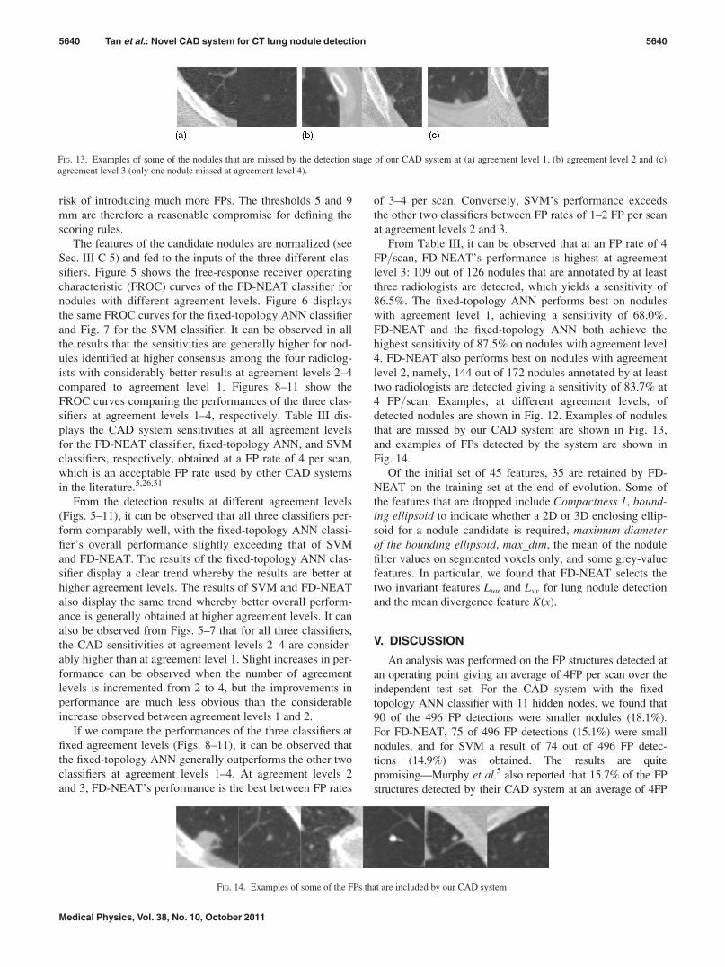
that are missed by our CAD system are shown in Fig. 13,

and examples of FPs detected by the system are shown in

Fig. 14.

Of the initial set of 45 features, 35 are retained by FD-

NEAT on the training set at the end of evolution. Some of

the features that are dropped include Compactness 1, bound-ing ellipsoid to indicate whether a 2D or 3D enclosing ellip-

soid for a nodule candidate is required, maximum diameterof the bounding ellipsoid, max_dim, the mean of the nodule

filter values on segmented voxels only, and some grey-value

features. In particular, we found that FD-NEAT selects the

two invariant features Luu and Lvv for lung nodule detection

and the mean divergence feature K(x).

V. DISCUSSION

An analysis was performed on the FP structures detected at

an operating point giving an average of 4FP per scan over the

independent test set. For the CAD system with the fixed-

topology ANN classifier with 11 hidden nodes, we found that

90 of the 496 FP detections were smaller nodules (18.1%).

For FD-NEAT, 75 of 496 FP detections (15.1%) were small

nodules, and for SVM a result of 74 out of 496 FP detec-

tions (14.9%) was obtained. The results are quite

promising––Murphy et al.5 also reported that 15.7% of the FP

structures detected by their CAD system at an average of 4FP

FIG. 13. Examples of some of the nodules that are missed by the detection stage of our CAD system at (a) agreement level 1, (b) agreement level 2 and (c)

agreement level 3 (only one nodule missed at agreement level 4).

FIG. 14. Examples of some of the FPs that are included by our CAD system.



per scan were smaller nodules. Some other FP structures

appear to be vessel junctions and branches, and a high

proportion of them are mediastinal and pleural structures.

Future research includes methods for eliminating FP structures,

such as improved differentiation between nodules and blood

vessels.

The slightly lower performance of FD-NEAT (see FROC

curves) with respect to SVM and the fixed-topology ANN is

unexpected, given the previously observed performance of

FD-NEAT on sample benchmarking examples.39,73 A plausi-

ble explanation is the complexity of the task at hand. In the

lung nodule detection task, starting with a minimal topology

might not be so optimal.

A rigorous comparison with other systems is difficult due

to variability in the image datasets used (e.g., number of

cases, scanning protocols, slice thickness, and spacing), the

implemented labeling and scoring methods, the differences

in applied validation and ground truth standards, and the dif-

ferences in nodule types and sizes in the image databases.

These differences have high impact on the performance of a

CAD system. Nevertheless, it is important to attempt making

a relative comparison––see Tables IV and V:

- Golosio et al.26 report the performance of a novel multi-

threshold method on 23 scans from the Italung-CT data-

base and 83 scans from the LIDC database. We compare

the performance of our method with theirs on LIDC for

nodules evaluated at agreement levels 2–4.

- In Ref. 74, Gori et al. propose a voxel-based neural

approach to detect lung nodules in the framework of the

MAGIC-5 Italian project. In Table IV, we report the results

of their method on 75 internal nodules belonging to 34

low-dose CT scans.

- Murphy et al.5 report on a large-scale evaluation of a

method using local image features and k-Nearest-Neighbor

classification in the framework of the Nelson Trial lung

cancer screening program. The results reported in Table IV

are obtained from an image database consisting of 813

scans annotated by two radiologists.

- Opfer and Wiemker31 present a validation study of a CAD

system on images from LIDC and discuss how the per-

formance of their algorithm is influenced by the choice of

underlying ground truth.

- Sahiner et al.30 report on the performance of a 3D region

growing method and a 3D active contour model on a test

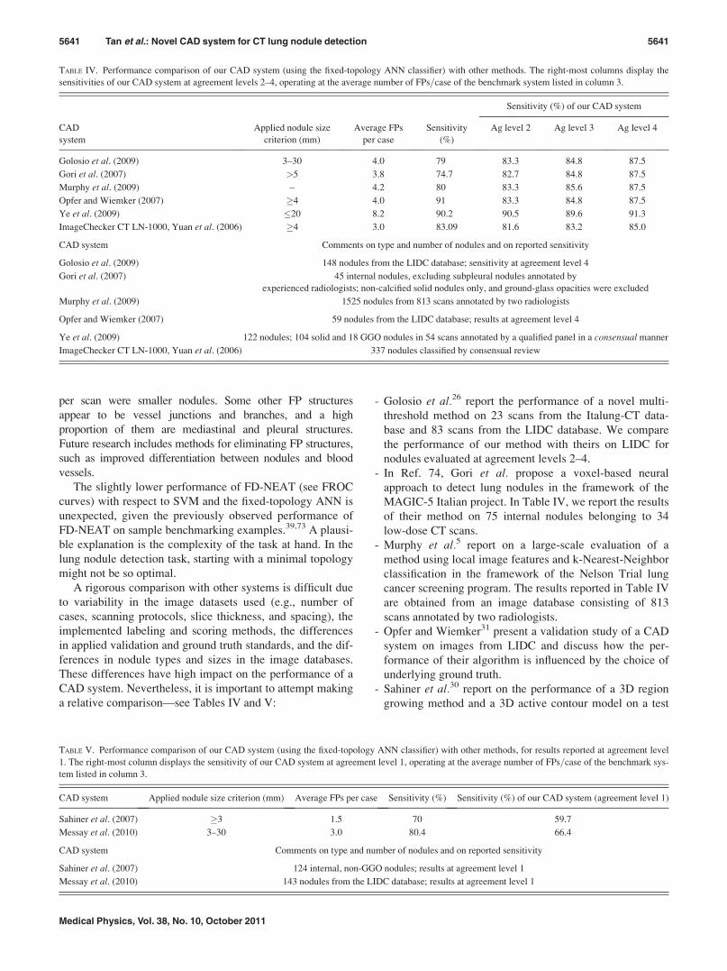
TABLE IV. Performance comparison of our CAD system (using the fixed-topology ANN classifier) with other methods. The right-most columns display the

sensitivities of our CAD system at agreement levels 2–4, operating at the average number of FPs=case of the benchmark system listed in column 3.

Sensitivity (%) of our CAD system

CAD

system

Applied nodule size

criterion (mm)

Average FPs

per case

Sensitivity

(%)

Ag level 2 Ag level 3 Ag level 4

Golosio et al. (2009) 3–30 4.0 79 83.3 84.8 87.5

Gori et al. (2007) >5 3.8 74.7 82.7 84.8 87.5

Murphy et al. (2009) – 4.2 80 83.3 85.6 87.5

Opfer and Wiemker (2007) �4 4.0 91 83.3 84.8 87.5

Ye et al. (2009) �20 8.2 90.2 90.5 89.6 91.3

ImageChecker CT LN-1000, Yuan et al. (2006) �4 3.0 83.09 81.6 83.2 85.0

CAD system Comments on type and number of nodules and on reported sensitivity

Golosio et al. (2009) 148 nodules from the LIDC database; sensitivity at agreement level 4

Gori et al. (2007) 45 internal nodules, excluding subpleural nodules annotated by

experienced radiologists; non-calcified solid nodules only, and ground-glass opacities were excluded

Murphy et al. (2009) 1525 nodules from 813 scans annotated by two radiologists

Opfer and Wiemker (2007) 59 nodules from the LIDC database; results at agreement level 4

Ye et al. (2009) 122 nodules; 104 solid and 18 GGO nodules in 54 scans annotated by a qualified panel in a consensual manner

ImageChecker CT LN-1000, Yuan et al. (2006) 337 nodules classified by consensual review

TABLE V. Performance comparison of our CAD system (using the fixed-topology ANN classifier) with other methods, for results reported at agreement level

1. The right-most column displays the sensitivity of our CAD system at agreement level 1, operating at the average number of FPs=case of the benchmark sys-

tem listed in column 3.

CAD system Applied nodule size criterion (mm) Average FPs per case Sensitivity (%) Sensitivity (%) of our CAD system (agreement level 1)

Sahiner et al. (2007) �3 1.5 70 59.7

Messay et al. (2010) 3–30 3.0 80.4 66.4

CAD system Comments on type and number of nodules and on reported sensitivity

Sahiner et al. (2007) 124 internal, non-GGO nodules; results at agreement level 1

Messay et al. (2010) 143 nodules from the LIDC database; results at agreement level 1



set of 33 scans from patient files at the University of Mich-

igan and 29 scans from the LIDC database. The sensitivity

result of the combined methods at 1.5 FP=scan is given in

Table V.

- In a recent paper, Messay et al.32 present and analyze a

CAD system based on thresholding and a morphological

opening operation, many 3D nodule candidate features,

and linear and quadratic discriminant classifiers. Valida-

tion on 143 nodules at agreement level 1 from 84 CT scans

of LIDC yields a sensitivity of 80.4% at 3 FP=scan.

- A shape-based method using a volumetric shape index map,

a “dot” map, antigeometric diffusion, and modified

expectation-maximization methods for nodule segmentation

is proposed by Ye et al.17 It is applied on a dataset consist-

ing of 108 thoracic CT scans using a wide range of x-ray

tube currents. The dataset is split into a training and inde-

pendent test set, and a sensitivity of 90.2%, at a FP rate of

8.2 FP=scan, is reported.

- The results of a commercially available CAD system, i.e., the

ImageChecker CT LN-1000 system by R2 Technology is an-

alyzed by Yuan et al.75 on a dataset of 150 patients. The orig-

inal 1.25 mm axial slice images are used for the CAD

system; the images are reconstructed with 2.5 mm slice thick-

ness for radiologist evaluation. There are altogether 337 nod-

ules that are equal to or exceed 4 mm in diameter in the test

dataset on consensual review. The sensitivity of the Image-

Checker on the nodules is 83.09% at 3 FP=scan.

From Table IV, it can be observed that the performance

of our method compares very well with that of other methods

in terms of sensitivity of detection at the given FP rates.

With the exception of the work of Opfer and Wiemker,31 the

sensitivities obtained by our CAD system are generally

higher than other methods. However, the reader is reminded

that Opfer and Wiemker present their results on nodules of 4

mm diameter and above, whereas our method is validated on

the original nodule outlines of the LIDC database on nodules

of diameter 3 mm and above. Table V compares the per-

formance of our method with other methods who report their

results at agreement level 1. In the LIDC database, this

means that nodules which are annotated by only one out of

four radiologists after the unblinded review are also included

in the definition of the gold standard with respect to which

the CAD system’s performance is evaluated. Comparatively,

the sensitivity results of our CAD system are much lower at

agreement level 1 (refer to Table V). Much higher sensitiv-

ities are obtained on our system at agreement levels 2 and

above (see Table IV). However, correct results at agreement

level 1 might not be truly indicative of the good performance

of a CAD system since the majority of the radiologists did

not indicate them as lung nodules.

VI. CONCLUSIONS

We have presented a complete CAD system for lung nod-

ule detection. For the initial detection stage, we have intro-

duced a novel method for finding seed points based on the

maxima of the divergence of the normalized image gradient

(DNG), and we have exploited previously published nodule

and vessel enhancement filters. The subsequent classificationstage input consists of invariant features calculated in 3D

gauge coordinates, the DNG feature and other geometric and

grey-value descriptors. A novel feature-selective classifier

based on ANNs and genetic algorithms (FD-NEAT) was

introduced for the first time in such a complex problem as

lung nodule detection and compared to two other more estab-

lished and commonly used classifiers, namely the SVM classi-

fier and a fixed-topology ANN. Although FD-NEAT remains

attractive due to its flexibility and adaptability without having

to make a priori and inevitably heuristic choices on the ANN

topology and complexity, its overall performance is slightly

outperformed by the fixed-topology ANN classifier. The best

fixed-topology ANN classifier (with 11 internal nodes)

achieves a sensitivity of 87.5% at a rate of 4 FP=scan on nod-

ules with a diameter greater than or equal to 3 mm, on an in-

dependent test set of 125 cases of the LIDC database with the

subset of nodules that were annotated by four radiologists.

Comparisons with other methods illustrate that our CAD

system––with all three considered classifiers––is performing

well compared to other methods in the literature.

APPENDIX A: LIDC CASES USED FOR TRAINING ANDTESTING

All the scans in the LIDC database are preceded by the num-

bers “13614193285030,” followed by another three numbers for

identification and experimental repeatability. Of the entire data-

base of 399 cases, two were missing. The cases that were used

in the independent test set (125 cases altogether) are: 22, 24, 30,

32, 35, 42, 46, 48, 53, 58, 61, 66, 75, 88, 89, 95, 101, 102, 112,

113, 126, 140, 146, 150, 152, 154, 159, 163, 168, 170, 172, 174,

178, 180, 184, 187, 190–192, 195, 197, 201, 205, 207, 208, 210,

212, 216, 218, 220, 221, 223, 225, 230, 233, 236, 239, 241, 250,

254, 256, 258, 260, 261, 266, 271, 276, 279, 290–292, 297, 299,

303, 305, 309, 311, 314, 315, 317, 320, 323, 324, 326, 329,

333–335, 338, 341, 342, 344, 347, 350, 351, 353, 357, 358, 361,

370, 373, 377, 378, 381, 387, 389, 399, 401, 404, 410, 416, 418,

422, 423, 427, 428, 431, 434, 439, 444, 450, 505, 507, 508, and

511. The other scans in the database were used for training the

classifiers (235 cases altogether) with the exception of scans

633, 642, 644, 646, 647, 648, 649, 650, 653, and 654, which did

not have radiologists’ annotations, scan 537, which had missing

intermittent slices, and scan 459 in which the annotations did not

correspond to the image. We also excluded the contrast-

enhanced images acquired with the Toshiba scanner (25 cases

altogether) for training or testing purposes due to image format-

ting problems.

APPENDIX B: FD-NEAT SYSTEM PARAMETERS––TECHNICAL DESCRIPTION

Notations and terminology are referring to Refs. 39, 41, and

76. Each population has 200 networks. The coefficients for

measuring compatibility are c1 (coefficient to determine the im-

portance of excess genes in measuring compatibility)¼ 1.0, c2

(coefficient to determine the importance of disjoint genes in



measuring compatibility)¼ 1.0, and c3 (coefficient to determine

the importance of average weight difference in measuring

compatibility)¼ 0.3. The initial compatibility distance for spe-

ciation, Ct is 8.0. However, because the population dynamics

can be unpredictable over the course of evolution, we assign a

target of 10 species. If the number of species exceeds 10, Ct is

increased by 4.0 to reduce the number of species. Conversely,

if the number of species is less than 10, Ct is decreased by 4.0

to increase the number of species. Parameters to measure stag-

nation in species fitness are disabled so that species cannot die

out. When the maximum overall fitness of the population does

not change within a specified refocus threshold of 0.01 for 20

generations, only the top two species are allowed to reproduce.

The percentage of each species that is eliminated from the low-

est performing individuals is 80%. The champion of each spe-

cies with more than five networks is copied unchanged into the

next generation. There is a 20% probability of a connection

gene having its weight mutated. There is a 10% chance that an

inherited gene is re-enabled in the offspring if it is inherited dis-

abled. Conversely, there is a 15% chance that an inherited gene

is disabled in the offspring if it is inherited enabled. This proba-

bility only applies to the initial input connections and is the

principle of selecting relevant features for FD-NEAT. The

probability that recurrent connections are formed is put to zero.

There is a 20% chance of crossover in the entire population. In

40% of crossovers, the offspring inherits the average of the

connection weights of matching genes from both parents,

instead of the connection weight of a randomly selected parent.

The interspecies mating rate, i.e., the probability that the

parents in the standard crossover process originate from differ-

ent species is only 5%. The probability of adding a new node is

set initially to 0.5 and the probability of adding a new link or

connection to 0.8. After 20 generations from the start of evo-

lution, the add node probability is changed to 0.05 and the

add link probability to 0.9. After 45 generations, the add link

probability is modified to be 0.1, whereas the add node proba-

bility is maintained at 0.05. These parameter values are found

experimentally and follow a logical pattern, namely, links

need to be added considerably more often than nodes. At the

start of evolution, higher add node and add link probabilities

should be assigned to FD-NEAT as it starts with almost mini-

mal topology. Eventually, when FD-NEAT has gained signifi-

cant structure, the probabilities of adding new structure can be

reduced.

ACKNOWLEDGMENTS

The authors would like to thank Yung Yi Chew for his

work on the MatlabVR differential invariance toolbox in 2D

and 3D. This work is also supported by the IAP project from

the federal agency Belspo P6=38 NIMI.

1G. Coppini, S. Diciotti, M. Falchini, N. Villari and G. Valli, “Neural net-

works for computer-aided diagnosis: Detection of lung nodules in chest

radiograms,” IEEE Trans. Inf. Technol. Biomed. 7, 344–357 (2003).2A. M. R. Schilham, B. van Ginneken, and M. Loog, “A computer-aided di-

agnosis system for detection of lung nodules in chest radiographs with an

evaluation on a public database,” Med. Image Anal. 10, 247–258 (2006).

3A. H. Baydush, D. M. Catarious, J. Y. Lo, C. K. Abbey, and C. E. Floyd,

“Computerized classification of suspicious regions in chest radiographs

using subregion Hotelling observers,” Med. Phys. 28, 2403–2409 (2001).4H. Arimura, S. Katsuragawa, K. Suzuki, F. Li, J. Shiraishi, S. Sone, and K.

Doi, “Computerized scheme for automated detection of lung nodules in

low-dose computed tomography images for lung cancer screening,” Acad.

Radiol. 11, 617–629 (2004).5K. Murphy, B. vanGinneken, A. M. R. Schilham, B. J. deHoop, H. A. Gie-

tema, and M. Prokop, “A large-scale evaluation of automatic pulmonary

nodule detection in chest CT using local image features and k-nearest-

neighbour classification,” Med. Image Anal. 13, 757–770 (2009).6S. V. Fotin, A. P. Reeves, A. M. Biancardi, D. F. Yankelevitz, and C. I.

Henschke, “A multiscale Laplacian of Gaussian filtering approach to auto-

mated pulmonary nodule detection from whole-lung low-dose CT scans,”

Proc. SPIE 7260, 72601Q (2009).7I. C. Sluimer, P. F. vanWaes, M. A. Viergever, and B. vanGinneken,

“Computer-aided diagnosis in high resolution CT of the lungs,” Med.

Phys. 30, 3081–3090 (2003).8R. Wiemker, P. Rogalla, A. Zwartkruis, and T. Blaffert, “Computer aided

lung nodule detection on high resolution CT data,” Proc. SPIE 4684,

677–688 (2002).9S. Iwano, T. Nakamura, Y. Kamioka, M. Ikeda, and T. Ishigaki, “Computer-

aided differentiation of malignant from benign solitary pulmonary nodules

imaged by high-resolution CT,” Comput. Med. Imaging Graph. 32, 416–422

(2008).10S. G. Armato, G. McLennan, M. F. McNitt-Gray, C. R. Meyer, D. Yankele-

vitz, D. R. Aberle, C. I. Henschke, E. A. Hoffman, E. A. Kazerooni, H.

MacMahon, A. P. Reeves, B. Y. Croft, L. P. Clarke, and C. Lung Image

Database, “Lung image database consortium: Developing a resource for the

medical imaging research community,” Radiology 232, 739–748 (2004).11ELCAP Lab, “ELCAP Public Lung Image Database, (http://www.via.cor-

nell.edu/databases/lungdb.html, Last accessed: October 2010, 2003).12M. Dolejsi, J. Kybic, M. Polovincak, and S. Tuma, “The lung time-

annotated lung nodule dataset and nodule detection framework,” Proc.

SPIE 7260, 72601U (2009).13B. v. Ginneken, S. G. Armato, B. d. Hoop, S. v. A.-v. d. Vorst, T. Duin-

dam, M. Niemeijer, K. Murphy, A. Schilham, A. Retico, M. E. Fantacci,

N. Camarlinghi, F. Bagagli, I. Gori, T. Hara, H. Fujita, G. Gargano, R.

Bellotti, S. Tangaro, L. Bolanos, F. D. Carlo, P. Cerello, S. C. Cheran, E.

L. Torres, and M. Prokop, “Comparing and combining algorithms for

computer-aided detection of pulmonary nodules in computed tomography

scans: The ANODE09 study,” Med. Image Anal. 14, 707–722 (2010).14American Cancer Society, “Cancer Facts and Figures,” (2009).15S. G. Armato, M. B. Altman, and P. J. LaRiviere, “Automated detection of

lung nodules in CT scans: Effect of image reconstruction algorithm,”

Med. Phys. 30, 461–472 (2003).16D. S. Paik, C. F. Beaulieu, G. D. Rubin, B. Acar, R. B. Jeffrey, J. Yee, J.

Dey, and S. Napel, “Surface normal overlap: A computer-aided detection

algorithm, with application to colonic polyps and lung nodules in helical

CT,” IEEE Trans. Med. Imaging 23, 661–675 (2004).17X. J. Ye, X. Y. Lin, J. Dehmeshki, G. Slabaugh, and G. Beddoe, “Shape-

based computer-aided detection of lung nodules in thoracic CT images,”

IEEE Trans. Biomed. Eng. 56, 1810–1820 (2009).18Y. Lee, T. Hara, H. Fujita, S. Itoh, and T. Ishigaki, “Automated detection of

pulmonary nodules in helical CT images based on an improved template-

matching technique,” IEEE Trans. Med. Imaging 20, 595–604 (2001).19L. Boroczky, L. Zhao, and K. P. Lee, “Feature subset selection for improv-

ing the performance of false positive reduction in lung nodule CAD,”

IEEE Trans. Inf. Technol. Biomed. 10, 504–511 (2006).20K. Suzuki and K. Doi, “How can a massive training artificial neural net-

work (MTANN) be trained with a small number of cases in the distinction

between nodules and vessels in thoracic CT?” Acad. Radiol. 12,

1333–1341 (2005).21K. Suzuki, Z. H. Shi, and J. Zhang, “Supervised enhancement of lung nod-

ules by use of a massive-training artificial neural network (MTANN) in

computer-aided diagnosis (CAD),” Proc. ICPR, 680–683 (2008).22K. Suzuki and K. Doi, “Characteristics of a massive training artificial neu-

ral network in the distinction between lung nodules and vessels in CT

images,” Proc. CARS 1268, 923–928 (2004).23K. Suzuki, F. Li, S. Sone, and K. Doi, “Computer-aided diagnostic scheme

for distinction between benign and malignant nodules in thoracic low-dose

CT by use of massive training artificial neural network,” IEEE Trans.

Med. Imaging 24, 1138–1150 (2005).



24M. S. Brown, M. F. McNitt-Gray, J. G. Goldin, R. D. Suh, J. W. Sayre, and

D. R. Aberle, “Patient-specific models for lung nodule detection and surveil-

lance in CT images,” IEEE Trans. Med. Imaging 20, 1242–1250 (2001).25Y. Kawata, N. Niki, H. Ohmatsu, and N. Moriyama, “Example-based

assisting approach for pulmonary nodule classification in three-

dimensional thoracic computed tomography images,” Acad. Radiol. 10,

1402–1415 (2003).26B. Golosio, G. L. Masala, A. Piccioli, P. Oliva, M. Carpinelli, R. Cataldo,

P. Cerello, F. DeCarlo, F. Falaschi, M. E. Fantacci, G. Gargano, P. Kasae,

and M. Torsello, “A novel multithreshold method for nodule detection in

lung CT,” Med. Phys. 36, 3607–3618 (2009).27J. J. Suarez-Cuenca, P. G. Tahoces, M. Souto, M. J. Lado, M. Remy-

Jardin, J. Remy, and J. J. Vidal, “Application of the iris filter for automatic

detection of pulmonary nodules on computed tomography images,” Com-

put. Biol. Med. 39, 921–933 (2009).28A. Retico, M. E. Fantacci, I. Gori, P. Kasae, B. Golosio, A. Piccioli, P.

Cerello, G. DeNunzio, and S. Tangaro, “Pleural nodule identification in

low-dose and thin-slice lung computed tomography,” Comput. Biol. Med.

39, 1137–1144 (2009).29Q. Li, F. Li, and K. Doi, “Computerized detection of lung nodules in thin-

section CT images by use of selective enhancement filters and an auto-

mated rule-based classifier,” Acad. Radiol. 15, 165–175 (2008).30B. Sahiner, L. M. Hadjilski, H. P. Chan, J. Z. Shi, T. Way, P. N. Cascade,

E. A. Kazerooni, C. Zhou, and J. Wei, “The effect of nodule segmentation

on the accuracy of computerized lung nodule detection on CT scans: Com-

parison on a data set annotated by multiple radiologists,” Proc. SPIE 6514,

65140L (2007).31R. Opfer and R. Wiemker, “Performance analysis for computer aided lung

nodule detection on LIDC data,” Proc. SPIE 6515, 65151C (2007).32T. Messay, R. C. Hardie, and S. K. Rogers, “A new computationally effi-

cient CAD system for pulmonary nodule detection in CT imagery,” Med.

Image Anal. 14, 390–406 (2010).33Z. Y. Ge, B. Sahiner, H. P. Chan, L. M. Hadjiiski, P. N. Cascade, N.

Bogot, E. A. Kazerooni, J. Wei, and C. A. Zhou, “Computer-aided detec-

tion of lung nodules: False positive reduction using a 3D gradient field

method and 3D ellipsoid fitting,” Med. Phys. 32, 2443–2454 (2005).34J. T. Pu, B. Zheng, J. K. Leader, X. H. Wang, and D. Gur, “An automated

CT based lung nodule detection scheme using geometric analysis of

signed distance field,” Med. Phys. 35, 3453–3461 (2008).35X. Zhang, J. Stockel, M. Wolf, P. Cathier, G. McLennan, E. A. Hoffman, and

M. Sonka, “A new method for spherical object detection and its application to

computer aided detection of pulmonary nodules in CT images,” in Proceed-ings of MICCAI, Springer Berlin=Heidelberg, 2007, Vol. 4791, pp. 842–849.

36Q. Li, “Recent progress in computer-aided diagnosis of lung nodules on

thin-section CT,” Comput. Med. Imaging Graph. 31, 248–257 (2007).37I. Sluimer, A. Schilham, M. Prokop, and B. vanGinneken, “Computer

analysis of computed tomography scans of the lung: A survey,” IEEE

Trans. Med. Imaging 25, 385–405 (2006).38L. Saba, G. Caddeo, and G. Mallarini, “Computer-aided detection of pul-

monary nodules in computed tomography: Analysis and review of the lit-

erature,” J. Comput. Assist. Tomogr. 31, 611–619 (2007).39M. Tan, M. Hartley, M. Bister, and R. Deklerck, “Automated Feature

Selection in Neuroevolution,” Evol. Intell. 4, 271–292 (2009).40M. E. Timin, “The robot auto racing simulator,” Available at http://rars.-

sourceforge.net (1995).41K. O. Stanley and R. Miikkulainen, “Evolving neural networks through

augmenting topologies,” Evol. Comput. 10, 99–127 (2002).42A. H. Salden, B. M. T. Romeny, M. A. Viergever, L. Florack, and J. J.

Koenderink, “Differential geometric description of 3D scalar images,”

Technical Report, 3D Computer Vision (Utrecht University Hospital, The

Netherlands, 1992).43B. M. t. H. Romeny, Front-End Vision & Multi-Scale Image Analysis.

(Springer Verlag, Berlin, 2003).44S. G. Armato, M. F. McNitt-Gray, A. P. Reeves, C. R. Meyer, G.

McLennan, D. R. Aberle, E. A. Kazerooni, H. MacMahon, E. J. R. van-

Beek, D. Yankelevitz, E. A. Hoffman, C. I. Henschke, R. Y. Roberts, M.

S. Brown, R. M. Engelmann, R. C. Pais, C. W. Piker, D. Qing, M. Kocher-

ginsky, B. Y. Croft, and L. P. Clarke, “The Lung Image Database Consor-

tium (LIDC): An evaluation of radiologist variability in the identification

of lung nodules on CT scans,” Acad. Radiol. 14, 1409–1421 (2007).45S. G. Armato, R. Y. Roberts, M. F. McNitt-Gray, C. R. Meyer, A. P. Reeves,

G. McLennan, R. M. Engelmann, P. H. Bland, D. R. Aberle, E. A. Kazer-

ooni, H. MacMahon, E. J. R. vanBeek, D. Yankelevitz, B. Y. Croft, and L. P.

Clarke, “The lung image database consortium (LIDC): Ensuring the integrity

of expert-defined ‘truth’,” Acad. Radiol. 14, 1455–1463 (2007).46W. D. Turner, T. P. Kelliher, J. C. Ross, and J. V. Miller, “An analysis of

early studies released by the Lung Imaging Database Consortium

(LIDC),” in Proceedings of MICCAI, Springer Berlin=Heidelberg, 2006,

Vol. 4191, pp. 487–494.47M. Dolejsi, and J. Kybic, “Automatic two-step detection of pulmonary

nodules,” Proc. SPIE 6514, 65143J (2007).48Q. Li, S. Sone, and K. Doi, “Selective enhancement filters for nodules,

vessels, and airway walls in two- and three-dimensional CT scans,” Med.

Phys. 30, 2040–2051 (2003).49Q. Li, H. Arimura, and K. Doi, “Selective enhancement filters for lung

nodules, intracranial aneurysms, and breast microcalcifications,” Proc.

CARS 1268, 929–934 (2004).50G. Agam, S. G. Armato, and C. H. Wu, “Vessel tree reconstruction in tho-

racic CT scans with application to nodule detection,” IEEE Trans. Med.

Imaging 24, 486–499 (2005).51A. P. Reeves, A. B. Chan, D. F. Yankelevitz, C. I. Henschke, B. Kressler,

and W. J. Kostis, “On measuring the change in size of pulmonary nod-

ules,” IEEE Trans. Med. Imaging 25, 435–450 (2006).52S. Diciotti, S. Lombardo, G. Coppini, L. Grassi, M. Falchini, and M. Mas-

calchi, “The LoG characteristic scale: a consistent measurement of lung

nodule size in CT imaging,” IEEE Trans. Med. Imaging 29, 397–409

(2010).53A. Retico, P. Delogu, M. E. Fantacci, I. Gori, and A. P. Martinez, “Lung

nodule detection in low-dose and thin-slice computed tomography,” Com-

put. Biol. Med. 38, 525–534 (2008).54L. M. J. Florack, B. M. T. Romeny, J. J. Koenderink, and M. A. Viergever,

“General intensity transformations and 2nd-order invariants,” Theory

Appl. Image Anal. 2, 22–29 (1992).55J. B. A. Maintz, P. A. van den Elsen, and M. A. Viergever, “Evaluation of

ridge seeking operators for multimodality medical image matching,” IEEE

Trans. Pattern Anal. Mach. Intell. 18, 353–365 (1996).56J. B. Maintz, P. A. van den Elsen, and M. A. Viergever, “Comparison of

feature-based matching of CT and MR brain images,” Proc. CVR Med’95

(Springer Verlag, 1995), Vol. 905, pp. 219–228.57T. Tuytelaars and K. Mikolajczyk, “Local invariant feature detectors: A

survey,” Found. Trends Comput. Graph. Vision 3, 177–280 (2007).58Y. Y. Chew, “2D and 3D Differential Invariance for Advanced Signal

Processing,” Master’s thesis, School of Electrical and Electronics Engi-

neering, Faculty of Engineering, University of Nottingham Malaysia Cam-

pus, Semenyih (2007).59M. Tan, M. Bister, and R. Deklerck, “Experiments on new combinations

of gauge derivatives in both 2D and 3D test images,” Technical Report

(Department of Electronics and Informatics (ETRO), Vrije Universiteit

Brussel, Belgium, 2010).60L. G. Kachiyan, “Rounding of polytopes in the real number model of

computation,” Math. Oper. Res. 21, 307–320 (1996).61N. Moshtagh, “Minimum volume enclosing ellipsoids,” Technical Report

(University of Pennsylvania, Pennsylvania, 2009).62S. Whiteson, P. Stone, K. O. Stanley, R. Mikkulainen, and N. Kohl,

“Automatic feature selection in neuroevolution,” in Proceedings of Geneticand Evolutionary Computation Conference (GECCO) (ACM New York,

Washington D.C., 2005), pp. 1225–1232.63S. Whiteson, K. O. Stanley, and R. Mikkulainen, “Automatic feature

selection in neuroevolution,” in Proceedings of Genetic and EvolutionaryComputation Conference (GECCO-2004) Workshop Program (New York,

NY: Springer-Verlag, 2004).64A. Ethembabaoglu and S. Whiteson, “Automatic feature selection using

FS-NEAT,” Technical report IAS-UVA-08-02 (Intelligent Autonomous

Systems Group, University of Amsterdam, The Netherlands, 2008).65C.-C. Chang and C.-J. Lin, “LIBSVM- A library for support vector machines,”

http://www.csie.ntu.edu.tw/~cjlin/libsvm/, Last accessed: July 2010.66C.-W. Hsu, C.-C. Chang, and C.-J. Lin, “A practical guide to support vec-

tor classification,” Technical Report (National Taiwan University, Taipei

106, Taiwan, 2009).67D. Marquardt, “An algorithm for least-squares estimation of nonlinear

parameters,” SIAM J. Appl. Math. 11, 431–441 (1963).68M. T. Hagan and M. Menhaj, “Training feed-forward networks with the

Marquardt algorithm,” IEEE Trans. Neural Networks 5, 989–993 (1999).69T. Kohonen, Self-Organizing Maps, 2nd ed. (Springer, Heidelberg, 1997).70T. Kohonen, Self-Organization and Associative Memory, 3rd ed.

(Springer-Verlag, Berlin, Heidelberg, 1988).



71J. Vesanto, J. Himberg, E. Alhoniemi, and J. Parhankangas, “Self-organiz-

ing map in Matlab: The SOM toolbox,” Laboratory of Information and

Computer Science, Helsinki University of Technology (http://www.cis.

hut.fi/projects/somtoolbox/about; Last accessed: October 2010).72C. Mayr, “NEAT Matlab,” (http://nn.cs.utexas.edu/?neatmatlab, 2003).73B. Jansen, M. Tan, I. Bautmans, B. V. Keymolen, T. Mets, and R. Deklerck,

“Accelerometer based gait analysis––Multi variate assessment of fall risk

with FD-NEAT,” in Proceedings of Biosignals (Rome, Italy, 2011).

74I. Gori, M. E. Fantacci, A. Preite Martinez, and A. Retico, “An automated

system for lung nodule detection in low-dose computed tomography,”

Proc. SPIE 6514, 65143R (2007).75R. Yuan, P. M. Vos, and P. L. Cooperberg, “Computer-aided detection in

screening CT for pulmonary nodules,” Am. J. Roentgenol. 186,

1280–1287 (2006).76K. O. Stanley, “Efficient evolution of neural networks through complex-

ification,” Ph.D. thesis (The University of Texas at Austin, Austin, 2004).



Documents

A novel computer-aided lung nodule detection system for … · A novel computer-aided lung nodule detection system for CT images Maxine Tan Department of Electronics and Informatics