1

A Theil decomposition of Latin American income distribution in the 20thCentury: Inverting the Kuznets Curve?

E.H.P.Frankema

Groningen Growth and Development CentreUniversity of Groningen

June 2006

AbstractThis paper applies a Theil decomposition method to investigate long run changes in the functionalincome distribution of 20th century Latin America. Kuznets argued that the economic transitionfrom a traditional rural into a modern urban economy eventually results, after an upswing in theearly phase of industrialisation, in sustained lower levels of personal income inequality (Kuznets’inverted U-curve hypothesis). In spite of various phases of strong economic growth and profoundstructural change a sustained decline in inequality has not taken place in Latin America. Thispaper argues that the apparent persistency of its inequality levels is the consequence of a trade-offbetween declining rural-urban income differences and increasing urban sector income differences.Urban sector inequality in a sample of major Latin American economies (Argentina, Brazil,Chile) was, from the start of the 20th century until the 1970’s, comparable to other advanced NewWorld economies (USA, Canada, Australia). Yet, since the 1970’s initial levels of rural and rural-urban inequality were overtaken by a rapid increase of urban inequality in virtually all LatinAmerican countries. In some cases this increase has been so pronounced that the Kuznets’ curveshould be “re-inverted” to accurately picture the secular inequality trend.

JEL Classification Numbers: N36, N60, O10, O15

Keywords: Latin America, Income Distribution, Kuznets Curve, Theil index, 20th Century

The author wishes to thank Jan Pieter Smits, Bart van Ark and Marcel Timmer for theiruseful comments on previous drafts.

Correspondence: Ewout Frankema, Groningen Growth and Development Centre,www.ggdc.net, Faculty of Economics, University of Groningen, P.O.Box 800, 9700 AV,Groningen, The Netherlands, e-mail: e.h.p.frankema@rug.nl, tel. +31-50-3637190, fax+31-50-363 7337

2

1 Introduction

The absence of a comprehensive conceptual framework in which all components of functionalincome1 are integrated is considered as an important shortcoming in distributional research(Atkinson 1997). Although literature pays attention to the “ultimate causes” of inequality such ascountries’ colonial antecedents, endowment structures, institutional systems and the impact ofglobalization,2 the empirical backbone remains largely confined to the partial assessment of wageand skill-differentials, neglecting the role of factor and sector income differentials: In studieswhere inequality is represented by a single “catch-all” gini-coefficient, functional incomecomponents remain hidden in the black-box all-together (Barro 2000, Forbes 2000). Bourguignonand Morrison argue that the role of economic dualism, and particularly of rural-urban dualism,appears to be largely ignored in recent literature (1998; p. 234).

Rural-urban dualism forms the cornerstone of Kuznets’ inequality theory. The basic ideais that changes in the functional income distribution as a result of urbanization andindustrialization (i.e. modern economic growth),3 change the structure of the personal incomedistribution (Williamson 1991). The theory has some appealing aspects. It incorporates the role ofasset distribution. It separates the effects of long run structural change from temporary economicshocks and disequilibria, such as hyperinflation, a debt crises or business cycle effects, on thepersonal distribution of income. And a practical advantage is the availability of an appropriateinstrument, the Theil index, which can be used to decompose the functional income distributionand study the complex of “proximate sources” of inequality in depth.

Studying long run changes in the personal income distribution in advanced industrialcountries Simon Kuznets concluded that the transition of a traditional rural into a modern urbaneconomy eventually results, after an upswing in the early phase of industrialisation, in sustainedlower levels of income inequality. In spite of various phases of rapid economic growth and

1 Functional income refers to income which can be directly related to its economic (functional) source,which can either be a production factor (labour, land, capital etc.) or a particular production sector activity.2 Engermann and Sokoloff 2000, Demsetz 1998, Acemoglu et.al. 2001, Acemoglu 2003, Frankema 2005,Wood 1994, Leamer 2000, Richardson 1995, Levy and Murnane 1992, Krugman 1995, Galor and Zeira1993, Gylfason and Zoega 1998, Goldin and Katz 1998, Easterly and Levine 2003, Leamer et.al. 1999,Spilimbergo et.al. 1999 , Persson and Tabellini 1992, Alesina and Rodrik 1994, De Soto 2000 etc..3 In his seminal paper Economic Growth and Income Inequality Simon Kuznets presented his ideasregarding “the character and causes of long term changes in the personal distribution of income” (1955:p.1). During the transition from a pre-modern rural economy to an advanced industrial economy personalincome inequality increases in the early stage and decreases in a later stage as economic growth sustainsand the industrial economy matures. In his book Modern Economic Growth. Rate, structure and spread,Kuznets distinghuishes modern economic growth from pre-modern economic growth as the era starting inGreat Britain in the second half of the eighteenth century, characterised by unprecedented and sustainedincreases in output per capita (or individual), or per worker, most often accompanied by an increase inpopulation and usually by great structural changes, that is, changes in social and economic institutions, orpractices. In modern times the main structural changes have been in the movement from agricultural tonon-agricultural production (the process of industrialization); in the distribution of poputalition between thecountryside and the cities (the process of urbanization); in the shifting relative economic position of groupswithin the nation (by employment status, level of income per capita, et cetera); and in the distribution ofgoods and services by use. (1966; p.1) See also Kuznets 1957 and 1979.

3

structural change and contrary to other Western countries, a sustained decline in incomeinequality levels has not taken place in 20th century Latin America. Scattered inequality figuressuggest that the historically high levels of income inequality have been persistent over time andprobably even further rose in the last quarter of the previous century. Why did Latin Americaninequality not demonstrate an inverted U-shape pattern in the 20th century? This paper applies aTheil decomposition of Kuznets’ analytical framework to assess the impact of structural changeon the personal income distribution in 20th century Latin America.

The set up of the paper is as follows. In the section 2 and 3 I develop my main argument.First, Kuznets’ analytical framework is introduced (section 2), then the stylized facts of LatinAmerican modern economic development are discussed (3) and subsequently confronted withKuznets’ theory. Section 4 develops an alternative hypothesis of the long run trend in LatinAmerican inequality. In section 5 the Theil decomposition framework is discussed. Section 7applies the Theil decomposition to analyze manufacturing wage differentials in 20 th century LatinAmerica and three New World control countries (Australia, Canada and USA). Section 8 studiesthe trends in manufacturing factor income. Section 9 adopts the informal-formal sectorperspective. In section 10 the main findings are tied together by the construction of an aggregateTheil index showing how and when urban inequality overtook rural inequality in Latin America.Section 11 concludes.

2 Kuznets’ theory of long run structural change and income distribution

The process of urbanisation and industrialisation can be considered as a reallocation of resourcesfrom low-productive rural activities to high-productive urban activities driven by technologicaland institutional change. Such profound changes in the structure and organization of economicactivity directly impacts on the distribution of sector and factor income. According to Kuznets thechanges in the functional income distribution driven by rural-urban dualism translate into changesin the personal income distribution via a between-sector inequality effect and a within-sectorinequality effect. The aggregate effect results in diverging personal incomes in the early phase ofthe economic transition, and converging personal incomes when the economy “drives tomaturity”.

Between-sector inequality: The expansion of the urban sector is rooted in labourproductivity growth which creates a temporary widening of the rural-urban income gap. Thisrural-urban income gap is driven by increasing average urban incomes and an increasing share ofpeople earning an urban income, ceteris paribus. Rural-urban dualism dissolves in the long runwhen structural change sustains and the share of rural income and population marginalizes. Dueto technology and demand spill-overs from the urban sector rural labour productivity mayultimately catch up. In the ideal type growth path, rural-urban dualism reflects a transitory stageof economic development.

4

Within-sector inequality: In the course of rural-urban migration and urban sectorexpansion incomes within the urban sector are likely to polarize. On the one hand a new andgrowing class of urban entrepreneurs invests in profitable modern urban industries.4

Unprecedented rate of urban sector growth obviously favours the owners of physical and humancapital. On the other hand, the rural labour surplus keeps down the real wages of (unskilled)workers in the urban sector (see also Lewis 1954). Besides this income effect, the total weight ofwithin-sector inequality in the overall income distribution increases with the migration of peoplefrom the relatively equal rural sector towards the more unequal urban sector. During the stage ofindustrial maturisation urban incomes will converge and within-sector inequality will diminish.5

A sustained demand for industrial labour eventually absorbs the rural labour surplus and pushesup real wages. Moreover, the labour income share in total national income increases as humancapital becomes an increasingly important factor in specialised production processes. Publicinvestments in education and health enhance social mobility and institutional developmentsfurther ameliorate the position of labourers, for instance via labour unions negotiating for socialsecurity and redistributive taxes (Acemoglu 2000, Acemoglu and Robinson 2006).6 Since labourincome is generally more evenly distributed than capital income personal incomes in the urbansector converge. Indeed, the 20th century evolution of middle class society and mass consumptionwould have been unfeasible without this distributive stylized fact (Kuznets 1966, Soltow and vanZanden 1998).7

The reinforcing trends in the between-sector and within-sector inequality yield aninverted U-curve in the long run. In the empirical literature Kuznets’ theory has been primarilyassessed in terms of this inverted U-curve prediction.8 This hypothesis has never reached thestatus of a ”law” of economic development however, which has cast severe doubts on the

4 Since higher savings enhance the capacity to invest in new productive activities and the marginalpropensity to save is higher among the rich than the poor, Kaldor (1956) argues that initial income andwealth inequality is good for growth.5 What exactly demarcates this turning point is difficult to pin down. One can think of increasing realwages as a result of the dissolution of the rural labour surplus. This may be expressed in a trend break in thewage-rent ratio.6 I am aware that the line of reasoning presented here is in fact a very dense description of a verycomplicated process which also entails significant changes in formal and informal institutions, politicalideology and external shocks etc. Given the lack of space I will not touch upon these issues here however.7 In explaining the rise of the labour share in six Western countries (UK, France, Germany, Switzerland,Canada and USA) Kuznets also points at the impact of changing ideology: “To conclude: the share of laborin growing net output has increased, particularly in recent decades, because greater investment has beenmade in maintaining and increasing the quality of labor. Also, a larger relative share of the gains, after theinput of resources adjusted for quality has been considered, has gone to labor – possibly an expression ofthe higher value that society has now assigned, at least in the free market economies, to the claims of livingmembers than to the claims of their material capital” (1966: pp.92).8 Which after all is just a hypothesis. In his seminal paper Kuznets concluded “I am acutely aware of themeagerness of reliable information presented. The paper is perhaps 5 per cent empirical information and 95per cent speculation, some of it possibly tainted by wishful thinking [……] speculation is an effective wayof presenting a broad view of the field; and that as long as it is recognized as a collection of hunches callingfor further investigation rather than a set of fully tested conclusions, little harm and much good may result“(1955: p.26) Paukert 1973, Ahluwahlia 1976a and 1976b, Robinson 1976, Anand and Kanbur 1993, Barro2000 etc..

5

underlying notions of Kuznet’s framework. As Fields wrote in 1980 and 2001, “Growth itselfdoes not determine a country’s inequality course. Rather, the decisive factor is the type ofeconomic growth as determined by the environment in which growth occurs and the politicaldecisions taken” (Fields 1980: pp. 94; 2001: pp. 69).

Nevertheless, the recent upswing of inequality in China,9 the growth miracle of our age,shows suspiciously large resemblances with Kuznets’ “classic” theory (Zhang and Zhang 2003).And the downswing of the Kuznets curve driven by a rise in the labour income share appears tohave been manifest in many advanced industrial countries during the 20th century.10 The lack ofempirical support for the Kuznets curve does not indicate that the theory is invalid. In my opinionit is more likely that the effects of structural change remain hidden in the black box of catch-allvariables, blurred by temporary shocks, incompatible income concepts and, above all, somecountervailing forces that complement rather than disarm the distributive effects of long runstructural change.

3 The stylized facts of Latin American urbanisation and industrialisation

In spite of a long century of economic growth and profound structural change a sustained declineof the exceptionally high levels of income inequality in Latin America has not occurred. Thequestion is why? In this section the stylized facts of Latin American modern economicdevelopment are discussed and subsequently confronted with Kuznets’ theory. In section 4 analternative hypothesis regarding the long run development of Latin American income inequalitywill be developed.

All Latin American countries except Nicaragua reached the status of middle income countries inthe 20th century (WDI 2005). Table 3.1. presents nine distinct phases of transition growth in LatinAmerica from 1820 onwards. Sustained growth in Latin America started roughly in the period1870-1913 (Cardenas et.al. 2000). For more than a century, from 1870 to 1979, economic growthabsorbed high rates of population growth. Besides many short-run fluctuations, the LatinAmerican economy faced grave setbacks in the wake of the global crises in the 1930’s and 1980’s(Thorp 1998). In particular the lost decade of the 1980’s revealed the structural weaknesses ofLatin American economic development. The entire region suffered a long-standing recession as a

9 At the end of the Maoist era income inequality in China was low by all standards, with a Gini coefficientof 28.8 in 1982. Socialist income policies, an egalitarian distribution of land and labour intensiveproduction methods in a predominantly rural economy resulted in a highly egalitarian society. Since theearly 1980’s, when the transition of the Chinese economy set in under Deng Xiao Ping’s liberalisationprogram, inequality increased. The twin process of industrialisation and urbanisation produced a rural-urban income gap, an increasing share of people depending on more unequally dispersed urban income andrapidly increasing economic rents for a surging capitalist class. In 1998 the gini coefficient of householdincome distribution was estimated at 40.3 (WIID, 2.A, 2005).10 See a.o. Lindert and Williamson 1980, Kaelble and Thomas 1991, Dumke 1991, van Zanden 1995,Morrisson 2000.

6

result of structural inefficiencies, severe debt problems and great financial instability (Edwards1995). Growth recovered hesitantly during the 1990’s.

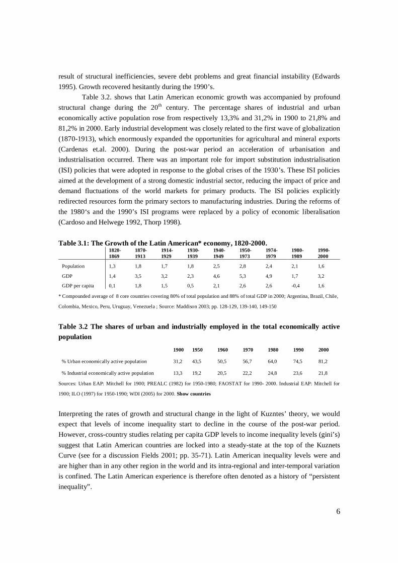
Table 3.2. shows that Latin American economic growth was accompanied by profoundstructural change during the 20th century. The percentage shares of industrial and urbaneconomically active population rose from respectively 13,3% and 31,2% in 1900 to 21,8% and81,2% in 2000. Early industrial development was closely related to the first wave of globalization(1870-1913), which enormously expanded the opportunities for agricultural and mineral exports(Cardenas et.al. 2000). During the post-war period an acceleration of urbanisation andindustrialisation occurred. There was an important role for import substitution industrialisation(ISI) policies that were adopted in response to the global crises of the 1930’s. These ISI policiesaimed at the development of a strong domestic industrial sector, reducing the impact of price anddemand fluctuations of the world markets for primary products. The ISI policies explicitlyredirected resources form the primary sectors to manufacturing industries. During the reforms ofthe 1980‘s and the 1990’s ISI programs were replaced by a policy of economic liberalisation(Cardoso and Helwege 1992, Thorp 1998).

Table 3.1: The Growth of the Latin American* economy, 1820-2000.1820-1869

1870-1913

1914-1929

1930-1939

1940-1949

1950-1973

1974-1979

1980-1989

1990-2000

Population 1,3 1,8 1,7 1,8 2,5 2,8 2,4 2,1 1,6

GDP 1,4 3,5 3,2 2,3 4,6 5,3 4,9 1,7 3,2

GDP per capita 0,1 1,8 1,5 0,5 2,1 2,6 2,6 -0,4 1,6

* Compounded average of 8 core countries covering 80% of total population and 88% of total GDP in 2000; Argentina, Brazil, Chile,

Colombia, Mexico, Peru, Uruguay, Venezuela ; Source: Maddison 2003; pp. 128-129, 139-140, 149-150

Table 3.2 The shares of urban and industrially employed in the total economically activepopulation

1900 1950 1960 1970 1980 1990 2000

% Urban economically active population 31,2 43,5 50,5 56,7 64,0 74,5 81,2

% Industrial economically active population 13,3 19,2 20,5 22,2 24,8 23,6 21,8

Sources: Urban EAP: Mitchell for 1900; PREALC (1982) for 1950-1980; FAOSTAT for 1990- 2000. Industrial EAP: Mitchell for

1900; ILO (1997) for 1950-1990; WDI (2005) for 2000. Show countries

Interpreting the rates of growth and structural change in the light of Kuzntes’ theory, we wouldexpect that levels of income inequality start to decline in the course of the post-war period.However, cross-country studies relating per capita GDP levels to income inequality levels (gini’s)suggest that Latin American countries are locked into a steady-state at the top of the KuznetsCurve (see for a discussion Fields 2001; pp. 35-71). Latin American inequality levels were andare higher than in any other region in the world and its intra-regional and inter-temporal variationis confined. The Latin American experience is therefore often denoted as a history of “persistentinequality”.

7

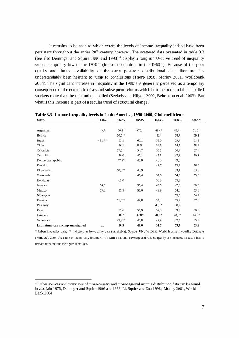
It remains to be seen to which extent the levels of income inequality indeed have beenpersistent throughout the entire 20th century however. The scattered data presented in table 3.3(see also Deininger and Squire 1996 and 1998)11 display a long run U-curve trend of inequalitywith a temporary low in the 1970’s (for some countries in the 1960’s). Because of the poorquality and limited availability of the early post-war distributional data, literature hasunderstandably been hesitant to jump to conclusions (Thorp 1998, Morley 2001, Worldbank2004). The significant increase in inequality in the 1980’s is generally perceived as a temporaryconsequence of the economic crises and subsequent reforms which hurt the poor and the unskilledworkers more than the rich and the skilled (Szekely and Hilgert 2002, Behrmann et.al. 2003). Butwhat if this increase is part of a secular trend of structural change?

Table 3.3: Income inequality levels in Latin America, 1950-2000, Gini-coefficientsWIID 1950's 1960's 1970's 1980's 1990's 2000-2

Argentina 43,7 38,2* 37,2* 42,4* 46,6* 52,3*Bolivia 50,5** 52* 58,7 59,1

Brazil 49,1** 55,1 60,1 59,0 59,4 61,2Chile 46,1 48,5* 54,5 54,5 58,2Colombia 57,8** 54,7 50,8 56,4 57,4Costa Rica 50,0 47,1 45,5 47,1 50,1Dominican republic 47,2* 45,0 48,0 49,0Ecuador 43,7 53,9 56,0El Salvador 50,8** 43,9 53,1 53,8Guatemala 47,4 57,6 54,0 59,8Honduras 62,0 58,8 55,3Jamaica 56,0 55,4 49,5 47,6 38,6Mexico 53,0 55,5 51,6 49,9 54,6 53,0Nicaragua 53,8 54,2Panama 51,4** 49,8 54,4 55,9 57,8Paraguay 45,1* 58,2Peru 57,6 56,9 57,0 49,3 49,3Uruguay 38,8* 42,8* 41,1* 43,7* 44,5*Venezuela 45,3** 40,8 42,9 47,5 45,8

Latin American average unweighted … 50,5 48,6 51,7 53,4 53,9

* Urban inequality only; ** indicated as low-quality data (unreliable); Source: UNU/WIDER, World Income Inequality Database

(WIID 2a), 2005: As a rule of thumb only income Gini’s with a national coverage and reliable quality are included. In case I had to

deviate from the rule the figure is marked.

11 Other sources and overviews of cross-country and cross-regional income distribution data can be foundin a.o. Jain 1975, Deininger and Squire 1996 and 1998, Li, Squire and Zou 1998, Morley 2001, WorldBank 2004.

8

4 An alternative hypothesis

Assessing long run changes in Latin American inequality confronts Kuznets’ theory with somespecific Latin characteristics: 1) a highly skewed distribution of land (and rural income) in thepre-industrial economy, 2) a colonial history of chronic labour scarcity and 3) rapid demographicgrowth and rural-urban migration in the post-war period that leads to unprecedented laboursurpluses.

As stated in section 2, Kuznets theory presupposes that urban income is more unequallydistributed than rural income. Yet, in Latin America rural inequality has been pervasive as a resultof a deeply rooted colonial heritage of land inequality: a bi-polar distribution consisting of a largebase of (native) subsistence-farmers and a confined Creole elite of large landowners. Theexpansion of the rural and mineral resource exports during the 19th century probably hasintensified rural inequality, since most of the rents were accrued by large landowners (Duncanand Rutledge 1977, Kay 2001). A quick comparison of land gini’s in the early 20th century clearlyindicates the exceptional wealth (and power) of the Latin American landowning elites: Argentina1914: 0.80, Brazil 1920: 0,78, Chile 1927: 0.84 and Uruguay 1937: 0.78 versus the USA 1880:0.48, Canada 1931: 0.49, Japan 1909: 0,40, Turkey 1927: 0.56 or even South Africa 1927: 0.62.

Given the high initial levels of rural inequality the shift of landless labourers to the urbaneconomy may have confined rather than enlarged within-sector inequality. Since labour wasrelatively scarce in many Latin American countries, traditional coercive land and labour marketinstitutions were confronted with the competition of urban industries for unskilled rural labour.Atlantic labour migration has been a notable source of new labour in some countries (particularlyArgentina), but this could not prevent an upward trend in real wages in the period 1870-1929 (inthe southern cone countries at least). The increasing bargaining power of unskilled labour in theearly 20th century fuelled social tensions. In the wake of continuous strikes and conflicts overwages and labour conditions, trade unions gained ground and political power (Scobie 1986, Hall1986, XXXX). There are good arguments to believe that after the increasing inequality effect ofthe first export boom, within-sector income inequality declined in a substantial part of LatinAmerican countries. This hypothesis is supported by data indicating an increasing wage-rentratio’s in the period 1914-1960’s in Argentina and Uruguay (Bertola 2001, Bertola andWilliamson 2003).12

In the course of the 20th century urban incomes diverged as a consequence of increasingimbalances in the growth process. One of the key conditions of balanced growth is that theexpansion of the urban sector is sufficient to absorb population growth (Fei and Ranis 1997).From this point of view growth has been balanced in Latin America until the last quarter of the

12 In Mexico labour has been relatively abundant and it is interesting to see that the average wage estimatesof the Primer Census Industrial deviate considerably from the patterns observed in Argentina, Brazil, Chileand Uruguay in 1930.

9

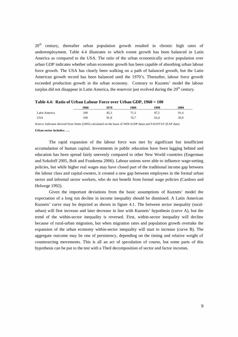
20th century, thereafter urban population growth resulted in chronic high rates ofunderemployment. Table 4.4 illustrates to which extent growth has been balanced in LatinAmerica as compared to the USA. The ratio of the urban economically active population overurban GDP indicates whether urban economic growth has been capable of absorbing urban labourforce growth. The USA has clearly been walking on a path of balanced growth, but the LatinAmerican growth record has been balanced until the 1970’s. Thereafter, labour force growthexceeded production growth in the urban economy. Contrary to Kuznets’ model the laboursurplus did not disappear in Latin America, the reservoir just evolved during the 20th century.

Table 4.4: Ratio of Urban Labour Force over Urban GDP, 1960 = 1001960 1970 1980 1990 2000

Latin America 100 82,3 71,3 87,2 91,4USA 100 81,8 74,7 62,4 50,9

Source: Indicator derived from Smits (2005) calculated on the basis of WDI (GDP data) and FAOSTAT (EAP data)

Urban sector includes: ….

The rapid expansion of the labour force was met by significant but insufficientaccumulation of human capital. Investments in public education have been lagging behind andeducation has been spread fairly unevenly compared to other New World countries (Engermanand Sokoloff 2005, Bolt and Frankema 2006). Labour unions were able to influence wage-settingpolicies, but while higher real wages may have closed part of the traditional income gap betweenthe labour class and capital-owners, it created a new gap between employees in the formal urbansector and informal sector workers, who do not benefit from formal wage policies (Cardoso andHelwege 1992).

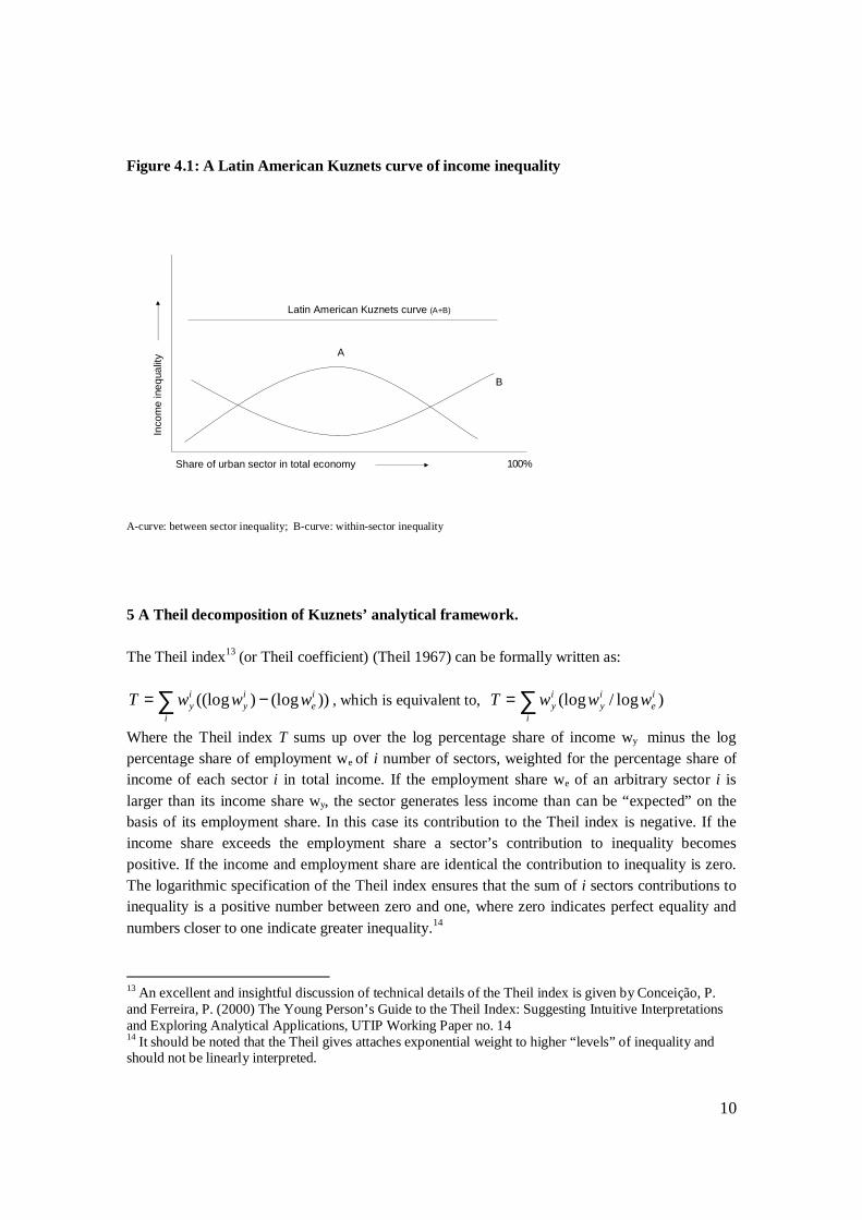
Given the important deviations from the basic assumptions of Kuznets’ model theexpectation of a long run decline in income inequality should be dismissed. A Latin AmericanKuznets’ curve may be depicted as shown in figure 4.1. The between sector inequality (rural-urban) will first increase and later decrease in line with Kuznets’ hypothesis (curve A), but thetrend of the within-sector inequality is reversed. First, within-sector inequality will declinebecause of rural-urban migration, but when migration rates and population growth overtake theexpansion of the urban economy within-sector inequality will start to increase (curve B). Theaggregate outcome may be one of persistency, depending on the timing and relative weight ofcounteracting movements. This is all an act of speculation of course, but some parts of thishypothesis can be put to the test with a Theil decomposition of sector and factor incomes.

10

Figure 4.1: A Latin American Kuznets curve of income inequality

Share of urban sector in total economy

Inco

me

ineq

ualit

y A

B

Latin American Kuznets curve (A+B)

100%

A-curve: between sector inequality; B-curve: within-sector inequality

5 A Theil decomposition of Kuznets’ analytical framework.

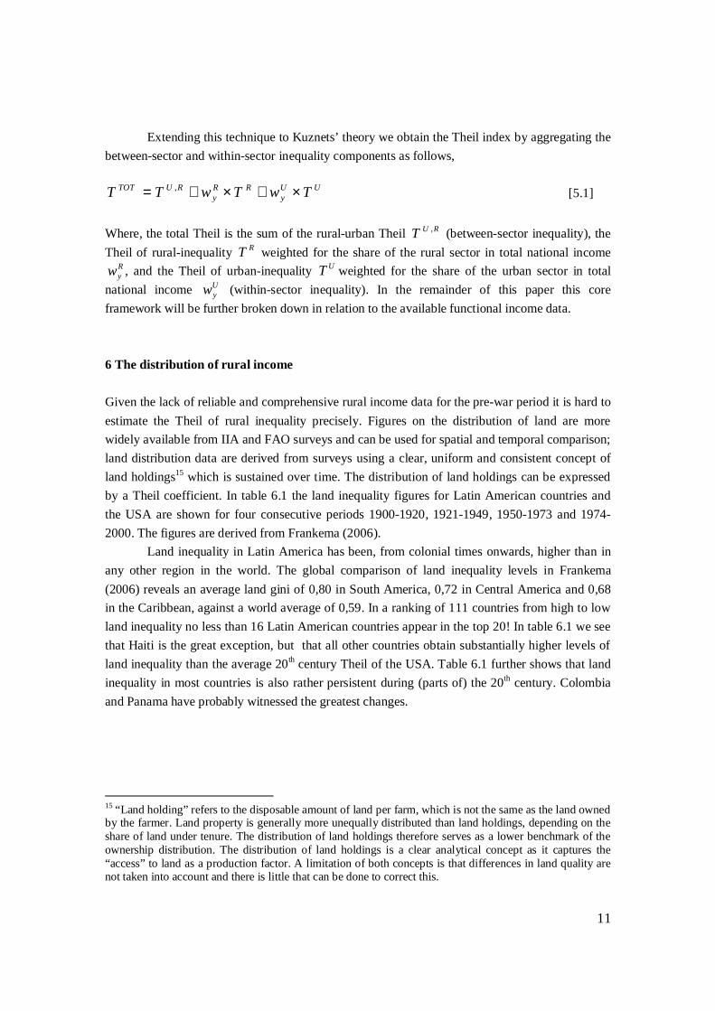
The Theil index13 (or Theil coefficient) (Theil 1967) can be formally written as:

∑ −=i

ie

iy

iy wwwT ))(log)((log , which is equivalent to, ∑=

i

ie

iy

iy wwwT )log/(log

Where the Theil index T sums up over the log percentage share of income wy minus the logpercentage share of employment we of i number of sectors, weighted for the percentage share ofincome of each sector i in total income. If the employment share we of an arbitrary sector i islarger than its income share wy, the sector generates less income than can be “expected” on thebasis of its employment share. In this case its contribution to the Theil index is negative. If theincome share exceeds the employment share a sector’s contribution to inequality becomespositive. If the income and employment share are identical the contribution to inequality is zero.The logarithmic specification of the Theil index ensures that the sum of i sectors contributions toinequality is a positive number between zero and one, where zero indicates perfect equality andnumbers closer to one indicate greater inequality.14

13 An excellent and insightful discussion of technical details of the Theil index is given by Conceição, P.and Ferreira, P. (2000) The Young Person’s Guide to the Theil Index: Suggesting Intuitive Interpretationsand Exploring Analytical Applications, UTIP Working Paper no. 1414 It should be noted that the Theil gives attaches exponential weight to higher “levels” of inequality andshould not be linearly interpreted.

11

Extending this technique to Kuznets’ theory we obtain the Theil index by aggregating thebetween-sector and within-sector inequality components as follows,

UUy

RRy

RUTOT TwTwTT ×+×+= , [5.1]

Where, the total Theil is the sum of the rural-urban Theil RUT , (between-sector inequality), theTheil of rural-inequality RT weighted for the share of the rural sector in total national income

Ryw , and the Theil of urban-inequality UT weighted for the share of the urban sector in total

national income Uyw (within-sector inequality). In the remainder of this paper this core

framework will be further broken down in relation to the available functional income data.

6 The distribution of rural income

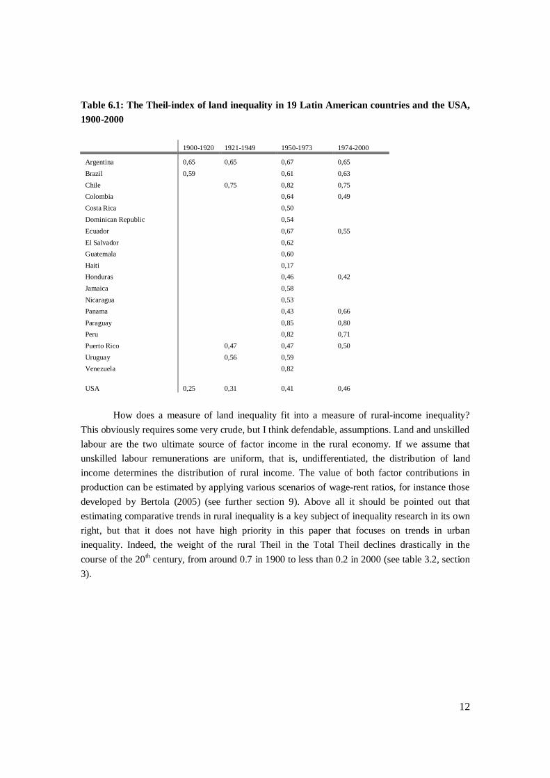
Given the lack of reliable and comprehensive rural income data for the pre-war period it is hard toestimate the Theil of rural inequality precisely. Figures on the distribution of land are morewidely available from IIA and FAO surveys and can be used for spatial and temporal comparison;land distribution data are derived from surveys using a clear, uniform and consistent concept ofland holdings15 which is sustained over time. The distribution of land holdings can be expressedby a Theil coefficient. In table 6.1 the land inequality figures for Latin American countries andthe USA are shown for four consecutive periods 1900-1920, 1921-1949, 1950-1973 and 1974-2000. The figures are derived from Frankema (2006).

Land inequality in Latin America has been, from colonial times onwards, higher than inany other region in the world. The global comparison of land inequality levels in Frankema(2006) reveals an average land gini of 0,80 in South America, 0,72 in Central America and 0,68in the Caribbean, against a world average of 0,59. In a ranking of 111 countries from high to lowland inequality no less than 16 Latin American countries appear in the top 20! In table 6.1 we seethat Haiti is the great exception, but that all other countries obtain substantially higher levels ofland inequality than the average 20th century Theil of the USA. Table 6.1 further shows that landinequality in most countries is also rather persistent during (parts of) the 20th century. Colombiaand Panama have probably witnessed the greatest changes.

15 “Land holding” refers to the disposable amount of land per farm, which is not the same as the land ownedby the farmer. Land property is generally more unequally distributed than land holdings, depending on theshare of land under tenure. The distribution of land holdings therefore serves as a lower benchmark of theownership distribution. The distribution of land holdings is a clear analytical concept as it captures the“access” to land as a production factor. A limitation of both concepts is that differences in land quality arenot taken into account and there is little that can be done to correct this.

12

Table 6.1: The Theil-index of land inequality in 19 Latin American countries and the USA,1900-2000

1900-1920 1921-1949 1950-1973 1974-2000

Argentina 0,65 0,65 0,67 0,65Brazil 0,59 0,61 0,63Chile 0,75 0,82 0,75Colombia 0,64 0,49Costa Rica 0,50Dominican Republic 0,54Ecuador 0,67 0,55El Salvador 0,62Guatemala 0,60Haiti 0,17Honduras 0,46 0,42Jamaica 0,58Nicaragua 0,53Panama 0,43 0,66

Paraguay 0,85 0,80Peru 0,82 0,71Puerto Rico 0,47 0,47 0,50Uruguay 0,56 0,59Venezuela 0,82

USA 0,25 0,31 0,41 0,46

How does a measure of land inequality fit into a measure of rural-income inequality?This obviously requires some very crude, but I think defendable, assumptions. Land and unskilledlabour are the two ultimate source of factor income in the rural economy. If we assume thatunskilled labour remunerations are uniform, that is, undifferentiated, the distribution of landincome determines the distribution of rural income. The value of both factor contributions inproduction can be estimated by applying various scenarios of wage-rent ratios, for instance thosedeveloped by Bertola (2005) (see further section 9). Above all it should be pointed out thatestimating comparative trends in rural inequality is a key subject of inequality research in its ownright, but that it does not have high priority in this paper that focuses on trends in urbaninequality. Indeed, the weight of the rural Theil in the Total Theil declines drastically in thecourse of the 20th century, from around 0.7 in 1900 to less than 0.2 in 2000 (see table 3.2, section3).

13

7 20th century trends in the distribution of manufacturing income

7.1 The development of manufacturing wage inequality

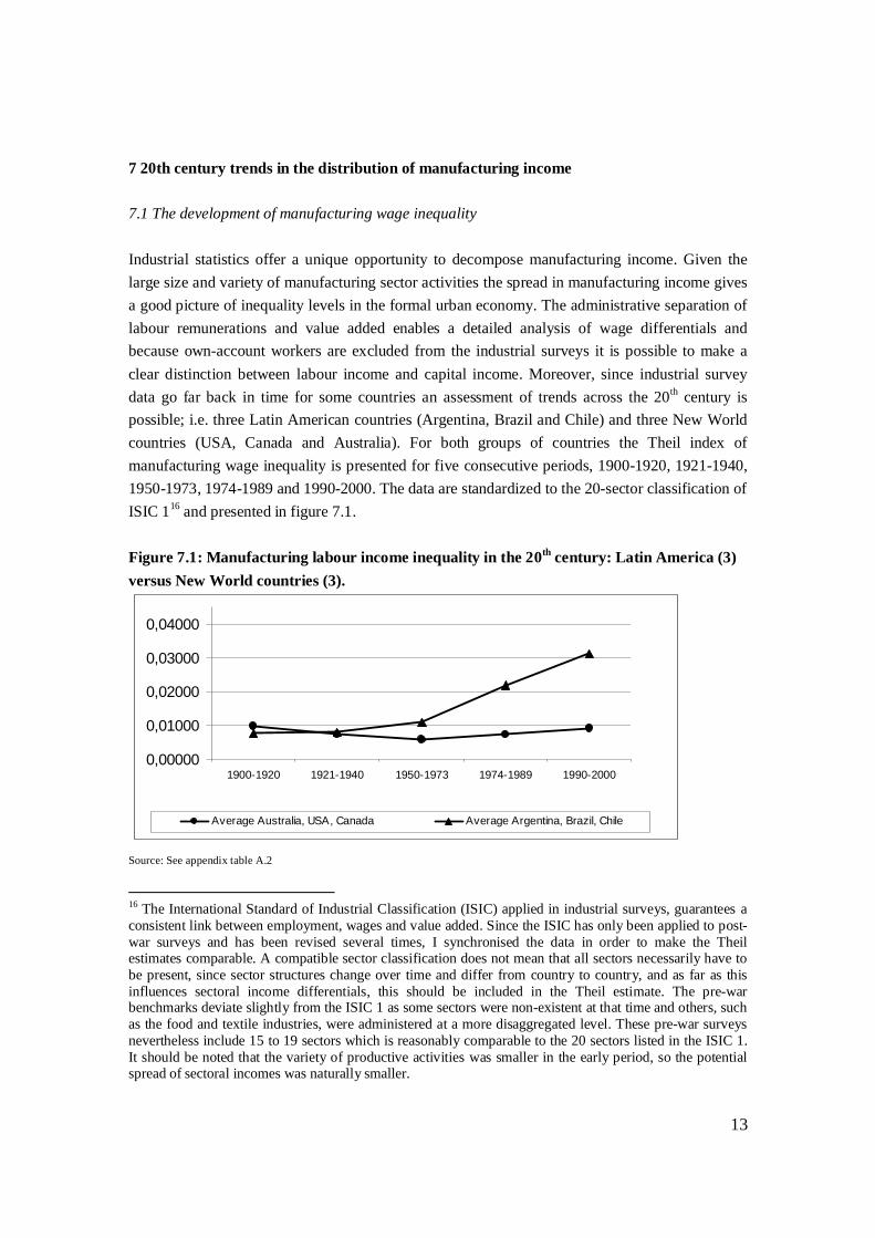
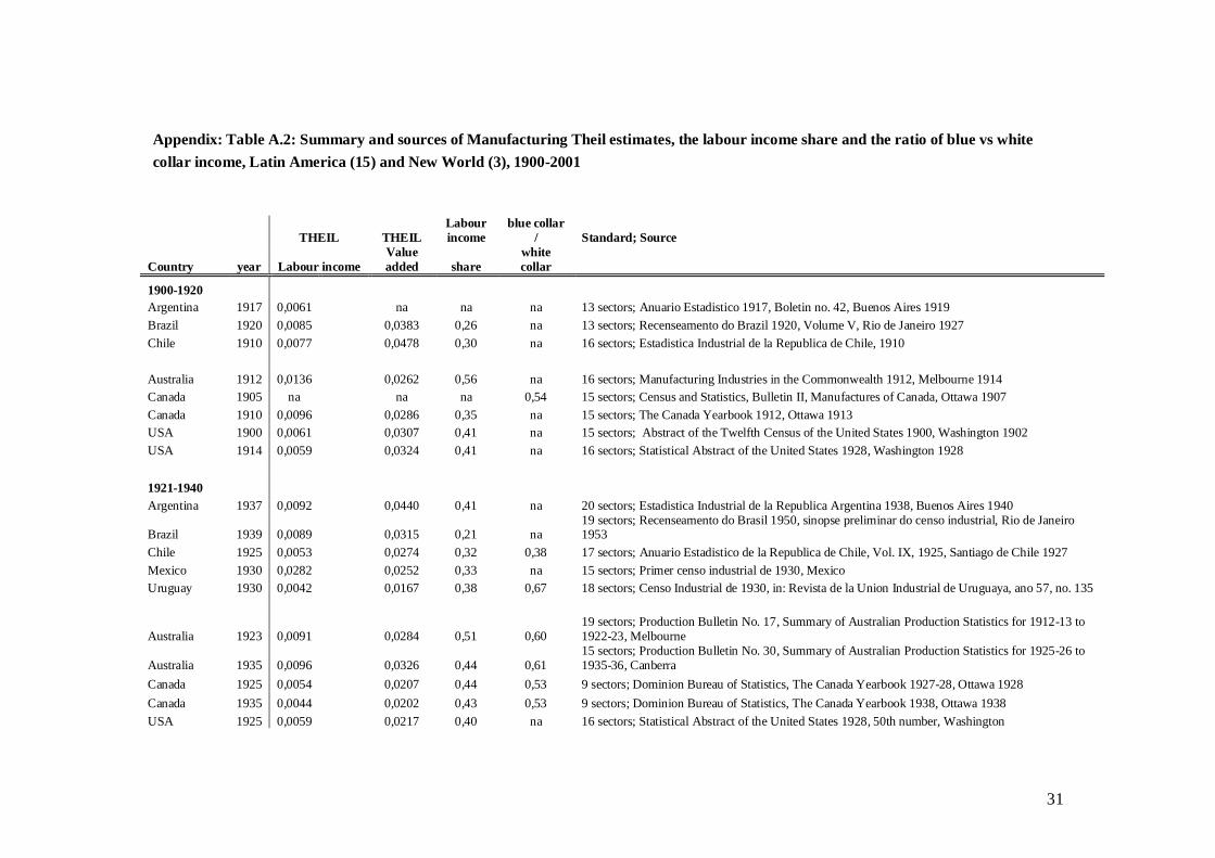
Industrial statistics offer a unique opportunity to decompose manufacturing income. Given thelarge size and variety of manufacturing sector activities the spread in manufacturing income givesa good picture of inequality levels in the formal urban economy. The administrative separation oflabour remunerations and value added enables a detailed analysis of wage differentials andbecause own-account workers are excluded from the industrial surveys it is possible to make aclear distinction between labour income and capital income. Moreover, since industrial surveydata go far back in time for some countries an assessment of trends across the 20th century ispossible; i.e. three Latin American countries (Argentina, Brazil and Chile) and three New Worldcountries (USA, Canada and Australia). For both groups of countries the Theil index ofmanufacturing wage inequality is presented for five consecutive periods, 1900-1920, 1921-1940,1950-1973, 1974-1989 and 1990-2000. The data are standardized to the 20-sector classification ofISIC 116 and presented in figure 7.1.

Figure 7.1: Manufacturing labour income inequality in the 20th century: Latin America (3)versus New World countries (3).

0,00000

0,01000

0,02000

0,03000

0,04000

1900-1920 1921-1940 1950-1973 1974-1989 1990-2000

Average Australia, USA, Canada Average Argentina, Brazil, Chile

Source: See appendix table A.2

16 The International Standard of Industrial Classification (ISIC) applied in industrial surveys, guarantees aconsistent link between employment, wages and value added. Since the ISIC has only been applied to post-war surveys and has been revised several times, I synchronised the data in order to make the Theilestimates comparable. A compatible sector classification does not mean that all sectors necessarily have tobe present, since sector structures change over time and differ from country to country, and as far as thisinfluences sectoral income differentials, this should be included in the Theil estimate. The pre-warbenchmarks deviate slightly from the ISIC 1 as some sectors were non-existent at that time and others, suchas the food and textile industries, were administered at a more disaggregated level. These pre-war surveysnevertheless include 15 to 19 sectors which is reasonably comparable to the 20 sectors listed in the ISIC 1.It should be noted that the variety of productive activities was smaller in the early period, so the potentialspread of sectoral incomes was naturally smaller.

14

Figure 7.1 shows that the pre-war levels of manufacturing wage inequality in the LatinAmerican countries were comparable to the New World countries’ levels and only slightlydiverged until the 1970’s. The increase in wage differentials in the New World after the 1970’s isin line with the established view in the literature.17 Yet, the increase in Latin America was muchmore pronounced than in the New World. The Theil index jumped from ca. 0.01 to 0.03 in LatinAmerica, whereas in the New World the Theil remains just below 0.01. These results support thehypothesis formulated in section 4. If the manufacturing sector in Argentina, Brazil and Chile isrepresentative for the general movement of the income distribution in the urban sector of theLatin American economies, than these figures show that urban inequality has increased ratherthan decreased during the 20th century and that the first half of the 20th century was characterisedby comparatively low levels of urban sector inequality.

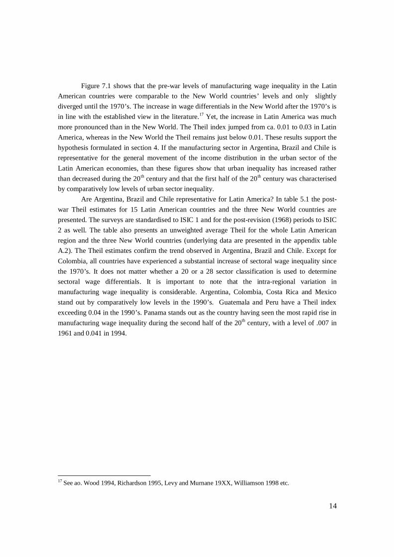
Are Argentina, Brazil and Chile representative for Latin America? In table 5.1 the post-war Theil estimates for 15 Latin American countries and the three New World countries arepresented. The surveys are standardised to ISIC 1 and for the post-revision (1968) periods to ISIC2 as well. The table also presents an unweighted average Theil for the whole Latin Americanregion and the three New World countries (underlying data are presented in the appendix tableA.2). The Theil estimates confirm the trend observed in Argentina, Brazil and Chile. Except forColombia, all countries have experienced a substantial increase of sectoral wage inequality sincethe 1970’s. It does not matter whether a 20 or a 28 sector classification is used to determinesectoral wage differentials. It is important to note that the intra-regional variation inmanufacturing wage inequality is considerable. Argentina, Colombia, Costa Rica and Mexicostand out by comparatively low levels in the 1990’s. Guatemala and Peru have a Theil indexexceeding 0.04 in the 1990’s. Panama stands out as the country having seen the most rapid rise inmanufacturing wage inequality during the second half of the 20th century, with a level of .007 in1961 and 0.041 in 1994.

17 See ao. Wood 1994, Richardson 1995, Levy and Murnane 19XX, Williamson 1998 etc.

15

Table 7.1: A comparison of manufacturing labour income inequality, focusing on the secondhalf of the 20th century: Latin America (15) versus New World countries (3).

1900-1920 1921-1940 1950-1973 1974-1989 1990-2000 1974-1989 1990-2000

20 sectors 20 sectors 20 sectors 28 sectors 28 sectors

Argentina 0,006 0,009 0,006 0,014 0,022 0,015 0,023Bolivia 0,019 0,023 0,038 0,025 0,040Brazil 0,009 0,009 0,013 0,027 0,047 0,027 0,048

Chile 0,008 0,005 0,014 0,025 0,027 0,026 0,029Colombia 0,020 0,015 0,018 0,017 0,019Costa Rica 0,008 0,015 0,018 0,015 0,019Dominican Republic 0,021 0,031 na 0,031 naEcuador 0,016 0,012 0,037 0,014 0,039El Salvador 0,013 0,015 0,028 0,016 0,030Guatemala 0,021 0,030 0,034 0,032 0,046Mexico 0,010 0,010 0,017 0,011 0,018Panama 0,007 0,022 0,040 0,023 0,041

Peru 0,012 0,017 0,047 0,018 0,048Uruguay 0,012 0,015 0,030 0,016 0,031Venezuela 0,013 0,013 0,032 0,014 0,035

Latin America 0,007 0,008 0,014 0,019 0,031 0,020 0,033

Australia 0,014 0,009 0,002 0,003 0,007 0,003 0,008Canada 0,010 0,005 0,007 0,008 0,009 0,008 0,010USA 0,006 0,007 0,007 0,012 0,010 0,013 0,011New World 0,010 0,007 0,006 0,008 0,009 0,008 0,010

Source: See appendix table A.2

7.2 The development of skill-premiums in manufacturing

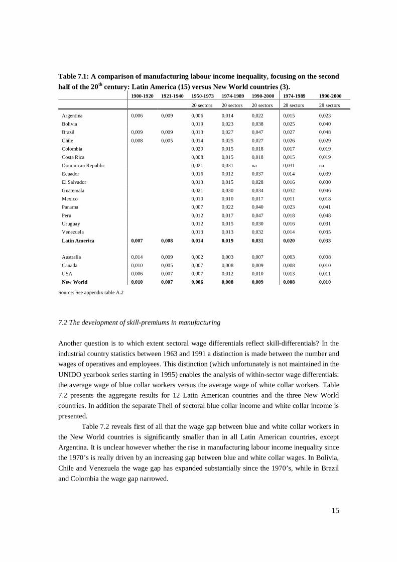
Another question is to which extent sectoral wage differentials reflect skill-differentials? In theindustrial country statistics between 1963 and 1991 a distinction is made between the number andwages of operatives and employees. This distinction (which unfortunately is not maintained in theUNIDO yearbook series starting in 1995) enables the analysis of within-sector wage differentials:the average wage of blue collar workers versus the average wage of white collar workers. Table7.2 presents the aggregate results for 12 Latin American countries and the three New Worldcountries. In addition the separate Theil of sectoral blue collar income and white collar income ispresented.

Table 7.2 reveals first of all that the wage gap between blue and white collar workers inthe New World countries is significantly smaller than in all Latin American countries, exceptArgentina. It is unclear however whether the rise in manufacturing labour income inequality sincethe 1970’s is really driven by an increasing gap between blue and white collar wages. In Bolivia,Chile and Venezuela the wage gap has expanded substantially since the 1970’s, while in Braziland Colombia the wage gap narrowed.

16

Table 7.2: The ratio of average blue collar wages over white collar wages and respectiveTheil indices, Latin America (12) vs New World (3), 1960-1989.

1960's 1970's 1980'sRatio

blue/whiteTheilblue

Theilwhite

Ratioblue/white

theilblue

Theilwhite

Ratioblue/white

theilblue

theilwhite

Argentina 0,77 0,0036 0,0017 0,67 0,0069 0,0119 0,63 0,0128 0,0456Bolivia 0,59 0,0148 0,0318 0,23 0,0117 0,0139Brazil 0,45 0,0093 0,0209 0,47 0,0230 0,0133 0,60 0,0381 0,0301Chile 0,33 0,0240 0,0147 0,38 0,0148 0,0148 0,28 0,0357 0,0175Colombia 0,43 0,0120 0,0094 0,44 0,0141 0,0108 0,56 0,0139 0,0142Ecuador 0,39 0,0100 0,0239 0,44 0,0072 0,0067Guatemala 0,30 0,0134 0,0266 0,39 0,0311 0,0523Mexico 0,49 0,0098 0,0161 0,54 0,0155 0,0089 0,50 0,0081 0,0069Panama 0,47 0,0065 0,0054 0,48 0,0178 0,0089Peru 0,42 0,0093 0,0240 0,41 0,0111 0,0089 0,45 0,0254 0,0182Uruguay 0,43 0,0128 0,0097 0,45 0,0120 0,0104Venezuela 0,40* 0,0107 0,0057 0,17 0,0053 0,0060 0,17 0,0047 0,0056Latin America 0,47 0,0106 0,0135 0,44 0,0131 0,0132 0,43 0,0193 0,0215

Australia 0,77 0,0040 0,0007 0,76 0,0026 0,0023 0,83 0,0048 0,0051Canada 0,72 0,0098 0,0027 0,74 0,0084 0,0022 0,69 0,0125 0,0036USA 0,65 0,0110 0,0032 0,65 0,0107 0,0137 0,64 0,0436 0,0370New World 0,71 0,0083 0,0022 0,72 0,0073 0,0061 0,72 0,0203 0,0152(unweigthed averages)

Source: See appendix table A.2; Venezuela 1971.

The decomposition of the Theil index of manufacturing labour income into blue andwhite collar wages further reveals that the increasing income differentials since the 1970’sapplied to both groups of workers. In the majority of Latin American countries and in all NewWorld countries the average sectoral wages of blue and white collar workers became spread moreunevenly. This means that the observed inequality trend should first and for all be interpreted as aresult of labour income changes between, rather than within manufacturing sectors. In somecountries the sectoral inequality may be driven by an increasing white-collar premium, yet inother countries sectoral inequality increased while the wage gap between blue and white collarworkers narrowed. Mexico, Uruguay and Colombia do not fit in either of these two scenarioshowever (at least until the 1980’s). One real Latin American stylized fact can be maintained:manufacturing sectoral wage differentials in the 1990’s are substantially higher than in the period1950-1973. Colombia is the single exception confirming this rule.

7.3 The labour and capital income share in manufacturing value added

The distribution of labour-capital income is crucial in Kuznets’ explanation of the secular trend ofincome inequality. Since labour income is considered to be more evenly distributed than capitalincome, an increase in the labour-capital income ratio is likely to reduce personal incomeinequality and vice versa. Due to the high capital-intensity of the manufacturing sector the labour-

17

capital income ratio is usually lower than for the total economy including labour-intensive serviceindustries.

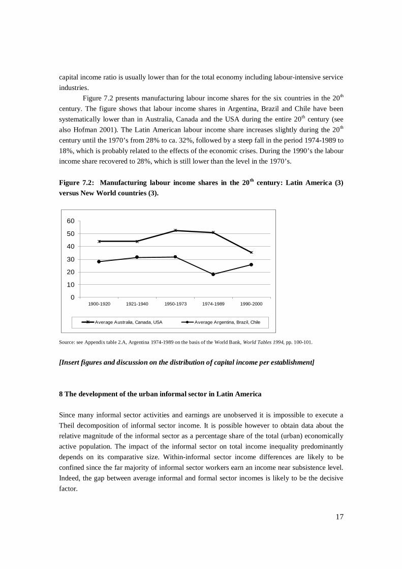
Figure 7.2 presents manufacturing labour income shares for the six countries in the 20th

century. The figure shows that labour income shares in Argentina, Brazil and Chile have beensystematically lower than in Australia, Canada and the USA during the entire 20th century (seealso Hofman 2001). The Latin American labour income share increases slightly during the 20th

century until the 1970’s from 28% to ca. 32%, followed by a steep fall in the period 1974-1989 to18%, which is probably related to the effects of the economic crises. During the 1990’s the labourincome share recovered to 28%, which is still lower than the level in the 1970’s.

Figure 7.2: Manufacturing labour income shares in the 20th century: Latin America (3)versus New World countries (3).

0

10

20

30

40

50

60

1900-1920 1921-1940 1950-1973 1974-1989 1990-2000

Average Australia, Canada, USA Average Argentina, Brazil, Chile

Source: see Appendix table 2.A, Argentina 1974-1989 on the basis of the World Bank, World Tables 1994, pp. 100-101.

[Insert figures and discussion on the distribution of capital income per establishment]

8 The development of the urban informal sector in Latin America

Since many informal sector activities and earnings are unobserved it is impossible to execute aTheil decomposition of informal sector income. It is possible however to obtain data about therelative magnitude of the informal sector as a percentage share of the total (urban) economicallyactive population. The impact of the informal sector on total income inequality predominantlydepends on its comparative size. Within-informal sector income differences are likely to beconfined since the far majority of informal sector workers earn an income near subsistence level.Indeed, the gap between average informal and formal sector incomes is likely to be the decisivefactor.

18

The ILO has devised a simple but consistent method to measure the size of the informalsector on the basis of economically active population data derived from household surveys andpopulation censuses. The method basically involves a classification of own account workers andunpaid family workers into distinct categories. The categories consist of agricultural self-employed (farmers), professional and technical self-employed (i.e. lawyers, ICT-workers etc.),domestic servants and other self-employed. The first two categories are respectively classified asworkers in the traditional agricultural sector (distinct from employees working in modernagricultural enterprises) and urban self-employed in the formal sector. The latter two categoriesare considered to consist of informal sector workers.

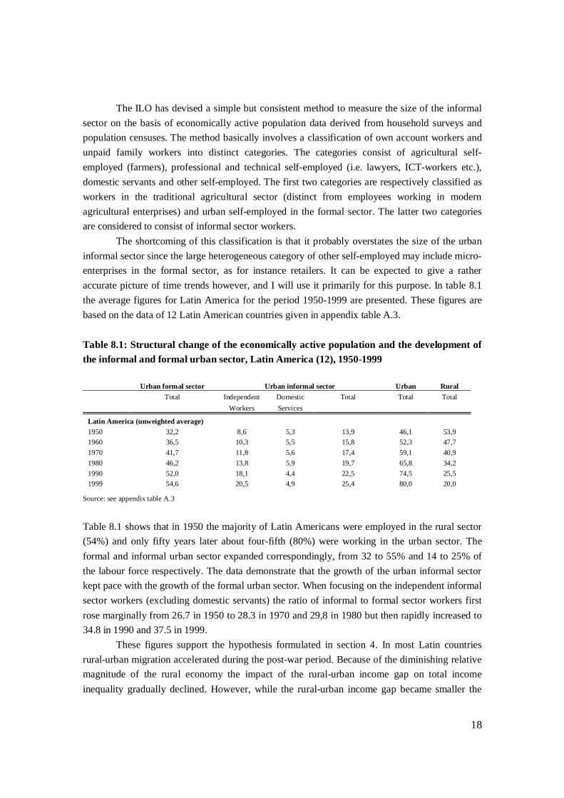
The shortcoming of this classification is that it probably overstates the size of the urbaninformal sector since the large heterogeneous category of other self-employed may include micro-enterprises in the formal sector, as for instance retailers. It can be expected to give a ratheraccurate picture of time trends however, and I will use it primarily for this purpose. In table 8.1the average figures for Latin America for the period 1950-1999 are presented. These figures arebased on the data of 12 Latin American countries given in appendix table A.3.

Table 8.1: Structural change of the economically active population and the development ofthe informal and formal urban sector, Latin America (12), 1950-1999

Urban formal sector Urban informal sector Urban RuralTotal Independent Domestic Total Total Total

Workers Services

Latin America (unweighted average)1950 32,2 8,6 5,3 13,9 46,1 53,91960 36,5 10,3 5,5 15,8 52,3 47,71970 41,7 11,8 5,6 17,4 59,1 40,91980 46,2 13,8 5,9 19,7 65,8 34,21990 52,0 18,1 4,4 22,5 74,5 25,51999 54,6 20,5 4,9 25,4 80,0 20,0

Source: see appendix table A.3

Table 8.1 shows that in 1950 the majority of Latin Americans were employed in the rural sector(54%) and only fifty years later about four-fifth (80%) were working in the urban sector. Theformal and informal urban sector expanded correspondingly, from 32 to 55% and 14 to 25% ofthe labour force respectively. The data demonstrate that the growth of the urban informal sectorkept pace with the growth of the formal urban sector. When focusing on the independent informalsector workers (excluding domestic servants) the ratio of informal to formal sector workers firstrose marginally from 26.7 in 1950 to 28.3 in 1970 and 29,8 in 1980 but then rapidly increased to34.8 in 1990 and 37.5 in 1999.

These figures support the hypothesis formulated in section 4. In most Latin countriesrural-urban migration accelerated during the post-war period. Because of the diminishing relativemagnitude of the rural economy the impact of the rural-urban income gap on total incomeinequality gradually declined. However, while the rural-urban income gap became smaller the

19

urban income gap opened up. The crucial turn in the development of the informal sector has to belocated somewhere in the late 1970’s and early 1980’s, since from that time onwards the informalsector expanded more rapidly than the urban economy as a whole.

9 Accounting total inequality in the 20th century: An inverted Kuznets curve?

This section presents the aggregate trends in the comparative development of the functionalincome distribution in the 20th century for Argentina, Brazil and Chile. The USA serves as acomparative benchmark. The four main components of the functional income distribution, i.e.rural inequality, rural-urban inequality, urban informal-formal inequality and urban formalinequality are tied together in the comprehensive framework of the total Theil index as presentedin section 5. After the formal derivation of the framework and its assumptions the empiricalresults will be presented.

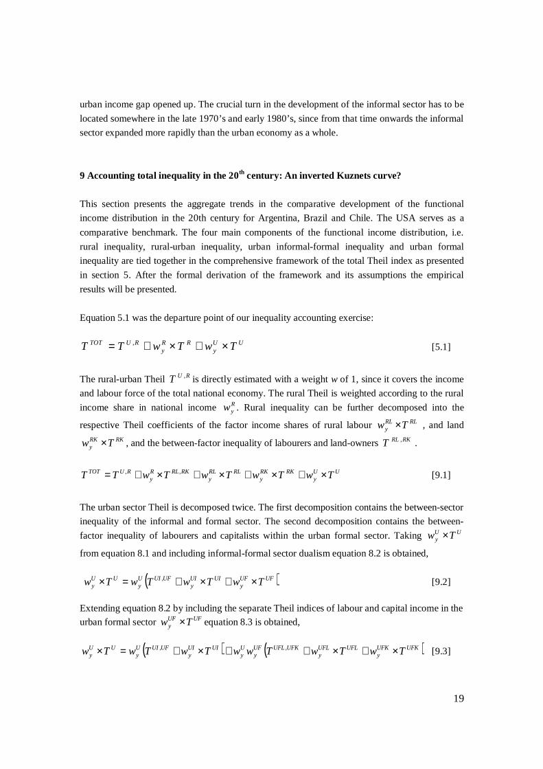
Equation 5.1 was the departure point of our inequality accounting exercise:

UUy

RRy

RUTOT TwTwTT ×+×+= , [5.1]

The rural-urban Theil RUT , is directly estimated with a weight w of 1, since it covers the incomeand labour force of the total national economy. The rural Theil is weighted according to the ruralincome share in national income R

yw . Rural inequality can be further decomposed into the

respective Theil coefficients of the factor income shares of rural labour RLRLy Tw × , and land

RKRKy Tw × , and the between-factor inequality of labourers and land-owners RKRLT , .

UUy

RKRKy

RLRLy

RKRLRy

RUTOT TwTwTwTwTT ×+×+×+×+= ,, [9.1]

The urban sector Theil is decomposed twice. The first decomposition contains the between-sectorinequality of the informal and formal sector. The second decomposition contains the between-factor inequality of labourers and capitalists within the urban formal sector. Taking UU

y Tw ×

from equation 8.1 and including informal-formal sector dualism equation 8.2 is obtained,

( )UFUFy

UIUIy

UFUIUy

UUy TwTwTwTw ×+×+=× , [9.2]

Extending equation 8.2 by including the separate Theil indices of labour and capital income in theurban formal sector UFUF

y Tw × equation 8.3 is obtained,

( ) ( )UFKUFKy

UFLUFLy

UFKUFLUFy

Uy

UIUIy

UFUIUy

UUy TwTwTwwTwTwTw ×+×++×+=× ,, [9.3]

20

Substituting 8.3 into 8.1 gives the comprehensive Theil framework,

( )( )

( )UFKUFKy

UFLUFLy

UFKUFLUFy

Uy

UIUIy

UFUIUy

RKRKy

RLRLy

RKRLRy

RUTOT

TwTwTww

TwTw

TwTwTwTT

×+×++

×++

×+×+×+

=

,

,

,

,

[9.4]

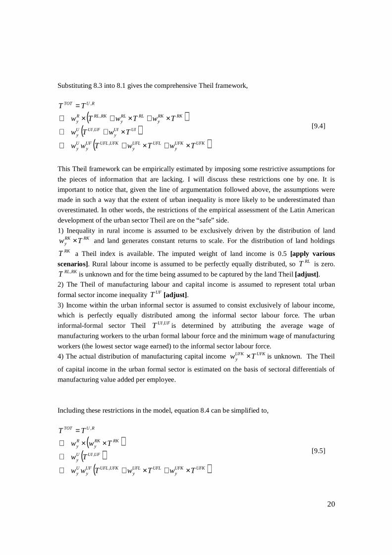
This Theil framework can be empirically estimated by imposing some restrictive assumptions forthe pieces of information that are lacking. I will discuss these restrictions one by one. It isimportant to notice that, given the line of argumentation followed above, the assumptions weremade in such a way that the extent of urban inequality is more likely to be underestimated thanoverestimated. In other words, the restrictions of the empirical assessment of the Latin Americandevelopment of the urban sector Theil are on the “safe” side.1) Inequality in rural income is assumed to be exclusively driven by the distribution of land

RKRKy Tw × and land generates constant returns to scale. For the distribution of land holdingsRKT a Theil index is available. The imputed weight of land income is 0.5 [apply various

scenarios]. Rural labour income is assumed to be perfectly equally distributed, so RLT is zero.RKRLT , is unknown and for the time being assumed to be captured by the land Theil [adjust].

2) The Theil of manufacturing labour and capital income is assumed to represent total urbanformal sector income inequality UFT [adjust].3) Income within the urban informal sector is assumed to consist exclusively of labour income,which is perfectly equally distributed among the informal sector labour force. The urbaninformal-formal sector Theil UFUIT , is determined by attributing the average wage ofmanufacturing workers to the urban formal labour force and the minimum wage of manufacturingworkers (the lowest sector wage earned) to the informal sector labour force.4) The actual distribution of manufacturing capital income UFKUFK

y Tw × is unknown. The Theil

of capital income in the urban formal sector is estimated on the basis of sectoral differentials ofmanufacturing value added per employee.

Including these restrictions in the model, equation 8.4 can be simplified to,

( )( )

( )UFKUFKy

UFLUFLy

UFKUFLUFy

Uy

UFUIUy

RKRKy

Ry

RUTOT

TwTwTww

Tw

TwwTT

×+×++

+

××+

=

,

,

,

[9.5]

21

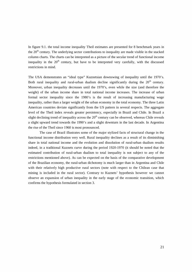
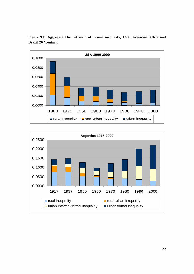
In figure 9.1. the total income inequality Theil estimates are presented for 8 benchmark years inthe 20th century. The underlying sector contributions to inequality are made visible in the stackedcolumn charts. The charts can be interpreted as a picture of the secular trend of functional incomeinequality in the 20th century, but have to be interpreted very carefully, with the discussedrestrictions in mind.

The USA demonstrates an “ideal type” Kuznetsian downswing of inequality until the 1970’s.Both rural inequality and rural-urban dualism decline significantly during the 20th century.Moreover, urban inequality decreases until the 1970’s, even while the size (and therefore theweight) of the urban income share in total national income increases. The increase of urbanformal sector inequality since the 1980’s is the result of increasing manufacturing wageinequality, rather than a larger weight of the urban economy in the total economy. The three LatinAmerican countries deviate significantly from the US pattern in several respects. The aggregatelevel of the Theil index reveals greater persistency, especially in Brazil and Chile. In Brazil aslight declining trend of inequality across the 20th century can be observed, whereas Chile revealsa slight upward trend towards the 1990’s and a slight downturn in the last decade. In Argentinathe rise of the Theil since 1960 is most pronounced.

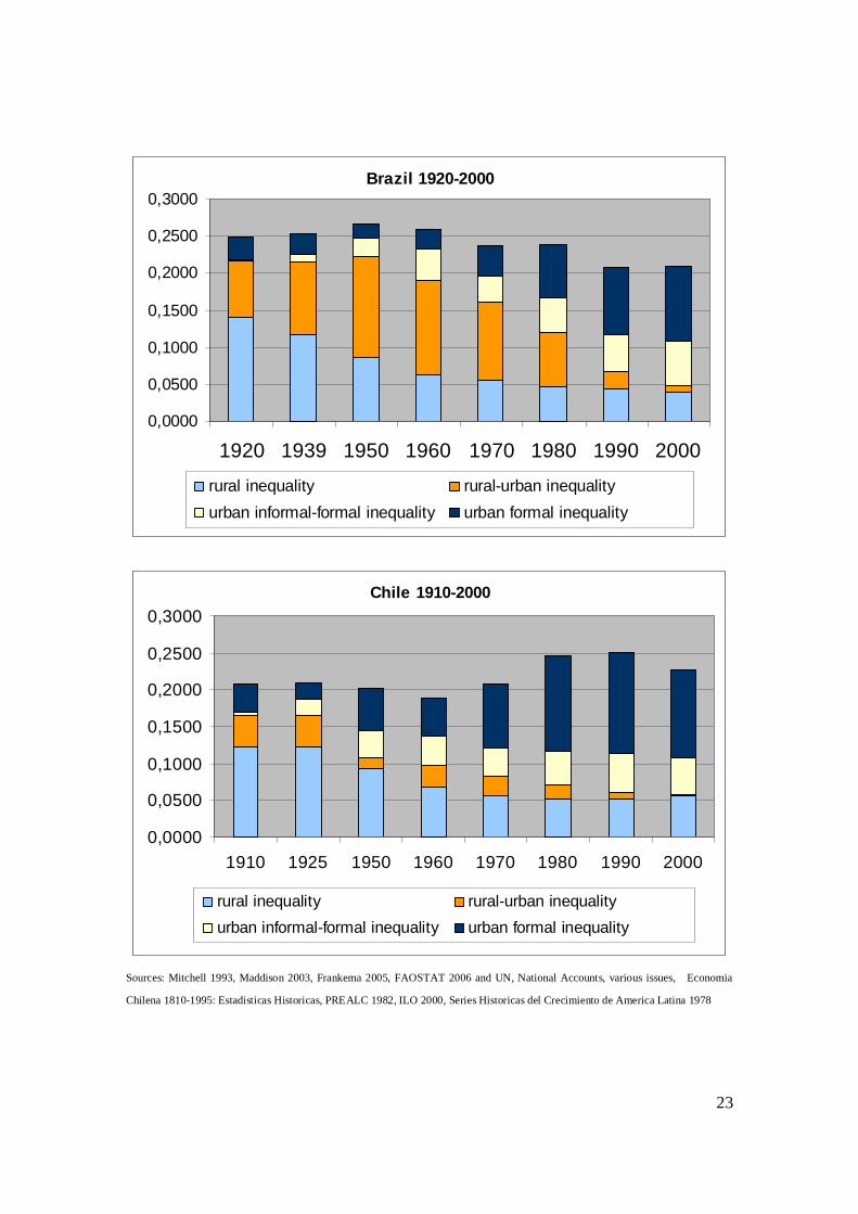
The case of Brazil illustrates some of the major stylized facts of structural change in thefunctional income distribution very well. Rural inequality declines as a result of its diminishingshare in total national income and the evolution and dissolution of rural-urban dualism resultsindeed, in a traditional Kuznets curve during the period 1920-1970 (it should be noted that theestimated contribution of rural-urban dualism to total inequality is not subject to any of therestrictions mentioned above). As can be expected on the basis of the comparative developmentof the Brazilian economy, the rural-urban dichotomy is much larger than in Argentina and Chilewith their relatively high productive rural sectors (note with respect to the Chilean case thatmining is included in the rural sector). Contrary to Kuznets’ hypothesis however we cannotobserve an expansion of urban inequality in the early stage of the economic transition, whichconfirms the hypothesis formulated in section 3.

22

Figure 9.1: Aggregate Theil of sectoral income inequality, USA, Argentina, Chile andBrazil, 20th century.

USA 1900-2000

0,0000

0,0200

0,0400

0,0600

0,0800

0,1000

1900 1925 1950 1960 1970 1980 1990 2000

rural inequality rural-urban inequality urban inequality

Argentina 1917-2000

0,0000

0,0500

0,1000

0,1500

0,2000

0,2500

1917 1937 1950 1960 1970 1980 1990 2000

rural inequality rural-urban inequalityurban informal-formal inequality urban formal inequality

23

Brazil 1920-2000

0,0000

0,0500

0,1000

0,1500

0,2000

0,2500

0,3000

1920 1939 1950 1960 1970 1980 1990 2000

rural inequality rural-urban inequalityurban informal-formal inequality urban formal inequality

Chile 1910-2000

0,0000

0,0500

0,1000

0,1500

0,2000

0,2500

0,3000

1910 1925 1950 1960 1970 1980 1990 2000

rural inequality rural-urban inequalityurban informal-formal inequality urban formal inequality

Sources: Mitchell 1993, Maddison 2003, Frankema 2005, FAOSTAT 2006 and UN, National Accounts, various issues, Economia

Chilena 1810-1995: Estadisticas Historicas, PREALC 1982, ILO 2000, Series Historicas del Crecimiento de America Latina 1978

24

The rural-urban income gap in Argentina and Chile probably has reached its zenith in an earlierstage during the second half of the 19th century, since at the start of 20th century rural incomeamounted to approximately 25% and 35% in total income in both countries respectively. In bothcountries the contribution of urban inequality to total inequality remains confined until the1960’s. Urban inequality just expands beyond the USA levels during the last quarter of thecentury. A substantial part of urban inequality is caused by the growing productivity gap betweeninformal and formal urban activities. Equally important is the sectoral inequality within the urbanformal sector.

It should be pointed out that these figures probably underestimate the comparative impactof formal urban sector inequality and informal-formal sector dualism. It is assumed that everyemployee earns a share of capital income in line with its relative labour productivity. In fact,capital income is much less evenly distributed and a large part of it ends up in the hands of asmall minority. Temporal changes in the unobserved distribution of capital income therefore are amain candidate to revise the charts presented here. The income gap between the informal andformal urban sector is also based on rather conservative estimates.

The most interesting part of this analysis, in my view, concerns the perceived potentialturning point in the trend of income inequality, which I speculatively situated in the 1970’s. Thisprediction is not exactly represented by the charts in figure 8.1. Brazil still awaits such a turningpoint. In Argentina and Chile this turning point is shown quite convincingly however, but earlier,around 1960 already. These results correspond quite well to the income Gini’s presented in table3.3 (section 3). These scenarios thus indicate what the potential impact of long run structuralchange has been on the secular trend of personal income inequality and they are in line withliterature that tentatively suggests that from the early 20th century onwards until the 1970’sincome inequality has been declining in Latin America (Bertola 2001, Thorp 1998).

9 Conclusion

Kuznets argued that the economic transition from a traditional rural into a modern urban economyeventually results, after an upswing in the early phase of industrialisation, in structurally lowerlevels of personal income inequality (inverted U-curve). However, in spite of various phases ofstrong economic growth and profound structural change such a sustained structural decline inincome inequality has not taken place in Latin America. The question addressed in this paper ishow structural change can account for the apparent “persistency” in Latin American personalincome inequality over time. A Theil decomposition is used to investigate long run changes in thefunctional income distribution of 20th century Latin America.

The answer I put forward has two dimensions. First, the Theil decomposition indeed underlines atendency towards persistency because of a well observable “overtaking inequality” effect. Theinitial expansion of rural-urban sector dualism has been countered by relatively low levels of

25

within-sector inequality in the urban economy in the early 20th century. In the post-war period,urban inequality rapidly overtakes the declining rural-urban income gap. A rapid increase inmanufacturing productivity and wage differentials and an acceleration in the expansion of theurban informal sector pushed urban inequality beyond pre-modern levels. The pre-modern levelsappear to be very well comparable to major New World countries as Australia, Canada and theUSA, but deviated from the ideal type Kuznetsian path since the 1970’s.

Second, a tendency of persistency, to a certain extent also draws a misleading picture ofthe Latin American distributional experience. The graphs in the previous section show that thecomposition of the income distribution has been transformed profoundly during the 20th century,more than ever before. The functional income approach is probably the only feasible approach toassess the major shifts in personal income inequality levels before the 1970’s, which so farremain largely unobserved. Combining Kuznetsian logic with the Theil estimates of sector andfactor income presented in this paper, support the idea that the secular trend in 20th centuryincome inequality in Latin America corresponds to a reversed Kuznets curve. Of course it shouldbe stressed, once again, that this result is based on several crude assumptions regarding lackingobservations.

In any case it is impossible to escape the conclusion that the traditional type of ruralinequality characteristic of the colonial and 19th century economy has become less influential,whereas meanwhile, the modern type of urban inequality has remained confined until at least thetwo first post-war decades. Although important dimensions of urban inequality (service andpublic sector inequality for instance) and capital income inequality have been left untouched inthis paper, there is no evidence that the recent expansion of urban inequality since the 1970’s hasbeen preceded in any period between 1870 and 1979. In other words, the timing of the trade-offbetween the two types of economic dualism supports a U-curve, rather than an inverted U-curvetrend in the 20th century.

Perhaps most important is that the results show that the “traditional” Kuznetsianframework, focusing on functional income distribution, earns a prominent place in the inequalityresearch agenda. This approach guarantees an extension of potential data sources, in combinationwith an appropriate analytical tool (Theil index). Kuznets analytical framework offers theopportunity to work with a comprehensive comparative perspective on income inequality acrosscountries and over time. Such an approach, I am convinced, will ultimately reveal the majorimportance of long run secular trends as an “ultimate cause” of inequality.

References

Acemoglu, D., Robinson, J.A. (2006) The Economic Origins of Dictatorship and Democracy, CambridgeUniversity Press: New York

Acemoglu, D., Johnson S. and Robinson, J.A. (2001) The Colonial Origins of Comparative Development:An Empirical Investigation, American Economic Review, Vol. 91, no. 5, pp. 1369-1401

26

Acemoglu, D. (2002) Directed Technological Change, Review of Economic Studies, Vol. 69, no. 4, pp. 781-809

Acemoglu, D. (2003) Cross-Country Inequality Trends, The Economic Journal, Vol. 113, no. 485, pp. 121-149

Ahluwahlia, M.S. (1976a) Income Distribution and Development: Some Stylized facts, The AmericanEconomic Review, Vol. 66, no. 2, pp. 128-135

Ahluwahlia, M.S. (1976b) Inequality, poverty and Development, Journal of Development Economics, Vol.3, no. 4, pp. 307-342

Alesina, A. and Rodrik, D. (1994) Distributive Politics and Economic Growth, The Quarterly Journal ofEconomics, Vol. 109, no. 2, pp. 465-90

Anand, S. and Kanbur, S.M.R. (1993) The Kuznets Process and the Inequality-Development Relationship,Journal of Development Economics, Vol. 40, no. 1, pp. 25-52

Atkinson, A.B. (1997) Bringing Income Distribution in from the Cold, The Economic Journal, Vol. 107,no. 441, pp. 297-321

Barro, R.J. (2000) Inequality and Growth in a Panel of Countries, Journal of Economic Growth, Vol. 5, no.1, pp. 5-32

Behrman, J.R., Birdsall, N. and Szekely, M. (2003) New Data, New Doubts: Revisiting “Aid, Policies, andGrowth” in Latin America, Center for Global Development, Working Paper Number 29

Benjamin, D. and Brandt, L. (1997) Land, Factor Markets, and Inequality in rural China: HistoricalEvidence, Explorations in Economic History, Vol. 34, no. 4, pp. 460-494.

Bertola, L. (2001) Income Distribution and the Kuznets Curve: Argentina and Uruguay since the 1870’s,presented at the International Workshop on “Modern Economic Growth and Distribution in Asia, LatinAmerica, and the European Periphery: A Historical National Accounts Approach, 16-18 March: Tokyo

Bertola, L. and Williamson, J.G. (2003) Globalization in Latin America before 1940. NBER WorkingPaper 9687: Cambridge MA

Birdsall, N. and Londono, J.L. (1997) Asset Inequality Matters: An Assessment of the World Bank’sApproach to Poverty Reduction, The American Economic Review, Vol. 87, no. 2, pp. 32-37

Bourguignon, F. and Morrisson, C. (1998) Inequality and Development: The Role of Dualism, Journal ofDevelopment Economics, Vol. 57, no. 2, pp. 233-257

Cardenas, E., Ocampo, J.A. and Thorp, R. (2000) Introduction. The Export Age: The Latin AmericanEconomies in the late Nineteenth and Early Twentieth Centuries, in: An Economic History of Twentieth-Century Latin America, Volume 1: The Export Age: The Latin American Economies in the late Nineteenthand Early Twentieth Centuries, Plagrave: New York

Cardoso, E. and Helwege, A. (1992) Latin America’s Economy. Diversity, Trends, and Conflicts, The MITPress: Cambridge, MA, London

Conceição, P. and Ferreira, P. (2000) The Young Person’s Guide to the Theil Index: Suggesting IntuitiveInterpreatations and Exploring Analytical Applications, UTIP Working Paper no. 14

Deininger, K. and Squire, L. (1996) A New Data Set Measuring Income Inequality, The World BankEconomic Review, Vol. 10, no. 3, pp. 565-591

27

Deininger, K. and Squire, L. (1998) New ways of looking at old issues: inequality and growth, Journal ofDevelopment Economics, Vol. 57, no. 2, pp. 259-287

De Soto, H. (2000) The Mystery of Capital. Why Capitalism Triumphs in the West and Fails EverywhereElse, Bantam Press: London

Dumke, R. (1991) Income Inequality and Industrialization in Germany, 1850-1913: The KuzentsHypothesis re-examined, in: Brenner, Y.S., Kaelble, H . and Thomas, M. (eds.), Income Distribution inHistorical Perspective, Cambridge University Press, pp. 117-148

Duncan, K. and Rutledge, I. (1977) Introduction: Patterns of Agrarian Capitalism in Latin America, in:Duncan, K. and Rutledge, I., eds., Land and Labour in Latin America. Essays on the Development ofAgrarian Capitalism in the Nineteenth and Twentieth Centuries, Cambridge University Press: London,New York

Easterly, W. and Levine, R. (2003) Tropics, Germs, and Crops: How Endowments influence EconomicDevelopment, Journal of Monetary Economics, Vol. 50, pp. 3-39

Edwards, S. (1995) Crises and Reform in Latin America. From Despair to Hope, World Bank, OxfordUniversity Press: New York

Engerman, S.L. and Sokoloff, K.L. (2005) Colonialism, Inequality and Long-Run Paths of Development,NBER Working Paper 11057, Cambridge MA

Fei, J.C.H. and Ranis, G. (1997) Growth and Development from an Evolutionary Perspective, BlackwellPublishers: Oxford, Malden MA

Fields, G.S. (1980) Poverty, Inequality, and Development, Cambridge University Press: Cambridge, MA,London

Fields, G.S. (2001) Distribution and Development. A New Look at the Developing World, The MIT Press:Cambridge, MA, London

Forbes, K.J. (2000) A Rassessment of the Relationship between Inequality and Growth, The AmericanEconomic Review, Vol. 90, no. 4, pp. 869-887

Frankema, E.H.P. (2006) The Colonial Origins of Inequality: Exploring the Causes and Consequences ofLand Distribution, Groningen Growth and Development Centre, Research Memorandum GD-81,www.ggdc.net

Galor, O., Zeira, J. (1993) Income Distribution and Macroeconomics, The Review of Economic Studies,Vol. 60, no. 1, pp. 35-52

Gylfason, T. and Zoega, G. (2003) Education, Social Equality and Economic Growth: A View of theLandscape, CESifo Working paper no. 876

Hall, M.M. (1986) The Urban Working Class and Early Latin American Labour Movements, 1880-1930, in:Bethel, L. ed., The Cambridge History of Latin America. Volume IV, c. 1870-1930, Cambridge UniversityPress: London, New York

Hofman, A.A. (2001) Economic Growth, Factor Shares and Income Distribution in latin america in theTwentieth Century, presented at the International Workshop on “Modern Economic Growth and Distributionin Asia, Latin America, and the European Periphery: A Historical National Accounts Approach, 16-18 March:Tokyo

28

Jain, S. (1975) Size Distribution of Income. A Compilation of Data, World Bank: Washington D.C.

de Janvry, A. and Sadoulet, E. (2000) Growth and Poverty and Inequality in Latin-america: A causal Analysis,1970-1994, Review of Income and Wealth, 46(3), pp. 267-288.

Kaelble, H. and Thomas, M. (1991) Introduction, in: Brenner, Y.S., Kaelble, H . and Thomas, M. (eds.),Income Distribution in Historical Perspective, Cambridge University Press, pp. 1-56

Kay, C. (2001) Asia’s and Latin America’s Development in Comparative Perspective: Landlords, Peasantsand Industrialization, ISS Working Paper Series, No. 336

Krugman, P.R. (1995) Growing World Trade: Causes and Consequences, Brookings Papers on EconomicActivity, Vol. 1, pp. 327-362

Kuznets, S. (1955) Economic Growth and Income Inequality, in: The American Economic Review, 1,Volume XLV

Kuznets, S. (1957) Quantative Aspects of the Economic growth of Nations II. Industrial Distribution ofNational Product and Labor Force, Economic devlopment and Cultural Change, 4, supplement to volumeV, pp. 1-111

Kuznets, S. (1966) Modern Economic Growth. Rate, Structure and Spread, Yale University Press: NewHaven, Connecticut

Kuznets, S. (1979) Growth, Population and Income Distribution. Selected Essays, W.W. Norton &Company: New York, London

Leamer, E.E. (2000) What’s the Use of Factor Content?, Journal of International Economics, Vol. 50, pp.17-50

Leamer, E.E., Maul, H., Rodriguez, S., Schott, P.K. (1999) Does natural resource abundance increase LatinAmerican income inequality ? Journal of Development Economics, Vol. 59, pp. 3-41

Levy, F. and Murnane, R.J. (1992) U.S. Earnings Levels and Earnings Inequality: A Review of RecentTrends and Proposed Explanations, Journal of Economic Literature, Vol. 30, no. 3, pp. 1333-1381

Lewis, W.A. (1954) Economic Development with Unlimited Supplies of labor, The Manchester School ofEconomic and Social Studies, Vol. 22, pp. 139-191

Li, H., Squire, L., Zou, H. (1998) Explaining International and Intertemporal Variations in IncomeInequality, The Economic Journal 108, January, 26-43

Lindert, P.H. and Williamson, J.G. (1980) American Inequality: A Macroeconomic History, New York

Lindert, P.H. and Williamson, J.G. (1985) Growth, Equity, and History, Explorations in Economic History,Vol. 22, no. 4, pp. 341-377

Maddison, A. (2003) The World Economy: Historical Statistics, OECD: Paris

Mariscal, E. and Sokoloff, K.L. (2000) Schooling, Suffrage, and Inequality in the Americas, 1800-1945, in:S. Haber (ed.) Political Institutions and Economic Growth in Latin America. Essays in Policy, History, andPolitical Economy, Hoover Institution Press: Stanford, California

Morley, S.A. (2001) The income distribution in Latin America and The Caribbean, ECLAC: Santiago,Chile

29

Morrisson, C. (2000) Historical Perspectives on Income Distribution: The Case of Europe, in: Atkinson,A.B. and Bourguignon, F. (eds), Handbook of Income Distribution (Chapter 4), North-Holland:Amsterdam, Boston

Paukert, F. (1973) Income Distribution at Different Levels of Development: A Survey of the Evidence,ILO, International Labour Review, Vol. 108, no. 2-3, pp. 97-125

Persson, T. and Tabellini, G. (1992) Growth, distribution and politics, European Economic Review, Vol.36, pp. 593-602

Richardson, J.D. (1995) Income Inequality and Trade: How to Think, What to Conclude, Journal ofEconomic Perspectives, Vol. 9, No. 3, pp. 33-55

Robinson, S. (1976) A Note on the U Hypothesis relating Income Inequality and Economic Development,The American Economic Review, Vol. 66, pp. 437-440

Scobie, J.R. (1986) The Growth of Latin American Cities, 1870-1930, in: Bethel, L. ed., The CambridgeHistory of Latin America. Volume IV, c. 1870-1930, Cambridge University Press: London, New York

Smits, J.P. (2005) Long-Run African Growth, 1910-2000: An Anlysis Based on a Broad Capital Concept,Paper presented at the Conference of the European Historical Economics Society, September 2005, Istanbul

Soltow, L. and van Zanden, J.L. (1998) Income and wealth inequality in the Netherlands, 16th-20th century,Het Spinhuis: Amsterdam

Spilimbergo, A., Londono, J.L. and Szekely, M. (1999) Income Distribution, Factor Endowments , andTrade Openness, Journal of Development Economics, Vol. 59, pp. 77-101

Szekely, M. and Hilgert M. (2002) Inequality in Latina America during the 1990’s, in: Freeman, R.B., ed.,Inequality Around the World, Macmillan: London

Theil, H. (1967) Economics and Information Theory, Rand McNally and Company: Chigaco

Thorp, R. (1998) Progress, Poverty and Exclusion. An Economic History of Latin america in the 20thCentury, Inter-American Development Bank, New York, The Johns Hopkins University Press: Baltimore,Maryland

Williamson, J.G. (1991) British Inequality during the Industrial Revolution: Accounting for the KuznetsCurve, in: Brenner, Y.S., Kaelble, H . and Thomas, M. (eds.), Income Distribution in HistoricalPerspective, Cambridge University Press, pp. 57-75

Wood, A. (1994) North-South Trade, Employment and Inequality. Changing Fortunes in a Skill-DrivenWorld, Clarendon Press: Oxford

Van Zanden, J.L. (1995) Tracing the Beginning of the Kuznets Curve: Western Europe during the EarlyModern Period, Economic History Review, Vol. XLVIII, no. 4, pp. 643-664

Zhang, X and Zhang, K.H. (2003) How does globalisation affect regional inequality in a developingcountry? Evidence from China. Journal of Development Studies, Vol. 39, no. 4, pp. 47-67

Primary sources

FAO, Statistical Databases, (Faostat); www.faostat.fao.org/

ILO, Yearbook of Labour Statistics, various issues, Geneva

30

ILO (1997) Economically Active Population, 1950-2010, Geneva

ILO, Panorama Laboral de America Latina y el Caribe, various issues, Geneva

Maddison, A. (2003) The World Economy: Historical Statistics, OECD: Paris

Mitchell, B.R. (2003) International Historical Statistics, 5th edition, Palgrave Macmillan: London,Basingstoke

PREALC (1982), Mercado de Trabajo en Cifras. 1950-1980, Santiago de Chile

UN, National Accounts Statistics, various issues

UN, The Growth of World Industry, various issues, New York

UN, Yearbook of Industrial Statistics, various issues, New York

UNIDO, International Yearbook of Industrial Statistics, various issues, Vienna

World Bank (2005), World Development Indicators 2005

World Bank (1994) World Tables 1994, The Johns Hopkins University Press: Baltimore, London

31

Appendix: Table A.2: Summary and sources of Manufacturing Theil estimates, the labour income share and the ratio of blue vs whitecollar income, Latin America (15) and New World (3), 1900-2001

THEIL THEILLabourincome

blue collar/ Standard; Source

Country year Labour incomeValueadded share

whitecollar

1900-1920Argentina 1917 0,0061 na na na 13 sectors; Anuario Estadistico 1917, Boletin no. 42, Buenos Aires 1919Brazil 1920 0,0085 0,0383 0,26 na 13 sectors; Recenseamento do Brazil 1920, Volume V, Rio de Janeiro 1927Chile 1910 0,0077 0,0478 0,30 na 16 sectors; Estadistica Industrial de la Republica de Chile, 1910

Australia 1912 0,0136 0,0262 0,56 na 16 sectors; Manufacturing Industries in the Commonwealth 1912, Melbourne 1914Canada 1905 na na na 0,54 15 sectors; Census and Statistics, Bulletin II, Manufactures of Canada, Ottawa 1907Canada 1910 0,0096 0,0286 0,35 na 15 sectors; The Canada Yearbook 1912, Ottawa 1913USA 1900 0,0061 0,0307 0,41 na 15 sectors; Abstract of the Twelfth Census of the United States 1900, Washington 1902USA 1914 0,0059 0,0324 0,41 na 16 sectors; Statistical Abstract of the United States 1928, Washington 1928

1921-1940Argentina 1937 0,0092 0,0440 0,41 na 20 sectors; Estadistica Industrial de la Republica Argentina 1938, Buenos Aires 1940

Brazil 1939 0,0089 0,0315 0,21 na19 sectors; Recenseamento do Brasil 1950, sinopse preliminar do censo industrial, Rio de Janeiro1953

Chile 1925 0,0053 0,0274 0,32 0,38 17 sectors; Anuario Estadistico de la Republica de Chile, Vol. IX, 1925, Santiago de Chile 1927Mexico 1930 0,0282 0,0252 0,33 na 15 sectors; Primer censo industrial de 1930, MexicoUruguay 1930 0,0042 0,0167 0,38 0,67 18 sectors; Censo Industrial de 1930, in: Revista de la Union Industrial de Uruguaya, ano 57, no. 135

Australia 1923 0,0091 0,0284 0,51 0,6019 sectors; Production Bulletin No. 17, Summary of Australian Production Statistics for 1912-13 to1922-23, Melbourne

Australia 1935 0,0096 0,0326 0,44 0,6115 sectors; Production Bulletin No. 30, Summary of Australian Production Statistics for 1925-26 to1935-36, Canberra

Canada 1925 0,0054 0,0207 0,44 0,53 9 sectors; Dominion Bureau of Statistics, The Canada Yearbook 1927-28, Ottawa 1928Canada 1935 0,0044 0,0202 0,43 0,53 9 sectors; Dominion Bureau of Statistics, The Canada Yearbook 1938, Ottawa 1938USA 1925 0,0059 0,0217 0,40 na 16 sectors; Statistical Abstract of the United States 1928, 50th number, Washington

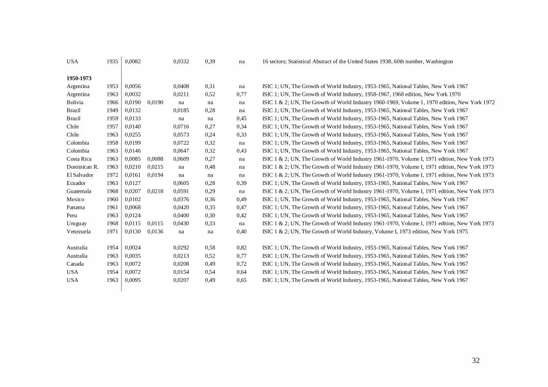
32

USA 1935 0,0082 0,0332 0,39 na 16 sectors; Statistical Abstract of the United States 1938, 60th number, Washington

1950-1973Argentina 1953 0,0056 0,0408 0,31 na ISIC 1; UN, The Growth of World Industry, 1953-1965, National Tables, New York 1967Argentina 1963 0,0032 0,0211 0,52 0,77 ISIC 1; UN, The Growth of World Industry, 1958-1967, 1968 edition, New York 1970Bolivia 1966 0,0190 0,0190 na na na ISIC 1 & 2; UN, The Growth of World Industry 1960-1969, Volume 1, 1970 edition, New York 1972Brazil 1949 0,0132 0,0185 0,28 na ISIC 1; UN, The Growth of World Industry, 1953-1965, National Tables, New York 1967Brazil 1959 0,0133 na na 0,45 ISIC 1; UN, The Growth of World Industry, 1953-1965, National Tables, New York 1967Chile 1957 0,0140 0,0716 0,27 0,34 ISIC 1; UN, The Growth of World Industry, 1953-1965, National Tables, New York 1967Chile 1963 0,0255 0,0573 0,24 0,33 ISIC 1; UN, The Growth of World Industry, 1953-1965, National Tables, New York 1967Colombia 1958 0,0199 0,0722 0,32 na ISIC 1; UN, The Growth of World Industry, 1953-1965, National Tables, New York 1967Colombia 1963 0,0146 0,0647 0,32 0,43 ISIC 1; UN, The Growth of World Industry, 1953-1965, National Tables, New York 1967Costa Rica 1963 0,0085 0,0088 0,0609 0,27 na ISIC 1 & 2; UN, The Growth of World Industry 1961-1970, Volume I, 1971 edition, New York 1973Dominican R. 1963 0,0210 0,0215 na 0,48 na ISIC 1 & 2; UN, The Growth of World Industry 1961-1970, Volume I, 1971 edition, New York 1973El Salvador 1972 0,0161 0,0194 na na na ISIC 1 & 2; UN, The Growth of World Industry 1961-1970, Volume I, 1971 edition, New York 1973Ecuador 1963 0,0127 0,0605 0,28 0,39 ISIC 1; UN, The Growth of World Industry, 1953-1965, National Tables, New York 1967Guatemala 1968 0,0207 0,0218 0,0591 0,29 na ISIC 1 & 2; UN, The Growth of World Industry 1961-1970, Volume I, 1971 edition, New York 1973Mexico 1960 0,0102 0,0376 0,36 0,49 ISIC 1; UN, The Growth of World Industry, 1953-1965, National Tables, New York 1967Panama 1961 0,0068 0,0420 0,35 0,47 ISIC 1; UN, The Growth of World Industry, 1953-1965, National Tables, New York 1967Peru 1963 0,0124 0,0400 0,30 0,42 ISIC 1; UN, The Growth of World Industry, 1953-1965, National Tables, New York 1967Uruguay 1968 0,0115 0,0115 0,0430 0,33 na ISIC 1 & 2; UN, The Growth of World Industry 1961-1970, Volume I, 1971 edition, New York 1973Venezuela 1971 0,0130 0,0136 na na 0,40 ISIC 1 & 2; UN, The Growth of World Industry, Volume I, 1973 edition, New York 1975

Australia 1954 0,0024 0,0292 0,58 0,82 ISIC 1; UN, The Growth of World Industry, 1953-1965, National Tables, New York 1967Australia 1963 0,0035 0,0213 0,52 0,77 ISIC 1; UN, The Growth of World Industry, 1953-1965, National Tables, New York 1967Canada 1963 0,0072 0,0208 0,49 0,72 ISIC 1; UN, The Growth of World Industry, 1953-1965, National Tables, New York 1967USA 1954 0,0072 0,0154 0,54 0,64 ISIC 1; UN, The Growth of World Industry, 1953-1965, National Tables, New York 1967USA 1963 0,0095 0,0207 0,49 0,65 ISIC 1; UN, The Growth of World Industry, 1953-1965, National Tables, New York 1967

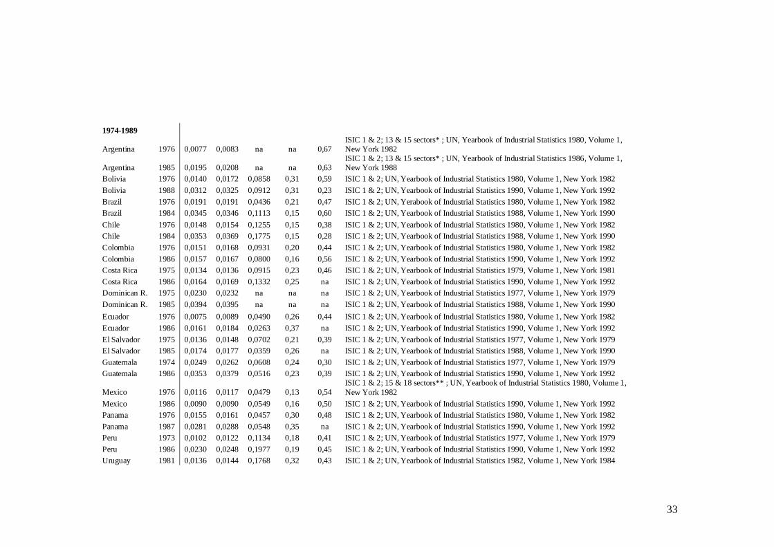
33

1974-1989

Argentina 1976 0,0077 0,0083 na na 0,67ISIC 1 & 2; 13 & 15 sectors* ; UN, Yearbook of Industrial Statistics 1980, Volume 1,New York 1982

Argentina 1985 0,0195 0,0208 na na 0,63ISIC 1 & 2; 13 & 15 sectors* ; UN, Yearbook of Industrial Statistics 1986, Volume 1,New York 1988

Bolivia 1976 0,0140 0,0172 0,0858 0,31 0,59 ISIC 1 & 2; UN, Yearbook of Industrial Statistics 1980, Volume 1, New York 1982Bolivia 1988 0,0312 0,0325 0,0912 0,31 0,23 ISIC 1 & 2; UN, Yearbook of Industrial Statistics 1990, Volume 1, New York 1992Brazil 1976 0,0191 0,0191 0,0436 0,21 0,47 ISIC 1 & 2; UN, Yerabook of Industrial Statistics 1980, Volume 1, New York 1982Brazil 1984 0,0345 0,0346 0,1113 0,15 0,60 ISIC 1 & 2; UN, Yearbook of Industrial Statistics 1988, Volume 1, New York 1990Chile 1976 0,0148 0,0154 0,1255 0,15 0,38 ISIC 1 & 2; UN, Yearbook of Industrial Statistics 1980, Volume 1, New York 1982Chile 1984 0,0353 0,0369 0,1775 0,15 0,28 ISIC 1 & 2; UN, Yearbook of Industrial Statistics 1988, Volume 1, New York 1990Colombia 1976 0,0151 0,0168 0,0931 0,20 0,44 ISIC 1 & 2; UN, Yearbook of Industrial Statistics 1980, Volume 1, New York 1982Colombia 1986 0,0157 0,0167 0,0800 0,16 0,56 ISIC 1 & 2; UN, Yearbook of Industrial Statistics 1990, Volume 1, New York 1992Costa Rica 1975 0,0134 0,0136 0,0915 0,23 0,46 ISIC 1 & 2; UN, Yearbook of Industrial Statistics 1979, Volume 1, New York 1981Costa Rica 1986 0,0164 0,0169 0,1332 0,25 na ISIC 1 & 2; UN, Yearbook of Industrial Statistics 1990, Volume 1, New York 1992Dominican R. 1975 0,0230 0,0232 na na na ISIC 1 & 2; UN, Yearbook of Industrial Statistics 1977, Volume 1, New York 1979Dominican R. 1985 0,0394 0,0395 na na na ISIC 1 & 2; UN, Yearbook of Industrial Statistics 1988, Volume 1, New York 1990Ecuador 1976 0,0075 0,0089 0,0490 0,26 0,44 ISIC 1 & 2; UN, Yearbook of Industrial Statistics 1980, Volume 1, New York 1982Ecuador 1986 0,0161 0,0184 0,0263 0,37 na ISIC 1 & 2; UN, Yearbook of Industrial Statistics 1990, Volume 1, New York 1992El Salvador 1975 0,0136 0,0148 0,0702 0,21 0,39 ISIC 1 & 2; UN, Yearbook of Industrial Statistics 1977, Volume 1, New York 1979El Salvador 1985 0,0174 0,0177 0,0359 0,26 na ISIC 1 & 2; UN, Yearbook of Industrial Statistics 1988, Volume 1, New York 1990Guatemala 1974 0,0249 0,0262 0,0608 0,24 0,30 ISIC 1 & 2; UN, Yearbook of Industrial Statistics 1977, Volume 1, New York 1979Guatemala 1986 0,0353 0,0379 0,0516 0,23 0,39 ISIC 1 & 2; UN, Yearbook of Industrial Statistics 1990, Volume 1, New York 1992

Mexico 1976 0,0116 0,0117 0,0479 0,13 0,54ISIC 1 & 2; 15 & 18 sectors** ; UN, Yearbook of Industrial Statistics 1980, Volume 1,New York 1982

Mexico 1986 0,0090 0,0090 0,0549 0,16 0,50 ISIC 1 & 2; UN, Yearbook of Industrial Statistics 1990, Volume 1, New York 1992Panama 1976 0,0155 0,0161 0,0457 0,30 0,48 ISIC 1 & 2; UN, Yearbook of Industrial Statistics 1980, Volume 1, New York 1982Panama 1987 0,0281 0,0288 0,0548 0,35 na ISIC 1 & 2; UN, Yearbook of Industrial Statistics 1990, Volume 1, New York 1992Peru 1973 0,0102 0,0122 0,1134 0,18 0,41 ISIC 1 & 2; UN, Yearbook of Industrial Statistics 1977, Volume 1, New York 1979Peru 1986 0,0230 0,0248 0,1977 0,19 0,45 ISIC 1 & 2; UN, Yearbook of Industrial Statistics 1990, Volume 1, New York 1992Uruguay 1981 0,0136 0,0144 0,1768 0,32 0,43 ISIC 1 & 2; UN, Yearbook of Industrial Statistics 1982, Volume 1, New York 1984

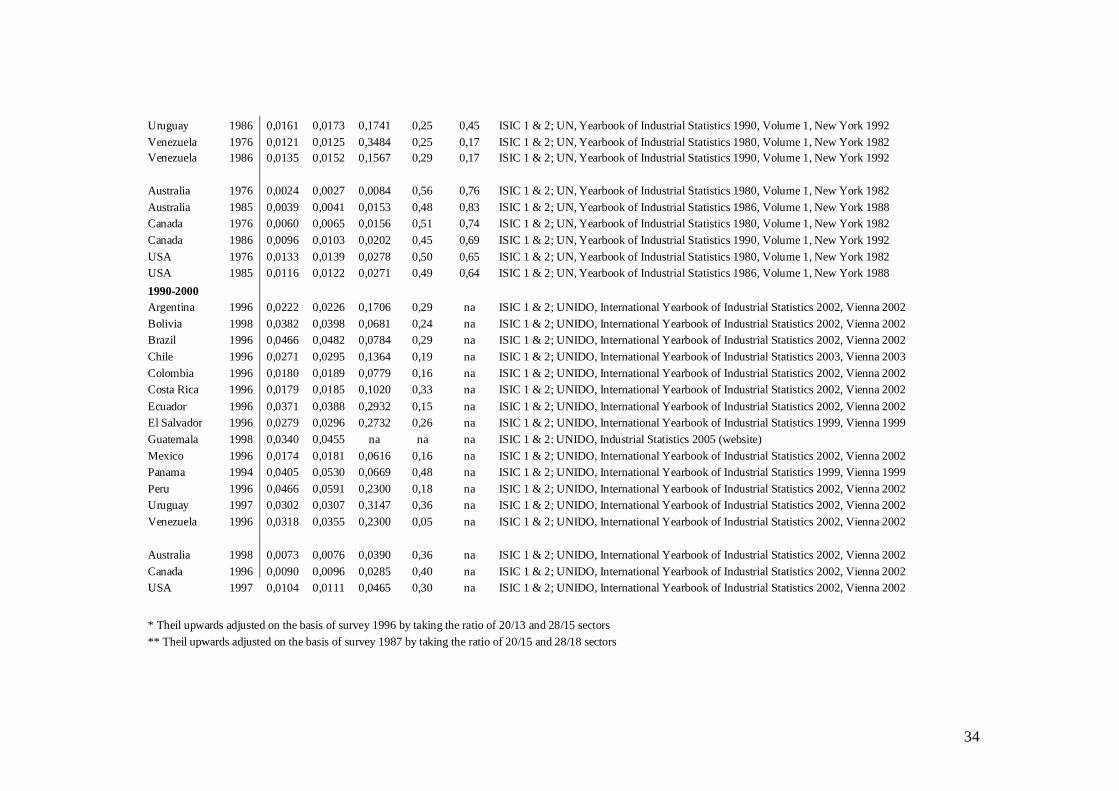
34

Uruguay 1986 0,0161 0,0173 0,1741 0,25 0,45 ISIC 1 & 2; UN, Yearbook of Industrial Statistics 1990, Volume 1, New York 1992Venezuela 1976 0,0121 0,0125 0,3484 0,25 0,17 ISIC 1 & 2; UN, Yearbook of Industrial Statistics 1980, Volume 1, New York 1982Venezuela 1986 0,0135 0,0152 0,1567 0,29 0,17 ISIC 1 & 2; UN, Yearbook of Industrial Statistics 1990, Volume 1, New York 1992

Australia 1976 0,0024 0,0027 0,0084 0,56 0,76 ISIC 1 & 2; UN, Yearbook of Industrial Statistics 1980, Volume 1, New York 1982Australia 1985 0,0039 0,0041 0,0153 0,48 0,83 ISIC 1 & 2; UN, Yearbook of Industrial Statistics 1986, Volume 1, New York 1988Canada 1976 0,0060 0,0065 0,0156 0,51 0,74 ISIC 1 & 2; UN, Yearbook of Industrial Statistics 1980, Volume 1, New York 1982Canada 1986 0,0096 0,0103 0,0202 0,45 0,69 ISIC 1 & 2; UN, Yearbook of Industrial Statistics 1990, Volume 1, New York 1992USA 1976 0,0133 0,0139 0,0278 0,50 0,65 ISIC 1 & 2; UN, Yearbook of Industrial Statistics 1980, Volume 1, New York 1982USA 1985 0,0116 0,0122 0,0271 0,49 0,64 ISIC 1 & 2; UN, Yearbook of Industrial Statistics 1986, Volume 1, New York 19881990-2000Argentina 1996 0,0222 0,0226 0,1706 0,29 na ISIC 1 & 2; UNIDO, International Yearbook of Industrial Statistics 2002, Vienna 2002Bolivia 1998 0,0382 0,0398 0,0681 0,24 na ISIC 1 & 2; UNIDO, International Yearbook of Industrial Statistics 2002, Vienna 2002Brazil 1996 0,0466 0,0482 0,0784 0,29 na ISIC 1 & 2; UNIDO, International Yearbook of Industrial Statistics 2002, Vienna 2002Chile 1996 0,0271 0,0295 0,1364 0,19 na ISIC 1 & 2; UNIDO, International Yearbook of Industrial Statistics 2003, Vienna 2003Colombia 1996 0,0180 0,0189 0,0779 0,16 na ISIC 1 & 2; UNIDO, International Yearbook of Industrial Statistics 2002, Vienna 2002Costa Rica 1996 0,0179 0,0185 0,1020 0,33 na ISIC 1 & 2; UNIDO, International Yearbook of Industrial Statistics 2002, Vienna 2002Ecuador 1996 0,0371 0,0388 0,2932 0,15 na ISIC 1 & 2; UNIDO, International Yearbook of Industrial Statistics 2002, Vienna 2002El Salvador 1996 0,0279 0,0296 0,2732 0,26 na ISIC 1 & 2; UNIDO, International Yearbook of Industrial Statistics 1999, Vienna 1999Guatemala 1998 0,0340 0,0455 na na na ISIC 1 & 2: UNIDO, Industrial Statistics 2005 (website)Mexico 1996 0,0174 0,0181 0,0616 0,16 na ISIC 1 & 2; UNIDO, International Yearbook of Industrial Statistics 2002, Vienna 2002Panama 1994 0,0405 0,0530 0,0669 0,48 na ISIC 1 & 2; UNIDO, International Yearbook of Industrial Statistics 1999, Vienna 1999Peru 1996 0,0466 0,0591 0,2300 0,18 na ISIC 1 & 2; UNIDO, International Yearbook of Industrial Statistics 2002, Vienna 2002Uruguay 1997 0,0302 0,0307 0,3147 0,36 na ISIC 1 & 2; UNIDO, International Yearbook of Industrial Statistics 2002, Vienna 2002Venezuela 1996 0,0318 0,0355 0,2300 0,05 na ISIC 1 & 2; UNIDO, International Yearbook of Industrial Statistics 2002, Vienna 2002

Australia 1998 0,0073 0,0076 0,0390 0,36 na ISIC 1 & 2; UNIDO, International Yearbook of Industrial Statistics 2002, Vienna 2002Canada 1996 0,0090 0,0096 0,0285 0,40 na ISIC 1 & 2; UNIDO, International Yearbook of Industrial Statistics 2002, Vienna 2002USA 1997 0,0104 0,0111 0,0465 0,30 na ISIC 1 & 2; UNIDO, International Yearbook of Industrial Statistics 2002, Vienna 2002

* Theil upwards adjusted on the basis of survey 1996 by taking the ratio of 20/13 and 28/15 sectors** Theil upwards adjusted on the basis of survey 1987 by taking the ratio of 20/15 and 28/18 sectors

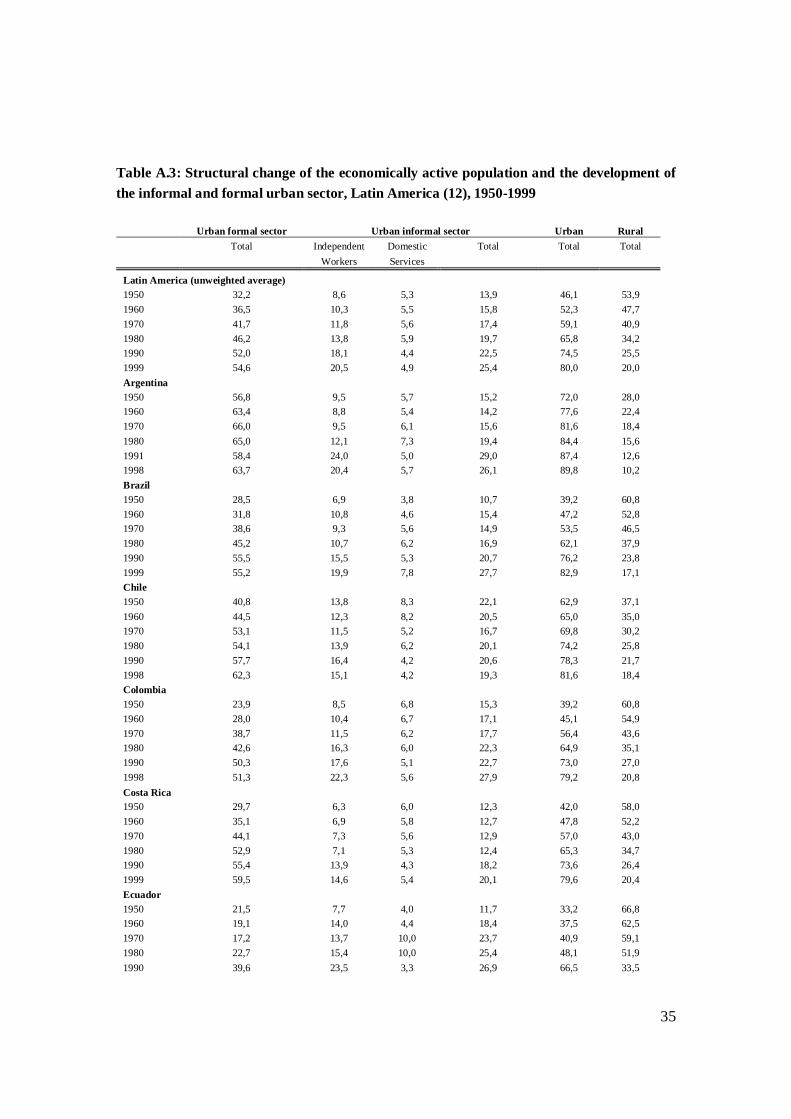
35

Table A.3: Structural change of the economically active population and the development ofthe informal and formal urban sector, Latin America (12), 1950-1999

Urban formal sector Urban informal sector Urban RuralTotal Independent Domestic Total Total Total

Workers Services

Latin America (unweighted average)1950 32,2 8,6 5,3 13,9 46,1 53,91960 36,5 10,3 5,5 15,8 52,3 47,71970 41,7 11,8 5,6 17,4 59,1 40,91980 46,2 13,8 5,9 19,7 65,8 34,21990 52,0 18,1 4,4 22,5 74,5 25,51999 54,6 20,5 4,9 25,4 80,0 20,0Argentina1950 56,8 9,5 5,7 15,2 72,0 28,01960 63,4 8,8 5,4 14,2 77,6 22,41970 66,0 9,5 6,1 15,6 81,6 18,41980 65,0 12,1 7,3 19,4 84,4 15,61991 58,4 24,0 5,0 29,0 87,4 12,61998 63,7 20,4 5,7 26,1 89,8 10,2Brazil1950 28,5 6,9 3,8 10,7 39,2 60,81960 31,8 10,8 4,6 15,4 47,2 52,81970 38,6 9,3 5,6 14,9 53,5 46,51980 45,2 10,7 6,2 16,9 62,1 37,91990 55,5 15,5 5,3 20,7 76,2 23,81999 55,2 19,9 7,8 27,7 82,9 17,1Chile1950 40,8 13,8 8,3 22,1 62,9 37,11960 44,5 12,3 8,2 20,5 65,0 35,01970 53,1 11,5 5,2 16,7 69,8 30,21980 54,1 13,9 6,2 20,1 74,2 25,81990 57,7 16,4 4,2 20,6 78,3 21,71998 62,3 15,1 4,2 19,3 81,6 18,4Colombia1950 23,9 8,5 6,8 15,3 39,2 60,81960 28,0 10,4 6,7 17,1 45,1 54,91970 38,7 11,5 6,2 17,7 56,4 43,61980 42,6 16,3 6,0 22,3 64,9 35,11990 50,3 17,6 5,1 22,7 73,0 27,01998 51,3 22,3 5,6 27,9 79,2 20,8Costa Rica1950 29,7 6,3 6,0 12,3 42,0 58,01960 35,1 6,9 5,8 12,7 47,8 52,21970 44,1 7,3 5,6 12,9 57,0 43,01980 52,9 7,1 5,3 12,4 65,3 34,71990 55,4 13,9 4,3 18,2 73,6 26,41999 59,5 14,6 5,4 20,1 79,6 20,4Ecuador1950 21,5 7,7 4,0 11,7 33,2 66,81960 19,1 14,0 4,4 18,4 37,5 62,51970 17,2 13,7 10,0 23,7 40,9 59,11980 22,7 15,4 10,0 25,4 48,1 51,91990 39,6 23,5 3,3 26,9 66,5 33,5

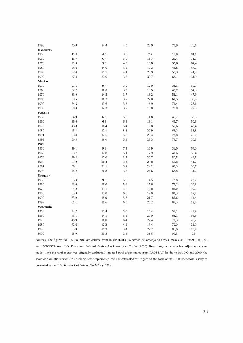
36

1998 45,0 24,4 4,5 28,9 73,9 26,1Honduras1950 11,4 4,5 3,0 7,5 18,9 81,11960 16,7 6,7 5,0 11,7 28,4 71,61970 21,8 9,8 4,0 13,8 35,6 64,41980 25,6 14,0 3,2 17,2 42,8 57,21990 32,4 21,7 4,1 25,9 58,3 41,71999 37,4 27,0 3,7 30,7 68,1 31,9Mexico1950 21,6 9,7 3,2 12,9 34,5 65,51960 32,2 10,0 3,5 13,5 45,7 54,31970 33,9 14,5 3,7 18,2 52,1 47,91980 39,5 18,3 3,7 22,0 61,5 38,51990 54,5 13,6 3,3 16,9 71,4 28,61999 60,0 14,3 3,7 18,0 78,0 22,0Panama1950 34,9 6,3 5,5 11,8 46,7 53,31960 36,6 6,8 6,3 13,1 49,7 50,31970 43,8 10,4 5,4 15,8 59,6 40,41980 45,3 12,1 8,8 20,9 66,2 33,81991 53,4 14,6 5,8 20,4 73,8 26,21999 56,4 18,0 5,3 23,3 79,7 20,3Peru1950 19,1 9,8 7,1 16,9 36,0 64,01960 23,7 12,8 5,1 17,9 41,6 58,41970 29,8 17,0 3,7 20,7 50,5 49,51980 35,0 20,4 3,4 23,8 58,8 41,21991 39,1 21,1 3,1 24,2 63,3 36,71998 44,2 20,8 3,8 24,6 68,8 31,2Uruguay1950 63,3 9,0 5,5 14,5 77,8 22,21960 63,6 10,0 5,6 15,6 79,2 20,81970 64,2 11,1 5,7 16,8 81,0 19,01980 63,3 13,0 6,0 19,0 82,3 17,71990 63,9 15,9 5,8 21,7 85,6 14,41999 61,1 19,6 6,5 26,2 87,3 12,7Venezuela1950 34,7 11,4 5,0 16,4 51,1 48,91960 43,1 14,1 5,9 20,0 63,1 36,91970 48,9 16,0 6,4 22,4 71,3 28,71980 62,6 12,2 4,2 16,4 79,0 21,01990 63,9 19,3 3,4 22,7 86,6 13,41999 58,9 29,3 2,3 31,6 90,5 9,5

Sources: The figures for 1950 to 1980 are derived from ILO/PREALC, Mercado de Trabajo en Cifras. 1950-1980 (1982); For 1990

and 1998/1999 from ILO, Panorama Laboral de America Latina y el Caribe (2000). Regarding the latter a few adjustments were

made: since the rural sector was originally excluded I imputed rural-urban shares from FAOSTAT for the years 1990 and 2000; the

share of domestic servants in Colombia was suspiciously low, I re-estimated this figure on the basis of the 1990 Household survey as

presented in the ILO, Yearbook of Labour Statistics (1991).