A “vertically Lagrangian” finite-volume dynam- ical core for global models

Submitted to Monthly Weather Review

Shian-Jiann Lin Data Assimilation Office

NASA Goddard Space Flight Center Greenbelt, MD 20771

by

Corresponding author address: Dr. Shian-Jiann Lin, code 910.3, NASA Goddard Space Flight Center, Greenbelt, MD 20771. E-mail: Shian-Jiann.Lin-l@nasa.gov

1

https://ntrs.nasa.gov/search.jsp?R=20030052220 2018-05-30T18:28:45+00:00Z

Abstract

A finite-volume dynamical core with a terrain-following Lagrangian control-volume

discretization is described. The vertically Lagrangian discretization reduces the dimen-

sionality of the physical problem from three to two with the resulting dynamical system

closely resembling that of the shallow water dynamical system. The 2D horizontal-to-

Lagrangian-surface transport and dynamical processes are then discretized using the

genuinely conservative flux-form semi-Lagrangian algorithm. Time marching is split-

explicit, with large-time-step for scalar transport, and small fractional time step for

the Lagrangian dynamics, which permits the accurate propagation of fast waves. A

mass, momentum, and total energy conserving algorithm is developed for mapping the

state variables periodically from the floating Lagrangian control-volume to an Eulerian

terrain-following coordinate for dealing with “physical parameterizations” and to pre-

vent severe distortion of the Lagrangian surfaces. Deterministic baroclinic wave growth

tests and long-term integrations using the Held-Suarez forcing are presented. Impact

of the monotonicity constraint is discussed.

2

1. Introduction

This paper describes the finite-volume dynamical core for global models that was devel-

o'ped at the NASA Goddard Space Flight Center. We review in section 1.1 the motivation

and development history of the finite-volume dynamical core and the associated algorithms.

Readers not interested in this history can jump to section 1.2 where the governing equations

fix the atmosphere under the hydrostatic approximation are written using a general vertical

coordinate. Upon the introduction of the Lagrangian control-volume vertical discretization,

all prognostic equations are reduced to 2D, in the sense that they are vertically decoupled.

The discretization of the 2D horizontal transport process is described in section 2. The

complete dynamical system with the La,grangian control-volume vertical discretization is de-

scribed in section 3. A mass, momentum, and total energy conserving mapping algorithm

is described in section 4. We present in section 5, the deterministic baroclinic wave growth

tests and long term integrations using the Held-Suarez forcing (Held and Suarez 1994).

Concluding remarks are given in section 6.

l . 1 A review of the finite-volume algorithm developments at NASA Goddard

Space Flight Center

The developments and applications of the finite-volume algorithms for global modeling at

NASA Goddard Space Flight Center (GSFC) started in the late 80s and early 90s with focus

o'n the transport process of chemistry constituents (e.g., Rood 1987; Allen et al. 1991 and

1996) and water vapor (Lin et ai. 1994). These algorithms were derived and evolved from the

modern 1D finite-volume algorithms pioneered by van Leer (1977) and Colella and Woodward

(1984), which were originally designed for resolving sharp gradients and discontinuities in

astrophysics and aerospace engineering applications. Many of those algorithms emphasize

sound-wave dominant flows, which carry no meteorological significance on the global scale.

The challenge to us was to develop computationally competitive and physically based

algorithms suitable for global modeling of the geophysical flows. There exists rich body of

3

literature on high performance finite-volume schemes designed for entirely different disci-

plines (e.g., Woodward and Colella 1984). The large-scale atmospheric flow is highly strati-

fied in the direction of gravitation, and as an excellent approximation, hydrostatic. As such,

the standard “Riemann solver” for non-hydrostatic flows (e.g., Carpenter et al. 1991) would

not be efficient nor applicable. Furthermore, the directional splitting needed for applying

the above-mentioned 1D algorithms would produce unacceptably large errors near the poles

where the splitting errors are greatly amplified by the convergence of the meridians.

A milestone was achieved in early 1994l with the development of the multi-dimensional

“Flux-Form Semi-Lagrangian Transport” scheme (FFSL, Lin and Rood 1996; referred to

a,s LR96 hereafter). Building on the existing 1D finite-volume algorithms (e.g., PPM), the

E‘FSL algorithm extended those schemes to multidimensions and thereby eliminated the need

fix directional splitting. Equally important, the so-called “Pole-Courant number problem” is

solved, via the physical consideration of the contribution to fluxes from upstream volumes

ass far away as the Courant number indicated. The resulting multi-dimensional scheme is

oscillation free (with the optional monotonicity constraint), mass conserving, and stable for

Courant number greater than one, which made the scheme competitive for the intended ap-

plication on the sphere. The FFSL algorithm has since been adopted in several atmospheric

chemistry transport applications (e.g., Rotman et al. 2001).

Another milestone towards the goal of building the finite-volume dynamical core was

reached with the adaptation of the FFSL algorithm to the shallow water dynamical frame-

work (Lin and Rood 1997; referred to as LR97 hereafter). A “reversed engineering approach”

was devised in LR97 to achieve the design goal of consistent transport of the mass (layer

thickness), the absolute vorticity, and hence, the potential vorticity. The reversed engi-

neering approach is a two-grid (C and D grids) two-step procedure design to achieve the

consistent transport of absolute vorticity and mass without the computational expense of

using explicitly the Z grid (Randall 1994), which requires an elliptic solver. The time dis-

‘The multi-dimensional Flux-Form Transport Algorithm was first presented in 1994 at the 4th Workshop on the Solutions of Partial Differential Equations on the Sphere and later published in 1996.

-

4

cretization for treating the gravity waves on both grids is the explicit “forward-backward”

scheme, which is conditionally stable with the forward-in-time nature of the FFSL transport

a,lgorithm. The allowable size of the time step, for example, for a T42 like resolution (about

2.8’) is 600 seconds, which is about half of what can be used by the semi-implicit Eulerian

spectral model. This not-so-small time step made the fully explicit shallow water algorithm

computationally competitive with the traditional spectral and finite difference methods (e.g.,

Pirakawa and Lamb 1981).

The final piece needed for the completion of the finite-volume dynamical core was devel-

oped after the discovery of a very simple finite-volume integration method for computing the

pressure gradient in general terrain-following coordinates (Lin 1997 and 1998; referred to as

L97 and L98 hereafter). It is well known that the standard mathematical transformation of

the pressure gradient term in terrain-following coordinates results in two large-in-magnitude

terms with opposite sign. A straightforward application of numerical techniques (e.g., center

d5fferencing) to these two terms would typically produce large errors. The finite-volume in-

tegration scheme of L97 avoids the mathematical transformation by integrating around the

arbitrarily shaped finite-volume to accurately determine the pressure gradient forcing that

maintains physical consistency for the finite volume under consideration.

The finite-volume dynamical core developed in L97 utilized a sigma vertical coordinate,

which requires a 3D transport algorithm. Applying the methodology of LR96, a fully 3D

E’FSL algorithm would require 6 permutations of 1D operators, instead of 2 as in 2D. To

reduce computational cost, a simplification was made in L97, with some loss in accuracy,

to reduce the operator permutations from 6 to 3, and even down to 2 (i.e., no cross terms

associated with vertical transport, as was done in Eq. 4.2 of LR96). This compromise was

a, concern until the introduction of the Lagrangian control-volume vertical discretization

(Lin and Rood 1998 and Lin and Rood 1999; fully described in section 3). A 3D transport

algorithm is no longer required as the dimensionality of the physical problem is essentially

reduced from three to two, as viewed from the Lagrangian control-volume perspective.

5

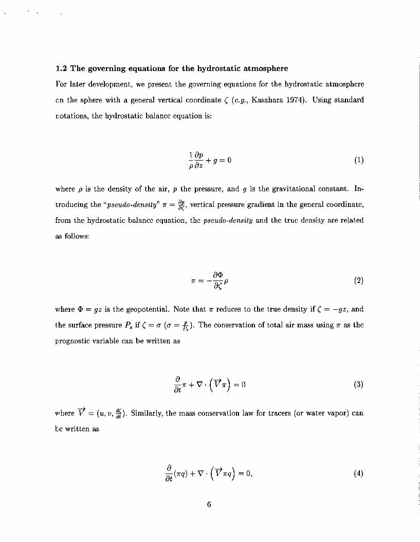
l .2 The governing equations for the hydrostatic atmosphere

For later development, we present the governing equations for the hydrostatic atmosphere

cln the sphere with a general vertical coordinate c (e.g., Kasahara 1974). Using standard

notations, the hydrostatic balance equakion is:

where p is the density of the air, p the pressure, and g is the gravitational constant. In-

troducing the “pseudo-density” 7r = $, vertical pressure gradient in the general coordinate,

from the hydrostatic balance equation, the pseudo-density and the true density are related

as follows:

where @ = gz is the geopotential. Note that 7r reduces to the true density if = -gz, and

the surface pressure P, if c = o (o = E). The conservation of total air mass using 7r as the

prognostic variable can be written as

a at -7r+v. (V7r) = o (3)

where ? = (u, v, s). Similarly, the mass conservation law for tracers (or water vapor) can

be written as

a at -(7rq) + v (Q.9) = 0, (4)

6

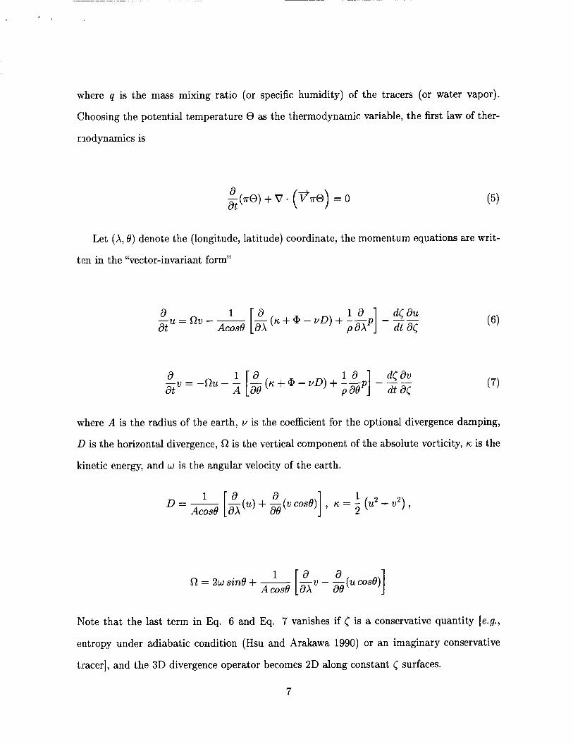
where q is the mass mixing ratio (or specific humidity) of the tracers (or water vapor).

Choosing the potential temperature 0 as the thermodynamic variable, the first law of ther-

modynamics is

(5) a at -(TO) + v - (A@) = 0

Let (A, 6) denote the (longitude, latitude) coordinate, the momentum equations are writ-

ten in the "vector-invariant form"

d< av P ] dt a<

a ( K + @ - vD) + - - p - -- (7)

where A is the radius of the earth, Y is the coefficient for the optional divergence damping,

L ) is the horizontal divergence, R is the vertical component of the absolute vorticity, K is the

kinetic energy, and w is the angular velocity of the earth.

1

R = 2w sin6 +

Note that the last term in Eq. 6 and Eq. 7 vanishes if ( is a conservative quantity [e.g.,

entropy under adiabatic condition (Hsu and Arakawa 1990) or an imaginary conservative

tracer], and the 3D divergence operator becomes 2D along constant < surfaces.

7

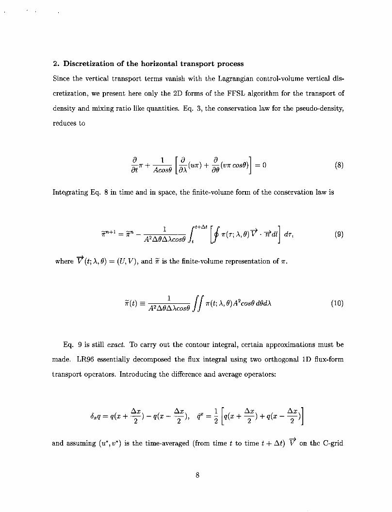
41. Discretization of the horizontal transport process

Since the vertical transport terms vanish with the Lagrangian control-volume vertical dis-

cretization, we present here only the 2D forms of the FFSL algorithm for the transport of

dlensity and mixing ratio like quantities. Eq. 3, the conservation law for the pseudo-density,

reduces to

1 a ae

a + - case) = o

Integrating Eq. 8 in time and in space, the finite-volume form of the conservation law is

t+At zn+l = +yn - 1 / [/ T ( T ; A, e)? - $dl] dT,

A2AOAAcosB

.where ?(t; A, 0 ) = (U, V ) , and F is the finite-volume representation of T.

c c // T ( t ; A, 8)A2cosB d0dA 1 %(t) =

A2A 0 A Xcose

(9)

Eq. 9 is still exact. To carry out the contour integral, certain approximations must be

made. LR96 essentially decomposed the flux integral using two orthogonal 1D flux-form

transport operators. Introducing the difference and average operators:

Ax Ax &q = q(x + -1 - -

2

and assuming (u*, v*) is the time-averaged (from time t to time t + At) 9 on the C-grid

8

(e.g., Fig. 1 in LR96), the 1-D flux-form transport operator F i n the A-direction is

x(u*, At; T ) = d J d r = u*T*(u*, At, Z)

1 t+At n*(u*,At;?) x rdr

where x is the time-accumulated (from t to t+At) mass flux across the cell wall, and T*

can be interpreted as a time-mean (from time t to time t + At) pseudo-density value of

all material that passed through the cell edge. Note that the time integration in Eq. 13

is to be carried out along the backward-in-time trajectory of the cell edge position from

t = t + At back to time t. The very essence of the 1D finite-volume algorithm is to construct,

based on the given initial cell-mean values of F, an approximated subgrid distribution of the

true T field, to enable an analytic integration of Eq. 13. Assuming there is no error in

obtaining the time-mean wind (u’), the only error produced by the 1D transport scheme

would be solely due to the approximation to the continuous distribution of T using the

subgrid distribution. From this perspective, it can be said that the 1D finite-volume transport

algorithm combined the space-time discretization in the approximation of the time-mean cell-

edge value T’. The physically correct way of approximating the integral (Eq. 13) must be

“upwind”, in the sense that it is integrahed along the backward trajectory of the cell edges.

A center difference approximation to Eq. 13 would be physically incorrect, and consequently

numerically unstable unless artificial numerical diffusion is added.

9

Central to the accuracy and computational efficiency of the finite-volume algorithms

is the degrees of freedom that describe the subgrid distribution. The first order upwind

scheme has zero degree of freedom within the volume as it is assumed that the subgrid

distribution is piecewise constant having the same value everywhere within the cell as the

given volume-mean. The second order finite-volume scheme assumes a piece-wise linear

subgrid distribution, which allows one degree of freedom for the specification of the “slope”

(or equivalently, the “mismatch” as defined by Lin et al. 1994). The Piecewise Parabolic

Method (PPM) has two degrees of freedom in the construction of the second order polynomial

within the volume, and as a result, the accuracy is significantly enhanced. The PPM strikes

a, good balance between computational efficiency and accuracy. Therefore, it is the basic

1D scheme we chose. To further improve its accuracy, a modified PPM is described in the

a,ppendix.

While the PPM possesses all the desirable attributes (mass conserving, monotonicity pre-

serving, and high-order accuracy) in lD, a solution must be found to avoid the directional

splitting in modeling the dynamics and transport processes of the Earth’s atmosphere. The

first step towards reducing the splitting error is to apply the two orthogonal 1D flux-form op-

erators in a symmetric way. After the directional symmetry is achieved, the “inner operators”

are then replaced with corresponding advective-form operators. A consistent advective-form

operator (f) in the A-direction can be derived from its flux-form counterpart ( F ) as follows.

f(u*, At, E ) = F(u*, At, E ) - E F(u*, At, E E 1) = F(u*, At, %) + % C& (14)

At ~ X U *

c‘ef = AAAcos9

where C&, is a dimensionless number indicating the degree of the flow deformation in the

10

>,-direction. The above derivation of f is different from LR96's approach, which adopted the

traditional 1D advective-form semi-Lagrangian scheme. The advantage of using Eq. 14 is

that computations of winds at cell centers are avoided.

Analogously, 1D flux-form transport operator G in the latitudinal (e) direction is derived

a,s follows.

a.nd likewise the advective-form operator

g(v*, At, ?) = G(v*, At, F) + F CLf

where

Introducing the following short hand notations:

the 2D transport algorithm on the sphere can then be written as

11

;jjn+l - - T -n + F [u*, At, ze] + G [v*, At, ZA]

IJsing explicitly the mass fluxes (x, Y ) , Eq. 21 is rewritten as

1 { h~ [x:(u*, At; F e ) ] + -60 [cos8 Y(v*, At; ZA)] At zn+l = z n AcosO AA AO

where Y , the mass flux in the meridional direction, is defined in a similar fashion as x. It can be verified that in the special case of constant density flow, ;ii = constant, the above

equation degenerates to the discrete representation of the incompressibility condition of the

wind field (u*, v*)

1 ' 1 AA A 0 ---bAU* + -60 (v*cosO) = 0

The fulfillment of the above incompressibility condition for constant density flows is

crucial to the accuracy of the 2D flux-form formulation. For transport of mixing ratio like

quantities (3 the mass fluxes (x, Y ) as defined previously should be used as follows.

Note that the above form of the tracer transport equation consistently degenerates to Eq

22 if = constant, which is another important condition for a flux-form transport algorithm

tlo be able to avoid generation of of artificial gradients and to maintain mass conservation.

12

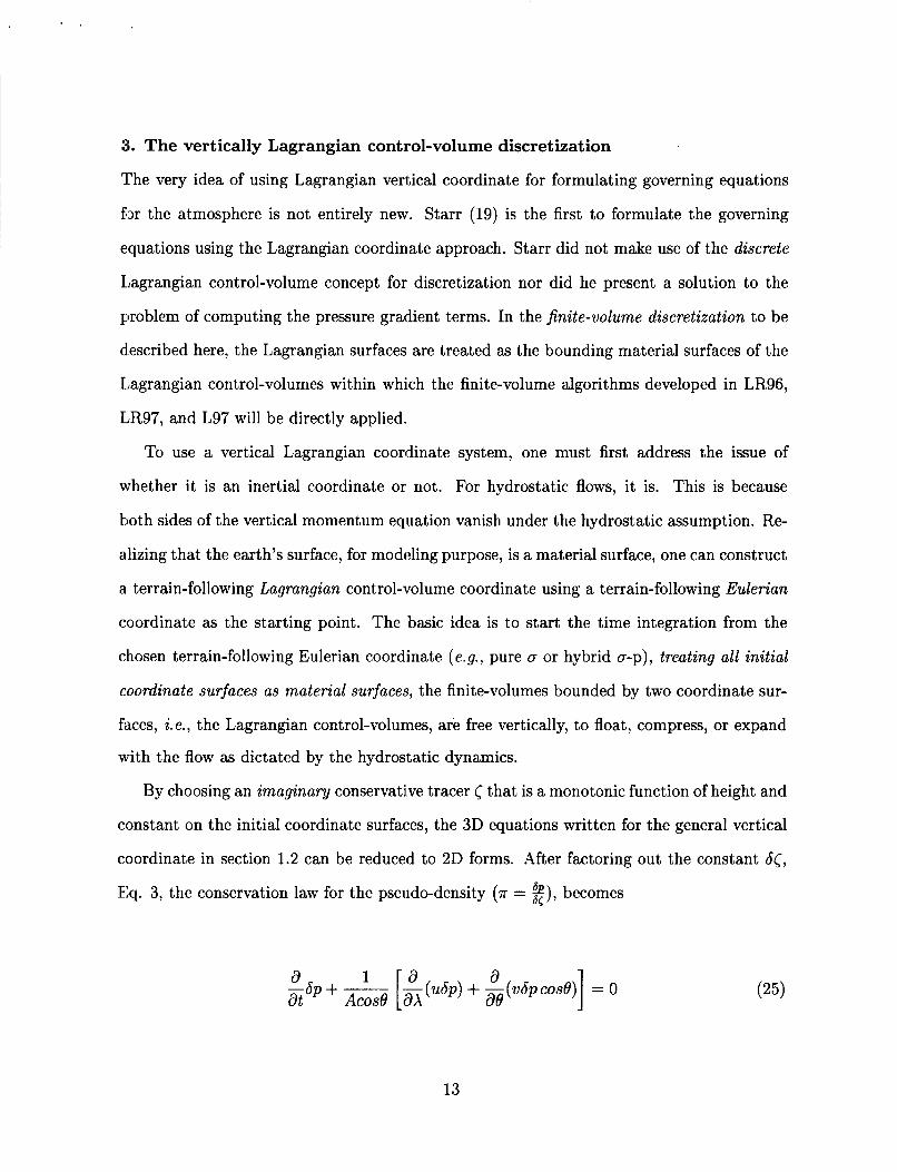
31. The vertically Lagrangian control-volume discretization

The very idea of using Lagrangian vertical coordinate for formulating governing equations

fix the atmosphere is not entirely new. Starr (19) is the first to formulate the governing

equations using the Lagrangian coordinate approach. Starr did not make use of the discrete

Lagrangian control-volume concept for discretization nor did he present a solution to the

problem of computing the pressure gradient terms. In the finite-volume discretization to be

d.escribed here, the Lagrangian surfaces are treated as the bounding material surfaces of the

Lagrangian control-volumes within which the finite-volume algorithms developed in LR96,

11R97, and L97 will be directly applied.

To use a vertical Lagrangian coordinate system, one must first address the issue of

whether it is an inertial coordinate or not. For hydrostatic flows, it is. This is because

both sides of the vertical momentum equation vanish under the hydrostatic assumption. Re-

alizing that the earth’s surface, for modeling purpose, is a material surface, one can construct

a, terrain-following Lagrangian control-volume coordinate using a terrain-following Eulerian

coordinate as the starting point. The basic idea is to start the time integration from the

chosen terrain-following Eulerian coordinate (e.g., pure a or hybrid a-p), treating all initial

coordinate surfaces as material surfaces, the finite-volumes bounded by two coordinate sur-

faces, i. e., the Lagrangian control-volumes, are free vertically, to float, compress, or expand

with the flow as dictated by the hydrostatic dynamics.

By choosing an imagina y conservative tracer that is a monotonic function of height and

constant on the initial coordinate surfaces, the 3D equations written for the general vertical

coordinate in section 1.2 can be reduced to 2D forms. After factoring out the constant c5[,

E:q. 3, the conservation law for the pseudo-density (T = $), becomes

1 --sp + - [--(&) + -((V-spcosO) = 0 a 1 a a at A C O ~ i9X a0

13

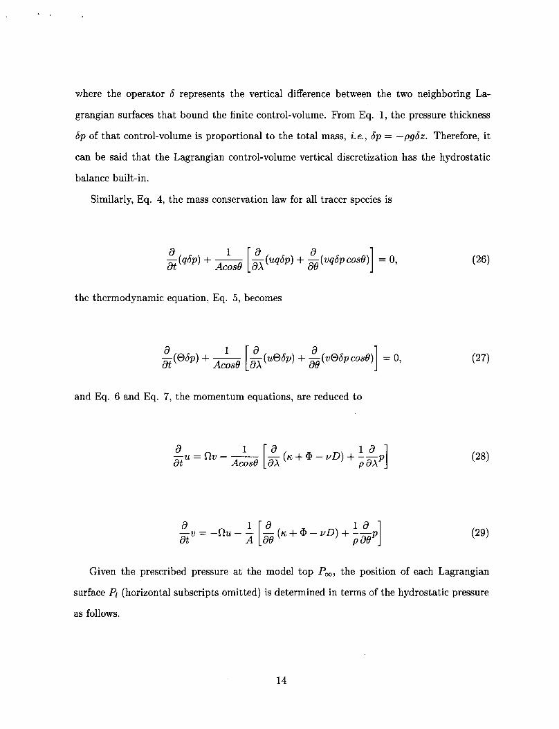
where the operator 6 represents the vertical difference between the two neighboring La-

grangian surfaces that bound the finite control-volume. From Eq. 1, the pressure thickness

6 p of that control-volume is proportional to the total mass, ie., 6p = -pgGz. Therefore, it

can be said that the Lagrangian control-volume vertical discretization has the hydrostatic

balance built-in.

Similarly, Eq. 4, the mass conservation law for all tracer species is

the thermodynamic equation, Eq. 5 , becomes

1 a 1 a a - (osp) + ~ [ -- (uo6p) + - (vo6p case) = 0, at Acose ax ae

a,nd Eq. 6 and Eq. 7, the momentum equations, are reduced to

a

P

a ( K + @ - vD) + --p (29)

Given the prescribed pressure at the model top Pm, the position of each Lagrangian

surface Pl (horizontal subscripts omitted) is determined in terms of the hydrostatic pressure

as follows.

14

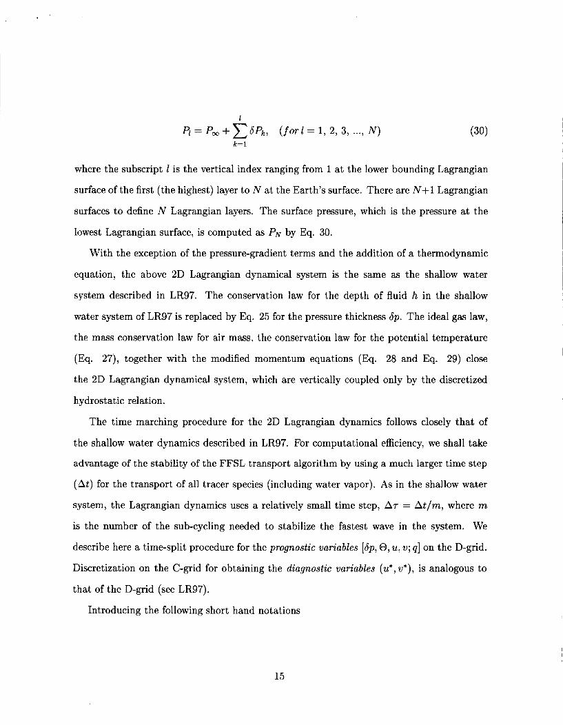
where the subscript 1 is the vertical index ranging from 1 at the lower bounding Lagrangian

surface of the first (the highest) layer to N at the Earth’s surface. There are N+l Lagrangian

surfaces to define N Lagrangian layers. The surface pressure, which is the pressure at the

lowest Lagrangian surface, is computed as PN by Eq. 30.

With the exception of the pressure-gradient terms and the addition of a thermodynamic

equation, the above 2D Lagrangian dynamical system is the same as the shallow water

system described in LR97. The conservation law for the depth of fluid h in the shallow

water system of LR97 is replaced by Eq. 25 for the pressure thickness Sp. The ideal gas law,

the mass conservation law for air mass, the conservation law for the potential temperature

(Eq. 27), together with the modified momentum equations (Eq. 28 and Eq. 29) close

the 2D Lagrangian dynamical system, which are vertically coupled only by the discretized

hydrostatic relation.

The time marching procedure for the 2D Lagrangian dynamics follows closely that of

the shallow water dynamics described in LR97. For computational efficiency, we shall take

advantage of the stability of the FFSL transport algorithm by using a much larger time step

( A t ) for the transport of all tracer species (including water vapor). As in the shallow water

system, the Lagrangian dynamics uses a relatively small time step, AT = At/rn, where rn

is the number of the sub-cycling needed to stabilize the fastest wave in the system. We

describe here a time-split procedure for the prognostic variables [bp, 0, u, v; q] on the D-grid.

Iliscretization on the C-grid for obtaining the diagnostic variables (u*, v*), is analogous to

that of the D-grid (see LR97).

Introducing the following short hand notations

15

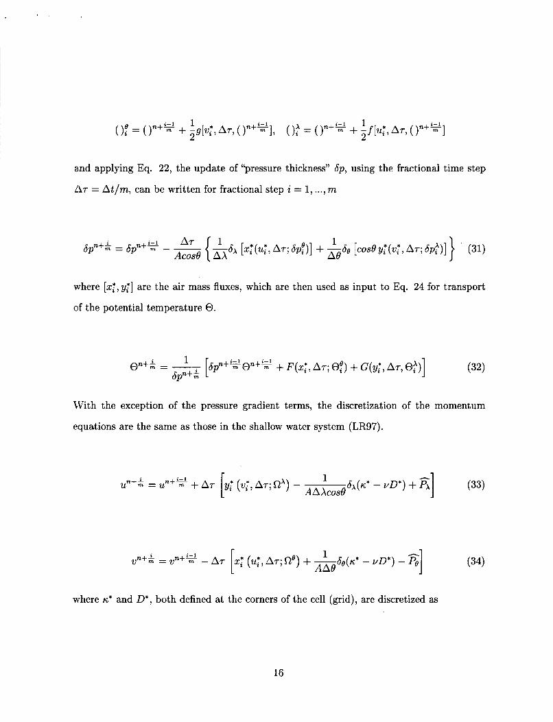
aad applying Eq. 22, the update of “pressure thickness” Sp, using the fractional time step

AT = At/m, can be written for fractional step i = 1, ..., m

where [~r,y:] are the air mass fluxes, which are then used as input to Eq. 24 for transport

of the potential temperature 0.

With the exception of the pressure gradient terms, the discretization of the momentum

equations are the same as those in the shallow water system (LR97).

&(K* - vD*) + A] (33) 1

AAAcosO (u t , AT; Cf’) - Un+$ = U n + g

-1 1 AAO

X: (u;, AT; ne) + - S ~ ( K * - YD*) - Po i - 1 vn+$ = ,p+T - (34)

where K* and D*, both defined at the corners of the cell (grid), are discretized as

16

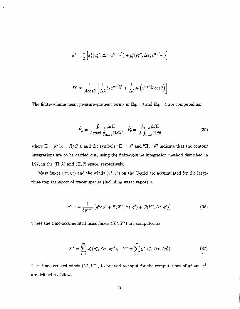
The finite-volume mean pressure-gradient terms in Eq. 33 and Eq. 34 are computed as:

where n = p K ( K = R/C,), and the symbols “II + A’’ and “II+ 0” indicate that the contour

integrations are to be carried out, using the finite-volume integration method described in

L,97, in the (II, A) and (ll, 0) space, respectively.

Mass fluxes (z*, y*) and the winds (u*, v*) on the C-grid are accumulated for the large-

time-step transport of tracer species (including water vapor) q.

f + l = - [qn6pn + F ( X * , At, 4’) + G(Y*, At, q’)] 6pn+l

where the time-accumulated mass fluxes ( X * , Y*) are computed as

m m

i= l i=l

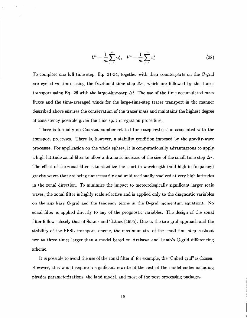
The time-averaged winds (V*, V*) , to be used as input for the computations of qA and q8,

are defined as follows.

17

. .

i

To complete one full time step, Eq. 31-34, together with their counterparts on the C-grid

axe cycled m times using the fractional time step Ar, which are followed by the tracer

transport using Eq. 26 with the large-time-step At. The use of the time accumulated mass

fluxes and the time-averaged winds for the large-time-step tracer transport in the manner

described above ensures the conservation of the tracer mass and maintains the highest degree

of consistency possible given the time split integration procedure.

There is formally no Courant number related time step restriction associated with the

transport processes. There is, however, a stability condition imposed by the gravity-wave

processes. For application on the whole sphere, it is computationally advantageous to apply

a high-latitude zonal filter to allow a dramatic increase of the size of the small time step AT.

The effect of the zonal filter is to stabilize the short-in-wavelength (and high-in-frequency)

gravity waves that are being unnecessarily and unidirectionally resolved at very high latitudes

in the zonal direction. To minimize the impact to meteorologically significant larger scale

waves, the zonal filter is highly scale selective and is applied only to the diagnostic variables

on the auxiliary C-grid and the tendency terms in the D-grid momentum equations. No

zonal filter is applied directly to any of the prognostic variables. The design of the zonal

filter follows closely that of Suarez and Takacs (1995). Due to the two-grid approach and the

stability of the FFSL transport scheme, the maximum size of the small-time-step is about

two to three times larger than a model based on Arakawa and Lamb’s C-grid differencing

scheme.

It is possible to avoid the use of the zonal filter if, for example, the “Cubed grid” is chosen.

However, this would require a significant rewrite of the rest of the model codes including

physics parameterizations, the land model, and most of the post processing packages.

18

The size of the small-time-step for the Lagrangian dynamics is only a function of the

hlorizontal resolution. Applying the zonal filter, for the 2-degree horizontal resolution, a

small-time-step size of 450 seconds can be used for the Lagrangian dynamics. From the

lisrge-time-step transport perspective, the small-time-step integration of the 2D Lagrangian

dlynamics can be regarded as a very accurate iterative solver, with rn iterations, for comput-

i:ng the time mean winds and the mass fluxes, analogous in functionality to a semi-implicit

algorithm’s elliptic solver (e.g., Ringler et al. 2000). Besides accuracy, the merit of “explicit”

versus “semi-implicit” algorithm ultimately depends on the computational efficiency of each

a,pproach. In light of the advantage of the explicit algorithm in parallelization, we do not

regard the explicit algorithm for the Lagrangian dynamics as an impedance to computational

efficiency.

4:. A mass, momentum, and total energy conserving mapping algorithm

The Lagrangian surfaces that bound the finite-volumes will eventually deform, particularly

in the presence of persistent diabatic heating/cooling, in time scale of a few hours to a day

d.epending on the strength of the heating and cooling, to a degree that it will negatively

impact the accuracy of the horizontal-to-Lagrangian-surface transport and the computation

of the pressure gradient terms. Therefore, a key to the success of the Lagrangian control-

volume discretization is an accurate and conservative algorithm for mapping the deformed

L,agrangian coordinate back to a fixed Eulerian coordinate.

There are some degrees of freedom in. the design of the mapping algorithm. To ensure con-

servation, the mapping algorithm is based on the reconstruction of the zonal and meridional

“-winds”, “tracer mixing ratios”, and “total energy” (volume integrated sum of the internal,

potential, and kinetic energy), using the monotonic Piecewise Parabolic sub-grid distribu-

tions with the hydrostatic pressure (as defined by Eq. 30) as the mapping coordinate. We

outline the mapping procedure as follows.

19

Step-1: Define a suitable Eulerian reference coordinate. The surface pressure

typically plays an “anchoring” role in defining the terrain following Eulerian

vertical coordinate. The mass in each layer (6p) is then computed according

to the chosen Eulerian coordinate.

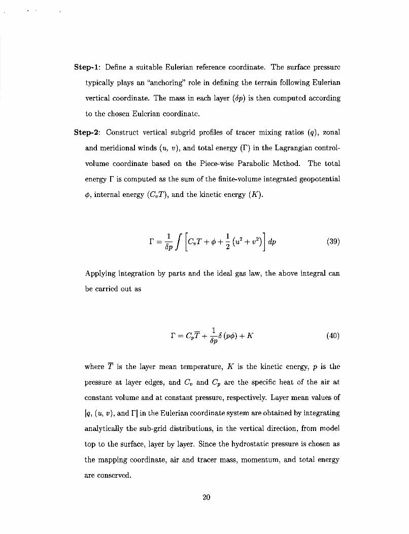
Step-2: Construct vertical subgrid profiles of tracer mixing ratios (a) , zonal

and meridional winds (u, v) , and total energy (I?) in the Lagrangian control-

volume coordinate based on the Piece-wise Parabolic Method. The total

energy is computed as the sum of the finite-volume integrated geopotential

4, internal energy (CUT), and the kinetic energy ( K ) .

Applying integration by parts and the ideal gas law, the above integral can

be carried out as

where T is the layer mean temperature, K is the kinetic energy, p is the

pressure at layer edges, and C, and C, are the specific heat of the air at

constant volume and at constant pressure, respectively. Layer mean values of

[q, (u, v) , and I?] in the Eulerian coordinate system are obtained by integrating

analytically the sub-grid distributions, in the vertical direction, from model

top to the surface, layer by layer. Since the hydrostatic pressure is chosen as

the mapping coordinate, air and tracer mass, momentum, and total energy

are conserved.

20

To convert the potential temperature 0 to the layer mean temperature the

conversion factor is obtained by equating the following two equivalent forms

of the hydrostatic relation.

64 = -GPO SrI

where ll = pn. The conversion formula between layer mean temperature and

layer mean potential temperatcure is

Slnp- 0 = K-T sn (43)

Step-3: Compute kinetic energy in the Eulerian coordinat system for each layer.

Substituting kinetic energy and the hydrostatic relationship (Eq. 42) into Eq.

40, the layer mean temperature for layer - IC in the Eulerian coordinate is

then retrieved from the reconstructed total energy (done in Step-2) by a fully

explicit integration procedure starting from the surface up to the model top

as follows:

21

The physical implication of retrieving the layer mean temperature from the total energy is

that the dissipated kinetic energy, if any, is locally converted into internal energy via the ver-

tically sub-grid mixing (dissipation) processes. Due to the monotonicity preserving nature of

the sub-grid reconstruction the column-integrated kinetic energy inevitably decreases (dis-

sipates), which leads to local frictional heating. The frictional heating is a physical process

that maintains the conservation of the total energy in a closed system.

As viewed by an observer riding on the Lagrangian surfaces, the mapping procedure

essentially performs the physical function of the relative-to-the-Eulerian-coordinate vertical

transport, by vertically redistributing mass, momentum, and total energy from the La-

grangian control-volume back to the Eulerian framework. The mapping time step can be

much larger than that used for the large-time-step tracer transport. In tests using the Held-

Sluarez forcing, a three-hour mapping time interval is found to be adequate. In the full model

i:ntegration, one may choose the same time step used for the physical parameterizations so

a s to ensure the input to physical parameterizations are in the usual “Eulerian” vertical co-

ordinate.

51. Idealized tests

We present results from two types of idealized tests. The first is a deterministic initial-value-

problem test case illustrating the growth and propagation of baroclinic instability initiated

hy a localized perturbation. The second is the “climate” simulation using the Held-Suarez

forcing. For both tests we used a 32-level hybrid o - p vertical coordinate as the “Eulerian”

coordinate for the mapping procedure. Below 500 mb, this 32-level setup is the same as the

PJCAR CCM3’s 18-level setup for climate simulations (Kiehl, et al. 1996). To better resolve

the stratosphere, the vertical resolution is substantially increased (as compared to CCM3)

near and above the tropopause level. The model top is located at 0.4 mb.

The initial condition for the baroclinic instability test case is specified analytically as

22

where

z = zog (;) ) Po = 1000 (mb), U" = 3574s

The mean flow, which is symmetric with respect to the equator, is in hydrostatic equilibrium

with the meridional wind being identically zero. The balanced zonal mean temperature is

then computed numerically. The base state thus constructed is a steady state solution to the

3D governing equations. To break the symmetry and to trigger the growth of the baroclinic

instability, a localized initial temperature perturbation centered at 45N and 90E is super-

i.mposed to the mean field. Previous theoretical studies (e.g., Lin and Pierrehumbert 1993)

indicated that the localized disturbance will propagate eastward while growing exponentially.

Due to nonlinearity and periodicity of the spherical geometry, the instability will saturate

and the perturbation will cycle zonally to become a global mode.

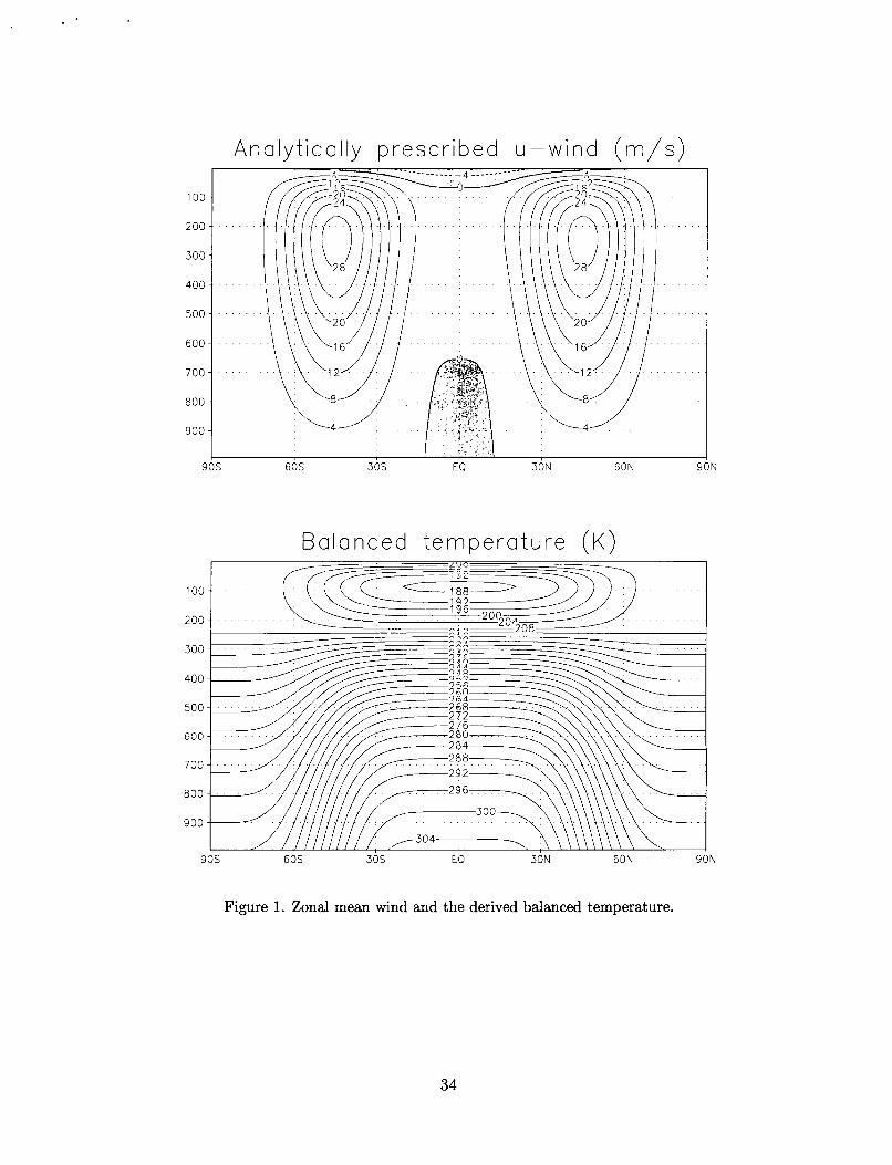
Figure 1 depicted the prescribed zonal mean wind and the derived balanced temperature.

The wind is a fairly realistic representation of the annual mean condition with the derived

temperature showing a cold tropical tropopause centered near 100 mb and with realistic

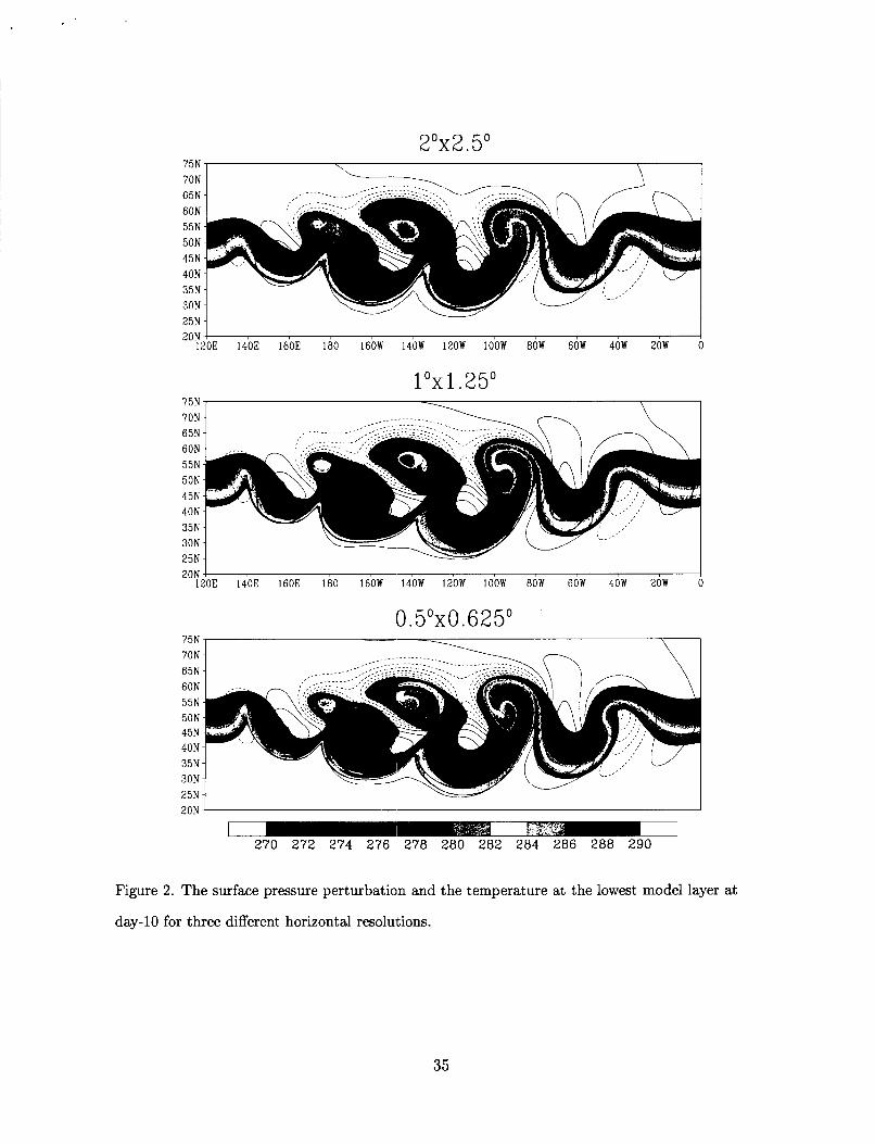
lapse rates throughout the globe. Experiments were carried out using three progressively

higher horizontal resolutions: one at 2" x 2.5" (denoted as B32), the second at 1" x 1.25"

(denoted as C32), and the third at 0.5" x 0.625" (denoted as D32), with small-time-step of

450 seconds, 225 seconds, and 112.5 seconds, respectively. The mapping time step is fixed

to be one hour for all presented tests.

Figure 2 compares, at day 10, the surface pressure perturbations and the temperature at

the model's lowest layer. It is seen that the phases of the propagation of the disturbances

23

agree remarkably well among all three resolutions. However, the amplitudes in the lower res-

olution runs are somewhat weaker. These are expected characteristics of the monotonicity-

preserving finite-volume algorithms. The initial-value problem tests offer no proof that the

simulations are “correct)’ or have converged. In fact, the results show that even at approx-

i:mately 55 km resolution the detailed features of the cyclones may still be under-resolved.

Nevertheless, a reasonable degree of convergence, particularly the large-scale features, has

been achieved, and there is no pathological amplification of the numerical noise in any resolu-

tions we tested. While a monotonicity-preserving algorithm is beneficial to scalar transport,

its advantage is unclear in climate simulations in which the preservation of variances is

regarded as more important. This issue is examined using the Held-Suarez forcing.

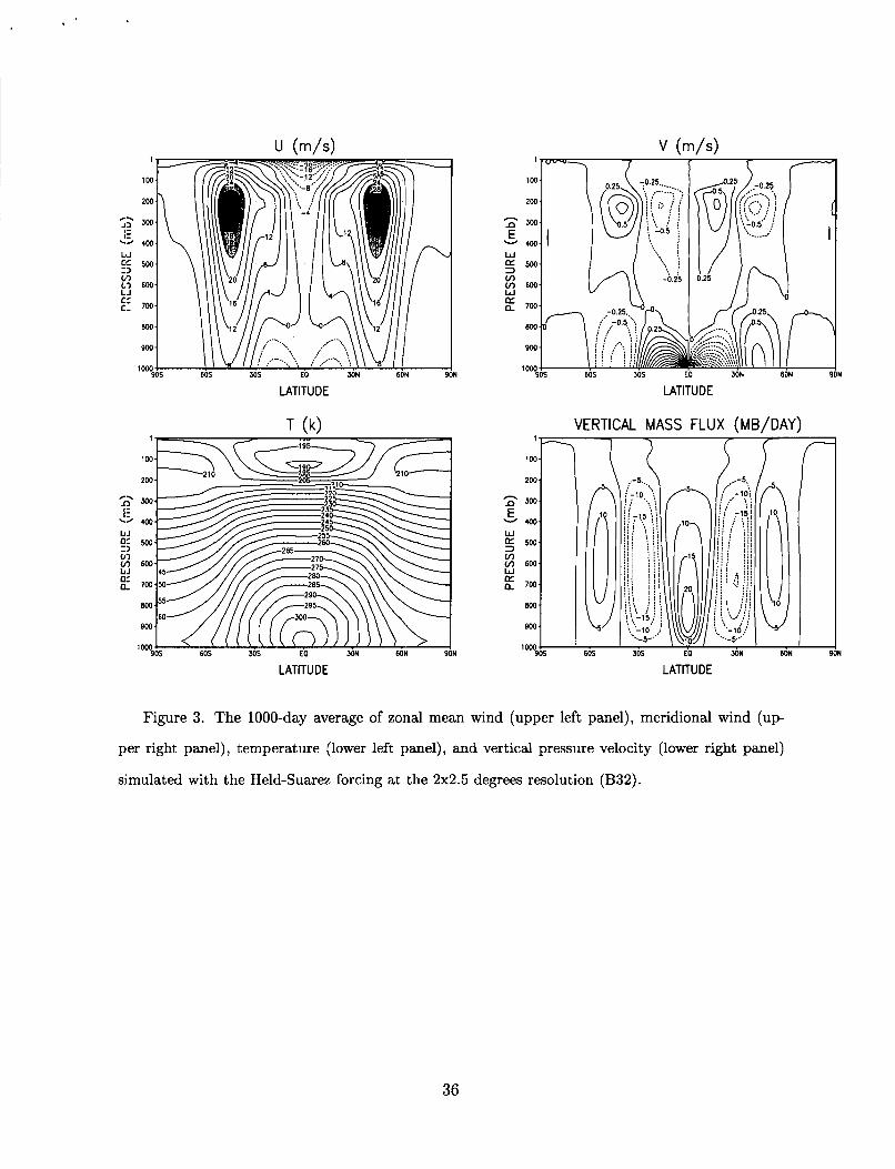
We applied the same initial condition used in the above tests to initialize the Held-Suarez

test. The integrations were carried out for more than four years. Statistics were computed

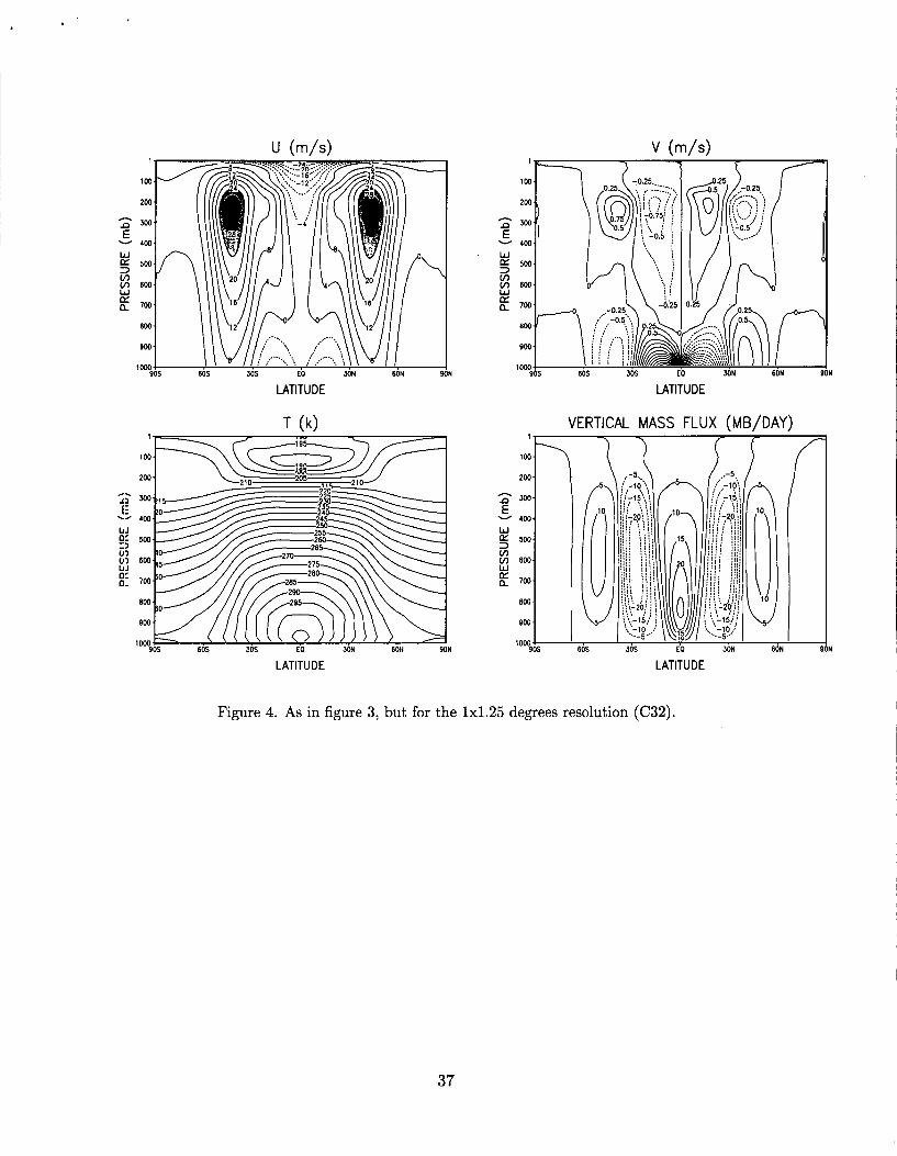
only for the last 1000 days. Figure 3 and figure 4 show, respectively, for the B32 and C32

resolutions, the zonal mean u-wind, v-wind, temperature, and the vertical pressure velocity.

Within the Lagrangian framework, the vertical pressure velocity is diagnosed as follows.

where the subscript IC indicates the ICth Lagrangian surface. pi+At is the pressure of the ICth

Lagrangian surface at time t + At before mapping (Lagrangian coordinate), p: is the value

a t time t immediately after the previous remapping (Eulerian coordinate), and At is the

mapping time step.

These zonal mean fields are in good agreement with Held and Suarez’s results. In par-

ticular, there is a distinct “tropical tropopause” of about 190 degree Kevin, and there is

also a cold surface layer. The simulated zonal mean flows are not exactly symmetric with

respect to the equator due to the asymmetric initial perturbation and the limited averaging

24

period. There are subtle differences between the two resolutions. Most notably the “trop-

ical tropopause” in the higher C32 resolution is a bit colder than that from the B32 case

whereas the polar “tropopause” (not clearly defined, but roughly at 250 mb level) in the

C32 is slightly warmer. The warming of the polar tropopause with increasing horizontal

resolution is consistent with full physics simulations using the CCM3 parameterizations (to

be presented by a follow up paper).

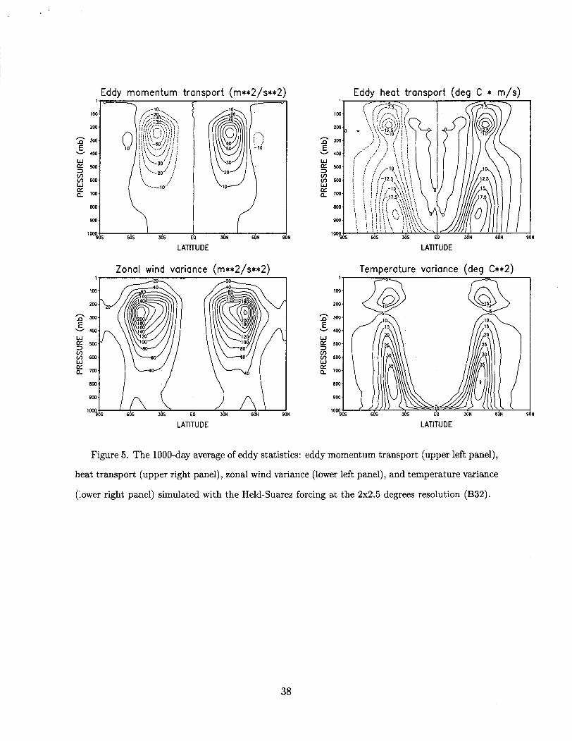
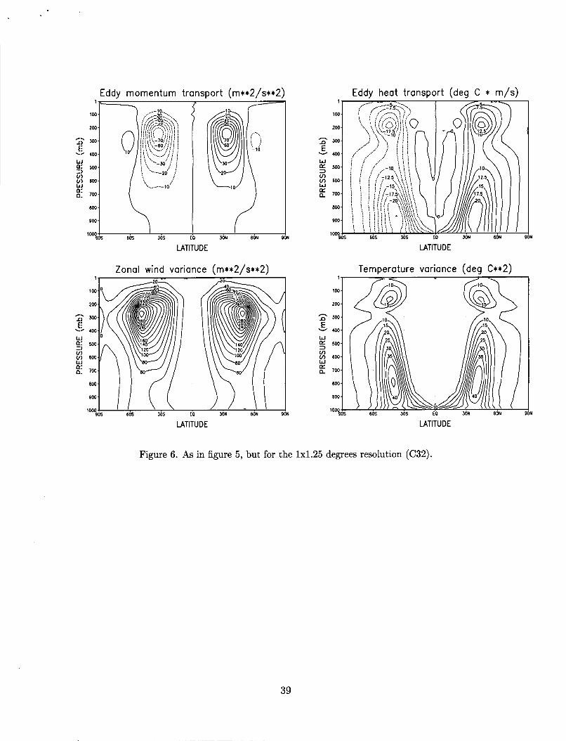
Figure 5 (for B32 case) and figure 6 (for C32 case) show the eddy momentum transport,

eddy heat transport, zonal wind variance, and the temperature variance, Except for the zonal

wind variance, a good degree of convergence has been achieved between the two resolutions.

However, the differences with Held-Suarez’s results were more pronounced in the second

moment statistics. For example, the temperature variances in our simulations show only a

single maxima in the upper troposphere of the midlatitudes whereas in the Held and Suzrez’s

results there is a secondary maxima, which could be of numerical origin.

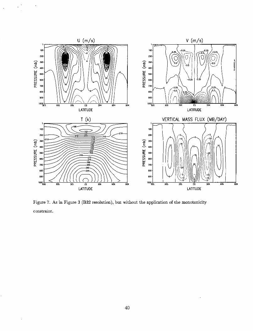
To examine the impacts of monotonicity constraint, which damps strongly the grid-

scale structures, to the simulated “climate”, we carried out another experiment with the

Ei32 resolution but without applying the monotonicity constraint to all horizontal transport

processes. Figure 7 and 8 show, respectively, the mean states and the eddy statistics. It is

seen that without the monotonicity constraint the simulation is, not surprisingly, closer to

the higher resolution (C32) case.

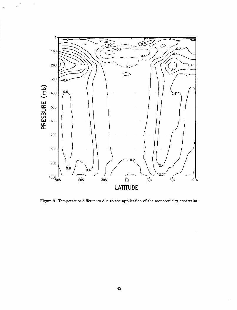
Figure 9 shows the differences in zonal mean temperature due to the monotonicity con-

straint. It indicates that, without the monotonicity constraint, poleward heat transport is

more rigorous, resulting in warmer poles and cooler tropics. The monotonicity constraint’s

seemingly negative impact to “climate simulations” needs to be re-examined in full model

simulations, which is beyond the scope of this paper. It is noted here that the monotonicity

constraint is highly desirable for the transport of water vapor, cloud water, and chemical

tracers to prevent the generation of negative values. In short-term deterministic initial-value

problems (e.g., weather predictions), it can be argued that elimination of grid-scale numeri-

25

cal noise is more important than the maintenance of variances. On the other hand, it may

be more important to preserve the variances in long term climate simulations.

ti. Concluding remarks

The finite-volume dynamical core described here has been successfully implemented into two

general circulation modeling systems, the NASA/NCAR general circulation model (fvGCM,

to be described elsewhere) and the Community Atmosphere Model (CAM). At the NASA

Data Assimilation Office (DAO), we have already successfully integrated the fvGCM into a

n.ew generation of the data assimilation system: the finite-volume Data Assimilation System

(fvDAS). Numerical weather prediction experiments using the fvGCM with initial conditions

produced by fvDAS indicated there is significant improvement in the forecast skill over DAO’s

previous operational system (GEOS-3 IIAS).

There are still some aspects of the numerical formulation in this dynamical core that can

be further improved. For example, the choice of the horizontal grid, the computational effi-

ciency of the split-explicit time marching scheme, the application of the various monotonicity

constraints, and how the conservation of total energy is achieved. The vertical Lagrangian

discretization with the associated remapping conserves the total energy exactly. The only

remaining issue regarding the conservation of the total energy is the use of the apparently

“(diffusive” monotonicity preserving transport scheme for the horizontal discretization.

The full impact of the non-linear diffusion associated with the monotonicity constraint

is difficult to access. All discrete schemes must address the problem of subgrid-scale mix-

ing. The non-linear diffusion in the finite-volume scheme creates strong local mixing when

monotonicity principles are violated. However, this local mixing diminishes quickly as the

resolution matches better to the spatial structure of the flow. In other numerical schemes,

however, an explicit (and tunable) linear diffusion is often added to the equations to provide

the subgrid-scale mixing as well as to smooth and/or stabilize the time marching.

26

To compensate for the loss of total energy due to horizontal discretization, one could apply

a, global fixer to add the loss in kinetic energy due to “diffusion” back to the thermodynamic

equation so that the total energy is conserved. However, our experience shows that even

without the “energy fixer” the loss in total energy (in flux unit) in a full GCM simulation is

less than 2 (W/m2) with the 2 degrees resolution, and much smaller with higher resolutions.

In the future, we may consider using the total energy as a prognostic variable so that the

total energy could be automatically conserved.

Extension of the algorithms described in this paper to unstructured grids is possible

but not straightforward. We are currently developing a high-order monotonicity preserving

finite-volume transport scheme for the Geodesic grid, which is to be used in the future de-

velopment of the finite-volume dynamical core, without the hydrostatic limitation.

tlcknowledgements. The author is indebted to Drs. R. B. Rood and R. Atlas for their

continued supports and encouragements during the development of the finite-volume

General Circulation Model. The author also thanks Dr. K.-S. Yeh and W. Putman for

proof reading the manuscript.

27

Appendix: Monotonicity constraints for PPM

The original Piecewise parabolic Method (PPM) as described by Colella and Woodward

(1984) has been modified to improve its computational performance and to reduce the nu-

merical diffusion. The PPM is built on the second order van Leer scheme. Given the

cell-mean value qi and assuming uniform grid spacing, the “mismatch” (Lin et al. 1994) of

the piecewise linear distribution is determined as

AqTmO = sign [vain( IAqi I , A q y , AqYax), Aqi]

where

1 AQi = 4 (Qi+l - Qi-1)

max - mzn - AQi - m4qi-1, Qi, Qi+l) - Qi , A4.i ‘ - Qi - min(qi-1, Qz, Qi+l)

To uniquely determined a parabolic polynomial within the finite-volume, in addition to

the volume mean value, the values at both edges of the parabola must be determined. The

first guess value at the left edge of the piecewise parabolic distribution is computed as

By continuity, the right edge value of cell (i) is simply the left-edge value of cell ( if l) .

That is, Q: = qZql. The application of a monotonicity constraint breaks the continuity of the

28

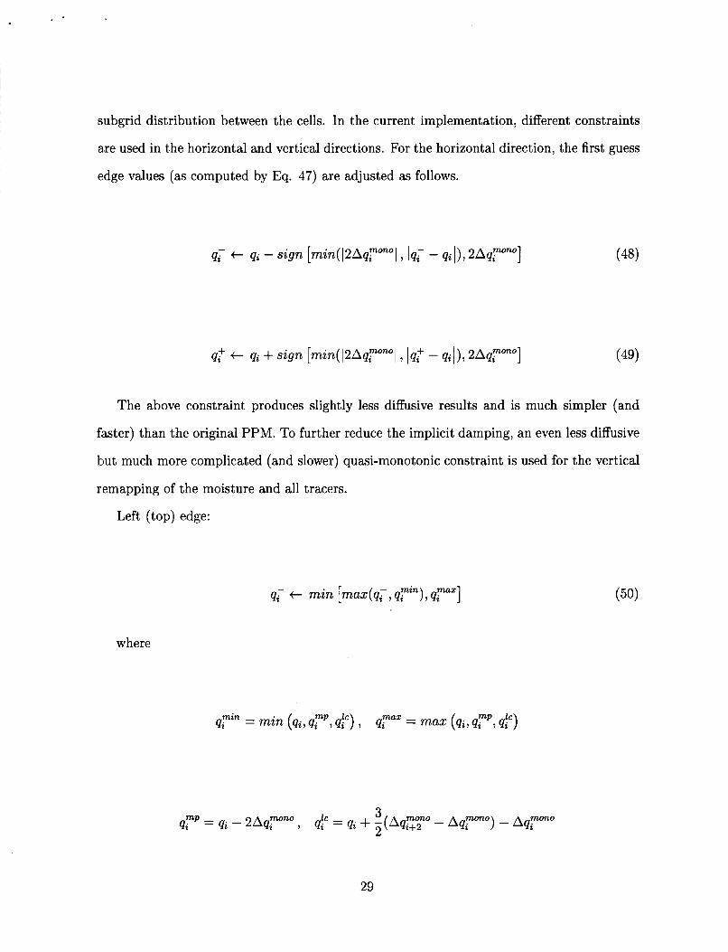
subgrid distribution between the cells. In the current implementation, different constraints

are used in the horizontal and vertical directions. For the horizontal direction, the first guess

edge values (as computed by Eq. 47) are adjusted as follows.

The above constraint produces slightly less diffusive results and is much simpler (and

faster) than the original PPM. To further reduce the implicit damping, an even less diffusive

hut much more complicated (and slower) quasi-monotonic constraint is used for the vertical

remapping of the moisture and all tracers.

Left (top) edge:

where

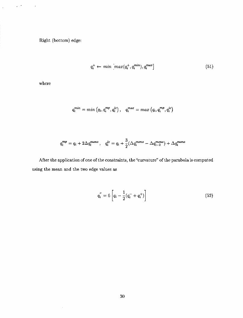
Right (bottom) edge:

where

After the application of one of the constraints, the “curvature” of the parabola is computed

u.sing the mean and the two edge values as

[ : q: = 6 qi - -(qc +q:)]

30

References

Allen, D. J., A. R. Douglas, R. B. Rood, and P. D. Guthrie, 1991: Application of a monotonic

upstream-biased transport scheme to three-dimensional constituent transport calculations.

Mon. Wea. Rev., 119, 26-2464.

Allen, D. J., P. J. Kasibhatla, A. M. Thompson, R. B. Rood, B. G. Doddridge, K. E. Pickering, R.

D. Hudson, and S.-J. Lin, 1996: Transport induced interannual variability of carbon monoxide

determined using a chemistry and transport model. J. Geophys. Res., 101, 28655-28669.

Arakawa, A and V. R. Lamb, 1981: A potential enstrophy and energy conserving scheme for the

shallow-water equations. Mon. Wea. Rev., 109, 18-36.

Carpenter, R. L., K. K. Drogemeier, P. R. Woodward, and C. E. Hane, 1990: Application of the

piecewise parabolic method to meteorological modelling. Mon. Wea. Rev., 118, 586-612.

Colella, P., and P. R. Woodward, 1984: The piecewise parabolic method (PPM) for gas-dynamical

simulations. J. Comput. Phys., 54, 174-201.

Held, I. M., and M. J. Suarez, 1994: A proposal for the intercomparison of the dynamical cores of

atmospheric general circulation models. BUZZ. Amer. Meteor., 751825-1830.

Hsu, Y.-J. G., and A. Arakawa, 1990: Numerical modeling of the atmosphere with an isentropic

vertical coordinate. Mon. Wea. Rev., 118, 1933-1959.

Kasahara, A., 1974: Various vertical coordinate systems used for numerical weather prediction.

Mon. Wea. Rev., 102, 504-522.

Kiehl, J. T., J. J. Hack, G. B. Bonan, B. A. Boville, B. P. Briegleb, D. L. Williamson, and P. J.

Rasch 1996: Description of the NCAR Community Climate Model (CCM3). NCAR Technical

Note, NCAR/TN-@O+STR, Boulder, CO, 152pp.

Lin, S.-J., and R. T. Pierrehumbert, 1993: Is the mid-latitude zonal flow absolutely unstable? J.

Atmos. Sci., 51, 1282-1297.

31

Lin, S.-J., W. C. Chao, Y. C. Sud, and G. K. Walker, 1994: A class of the van Leer-type transport

schemes and its applications to the moisture transport in a general circulation model. Mon.

Wea. Rev., 122, 1575-1593.

Lin, S.-J., and R. B. Rood, 1996: Multidimensional Flux Form Semi-Lagrangian Transport schemes.

Mon. Wea. Rev., 124, 2046-2070.

Lin, S.-J., 1997: A finite-volume integration method for computing pressure gradient forces in

general vertical coordinates. Q. J. Roy. Met. SOC., 123, 1749-1762.

Lin, S.-J., and R. B. Rood, 1997: An explicit flux-form semi-Lagrangian shallow water model on

the sphere. Q. J . Roy. Met. SOC., 123, 2531-2533.

Lin, S.-J., 1998: Reply to comments by T. Janjic on "A finite-volume integration method for

computing pressure gradient forces in general terrain-following coordinates". Q. J . Roy. Met.

Soc., 124, 1749-1762.

Lin, S.-J., and R. B. Rood, 1998: A flux-form semi-Lagrangian general circulation model with

a Lagrangian control-volume vertical coordinate. The Rossby-100 symposium, Stockholm,

Sweden.

Lin, S.-J., and R. B. Rood, 1999: Development of the joint NASA/NCAR General Circulation

Mode. Preprint, 13th conference o n Numerical Weather Prediction, Denver, CO.

Randall, D. A., 1994: Geostrophic adjustment and the finite-difference shallow-water equations.

Mon. Wea. Rev., 122, 1371-1377.

Ringler, T. D., R. P. Heikes, and D. A. Randall, 2000: Modeling the atmospheric general circulation

using a spherical geodesic grid: A new class of dynamical cores. Mon. Wea. Rev., 128, 2471-

2490.

Rood, R. B., 1987: Numerical advection algorithms and their role in atmospheric transport and

chemistry models. Rev. Geophys., 25, 71-100.

32

Rotman, D., J. Tannahill, D. Kinnison, P. Connell, Bergmann, Proctor, J. Rodriguez, S.-J. Lin,

R. B. Rood, M. Prather, P. Rasch, D. Considine, R. Ramaroson, R. Kawa, 2001: Global

Modeling Initiative Assessment Model: Model description, integration and testing of the

transport shell. J. Geophys. Res., Vol. 106, No. D2, 1669-1691.

Starr, V. P., 19: A quasi-Lagrangian system of hydrodynamical equations. J. Meteor., 2, 227-237.

Suarez, M. J., and L. L. Takacs: Documentation of the ARIES/GEOS dynamicd core: Version 2.

NASA Technical Memorandum, 104 606, Vol. 5.

Van Leer, B., 1977: Toward the ultimate conservative difference scheme. Part IV: A new approach

to numerical convection. J. Comput. Phys., 23, 276-299.

Woodward, P. R., and P. Colella, 1984: The numerical simulation of two-dimensional fluid flow

with strong shocks. J. Comput. Phys., 54, 115-173.

33

Analy t ica l ly p r e s c r i b e d u - w i n d ( m / s )

100

200

300

400

500

600

700

800

900

s

100

200

300

400

500

600

700

800

900

9

605 305 EQ 30N 60N E

B a l a n c e d t e m p e r a t u r e (K )

N

300

~ 3 0 4

> 605 305 EQ 30N 60N 90N

Figure 1. Zonal mean wind and the derived balanced temperature.

34

2'x2.5' 70N 4 L\ ', I ............. --. ...... ... .. ............... (;r;;;;; .... C..'. I ...= ::. .....: :. :-

lox 1.25'

............ 65N ..............

........................ .............. ..-:--.. \ I n _, ~

I , ,.-,;I :;: :.:.:.=.:.:.:-:-: f:: .:-. .

;:;I , - & & - 25N 20N

120E 140E 160E 180 160W 140W 120W lOOW 8OW 60W 40W 20W 0

0.5'xO. 625' 75N I \ I

...... 65N - - - \ I

20N ' I

270 272 274 276 278 280 282 284 286 288 290

Figure 2. The surface pressure perturbation and the temperature at the lowest model layer at

day-10 for three different horizontal resolutions.

35

LATITUDE

T (k)

LATlTU DE

LATITUDE

VERTICAL MASS FLUX (MB/DAY) 1 I i r

LATITUDE

I 60N <

Figure 3. The 1000-day average of zonal mean wind (upper left panel), meridional wind (up

per right panel), temperature (lower left panel), and vertical pressure velocity (lower right panel)

si.mulated with the Held-Suarez forcing at the 2x2.5 degrees resolution (B32).

IN

36

LATlTU D E LATITUDE

VERTICAL MASS FLUX (MB/OAY)

LATITUDE LATITUDE

Figure 4. As in figure 3, but for the 1x1.25 degrees resolution (C32)

37

Eddy momentum transport (m**2/s**2)

I

Eddy heat transport (deg C * m/s)

900 f Zonal wind variance (m**2/s**2)

LATITUDE

LATITUDE

Temperature variance (deg C**2) 1,

LATITUDE

Figure 5. The 1000-day average of eddy statistics: eddy momentum transport (upper left panel),

heat transport (upper right panel), zonal wind variance (lower left panel), and temperature variance

(lower right panel) simulated with the Held-Suarez forcing at the 2x2.5 degrees resolution (B32).

38

Eddy momentum transport (m**Z/s**Z I--

@) 20 10

I 66s 305 EP 30N 6ON

1WO 90s

LATITUDE

Zonal wind variance (m**Z/s**Z)

Eddy heat transport (deg C * m/s)

, LATITUDE

Temperature variance (deg C**Z)

LATITUDE LATITUDE

Figure 6. As in figure 5, but for the 1x1.25 degrees resolution (C32).

39

LATITUDE LATITUDE

VERTICAL MASS FLUX (MB/DAY)

LATITUDE

Figure 7. As in Figure 3 (B32 resolution), but without the application of the monotonicity

constraint.

40

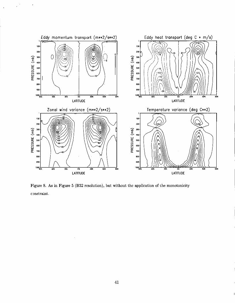
Eddy momentum transport (m**2/s**2)

'., 0

10

I EG5 30s LP M N 60N 4

LATITUDE

Zonal wind variance (m**2/s**2)

Eddy heat transport (deg C * m/s)

LATITUDE

Temperature variance (deg C**2) 1

LATITUDE LATITUDE

Figure 8. As in Figure 5 (B32 resolution), but without the application of the monotonicity

c'onstraint .

41

N

LATlTU DE

Figure 9. Temperature differences due to the application of the monotonicity constraint.

42