Aberration TheoryMade Simple

Second Edition

Errata to First Printing

Corrections are highlighted or otherwise marked in the following pages.

PREFACE TO THE SECOND EDITION

I wrote Aberration Theory Made Simple some 20 years ago to provide a clear,

concise, and consistent exposition of what aberrations are, how they arise in optical

imaging systems, and how they affect the quality of optical images formed by them, both

in terms of geometrical and diffraction optics. Later, I expanded this Tutorial Text into a

textbook under the title Optical Imaging and Aberrations in two parts, one on Ray

Geometrical Optics and the other on Wave Diffraction Optics. Detailed mathematical

derivations missing in the Tutorial Text are given in this textbook, along with problems at

the end of each chapter.

In this second edition of Aberration Theory Made Simple, I have updated the sign

convention for Gaussian optics to the Cartesian sign convention, as used in advanced

books on geometrical optics and in the optical design software programs. The quantities

such as object and image distances that are numerically negative are indicated in figures

with a parenthetical negative sign (–). Thus a reader will find a change in the sign of

some parameters in equations in the part on geometrical optics when compared with those

in the first edition. In this new edition, I have deleted certain advanced details that are

available in the long textbook. Deletions include the plots of the optical transfer function

for primary aberrations. I have added some new material as well, such as the centroid and

standard deviation of ray aberrations, spot diagrams for primary aberrations, golden rule

of optical design about relying on such diagrams, update of 2D PSFs for primary

aberrations, aberration-free optical transfer function of systems with annular and

Gaussian pupils, Zernike polynomials for circular pupils and the corresponding

polynomials for annular and Gaussian pupils, effect of longitudinal image motion on an

image, lucky imaging in ground-based astronomy, and adaptive optics. I have also added

a brief summary at the end of each chapter, highlighting the essence of its content. It is

hoped that these additions will be helpful to the readers of this edition of Aberration

Theory Made Simple.

The second edition of Aberration Theory Made Simple has been translated into

Russian by Professor Irina Livshit� of National Research University of Information

Technologies, �Mechanics and �Optics, Saint Petersburg, Russia. This Russian edition is

available from the university by contacting her at <ecenter-optica10@yandex.ru>.

Virendra N. Mahajan June 2011

El Segundo, California

xv

Livshit�

1.5 Wavefront Tilt 7

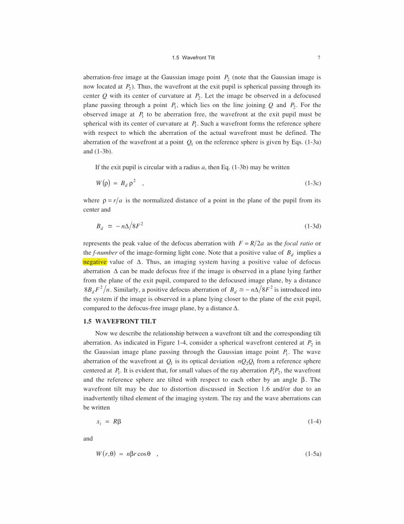
aberration-free image at the Gaussian image point P2 (note that the Gaussian image is

now located at P2). Thus, the wavefront at the exit pupil is spherical passing through its

center Q with its center of curvature at P2. Let the image be observed in a defocused

plane passing through a point P1, which lies on the line joining Q and P2. For the

observed image at P1 to be aberration free, the wavefront at the exit pupil must be

spherical with its center of curvature at P1. Such a wavefront forms the reference sphere

with respect to which the aberration of the actual wavefront must be defined. The

aberration of the wavefront at a point Q1 on the reference sphere is given by Eqs. (1-3a)

and (1-3b).

If the exit pupil is circular with a radius a, then Eq. (1-3b) may be written

W Bdr r( ) = 2 , (1-3c)

where r = r a is the normalized distance of a point in the plane of the pupil from its

center and

B n Fd ~ - D 8 2 (1-3d)

represents the peak value of the defocus aberration with F R a= 2 as the focal ratio or

the f-number of the image-forming light cone. Note that a positive value of Bd implies a

negative value of D . Thus, an imaging system having a positive value of defocus

aberration D can be made defocus free if the image is observed in a plane lying farther

from the plane of the exit pupil, compared to the defocused image plane, by a distance

8 2B F nd . Similarly, a positive defocus aberration of B n Fd ~ - D 8 2 is introduced into

the system if the image is observed in a plane lying closer to the plane of the exit pupil,

compared to the defocus-free image plane, by a distanceD .

1.5 WAVEFRONT TILT

Now we describe the relationship between a wavefront tilt and the corresponding tilt

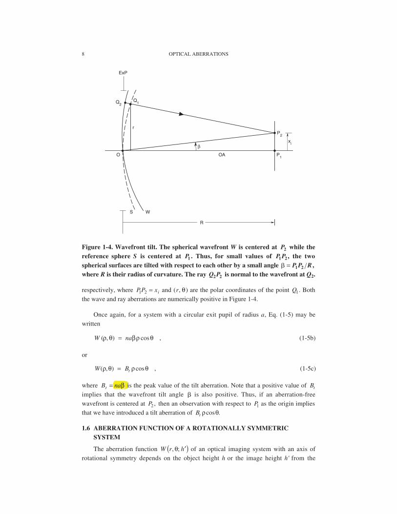
aberration. As indicated in Figure 1-4, consider a spherical wavefront centered at P2 in

the Gaussian image plane passing through the Gaussian image point P1. The wave

aberration of the wavefront at Q1 is its optical deviation nQ Q2 1 from a reference sphere

centered at P1. It is evident that, for small values of the ray aberration P P1 2 , the wavefront

and the reference sphere are tilted with respect to each other by an angle b . The

wavefront tilt may be due to distortion discussed in Section 1.6 and/or due to an

inadvertently tilted element of the imaging system. The ray and the wave aberrations can

be written

x Ri = � (1-4)

and

W r n r, cos ,q b q( ) = (1-5a)

negative

8 OPTICAL ABERRATIONS

ExP

WS

R

P1

P2

Q1Q

2

r

O OA

bx

i

Figure 1-4. Wavefront tilt. The spherical wavefront W is centered at P2 while thereference sphere S is centered at P1 . Thus, for small values of P P1 2 , the twospherical surfaces are tilted with respect to each other by a small angle � = P P R1 2 ,where R is their radius of curvature. The ray Q P2 2 is normal to the wavefront at Q2.

respectively, where P P xi1 2 = and (r, q) are the polar coordinates of the point Q1. Both

the wave and ray aberrations are numerically positive in Figure 1-4.

Once again, for a system with a circular exit pupil of radius a, Eq. (1-5) may be

written

W na( , ) cos ,r q br q= (1-5b)

or

W Bt( , ) cos ,r q r q= (1-5c)

where B nat = b is the peak value of the tilt aberration. Note that a positive value of Bt

implies that the wavefront tilt angle � is also positive. Thus, if an aberration-free

wavefront is centered at P2 , then an observation with respect to P1 as the origin implies

that we have introduced a tilt aberration of Bt r qcos .

1.6 ABERRATION FUNCTION OF A ROTATIONALLY SYMMETRIC SYSTEM

The aberration function W r h, ;q ¢( ) of an optical imaging system with an axis of

rotational symmetry depends on the object height h or the image height h' from the

ibna

CHAPTER 2Thin Lens2.1 INTRODUCTION

Among the simple optical imaging systems, a thin lens consisting of two spherical

surfaces is the most common as well as practical. By applying the results of Section 1.8

and the procedure of Section 1.9, we give the imaging equations and expressions for the

primary aberrations of a thin lens with aperture stop located at the lens. Its aberrations for

other locations of the aperture stop may be obtained by applying the results of Section 1.7

to those given here. It is shown that when both an object and its image are real, the

spherical aberration of a thin lens cannot be zero (unless its surfaces are made

nonspherical). We illustrate by a numerical example, however, that it is possible to design

a two-lens combination such that its spherical aberration and coma are both zero. In such

a combination, these aberrations associated with one lens cancel the corresponding

aberrations of the other. This cancellation is illustrated with a numerical example.

2.2 GAUSSIAN IMAGING

Consider a thin lens of refractive index n and focal length ¢f consisting of two

spherical surfaces of radii of curvature R1 and R2 as illustrated in Figure 2-1. A lens is

considered thin if its thickness is negligible compared to ¢f , R1, and R2 . Its optical axis

OA is the line joining the centers of curvature C1 and C2 of its surfaces. Since the lens is

thin, we neglect the spacing between its surfaces. We assume that its aperture stop AS is

located at the lens, so that its entrance and exit pupils EnP and ExP, respectively, are also

located there. The lens is located in air; therefore, the refractive index of the surrounding

medium is 1.

Consider a point object P located at a distance S from the lens and at a height h from

its axis. The first surface forms the image of P at ¢P and the second surface forms the

image of ¢P at ¢¢P . Applying the results of Section 1.8 to imaging by the two surfaces of

the lens, where n = 1 and ¢ =n n for the first surface and n n= and ¢ =n 1 for the second

surface, we can show that the image distance ¢S and its height ¢h are given by the

relations

1 11

1 1

1 2¢- = -( ) -

ÊËÁ

ˆ¯̃S S

nR R

(2-1a)

=¢

1

f(2-1b)

and

Mh

h=

¢=

¢S

S, (2-2)

19

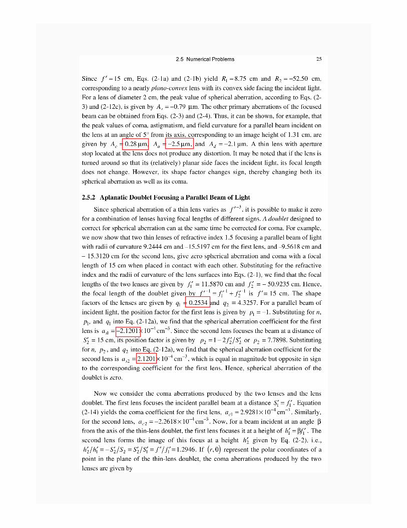
26 THIN LENS

W r a h rc c1 1 13, cosq q( ) = ¢

= ¥ ¢-2 2618 10 42

3. cosh r q (2-17a)

and

W r a h rc c2 2 23, cosq q( ) = ¢

= - ¥ ¢-2 2618 10 42

3. cos .h r q (2-17b)

The coma aberration of the lens doublet is given by

W r W r W rc c c, , ,q q q( ) = ( ) + ( )1 1 = 0 . (2-18)

Thus, both spherical aberration and coma of the doublet are zero. Such a system is called

aplanatic.

Finally, we consider the astigmatism and field curvature aberrations of the lens

doublet. Substituting for the focal length and the image distance for the two lenses in Eq.

(2-4c), we obtain their astigmatism coefficients aa143 2141 10= - ¥ - -. cm 3 and

aa254 3638 10= ¥ - -. cm 3 . Hence, astigmatism aberration of the doublet at a point r,q( )

in its plane may be written

W r h W r h W r ha a a, ; , ; , ;q q q¢( ) = ¢( ) + ¢( )2 1 1 2 2

= ¢ + ¢a h r a h ra a1 12 2 2

2 22 2 2cos cosq q

= +( ) ¢0 5967 1 2 22 2 2. cosa a h ra a q

= - ¥ ¢-1 4815 10 42

2 2 2. cos .h r q (2-19)

For a beam incident on the doublet at an angle of 5° from its axis, we obtain ¢ =h2 1 31.

cm. Hence, for a beam of diameter 2 cm, the peak value of astigmatism aberration is

approximately given by Aa = -2 54. m m. Comparing Eqs. (2-4c) and (2-4d), the

corresponding field curvature aberration may be obtained from Aa by multiplying it by

n n+( )1 2 . Thus, we find that Ad = -2 12. mm.

2.6 SUMMARY

A thin lens generally consists of two spherical surfaces with negligible thickness.

The spherical aberration of such a thin lens cannot be zero when an object and its image

are both real. However, since this aberration varies as the cube of the lens focal length, it

can be made zero by combining two lenses of focal lengths with opposite signs. The

doublet, as it is called, can also be made coma free, and the system is then referred to as

being aplanatic.

3 2141-3 214121412141

= --2 5454

--2 12.

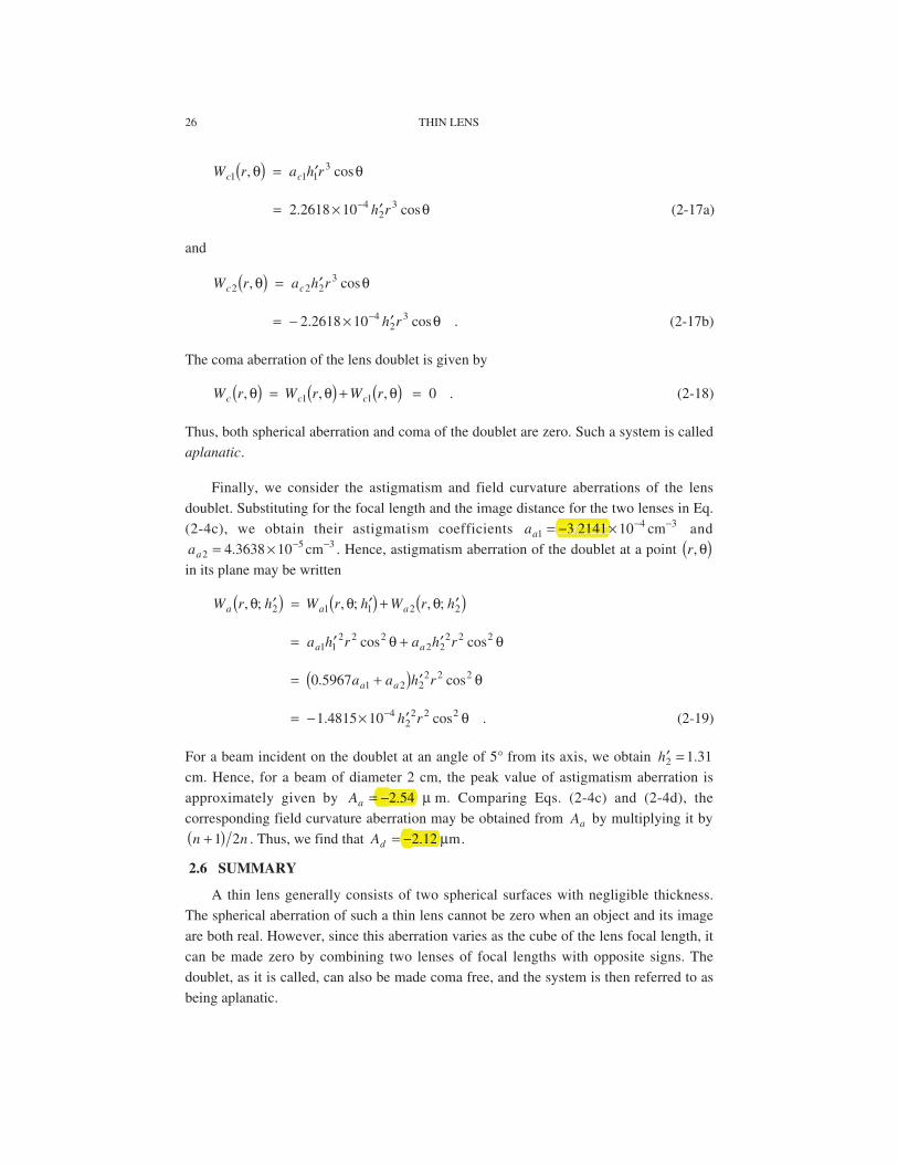
30 ABERRATIONS OF A PLANE-PARALLEL PLATE

Finally, we combine the aberrations introduced by the two surfaces to obtain the

aberration introduced by the plate. Since m2 and M2 are both unity, r r1 1 2 2, ,q q( ) = ( ) and

¢ = ¢ =h h h2 1 , respectively. Hence, following Eq. (1-29), the aberration of the plane-

parallel plate at a point r, q( ) in the plane of its exit pupil can be written

W r h W r h W r h, ; , ; , ; .q q q( ) = ( ) + ( )1 2 (3-12)

Substituting Eqs. (3-8) and (3-10) into Eq. (3-12), we may write the primary aberration

function

W r h a r hr h r h r h rs, ; cos cos cos ,q q q q( ) = - + + -( )4 3 2 2 2 2 2 34 4 2 4 (3-13)

where

a a S L as s s= + ¢( )1 2 24

2 . (3-14)

Substituting Eqs. (3-1), (3-3), (3-6b), (3-7), and (3-9) into Eq. (3-14), we obtain

an t

n Ss =-( )2

3 4

1

8. (3-15)

Note that the aberration increases linearly with the plate thickness t. Moreover, as

expected, the aberration reduces to zero for a collimated incident beam ( )S Æ - • . This

is indeed why a lens designer places beam splitters and windows in an imaging system in

its collimated spaces wherever possible.

3.4 NUMERICAL PROBLEM

As a numerical example we determine the aberrations of a plane-parallel plate placed

in the path of a converging beam as shown in Figure 3-2. The plate has a refractive index

of 1.5. Its thickness is 1 cm and its diameter is 4 cm. In the absence of the plate, the beam

comes to a focus at P at a distance of 8 cm from its front surface at a height of 0.5 cm

from its axis. From Eq. (3-5), we find that the plate displaces the image from P to ¢P

which is at the same height as P but at a distance of 8.33 cm from its front surface.

Substituting for n, t, and S = 8 cm in Eq. (3-15), we obtain as = ¥ - -1 13 10 5 3. cm . Noting

that the maximum value of r is 2 cm, we obtain the peak values of the primary aberrations

introduced by the plate from Eq. (3-13); As = 1 81. mm, Ac = -1 81. mm, Aa = 0 45. mm,

Ad = 0 23. mm, and At = -0 11. mm.

3.5 SUMMARY

A plane-parallel plate is often used in imaging systems as a beam splitter or a

window. It introduces no aberrations when placed in a collimated space. However, it

introduces aberrations when placed in a converging or a diverging beam of light. The

primary aberrations thus introduced are given by Eq. (3-13). They increase linearly with

the thickness of the plate.

-10 5-5= 1.13¥

0 45m--1 81m= 1 81m--0 111m0 233m

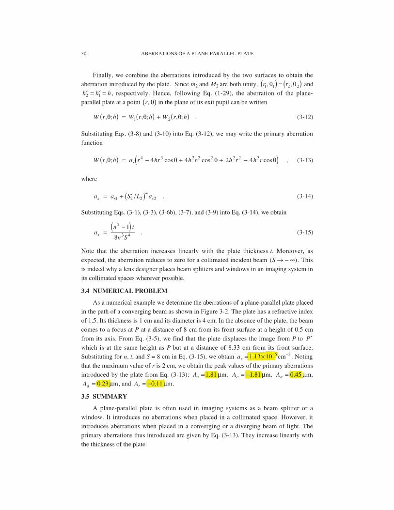
40 ABERRATIONS OF A SPHERICAL MIRROR

Table 4-2. Gaussian and aberration parameters for a spherical mirror imaging anobject lying at infinity at an angle of 1 milliradian from its optical axis. The aperturestop is located at the mirror.

Gaussian Parameters

Mirror R(cm)

¢S(cm)

¢h(cm)

F d

Concave –10 –5 5 10 3¥ - 1.25 –2

Convex 10 5 - ¥ -5 10 3 1.25 –2

Aberration Parameters

Mirror ass

cm 3-( )Ass

mmm( )Acs

mmm( )Aas

mmm( )

Concave - ¥ -2 5 10 4. - 40 0.8 - ¥ -4 10 3

Convex - ¥ -2 5 10 4. 40 0.8 4 10 3¥ -

Table 4-3. Radius of the exit pupil and field curvature parameters for a sphericalmirror when the aperture stop is located at its center of curvature.*

Mirror aex

(cm)

ad

cm 3-( )Ad

mmm( )

Concave 2 3

(2)

8 10 3¥ -

2 10 3¥( )-

35.6

2 10 3¥( )-

Convex 10 3

(2)

- ¥ -1 28 10 3.

- ¥( )-2 10 3

–35.6

- ¥( )-2 10 3

* The numbers without parentheses are for an object at S = 15 cm and those with

parentheses are for an object at infinity at 1 milliradian from the optical axis of the

system.

4

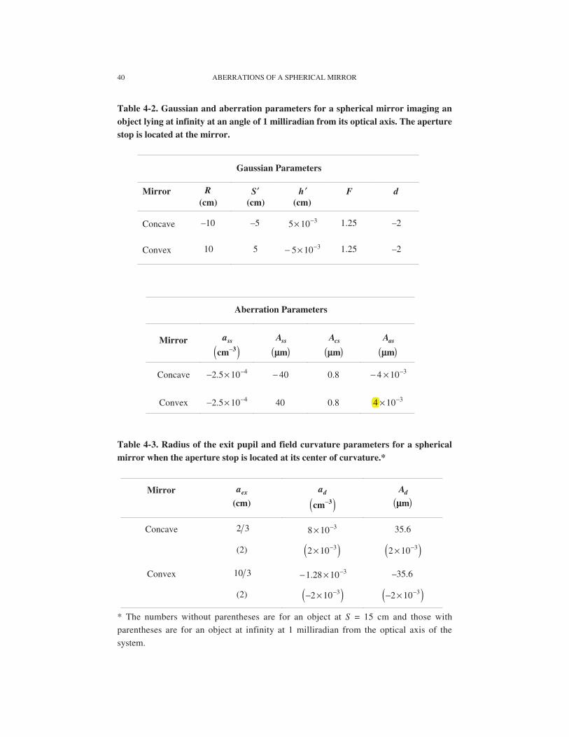
64 RAY SPOT SIZES AND DIAGRAMS

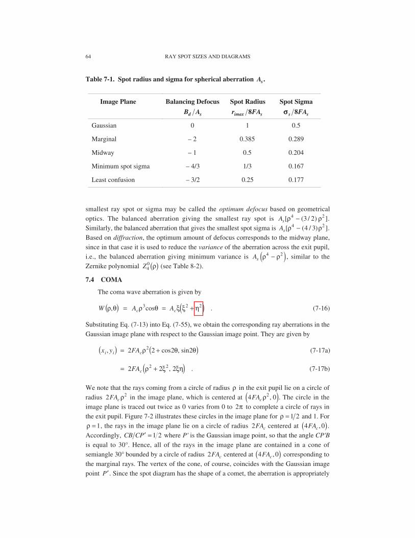
Table 7-1. Spot radius and sigma for spherical aberration As .

Image Plane Balancing Defocus

B Ad s

Spot Radius

r FAimax s8

Spot Sigma

ss s sFA8

Gaussian 0 1 0.5

Marginal – 2 0.385 0.289

Midway – 1 0.5 0.204

Minimum spot sigma – 4/3 1/3 0.167

Least confusion – 3/2 0.25 0.177

smallest ray spot or sigma may be called the optimum defocus based on geometrical

optics. The balanced aberration giving the smallest ray spot is As[ ( / ) ]r r4 23 2- .

Similarly, the balanced aberration that gives the smallest spot sigma is As[ ( / ) ]r r4 24 3- .

Based on diffraction, the optimum amount of defocus corresponds to the midway plane,

since in that case it is used to reduce the variance of the aberration across the exit pupil,

i.e., the balanced aberration giving minimum variance is As r r4 2-( ) , similar to the

Zernike polynomial Z40 r( ) (see Table 8-2).

7.4 COMA

The coma wave aberration is given by

W A Ac cr q r q x x h, .( ) = = +( )3 2 2cos (7-16)

Substituting Eq. (7-13) into Eq. (7-55), we obtain the corresponding ray aberrations in the

Gaussian image plane with respect to the Gaussian image point. They are given by

x y FAi i c, ,( ) = +( )2 2 2 22r q qcos sin (7-17a)

, .= +( )2 2 22 2FAc r x xh (7-17b)

We note that the rays coming from a circle of radius r in the exit pupil lie on a circle of

radius 2 2FAcr in the image plane, which is centered at 4 02FAcr ,( ). The circle in the

image plane is traced out twice as 0 varies from 0 to 2p to complete a circle of rays in

the exit pupil. Figure 7-2 illustrates these circles in the image plane for r = 1 2 and 1. For

r = 1, the rays in the image plane lie on a circle of radius 2FAc centered at 4 0FAc ,( ) .

Accordingly, CB CP¢ = 1 2 where P' is the Gaussian image point, so that the angle CP'B

is equal to 30°. Hence, all of the rays in the image plane are contained in a cone of

semiangle 30° bounded by a circle of radius 2FAc centered at 4 0FAc ,( ) corresponding to

the marginal rays. The vertex of the cone, of course, coincides with the Gaussian image

point ¢P . Since the spot diagram has the shape of a comet, the aberration is appropriately

66 RAY SPOT SIZES AND DIAGRAMS

x y FAc c c, , .( ) = ( )2 0 (7-18)

Thus, the centroid lies at the point S in Figure 7-2 where the sagittal marginal rays

intersect the image plane. Substituting Eqs. (7-17) and (7-18) into Eq. (7-8a), we obtain

the ray spot sigma:

s r q r qs cFA= +( ) -[ ] +2 2 2 1 22 2 4 21 2

cos sin

= 2 2 3FAc . (7-19)

Measuring the ray coordinates in the image plane with respect to a point other than

the Gaussian image point is equivalent to introducing a wavefront tilt aberration in the

aberration function. A tilt aberration with a peak value of At is equivalent to measuring

the wave aberration with respect to a reference sphere centered at a point in the image

plane with coordinates -( )2 0FAt , . Hence, measuring the ray aberrations with respect to

the centroid is equivalent to a tilt aberration of -Acr qcos or A At c= - . Accordingly, the

aberration function with respect to the centroid can be written

W Acr q r r q, cos .( ) = -( )3 (7-20)

It should be evident that if the ray aberrations are measured with respect to any other

point in the image plane, including the Gaussian image point, the spot sigma will

increase. The aberration function given by Eq. (7-20) represents coma aberration

balanced optimally with tilt aberration to yield minimum sigma value or bring the

centroid at the Gaussian image point. However, the variance of the wave aberration is

minimum when A At c= -( )2 3 , i.e., if the balanced aberration is Ac r r q3 2 3-[ ]( / ) cos ,

similar to the Zernike polynomial Z31 r q,( ) .

It is worth mentioning that the centroid of a PSF is associated with the line of sight of

an imaging system, as discussed in Chapter 10. Moreover, the centroid of a geometrical

PSF is identically the same as that of the diffraction PSF.

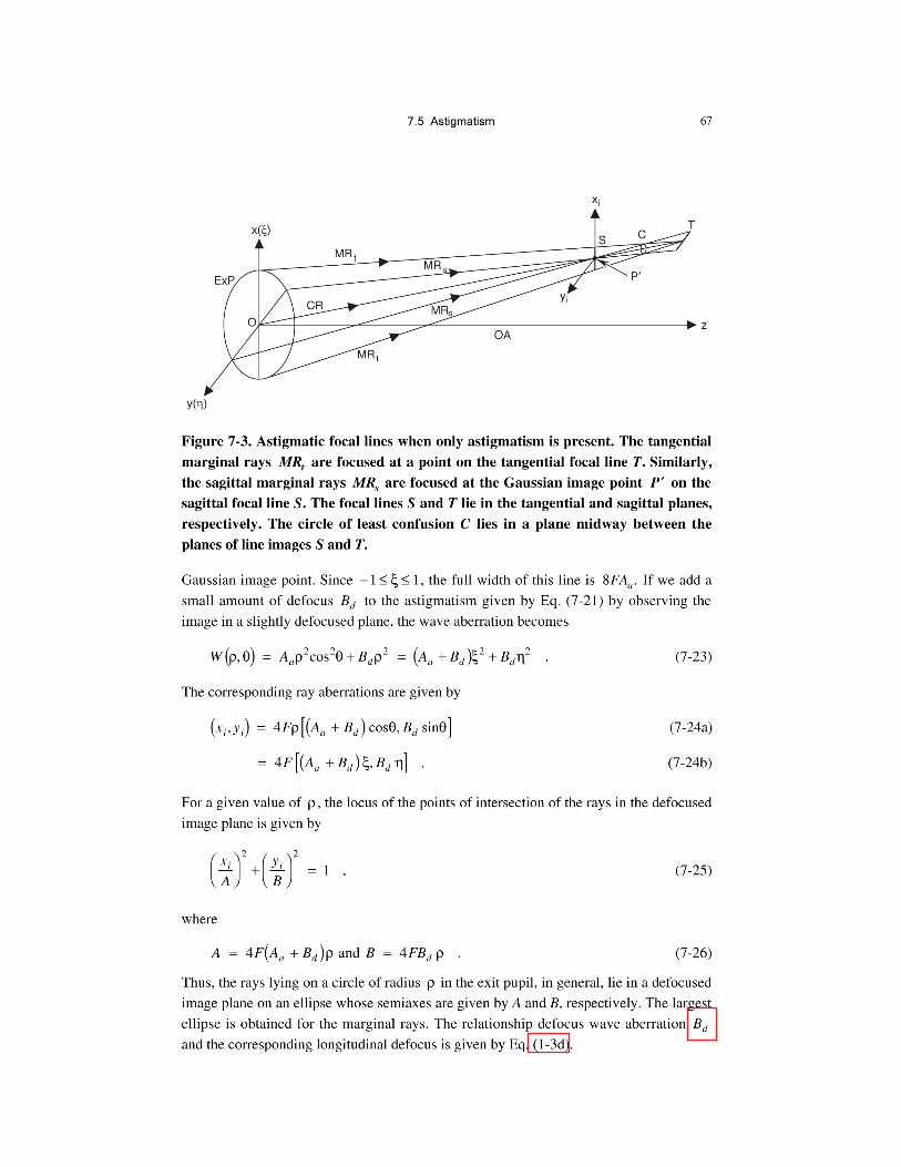
7.5 ASTIGMATISM

The astigmatism wave aberration is given by

W A Aa ar q r q x, .( ) = =2 2 2cos (7-21)

The corresponding ray aberrations are given by

x y F A F Ai i a a, , , .( ) = ( ) = ( )4 0 4 0r q xcos (7-22)

The point of intersection of a ray with the Gaussian image plane depends only on its xcoordinate in the exit pupil. Thus, as indicated in Figure 7-3, all the rays transmitted by

the exit pupil intersect the Gaussian image plane on a line along the x axis centered on the

(7-17)

68 RAY SPOT SIZES AND DIAGRAMS

We note that if Bd = 0, the ellipse reduces to a line of full width of 8FAa along the x

axis. Thus, as discussed above, the image in the Gaussian image plane is a line S along

the x axis centered on the Gaussian image point. If, however, B Ad a= - , corresponding

to D = 8 2F Aa , then the ellipse reduces to a line T along the y axis. The full width of this

line image is the same as that of the line image S. The line image along the x axis is called

the sagittal (or radial) image and lies in the tangential (or meridional) plane zx,

containing the point object (which lies along the x axis in the object plane) and the optical

axis. Similarly, the line image T along the y axis is called the tangential image and lies in

the sagittal plane yz. The distance 8 2F Aa between the two line images is called

longitudinal astigmatism. The two line images are called the astigmatic focal lines.

If B Ad a= - 2 , corresponding to D = 4 2F Aa , the ellipse reduces to a circle of

maximum diameter of 4FAa ,which is half the full width of the two line images. Since

this circle is the smallest of all the possible images, Gaussian or defocused, it is called the

circle of least (astigmatic) confusion. The spot sigma is minimum and equal to 2FAa in

this plane.

Since A ha ~ ¢2, the width of the line images of a point object increases quadratically

with the height h' of the Gaussian image point. Similarly, longitudinal astigmatism

8 2F Aa increases as ¢h 2 Thus, if we consider a line object, its sagittal image will also be

a line, which is slightly longer (by an amount 8FAa ) than but coincident with its

Gaussian image. However, its tangential image will be parabolic with a vertex radius of

curvature of ¢h F Aa2 216 or 1 4 2R aa . Similarly, the sagittal image of a planar object

will be planar, but its tangential image will be paraboloidal. Note that longitudinal

astigmatism corresponding to a Gaussian image at a height h' represents the sag of the

tangential image surface at that height.

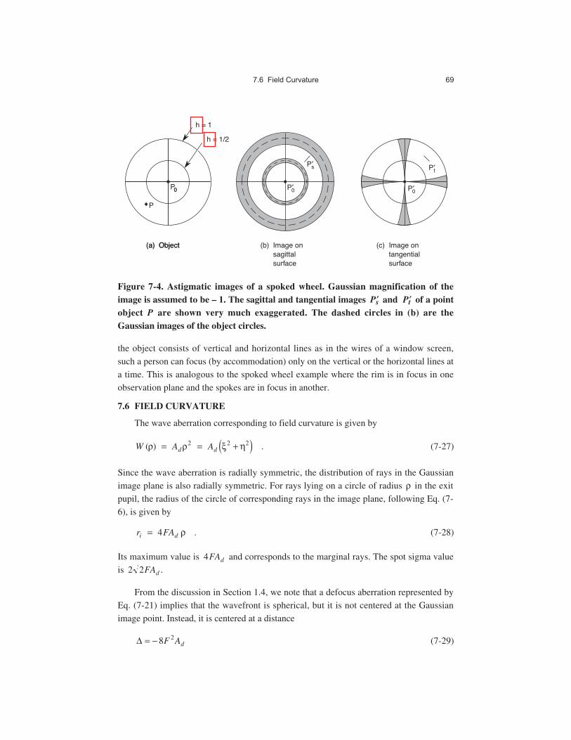
Figure 7-4 illustrates the effect of astigmatism and field curvature on the image of a

spoked wheel where the images formed on the sagittal and tangential surfaces are shown.

A magnification of - 1 is assumed in the figure. As discussed earlier, a point object P is

imaged as a sagittal or radial line ¢Ps on the sagittal surface and as a tangential line ¢Pt on

the tangential surface. Each point on the object is imaged in this manner, so that the

sagittal image consists of sharp radial lines and diffuse circles while the tangential image

consists of sharp circles and diffuse radial lines. If the object contains lines that are

neither radial nor tangential, they will not be sharply imaged on any surface.

It should be understood that the astigmatism discussed here is for a system that is

rotationally symmetric about its optical axis, and its value reduces to zero for an axial

point object. It is different from the astigmatism of the eye, which is caused by one or

more of its refracting surfaces, usually the cornea, that is curved more in one plane than

another. The refracting surface that is normally spherical acquires a small cylindrical

component, i.e., it becomes toric. Such a surface forms a line image of a point object even

when it lies on its axis. Hence, a person afflicted with astigmatism sees points as lines. If

8 2F A2a ,= 8

4 2F A2a ,

(a)

P

P0

��= 1

Object

��= 1/2

(a)

0

Object (b)

P¢s

P¢0

(c) Image ontangentialsurface

P¢t

P¢0

Image onsagittalsurface

Figure 7-4. Astigmatic images of a spoked wheel. Gaussian magnification of theimage is assumed to be – 1. The sagittal and tangential images ¢Ps and ¢Pt of a pointobject P are shown very much exaggerated. The dashed circles in (b) are theGaussian images of the object circles.

the object consists of vertical and horizontal lines as in the wires of a window screen,

such a person can focus (by accommodation) only on the vertical or the horizontal lines at

a time. This is analogous to the spoked wheel example where the rim is in focus in one

observation plane and the spokes are in focus in another.

7.6 FIELD CURVATURE

The wave aberration corresponding to field curvature is given by

W A Ad d( ) .r r x h= = +( )2 2 2 (7-27)

Since the wave aberration is radially symmetric, the distribution of rays in the Gaussian

image plane is also radially symmetric. For rays lying on a circle of radius r in the exit

pupil, the radius of the circle of corresponding rays in the image plane, following Eq. (7-

6), is given by

r FAi d= 4 r . (7-28)

Its maximum value is 4FAd and corresponds to the marginal rays. The spot sigma value

is 2 2FAd .

From the discussion in Section 1.4, we note that a defocus aberration represented by

Eq. (7-21) implies that the wavefront is spherical, but it is not centered at the Gaussian

image point. Instead, it is centered at a distance

D = - 8 2F Ad (7-29)

���������� ���� � ��

100 SYSTEMS WITH CIRCULAR PUPILS

8.5 OPTICAL TRANSFER FUNCTION (OTF)

Since the diffraction image of an incoherent object is given by the convolution of its

Gaussian image and the system PSF, a Fourier transform of this relationship shows that

the spatial frequency spectrum of the diffraction image is given by the product of the

spectrum of the Gaussian image and the optical transfer function (OTF) of the system,

where the OTF is equal to the Fourier transform of the PSF.1-3 Because of the relationship

of Eq. (8-1) between the PSF and the pupil function of the system, the OTF is also given

by the autocorrelation of the pupil function. Thus, the OTF of a system can be obtained

from its pupil function without having to calculate its PSF. In this section, we introduce

the concept of OTF and discuss its physical significance. We also discuss how it is

affected by aberrations and how it relates to the Strehl ratio. Also given is an expression

for the aberration-free OTF of a system with a circular pupil. Contrast reversal is also

illustrated, in which bright regions of certain bands of spatial frequencies in the object are

imaged as dark, and dark regions are imaged as bright.

8.5.1 OTF and Its Physical Significance

The OTF of an incoherent imaging system is given by the Fourier transform of its

PSF according to

tr r r r rv PSF r i v r d ri i i i i( ) = ( ) p( )Ú ◊exp 2 (8-33)

where rv vi i= ( ), f is a 2D spatial frequency vector in the image plane,

rr Fri i= ( )l q, is

the position vector of a point in this plane, and the PSF is given by Eq. (8-1) with P = 1.

In what follows, we assume that the Fresnel number of the system is large so that the

defocus tolerance dictates that z ~ R. However, if this is not the case, then we simply

replace R by z in the following discussion. As mentioned above, because of Eq. (8-1)

relating the PSF and the pupil function, the OTF may also be written as the

autocorrelation of the pupil function, i.e.,

t lr r r r rv S P r P r R v d ri p p p i p( ) = ( ) * -( )Ú-1 , (8-34)

where

P r i r r ap p p

r r r( ) = ( )[ ] £ £exp ,F 0 (8-35)

= 0 , otherwise

is the pupil function. Here, rr ap = ( )r q, is the position vector of a point in the plane of the

exit pupil. The integration in Eq. (8-34) is carried out across the region of overlap of two

pupils centered at rrp = 0 and the other at

r rr Rvp i= l . The asterisk in Eq. (8-34) indicates

a complex conjugate.

The OTF depends on the wavelength in two ways. First, the dependence of the phase

aberration on it is evident. Second, it enters in the displacement of the pupil. It has the

implication that for a longer wavelength the displacement approaches the diameter of the

(8-34)

901References

References

1. V. N. Mahajan, Optical Imaging and Aberrations, Part II: Wave DiffractionOptics (SPIE Press, Bellingham, WA, Second Edition 2011).

2. M. Born and E. Wolf, Principles of Optics, 7th ed. (Cambridge University Press,New York, 1999).

3. J. W. Goodman, Introduction to Fourier Optics, 2nd ed. (McGraw-Hill, NewYork, 1996).

4. G. B. Airy, “On the diffraction of an object-glass with circular aperture,” Trans.Camb. Phil. Soc. 5, 283–291 (1835).

5. V. N. Mahajan, “Axial irradiance and optimum focusing of laser beams,” Appl.Opt. 22, 3042–3053 (1983).

6. A. Maréchal, “Etude des effets combines de la diffraction et des aberrationsgeometriques sur 1'image d'un point lumineux,” Rev. d'Opt. 26, 257–277 (1947).

7. B. R. A. Nijboer, “The diffraction theory of aberrations,” Ph.D. thesis (Universityof Groningen, Groningen, The Netherlands, 1942), p. 17.

8. V N. Mahajan, “Strehl ratio for primary aberrations in terms of their aberrationvariance,” J. Opt. Soc. Am. 73, 860–861 (1983).

9. V N. Mahajan, “Strehl ratio for primary aberrations: some analytical results forcircular and annular pupils,” J. Opt. Soc. Am. 72, 1258–1266 (1982).

10. V N. Mahajan, “Line of sight of an aberrated optical system,” J. Opt. Soc. Am. A2, 833–846 (1985).

11. W. B. King, “Dependence of the Strehl ratio on the magnitude of the variance ofthe wave aberration,” J. Opt. Soc. Am. 58, 655–661 (1968).

12. Lord Rayleigh, “Investigations in optics, with special reference to thespectroscope,” Phil. Mag. (5) 8, 403–411 (1879); also his Scientific Papers, Vol. 1(Dover, New York, 1964), p. 432.

13. V. N. Mahajan, “Symmetry properties of aberrated point-spread functions,” J.Opt. Soc. Am. A 11, 1993–2003 (1994).

14. V N. Mahajan, “Aberrated point spread functions for rotationally symmetricaberrations,” Appl. Opt. 22, 3035–3041 (1983).

15. S. Szapiel, “Aberration-variance-based formula for calculating point-spreadfunctions: rotationally symmetric aberrations,” Appl. Opt. 25, 244–251 (1986).

16. H. H. Hopkins, “The aberration permissible in optical systems,” Proc. Phys. Soc.(London) B52, 449–470 (1957).

Part II:

126 SYSTEMS WITH ANNULAR AND GAUSSIAN PUPILS

deviation of the corresponding polynomial term. The variance of the aberration function

is given by

s r q r qF F F2 2 2= ( ) - ( ), ; , ;� �

= Â Â -=

•

=n m

n

nmc c0 0

2002

= Â Â=

•

=n m

n

nmc1 0

2 . (9-19)

The Zernike annular radial polynomials for n £ 6 are listed in Table 9-3. The number

of Zernike (or orthogonal) aberration terms in the expansion of an aberration function

through a certain order n is the same as in the case of circle polynomials. The balanced

aberrations given in Table 9-2 can be identified with the annular polynomials. Thus the

polynomials Z22, Z3

1 , and Z40 represent balanced astigmatism, coma, and spherical

aberration. From the form of the annular polynomial R22 2r q; cos�( ) , it is evident that the

balancing defocus in the case of astigmatism is independent of the value of �. The

annular polynomials are unique in that they are the only polynomials that are orthogonal

across an annular pupil and represent balanced aberrations for such a pupil, just as the

circle polynomials discussed in Section 8.3.7 are unique for the circular pupils. Whereas

the aberration function for a rotationally symmetric system consists of polynomials

varying as cos mq , an aberration function representing fabrication errors will generally

consist of polynomials varying as sin mq as well. The single-index annular polynomials

Z j r q, ; �( ) can be constructed in the same manner as the corresponding single index circle

polynomials Z j r q,( ) discussed in Section 8.3.7.

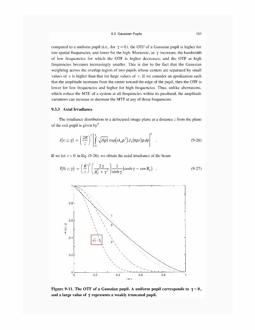
9.3 GAUSSIAN PUPILS

So far we have considered optical systems that have uniform amplitude across their

exit pupils. Now we consider systems with exit pupils having nonuniform amplitude

across them in the form of a Gaussian.5,6 Such pupils are often referred to as Gaussian

pupils. The Gaussian amplitude may, for example, be obtained by placing a filter with

Gaussian transmission at the pupil. A system with a nonuniform amplitude across its

pupil is called an apodized system. The motivation for apodizing a system is to reduce the

values of the secondary maxima of its PSF relative to the value of the principal

maximum. The discussion given here applies equally well to the propagation of Gaussian

laser beams. For a Gaussian pupil transmitting the same total power as a circular pupil

with uniform transmission, the central value of the PSF is smaller and the tolerance for an

aberration is higher.

9.3.1 Aberration-Free PSF

The Gaussian amplitude may be written

A Ar g r( ) = -( )02exp , (9-20)

S5,6n.5

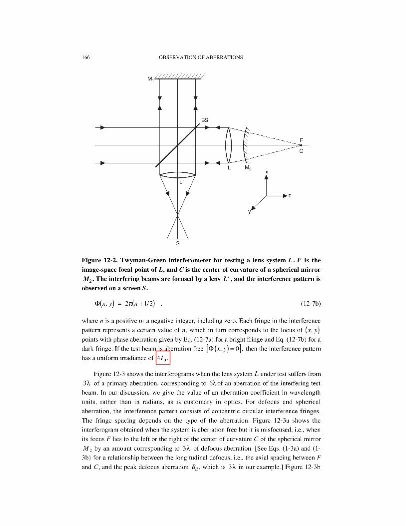
168 OBSERVATION OF ABERRATIONS

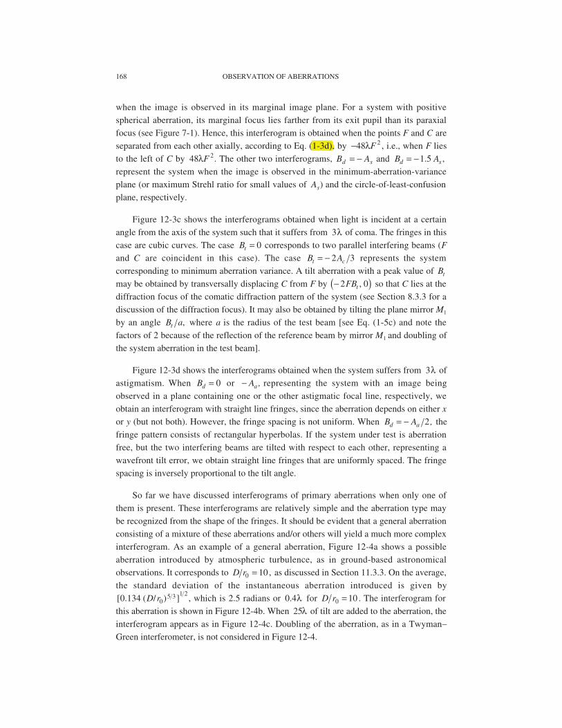
when the image is observed in its marginal image plane. For a system with positive

spherical aberration, its marginal focus lies farther from its exit pupil than its paraxial

focus (see Figure 7-1). Hence, this interferogram is obtained when the points F and C are

separated from each other axially, according to Eq. (1-3d), by -48 2lF , i.e., when F lies

to the left of C by 48 2lF . The other two interferograms, B Ad s= - and B Ad s= -1 5. ,

represent the system when the image is observed in the minimum-aberration-variance

plane (or maximum Strehl ratio for small values of As) and the circle-of-least-confusion

plane, respectively.

Figure 12-3c shows the interferograms obtained when light is incident at a certain

angle from the axis of the system such that it suffers from 3l of coma. The fringes in this

case are cubic curves. The case Bt = 0 corresponds to two parallel interfering beams (F

and C are coincident in this case). The case B At c= - 2 3 represents the system

corresponding to minimum aberration variance. A tilt aberration with a peak value of Bt

may be obtained by transversally displacing C from F by -( )2 0FBt , so that C lies at the

diffraction focus of the comatic diffraction pattern of the system (see Section 8.3.3 for a

discussion of the diffraction focus). It may also be obtained by tilting the plane mirror M1

by an angle B at , where a is the radius of the test beam [see Eq. (1-5c) and note the

factors of 2 because of the reflection of the reference beam by mirror M1 and doubling of

the system aberration in the test beam].

Figure 12-3d shows the interferograms obtained when the system suffers from 3l of

astigmatism. When Bd = 0 or - Aa , representing the system with an image being

observed in a plane containing one or the other astigmatic focal line, respectively, we

obtain an interferogram with straight line fringes, since the aberration depends on either x

or y (but not both). However, the fringe spacing is not uniform. When B Ad a= - 2 , the

fringe pattern consists of rectangular hyperbolas. If the system under test is aberration

free, but the two interfering beams are tilted with respect to each other, representing a

wavefront tilt error, we obtain straight line fringes that are uniformly spaced. The fringe

spacing is inversely proportional to the tilt angle.

So far we have discussed interferograms of primary aberrations when only one of

them is present. These interferograms are relatively simple and the aberration type may

be recognized from the shape of the fringes. It should be evident that a general aberration

consisting of a mixture of these aberrations and/or others will yield a much more complex

interferogram. As an example of a general aberration, Figure 12-4a shows a possible

aberration introduced by atmospheric turbulence, as in ground-based astronomical

observations. It corresponds to D r0 10= , as discussed in Section 11.3.3. On the average,

the standard deviation of the instantaneous aberration introduced is given by

[ . ( / ) ]0 134 05 3 1 2

D r , which is 2.5 radians or 0 4. l for D r0 10= . The interferogram for

this aberration is shown in Figure 12-4b. When 25l of tilt are added to the aberration, the

interferogram appears as in Figure 12-4c. Doubling of the aberration, as in a Twyman–

Green interferometer, is not considered in Figure 12-4.

(1-3d),