Embed Size (px)
Citation preview

Accurate Fault Location in TransmissionNetworks Using Modeling, Simulation
and Limited Field Recorded Data
Final Project Report
Power Systems Engineering Research Center
A National Science FoundationIndustry/University Cooperative Research Center
since 1996
PSERC

AcM
Power Systems Engineering Research Center
curate Fault Location in Transmission Networks Using odeling, Simulation and Limited Field Recorded Data
Final Project Report
Project Team
Mladen Kezunovic, Project Leader Shanshan Luo, Zjiad Galijasevic, Dragan Ristanovic
Texas A&M University
PSERC Publication 02-44
November 2002

Information about this project For information about this project contact: Mladen Kezunovic, Ph.D., P.E. Eugene E. Webb Professor Texas A&M University Department of Electrical Engineering College Station, TX 77845-3128 Tel. 979-845-7509 Fax. 979-845-9887 Email. [email protected] Power Systems Engineering Research Center This is a project report from the Power Systems Engineering Research Center (PSERC). PSERC is a multi-university Center conducting research on challenges facing a restructuring electric power industry and educating the next generation of power engineers. More information about PSERC can be found at the Center’s website: http://www.pserc.wisc.edu. For additional information, contact: Power Systems Engineering Research Center Cornell University 428 Phillips Hall Ithaca, New York 14853 Phone: 607-255-5601 Fax: 607-255-8871 Notice Concerning Copyright Material PSERC members are given permission to copy without fee all or part of this publication for internal use if appropriate attribution is given to this document as the source material. This report is available for downloading from the PSERC website.
2002 Texas A&M University. All rights reserved.

ACKNOWLEDGEMENTS The work described in this report was sponsored by the Power Systems Engineering Research Center (PSERC). We express our appreciation for the support provided by PSERC’s industrial members and by the National Science Foundation under grant NSF EEC 0002917 received under the Industry/University Cooperative Research Center program. Particular thanks go to ABB, Entergy Services, Mitsubishi ITA, Oncor Group, CenterPoint Energy and Tennessee Valley Authority for their involvement in the project. Also, special thanks are due to Don R. Sevcik from CenterPoint Energy for his valued comments and guidance.

ii
EXECUTIVE SUMMARY Fault location on transmission lines is a very important application aimed at identifying the exact location of the fault and repairing the fault conditions with a goal of restoring the system as quickly as possible. With transmission lines equipped with digital relays at either ends or dedicated fault locators, the task of locating faults is rather simple. If most of the relays in the system are electromechanical or if transmission lines have multiple taps, the required measurements are not available and locating faults accurately is very difficult.
Fortunately, recording devices such as digital fault recorders (DFRs) are installed at some substations for fault monitoring and analysis. When a fault occurs, DFRs are triggered and will record pre-selected quantities. Generally, the recordings are available only at a few locations due to the number of installed DFRs being typically much lower than the number of substations in a given system. Alternatively, the recording devices may be extensively installed at substations in the system, but every installed recording device may not be triggered by a fault. In either case, when a fault occurs, only sparsely-located measurements are obtained. This type of data is denoted as “sparse data”. Under this situation, many proposed algorithms for estimating fault location based on DFR measurements may fail to produce accurate results.
This project is aimed at developing accurate fault location algorithms for situations where only sparse field data is available. The basic concept of matching the recorded and simulated waveforms to determine the most probable fault location is utilized. The recorded waveforms are captured using DFRs while the simulated waveforms are produced running a short circuit program using an accurate model of the power system. This study investigated the feasibility of the new fault location algorithm and proposed possible improvements to it.
To determine the degree of matching between recorded and simulated waveforms, the during-fault phasor is used to calculate the fitness value. The procedure of finding the best-matched simulation waveform is an optimization problem. There are many approaches for solving an optimization problem. In this study, a genetic algorithm is used. For enabling the usage of the fault location software developed in this study, data requirements are specified. The PSS/E model and DFR files are necessary to run the software. PSS/E software is commercial software used to calculate the power flow and carry out short circuit studies. Fifteen fault cases provided by CenterPoint Energy were used for testing the algorithm thoroughly using several different versions of the PSS/E model.
The performance of the fault location algorithm and software was analyzed. The results of the analysis suggest that many factors may affect the accuracy of the proposed fault location algorithm. The most important factor is the power system model accuracy. The model may not reflect the real system operation condition when a fault occurs. Therefore, the static system model should be updated to reflect the real condition. Other factors affecting the accuracy of the fault location estimate include exact phasor calculation, synchronization, determination of the fault inception, selection of branch candidates, and genetic algorithm convergence. Based on the analysis, several improvements were made. The final test results show that the genetic algorithm is very promising in its ability to accurately estimate the fault location.

iii
TABLE OF CONTENTS
1 INTRODUCTION .................................................................................................................... 1
2 SCHEME OF NEW FAULT LOCATION APPROACH..................................................... 3 2.1 Introduction......................................................................................................................... 3 2.2 Sparse data .......................................................................................................................... 3 2.3 Waveform matching............................................................................................................ 4 2.4 Criteria for determining the matching degree..................................................................... 5 2.5 Simulation results................................................................................................................ 6 2.6 Optimal approach................................................................................................................ 7 2.7 Genetic algorithm overview................................................................................................ 8 2.8 Conclusion ........................................................................................................................ 10
3 IMPLEMENTATION OF THE GENETIC ALGORITHM.............................................. 11 3.1 Introduction....................................................................................................................... 11 3.2 Solution representation ..................................................................................................... 11
3.2.1 Encoding................................................................................................................... 11 3.2.2 Decoding................................................................................................................... 11
3.3 Mapping objective function to fitness function ................................................................ 12 3.4 Fitness scaling................................................................................................................... 12 3.5 Multi-point crossover........................................................................................................ 14 3.6 Convergence ..................................................................................................................... 16
3.6.1 Maximum fitness value behavior ............................................................................. 17 3.6.2 Using a refined genetic algorithm ............................................................................ 20 3.6.3 Conclusions regarding convergence......................................................................... 21
3.7 Conclusions....................................................................................................................... 22
4 IMPLEMENTATION OF THE FAULT LOCATION ALGORITHM............................ 23 4.1 Introduction....................................................................................................................... 23 4.2 Architecture....................................................................................................................... 23 4.3 Obtaining phasors ............................................................................................................. 26 4.4 Fault cycles ....................................................................................................................... 29 4.5 Signal processing .............................................................................................................. 31
4.5.1 DC offset component................................................................................................ 31 4.5.2 High frequency noise................................................................................................ 33
4.6 Synchronizing the phasors obtained from DFR recordings.............................................. 34 4.7 Processing the static model............................................................................................... 35
4.7.1 Determining the topology......................................................................................... 36 4.7.2 Tuning static system................................................................................................. 38
4.8 Conclusions....................................................................................................................... 44

iv
TABLE OF CONTENTS (continued)
5 TEST RESULTS..................................................................................................................... 45 5.1 Introduction....................................................................................................................... 45 5.2 Example I .......................................................................................................................... 45
5.2.1 Event Data ................................................................................................................ 45 5.2.2 Diagram .................................................................................................................... 45 5.2.3 Sensitivity Study....................................................................................................... 46
5.3 Example II......................................................................................................................... 46 5.3.1 Event Data ................................................................................................................ 46 5.3.2 Diagram .................................................................................................................... 47 5.3.3 Sensitivity study ....................................................................................................... 47
5.4 Summary of results ........................................................................................................... 48 5.5 Conclusions....................................................................................................................... 48
6 CONCLUSIONS..................................................................................................................... 49
7 REFERENCES ....................................................................................................................... 50

v
LIST OF FIGURES
Fig. 1 The sample system for illustrating data scarcity ................................................................. 4 Fig. 2 The fitness surface for an A-G fault .................................................................................... 7 Fig. 3 A generation of a simple genetic algorithm......................................................................... 8 Fig. 4 Simple reproduction allocates offspring strings using a roulette wheel with slots sized
according to fitness ............................................................................................................. 9 Fig. 5 Single parameter and multiple parameter encoding .......................................................... 12 Fig. 6 Scaled Fitness .................................................................................................................... 13 Fig. 7 The unexpected scaled fitness ........................................................................................... 14 Fig. 8 Maximum fitness value for case III, resistance range 0-0.8 p.u. ....................................... 17 Fig. 9 Maximum fitness value for case III, resistance range 0-0.4 p.u. ....................................... 17 Fig. 10 Maximum and average fitness value for Case IX............................................................ 18 Fig. 11 Test results obtained from Case IX; two curves are obtained by using
the same input file (caseXI-1.tot)...................................................................................... 19 Fig. 12 Case IX (setting the “out_iteration” to 9, “in_iteration” to 10)....................................... 20 Fig. 13 Fitness value for case IX, using refined GA, Pc (0)=0.9, Pm (0)=0.01............................ 21 Fig. 14 Architecture of fault location software............................................................................ 24 Fig. 15 The selection of fault location algorithms ....................................................................... 25 Fig. 16 Phasors obtained from the recorded waveforms.............................................................. 26 Fig. 17 Three phase voltage waveforms ...................................................................................... 27 Fig. 18 RMS values of the voltage signals .................................................................................. 27 Fig. 19 The phase angle shift of the voltage signals .................................................................... 29 Fig. 20 Case IV: current waveforms on Exxon Ckt.83 in Cedar Bayou...................................... 30 Fig. 21 Current waveforms on Dupont-Deer Pk Ckt 85 in Cedar Bayou................................... 31 Fig. 22 Case IX: current waveforms on Holman Ckt. 44 (138KV)............................................. 32 Fig. 23 Case XII: current waveforms on TP&L Jewett Ckt. 98 from Limestone (345 KV) ....... 33 Fig. 24 Case I, current waveform of section 4110-4111.............................................................. 34 Fig. 25 The relationship between the phasors obtained by load flow study and
by recorded waveforms..................................................................................................... 35 Fig. 26 A sample system.............................................................................................................. 36 Fig. 27 The flowchart of tuning static system model................................................................... 40 Fig. 28 The flowchart for local tuning of the static system model .............................................. 43 Fig. 29 One-Line Diagram of section of CenterPoint Energy transmission system.................... 45 Fig. 30 One-Line Diagram of section of CenterPoint Energy transmission system.................... 47

1 INTRODUCTION How to find a fault location in a transmission network is an important problem because identifying an accurate fault location can facilitate rapidly repairing any damage and restoring the faulty transmission line to service. It is especially critical for the permanent fault in a large-scale transmission system. If a fault location cannot be identified quickly and, as a result, the line outage time is prolonged during a period of peak load, there will be severe economic loss and reliability issues.
A lot of effort have been made on the topic and several solutions were proposed. However, they cannot be applied in all circumstances. Basically there are the following solution classes.
1. Methods based on using expert’s knowledge and combining the recordings to locate a fault.
In references [1] and [2], expert systems utilize both the binary quantities (relay and breaker status) and analog quantities (voltage and current measurements). The binary information is used to estimate the fault section, such as a bus or a line. The analog quantities are used to further pinpoint a fault location.
2. Calculating the line impedance to locate a fault.
Various one-end, two-end or three-end algorithms utilizing the voltage and current quantities for estimating the fault location have been proposed[3][4][5][6][7]. The one-end algorithm is the simplest and does not require the communication of data between the monitoring devices located at different ends of the same transmission line. However, the fault resistance and remote-in feed may adversely affect its accuracy. For the special case where each end of parallel transmission lines is located at the same tower and two DFRs are installed at only one end (common bus) of parallel lines, one-end of the algorithm can give highly accurate results despite the fault resistance impact [8]. Two-end and three-end algorithms are essentially independent of the fault resistance and yield quite accurate estimates. While synchronized sampling may obtain better results than unsynchronized sampling, it needs additional system requirements like Phasor Measurement Units for interfacing the timing signals for sampling synchronization from the GPS [9].
3. Methods based on measurement of the fault generated traveling wave component [10][11].
The methods in this class make use of traveling waves generated by faults for estimating a fault location. The main advantages of such algorithms are improved

2
accuracy and insensitivity to series compensation capacitors. There are drawbacks. Conventional current transformers cannot satisfy the requirements of accuracy and sampling rates; therefore, the capacitor voltage transforms are utilized for obtaining the transform waveform. Another problem is the situation where traveling waves are not produced when a fault occurs at a voltage inception angle close to zero. Finally, there can be a problem in distinguishing between traveling waves reflected from the fault and from the remote end of the line.
It has been demonstrated that the existing algorithms are only suitable for specific cases, and there is still no satisfactory solution for every system. For example, in the CenterPoint Energy transmission system, only recorded data at limited substation locations are available. When a fault occurs in such systems, only several (two or three) DFRs may be triggered. The data obtained from triggered DFRs is sparse. Under this situation, there is not enough measurements to locate a fault using the methods mentioned above. A new fault location approach is required in such systems. In the next three sections, the scheme and implementation of a new approach using waveform matching and simulation are presented and corresponding results are shown in the subsequent section.

3
2 SCHEME OF NEW FAULT LOCATION APPROACH
2.1 Introduction
This chapter presents an outline of the proposed fault location approach. Considering that the approach uses sparse data (that is, limited amounts of field data) to locate a fault, the first section presents the concept of sparse data. Then, the scheme of waveform matching and matching criteria are stated. Simulation results are shown subsequently. At the end of the chapter, the optimal approach and selected genetic algorithm are discussed.
2.2 Sparse data
Sparse data refers to the data obtained from recording devices sparsely located at substations in a power system network. Examples of recording devices may include digital fault recorders (DFRs), digital relays, or other intelligent electronic devices (IEDs). The data captured by recording devices may include analog quantities, such as voltages and currents, as well as digital quantities such as breaker and relay operation status. Both analog and digital quantities may be useful for locating the fault. Digital quantities can be used to estimate the fault section and analog signals can further be used to calculate the exact fault location.
The sparse data may include two possible cases. In the first case, many systems, recording device may not be installed at every substation or bus for monitoring purposes. It is common that only a small number of the buses or substations in the system have recording devices installed. In the second case, the recording devices may be extensively installed at the substations in the system, but every recording device installed may not be triggered by a fault. It is possible that only limited recording devices may be triggered under certain fault conditions. Based on some fault cases provided by CenterPoint Energy, the minimum number of triggered DFRs is one, the largest number of triggered DFRs is three. In either case, when a fault occurs on a system, only sparsely located measurements are obtained from the limited number of triggered recording devices. This type of data is denoted as “sparse data”.
Fig. 1 illustrates the concept of sparse data. The system represents a part of the 138 kV CenterPoint Energy transmission system. While the system part has a total of 19 buses, DFRs are installed at three buses only. Clearly, the system is sparsely monitored. When a fault occurs on the line between bus 11 and bus 12, the DFRs located at buses 1, 3, or 16 may be triggered to record the specified quantities during the fault. In certain cases some of the DFRs at buses 1, 3, 16 may not be triggered. Then even fewer measurements will become available for locating the fault. The data obtained in these cases may be interpreted as “sparse data”.
In such a system, the fault may be several buses away from the DFR locations. Therefore, none of the common algorithms (such as one-end, two-end and three-end and so on) is applicable for

4
locating the faults. To solve this problem, the waveform matching approach is proposed as follows.
Fig. 1 The sample system for illustrating data scarcity
2.3 Waveform matching
In the waveform matching approach, the model of the power system is utilized to carry out simulation studies. The matching is made between the voltage and current waveforms obtained by recording devices and those generated in simulation studies. The fault location is searched through the system by utilizing an iterative search process. The search process consists of the following steps.
First, an initial fault location is assumed and asserted in the model. Second, the simulation studies are configured according to the specified fault. Third, the simulation studies corresponding to the specified fault are carried out utilizing appropriate simulation tools. Fourth, simulated waveforms of quantities of interest are obtained. Fifth, the corresponding simulated waveforms are compared with recorded ones, and the matching degree of the simulated and recorded waveforms is evaluated by using appropriate criteria. Sixth, the initial fault location is modified according to certain approaches, and then the process proceeds to the second step and continues. The above steps are iterated until the simulated waveforms that match the best the recorded ones are produced. The fault location will be determined as the one specified in the simulation studies for the case when generating simulated waveforms best match the recorded ones.
To evaluate the matching degree of the simulated and recorded waveforms, two different methods may be employed. The first one is using phasors for matching. The second one is using transients for matching. In the phasor matching based approach, short circuit studies are carried out to obtain phasors under specified fault conditions. Then the phasors are compared with those derived from the recorded waveform. In the transient matching based approach, transient studies

5
are carried out to obtain the transients generated by the specified faults. Then the transients are compared with the corresponding ones extracted from the recorded waveforms.
For the phasor matching, a short circuit model of the system is needed. For transient matching, a transient model of the system is needed. In our work, the short circuit model of PSS/E provided by CenterPoint Energy is used for short circuit studies [12]. In this stage of our work, only the “phasor matching” based approach for fault location is utilized.
In order to obtain the best waveform match, the search range should be extensive enough to cover all possible faulted branches. There are certain difficulties involved in implementing the method. First, it may be time-consuming. The worst situation is to search all branches in the whole power system. Besides this point, the fault resistance has to be considered. Therefore, the search process is two-dimensional. Second, there is no preferred approach for guiding the search process. The engineers have difficulty in knowing where to pose faults in the next iteration step. It is possible to pose faults randomly. The fault may occur far away from the recording device locations in a big system. To determine the possible area for posing faults is challenging.
2.4 Criteria for determining the matching degree
In the phasor matching based approach, phasors generated from simulation studies (i.e., short circuit studies and those obtained from recorded waveforms) are needed. Short circuit studies can usually directly generate the simulation results in the phasor form. An appropriate signal processing technique needs to be applied in order to extract phasors from the recorded waveforms. Fourier transform may be used for this purpose [13][14][15].
In order to determine the matching degree between the simulated and recorded phasor and find the best match, a quantitative criterion for determine the matching degree is necessary. First, the variables should be determined. As mentioned above, to pose a fault in PSS/E, a fault location, fault type and fault resistance should be specified. For fault type, the user provides the information. The parameters that will be varied are fault location and fault resistance. Next, the matching degree can be formulated as follows:
( ) ∑∑==
−+−=iN
kkrkski
Nv
kkrkskvfc IIrVVrRxf
11, &&&& (2.1)
or
( ) ∑∑==
−+−=iN
kkrkski
Nv
kkrkskvfc IIrVVrRxf
11, &&&& (2.2)
where
( )fc Rxf , : the defined cost function when using phasor angle and magnitude or magnitude only for matching
x : the fault location

6
fR : the fault resistance
kvr and kir : the weights for the errors of the voltage and current measurements respectively
ksV and krV : the during-fault voltage phasors obtained from the short circuit simulation studies and recorded waveforms respectively
ksI and krI : the during-fault current phasors obtained from the short circuit studies and recorded waveforms respectively
k : the index of the voltage or current phasors match
vN and iN : the total number of voltage and current phasors to be matched respectively.
The cost function ( )fc Rxf , equals to zero theoretically when the phasors obtained from simulation studies exactly match those obtained from recorded waveforms. Therefore, for practical purpose, the best fault location estimate would be the one that minimizes the cost function. An appropriate optimization procedure needs to be selected to solve the minimized problem. Equations 2.1 and 2.2 can be converted into the maximum problem shown as follows,
( ) ( )fcff RxfRxf ,, −= (2.3)
where ( )ff Rxf , represents the fitness function when using phasor or magnitude for matching.
2.5 Simulation results
To investigate the nature of the fitness function, various simulation studies have been carried out to obtain the fitness value versus the fault location and resistance using the sample power system shown in Fig. 1. The fitness value is obtained by specifying the faults with varying fault resistance on each line throughout the system, running simulations, and applying equations (2.2) and (2.3). When posing faults, the fault location changes in steps of 4 miles and the fault resistance in steps of 0.02 p.u. For each fault location and fault resistance, a corresponding fitness value can be obtained. To plot the fitness value versus the fault location and fault resistance, the value of the fault location needs to be defined.
Firstly, the search sequence for all lines in the system should be defined. For example, suppose we pose faults in the following sequence: 1-2, 2-3, 3-4, 4-5, 3-6, 6-7, 7-8, 8-9, 3-10, 10-11, 11-12, 12-13, 13-14, 14-15, 15-16, 3-17, 17-18, 18-19 for the line sequence shown in Fig. 1. Bus 1 is defined as the initial bus for line 1, bus 2 is defined as the initial bus for line 2, and finally the bus 18 is defined as the initial bus for the last line. The fault location is defined as the distance of the fault from the initial bus. When the fault location is determined to be at zero miles, the posed fault location is situated at bus 1. The next fault location is changed based on preset step selected to be 4 miles. If the distance is smaller than the first line (1-2) length, the posed fault is located on the first line from the bus 1. Otherwise, the distance is compared with the sum of the first line

7
(1-2) and the second line (2-3) length. If it is smaller, then the posed fault location is selected on the second line 4 miles (the first line length) away from bus 2.
Now suppose we assume that a phase A to ground fault with fault resistance 0.1 p.u. occurs on the line between buses 13 and 12, and is located 9.1 miles away from bus 13. The fault location is the distance from bus 1 to the fault point and it is obtained by adding those lines’ length, which contains lines 1-2, 2-3, 3-4, 4-5, 3-6, 6-7, 7-8, 8-9, 3-10, 10-11, 11-12, and the distance from bus 12 to the fault point. Therefore, the fault location would be at 312.7 miles according to the above definition. If the recorded data are only available at bus 1, the fitness value versus the fault location and fault resistance for this specific fault can be obtained as depicted in Fig. 2.
In Fig. 2 the maximum fitness value occurs at point (312.7, 0.1), which is the optimal solution for the phase A to ground fault. It is noted that the surface contains some local maximum and saddles. The surface is not regular.
Fig. 2 The fitness surface for an A-G fault
2.6 Optimal approach
To obtain the maximum fitness value and its corresponding fault location and fault resistance, the same approach as described in section 2.5 is used to search whole network and draw the fitness value surface, then pick the optimal solution. The approach is effective. However, it is time consuming and hence impractical for some large, complex power systems.
Many optimization approaches have been applied in the power system field. Most of them are utilized to solve the economic dispatch, maintenance scheduling, fuel resource scheduling, unit commitment and load dispatch for optimal power flow. Basically, the current literature identifies three main types of search methods: calculus-based, enumerative and random. The calculus-based methods seek a local extreme by solving the usually nonlinear set of equations resulting from setting the gradient of the objective function equal to zero or seeking local optima by selecting an initial point and moving in a direction related to the local gradient. However, as seen

8
in Fig. 2, the fitness surface is not regular, and contains saddle points and local maximum points. Simulation studies show similar characteristics for other types of faults. Therefore, it is rather difficult to use the first method to find the global maximum point. The enumerative schemes have been considered in many shapes and sizes. The idea is fairly straightforward: within a finite search space or a discrete infinite search space, the search algorithm starts looking at objective function values at every point in the space, one at a time. The method is simple; however, it lacks efficiency.
Random search algorithms have achieved increasing popularity because of the shortcoming of calculus-based and enumerative schemes. The genetic algorithm (GA) is an example of a search procedure that uses random choice as a tool to guide a highly exploitative search through a coding of a parameter space. The research shows that the GA based optimization approach is good at finding the globally optimal solution and avoiding the local optima; in other words, it is more robust than conventional search methods. Therefore, the GA is selected as the tool for finding the global optima in our study.
2.7 Genetic algorithm overview
Genetic algorithms (GA) are search and optimization methods based on the mechanics of natural selection and natural genetics. Unlike other traditional “hill-climbing” methods involving iterative changes to a single solution, GA works with a population of solutions that evolves in a manner analogous to natural selection. Candidate solutions to an optimization problem are represented by chromosomes, which, for example, encode the solution parameters as a numeric string. The fitness of each solution is calculated using an evaluation function that measures its worth with respect to the objective and constraint of the optimization problem.
Several simple “genetic” operators create successive “generations” of the population, as illustrated in Fig. 3.
Fig. 3 A generation of a simple genetic algorithm
evaluation
0 1 1 0 … 0 1 1 00 1…String k, evaluation fk
selection
crossover mutation

9
In each generation, solutions are selected stochastically according to their fitness in order to be recombined to form the next generation. Relatively “fit” solutions survive; “unfit” solutions tend to be discarded. A new generation is created by stochastic operators (typically the “crossover”) that swaps parts of binary-encoded solution strings and that changes (or “mutates”) random bits in the strings. Successive generations yield fitter solutions that are approaching the optimal solution to the problem. The details related to the implementation are as follows.
The mechanics of a simple genetic algorithm are surprisingly simple, involving nothing more complex than copying strings and swapping partial strings. A simple genetic algorithm that yields good results in many practical problems is composed of three operators: Reproduction, Crossover and Mutation.
Reproduction is a process in which individual strings are copied according to their objective function values f . In the biological field this function is called the fitness function. Copying strings according to their fitness values means that strings with a higher value have a higher probability of contributing one or more offspring in the next generation. The reproduction operator may be implemented in an algorithmic form in a number of ways. The simplest way is to create a biased roulette wheel. Each string in the current generation will be allocated a slot sized in proportion to its fitness. In the Fig. 4, for each string i in the population, its fitness is evaluated as fi. The appropriate share of the roulette wheel to allot the ith string is obtained as
∑=
N
kk
i
f
f
1
. Thus, those strings with high fitness values are allocated a large share of the wheel,
while those strings with low fitness values are given a relatively small portion of the roulette wheel. To reproduce, we just “spin” the weighted roulette wheel N times (where N is the number of the current population) to yield the reproduction candidate.
∑
=
N
kk
i
f
f
1
Fig. 4 Simple reproduction allocates offspring strings using a roulette wheel with slots sized according to fitness
After reproduction, the crossover may proceed in two steps. First, pairs of the members of the reproduction candidate strings (where the candidate number should be even) are chosen. Second, each pair of strings undergoes crossover as follows: an integer position k along the string is
25%
49.2%

10
selected uniformly at random between 1 and the string length less one [1, l-1] (where l is the bit number of the string). Exchanging the partial string of the two strings between positions k+1 and l inclusively creates two new strings. The probability that the crossover operator is applied will be denoted by Pc. This process is repeated until all pairs have been covered. Of the three genetic operators, the crossover operator is the most crucial in obtaining the final optimal result because crossover is responsible for mixing the useful information contained in each of the strings of the population in the search; this leads to steadily improving performance.
Next, mutation is applied to the candidate strings after crossover. In the sample GA, mutation is an occasional (with small probability) random alternation of the value of a string position. For the binary coding, the mutation operator is a stochastic bit-wise complement applied with uniform probability Pm The mutation is needed because, even though reproduction and crossover effectively search and recombine high-performance notions, occasionally they may lose some potentially useful genetic material. The mutation operator can be helpful to diversify the search and introduce new strings into the population in order to fully explore the search space. Therefore, it enables the search to overcome local minima. Applying the mutation too frequently may destroy the highly fit strings in the population, which may slow and impede the convergence to a solution. Usually the mutation probability is small; the empirical value is 1.001.0 ≤≤ mP .
The detail operation is as follows. We need to choose a uniform random number [ ]1,0∈r for each bit in a specific string. If mPr ≤ , then the bit is flipped (from 0 to 1 or from 1 to 0); otherwise, the bit remains the same.
After mutation, all candidate strings are copied into the next population. The process is repeated by calculating the fitness of each string, using a roulette wheel method to reproduce, applying the operators of crossover and mutation until a pre-specified convergence criterion is met. Theoretically, when offspring strings in the population are dominated by one individual string, the optimal result is approached. In other words, most of the offspring strings will take on the same value and the strings may not change significantly if iteration continues. The most common convergence criterion is a preset number of generations (that is, iteration number) or a pre-set value for the fitness value.
2.8 Conclusion
Simulations show that the proposed fault location approach using the genetic algorithm should be used to find a global optimum. We conclude that the genetic algorithm is an appropriate approach to find the optimum.
11
3 IMPLEMENTATION OF THE GENETIC ALGORITHM
3.1 Introduction
This chapter mainly presents the details of how the genetic algorithm is implemented in our work. For genetic algorithm convergence, several behaviors of the fitness value are discussed and a proper criterion is suggested.
3.2 Solution representation
Genetic algorithms (GA) were initially developed using binary strings to encode the parameters of an optimization problem. Binary encoding is a standard GA representation that can be employed for many problems; a string of bits can encode integer, real values, sets or whatever is appropriate. However, other representations (such as using strings of integers or floating-point numbers, or using character strings to represent sets) are utilized. Such representations require appropriately designed genetic operators. For our case, the binary encoding representation is selected because the genetic manipulation of binary chromosomes can be done by simple crossover.
3.2.1 Encoding
This step is used to map the parameters of an optimization problem into a binary string of length l. Suppose the variable x ( maxmin xxx ≤≤ ) (assuming the decimal value is positive non-integer number) is to be represented by a binary string of length l. The encoded value x for the variable will be
( )( )
b
l
b xxxx
roundx
−
−−= )
12(
minmax
min (3.1)
where round () gives the nearest integer of the argument, xb and [ ]b represent binary number.
To construct a multiparameter coding, we can simply concatenate on as many single parameter codings as we require. Each coding may have its own sublength and its own xmin and xmax value as represented in Fig. 5.
3.2.2 Decoding
This is to convert the binary string into meaningful decimal parameter employed in the GA. The decoding process is given by

12
minminmax
12)(
xxxx
x bl +−−
= (3.2)
Fig. 5 Single parameter and multiple parameter encoding
3.3 Mapping objective function to fitness function
In many problems (such as the fault location problem mentioned above, discussed section 2.4), the objective is stated as the minimization of the cost function rather than the maximization of some utility or profit function. Even if the problem is naturally stated in a maximization form (formulas in equation 2.3), this alone does not guarantee that the utility function will be nonnegative for all values of the variable x as we require in the fitness function. In GA, a fitness function must be a nonnegative figure of merit [16]. It is necessary to map the objective function to a fitness function form through one or more mappings.
The simplest method is to multiply the cost function by a minus one (see section 2.4). This operation is insufficient because the fitness function must be a nonnegative number. Therefore, the following cost-to-fitness transformation is used:
( ) ( )fc RxfCxf ,max −= (3.3)
where maxC is the maximum ( )fc Rxf , value in the current population.
3.4 Fitness scaling
Ideally, the population size should be as large as possible to enhance the exploration of the search space. The genetic algorithm with a large population can be expensive in terms of computation time, so a small population may be desirable. However, if the population is too small, then the loss of genetic diversity may compromise the search. Genetic diversity is important when the solution space is not topographically smooth. A small population would be more likely to quickly converge on what may be a local optimum; a comparatively fit individual
Single parameter x represented by a binary string of length l=4
0 0 0 0 xmin
……. x maps linearly in between xmin and xmax
1 1 1 1 xmax
Multiparameter coding (10 parameters)

13
in a small starting population will be selected for, and it and its descendants will quickly come to dominate, further limiting genetic diversity. In addition, with the sparse spread of initial points, the global optimum may never be reached before the search converges on a poor local optimum. Even if some local optima are visited, the point may be comparatively unfit, and will not be given an adequate opportunity to reproduce and start hill climbing.
In other words, for genetic algorithm with a small population, the following problem may be encountered. At the beginning of the GA runs, it is common to have a few extraordinary individuals in the population. The extraordinary individuals would take over a significant proportion of the finite population in a single generation, and this may result in premature convergence. On the other hand, near the ending of the procedure for generating GA runs, there may still be significant diversity within the population; however, the population average fitness may be close to the population best fitness. This situation may result in the average and best members getting nearly the same number of copies in future generations. In this case, the survival of the fittest necessary for the improvement becomes random.
To overcome the small population problem, we should have the opportunity to regulate the level of competition among members of the population to achieve the interim and ultimate algorithm performance, as we desire. That is called fitness scaling.
So-called fitness scaling is actually a linear scaling. Let us define the raw fitness f and the scaled fitness f ′ . The relationship between f ′ and f as follows:
bfaf +=′ (3.4)
Fig. 6 Scaled Fitness
The relationship between the raw fitness and scaled fitness is shown in Fig. 6.
The coefficient a and b may be chosen according to the following rules:
The average scaled fitness avgf ′ should be equal to the average raw fitness avgf , because this will insure that each average population member contributes one expected offspring to the next generation.
maxf ′
maxfavgfminf
avgf ′
0
minf ′
SCA
LE
D
Raw fitness

14
To control the number of offspring given to the population member with maximum raw fitness, choose the other scaling relationship to obtain a scaled maximum fitness, avgmult fCf ⋅=′max , where multC is the number of expected copies desired for the best population member. We choose 2.1=multC -2.0.
Now we obtain two equations as follows:
avgavg ff =′ or baff avgavg += (3.5)
avgmult fCf ⋅=′max or baffC avgmult +=⋅ max (3.6)
Solving the two equations, we obtain:
avgmac
avgmult
fffC
a−
⋅−=
)1( (3.7)
avgavg
avgmult fff
fCfb ⋅
−⋅−
=max
max (3.8)
The scaled fitness may be negative when avgmult fCf ⋅<max . The Fig. 6 may change to the Fig. 7, in which the scaled minimum fitness may be negative. This situation may appear when a few bad strings have fitness that is far below the population average and maximum. It is known that the negative fitness violates nonnegative requirement. Here, when we cannot scale to the desired
multC , we still maintain equality of the raw and scaled fitness average and map the minimum raw fitness minf to a scaled fitness 0min =′f .
Fig. 7 The unexpected scaled fitness
3.5 Multi-point crossover
There are several approaches for updating the population, the most utilized approaches known as general and steady state. For the general approach, the population is replaced by offspring
maxf ′
maxfavgfminf
avgf ′
0
minf ′Scal
ed fi
tnes
s
Raw fitness

15
produced by reproduction, crossover and mutation. The best individual in the population pool is generally retained (where these individuals are elitists). In this case, individuals can only recombined with those from the same generation. This approach is named the genetic algorithm based on elitism. For the alternative steady state approach, new offspring are introduced immediately into the population, replacing an existing solution. In our case, the first approach is utilized.
For some cases, the elitists are almost unchanged throughout the iterations. The potential problem is observed through investigating the change of individuals in every generation. Simple crossover may be one of the reasons for the phenomenon. It may result in comparatively small search space.
A simple crossover refers to the one-point crossover in which a random “cut” point or “cross” point is chosen to divide both parent chromosomes. Copying the first part of the string for the first parent and the second part of the string for the second parent generates one of the new chromosomes. Another approach is by copying the second part of the string for the first parent and copying the first part of the string for the second parent. In a simple crossover model, L-1 positions can be selected as “the cut” point. Here L is the string length.
The simple crossover includes two steps: First, all newly reproduced strings in the mating pool are mated randomly. Second, each pair of strings undergoes crossover as follows. An integrate position k is selected randomly between 1 and L-1 (where L is the length of the string). Sweeping all characters between position k+1 and L inclusively creates two new strings. For example, suppose string 1A and 2A are:
0|0011
1|0110
2
1
=
=
A
A
Suppose k=4, the resulting crossover produces two new string 1A′ and 2A′
10011
00110
2
1
=′
=′
A
A
In two-point crossover, two such cut points are chosen. The parents’ strings are divided into three parts. Copying the first and third part from the first parent string and the second part from the second parent string, and combining the three parts in a proper order, generates one of the new chromosomes. Another is obtained by copying the second part of the first parent string and copying the first and third part of the second parent string, then combining them orderly. There are ( )L
2 different ways of picking the two cross points. For N-point crossover, there are ( )LN
different ways of picking the N cross points. Evidently increasing the number of crossovers will generate more possible children.
For multipoint crossover, m crossover positions, 1,,2,1 −∈ Lki Κ , (where ik are the crossover points and L is the length of the string) are chosen randomly with no duplicates and sorted into

16
ascending order. The bits between successive crossover points are exchanged between the two parents to produce two new offspring. The section from the string beginning to the first crossover point is not exchanged between individuals. For example, suppose strings 1A and 2A are
01|0110|110|0011
01|1111|001|0110
2
1
=′
=
A
A
and suppose 11,7,4∈ik , the resulting crossover produces two string 1A′ and 2A′
00|0110|001|001101|1111|110|0110
2
1
=′=′
AA
Multipoint crossover can encourage the exploration of the search space. In the simple crossover, there are L-1 ways to pick the cross points. However, in the multiple point crossover, there are ( )L
k different ways of picking the cross points. The larger the number of k, the less structure can be preserved. In our work, three-point crossover is adopted.
3.6 Convergence
GA search is usually controlled by a fixed number of generations. That means that users can control the search since they can select this value arbitrarily. Depending on the selected value, this may results in: a) a premature termination of the search process and b) an unnecessarily increased time of the search.
Since genetic algorithms are randomized search procedures, the solution may not be the same in every run. Increasing the number of iteration may decrease such difference. Testing proves this view.
Two parameters are important in genetic algorithms: crossover and mutation rate. They may affect the final solution. The crossover process randomly selects two parents to exchange genes with a crossover rate Pc. A higher crossover rate allows the exploration of the solution space around the parent solution. The mutation process randomly mutates one parent with a mutation rate Pm. The mutation rate controls the rate new genes are introduced and new solution territory explored. A lower mutation rate may cause the search to settle at a local optimum. On the contrary, a higher mutation rate could generate too many possibilities since the offspring lose their resemblance to the parents. Refined genetic algorithms utilize the variable crossover and mutation rate to improve the performance. Tests show that this may help in obtaining less iteration for most of the cases. Although the procedure is still random, its convergence may be improved.
It has been observed that GA-based fault location software does not always converge to the same solution. In some cases, differences can be significant. We have performed an investigation in an attempt to observe causes and proper improvements.
The outcome is discussed in three parts:
17
- The behavior of maximum fitness value,
- The behavior of average fitness value, and
- An experiment toget better results.
3.6.1 Maximum fitness value behavior
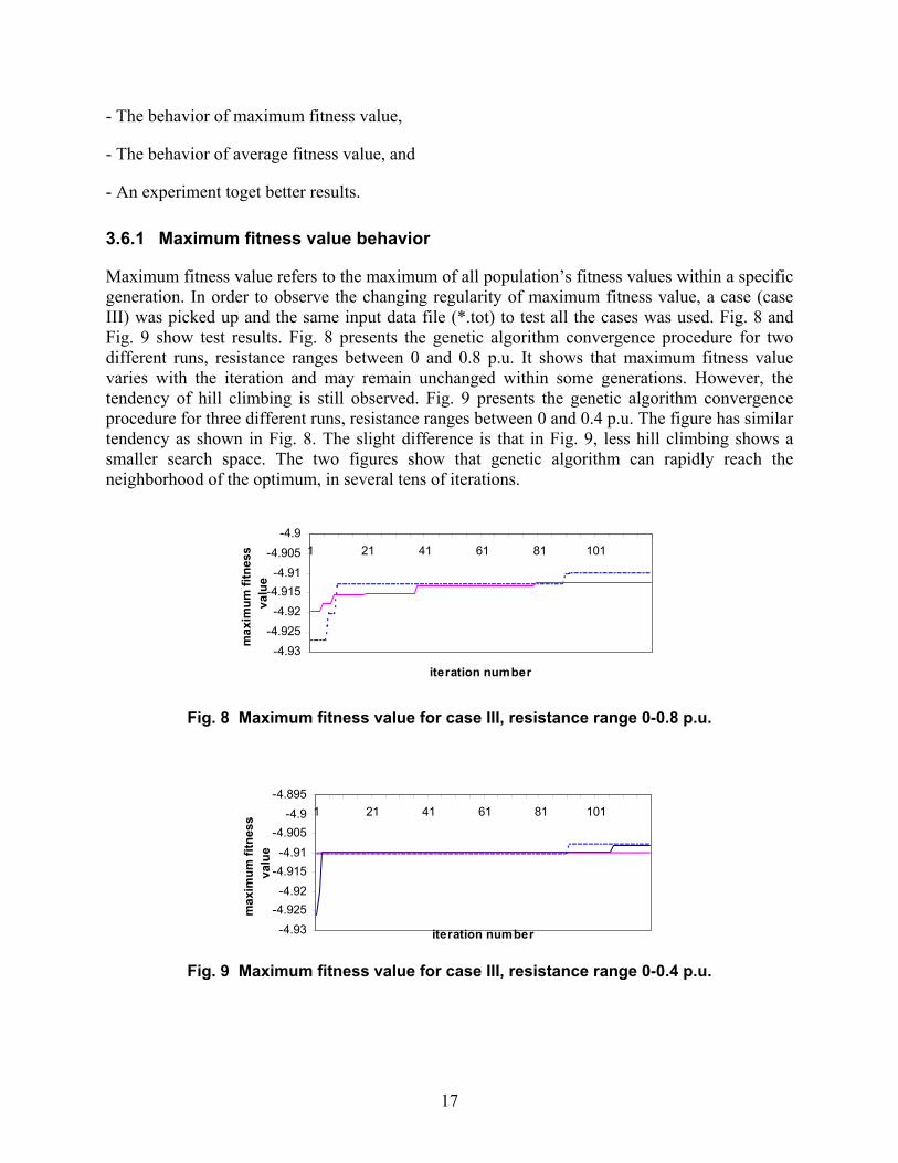
Maximum fitness value refers to the maximum of all population’s fitness values within a specific generation. In order to observe the changing regularity of maximum fitness value, a case (case III) was picked up and the same input data file (*.tot) to test all the cases was used. Fig. 8 and Fig. 9 show test results. Fig. 8 presents the genetic algorithm convergence procedure for two different runs, resistance ranges between 0 and 0.8 p.u. It shows that maximum fitness value varies with the iteration and may remain unchanged within some generations. However, the tendency of hill climbing is still observed. Fig. 9 presents the genetic algorithm convergence procedure for three different runs, resistance ranges between 0 and 0.4 p.u. The figure has similar tendency as shown in Fig. 8. The slight difference is that in Fig. 9, less hill climbing shows a smaller search space. The two figures show that genetic algorithm can rapidly reach the neighborhood of the optimum, in several tens of iterations.
-4.93-4.925-4.92
-4.915-4.91
-4.905-4.9
1 21 41 61 81 101
iteration number
max
imum
fitn
ess
valu
e
Fig. 8 Maximum fitness value for case III, resistance range 0-0.8 p.u.
Fig. 9 Maximum fitness value for case III, resistance range 0-0.4 p.u.
-4.93-4.925-4.92
-4.915-4.91
-4.905-4.9
-4.8951 21 41 61 81 101
iteration number
max
imum
fitn
ess
valu
e
18
It is difficult to determine if the estimated result is optimal. The only identification of the optimal solution is based on the fitness value. The smallest fitness value (in absolute value) within the search space corresponds to the optimum. However, for many cases we tested, the estimated results, obtained within a preset iteration number, locate the real fault location on a nearby section. Observing all test cases, some conclusions are listed as follows.
For every run, the convergence procedure may be different. The maximum fitness value may converge at a specific fitness value within a preset number of iterations. Although the approached fitness values for different runs may be almost the same, the corresponding estimated fault location might be assigned to entirely different sections. This situation may occur most frequently for short transmission lines. This phenomenon is consistent with the observation that the fitness surface can be very non-linear in specific cases. Increasing the number of iterations could be helpful in improving the accuracy of the estimated result and in decreasing the fitness value further. Increasing the region of fault resistance corresponds to enlarging the solution search space. Even if the ability of hill climbing is improved, the speed of convergence is still not increased. Average fitness value behavior
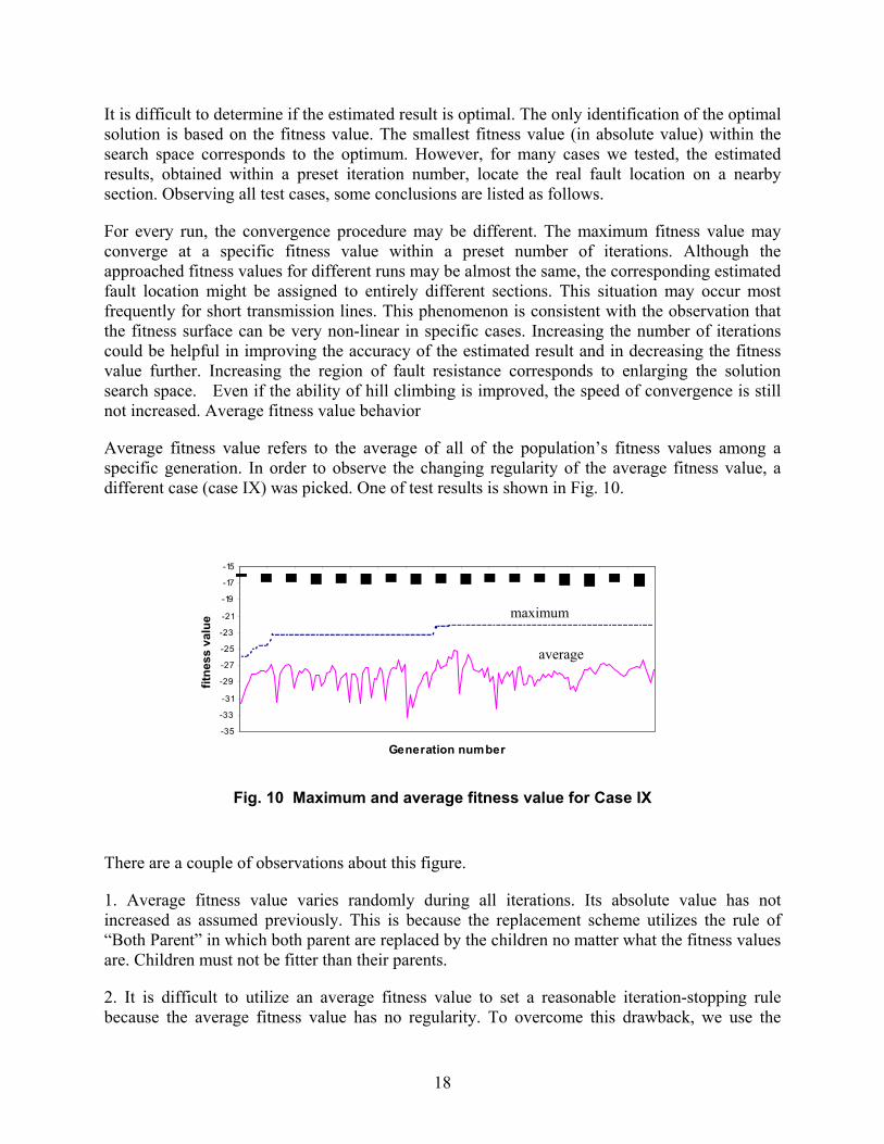
Average fitness value refers to the average of all of the population’s fitness values among a specific generation. In order to observe the changing regularity of the average fitness value, a different case (case IX) was picked. One of test results is shown in Fig. 10.
-35
-33
-31
-29
-27
-25
-23
-21
-19
-17
-15
Generation number
fitne
ss v
alue
Fig. 10 Maximum and average fitness value for Case IX
There are a couple of observations about this figure.
1. Average fitness value varies randomly during all iterations. Its absolute value has not increased as assumed previously. This is because the replacement scheme utilizes the rule of “Both Parent” in which both parent are replaced by the children no matter what the fitness values are. Children must not be fitter than their parents.
2. It is difficult to utilize an average fitness value to set a reasonable iteration-stopping rule because the average fitness value has no regularity. To overcome this drawback, we use the
maximum
average

19
replacement scheme of “Weak Parent” instead of “Both Parent”. In “Weak Parent”, the parent is replaced when the child is fitter than the parent.
The following test uses the scheme of “Weak Parent”. Fig. 11 shows the result of the same case (case IX). The average fitness value gradually approaches the maximum fitness value as the number of iterations increase. (The fitness value uses the absolute value in Fig. 11.) This characteristic can be utilized to add an additional termination criterion. When the relative error between the average fitness value and the maximum fitness value meets a specific threshold, iterating stops. The former criterion utilizes the fixed generation number as a preset threshold. A combination of these two criteria can form a new termination condition by forming a relationship of “OR” between the two criterions.
0
5
10
15
20
25
30
1 4 7 10 13 16 19 22 25 28 31 34 37
iteration number
fitne
ss v
alue
Fig. 11 Test results obtained from Case IX; two curves are obtained
by using the same input file (caseXI-1.tot)
After additional research on the new replacement scheme, we find that the above phenomenon always occurs except in one special case. In order to explain the exception, we have to be familiar with the GA iteration process. We set two parameters to control the production of initial population and the number of iterations ; they are “out_iteration” and “in_iteration”.
The latter parameter is used for the inner loop in which the initial population is produced randomly. The former parameter is used for the outer loop in which the initial population is produced randomly, except for keeping the best-obtained individuals. Usually the former parameter can be set to one (1). When the average fitness value equals or approaches the maximum fitness value, the result may be kept unchanged with the number of iterations changing. At this time, the parameter is useful in re-initializing the population.
When the parameter of “out_iteration” is set as a specific number (not equal to one), the changing of average fitness value is different from the result shown in the previous figure (Fig. 11). An example is shown in Fig. 12. In this case, we set out_iteration to 9 and in_iteration to 10; the total number of iterations is 90. The average fitness value decreases within an out_iteration, however there are some peaks among 90 iterations. In this situation, the termination using average fitness value cannot be used.
Average fitness
Maximum fitness

20
Fig. 12 Case IX (setting the “out_iteration” to 9, “in_iteration” to 10)
More tests show that the replacement scheme of “Weak Parent” can speed up convergence and help obtain more stable results. For example, for case III, using the new improved algorithm resulted in each run locating the same section. In general, result of every run cannot locate the same section if the previous replacement scheme of “Both Parents” is used for the same case.
3.6.2 Using a refined genetic algorithm
The crossover process randomly selects two parents to exchange genes with a crossover rate Pc. A higher crossover rate allows the exploration of the solution space around the parent solution.
The mutation process randomly selects one parent with a mutation rate Pm. The mutation rate controls the rate new genes are introduced, and explores new solution territory. If the mutation rate is low, the solution may settle at a local optimum. On the contrary, a high rate could generate too many possibilities. If the offspring lose their resemblance to the parents, the algorithm will not learn from the past and could become unstable.
In a refined genetic algorithm, the probabilities of crossover and mutation are variable for different generations. For every generation, probability of crossover is decreased linearly, while the probability of mutation is increased linearly. In order to contain these probabilities within a reasonable range, limits should be set so that they do not exceed permitted intervals.
In order to observe the performance of the refined GA, the case IX is tested thoroughly. The results are shown in Fig. 13 (The replacement scheme uses “Both Parent” in which children replace their parent whatever their fitness values are.) The first observation about the results shown in the figure is that the convergence is random and different for every run. For the same fitness value, (for example, -21.5) Fig. 13 shows only 20 iterations are needed for one run and 80 iterations are needed for another run. The second observation is that the change of maximum fitness values may remain static for a number of generations before a superior individual is found. The refined GA does not provide better performance. Theoretically, the refined genetic algorithm is superior to the normal genetic algorithm. For the same fitness value, the refined
0
5
10
15
20
25
30
1 7 13 19 25 31 37 43 49 55 61 67 73 79 85 91
iteration number
fitne
ss v
alue
Average fitness
Maximum fitness

21
algorithm can converge more quickly than the normal genetic algorithm. However, to the selection of the appropriate possibility of crossover and mutation should be done carefully.
Fig. 13 Fitness value for case IX, using refined GA, Pc (0)=0.9, Pm (0)=0.01
3.6.3 Conclusions regarding convergence
Because the GA is a stochastic search method, it is difficult to move away the randomness of the convergence process and specify the proper convergence criteria to make genetic algorithm search converge at the same solution for each run. Since the fitness of a population may remain static for a number of generations before a superior individual is found, the application of conventional termination criteria becomes problematic. A common practice is to terminate the GA after a pre-specified number of generations and then test the quality of the best members of the population against the problem definition. If no acceptable solutions are found, the GA may be restarted or a fresh search initiated.
Several convergence schemes can be utilized:
1. Fitness Sum - if the sum of the fineness over the population falls below the convergence criteria; 2. Average Fitness – when the population average falls below the criteria; 3. Best Gene – when the chromosome of best fit falls below the criteria; and 4. Worst Gene – when the worst chromosome falls below the criteria.
We have used the third scheme; the results show that the method is effective and helps obtain the more stable result. Of course, when a new replacement scheme (“Weak Parent” scheme in which the parent is replaced if the child is fitter than the parent) is adopted, the second one using average fitness value as the convergence rule is effective.
Theoretically, using the refined GA would help to approach optimal result quickly in most cases. We observe that some cases have the benefits. But it may not always be effective for all cases.
-27
-26
-25
-24
-23
-22
-21
-201 11 21 31 41 51 61 71 81 91 101 111
iteration number
fitne
ss v
alue

22
Moreover, increasing the number of iterations may help obtaining a better solution. However, we cannot increase the number of iterations without limit. Although the methods mentioned above may help improving the solution to some extent, a new more robust method needs to be introduced.
3.7 Conclusions
This section mainly describes the scheme of a general genetic algorithm with some improvements. The genetic algorithm convergence is discussed in detail and some corresponding test results are shown. A convergence criteria is suggested when the replacement scheme of “Weak Parent” is utilized.

23
4 IMPLEMENTATION OF THE FAULT LOCATION ALGORITHM
4.1 Introduction
This chapter gives an outline of the implementation of the fault location software. The architecture of the fault location software is presented first. Then the details of obtaining the accurately matched during-fault phasors and synchronizing the recorded phasors are given. Finally, the process of generating and tuning the static model is described.
During development of the fault location software, fifteen fault cases were tested. All test results and test analysis are presented in several interim reports submitted to PSERC. The following text refers to these reports.
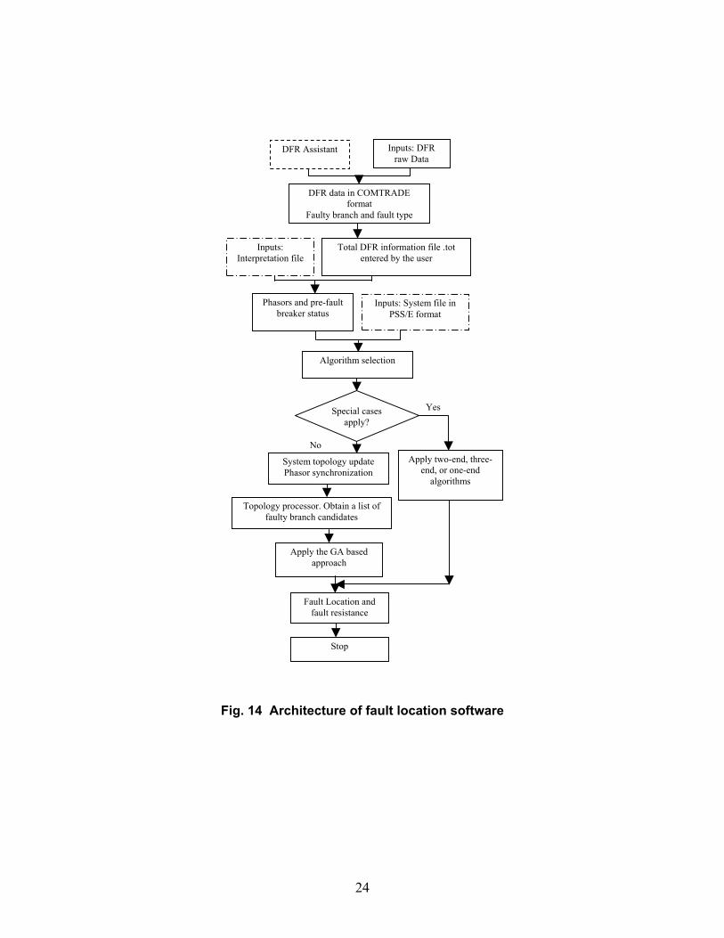
4.2 Architecture
The architecture of the fault location software is shown in Fig. 14. The input data include the DFR data, interpretation file, and the system model file in PSS/E format. The operation procedure of the software is briefly described, with a detailed illustration presented in succeeding sections.
In the case of CenterPoint Energy, specialized software called “DFR Assistant” converts the DFR raw data into COMTRADE format, and determines the fault type and faulted branches based on individual DFR recording [17]. Based on such information, the phasors of the monitored voltages and currents, pre-fault breaker status, and the total DFR information file can be obtained. Based on the interpretation file, a cross-reference between the designations used by DFR Assistant and the designations used by PSS/E can be found. The contents and generation of the DFR interpretation file and the total DFR information file will be illustrated later.
Based on the topology data and a number of available measurements, the fault location software determines the type of fault location algorithm to be utilized. In special cases when one-end, two-end, or three-end algorithms can be used, the fault location can be obtained directly based on the related voltage and current phasors without running PSS/E simulation studies. The approach for selecting the fault location algorithm is illustrated below.
Fig. 15 shows the system configuration used for one-end, two-end and three-end algorithms. The fault location software compares the actual system topology data and the available measurements with these configurations. If any of the configurations matches the actual case, then the matched one will be selected for fault location estimation. If none matches the actual case, then the genetic algorithm is selected for estimating the fault location.
24
Fig. 14 Architecture of fault location software
DFR data in COMTRADE format
Faulty branch and fault type
Total DFR information file .tot entered by the user
Phasors and pre-fault breaker status
Fault Location and fault resistance
DFR Assistant
Inputs: Interpretation file
Inputs: DFR raw Data
Inputs: System file in PSS/E format
System topology update Phasor synchronization
Algorithm selection
Special cases apply?
Apply two-end, three-end, or one-end
algorithms
Yes
No
Topology processor. Obtain a list of faulty branch candidates
Apply the GA based approach
Stop

25
Fig. 15 The selection of fault location algorithms
If the case belongs to the general case, then the following modules are to be executed.
• The current phasors and/or the pre-fault breaker status can be utilized to tune the system topology (update the static system model). Only the service status of the branch is updated. If the magnitude of the pre-fault current phasor of the monitored branch is smaller than a pre-specified value, then the branch is considered as being out of service. Branch status is also updated according to the pre-fault breaker status. If both the pre-fault breaker status and the current of a branch are monitored, the recorded current overrules the breaker status for determining the service status of the branch.
• After the system topology is updated, the PSS/E load flow study is carried out to obtain the pre-fault phasors of the related bus voltages and branch currents. Then, the phasors derived from the recorded waveforms are synchronized by a simple rotation with reference to the phasors obtained by the load flow study.
• Based on the faulty branches given by DFR Assistant and the system topology, the software derives the list of total faulted branch candidates for posing faults.
• The GA algorithm based approach is activated for searching the faults.
P
Fault
Q x
(b) One end algorithm
Fault
P Qx
(a) Two end algorithm
(c) Three end algorithm
Fault P Q
S
T
1L 2L
3L DFR

26
4.3 Obtaining phasors
Fourier transform is used for obtaining the pre-fault and during-fault phasors for the voltage and current measurements. Identification of the moment of fault inception is required before calculating the during-fault voltage and current phasors. The phasor of the voltage or current quantity during the fault is calculated from the waveform with reference to the pre-fault phasor. Fig. 16 illustrates the concept.
Fig. 16 Phasors obtained from the recorded waveforms The following nomenclature is used.
naR : the pre-fault phasor of phase a obtained from the recorded waveform
nbR : the pre-fault phasor of phase b obtained from the recorded waveform
ncR : the pre-fault phasor of phase c obtained from the recorded waveform
faR : the during-fault phasor of phase a obtained from the recorded waveform
fbR : the during-fault phasor of phase b obtained from the recorded waveform
fcR : the during-fault phasor of phase c obtained from the recorded waveform
Although the angle of the pre-fault phasor can be arbitrary because of the selection of the reference point when applying a Fourier transform, the difference between the angle of the pre-fault phasor and the angle of the fault phasor is fixed regardless of the reference point. In other words, if we rotate the real and imaginary axis as shown in Fig. 16, the angle between the phasor
naR and faR is unchanged. This is also true for phase b and phase c phasors. Using calculated pre-fault phasors could change topology of the static model locally. The pre-fault breaker status can be determined from the recorded digital channel status or the amplitude of calculated pre-fault phasors. The later is more reliable and it was used in the fault location software.
naR
faR
nbR
fbR
fcR
ncR
1+
j+

27
The calculation of the phasors based on the DFR recorded waveforms is illustrated using an example. Fig. 17 shows the three phase voltage waveforms.
Fig. 17 Three phase voltage waveforms
The following steps are taken to obtain the pre-fault and fault phasors of the voltage waveforms.
(1) One-cycle Fourier transform is applied to the entire voltage signal to obtain the rms voltage magnitude. The rms values of the signals are depicted in Fig. 18.
Fig. 18 RMS values of the voltage signals
0 0.05 0.1 0.15 0.2 0.25 0.3 0.35 -150
-100
-50
0
50
100
150
Time (Second)
Volta
ge (V
)
phase a phase b phase c
0 2 4 6 8 10 12 14 16 18 40
45
50
55
60
65
70
75
Cycl
rms
volta
ge (V
)
phase aphase bphase c

28
(2) Fault inception cycle is found by comparing the rms value cycle by cycle. (Fault
cycles are defined as the cycles after the fault inception. The fault inception cycles are determined from waveforms recorded by a DFR). In this case, the fault is found to start at the 13th cycle. For fault location purpose, the phasors at the 16th cycle will be utilized to ensure that the system has reached the steady state during the fault.
(3) The pre-fault phasors are calculated using the first cycle of the waveform. In this case the phasors are:
Phase a: 72.34 (-88.14 degrees) Phase b: 72.84 (152.48 degrees) Phase c: 73.28 (31.83 degrees)
(4) The phasors during the fault are calculated using the phase angle shift concept. The
magnitudes are calculated using the samples in the 16th cycle of the waveform. In this case, the magnitudes are:
Phase a: 40.74 V Phase b: 61.28 V Phase c: 54.43 V
The phase angle shift of the fault voltage signals is depicted in Fig. 19.
The phase angle shifts of the three phase voltages at the 16th cycle of the waveform are:
Phase a: 13.46 degrees Phase b: 13.42 degrees Phase c: -5.25 degrees
Therefore, the phasors during the fault are:
Phase a: 40.74 V (13.46 – 88.14 = -74.68 degrees) Phase b: 61.28 V (13.42 + 152. 48= 165.9 degrees) Phase c: 54.43 V (-5.25 + 31.83 =26.58 degrees)
The selection of the cycle for the calculation of the during-fault phasors may not always be optimal. Due to the lack of synchronization, it is difficult to select the cycle of the waveform that corresponds to the same period to calculate the during-fault phasors for different DFR recordings. This may bring about errors, especially for the arcing faults during which the fault resistance is changing. In other words, if the cycles of waveforms selected for calculating the during-fault phasors for different DFR recordings correspond to different fault conditions (such as different fault resistances), then there will be errors affecting fault location estimate.

29
Fig. 19 The phase angle shift of the voltage signals
4.4 Fault cycles
As mentioned above, fault location (FL) software determines fault cycles from the recorded waveforms. The purpose of finding the fault cycles is to obtain during-fault phasors which are then matched with during-fault phasors obtained through simulation. In certain cases, FL software may choose incorrect fault cycles. This may affect the calculation of phasors during the fault period. Obviously, the fault location results may be affected.
Note: The fault cycles are defined as the signal cycles after the fault inception. The fault inception moment is determined from the waveforms recorded by DFRs.
The detailed method is first to get currents from the DFR data file according to the preset order, and then calculate the amplitude of a specific phase (A phase) current cycle by cycle. The amplitudes of current calculated from different cycles will be compared with the reference value. If the amplitude of the current in a specific cycle increases over a preset threshold, the software considers the cycle to be the fault inception cycle or fault cycle. If the fault cycle for the specific signal phase cannot be found, other phases (B or C phase) are searched successively. If the fault cycle cannot be found on the specific circuit, the other circuits are searched successively until the fault cycle is identified. The method may fail under some situations.
For example, current waveforms for faulted circuit (Exxon Ckt.83) in case IV are shown in Fig. 20. This is a typical waveform of a single phase to ground fault in which B phase current increases during the fault, and waveforms of A and C phase almost do not change. If we use currents of the circuit to determine the fault cycle, using phase A does not result in finding the fault cycle. However, using B phase current can provide the correct result. The fault cycle is the 7th cycle from the start (trigger point) of the record.
0 2 4 6 8 10 12 14 16 18-6 -4 -2 0 2 4 6 8
10 12 14
Cycle
phase angle shift (degrees)
phase aphase bphase c

30
For the same fault, current waveforms on a specific circuit (other circuits, non-directly-faulted circuit) are significantly different, such as Dupont-Deer Pk Ckt.85 (Fig. 21). In this case (case IV), currents of phases B and C increase during the fault. The current of phase A decreases slightly during the fault, but increases after the fault is cleared. If we use the A phase current of the circuit to determine the fault cycle, an incorrect result is obtained. The fault cycle is the 14th cycle.
Because the fault occurs randomly, the fault cycle in a specific substation is determined according to a specific order, which is determined in the corresponding interpretation file. In the existing version of fault location software, the current used for calculating the fault cycle is chosen based on the sequence of analog channels in the interpretation files. Incorrect fault cycle may be obtained this way.
In an earlier version of the software, the fault inception cycle is determined through a series of tests on individual phase currents or voltages. For example, for a specific circuit, one first determines whether A phase current (or voltage) satisfies some test conditions. If the test conditions are not met, the software will continue with the B phase, then the C phase. If the fault inception cycle is not found on the first circuit, the next circuit will be analyzed using the same method until the fault inception cycle is found.
In some cases, the fault inception cycle calculation may be erroneous. The most common situation is when a single-phase-to-ground fault occurs; non-faulted-phase current may decrease during the fault and increase after the fault is cleared. If this phase happened to be analyzed first, the time instant of the current increase will be calculated as the fault instant (which is incorrect). This causes above-described method to fail. (This phenomenon has been explained above.)
The following cases are examples when the fault cycle was picked out incorrectly: cases I, IV, VI, XI.
Fig. 20 Case IV: current waveforms on Exxon Ckt.83 in Cedar Bayou
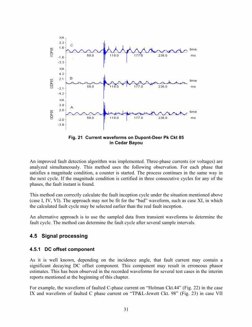
31
Fig. 21 Current waveforms on Dupont-Deer Pk Ckt 85
in Cedar Bayou
An improved fault detection algorithm was implemented. Three-phase currents (or voltages) are analyzed simultaneously. This method uses the following observation. For each phase that satisfies a magnitude condition, a counter is started. The process continues in the same way in the next cycle. If the magnitude condition is certified in three consecutive cycles for any of the phases, the fault instant is found.
This method can correctly calculate the fault inception cycle under the situation mentioned above (case I, IV, VI). The approach may not be fit for the “bad” waveform, such as case XI, in which the calculated fault cycle may be selected earlier than the real fault inception.
An alternative approach is to use the sampled data from transient waveforms to determine the fault cycle. The method can determine the fault cycle after several sample intervals.
4.5 Signal processing
4.5.1 DC offset component
As it is well known, depending on the incidence angle, that fault current may contain a significant decaying DC offset component. This component may result in erroneous phasor estimates. This has been observed in the recorded waveforms for several test cases in the interim reports mentioned at the beginning of this chapter.
For example, the waveform of faulted C-phase current on “Holman Ckt.44” (Fig. 22) in the case IX and waveform of faulted C phase current on “TP&L-Jewett Ckt. 98” (Fig. 23) in case VII
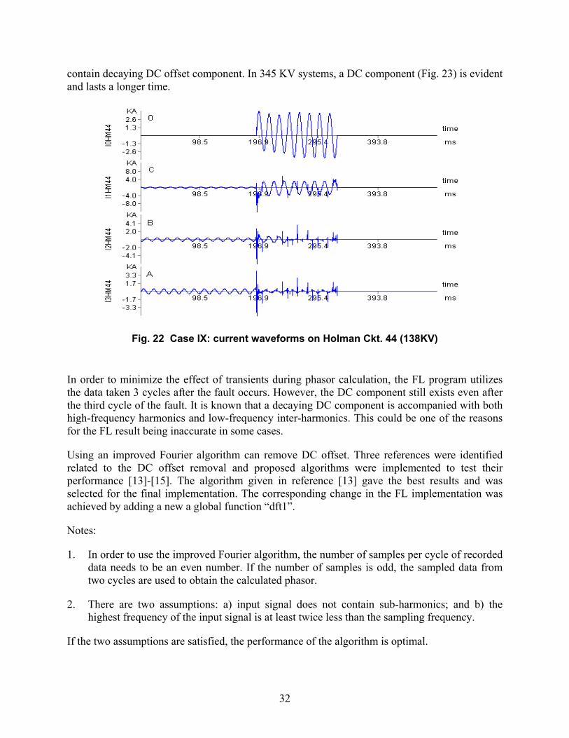
32
contain decaying DC offset component. In 345 KV systems, a DC component (Fig. 23) is evident and lasts a longer time.
Fig. 22 Case IX: current waveforms on Holman Ckt. 44 (138KV)
In order to minimize the effect of transients during phasor calculation, the FL program utilizes the data taken 3 cycles after the fault occurs. However, the DC component still exists even after the third cycle of the fault. It is known that a decaying DC component is accompanied with both high-frequency harmonics and low-frequency inter-harmonics. This could be one of the reasons for the FL result being inaccurate in some cases.
Using an improved Fourier algorithm can remove DC offset. Three references were identified related to the DC offset removal and proposed algorithms were implemented to test their performance [13]-[15]. The algorithm given in reference [13] gave the best results and was selected for the final implementation. The corresponding change in the FL implementation was achieved by adding a new a global function “dft1”.
Notes:
1. In order to use the improved Fourier algorithm, the number of samples per cycle of recorded data needs to be an even number. If the number of samples is odd, the sampled data from two cycles are used to obtain the calculated phasor.
2. There are two assumptions: a) input signal does not contain sub-harmonics; and b) the highest frequency of the input signal is at least twice less than the sampling frequency.
If the two assumptions are satisfied, the performance of the algorithm is optimal.

33
Fig. 23 Case XII: current waveforms on TP&L Jewett Ckt. 98 from
Limestone (345 KV)
4.5.2 High frequency noise
For some cases, the waveforms recorded by DFRs are severely polluted by high-frequency noise. This noise may result in a calculation error for the phasor estimation and consequently in a wrong fault location estimate.
For case I presented in the test report, the following waveforms were obtained from DFR files (Fig. 24). Obviously, the presence of the noise is such that the useful signals appear completely buried underneath.
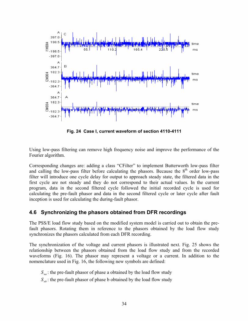
34
Fig. 24 Case I, current waveform of section 4110-4111
Using low-pass filtering can remove high frequency noise and improve the performance of the Fourier algorithm.
Corresponding changes are: adding a class “CFilter” to implement Butterworth low-pass filter and calling the low-pass filter before calculating the phasors. Because the 8th order low-pass filter will introduce one cycle delay for output to approach steady state, the filtered data in the first cycle are not steady and they do not correspond to their actual values. In the current program, data in the second filtered cycle followed the initial recorded cycle is used for calculating the pre-fault phasor and data in the second filtered cycle or later cycle after fault inception is used for calculating the during-fault phasor.
4.6 Synchronizing the phasors obtained from DFR recordings
The PSS/E load flow study based on the modified system model is carried out to obtain the pre-fault phasors. Rotating them in reference to the phasors obtained by the load flow study synchronizes the phasors calculated from each DFR recording.
The synchronization of the voltage and current phasors is illustrated next. Fig. 25 shows the relationship between the phasors obtained from the load flow study and from the recorded waveforms (Fig. 16). The phasor may represent a voltage or a current. In addition to the nomenclature used in Fig. 16, the following new symbols are defined:
naS : the pre-fault phasor of phase a obtained by the load flow study
nbS : the pre-fault phasor of phase b obtained by the load flow study

35
Fig. 25 The relationship between the phasors obtained by load flow study and by recorded waveforms
ncS : the pre-fault phasor of phase c obtained by the load flow study
α : the angle difference between the phasor obtained by the load flow study and the phasor obtained from the recorded waveform.
Synchronization is done by rotating counterclockwise the fault phasors faR , fbR and fcR by an angle of α . All DFR data are synchronized to the simulated phasors in the same way. As a result, all the DFR data can be synchronized.
In the above programs, the commands “FNSL, OPT” are used to perform the load flow studies using the Newton-Raphson method. The pre-fault voltage and current quantities are obtained using commands such as BUSDAT, BRNCUR, BRNFLO and BRNMVA. BUSDAT is used to obtain the bus voltages. BRNCUR, BRNFLO and BRNMVA are used to obtain the branch currents. The voltage and current quantities are saved in a file with pre-specified name that will be interpreted and processed by the C++ programs.
4.7 Processing the static model
The given static system model, used in simulation studies, may not reflect the prevailing operating conditions of the system when the fault occurs. To match the phasors extracted from DFRs and those obtained from simulation studies, it may be beneficial that the system model used in studies be updated by utilizing the information captured close to the moment when the fault occurs. The process of updating the system model is called “the tuning of the system model.”
naS naR
faR
nbS
nbRfbR
fcR
ncR
ncS
α
1+
j+

36
Tuning of the system model may include updating the topology as well as the generation and load data of the system. The pre-fault data, including the pre-fault phasors and breaker status, provided by DFRs may be used for the tuning process.
4.7.1 Determining the topology
4.7.1.1 Read topology data
The CenterPoint Energy transmission system is described in PSS/E file format. The topology (i.e., connectivity between different buses), line status (whether the line is in service or not), line impedances, and susceptances are extracted from the original file. A module called “topology processor” realizes such functionality. A sample system shown in Fig. 26 is used to illustrate the processing of the topology data.
Based on this diagram, the following information is obtained and saved in appropriate files.
• Connectivity is described as shown in the following table: 100 8 8 100 3 -99 (a minus sign indicates a transformer) 3 5 5 8 5 3 3 43 2 2 5 6 7 99 99 7 -8 43 43 99 5 -10 10 -43 6 2
For example, the line “8 100 3 -99 (a minus sign indicates a transfomer)” denotes that bus 8 is connected with bus 100 and bus 3 through a line, and connected to bus 99 through a transformer.
Fig. 26 A sample system
100 8 3 5 2 6
7 99 43
10
1
2 transformer
bus
line

37
• Branch service status is described as shown in the following table (only not-in service branches are included):
3 5 2
This means that the branch 2 between the bus 3 and 5 is out of service.
• Branch Impedances and Susceptances (including both the zero sequence and positive sequence quantities) are obtained as shown in the following table:
100 8 0.01 0.02 0.015 0.1 0.2 0.01 8 3 0.1 0.1 0.03 0.2 0.25 0.02 …
For example, the first line reads “the line between bus 100 and bus 8 has positive sequence impedance of 0.01+j0.02 p.u., positive sequence susceptance of 0.015 p.u., zero sequence impedance of 0.1+j0.2 p.u., and zero sequence susceptance of 0.01 p.u.
4.7.1.2 Topology Modification
Based on the pre-fault breaker status and the pre-fault current magnitudes of the monitored branches derived from the DFR data, the service status (i.e., in or out of service status in the static model saved in the PSS/E file) of the branches will be updated. A zero magnitude (or smaller than 0.01 p.u.) of the current through a monitored branch indicates an out-of service status of the branch. If both the current and the breaker status of a branch are available, the current measurement will be used instead of the breaker status for topology update. This is based on the observation that the monitoring of currents is usually more reliable than the monitoring of the breaker status because the measured contacts of the breaker themselves may misoperate or may not be monitored.
The topology modification is realized using the IPLAN language, which is part of the PSS/E package [18]. The IPLAN language is able to modify the system topology, control the load flow and short circuit studies, and control the reporting of the results of the PSS/E activities. Like other programming languages, IPLAN language can be used to write programs by which one can automatically control the PSS/E activities, read and save the results in a disk file. The IPLAN language facilitates the interaction between the PSS/E activities and C++ programs.
The following program illustrates how the IPLAN language is used to modify the system topology.
PROCEDURE updateSY QPUSH 'MENU,OFF' QPUSH 'CASE' QPUSH OldSave QPUSH 'chng' QPUSH '3' LOOP i = 1 TO in_ser QPUSH in_bus1_i(i),',',in_bus2_i(i),',',in_ckt(i) QPUSH '1' QPUSH '1' QPUSH '0' QPUSH '0' ENDLOOP

38
LOOP i = 1 TO out_ser QPUSH out_bus1_i(i),',',out_bus2_i(i),',',out_ckt(i) QPUSH '1' QPUSH '0' QPUSH '0' QPUSH '0' ENDLOOP QPUSH '-1' QPUSH 'SAVE' QPUSH NewSave RETURN END
In this program, “OldSave” is the original file containing the system model. The IPLAN command “chng” is used to update the service status of all the branches whose actual status differs from the status indicated in the original model. The actual status refers to the status obtained from the DFR recordings based on the pre-fault breaker status and the current magnitudes of the monitored branches. The updated model is saved in a new file named “NewSave”. The branches whose status needs to be modified are determined by C++ program and passed to the IPLAN program. The IPLAN program can be invoked inside the C++ program. This is accomplished by using the following C++ program scripts.
void callexe(char *prog, char *args) _ spawnl(_P_WAIT, prog, prog, args, NULL); Void invoke_Psse () callexe("x:\\pti\\psse26\\pssexe\\psslf4", "-gnikool off -buses 4000 –inpdev g:\\users2\\liaoy\\ly\\psse\\flocini.idv"); //File: flocini.idv EXEC c:\windows\profiles\liaoy\desktop\update @END
The interaction between the C++ program and the PSS/E application software can be achieved using the described approach.
4.7.2 Tuning static system
4.7.2.1 When additional data are not available
In this situation, only limited DFR data can be used to tune the generator and load data.
(1) Approach I
The objective function should be determined first. The goal of updating the generator output power and load power is to make the static system model closer to the real life system at the time before the fault occurs. To reach the goal, the waveform-matching based approach is utilized. The matching is made between the voltage and current waveforms obtained by DFR and those generated in power flow studies.

39
To evaluate the matching degree of the simulated and recorded waveforms, the following criteria is utilized,
∑∑==
−+−=iN
kkrkski
Nv
kkrkskvc IIrVVrf
11
&&&& (4.1)
where
cf : the objective function or the defined cost function
kvr and kir : the weights for the errors of the voltages and currents respectively
ksV and krV : the pre-fault voltage phasors obtained from the load flow calculation and recorded waveforms respectively
ksI and krI : the pre-fault current phasors obtained from the load flow calculation and recorded waveforms respectively
vN and iN : the total number of the voltage and current phasors respectively
The meaning of ksV , krV , ksI and krI in equation above is different from the one in equation (2.2).
The final goal of updating generator output power and load power is to minimize the function shown in equation (4.1).
Second, all generator nodes and load nodes related to the triggered DFRs are searched. The details are illustrated as described below.
The generator nodes can be searched among the substations where DFRs were triggered. All buses in the substation where the DFRs were triggered should be easy to find. These buses may be the extended buses of remote buses whose voltage is controlled by corresponding generators. The generator nodes can be obtained through matching these buses with the extended buses in the power flow raw data file and picking the corresponding generator node buses.
Then, load buses should be searched through introducing the “search depth” concept. The “search depth” is defined as the number of lines on a certain search path starting from a specified bus. The search depth is used as a constraint in the search process. Here, starting search buses are those buses that are included in the substation with triggered DFRs. After obtaining a list of total possible load buses, real load buses should be picked through comparing the load buses in the power flow raw data file.
Third, the tuning strategy should be determined.
The simplest probing method is to tune the generator and load data according to a specific rule. The following rule is applied in determining the individual load and generator power: “Adjust

40
the power such that, at each load or machine, the ratio of individual load or machine power to the total power of all buses, loads or machines being processed remains unchanged.”
After the generator power and load power are tuned, then determine whether the tuning is effective. If the tuning is effective, we can continue the tuning according to the direction of the increase until the best match between the pre-fault load and simulated power flow is achieved. Otherwise, perform updating of the generator output power and load power pursuing the opposite direction. The flowchart of tuning the static system model is shown in the Fig.27.
Obtaining the bus number of substations whereDFR were triggered
Obtaining the generator bus number of thesubstation based on the above information
Using a specified “search depth” obtain a list ofthe load bus numbers
Obtaining the generator data
Increasing the output power of generatorsand the load power based on a specific rule
Decreasing the output power of generatorsand the load power based on a specific rule
Calculating load flow using PSS/E
Calculating the fitness value
Fitness value is decreased?
Reaching preset model numbers?
End
Calculating load flow using PSS/E
Calculating the fitness value
Fitness value is decreased?
Reaching preset model numbers?
End
Y
Y
Y
Y
N
NN
N
Fig. 27 The flowchart of tuning static system model

41
Table 1 shows the change of fitness value before and after tuning for the case IV. The table includes a total of six cases using different DFR files and the different matched quantities.
In Table 1, the first column represents the different combinations of DFRs. The second column shows the fitness value calculated using the pre-fault phasor. The first value in the second column is obtained using the untuned system model. The second one is obtained using tuned system model, which is produced based on the adjusting strategy mentioned above. Using the same tuned system model, the fitness values are obtained by matching during-fault phasor and they are listed in the third column. In order to observe the effect of model tuning and compare to the fitness value obtained by using the static model, the fitness values calculated using the pre-fault phasor and static model are also listed in the third column.
When the fitness value is close to zero, the recorded waveform fits the simulated waveform completely. We can then say that the tuning strategy is effective once the fitness value has the tendency to approach zero. In Table 1, the third column shows that the fitness value has a tendency to decline. This may explain why the tuned model is closer to the actual operation condition than the static model. The extent of decrease depends on the region of tuning.
Table 1 – The change of fitness value before and after tuning for Case IV
DFR Files Utilized
Fitness value using pre-fault phasor before and after model
tuning
Fitness value using during-fault phasor before and after
model tuning
Quantities matched
Event 870 15.499→9.289 39.48→34.57 All monitored currents
Event 870 5.344→0.527 10.24→7.72 Currents on affected Ckt. 74
Event 870 Event 877 35.492→26.431 60.32→58.49 All currents
Event 870 Event 877 7.361→0.906 13.96→11.25 Currents on affected
Ckt. 74 and Ckt. 98
Event 870 15.707→9.497 41.72→38.41 All currents and all voltages
Event 870 Event 877 35.806→26.745 62.01→60.18 All currents and all
voltages
(2) Approach II
The objective function remains the same as shown in equation (4.1). The criterion is used to evaluate the degree of matching between the recorded pre-fault waveform and simulated pre-fault waveform obtained from the updated system model. The best match corresponds to the model that could reflect the real system operating condition just before the fault occurs.
It is easy to conclude that the problem is actually a problem of finding an optimum. The goal is to obtain an optimal model instead of the original system model. This is hard to achieve since the parameters of the generators and loads, the number of loads and generators, and the system topology may be changing all the time. Therefore, it is more desirable to obtain a better model as opposed to looking for a model that permits the optimal matching according to the criterion.

42
In the former strategy, a new problem is that the tuned system model may not always keep the load flow convergence. Based on the former tuning strategy, generator and load data are updated according to a specific rule. After the system parameters are updated, the software must check the fitness value obtained by matching the pre-fault phasors.
In Fig. 27, once the calculated fitness value is no longer decreasing, the tuning operation stops. When the tuning scope or tuning ratio becomes large, the corresponding load flow for the tuned system model may not converge. Therefore, a step to check the load flow convergence is added into the program.
With the running of the fault location software, an additional problem occurs. The problem is that the load flow convergence is not related to the tuning ratio. It is possible that, for a specific ratio, the load flow will converge. Continuing updating the ratio according to the tuning trend, the load flow may diverge. After that, the load flow may become convergent again.
In the former version of the tuning system, only the generators located at the substations where the DFRs have triggered are tuned. It is known that usually several DFRs could be triggered by a specific fault. Sometimes, only one DFR is triggered. Under this condition, the number of tuned parameters is too small to make a meaningful change. The details are as follows.
First, the tuned generator buses and load buses should be picked up.
To obtain the generator buses, the station buses of the monitored substations should be obtained by searching the corresponding interpretation files. These buses are the generators’ extended buses (behind the step-up transformer). The generator’s bus number will be obtained through searching the load flow raw data file.
To obtain the load buses, the concept of a search layer mentioned earlier is applied. In the substations where DFRs have triggered, station buses can be obtained through reading the interpretation files. The branches connected to these buses are the first layer. The other layer can be derived from these branches. The tuned load bus number finally is obtained through checking the branch’s ‘from’ and ‘to’ bus.
The tuned parameters of generators and loads are obtained through searching the load flow raw data file thoroughly.
The tuning strategy is to first preset a step for active and reactive power, such as 1% of rated active and reactive power. Then, specific updated models are generated through modifying the power of generators and loads. For the load, the ratio of active and reactive power remains fixed in order to make the load flow converging easily.
The change for each generator or load is different. After the parameters of the generators are updated, it has to be determined whether they are in the range of the power output. If the power is more than the upper limit, the power output is set as a maximum power output. If the power is lower than the lower limit, the power output is set as a minimum power output. For the loads, the power has no fixed limit; the minimum is set as zero. The ratio of reactive over active power remains the factor under the rated condition.

43
In our case, a total of 60 updated models are generated. Then, the PSS/E is invoked to calculate the load flow. The total mismatch in the whole set of updated system models is used to determine whether the load flow converges. Those updated models in which the load flow is not convergent for are ignored.
Calculating the fitness value using the pre-fault phase for matching compares the rest of the models plus the original static system model. The minimum fitness value is found and the corresponding model is the one we find. The flow chart is shown in Fig. 28.
Obtaining the bus number of all monitored substations
Obtaining the generator bus number in the substation basedon the above information
Using a specified “search depth” to obtain a list of the loadbus number
Obtaining the generator parameters by invoking the IPLANprogram “gen_loadbus.irf”
Tuning the selected generator and load data based on aspecific strategy
Calculating load flow using an updated system model
Convergent?
Calculating the fitness value
Generating enough models?
Picking a maximum fitness value and obtaining correspondingindex of updated model
Obtaining a list of parameters for the selected system model
Saving the selected model
End
N
N
Fig. 28 The flowchart for local tuning of the static system model

44
As a final note, the key to these two approaches is to keep the balance between the tuned generator and load data. This point is a necessary condition to make the power flow convergent.
4.7.2.2 When additional data are available
Comparing with the approach presented in section 4.7.2.1, the alternative approach is to use additional real time data to tune the static system model. In PSS/E model, a static system model usually can be divided into many areas. For each area, the generator data in an hour or half an hour before the fault occurs may be provided. These real time data can be helpful in improving the static system model accuracy.
Because additional real data have not been obtained for this project, the following statement is only for giving an outline of a possible future approach.
The software routine (in PSS/E) “SCAL” can be utilized to modify the total load, generation (positive generator power), motor load (negative generator power), bus connected capacitors, and/or bus connected reactors in a specified subsystem of the working case. The entire working case is scaled when the suffix ALL is specified when invoking SCAL. Otherwise, the user selects the subsystem to be processed based upon the suffix specified. If only a specific area is scaled, the suffix AREA is specified.
Here is the detailed procedure to follow. Before running the fault location software to estimate a fault location, the additional generator power in the whole network or some specific areas should be changed according to the information provided by utilities. These data are real time measurements in an hour or half an hour before the fault occurs. Then, activity “SCAL” is executed in PSS/E. The total change of load data should be equal to the total change of the generator data. The changed system model will replace the static system model and PSS/E will use the changed one to simulate faults.
4.8 Conclusions Two main factors may affect the accuracy of the fault location estimate. One is the correct calculation of the fault cycle combined with synchronization of recorded phasors. Another is the model utilized for carrying short circuit study, which should reflect the real system operation condition when a fault occurs. The efforts of obtaining more accurate recorded phasors and static model can lead to more accurate fault location estimates.
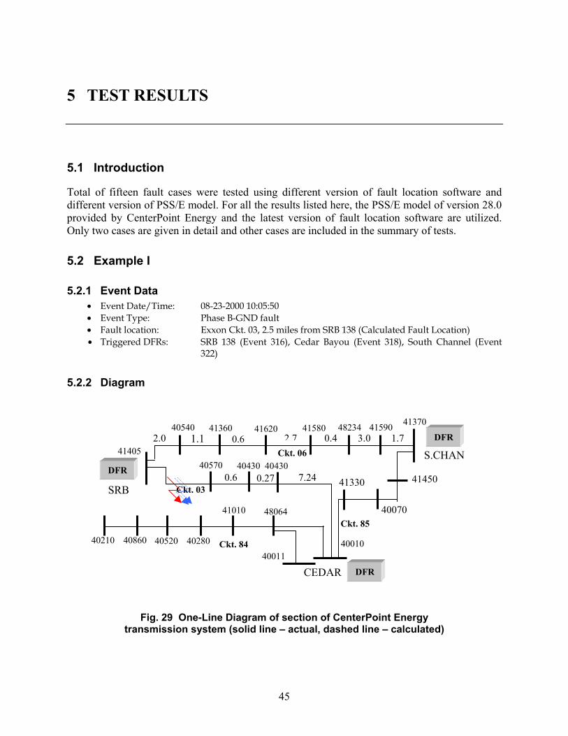
45
5 TEST RESULTS
5.1 Introduction
Total of fifteen fault cases were tested using different version of fault location software and different version of PSS/E model. For all the results listed here, the PSS/E model of version 28.0 provided by CenterPoint Energy and the latest version of fault location software are utilized. Only two cases are given in detail and other cases are included in the summary of tests.
5.2 Example I
5.2.1 Event Data • Event Date/Time: 08-23-2000 10:05:50 • Event Type: Phase B-GND fault • Fault location: Exxon Ckt. 03, 2.5 miles from SRB 138 (Calculated Fault Location) • Triggered DFRs: SRB 138 (Event 316), Cedar Bayou (Event 318), South Channel (Event
322)
5.2.2 Diagram
Fig. 29 One-Line Diagram of section of CenterPoint Energy transmission system (solid line – actual, dashed line – calculated)
40011
SRB
CEDAR
S.CHAN 41405
41370
40010
40570 40430
40540 41360 41620 41580 48234 41590 DFR
DFR
DFR
Ckt. 03
Ckt. 06 2.0 1.1 2.70.6 0.4 3.0 1.7
Ckt. 85
0.6 7.24 41450
40070
41330
404300.27
48064 41010
40280 40520 40860 40210 Ckt. 84
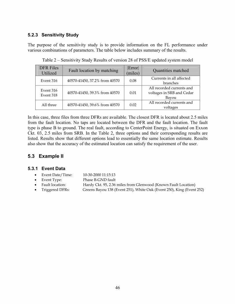
46
5.2.3 Sensitivity Study
The purpose of the sensitivity study is to provide information on the FL performance under various combinations of parameters. The table below includes summary of the results.
Table 2 – Sensitivity Study Results of version 28 of PSS/E updated system model
DFR Files Utilized Fault location by matching |Error|
(miles) Quantities matched
Event 316 40570-41450, 37.2% from 40570 0.08 Currents in all affected branches
Event 316 Event 318 40570-41450, 39.3% from 40570 0.01
All recorded currents and voltages in SRB and Cedar
Bayou
All three 40570-41450, 39.6% from 40570 0.02 All recorded currents and voltages
In this case, three files from three DFRs are available. The closest DFR is located about 2.5 miles from the fault location. No taps are located between the DFR and the fault location. The fault type is phase B to ground. The real fault, according to CenterPoint Energy, is situated on Exxon Ckt. 03, 2.5 miles from SRB. In the Table 2, three options and their corresponding results are listed. Results show that different options lead to essentially the same location estimate. Results also show that the accuracy of the estimated location can satisfy the requirement of the user.
5.3 Example II
5.3.1 Event Data • Event Date/Time: 10-30-2000 11:15:13 • Event Type: Phase B-GND fault • Fault location: Hardy Ckt. 95, 2.36 miles from Glenwood (Known Fault Location) • Triggered DFRs: Greens Bayou 138 (Event 251), White Oak (Event 250), King (Event 252)

47
5.3.2 Diagram
Fig. 30 One-Line Diagram of section of CenterPoint Energy
transmission system (solid line – actual, dashed line – calculated)
5.3.3 Sensitivity study
The purpose of the sensitivity study is to provide information on the FL performance under various combinations of parameters. The table below includes summary of the results.
Table 3 – Sensitivity Study Results
DFR Files Utilized
Fault location by matching
|Error| (miles) Quantities matched
Event 251 Event 250 Event 252
40620-48295 and 31.6% from 40620 0.48 All currents
Event 251 Event 250 Event 252
40620-48295 and 35.5% from 40620 0.24 All currents and all voltages
Event 251 Event 252
40620-48295 and 37.2% from 40620 0.15 All currents
In this case, three files from three DFRs located at different substations are available. The closest DFR (located at Green Bayou) is situated at 4.54 miles from the fault location. One tap is located between the DFR and fault location. According to data received from CenterPoint Energy, actual location is at 2.36 miles from Glenwood. Results listed in table 3 show that the three estimated locations using different options (different DFR combination and different matched quantities) are close to the actual one, their accuracy is deemed reasonable.
Greens Bayou 138
DFR 3.4 4.3 2.1
40900
40180 466104584048295 45850
Ckt. 97
7.5
3.0
10.1
40710
6.0 0.9
40620 Gl
DFR
White Oak
DFR 40255
40710
45630

48
5.4 Summary of results
Test results for all fifteen fault cases are listed in Table 4.
Table 4 – Test results for 15 fault cases
Case # Numb er of DFR triggered
Actual or calculated fault location
Estimated fault location Error
1 2 41111-41700 0.40 mile
41111-41700 0.2 mile 0.2
2 2 48402-40590 3.32 miles
48402-40590 3.63 miles 0.3
3 1 41300-48386 3.49 miles
41300-48386 3.15 miles 0.3
4 3 40570-41405 2.50 miles
40570-41405 2.47 miles 0.0
5 1 46262-48306 2.0 miles
46262-48306 1.18 miles 0.8
6 1 46570-48219 1 mile
46570-48219 0.1 mile 0.9
7 1 46570-48219 2.8 miles
46512-4830 6.1 miles 3.3
8 1 46262-48306 3 miles
46262-48306 5.7 miles 2.7
9 1 5915-9073 66.0 miles
5915-9073 66.9 miles 1.0
10 1 45840-40180 3.8 miles
40180-40620 0.4 mile 0.9
11 3 40620-48295 2.36 miles
40620-48295 2.13 miles 0.2
12 2 46020-3390 7.77 miles
46020-3390 6.54 miles 1.2
13 2 46020-3391 7.77 miles
46020-3391 6.2 miles 1.6
14 2 46020-3391 7.77 miles
46020-3391 4.77 miles 3.0
15 2 46020-3390 7.77 miles
46020-3390 7.09 miles 0.7
5.5 Conclusions
Fifteen fault cases are tested thoroughly and corresponding results are listed in Table 4. In this table, all triggered DFR files are involved and all monitored currents and voltages are utilized for matching. Most of the test results judged to be reasonably accurate.

49
6 CONCLUSIONS
This document mainly presents the algorithm, module and test results of the suggested fault location algorithm. All results are related to fifteen test cases provided by CenterPoint Energy. Although the test results listed in this document are for just a few cases and cannot be assume to express software performance completely, test results are quite good. Some conclusion and suggestion are given below.
Test results show that that accuracy of the fault location estimate is related to several factors. The number of DFRs triggered is one. Having more DFRs triggered is helpful in improving the accuracy. Under the situation when multiple DFRs are triggered, determination of the fault inception cycle is another key to the accuracy. For a specific case, if a different DFR is used with a different fault inception cycle to calculate the during-fault recorded phasors, additional error will be introduced.
Test results show that a specific case is sensitive to the fault search region, especially in 345KV system. Based on test results, the fault resistance range is recommended to set be 0-0.4 p.u. (actual value 0-76 Ω) or less in 138KV, 0-0.05 p.u. (actual value 0-60Ω) or less in 345KV systems.
Test results show that using all monitored currents and voltages for matching is a good choice. Using only a few selected quantities for matching may lead to an error in determining the fault location.
Test results show that updated model can help improve the accuracy of the fault location estimate for most cases. More benefits will be obtained if real power flow is obtained at the time fault occurs.
The actual faulted branch (section) must be included in the list of candidates. Otherwise, estimated fault location never reaches the actual fault location.
50
7 REFERENCES
[1] A.A. Girgis and M.B. Johns, “A hybrid expert system for fault section identification, fault type
classification and selection of fault location algorithms”, IEEE Transactions on Power Apparatus and Systems, vol.4 , no.2, April 1989.
[2] M.Kezunovic, I.Rikalo, C.W.Fromen, D.R.Sevick, S.M.McKenna,”Automatic fault analysis using intelligent techniques and synchronized sampling”, in Proceeding of the CIGRE General Session, Paris, France, September 1998.
[3] M.S. Eriksson, and G.D. Rockfeller, “An accurate fault locator with compensation for apparent reactance in the fault resistance resulting from remote-end infeed”, IEEE Transactions on Power Apparatus and Systems, PAS-104, no.2, Feb. 1985.
[4] Q. Zhang, Y. Zhang, W. Song, and D. Fang, “Transmission line fault location for single-phase-to-earth fault on non-direct-ground neutral system”, IEEE Transactions on Power Delivery, Vol. 13, no.4, Oct. 1998.
[5] D. Novosel, D. G. Hart, E. Ud, and J. Garitty, “Unsynchronized two-terminal fault location estimation”, IEEE Transactions on Power Delivery, vol. 7, no.1, January 1992.
[6] A.A. Girgis, D. G. Hart and W.L. Peterson, “A new fault location technique for two-and three-terminal lines”, IEEE Transactions on Power Delivery, vol. 7, no. 1, January 1992.
[7] D. L. Waikar, S. Elangovan, and A.C. Liew, “Fault impedance estimation algorithm for digital distance relaying”, IEEE Transactions on Power Delivery, vol. 9, no.3, July 1994.
[8] Y. Liao and S. Elangovan, “Digital distance relaying algorithm for first-zone protection for parallel transmission lines”, IEE Proceedings-Part C: Generation, Transmission and Distribution, vol. 145, no. 5, Sept 1998
[9] M. Kezunovic and B. Perunicic, “Automated transmission line fault analysis using synchronized sampling at two ends”, IEEE Transactions on Power Systems, vol. 11, no.1, pp. 441-447.
[10] Z. Q. Bo, A. T. Johns, and R. K. Aggarwal, “A novel fault locator based on the detection of fault generated high frequency transients”, Sixth International Conference on Developments in Power System Protection, Nottingham, England, March 1997.
[11] Z.Q. Bo, G.Weller, M.A. Redfern, “Accurate fault location technique for distribution system using fault-generated high-frequency transient voltages signals”, IEE Proc. Gener. Transm. Distrib. Vol. 146, No. 1, January 1999.
[12] Power technologies, Inc. “PSS/E-27 program operation manual “, December, 2000 [13] M. Kezunovic, Yong Guo, “Simplified Algorithms for Removal of the Effected of Exponentially
Decaying DC-offset on the Fourier Algorithm,” (to be published) in IEEE Transactions on Power Delivery.
[14] Jun-Zhe Yang, Chiu-Wen Liu, “Complete Elimination of DC Offset in Current Signals for Relaying Applications”, Power Engineering Society Winter Meeting, 2000 IEEE, Volume 3, PP1933-PP1938.
[15] Jhy-Cherng Gu, Sun-Li “Removal of DC Offset in Current and Voltage Signals Using a Novel Fourier Filter Algorithm”, IEEE Trans. On Power Delivery, Vol.1, No.1, January 2000.
[16] David E. Goldberg, “Genetic algorithms in search, optimization and machine learning”, Addison-wesley Publishing Company, INC, 1989.
[17] Test Laboratories International, Inc. “DFR assistant- software for automated analysis and archival of DFR records with integrated fault location calculation”, [Online] http://www.tli-inc.com
[18] Power technologies, Inc. “IPLAN program manual “, December, 2000.


![Accurate Fault Modeling and Fault Simulation of Resistive ...faculty.cs.tamu.edu/walker/pubs/sardessai98.pdf · The bridging fault simulator proposed by [8] is based on accurate modeling](https://img.pdfslide.net/doc/110x75/5f57d134e454a8594468c8f4/accurate-fault-modeling-and-fault-simulation-of-resistive-the-bridging-fault.jpg)