Advanced Analysis Methods for3G Cellular Networks

Jaana Laiho, Kimmo Raivio, Pasi Lehtimaki, Kimmo Hatonen, Olli Simula

Abstract— The operation and maintenance of the 3G mo-bile networks will be challenging. These networks will bestrongly service driven, and this approach differs signifi-cantly from the traditional speech dominated 2G approach.Compared to 2G, in 3G the mobile cells interact and inter-fere with each other more, they have hundreds of adjustableparameters, and they monitor and record data related toseveral hundreds of different variables in each cell.

This paper shows that a neural network algorithm calledthe Self-Organizing Map (SOM) together with a conven-tional clustering method like the k-means can effectively beused to simplify and focus network analysis. It is shown thatthese algorithms help in visualizing and grouping similarlybehaving cells. Thus, it is easier for a human expert to dis-cern different states of the network. This makes it possibleto perform faster and more efficient trouble shooting andoptimization of the parameters of the cells. The presentedmethods are applicable for different radio access networktechnologies.

Keywords— Network management, 3G cellular system,WCDMA, radio access network, artificial neural network,Self-Organizing Map, k-means clustering, data mining.

I. Introduction

The mobile communication industry is currently shiftingits focus from second generation networks (2G) towardsthe third generation networks (3G). The shift is not onlyrelated to the evolution of the access technology, but alsoto the vision of the development of service provisioningand service demands, customer expectations and customerdifferentiation.

While current wireless networks still evolve and ser-vice providers bring new internet packet data servicesinto the markets, an increasing number of operators andother wireless communication professionals are becomingfamiliar with the wideband code division multiple access(WCDMA) technology and prepare themselves for 3G ser-vices and networks. There will be a number of new chal-lenges when shifting from the current 2G to the new 3Gnetworks, many of them related to the design and the op-eration of true multi-service radio networks. An essentialpart of the new challenges is related to the provisioning,monitoring and optimization of the services. The numberof network counters and measurements shall increase owingto the fact that instead of monitoring GSM voice only, onemust concentrate on monitoring multi system and multi-service environment. The information space of future net-

J. Laiho and K. Hatonen are with Nokia Group, FinlandK. Raivio, P. Lehtimaki and O. Simula are with the Neural Net-

works Research Centre, Helsinki University of Technology, Espoo,Finland

The study has been financed by Nokia Networks, Nokia MobilePhones and National Technology Agency of Finland (TEKES) whichis gratefully acknowledged.

works is manifold compared to that of today’s networks.This fact is the main driver pushing development towardsadvanced network analysis solutions, like the one presentedin this paper. Such functionality is located in the networkand service management layers of the Telecom OperationsMap (TOM) framework [1].

Operating a cellular network is an iterative quality cycleprocess combining the network and service configurationand the related performance measurements. In this cy-cle, the overall end-to-end quality target is defined and thequality criteria and thresholds for key performance indi-cators (KPI) for each service type are determined. Net-work performance data is gathered from Network Man-agement Systems (NMS), drive tests, protocol analyzersand/or customer complaints. The actual measured serviceperformance is analyzed and the results are compared withthe set targets. In case of conflict, corrective actions to thenetwork configuration are carried out.

Effective analysis methods are prerequisites for dynamicand successful operations. This paper concentrates on theanalysis and visualization part of the quality cycle. Data-driven algorithms and data mining methods provide effi-cient tools for exploratory data analysis. Algorithms basedon Artificial Neural Networks (ANNs) have proved to beespecially suitable in highly complex and data intensiveapplications. The Self-Organizing Map [2] is one of themost popular neural algorithms due to its efficient visu-alization properties. The motivation for the introductionof neural analysis on the network performance data is toprovide effective means to handle multiple KPIs simulta-neously. Furthermore, effective analysis methods reduceoperators’ trouble shooting efforts, speed up the cycle, andthus, the network utilization rate increase.

Furthermore, the quality as experienced by the end user(QoE) becomes increasingly important owing to the factthat over provisioning quality is inefficient and expensive.On the other hand, customers suffering from low qualitytend to change to the competitor’s network. Determin-ing the QoE is about collection and combination of infor-mation from different domains (access networks, interfacesand core network etc.).

In this paper, an application of the SOM in analyzingtelecommunications networks is presented. Mobile cells ofa WCDMA network are classified according to their perfor-mance [3], [4]. SOM applications in a cellular environmentare new and thus the results are verified using analyticalresults and expert knowledge. The Self-Organizing Mapis introduced in Section II. Radio access network analysismethods based on the SOM and the results of the analy-sis are presented in Section III. In Section IV, the same

network is analyzed using conventional methods. Methodsand results of the novel SOM based analysis are evaluatedin Section V. Finally, the usability of the new method isdiscussed in Section VI.

II. The Self-Organizing Map

A. SOM in data mining

Data mining and exploration is an emerging area of re-search in artificial intelligence and information manage-ment. The objective of data mining is to extract relevantinformation from large amounts of data. Data mining andanalysis tasks typically include clustering, classification,and regression of data, determining parameter dependen-cies, and finding various anomalies from the data. ArtificialNeural Networks provide efficient tools in data mining andthey have been successfully used in various data engineer-ing applications.

The Self-Organizing Map (SOM) is a widely used neuralnetwork algorithm [2]. It maps a high-dimensional datamanifold onto a low-dimensional, usually two-dimensional,grid or display. The SOM has several beneficial featureswhich make it a useful tool in data mining and exploration.The SOM follows the probability density function of thedata and is, thus, an efficient clustering and quantizationalgorithm. However, the most important feature of theSOM in data mining is the visualization property. Thetopology preserving property of the SOM mapping resultsin a display inherently visualizing the clusters in the data.SOM based methods have been applied in the analysis ofprocess data, for example, in steel and forest industry [5],[6], [7], [8].

B. SOM algorithm

The basic SOM consists of a regular grid of map unitsor neurons. They are connected to the neighboring unitsusing, for instance, a rectangular or hexagonal neighbor-hood. Each map unit, denoted here by i, is represented bya prototype vector mi. The dimension of prototype vec-tors is equal to the dimension of the input data. First, theprototype vectors are initialized, for instance, to randomvalues. Then, during the training the values of the pro-totype vectors are adapted to follow the properties of theinput data.

Training of the SOM is divided into two alternatingsteps, typically thousands of times each. First, one datavector x from the training data set is randomly selected andthe corresponding best-matching (winner) unit (BMU) c isdetermined. The prototype vector of the BMU, denoted bymc, is the one that is nearest to the data sample. In otherwords, it minimizes the Euclidean distance between x andmc:

c = argmini

||x − mi|| (1)

In the next step, the prototype vectors of the winner andits neighbors are moved towards the data vector. It shouldbe noted that the neighborhood is defined in terms of thelattice structure, not according to the distances between

data samples and prototype vectors in the input space. Theupdate step can be performed by applying

mi(t + 1) = mi(t) + α(t)hc(t, i)[x(t) − mi(t)] (2)

where α(t) is the learning rate and hc(t, i) is the neighbor-hood function of the algorithm. The last term in the squarebrackets is proportional to the gradient of the squared Eu-clidean distance d(x, mi) = ||x − mc||2.

The learning rate α(t) ∈ [0, 1] is usually a monotonicallydecreasing function of time. A good candidate is α(t) =α0(1 − t/T ), where α0 is the initial value for the learningrate and T is the total number of training iterations.

A very frequently used form for the neighborhood func-tion hc(t, i) is the Gaussian one centered on the winner mapunit c:

hc(t, i) = exp

(

−||ri − rc||22σ(t)2

)

(3)

where rc depicts the coordinates of the winner unit c, andri denotes the coordinates of an arbitrary unit i on thediscrete output lattice of the map and σ(t) is the width ofthe neighborhood. It is necessary that hc(t, i) → 0 whent → ∞ for the algorithm to converge. During learning, thelearning rate and the width of the neighborhood functionare decreased, typically in a linear fashion. The map con-verges to a stationary distribution, which approximates thedensity of the data.

One step of the training algorithm of the SOM is illus-trated in Fig. 1. The size of the SOM is 16 units, whichhave been arranged into a two-dimensional grid of 4 by 4units. A data sample is marked with a cross; the black cir-cles are the values of the prototype vectors before, and thegray circles after updating them towards the data sample.This kind of an update step is repeated iteratively duringthe training process.

There exist two freely available software packages thatinclude implementation of the SOM: SOM-PAK [9] andSOM Toolbox for Matlab [10].

Fig. 1. An illustration of the SOM training.

C. SOM in Network Analysis

A behavior pattern of a cell at a certain instant is aset of indicator values that have been recorded at that in-stant. In network analysis, the SOM can be used to find

2

and show similarities between behavior patterns of cells.These indicators can include, for example, any subset ofthose indicators that are used in the traditional analysis ofa network. Indicators that have been used in this paper,are shown in Table II. A set of n indicator values form ann-dimensional pattern vector. During the training phasea set of these vectors is used to train a SOM. During thetraining, a SOM approximates the distribution of patternvectors in the n-dimensional space so that everywhere inthe space, where there are vectors, there are nodes of aSOM map as well. A prototype vector can be a BMU forseveral data samples that are almost similar. The SOMgives a topology preserving mapping of the input. SOMnodes that are direct neighbors in a SOM grid pull them-selves towards each other. So when the training has beendone, most of the SOM nodes neighboring each other in thegrid are placed next to each other also in the input space.Therefore, cell behavior patterns that have been mappedto neighboring SOM nodes usually resemble each other.When the SOM is visualized, similarly behaving cells canbe spotted close to each other.

III. Network analysis using SOM

In this section, a neural method for classification of mo-bile cells is presented. The method consists of the follow-ing phases: target selection, data preprocessing, clusteringanalysis and result interpretation.

A. Target selection

The first step in the process is the target definition. Thisincludes the selection of the geographical area, network ob-jects (base stations, radio network controllers, routers, etc.)and visualization task specification. The selection of net-work objects and the visualization task have a strong im-pact on the selection of the measurements and KPIs to beanalyzed. Naturally each object in the network has its ownspecific measurements. The visualization task can be moregeneric or problem oriented. General performance analy-sis requires a different set of measurements than a specifictrouble shooting case.

B. Preprocessing

Neural network methods are multivariate methods thatstudy the combination of variables, i.e., their joint distribu-tion. Before they can be applied to the data, the data hasto be prepared for the analysis in a preprocessing phase.The main objective of the preprocessing phase is to ensurethat the analysis methods are able to extract correct andneeded information from the data. Preprocessing can filterout noise, handle the problem of missing values and bal-ance different variables and their value ranges. The actionrequired stems from the current information need. For ex-ample, in network analysis one can either be interested inbad cells with abnormal indicator values in order to be ableto fix them or in the behavior of the best cell in order tocopy its configuration to other corresponding cells.

In order to get correct information out of network datathe used variables must be balanced by scaling. The most

common method to do the balancing is to normalize thevariance of each variable equal to one. After the normal-ization, the distribution of the data might be skewed ifthere are outliers in the data. If the average normal be-havior is studied, the usual solution is to remove outliersor to replace them with estimated normal or correct val-ues. If outliers carry interesting information, for example,as is the case in our study, where they can be signs of net-work problems that are searched for, it is possible to keepoutliers but prevent their large values from dominating theanalysis results. This can be done by using some sort ofconversion function like tanh(x) (or log(x)) before the vari-ance normalization. Such a function can decrease the effectof outliers and emphasize proper parts of the distribution.For example, the tanh function emphasizes small values atthe expense of large values.

C. Clustering analysis

In general, clustering is the grouping of similar samplestogether. In this work, clustering is also used to find groupsof similarly behaving cells. The features used in mobile cellclustering and classification are computed with the methodshown in Fig. 2. The data vectors of all the cells are clus-tered using a combination of the Self-Organizing Map andthe k-means algorithm. At first, a SOM with M map unitsis trained using the data vectors. Next, the set of M code-book vectors of the SOM are clustered into several differentnumbers of clusters using the k-means algorithm [11]. Theclustering process can be repeated several times for differ-ent values of k, for example, 100 clusterings for each valueof k, 2 ≤ k ≤

√M . The k-means clustering has to be

run several times for each k because the algorithm givesdifferent results depending on the initialization. The bestclustering for each k minimizes the sum of squared errors.Several values of k have to be tested because the correctnumber of clusters is not known. The optimal value ofk is defined using some clustering validity index, like theDavies-Bouldin index [12]. Such an index is able to tell usthe best number of clusters for the current data set. Inthis algorithm, the SOM is used to quantize the data andto visualize the cluster structure in the data because it ismuch faster to find the clusters of SOM codebook vectorsthan the clusters of original data directly [13].

ClassificationLabeling

ClusteringSOMTrainingData set

Fig. 2. Two phase clustering with classification.

In order to analyze a time-series data or a sequence ofdata over a time period instead of single data points, thefrequency of appearance or the number of “hits” in eachdata cluster is computed for the given sequence of data.The vector containing these proportions or“hits”over sometime period is called a hit-histogram. The hit-histogram ofa cell over a time period provides the characterization ofthe cell behavior and is later used in clustering of the cellsinto similarly behaving groups.

3

The clustering of the cells is performed by processingthe hit-histograms of the cells computed over consecutivetime periods with a similar combination of the SOM and k-means clustering algorithm (see Fig. 2) as in the extractionof the cell features (hit-histogram computation). At first, aSOM is trained using the hit-histogram vectors of each cell.Then, the codebook vectors of the SOM are clustered intodifferent number of clusters. Finally, the best clustering isselected according to the Davies-Bouldin index. It shouldbe noted here, that the hit-histogram vectors are consideredas general feature vectors and the distance measure used inSOM training, SOM clustering and Davies-Bouldin indexevaluation is the Euclidean distance measure.

D. Results of neural analysis

The method described above has been used to analyzethe uplink direction in the microcellular network scenario(see Fig. 5). This scenario was selected since it representsa challenging environment from the propagation point ofview. Furthermore, the high capacity requirements of dataservices require a small cell environment. The WCDMAradio networks used in this study were planned to provide64kbps service with 95% coverage probability, and withreasonable (2%) blocking. A Ray tracing model was usedfor the propagation loss estimation [14], [15]. The networklayout comprises 46 omnidirectional base station sites. Theselected antenna installation height was 10 meters in aver-age. Due to the lack of measured data from live networks,simulated data produced by a dynamic system simulator[16] is used in the advanced analysis cases. During simu-lations, the multipath channel profile of the ITU Outdoorto Indoor A channel from [17] was assumed. The networkparameters are collected in Table I. The system featuresused in the simulations are according to 3GPP [18]. Theanalysis results are presented in the following sections.

TABLE I

The network parameters during simulations.

Chip rate 3.84 Mchip/sBase station (BS) 37 dBmmaximum transmit powerMS maximum transmit power 21 dBmMS minimum transmit power -44 dBmMS speed 3 km/hBS antennas Omni, 11.0 dBiMS antennas Omni, 0.0 dBiPropagation model Ray tracing, in-building

loss 12 dBPropagation Outdoor tochannel profile Indoor A [17]

E. Uplink results in microcellular scenario

For the analysis of the uplink direction in the microcel-lular scenario, three variables have been selected. Selected

variables are given in Table II. The frame error rate val-ues are preprocessed using y = tanh(ax) function becauseit maps all x ≥ 0 into a range [0, 1] and the shape of themapping can be controlled with the parameter a. In thisway, the user has the possibility to focus on a certain rangeof FER values defined as interesting by the user, thus avoid-ing the possible dominance of the uninteresting phenomenain the data.

TABLE II

Key performance indicators

nUsr Number of usersulANR Uplink average noise raiseulFER Uplink frame error rate

First, the structure of the data has been visualized usinga SOM with 2D hexagonal grid of size 10×15. In Fig. 3 thecomponent planes of the SOM are shown. Each componentplane shows what kind of values a single variable has indifferent parts of the map. The value of the variable isindicated by gray-level and it can be read from the gray-level axis on the right side of the corresponding componentplane. For example, the variable nUsr has values roughlybetween [0, 8] as can be seen from the gray-level axis onthe right side of the component plane corresponding to thevariable nUsr. The high values of nUsr are represented bydark gray-levels (as can be seen from the gray-level axis)and are located close to the lower right corner and thelower left corner of the map. Similarly, the top of the maprepresents data samples in which the values of nUsr aremuch lower (represented by light gray-levels).

d 0.0364

3.87

7.69nUsr

d

2.92

10.5

20.7ulANR

d

0.012

0.043

0.11ulFER

Fig. 3. SOM component planes.

As mentioned earlier, the codebook vectors of the SOMhave been clustered using the k-means algorithm in orderto obtain a clustering for the data set. The properties ofeach data cluster can be analyzed using the componentplane representation shown in Fig. 3 or using a set of au-tomatically generated rules in order to find a quantitativedescription for the data clusters [19]. In Fig. 4, the clus-tered SOM (a) and the descriptive rules for the correspond-ing clusters are shown (b). The map consists of 7 clusters,each shown using a different gray-level. In addition, themap units are labeled according to the cluster in whichthe map units belong to. On the right are shown the de-scriptive rules that indicate the kind of data samples in thedifferent clusters. From the rules it can be seen that, for

4

example, data cluster 6 represents data samples with anunacceptably high ulFER. It should be noted here that theautomatically generated rules represent the same informa-tion as the component plane representation shown in Fig. 3although in quite different form.

(a) (b)

(c) (d)

Fig. 4. (a) K-means clustering of the map of data vectors, (b) thesingle variable rules for data clusters and (c-d) K-means clustering ofthe histogram map.

In Fig. 4, the clusters of the histogram map (c) and thehit-histogram prototypes stored in each map unit of thehistogram map are shown (d). The histogram map con-sists of 8 behavioral clusters (behavior characterized by ahistogram), each indicated by a different gray-level. Themap units describing the cell behavior are labeled accord-ing to the behavioral cluster in which they belong. Fromthe figure it can be seen that behavioral cluster 3 on thehistogram map consists of feature vectors in which most ofthe single data samples are located in data cluster 6. Thiscan be seen from the sixth bar of the hit-histograms in thecorresponding behavioral cluster. Since data cluster 6 rep-resented data samples with high ulFER (see Fig. 4b), thebehavioral cluster 3 characterizes a cell behavior as unde-sirable.

In Fig. 5a, a classification of mobile cells using the his-togram map for uplink direction data is shown. The classi-fication is based on histogram features which are computedfrom a time window. From the figure it can be seen thatmobile cell 44 has quality problems due to its classifica-

tion into behavioral cluster 3. In Fig. 5b, the geographicallocations of mobile cells and their corresponding classifica-tion results are shown. The dominant behavioral clustersin terms of the number of classified base stations are 1, 2and 6. Behavioral clusters 1 and 2 are described by rulesfor data clusters 3 and 5, and for behavioral cluster 6 therules for data clusters 2, 3 and 5 of Fig. 4b apply. Typicalof these behavioral clusters is the relatively low number ofusers, good quality and low uplink noise raise value. Theexplanation for the low number of users is the relativelysmall cell dominance area, which is typical of microcellularnetworks. When comparing the geographical area of cellsin behavioral clusters 1, 2 and 6, high correlation can befound with uplink loading. (See Fig. 7 produced by thetraditional analysis. The light areas in the figure indicatelow loading.) The only cell in the bad performance area,that is, the behavioral cluster 3 described by rules for datacluster 6 and 7, is cell 44. Characteristics of this cell arehigh load and high number of users. The FER performanceof this cell is degraded and thus, it can be concluded thatthe cell is operating at the edge of its capability. It is worthnoting that an analysis utilizing conventional means did notidentify cell 44 as problematic (see Sec. IV-B). Only theuse of SOM and further analysis using expert knowledgeproved this.

In Fig. 6, the trajectories of mobile cells 8, 14 and 44that can be used for mobile cell monitoring purposes areshown. Cell 8 has been chosen as an example to demon-strate the behavior of an ”average”cell, which is surroundedfrom all directions with interfering cells (see Fig. 5b). Com-pared to the situation with cell 44, the difference is thatthis cell is better isolated from the surrounding cells, andthus, the performance tends to be better. Cell 44 is sur-rounded by water areas and interfering signals can freelypropagate. Whereas in the case of Cell 8, the street canyonstructure and buildings isolate Cell 8 from the interferingsources. Cell 8 starts from behavioral cluster 2 with almostall measured data points in data cluster 5 indicating verylow ulANR and ulFER. Then the operation point movesinto behavioral cluster 6 due to an increase in nUsr andulANR, because the number of data samples in data clus-ters 2 and 3 has increased. Behavioral cluster 8 representsanother increase in the number of data samples with thenumber of users up to 6-10 and ulANR between 2.4-9.1 dB.Then the operation point visits behavioral cluster 1 withdata samples mostly in data clusters 3 and 5, which in turnindicates operation with low number of users. In the end,the operation point on the histogram map returns back tobehavioral cluster 6. The behavior in this cell as a func-tion of time changes rapidly, but the number of users andloading are strongly correlated, and thus, the interferencefrom other cells does not dominate the loading. The load-ing is generated by the traffic in cell 8 itself, and thus, nocapacity is wasted.

Cell 14 operates mostly in behavioral clusters 1 and 2with almost all of the data samples in data clusters 3 and5. As mentioned earlier, these data clusters represent datasamples that have low nUsr and ulANR. The behavior of

5

(a)

1

1

7

7

6

4

46

6

8

6

6

1

1

8

6

4

2

7

11

1

1

8

2

1

1

2

6

2

6

1

11

6

6

6

5

2

1

42

7

3

6

7

(b)

Fig. 5. (a) Mobile cell clustering and (b) locations of classified cells.

cell 14 can be explained with the geographical position ofthis cell. It is at the edge of the analyzed area and thus, ithas less interfering neighbors than the other cells. Low levelof interaction between the cells and low number of users ex-plain the rather static behavior of this cell. The behavioralclusters in question are characterized as ones having rela-tively low loading and good quality performance.

Cell 44, located on an island off the coast of the city, firstoperates in behavioral clusters 7 and 8 with data samplesin data clusters 1, 2, 4 and 7. This is the lower left corner ofthe map in Fig. 4b which represents data samples with dif-ferent loads but low ulFER. However, the operation pointmoves into behavioral cluster 3 due to an increase in thenumber of samples in data cluster 6, that is, the clusterwith the highest values for ulFER. Characteristic of thiscell is that the loading ranges (both uplink and downlink)from moderate to high, but the number of users remainsinsignificant. The low number of users and high loading in-dicates interference problems due to interference from other

cells.

Cell 8 Cell 14 Cell 44

Fig. 6. Trajectories of the cells.

In Sec. IV-B, the cells with interference problems wereidentified by traditional means. These cells are 3, 6, 7, 18,24, 28, 42 and 43. When checking the position of thesecells in Fig. 5a, one can see that they are dominantly lo-cated in behavioral clusters 2, 4 and 7. Behavior in clusters4 and 7 is rather similar as it is characterized with relativelyhigh noise rise, but moderate number of users. This find-ing supports that the cause is the interference from othercells. Behavioral cluster 2 is characterized by a low num-ber of users, and thus, the other cells’ interference is againdominating in the load factor.

IV. Conventional analysis of WCDMA cellular

network

A. Analytical approach for the network performance data

As presented in [20], the uplink load factor ηUL can becalculated as a sum of load factors of all N uplink connec-tions in a cell. The effect of the multicell environment istaken into account by multiplying the single cell case withthe term (1 + i), where i is other to own cell interferenceratio. Thus, the loading for a single service, fixed mobilestation (MS) speed, multicell case is

ηUL = N1

1 + WρR

(1 + i) (4)

in which R is the used bit rate, ρ is the signal-to-noise ratiorequirement and W is the WCDMA chip rate.

B. Traditional analysis results for microcellular case

Using Eq.(4), two reference figures for the cell perfor-mance can be calculated based on the input data, namelythe loading caused by a user and the number of users acell can serve: The used uplink Eb/No value in this studywas 3.5 dB. During the simulations loading was set to 0.95.Frequently quoted i value is 55%. The theoretical capacityvalues are presented in Table III.

In addition to these analytical values the network wasanalyzed with a static radio network planning tool. Theseresults from the radio network planning tool and especiallythe format used in visualization of the results is what thenetwork management systems at their best can offer to-day: visualization support of individual KPIs and textualreports containing measurements and alarms.

6

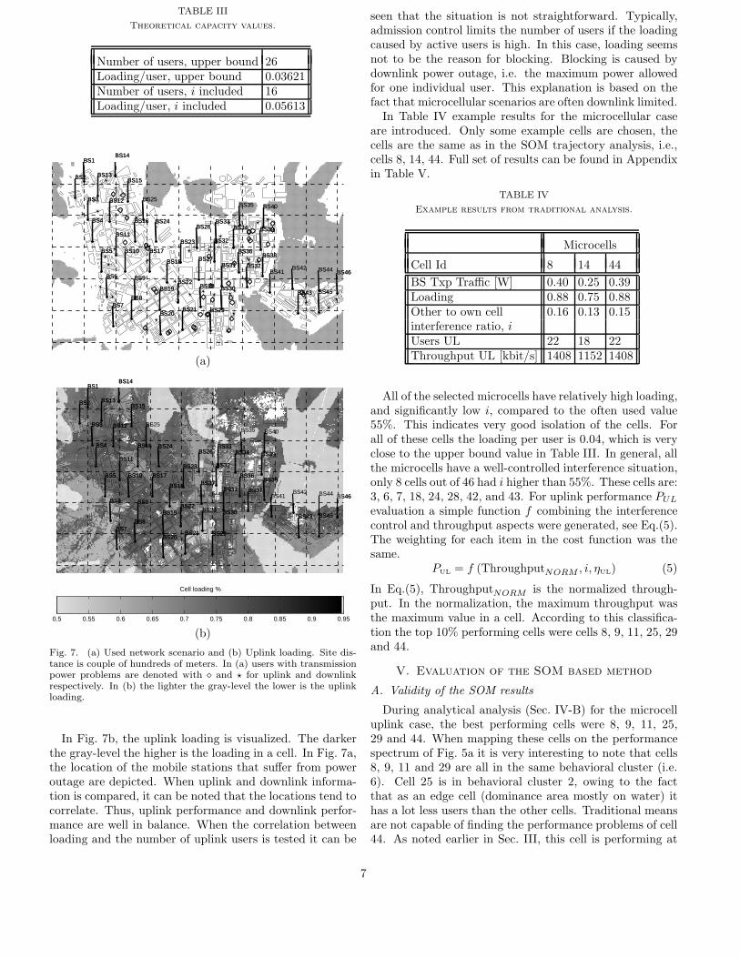
TABLE III

Theoretical capacity values.

Number of users, upper bound 26Loading/user, upper bound 0.03621Number of users, i included 16Loading/user, i included 0.05613

BS1

BS2

BS3

BS4

BS5

BS6

BS7

BS8

BS9

BS10

BS11

BS12

BS13

BS14

BS15

BS16

BS17

BS18

BS19

BS20

BS21

BS22

BS23

BS24

BS25

BS26

BS27

BS28

BS29

BS30

BS31

BS32

BS33

BS34

BS35

BS36

BS37

BS38

BS39

BS40

BS41

BS42

BS43

BS44

BS45

BS46

BS1

BS2

BS3

BS4

BS5

BS6

BS7

BS8

BS9

BS10

BS11

BS12

BS13

BS14

BS15

BS16

BS17

BS18

BS19

BS20

BS21

BS22

BS23

BS24

BS25

BS26

BS27

BS28

BS29

BS30

BS31

BS32

BS33

BS34

BS35

BS36

BS37

BS38

BS39

BS40

BS41

BS42

BS43

BS44

BS45

BS46

(a)

BS1

BS2

BS3

BS4

BS5

BS6

BS7

BS8

BS9

BS10

BS11

BS12

BS13

BS14

BS15

BS16

BS17

BS18

BS19

BS20

BS21

BS22

BS23

BS24

BS25

BS26

BS27

BS28

BS29

BS30

BS31

BS32

BS33

BS34

BS35

BS36

BS37

BS38

BS39

BS40

BS41

BS42

BS43

BS44

BS45

BS46

BS1

BS2

BS3

BS4

BS5

BS6

BS7

BS8

BS9

BS10

BS11

BS12

BS13

BS14

BS15

BS16

BS17

BS18

BS19

BS20

BS21

BS22

BS23

BS24

BS25

BS26

BS27

BS28

BS29

BS30

BS31

BS32

BS33

BS34

BS35

BS36

BS37

BS38

BS39

BS40

BS41

BS42

BS43

BS44

BS45

BS46

Cell loading %

0.5 0.55 0.6 0.65 0.7 0.75 0.8 0.85 0.9 0.95

(b)

Fig. 7. (a) Used network scenario and (b) Uplink loading. Site dis-tance is couple of hundreds of meters. In (a) users with transmissionpower problems are denoted with ⋄ and ⋆ for uplink and downlinkrespectively. In (b) the lighter the gray-level the lower is the uplinkloading.

In Fig. 7b, the uplink loading is visualized. The darkerthe gray-level the higher is the loading in a cell. In Fig. 7a,the location of the mobile stations that suffer from poweroutage are depicted. When uplink and downlink informa-tion is compared, it can be noted that the locations tend tocorrelate. Thus, uplink performance and downlink perfor-mance are well in balance. When the correlation betweenloading and the number of uplink users is tested it can be

seen that the situation is not straightforward. Typically,admission control limits the number of users if the loadingcaused by active users is high. In this case, loading seemsnot to be the reason for blocking. Blocking is caused bydownlink power outage, i.e. the maximum power allowedfor one individual user. This explanation is based on thefact that microcellular scenarios are often downlink limited.

In Table IV example results for the microcellular caseare introduced. Only some example cells are chosen, thecells are the same as in the SOM trajectory analysis, i.e.,cells 8, 14, 44. Full set of results can be found in Appendixin Table V.

TABLE IV

Example results from traditional analysis.

Microcells

Cell Id 8 14 44

BS Txp Traffic [W] 0.40 0.25 0.39Loading 0.88 0.75 0.88Other to own cell 0.16 0.13 0.15interference ratio, iUsers UL 22 18 22Throughput UL [kbit/s] 1408 1152 1408

All of the selected microcells have relatively high loading,and significantly low i, compared to the often used value55%. This indicates very good isolation of the cells. Forall of these cells the loading per user is 0.04, which is veryclose to the upper bound value in Table III. In general, allthe microcells have a well-controlled interference situation,only 8 cells out of 46 had i higher than 55%. These cells are:3, 6, 7, 18, 24, 28, 42, and 43. For uplink performance PUL

evaluation a simple function f combining the interferencecontrol and throughput aspects were generated, see Eq.(5).The weighting for each item in the cost function was thesame.

PUL = f (ThroughputNORM , i, ηUL) (5)

In Eq.(5), ThroughputNORM is the normalized through-put. In the normalization, the maximum throughput wasthe maximum value in a cell. According to this classifica-tion the top 10% performing cells were cells 8, 9, 11, 25, 29and 44.

V. Evaluation of the SOM based method

A. Validity of the SOM results

During analytical analysis (Sec. IV-B) for the microcelluplink case, the best performing cells were 8, 9, 11, 25,29 and 44. When mapping these cells on the performancespectrum of Fig. 5a it is very interesting to note that cells8, 9, 11 and 29 are all in the same behavioral cluster (i.e.6). Cell 25 is in behavioral cluster 2, owing to the factthat as an edge cell (dominance area mostly on water) ithas a lot less users than the other cells. Traditional meansare not capable of finding the performance problems of cell44. As noted earlier in Sec. III, this cell is performing at

7

the edge of its capabilities. Similar results can be foundin the macrocellular and microcellular case when both theuplink and the downlink direction are analyzed [21]. As aconclusion, it can be said that traditional means supportthe conclusions of the cell classification performed by theSOM.

B. Convenience and usability of the SOM based analysis

Current network performance monitoring and analysistools are not capable of meeting the needs and require-ments of service driven networks. The reason for this isthe increasing number of measurements that one shouldprocess simultaneously. The introduction of each new ser-vice or service class will increase the amount of measure-ments the operator needs to collect from the network el-ements. Fig. 8 represents an example of a typical KPIoutput. Each measurement is presented separately and theend user is responsible for correlating the different mea-surements. Furthermore, there is also a physical limitationas to how many measurements can be visualized at once.The end user is responsible for combining the informationfrom different domains.

Fig. 8. An example of measurement visualization in network man-agement system. For each measurement own window is needed.

Current methods rely strongly on averaging or cumulat-ing values over longer period of time, most often one day.KPI values are analyzed as snapshots representing one pe-riod. This approach loses details such as the form of valuedistribution of a KPI inside the period. The approach canbe enhanced by dividing the period into sub-periods andcalculating averages or cumulative sums over those. Thiseasily generates an amount of data so large that details van-ish into them and the simultaneous analysis of KPI combi-nations or performance of cell group becomes even harder.Fig. 9 presents an example of NMS level KPI visualization.The same KPIs are presented with minute, hour and dailyaverage filters. When a problematic KPI is detected, and itis further analyzed, it can happen that the actual behaviorpattern of the cell and its development is not detected atall but the operator ends up optimizing or fixing only oneaspect of the cell’s behavior. This can lead to sub-optimal

solutions that actually disturb the overall quality of thecell.

Fig. 9. Measurement example from NMS with different time reso-lutions. For the data a minute, an hour and daily average filter hasbeen used.

Deriving the QoE from solely objective measurementsrequires advanced intelligence and tools, like the SOM. Themethod proposed in this paper is highly visual and it can beused to combine different types of information like time andgeography with the cell behavior profile. This is differentfrom the traditional analysis where only a few KPIs areanalyzed separately at a time.

C. Scalability of the method

As mentioned earlier, the network performance is cur-rently handled by visualizing the KPIs separately on thescreen. As a result, the number of graphs to be visual-ized increases w.r.t the number of services, the number ofnetwork elements and the number of KPIs used in the anal-ysis. Thus, the optimization of the total performance overa large set of network elements, covering also all of the mostimportant quality aspects, requires the analysis of a largenumber of separate graphs, and the combination of their re-sults to form a single big picture of the current state of thenetwork. However, the number of required visualizationsdoes not increase so radically in the SOM-based approachpresented in this paper. For example, the increase in thenumber of network elements increases only the number ofcell trajectories (as in Fig. 6). If the number of services orthe number of network measurements (variables) increases,the number of component plane visualizations as in Fig. 3also increases. If only the most descriptive combination ofthe single variable rules for each data cluster is shown, thenumber of symbolic rules per data cluster increases withthe number of used variables only if the new set of vari-ables is able to separate the data clusters better than theold set of variables. Thus, the number of rules per clusterdoes not necessarily grow at the same rate as the numberof variables used in the analysis. The SOM-based methodis more scalable with respect to the changes in the problemsetting than the currently used methods.

8

D. Computational complexity of the method

The method consists of two independent algorithms(SOM, k-means) whose computational complexity is depen-dent on the amount of analyzed data. According to [10],the computational complexity of the SOM is proportionalto NMd, where N is the number of data samples in thedata set, M is the number of map units in the SOM and d isthe number of variables (dimension) of the data set. Thus,the training of relatively small SOMs (less than thousandmap units) is computationally efficient even for large datasets. In [13], the computational complexity of the k-meansalgorithm and its application to the clustering of the SOMcodebook vectors is described. The computational com-plexity of the basic k-means clustering algorithm is said tobe proportional to

∑Cmax

k=2 Nk, where N is the number ofdata samples and Cmax is the maximum number of clustersin which the data is to be clustered. However, when the k-means clustering is applied to the codebook vectors of theSOM trained with the data set instead of the original dataset, the computational cost of clustering is reported to re-duce to NM +

∑Cmax

k=2 Mk, thus making it computationallytractable solution for the analysis process described in thispaper. As a reference, the computation time for a singlenetwork scenario was less than an hour, including the basiccomputation, visualization and report generation.

VI. Usage of clustering in optimization

The analysis method presented and used in this articleconsists of two different phases: the clustering of singledata points consisting of several KPIs and clustering of se-quences of these data points. The first phase is actuallythe traditional way to use the SOM. It is able to showwhat types of KPI value combinations there are in general.The basic clustering can be analyzed further in order tosee how an average behavior of cells has developed duringa longer period of time. In the case of behavioral clusters,the method takes into account not only the average behav-ior pattern based on all selected KPIs but also the recentvariation in behavior pattern. By doing this, the methodis able to detect the collapse of an excellent behavior muchearlier than by analyzing only the average behavior. Cellclusters that have been found by the proposed methodscan be used as a starting point for a more detailed analysis.This is especially suitable for trouble shooting type of tasks.For example, in Fig. 10, it can be assumed that the lowerleft corner of the SOM in the upper figure indicates cellsthat have a certain defect. These cells can automaticallybe selected as optimization targets. More detailed analysiscan be provided on them and probably also actions to fixthem can be suggested. The ability to combine the resultprovided by the SOM and the geographical locations of thecells is essential for an operator. The geographical locationinformation can provide support to problem resolution.

The cell clusters can also be used to simplify the taskof parameter provisioning and optimizing. It is not feasi-ble technically nor timewise to optimize the network cellby cell. Cell clustering can be used to increase the oper-ational efficiency of an operator’s tasks. The cells can be

Fig. 10. Example of utilization of cluster information in optimizationprocess. Selection for cells to be optimized/autotuned.

clustered based on their traffic profiles and density, prop-agation conditions, cell types, radio resource managementfunctionality performance etc. When homogeneous mean-ingful groups have been found, all the cells in one group canshare a set of configuration parameter values. This kind ofgrouping based on multiple criteria is more accurate andthe operation of the network will benefit from this: the op-timization process is greatly simplified, improved and madeless error prone and more efficient.

In behavioral clustering, the performance change overtime can be shown on the SOM (see Fig. 6). The methodactually combines two sources of information: change overtime and type of behavior at each separated point of time.This type of analysis can be performed using data averagedover various time periods, ranging from tens of seconds todays. One could, for example, follow one cell movement inthe SOM during peak traffic hours, assuming that networksare able to report cell performance frequently enough.

The sequence clustering method can be applied to followup the optimization actions made in the network. Whenthe network element configuration is changed, the operatornormally wishes to see the effect of the change to perfor-mance. The method can be used to show how the changedcells change their places on the SOM. This kind of infor-

9

mation combination will be essential in the optimizationof WCDMA radio networks. The complexity of the radionetworks is growing as well as the size of networks them-selves. Operators will need means to rapidly analyze thechanges in the network, given the high number of cells, sev-eral services with different QoS criteria and a large amountof collected performance data.

VII. Conclusion

This paper proposes the use of the Self-Organizing Maps(SOM), a neural network method, in the analysis phaseof high level telecommunication network optimization pro-cess. The results provided by the SOM were verified withthe combination of traditional means and expert knowl-edge. It can be stated that the results show a good agree-ment. Being able to understand the SOM results with tra-ditional means increases confidence in the novel analysisand its applicability in the area of cellular networks.

During the course of this work it was noticed that the tra-ditional analysis as such is not adequate enough to provideas enhanced demonstration of the network performance asthe SOM provides. Current performance analysis methodsinclude combinations of planning tool analysis data andreal network measurements. The information format in aplanning tool is a static snapshot of the network situation,and thus, the aspect of time is not present. The KPIs of-fered by the NMS are averaged values. Certain amounts ofinformation of the past behavior of the KPI is also avail-able. In the case of KPI information, no prior knowledgeon the correlation of the different KPIs is available. Thecorrelation analysis and the combination of these two in-formation sources is done manually and it strongly relieson the expertise of the person performing the task.

The strength of the SOM based analysis methods is inthe fact that multiple measurements are used in the anal-ysis at the same time. Furthermore, the output can beprovided in a descriptive format to ease the operator deci-sions. The SOM based application in the analysis of cellularnetworks is not widely spread, and it is worth noting thatthe SOM based analysis has been successfully applied toGSM data to detect anomalous behavior of base stations,see [22] for more details.

In the future, the operation of cellular networks will bestrongly service driven. Compared to the current situationwith provisioning of voice and simple best effort data ser-vices only, the change is enormous. Effective analysis of2G networks’ voice service is currently challenging enoughbecause of large volumes of data collected from networkelements. The evolution towards 3G systems will furtherincrease the amount of data. The operators’ task is to fil-ter the relevant information to a level on which it can beeasily handled. Furthermore, the data set must include allthe essential parts needed to conclude the service quality.Operators can benefit from the introduced neural methodsalready today. The full gain and potential of the advancedanalysis methods can be reached when multiple end-userservices are provided, and the quality perceived by the cus-tomers need to be monitored and optimized.

Acknowledgment

The authors wish to thank Albert Hoglund, Jukka Hen-riksson, Ari Hamalainen, Mikko T. Toivonen, Hannu Mul-timaki and other colleagues from Nokia and Sampsa Lainefrom Helsinki University of Technology for their valuablecomments.

References

[1] Telemanagement Forum, “Enhanced telecom operations mapeTOM, The Business Process Framework for the Informationand Communications Services Industry, Version 3.0,” Tech. Rep.GB921, June 2002.

[2] T. Kohonen, Self-Organizing Maps, Springer-Verlag, Berlin,1995.

[3] K. Raivio, O. Simula, and J. Laiho, “Neural analysis of mo-bile radio access network,” in IEEE International Conferenceon Data Mining, San Jose, California, USA, November 29 - De-cember 2 2001, pp. 457–464.

[4] P. Lehtimaki, K. Raivio, and O. Simula, “Mobile radio accessnetwork monitoring using the self-organizing map,” in Euro-pean Symposium on Artificial Neural Networks, Bruges, Bel-gium, April 24 - 26 2002, pp. 231–236.

[5] T. Kohonen, E. Oja, O. Simula, A. Visa, and J. Kangas, “Engi-neering applications of the self-organizing map,” Proceedings ofthe IEEE, vol. 84, no. 10, pp. 1358–1384, October 1996.

[6] E. Alhoniemi, J. Hollmen, O. Simula, and J. Vesanto, “Processmonitoring and modeling using the self-organizing map,” In-tegrated Computer Aided Engineering, vol. 6, no. 1, pp. 3–14,1999.

[7] O. Simula, P. Vasara, J. Vesanto, and R.-R. Helminen, IndustrialApplications of Neural Networks, chapter The Self-OrganizingMap in Industry Analysis, pp. 87–112, CRC Press, 1999.

[8] O. Simula, J. Ahola, E. Alhoniemi, J. Himberg, and J. Vesanto,“Self-organizing map in analysis of large-scale industrial sys-tems,” in Proceedings of the Workshop on Self-Organizing Maps,Espoo, Finland, July 1 - 3 1999, pp. 375–387, (invited paper).

[9] T. Kohonen, J. Hynninen, J. Kangas, J. Laaksonen, andK. Torkkola, “SOM PAK: The self-organizing map programpackage,” Tech. Rep. A31, Helsinki University of Technology,Laboratory of Computer and Information Science, 1996, Avail-able: http://www.cis.hut.fi/research/som pak/.

[10] J. Vesanto, J. Himberg, E. Alhoniemi, and J. Parhankan-gas, “SOM toolbox for Matlab 5,” Tech. Rep.A57, Helsinki University of Technology, Laboratory ofComputer and Information Science, 2000, Available:http://www.cis.hut.fi/projects/somtoolbox/.

[11] B.S. Everitt, Cluster Analysis, Arnold, 1993.[12] D.L. Davies and D.W. Bouldin, “A cluster separation measure,”

IEEE Transactions on Pattern Analysis and Machine Intelli-gence, vol. 1, no. 2, pp. 224–227, April 1979.

[13] J. Vesanto and E. Alhoniemi, “Clustering of the self-organizingmap,” IEEE Transactions on Neural Networks, vol. 11, no. 3,pp. 586–600, May 2000.

[14] K. Heiska and A. Kangas, “Microcell propagation model fornetwork planning,” in Personal, Indoor and Mobile Radio Com-munications, 1996, vol. 1, pp. 148–152.

[15] J. Rajala, K. Sipila, and K. Heiska, “Predicting in-building cov-erage for microcells and small macrocells,” in IEEE VehicularTechnology Conference, 1999, vol. 1, pp. 180–184.

[16] S. Hamalainen, H. Holma, and K. Sipila, “Advanced WCDMAradio network simulator,” in Personal, Indoor and Mobile RadioCommunications, Osaka, Japan, September 12-15 1999, vol. 2,pp. 951–955.

[17] “Guidelines for evaluation of radio transmission technologies forIMT-2000,” 1997, Recommendation ITU-R M. 1225.

[18] “http://www.3gpp.org/,” .[19] M. Siponen, J. Vesanto, O. Simula, and P. Vasara, “An ap-

proach to automated interpretation of SOM,” in Advances inSelf-Organizing Maps, N. Allinson, H. Yin, L. Allinson, andJ. Slack, Eds. 2001, pp. 89–94, Springer.

[20] J. Laiho, A. Wacker, and T. Novosad, Eds., Radio NetworkPlanning and Optimisation for UMTS, John Wiley & Sons Ltd.,2001.

[21] J. Laiho, K. Raivio, P. Lehtimaki, K. Hatonen, and O. Sim-ula, “Advanced analysis methods for 3G cellular networks,”

10

Tech. Rep. A65, Helsinki University of Technology, Laboratoryof Computer and Information Science, 2002.

[22] A.J. Hoglund, K. Hatonen, and A.S. Sorvari, “A computer host-based user anomaly detection system using the self-organizingmap,” in Proceedings of the International Joint Conference onNeural Networks, 2000, vol. 5, pp. 411–416.

Appendix

11

TABLE V

Results from traditional analysis

Cell Id 1 2 3 4 5 6 7 8 9 10 11 12 13 14 15 16BS Txp 0.39 0.24 0.46 0.56 0.28 0.15 0.15 0.40 0.41 0.23 0.28 0.46 0.32 0.25 0.30 0.24Traffic [W]Loading 0.84 0.72 0.89 0.89 0.70 0.65 0.65 0.88 0.89 0.89 0.89 0.89 0.89 0.75 0.89 0.73Other to own cell 0.32 0.51 0.88 0.20 0.28 0.65 0.59 0.16 0.07 0.29 0.12 0.53 0.28 0.13 0.40 0.32interf. ratio, i

Own cell loading 0.63 0.47 0.47 0.74 0.55 0.39 0.41 0.76 0.83 0.69 0.79 0.58 0.69 0.66 0.64 0.55∆ loading caused by 24 34 47 17 22 40 37 14 7 23 11 35 22 12 29 24other cells [%]Users UL 19 12 16 22 15 11 12 22 25 21 23 17 21 18 19 15Loading/user 0.044 0.060 0.055 0.040 0.047 0.059 0.054 0.040 0.035 0.042 0.039 0.053 0.042 0.042 0.047 0.049Own cell 0.033 0.040 0.029 0.033 0.036 0.035 0.034 0.035 0.033 0.033 0.034 0.034 0.033 0.037 0.033 0.037interf./userThroughput 1216 768 1024 1408 960 704 768 1408 1600 1344 1472 1088 1344 1152 1216 960UL [kbit/s]

Cell Id 17 18 19 20 21 22 23 24 25 26 27 28 29 30 31 32BS Txp 0.32 0.14 0.40 0.38 0.40 0.24 0.39 0.33 0.51 0.21 0.19 0.11 0.37 0.49 0.43 0.14Traffic [W]Loading 0.89 0.70 0.89 0.74 0.76 0.85 0.88 0.89 0.87 0.72 0.81 0.60 0.86 0.87 0.88 0.52Other to own cell 0.23 0.68 0.18 0.27 0.21 0.36 0.19 1.20 0.13 0.39 0.28 0.89 0.12 0.28 0.27 0.46interf. ratio, i

Own cell loading 0.73 0.42 0.76 0.58 0.63 0.62 0.74 0.40 0.77 0.52 0.63 0.32 0.77 0.68 0.69 0.36∆ loading caused by 18 40 15 21 18 27 16 55 12 28 22 47 11 22 21 31other cells [%]Users UL 22 12 22 16 18 18 21 16 22 15 18 9 23 20 21 10Loading/user 0.040 0.058 0.041 0.046 0.042 0.047 0.042 0.056 0.039 0.048 0.045 0.067 0.038 0.044 0.042 0.052Own cell 0.033 0.035 0.034 0.037 0.035 0.035 0.035 0.025 0.035 0.035 0.035 0.035 0.033 0.034 0.033 0.036interf./userThroughput 1408 768 1408 1024 1152 1152 1344 1024 1408 960 1152 576 1472 1280 1344 640UL [kbit/s]

Cell Id 33 34 35 36 37 38 39 40 41 42 43 44 45 46BS Txp 0.38 0.22 0.23 0.28 0.34 0.36 0.22 0.17 0.35 0.12 0.16 0.39 0.29 0.30Traffic [W]Loading 0.72 0.80 0.79 0.89 0.79 0.87 0.68 0.64 0.89 0.46 0.75 0.88 0.77 0.85Other to own cell 0.31 0.26 0.20 0.28 0.53 0.37 0.31 0.51 0.23 0.85 0.63 0.15 0.30 0.21interf. ratio, i

Own cell loading 0.56 0.63 0.66 0.69 0.51 0.63 0.52 0.42 0.73 0.25 0.46 0.76 0.59 0.70∆ loading caused by 23 20 17 22 35 27 24 34 19 46 39 13 23 17other cells [%]Users UL 14 18 19 20 15 18 12 12 22 6 13 22 16 21Loading/user 0.052 0.044 0.042 0.044 0.052 0.048 0.056 0.053 0.041 0.076 0.057 0.040 0.048 0.040Own cell 0.040 0.035 0.035 0.035 0.034 0.035 0.043 0.035 0.033 0.041 0.035 0.035 0.037 0.033interf./userThroughput 896 1152 1216 1280 960 1152 768 768 1408 384 832 1408 1024 1344UL [kbit/s]

12