Aerodynamics and Aeroacoustics Investigation of aLow Speed Subsonic JetPedro R. C. SouzaFederal University of Uberlandia, Block 5P, Uberlandia, Minas Gerais, 38408-100, Brazil

Anderson R. ProencaInstitute of Sound and Vibration Research, Southampton, Hampshire, SO171BJ, UK

Odenir de AlmeidaFederal University of Uberlandia, Block 5P, Uberlandia, Minas Gerais, 38408-100, Brazil

Rodney H. SelfInstitute of Sound and Vibration Research, Southampton, Hampshire, SO171BJ, UK

(Received 1 June 2016; accepted: 5 October 2016)

Low and high speed subsonic jets have been studied in the last 50 years mainly due to their many applications inindustry, such as the discharge of turbojets and turbofan engines. The purpose of this work is to investigate theaerodynamics and the acoustical noise generated by a single stream jet flow operating at low Mach number 0.25and Reynolds number of 2.1×105. The main focus is the flow and acoustical characterization of this low speed jetby applying different experimental techniques for evaluating the velocity field by using measurements with a Pitottube, hot-wire anemometry, and farfield noise acquisition by free field microphones. In order to verify the validityof aeroacoustic predictions for such a low speed jet, a Computational Fluid Dynamics by means of RANS simula-tions via k-ω SST model have been employed coupled with a statistically low-cost Lighthill-Ray-Tracing methodin order to numerically predict the acoustic noise spectrum. The sound pressure level as a function of frequencyis contructed from the experiments and compared with the noise calculations from the acoustic modeling. Thenumerical results for the acoustics and flow fields were well compared with the experimental data, thus showingthat this low-cost flow-acoustic methodology can be used to predict the acoustic noise of subsonic jet flows, evenat low speeds.

NOMENCLATURE

Dj Jet’s diameter [m]

Uj Jet’s velocity [m/s]

M Mach number

k Turbulent kinectic energy [J/kg]

ε Turbulent dissipation rate [J/kgs]

θ Observer’s polar angles [rad]

R Observer’s radius [m]

1. INTRODUCTION

The noise produced by an aircraft has been an important sub-ject in the past few decades in both industry and academic re-search. It is well known that noise is generated by differentcomponents and by the interaction of external flow and the air-craft parts. According to the aircraft performance, during eachphase of flight, one region or piece of equipment should con-tribute more or less to the ”total noise.”1 In other words, theaircraft on the ground, while taxing, is on a run-up from thejet exhaust; during the take-off, it is underneath to departure

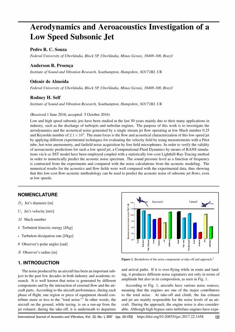
Figure 1. Breakdown of the noise components at take-off and approach.2

and arrival paths. If it is over-flying while in route and land-ing, it produces different noise signatures not only in terms ofamplitude but also in its composition, as seen in Fig. 1.

According to Fig. 1, aircrafts have various noise sources,meaning that the engines are one of the major contributorsto the total noise. At take-off and climb, the fan exhaustand jet are mainly responsible for the noise levels of an air-craft. During the approach, the engine noise is also consider-able. Although high bypass ratio turbofans engines have expe-

International Journal of Acoustics and Vibration, Vol. 22, No. 1, 2017 (pp. 121–130) https://doi.org/10.20855/ijav.2017.22.1458 121

P. R. C. Souza, et al.: AERODYNAMICS AND AEROACOUSTICS INVESTIGATION OF A LOW SPEED SUBSONIC JET

rienced advanced modifications and improvements in the lastfew years, fan noise and jet noise still play the most importantrole in terms of noise generation.2

Driven by new noise regulations and the need to be an en-vironmental less impactant, the aeronautical industry and aca-demic research centers have invested efforts for understand-ing and proposing new techniques and ideas to reduce engineand airframe noise. This subject has undoubtedly proven to bequite important in modern aeronautics and is the main motiva-tion for this work.

The different ways to study engine/airframe noise goes fromseveral experimental techniques up to modern numerical mod-els applied for real articles (engines) or scaled prototypes tobe tested in the laboratory. Experiments often become prohib-ited for real scale since the costs involved are too high, leadingdirectly to experiments with reduced model (scaled models)where knowledge about the problem phenomenology, laws ofsimilarity, and practical equipment is really useful.

On the other hand, the numerical approach is split into atleast three main branches when considering ComputationalFluid Dynamics (CFD):

• Direct Numerical Simulation (DNS) solving all the mo-tion scales of the flow;

• Subgrid Scale (SGS) modeling where LES (Large EddySimulation) is one of the examples, solving partially theflow scales;

• Hybrid or RANS (Reynolds Averaged Navier-Stokes)based methods, including the flow and acoustics analo-gies and empirical models, solving the main characteris-tics of the flow.

Experimental research of free jets has been reported for atleast one century. From the early work of Abramovich3 pass-ing by Towsend,4 Lilley,5 and Lau & Tester,6 among many oth-ers, have found that hot-wire Particle Image Velocimetry (PIV)and modern Laser Doppler (LD) applications have an impor-tant role in turbulent jet measurements, including the case ofjet noise. Measurements made in a low speed air jet (Mach =0.18) with associated cross-spectra and spectral length scalesof the axial and lateral velocity components were performedby Harper-Bourne7 and enhanced by Morris and Zaman,8 thusproviding a more complete picture of the relevant turbulentstatistics, including a wider range of reference points in thejet through cross spectra and cross correlations, second andfourth order statistics, and comparisons with a RANS predic-tion method. Non-intrusive techniques have been employed byMielke et al.9 to measure velocity, density, temperature, andturbulence velocity fluctuations in sparsely seeded, high-speedgas flows, used to make measurements in a 25.4 mm diameterfree jet at subsonic and supersonic flow conditions.

Bridges et al.10 used PIV to calculate turbulence quantitiesin nozzle flows from instantaneous 2D velocity maps. Otherpublished works are related to comparison between experi-mental and numerical results of free turbulent jets. Ghahrema-nian and Moshfegh11 presented numerical results of 3D mod-eling of an isothermal free jet with four different RANS turbu-lence models that were validated against hot-wire anemometrydata. The comparison showed an excellent agreement betweenthe experimental and numerical results.

Other works in the literature show numerical results thatwere validated against proper data or results from others, suchas Freund12 and Stromberg et al.,13 of a simple round jet flowand acoustics. A more specific analysis, including the use ofchevrons, can be seen in the works of Xia et al.,14 Birch et al.,15

and Engel16 among others.In this work, a sequential and comprehensive study about the

physics of a subsonic free stream jet was proposed by perform-ing controlled experiments for the evaluation of the flow andacoustic fields through the use of a multiprobe Pitot tube, hot-wire anemometer, and farfiel acoustic measurements. A com-plementary numerical analysis was adopted by a hybrid ap-proach based on RANS modeling coupled with a noise predic-tion method called Lighthill-Ray-Tracing (LRT) — Silva,17 forfluid flow calculations and the prediction of the sound sourcesin the flow and its propagation to an observer in the far-field,respectively.

By considering such a path, the main contribution of thiswork was to characterize the flow of a low-speed subsonic jet(Mach = 0.25) by means of experimental measurements andto use such data to validate a low-cost hybrid RANS-basedmethod coupled with the LRT method for predicting the far-field noise and its directivity by using the fluid flow propertiescalculated with the RANS technique as input. The experimen-tal data was then used as an original benchmark for the numer-ical prediction tools, which have constituted a low-cost flow-acoustic methodology for being used in industry. The agree-ment between the numerical solution and experimental datawas very good, thus proving that this approach can be used topredict acoustic noise of subsonic jet flows, even at low speeds.

2. EXPERIMENTAL MEASUREMENTS

The experimental part of this research was carried out in theDoak Laboratory, which is a Rolls Royce University Techno-logic Center (UTC) facility located in the Institute of Soundand Vibration Research (ISVR) at University of Souhthamp-ton, United Kingdom. A general description and informationabout this small scale test facility will be given in the sequence.

The ISVR’s Doak laboratory is a 15 m × 7 m × 5 m ane-choic chamber that is fully anechoic down to 400 Hz. Thefour walls, ceiling, and floor are covered with wedge-type ab-sorbent material. A non-forced exhaust system was composedby a rectangular collector section allowing the air flow to passthrough into a small secondary acoustic chamber, as seen inFig. 2. The air flow was fed from two high pressure com-pressed air (20 bar) from two storage tanks and the range ofvelocity available for testing is from Mach 0.2 up to 1. At theseconditions, single jet measurements could be performed onflow regimes characteristic of civil aircrafts. For jet noise mea-surements, both polar and a transversable azimuthal array ofmicrophones were used to give a complete three-dimensionalsound field.

2.1. Test Article Convergent NozzleThe test article used in this work was a 38.1 mm exit-

diameter, convergent, conical nozzle used for most of the testsdone at the Doak Laboratory. This nozzle was selected be-cause its aerodynamic and acoustical characteristics were well-

122 International Journal of Acoustics and Vibration, Vol. 22, No. 1, 2017

P. R. C. Souza, et al.: AERODYNAMICS AND AEROACOUSTICS INVESTIGATION OF A LOW SPEED SUBSONIC JET

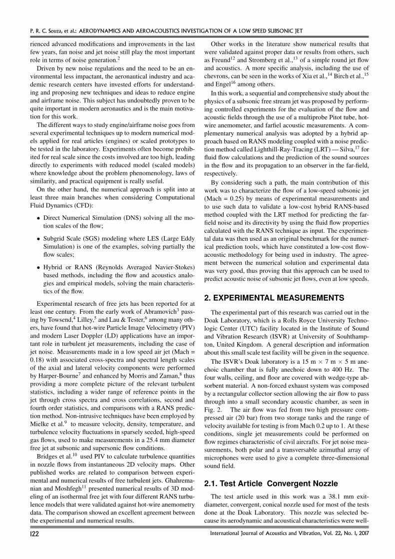
Figure 2. An internal view of the Doak Laboratory ISVR (after Proenca19).

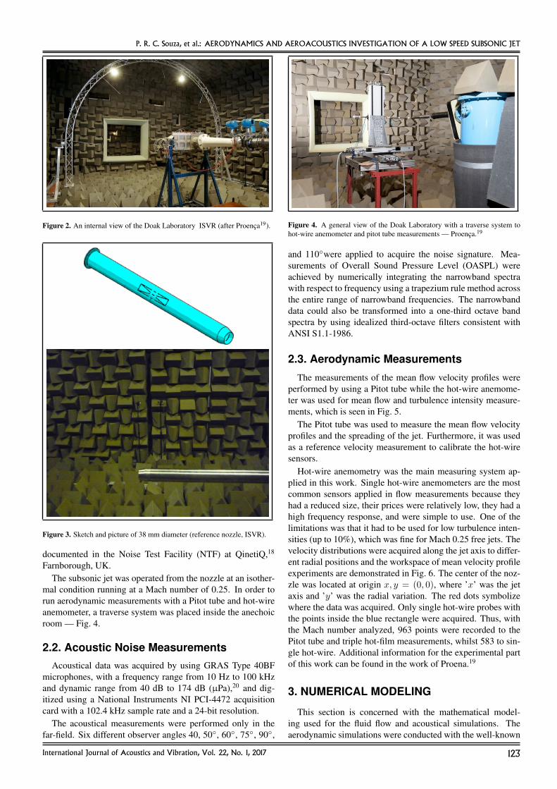
Figure 3. Sketch and picture of 38 mm diameter (reference nozzle, ISVR).

documented in the Noise Test Facility (NTF) at QinetiQ,18

Farnborough, UK.The subsonic jet was operated from the nozzle at an isother-

mal condition running at a Mach number of 0.25. In order torun aerodynamic measurements with a Pitot tube and hot-wireanemometer, a traverse system was placed inside the anechoicroom — Fig. 4.

2.2. Acoustic Noise MeasurementsAcoustical data was acquired by using GRAS Type 40BF

microphones, with a frequency range from 10 Hz to 100 kHzand dynamic range from 40 dB to 174 dB (µPa),20 and dig-itized using a National Instruments NI PCI-4472 acquisitioncard with a 102.4 kHz sample rate and a 24-bit resolution.

The acoustical measurements were performed only in thefar-field. Six different observer angles 40, 50, 60, 75, 90,

Figure 4. A general view of the Doak Laboratory with a traverse system tohot-wire anemometer and pitot tube measurements — Proenca.19

and 110were applied to acquire the noise signature. Mea-surements of Overall Sound Pressure Level (OASPL) wereachieved by numerically integrating the narrowband spectrawith respect to frequency using a trapezium rule method acrossthe entire range of narrowband frequencies. The narrowbanddata could also be transformed into a one-third octave bandspectra by using idealized third-octave filters consistent withANSI S1.1-1986.

2.3. Aerodynamic Measurements

The measurements of the mean flow velocity profiles wereperformed by using a Pitot tube while the hot-wire anemome-ter was used for mean flow and turbulence intensity measure-ments, which is seen in Fig. 5.

The Pitot tube was used to measure the mean flow velocityprofiles and the spreading of the jet. Furthermore, it was usedas a reference velocity measurement to calibrate the hot-wiresensors.

Hot-wire anemometry was the main measuring system ap-plied in this work. Single hot-wire anemometers are the mostcommon sensors applied in flow measurements because theyhad a reduced size, their prices were relatively low, they had ahigh frequency response, and were simple to use. One of thelimitations was that it had to be used for low turbulence inten-sities (up to 10%), which was fine for Mach 0.25 free jets. Thevelocity distributions were acquired along the jet axis to differ-ent radial positions and the workspace of mean velocity profileexperiments are demonstrated in Fig. 6. The center of the noz-zle was located at origin x, y = (0, 0), where ’x’ was the jetaxis and ’y’ was the radial variation. The red dots symbolizewhere the data was acquired. Only single hot-wire probes withthe points inside the blue rectangle were acquired. Thus, withthe Mach number analyzed, 963 points were recorded to thePitot tube and triple hot-film measurements, whilst 583 to sin-gle hot-wire. Additional information for the experimental partof this work can be found in the work of Proena.19

3. NUMERICAL MODELING

This section is concerned with the mathematical model-ing used for the fluid flow and acoustical simulations. Theaerodynamic simulations were conducted with the well-known

International Journal of Acoustics and Vibration, Vol. 22, No. 1, 2017 123

P. R. C. Souza, et al.: AERODYNAMICS AND AEROACOUSTICS INVESTIGATION OF A LOW SPEED SUBSONIC JET

Figure 5. Pitot tubes and single hot-wire sensors — Proenca.19

Figure 6. Acquisition points along the region of the jet for aerodynamic mea-surements — Proenca.19

CFD++ commercial code20 and the acoustical predictions wereobtained using the LRT method.17

3.1. Aerodynamics SimulationA Reynolds Averaged Navier-Stokes (RANS) approach was

used in this work. The compressible steady-state equations ofmotion were solved in a tridimensional domain.

The equation system that described the problem was com-posed by the continuity, Navier-Stokes, and energy equations.Upon using RANS, the term ρu′′i u

′′j that involved the mean of

Table 1. Constants used in the k-ω SST model.

σk1 σk2 σω1 σω2 β1 β2

0.85 1.0 0.5 0.856 0.075 0.0828

γ1 γ2 α1 α2 β∗ κ0.553 0.44 5/9 0.44 0.09 0.41

density and velocity fluctuations appeared and the k-ω SSTturbulence model was used for closure. This model solved thetransport equations for turbulent kinetic energy (k) and spe-cific turbulence dissipation rate (ω), by using the equationspresented below:

ρu′′i u′′j =

2

3δij ρk − µtSij ; (1)

where µt was the turbulent viscosity (Eq. (2)) and Sij wasgiven by Eq. (3).

µtρ

= νt =a1k

max a1ω, SF2, S =

√2SijSijβ∗

; (2)

Sij =

(∂ui∂xj

+∂uj∂xi− 2

3

∂uk∂xk

δij

). (3)

The transport equation for turbulence kinetic energy and thespecific turbulence dissipation rate were:

∂(ρk)

∂t+

∂

∂xj(ρujk) =

∂

∂xj

[(µ+ σkµt)

∂k

∂xj

]+Pk−β∗ρkω;

(4)

∂(ρω)

∂t+

∂

∂xj(ρujω) =

∂

∂xj

[(µ+ σkµt)

∂ω

∂xj

]+γ

νtPk − βρω2

+ 2(1− F1)ρσω21

ω

∂k

∂xj

∂ω

∂xj. (5)

More details about functions such as Pk, Pk, F1, F2, andCDkω can be found in Menter’s21 work. This model, like anyother, brought a large number of empirical constants. Exceptfor constants such as β∗ and κ, all the others had to obey Eq.6;the values used for them in this study are listed in Table 1.

φ = φ1F1 + φ2 (1− F1) ; (6)

where φ is a constant.Several tests were made previously in order to find the best

turbulence model for this problem, although these tests will notbe shown here because they are not the focus of this article.

The governing equations closed with the k-ω SST modelwere solved with a second order accuracy through a Finite Vol-ume formulation. As the jet flow was at Mach lower then 0.3,a preconditioning approach was necessary to stabilize the solu-tion. The final result was obtained when the residual dropped5 orders of magnitude.

3.2. Aeroacoustics PredictionThe sound pressure levels generated by the jet were calcu-

lated by the Lighthill Ray-Tracing method (LRT),17 by usingthe mean flow field characteristics previously calculated by the

124 International Journal of Acoustics and Vibration, Vol. 22, No. 1, 2017

P. R. C. Souza, et al.: AERODYNAMICS AND AEROACOUSTICS INVESTIGATION OF A LOW SPEED SUBSONIC JET

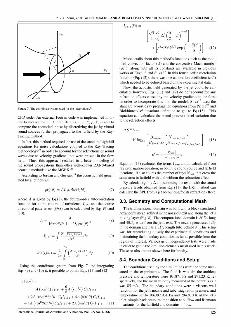
Figure 7. The coordinate system used for the integrations.19

CFD code. An external Fortran code was implemented in or-der to receive the CFD input data as u, c, T , ρ, k, ω and tocompute the acoustical noise by discretizing the jet by virtualsound sources further propagated to the farfield by the Ray-Tracing method.

In fact, this method required the use of the standard Lighthillequations for noise calculations coupled to the Ray-Tracingmethodology22 in order to account for the refractions of soundwaves due to velocity gradients that were present in the flowfield. Thus, this approach resulted in a better modeling ofthe sound propagations than other well-known RANS-basedacoustic methods like the MGBK.23

According to Jordan and Gervais,24 the acoustic field gener-ated by a jet flow is:

p(y, θ) = AIijkldir(ijkl); (7)

where A is given by Eq.(8), the fourth-order autocorrelationfunction for a unit volume of turbulence Iijkl and the sourcedirectional patterns dir(ijkl) can be calculated by Eqs (9) and(10).

A =ρ

16π2c2R2[1−Mc cos(θ)]5 (8)

Iijkl =

∫∂4 (vivjvkvl)

∂τ4d3r (9)

dir(ijkl) =1

2π

2π∫0

(xixjxkxlx4

)dϕ. (10)

Using the coordinate system from Fig. 7 and integratingEqs. (9) and (10) it, it possible to obtain Eqs. (11) and (12):

p (y, θ) =

A(cos4θ

)I1111 +

6

8A(sin4θ

)C1I1111

+ 2A(cos2θsin2θ

)C2I1111 + 4A

(sin4θ

)C3I1111

+ 4A(cos2θsin2θ

)C4I1111 + 2A

(sin4θ

)C5I1111; (11)

I1111(Ω) = [√π

4

c5lα3T

∆2

(3

2− β

)− 132

]

∗[ρ2τ40 Ω4k7/2 exp

(−τ

20 Ω2

8

)]. (12)

More details about this method’s functions such as the mod-ified convection factor (Ω) and the convective Mach number(Mc), along with all its constants are available in previousworks of Engel16 and Silva.17 In this fourth-order correlationfunction (Eq. (12)), there was one calibration coefficient (αT )which needed to be defined based on the experimental data.

Now, the acoustic field generated by the jet could be cal-culated, however, Eqs. (11) and (12) do not account for anyrefraction effects caused by the velocity gradients in the flow.In order to incorporate this into the model, Silva17 used thestandard acoustic ray propagation equations from Pierce22 andBlokhintzev’s25 invariant definition to get to Eq.(13). Thisequation can calculate the sound pressure level variation dueto the refraction effects.

∆SPL =

10 log10

[BsourceBfarfield

[Nray w/ref

Nray w/o ref

]farfield

]; (13)

B =|vray|

(1− uisi)ρc2. (14)

Equation (13) evaluates the terms Vray and si calculated fromray propagation equation, in both the sound source and farfieldlocations. It also counts the number of raysNray that cross thesame area in farfield with and without the refraction effect.

By calculating this ∆ and summing the result with the soundpressure levels obtained from Eq. (11), the LRT method cancalculate the SPL from a jet accounting for its refraction effect.

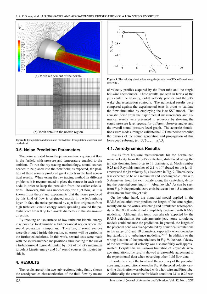
3.3. Geometry and Computational MeshThe tridimensional domain was built with a block structured

hexahedral mesh, refined in the nozzle’s exit and along the jet’smixing layer (Fig. 8). The computational domain is 80Dj longand 40Dj wide from the jet’s exit. The nozzle penetrates 1Dj

in the domain and has a 8Dj length tube behind it. This setupwas for reproducing closely the experimental conditions andmaintaining the boundary condition as far as possible from theregion of interest. Various grid independency tests were madein order to get to the 2 million elements mesh used in this work.These results are not shown here for brevity.

3.4. Boundary Conditions and SetupThe conditions used by the simulations were the same mea-

sured in the experiments. The fluid is was air, the ambientpressure and temperature were 101871 Pa and 291.23 K, re-spectively, and the mean velocity measured at the nozzle’s exitwas 85 m/s. The boundary conditions were a viscous wallfunction for the jet’s nozzle and tube, stagnation pressure, andtemperature set to 106397.931 Pa and 294.870 K at the jet’sinlet, simple back pressure imposition at outflow and Riemanninvariants for the fairfield and domains inflow.

International Journal of Acoustics and Vibration, Vol. 22, No. 1, 2017 125

P. R. C. Souza, et al.: AERODYNAMICS AND AEROACOUSTICS INVESTIGATION OF A LOW SPEED SUBSONIC JET

(a) Mesh refinement of the nozzle.

(b) Mesh detail in the nozzle region.

Figure 8. Computational domain and mesh detail. Computational domain andmesh detail.

3.5. Noise Prediction ParametersThe noise radiated from the jet encounters a quiescent flow

in the farfield with pressure and temperature equaled to theambient. To run the ray tracing methodology, sound sourcesneeded to be placed into the flow field; as expected, the posi-tion of these sources produced great effects in the final acous-tical results. When using the ray tracing method in differentproblems, it is recommended to place the sources in each meshnode in order to keep the precision from the earlier calcula-tions. However, this was unnecessary for a jet flow, as it isknown from theory and experiments that the noise producedby this kind of flow is originated mostly in the jet’s mixinglayer. In fact, the noise generated by a jet flow originates fromhigh turbulent kinetic energy zones spreading around the po-tential core from 0 up to 6 nozzle diameters in the streamwisedirection.

By tracking an iso-surface of low turbulent kinetic energyit is possible to delimitate a tridimensional region where thesound generation is important. Therefore, if sound sourceswere distributed inside this region, no errors will be carried inthe further calculations. In this work, several tests were madewith the source number and positions, thus leading to the use ofa tridimensional region delimited by 10% of the jet’s maximumturbulent kinetic energy and 103 sound sources distributed in-side it.

4. RESULTS

The results are split in two sub-sections, being firstly shownthe aerodynamics characterization of the fluid flow by means

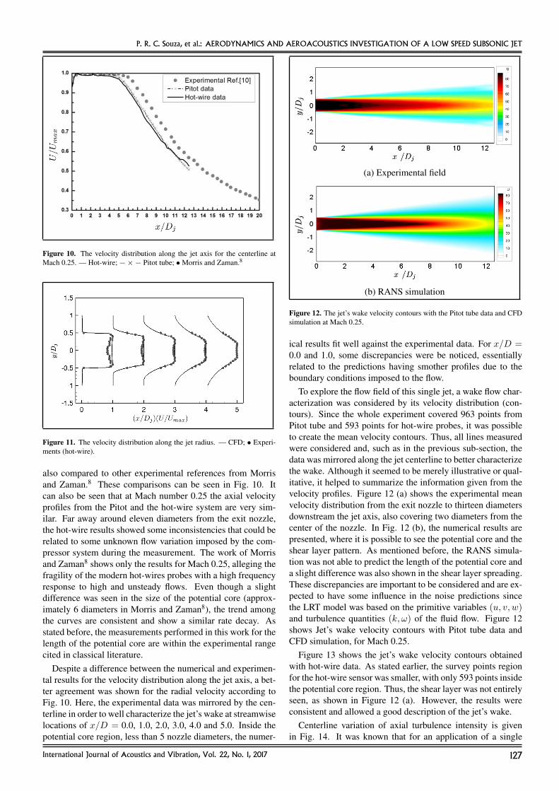
Figure 9. The velocity distribution along the jet axis. — CFD; • Experiments(hot-wire).

of velocity profiles acquired by the Pitot tube and the singlehot-wire anemometer. These results are seen in terms of thejet’s centerline velocity, radial velocity profiles and the jet’swake characterization contours. The numerical results werecompared against the experimental ones in order to validatethe flow simulation by employing the k-ω SST model. Theacoustic noise from the experimental measurements and nu-merical results were presented in sequence by showing thesound pressure level spectra for different observer angles andthe overall sound pressure level graph. The acoustic simula-tions were made aiming to validate the LRT method to describethe physics of the sound generation and propagation of thislow-speed subsonic jet. U/Umax x/Dj

4.1. Aerodynamics ResultsResults from hot-wire measurements for the normalized

mean velocity from the jet’s centerline, distributed along thejet axis domain, from 0 up to 13 diameters, at Mach number0.25 and Reynolds number of 2.1 × 105 (based on the jet di-ameter and the jet velocityUj), is shown in Fig. 9. The velocitywas expected to be at a maximum and unchangeable until 4 to5 diameters from the exit nozzle along the centerline, defin-ing the potential core length — Abramovich.3 As can be seenfrom Fig. 9, the potential core ends between 4 to 4.5 diametersdownstream from the jet axis.

On the other hand, the numerical model applied in theRANS calculation over predicts the length of the core region,mainly due to the vortex-stretching and turbulence heterogene-ity of the 3D flow-field not completely captured with RANSmodeling. Although this trend was already expected by theRANS calculations for axisymmetric jets, some turbulencemodels could enhance the prediction. In general, the length ofthe potential core was over-predicted by numerical simulationsin the range of 6 and 10 diameters, especially when consider-ing standard k-ε turbulence modeling.26, 27 In addition to thewrong location of the potential core in Fig. 9, the rate of decayof the centreline axial velocity was also not fairly well approx-imated. Despite this well-known limitation of Reynolds aver-age simulations, the results showed a reasonable agreement tothe experimental data when observing other fluid flow data.

In order to check the trend and the accuracy of the potentialcore lengths prediction showed in Fig. 9, the axial velocity cen-terline distribution was obtained with a hot-wire and Pitot tube.Additionally, the centerline for Mach conditionM = 0.25 was

126 International Journal of Acoustics and Vibration, Vol. 22, No. 1, 2017

P. R. C. Souza, et al.: AERODYNAMICS AND AEROACOUSTICS INVESTIGATION OF A LOW SPEED SUBSONIC JET

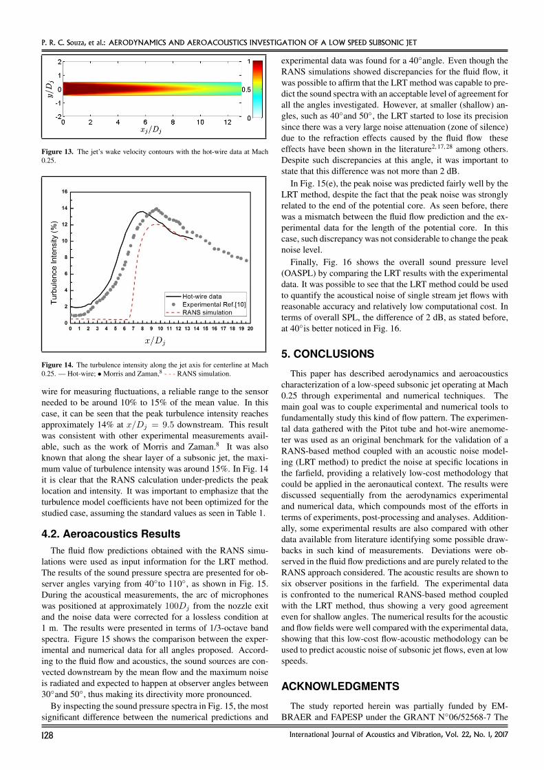
Figure 10. The velocity distribution along the jet axis for the centerline atMach 0.25. — Hot-wire; −×− Pitot tube; • Morris and Zaman.8

Figure 11. The velocity distribution along the jet radius. — CFD; • Experi-ments (hot-wire).

also compared to other experimental references from Morrisand Zaman.8 These comparisons can be seen in Fig. 10. Itcan also be seen that at Mach number 0.25 the axial velocityprofiles from the Pitot and the hot-wire system are very sim-ilar. Far away around eleven diameters from the exit nozzle,the hot-wire results showed some inconsistencies that could berelated to some unknown flow variation imposed by the com-pressor system during the measurement. The work of Morrisand Zaman8 shows only the results for Mach 0.25, alleging thefragility of the modern hot-wires probes with a high frequencyresponse to high and unsteady flows. Even though a slightdifference was seen in the size of the potential core (approx-imately 6 diameters in Morris and Zaman8), the trend amongthe curves are consistent and show a similar rate decay. Asstated before, the measurements performed in this work for thelength of the potential core are within the experimental rangecited in classical literature.

Despite a difference between the numerical and experimen-tal results for the velocity distribution along the jet axis, a bet-ter agreement was shown for the radial velocity according toFig. 10. Here, the experimental data was mirrored by the cen-terline in order to well characterize the jet’s wake at streamwiselocations of x/D = 0.0, 1.0, 2.0, 3.0, 4.0 and 5.0. Inside thepotential core region, less than 5 nozzle diameters, the numer-

(a) Experimental field

(b) RANS simulation

Figure 12. The jet’s wake velocity contours with the Pitot tube data and CFDsimulation at Mach 0.25.

ical results fit well against the experimental data. For x/D =0.0 and 1.0, some discrepancies were be noticed, essentiallyrelated to the predictions having smother profiles due to theboundary conditions imposed to the flow.

To explore the flow field of this single jet, a wake flow char-acterization was considered by its velocity distribution (con-tours). Since the whole experiment covered 963 points fromPitot tube and 593 points for hot-wire probes, it was possibleto create the mean velocity contours. Thus, all lines measuredwere considered and, such as in the previous sub-section, thedata was mirrored along the jet centerline to better characterizethe wake. Although it seemed to be merely illustrative or qual-itative, it helped to summarize the information given from thevelocity profiles. Figure 12 (a) shows the experimental meanvelocity distribution from the exit nozzle to thirteen diametersdownstream the jet axis, also covering two diameters from thecenter of the nozzle. In Fig. 12 (b), the numerical results arepresented, where it is possible to see the potential core and theshear layer pattern. As mentioned before, the RANS simula-tion was not able to predict the length of the potential core anda slight difference was also shown in the shear layer spreading.These discrepancies are important to be considered and are ex-pected to have some influence in the noise predictions sincethe LRT model was based on the primitive variables (u, v, w)and turbulence quantities (k, ω) of the fluid flow. Figure 12shows Jet’s wake velocity contours with Pitot tube data andCFD simulation, for Mach 0.25.

Figure 13 shows the jet’s wake velocity contours obtainedwith hot-wire data. As stated earlier, the survey points regionfor the hot-wire sensor was smaller, with only 593 points insidethe potential core region. Thus, the shear layer was not entirelyseen, as shown in Figure 12 (a). However, the results wereconsistent and allowed a good description of the jet’s wake.

Centerline variation of axial turbulence intensity is givenin Fig. 14. It was known that for an application of a single

International Journal of Acoustics and Vibration, Vol. 22, No. 1, 2017 127

P. R. C. Souza, et al.: AERODYNAMICS AND AEROACOUSTICS INVESTIGATION OF A LOW SPEED SUBSONIC JET

Figure 13. The jet’s wake velocity contours with the hot-wire data at Mach0.25.

Figure 14. The turbulence intensity along the jet axis for centerline at Mach0.25. — Hot-wire; • Morris and Zaman,8 - - - RANS simulation.

wire for measuring fluctuations, a reliable range to the sensorneeded to be around 10% to 15% of the mean value. In thiscase, it can be seen that the peak turbulence intensity reachesapproximately 14% at x/Dj = 9.5 downstream. This resultwas consistent with other experimental measurements avail-able, such as the work of Morris and Zaman.8 It was alsoknown that along the shear layer of a subsonic jet, the maxi-mum value of turbulence intensity was around 15%. In Fig. 14it is clear that the RANS calculation under-predicts the peaklocation and intensity. It was important to emphasize that theturbulence model coefficients have not been optimized for thestudied case, assuming the standard values as seen in Table 1.

4.2. Aeroacoustics ResultsThe fluid flow predictions obtained with the RANS simu-

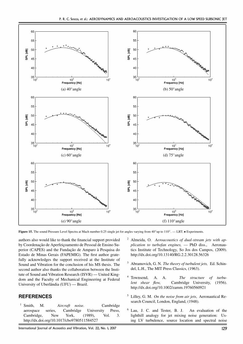
lations were used as input information for the LRT method.The results of the sound pressure spectra are presented for ob-server angles varying from 40to 110, as shown in Fig. 15.During the acoustical measurements, the arc of microphoneswas positioned at approximately 100Dj from the nozzle exitand the noise data were corrected for a lossless condition at1 m. The results were presented in terms of 1/3-octave bandspectra. Figure 15 shows the comparison between the exper-imental and numerical data for all angles proposed. Accord-ing to the fluid flow and acoustics, the sound sources are con-vected downstream by the mean flow and the maximum noiseis radiated and expected to happen at observer angles between30and 50, thus making its directivity more pronounced.

By inspecting the sound pressure spectra in Fig. 15, the mostsignificant difference between the numerical predictions and

experimental data was found for a 40angle. Even though theRANS simulations showed discrepancies for the fluid flow, itwas possible to affirm that the LRT method was capable to pre-dict the sound spectra with an acceptable level of agreement forall the angles investigated. However, at smaller (shallow) an-gles, such as 40and 50, the LRT started to lose its precisionsince there was a very large noise attenuation (zone of silence)due to the refraction effects caused by the fluid flow theseeffects have been shown in the literature2, 17, 28 among others.Despite such discrepancies at this angle, it was important tostate that this difference was not more than 2 dB.

In Fig. 15(e), the peak noise was predicted fairly well by theLRT method, despite the fact that the peak noise was stronglyrelated to the end of the potential core. As seen before, therewas a mismatch between the fluid flow prediction and the ex-perimental data for the length of the potential core. In thiscase, such discrepancy was not considerable to change the peaknoise level.

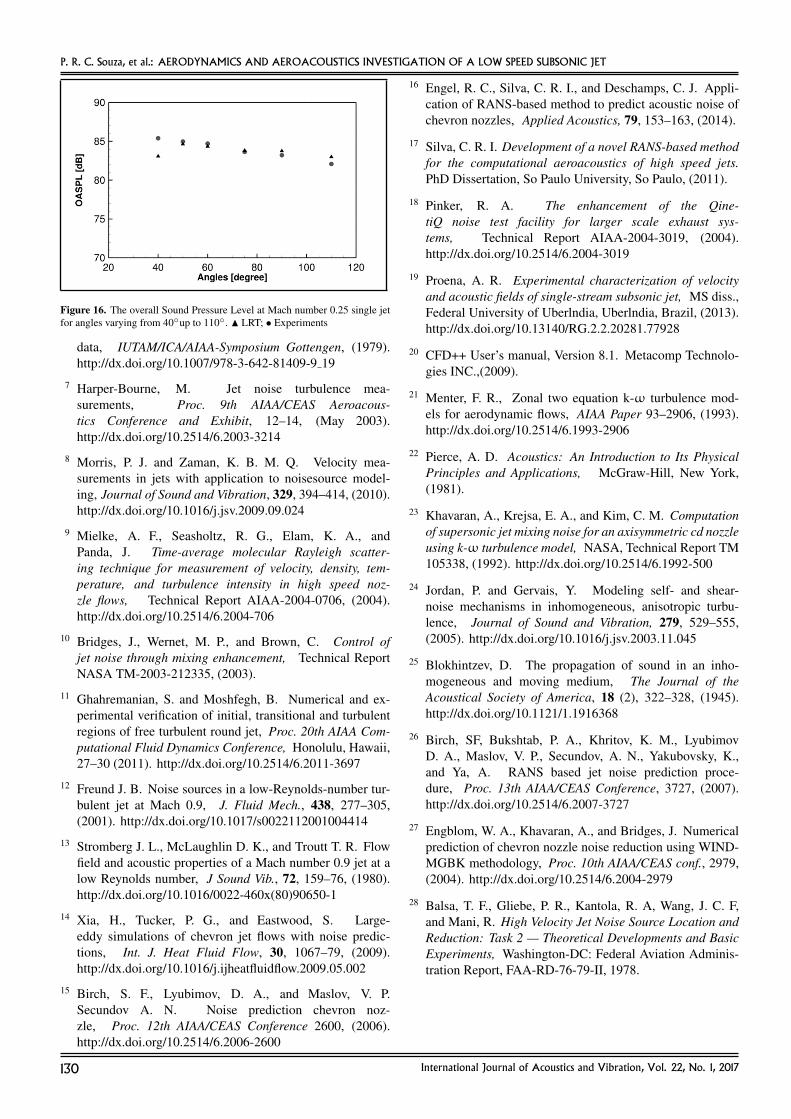
Finally, Fig. 16 shows the overall sound pressure level(OASPL) by comparing the LRT results with the experimentaldata. It was possible to see that the LRT method could be usedto quantify the acoustical noise of single stream jet flows withreasonable accuracy and relatively low computational cost. Interms of overall SPL, the difference of 2 dB, as stated before,at 40is better noticed in Fig. 16.

5. CONCLUSIONS

This paper has described aerodynamics and aeroacousticscharacterization of a low-speed subsonic jet operating at Mach0.25 through experimental and numerical techniques. Themain goal was to couple experimental and numerical tools tofundamentally study this kind of flow pattern. The experimen-tal data gathered with the Pitot tube and hot-wire anemome-ter was used as an original benchmark for the validation of aRANS-based method coupled with an acoustic noise model-ing (LRT method) to predict the noise at specific locations inthe farfield, providing a relatively low-cost methodology thatcould be applied in the aeronautical context. The results werediscussed sequentially from the aerodynamics experimentaland numerical data, which compounds most of the efforts interms of experiments, post-processing and analyses. Addition-ally, some experimental results are also compared with otherdata available from literature identifying some possible draw-backs in such kind of measurements. Deviations were ob-served in the fluid flow predictions and are purely related to theRANS approach considered. The acoustic results are shown tosix observer positions in the farfield. The experimental datais confronted to the numerical RANS-based method coupledwith the LRT method, thus showing a very good agreementeven for shallow angles. The numerical results for the acousticand flow fields were well compared with the experimental data,showing that this low-cost flow-acoustic methodology can beused to predict acoustic noise of subsonic jet flows, even at lowspeeds.

ACKNOWLEDGMENTS

The study reported herein was partially funded by EM-BRAER and FAPESP under the GRANT N06/52568-7 The

128 International Journal of Acoustics and Vibration, Vol. 22, No. 1, 2017

P. R. C. Souza, et al.: AERODYNAMICS AND AEROACOUSTICS INVESTIGATION OF A LOW SPEED SUBSONIC JET

(a) 40angle (b) 50angle

(c) 60angle (d) 75angle

(e) 90angle (f) 110angle

Figure 15. The sound Pressure Level Spectra at Mach number 0.25 single jet for angles varying from 40up to 110. — LRT; • Experiments.

authors also would like to thank the financial support providedby Coordenacao de Aperfeicoamento de Pessoal de Ensino Su-perior (CAPES) and the Fundacao de Amparo a Pesquisa doEstado de Minas Gerais (FAPEMIG). The first author grate-fully acknowledges the support received at the Institute ofSound and Vibration for the conclusion of his MS thesis. Thesecond author also thanks the collaboration between the Insti-tute of Sound and Vibration Research (ISVR) — United King-dom and the Faculty of Mechanical Engineering at FederalUniversity of Uberlandia (UFU) — Brazil.

REFERENCES1 Smith, M. Aircraft noise. Cambridge

aerospace series, Cambridge University Press,Cambridge, New York, (1989), Vol. 3.http://dx.doi.org/10.1017/cbo9780511584527

2 Almeida, O. Aeroacoustics of dual-stream jets with ap-plication to turbofan engines, — PhD diss., Aeronau-tics Institute of Technology, So Jos dos Campos, (2009).http://dx.doi.org/10.13140/RG.2.2.30128.56326

3 Abramovich, G. N. The theory of turbulent jets, Ed. Schin-del, L.H., The MIT Press Classics, (1963).

4 Townsend, A. A. The structure of turbu-lent shear flow, Cambridge University, (1956).http://dx.doi.org/10.1002/zamm.19760560921

5 Lilley, G. M. On the noise from air jets, Aeronautical Re-search Council, London, England, (1948).

6 Lau, J. C. and Tester, B. J. An evaluation of thelighthill analogy for jet mixing noise generation: Us-ing LV turbulence, source location and spectral noise

International Journal of Acoustics and Vibration, Vol. 22, No. 1, 2017 129

P. R. C. Souza, et al.: AERODYNAMICS AND AEROACOUSTICS INVESTIGATION OF A LOW SPEED SUBSONIC JET

Figure 16. The overall Sound Pressure Level at Mach number 0.25 single jetfor angles varying from 40up to 110. N LRT; • Experiments

data, IUTAM/ICA/AIAA-Symposium Gottengen, (1979).http://dx.doi.org/10.1007/978-3-642-81409-9 19

7 Harper-Bourne, M. Jet noise turbulence mea-surements, Proc. 9th AIAA/CEAS Aeroacous-tics Conference and Exhibit, 12–14, (May 2003).http://dx.doi.org/10.2514/6.2003-3214

8 Morris, P. J. and Zaman, K. B. M. Q. Velocity mea-surements in jets with application to noisesource model-ing, Journal of Sound and Vibration, 329, 394–414, (2010).http://dx.doi.org/10.1016/j.jsv.2009.09.024

9 Mielke, A. F., Seasholtz, R. G., Elam, K. A., andPanda, J. Time-average molecular Rayleigh scatter-ing technique for measurement of velocity, density, tem-perature, and turbulence intensity in high speed noz-zle flows, Technical Report AIAA-2004-0706, (2004).http://dx.doi.org/10.2514/6.2004-706

10 Bridges, J., Wernet, M. P., and Brown, C. Control ofjet noise through mixing enhancement, Technical ReportNASA TM-2003-212335, (2003).

11 Ghahremanian, S. and Moshfegh, B. Numerical and ex-perimental verification of initial, transitional and turbulentregions of free turbulent round jet, Proc. 20th AIAA Com-putational Fluid Dynamics Conference, Honolulu, Hawaii,27–30 (2011). http://dx.doi.org/10.2514/6.2011-3697

12 Freund J. B. Noise sources in a low-Reynolds-number tur-bulent jet at Mach 0.9, J. Fluid Mech., 438, 277–305,(2001). http://dx.doi.org/10.1017/s0022112001004414

13 Stromberg J. L., McLaughlin D. K., and Troutt T. R. Flowfield and acoustic properties of a Mach number 0.9 jet at alow Reynolds number, J Sound Vib., 72, 159–76, (1980).http://dx.doi.org/10.1016/0022-460x(80)90650-1

14 Xia, H., Tucker, P. G., and Eastwood, S. Large-eddy simulations of chevron jet flows with noise predic-tions, Int. J. Heat Fluid Flow, 30, 1067–79, (2009).http://dx.doi.org/10.1016/j.ijheatfluidflow.2009.05.002

15 Birch, S. F., Lyubimov, D. A., and Maslov, V. P.Secundov A. N. Noise prediction chevron noz-zle, Proc. 12th AIAA/CEAS Conference 2600, (2006).http://dx.doi.org/10.2514/6.2006-2600

16 Engel, R. C., Silva, C. R. I., and Deschamps, C. J. Appli-cation of RANS-based method to predict acoustic noise ofchevron nozzles, Applied Acoustics, 79, 153–163, (2014).

17 Silva, C. R. I. Development of a novel RANS-based methodfor the computational aeroacoustics of high speed jets.PhD Dissertation, So Paulo University, So Paulo, (2011).

18 Pinker, R. A. The enhancement of the Qine-tiQ noise test facility for larger scale exhaust sys-tems, Technical Report AIAA-2004-3019, (2004).http://dx.doi.org/10.2514/6.2004-3019

19 Proena, A. R. Experimental characterization of velocityand acoustic fields of single-stream subsonic jet, MS diss.,Federal University of Uberlndia, Uberlndia, Brazil, (2013).http://dx.doi.org/10.13140/RG.2.2.20281.77928

20 CFD++ User’s manual, Version 8.1. Metacomp Technolo-gies INC.,(2009).

21 Menter, F. R., Zonal two equation k-ω turbulence mod-els for aerodynamic flows, AIAA Paper 93–2906, (1993).http://dx.doi.org/10.2514/6.1993-2906

22 Pierce, A. D. Acoustics: An Introduction to Its PhysicalPrinciples and Applications, McGraw-Hill, New York,(1981).

23 Khavaran, A., Krejsa, E. A., and Kim, C. M. Computationof supersonic jet mixing noise for an axisymmetric cd nozzleusing k-ω turbulence model, NASA, Technical Report TM105338, (1992). http://dx.doi.org/10.2514/6.1992-500

24 Jordan, P. and Gervais, Y. Modeling self- and shear-noise mechanisms in inhomogeneous, anisotropic turbu-lence, Journal of Sound and Vibration, 279, 529–555,(2005). http://dx.doi.org/10.1016/j.jsv.2003.11.045

25 Blokhintzev, D. The propagation of sound in an inho-mogeneous and moving medium, The Journal of theAcoustical Society of America, 18 (2), 322–328, (1945).http://dx.doi.org/10.1121/1.1916368

26 Birch, SF, Bukshtab, P. A., Khritov, K. M., LyubimovD. A., Maslov, V. P., Secundov, A. N., Yakubovsky, K.,and Ya, A. RANS based jet noise prediction proce-dure, Proc. 13th AIAA/CEAS Conference, 3727, (2007).http://dx.doi.org/10.2514/6.2007-3727

27 Engblom, W. A., Khavaran, A., and Bridges, J. Numericalprediction of chevron nozzle noise reduction using WIND-MGBK methodology, Proc. 10th AIAA/CEAS conf., 2979,(2004). http://dx.doi.org/10.2514/6.2004-2979

28 Balsa, T. F., Gliebe, P. R., Kantola, R. A, Wang, J. C. F,and Mani, R. High Velocity Jet Noise Source Location andReduction: Task 2 — Theoretical Developments and BasicExperiments, Washington-DC: Federal Aviation Adminis-tration Report, FAA-RD-76-79-II, 1978.

130 International Journal of Acoustics and Vibration, Vol. 22, No. 1, 2017