AiMT Advances in Military Technology Vol. 10, No. 2 ...aimt.unob.cz/articles/15_02/04.kumar.pdf · 34 D.V.A.N. Ravi Kumar , S. Koteswara Rao and K. Padma Raju The state equation of

AiMT Advances in Military Technology

Vol. 10, No. 2, December 2015

Underwater Bearings-Only Passive Target Tracking

Using Estimate Fusion Technique

D.V.A.N. Ravi Kumar 1*

, S. Koteswara Rao2 and K. Padma Raju

3

1 Department of Electronics and Communications Engineering, Gayatri Vidya Parishad College

of Engineering for Women , Affiliated to Jawaharlal Nehru Technological University,

Kakinada, India 2 Department of Electrical and Electronics Engineering,

Kalasalingam University, Vijayawada, India

3 Department of Electronics and Communications Engineering,

Jawaharlal Nehru Technological University, Kakinada, India

The manuscript was received on 15 September 2015 and was accepted after revision

for publication on 15 December 2015.

Abstract:

Estimate Fusion Technique (EFT) for Bearings–Only passive target tracking involves

a process of estimating the state of a moving target by fusing the estimates given by

different Nonlinear estimators which are driven by different Bearing measurements

supplied by towed array. The estimates are fused with the help of a Weighted Least

squares Estimator. This novel method has an advantage over the traditional nonlinear

Estimators such as the Extended Kalman Filter (EKF) and Unscented Kalman Filter

(UKF) in terms of estimation errors which is proved in this paper by performing

simulation in Matlab R2009a for a wartime scenario.

Keywords:

Estimate Fusion Technique, Bearings–Only Passive Target Tracking, Towed Array,

Extended Kalman Filter, Unscented Kalman Filter.

1. Introduction

Tracking (a process of estimating the present and future state of a moving target) is an

essential signal processing concept in war environment to remain safe or to blast the foe.

It normally involves estimation of the target motion parameters i.e. range, bearing,

course and velocity with the help of the noisy measurements i.e. range and bearing in

case of active tracking and only bearing in case of passive tracking. Depending on the

* Corresponding author: Department of Electronics and Communications Engineering,

GayatriVidya Parishad College of Engineering for Women, Affiliated to Jawaharlal Nehru

Technological University, Kakinada, India, phone: 918985482118, Email:

[email protected]

32

D.V.A.N. Ravi Kumar , S. Koteswara Rao and K. Padma Raju

relative position of the sensors with respect to the propeller of the observer’s vehicle, the

intensity of the noise in the measurements varies and the measurements can be classified

as hull Mounted and towed array. In detail, if the sensor lies on the body of the ship, it

experiences more noise (because sensor is close to the propeller). These sensors are

termed as hull Mounted sensors (hull meaning body). On the other hand the sensors

which are far from the body of the ship experiences less noise (because sensor is far

from the propellers noise). These sensors are termed as the towed sensors (tow means

drag). In this paper the passive target tracking is done using towed array measurements.

Tracking a target with active sonar measurements,which involves the linear state

and measurement equations is dealt with traditional Kalman filter equations 5.17, 5.18

and 15.19 of [2]. Here the assumption is that the measurement noise in rectangular

coordinates has a mean of zero even after the transformation of measurements from

polar system to rectangular system as shown in [8].The performance of Kalman filter is

improved by precise computation of the mean and covariance of the sensor noise after

the system transformation, followed by subtraction of the calculated mean from the

measurements. This new Kalman filter for active tracking process with the removal of

the bias from the measurements showed a great promise according to results shown

in [8].

Tracking a target with passive measurements, where the measurement equation is

nonlinear is dealt with the conventional nonlinear estimators, such as Extended Kalman

Filter (EKF) in modified polar coordinates. This filter linearizes a nonlinear

measurement equation using the Taylor series expansion [6]. The EKF when applied to

Bearings-Only Tracking (BOT) struggles to perform well occasionally in terms of

convergence of estimation error. This is not acceptable in war environment. The solution

to this problem is given by Modified Gain Extended Kalman Filter (MGEKF) where a

modified gain function in covariance matrix of the state vector is introduced [5].

Uhlman and Juliers Unscented Kalman Filter (UKF) [3], which works on the

principle of unscented transformation of estimate and covariance over a nonlinear

function, made BOT life easier as shown by Kotewara Rao et al. [7]. BOT with towed

array measurements using UKF showed its upper hand over EKF in [4]. Occasionally

some hybrid methods and additional input filters came and showed their importance for

tracking. An example of hybrid method is given in [9] where Pseudo Linear Estimator

(PLE) and MGEKF are combined together to result in a new filter with an improved

performance. [10] shows an example of additional input filters where it is assumed that

the Doppler measurement is also available in addition to range and bearing

measurements.

Recently the particle filter (PF) and its derivatives [1, 2] entered almost all fields

of engineering, like BOT where the estimation is a primary requirement. The popularity

of PF-based algorithms is due to their capability of handling highly nonlinear state and

measurement equations and their ability to deal with any type of noise at the cost of large

computational time and sophisticated processor requirements.

A novel method based on fusion of estimates is proposed in this paper. In this

technique, multiple measurements supplied by different sensors of towed array are

applied to different filters; for example: UKF, which in turn produces different estimates

along with the confidence levels in the estimates. These estimates are fused together

using a weighted least squares estimator to get the final estimate of the state of a moving

target. The block diagram of this approach is shown in Fig. 3. Based on the principle of

operation, this filter can produce improved performance in estimation error over EKF

and UKF as shown in Fig. 1 and less computational cost than PF as shown in Fig. 2.

33



Section 2 deals with the mathematical modelling of a moving target, towed array,

Estimate Fusion technique (EFT), EFT based UKF expressions and at the end, the

performance comparison parameters namely RMS error in position, RMS error in

velocity and Estimator convergence time are defined. Simulation and explanation of

results for a wartime scenario is shown in Section 3 and finally the paper is concluded in

Section 4.

Notation X(aïb) = X(a/b) in the paper = the value of X at time ‘a’ considering the

measurement at time ‘b’.

2. Mathematical Modelling

2.1. Mathematical Modelling of a Moving Target

The components of the position of a target at time ‘k’ in x and y directions are denoted

by x(k), y(k) and the components of the velocity of a target at time ‘k’ in x and y

directions are denoted by )(kvx and )(kvy .State vector as shown in (1) can be

considered for tracking process.

TkvykvxkykxkX )()()()()( (1)

EKF

UKF

EFT-

UKF

PF

ACCURACY

Fig.1 Comparison of the Nonlinear Estimators in Terms of Accuracy.

FILTER

EKF

UKF EFT-

UKF

PF

COMPUTATION

COST

Fig. 2 Comparison of the Nonlinear Estimators in terms of

Computational Cost.

FILTER

34


The state equation of a moving target as per linear, discretized wiener velocity model is

shown in (2)

)()()1( kQKFXKX (2)

F is the state transition matrix=

1000

0100

010

001

T

T

Where T is the time interval between the states, Q(k) is the Gaussian process noise

with a mean zero and a co-variance as given in eqn.13 of [4] is as follows

q

TT

TT

TT

TT

kQkQE T

02/0

002/

2/03/0

02/03/

])()([

2

2

23

23

(3)

Where q is the spectral density of the acceleration errors.

Fig. 3 Block diagram of EFT-UKF

2.2 Mathematical Modelling of Towed Array

Let (x(k), y(k)) be the targets position coordinates at time ‘k’. The towed array is

comprised of two sensors S1 and S2 located at (S1(1), S1(2)), (S2(1), S2(2))

respectively. The azimuth or the bearing at time ‘k’ as viewed at S1and S2 denoted by

B1(k), B2(k) is computed by using the geometry in the Fig. 4.

x(k)-S1(1)

y(k)-S1(2)kB arctan)(1 (4.1)

Y(k) X(K-1/K-1) P(K-1/K-1)

ESTIMATOR-1

X1(K) P1(K) XP-1(K) PP-1(K)

WEIGHTED LEAST SQUARES ESTIMATOR

ym1(k)

𝑿 (𝒌) P(k)

ymp-1(k) X(0/0) P(0/0)

Y(k) X(K-1/K-1) P(K-1/K-1)

ESTIMATOR-P-1 X(K/K) P(K/K)

35



x(k)-S2(1)

y(k)-S2(2)kB arctan)(2 (4.2)

The noise corrupted bearing measurements at S1 and S2 denoted by Bm1(k) and Bm2(k)

are expressed as

(k)+Bn1(k) Bm1(k)=B1 (5.1)

k)+Bn2(k)Bm2(k)=B2( (5.2)

If the measurement vector is considered as

Bm2(k)

Bm1(k)y(k) (6)

The measurement equation can be written as ),k)+v(k)y(k)=h(x(k (7)

The transfer function is denoted by k))h(x(k), and is computed using (8)

x(k)-S2(1)

y(k)-S2(2)arctan

x(k)-S1(1)

y(k)-S1(2)arctan

h(x(k),k)) (8)

(S1(1),S1(2))

(S2(1),S2(2))

(x(k),y(k))

x(k)-S1(1)

x(k)-S2(1)

y(k)-S1(2)

y(k)-S2(2)

Fig 4 Geometry to calculate azimuth or bearing.

B1(k)

B2(k)

36


v(k) in (7) is a sensor noise of type ‘Gaussian’ with a null mean and co-variance R of

the form as shown in (9)

22

21

T ,σσ ]=diagv(k) R=E[ v(k) (9)

Where 22

21 , are the variances of noise in the measurements given by sensors S1 and

S2.

2.3 Estimate Fusion Technique

If sensors which are numbered 1 and j+1 of towed array supply a measurement ymj(k)

using (6). Then yml(k) with l=1, 2... p-1 are the measurements obtained from p elements

of the towed array with the corresponding transfer functions hl(x(k),k) obtained using

(8), covariance matrices Rl obtained using (9). Different UKFs will process these

measurements to produce (kïk)Xl with l=1, 2.... p-1 as estimates with the corresponding

covariance matrices as Pl(kïk). Matrix (kïk)Xl is of the form as shown in (10)

T(n)(2)(1) (kïk)xl..(kïk)xl (kïk)xl(kïk)Xl (10)

The ith

element of the estimate at kth

instant of time considering the kth

measurement

given by the lth

UKF is of the form (kïk)xl (1) . Covariance matrix of the estimate is

denoted by )ï( kkpl and can be expressed in the form of (11)

nplplplkkpl ..21diag)ï( (11)

lip notation in (11) denotes lth

UKFs variance in the estimate of ith

element of its state.

The estimates given by all the p-1 UKFs i.e. ( (kïk)1x (i) (kïk)2x (i) ....... (kïk))1(x (i)p )

are fused to give the consolidated estimate )ï( kkX i . The suffix i indicates the ith

element of the estimate.

(k)l(kïk)X

1

.

.1

1

(kïk)1xp

.

.

(kïk)x2

(kïk)x1

ii

1)x1(p(i)

(i)

(i)

(12)

)(kli is Gaussian noise of dimensions (p-1)x1, mean of zero and covariance R(i). It is the

error in ith

element of the estimate.

)p..pp(R 1)i(p2i1i(i) diag (13)

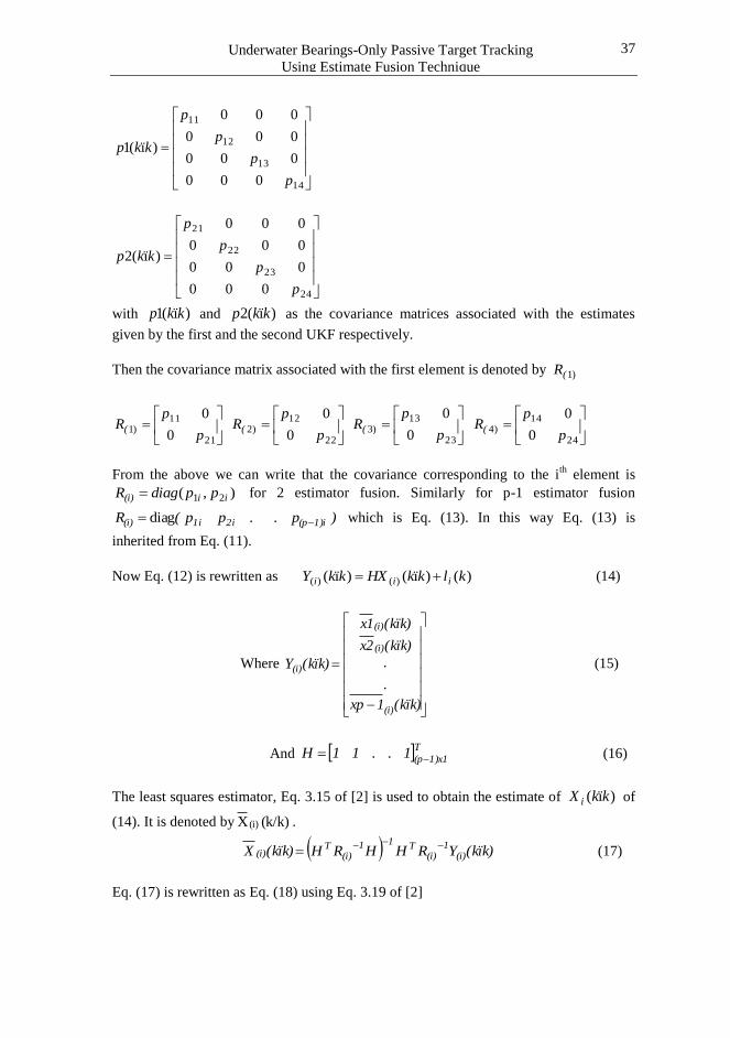
Eq. (13) is inherited from Eq. (11) as follows

If we are trying to fuse two estimator outputs with four elements in the state vector. Then

(11) will be in the form of

37



14

13

12

11

000

000

000

000

)ï(1

p

p

p

p

kkp

24

23

22

21

000

000

000

000

)ï(2

p

p

p

p

kkp

with )ï(1 kkp and )ï(2 kkp as the covariance matrices associated with the estimates

given by the first and the second UKF respectively.

Then the covariance matrix associated with the first element is denoted by )1(R

21

11)1

0

0

p

pR(

22

12)2

0

0

p

pR(

23

13)3

0

0

p

pR(

24

14)4

0

0

p

pR(

From the above we can write that the covariance corresponding to the ith

element is

),( 21 ii(i) ppdiagR for 2 estimator fusion. Similarly for p-1 estimator fusion

)p..pp(R 1)i(p2i1i(i) diag which is Eq. (13). In this way Eq. (13) is

inherited from Eq. (11).

Now Eq. (12) is rewritten as )()ï()ï( )()( klkkHXkkY iii (14)

Where

(kïk)1xp

.

.

(kïk)x2

(kïk)x1

(kïk)Y

(i)

(i)

(i)

(i) (15)

And T 1)x1(p1..11H (16)

The least squares estimator, Eq. 3.15 of [2] is used to obtain the estimate of )ï( kkX i of

(14). It is denoted by (k/k)X (i) .

(kïk)YRHHRH(kïk)X (i)1

(i)T11

(i)T

(i)

(17)

Eq. (17) is rewritten as Eq. (18) using Eq. 3.19 of [2]

38


1p

1j2ji

(i)

11p

1j2ji

(i)

p

(kïk)Xj

p

1(kïk)X (18)

The fusion-based estimate taking kth

measurement into consideration denoted by

(k/k)X is composed using (18)

T(n)(2)(1) (kïk)x..(kïk)x(kïk)x(kïk)X (19)

The covariance in the fused- estimate is as follows

1p

1i

Pi(kïk)1p

1P(kïk) (20)

2.4 Estimate Fusion Technique based UKF( EFT-UKF) Equations

Identify the state vector X(k) of n elements. Then the state equation expressed in the

form of (21) and measurement equation in the form of (22) are derived.

State equation: )()()1( kwkFXkX (21)

Measurement equation: )()),(()( kvkkxhkym ),0(~)( Qkw ),0(~)( Rkv (22)

There after the initialization of EFT-UKF is performed, which involves the initialization

of state as shown in (23) and initialization of the covariance as shown in (24).

)]0([)0ï0( XEX (23)

]))0ï0())(0ï0([()0ï0( TXXXXEP (24)

As the state equation is linear in nature,a priori estimate of the state and the covariance

are computed using the prediction step of normal kalman filter.

)1ï1()1ï( kkXFkkX (25)

QFkkFPkkP T )1ï()1ï( (26)

Correction step starts with the computation of 2n+1 sigma points using the following

)1ï()(0 kkXKX

nikkPnkkXKXT

rowi

ith .....3,2,1)1ï()()1ï()(

nikkPnkkXKXT

rowi

inth .....3,2,1)1ï()()1ï()( (27)

Where is a scaling parameter given by

nkan )(2

39



The weights corresponding to the sigma points are computed using the following

relations

nwm

0

20 1

nwc

nin

wim 2.....2,1

)(2

1

nin

wic 2.....2,1

)(2

1

(28)

Where , and ka are the parameters used in the algorithm.

The 2n+1 sigma points are transformed over the nonlinear measurement equation i.e.

Eq. (22)

)),(()( kkxhkym ii .2.....3,2,1 ni (29)

A posterior estimate computation starts by taking the weighted average of the

transformed sigma points as given below

n

i

iim kymwkmy

2

0

)()( )()( (30)

variances corresponding to the a posterior estimate denoted by yP is computed

according to Eq. 14.65 of [2] as follows

RkmykymkmykymwPTi

n

i

iicy

)()()()(2

0

)( (31)

Crosscovariances of the a posterior estimate denoted by xyP is computed according to

Eq. 14.66 of [2] as follows.

Tin

i

iicxy kmykymkkXkXwP )()()1ï()(

2

0

)()(

(32)

The Kalman gain kk is calculated using Eq. 14.67 of [2] as follows

1

yxy PPkk (33)

Finally the a posterior estimate denoted by )ï( kkX is computed according to Eq. 14.67

of [2] as follows.

40


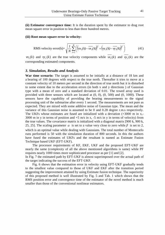
))()(()1ï()ï( kmykymkkkkXkkX (34)

Covariance matrix corresponding to the a posterior estimate denoted by )ï( kkP is

computed according to Eq. 14.67 of [2] as follows.

T

y kkPkkkkPkkP )()()1ï()ï( (35)

Equations (23) to (35) are the UKF equations applied for all the p-1 measurements

(ymj(k) j=1,2,…p-1) obtained from the sensors of the towed array to produce )/( kkjX ,

)/( kkPj with j=1,2,……p-1 as the aposterior estimates and covariances respectively

using the corresponding transfer functions hj(x(k),k). The least squares estimator is used

to fuse all the p-1 estimates to give (kïk)X , as fused estimate with )/( kkP as the

corresponding covariance matrix.

The fused estimate is composed of n elements as follows

T(n)(2)(1) (kïk)x..(kïk)x(kïk)x(kïk)X (36)

Where the ith

element of the fused estimate is derived in estimate fusion technique i.e.

section 2(c) and is shown below in (37)

1p

1j2ji

(i)

11p

1j2ji

(i)

p

(kïk)Xj

p

1(kïk)X (37)

If we assume all the weights are equal, then the fused estimate can be written as

1p

0i

i(kïk)X1p

1(kïk)X (38)

The related covariance matrix is given below

1

1

)ï(1

1)ï(

p

i

kkPip

kkP (39)

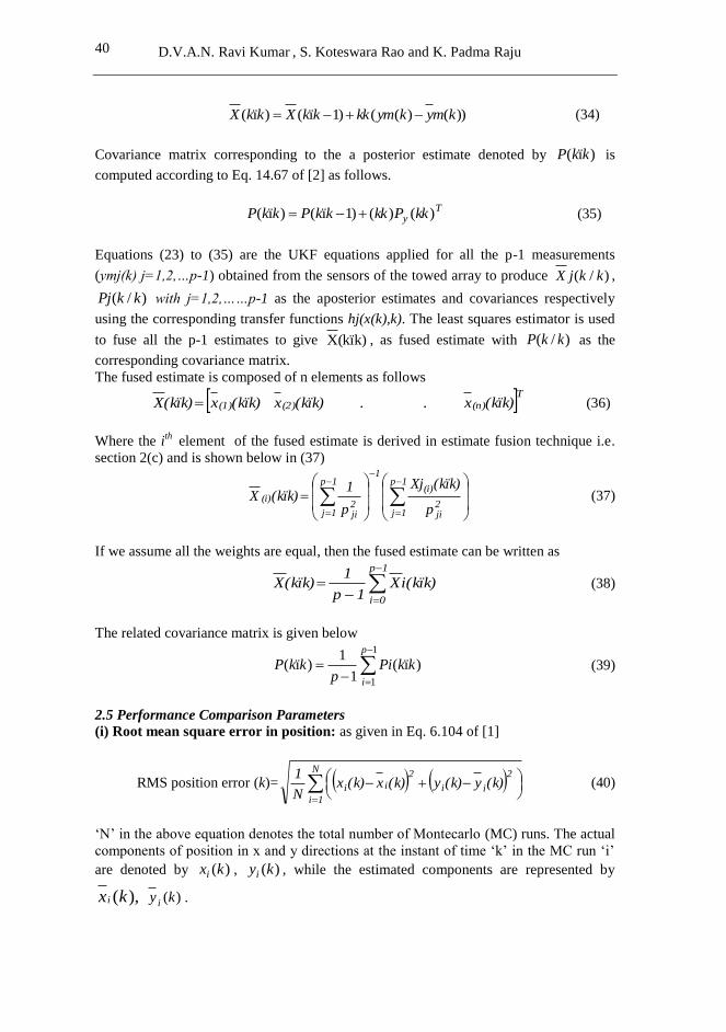
2.5 Performance Comparison Parameters

(i) Root mean square error in position: as given in Eq. 6.104 of [1]

RMS position error (k)=

N

1i

2

ii

2

ii (k)y(k)y(k)x(k)xN

1 (40)

‘N’ in the above equation denotes the total number of Montecarlo (MC) runs. The actual

components of position in x and y directions at the instant of time ‘k’ in the MC run ‘i’

are denoted by )(kxi , )(kyi , while the estimated components are represented by

),(kxi )(ky i .

41



(ii) Estimator convergence time: It is the duration spent by the estimator to drag root

mean square error in position to less than three hundred metres.

(iii) Root mean square error in velocity:

RMS velocity error(k)=

N

1i

2

ii

2

ii (k)vy(k)vy(k)vx(k)vxN

1 (41)

)(kvxi and )(kvy i are the true velocity components while )(kvxi and )(kvy i are the

corresponding estimated components.

3. Simulation, Results and Analysis

War time scenario: The target is assumed to be initially at a distance of 18 km and

a bearing of 100 degrees with respect to the true north. Thereafter it tries to move at a

constant velocity of 10 meters per second in the direction of true north but it is disturbed

to some extent due to the acceleration errors (in both x and y directions ) of Gaussian

type with a mean of zero and a standard deviation of 0.01. The towed array used is

provided with three sensors which are located at (0, 0), (0, 500) and (0, 1000). These

sensors have the capability of providing the bearing measurements to the signal

processing unit of the submarine after every 1 second. The measurements are not pure as

expected. They are mixed with some additive noise of Gaussian type. The mean and the

variance of this Gaussian noise is assumed to be 0 and 0.28 degree r.m.s respectively.

The UKFs whose estimates are fused are initialized with a deviation (+3000 m in x,-

3000 m in y in terms of position and +5 m/s in x, -5 m/s in y in terms of velocity) from

the true values. The covariance matrix is initialized with a diagonal matrix [900 k, 900 k,

25, 25]. The scaling parameter is set to a value very close to zero while is set to 2,

which is an optimal value while dealing with Gaussians. The total number of Montecarlo

runs performed is 50 with the simulation duration of 800 seconds. In this the authors

have fused the estimates of UKFs and the resultant is named as Estimate Fusion

Technique based UKF (EFT-UKF).

The processor requirements of KF, EKF, UKF and the proposed EFT-UKF are

nearly the same (complexity of all the above mentioned algorithms is same) while PF

requires nearly 1000 times more sophisticated processor as per [1] and [2].

In Fig. 7 the estimated path by EFT-UKF is almost superimposed over the actual path of

the target indicating the success of the EFT-UKF.

Fig. 6 shows that the estimation error in velocity using EFT-UKF gradually tends

to the smallest value compared to those of UKF and EKF after the transition period

suggesting the improvement attained by using Estimate fusion technique. The superiority

of this proposed method is well illustrated by Fig. 5 and Tab. 1 which shows that the

RMS position error and convergence time of the estimator of the novel method is much

smaller than those of the conventional nonlinear estimators.

42


Fig. 5 Comparison of RMS position errors

Fig. 6 Comparison of RMS velocity errors

0 100 200 300 400 500 600 700 8000

500

1000

1500

2000

2500

3000

3500

4000

4500RMS error in position vs time graph

TIME(in sec)

RM

S p

ositio

n e

rror(

mete

rs)

UKF

EFT-UKF

EKF

0 100 200 300 400 500 600 700 8000

1

2

3

4

5

6

7

8RMS error in velocity vs time graph

TIME(sec)

RM

S v

elo

city e

rror(

mete

rs/s

econd)

UKF

EFT-UKF

EKF

43



Fig. 7 Actual path and estimated path provided by EFT-UKF

Tab. 1 Comparison table of nonlinear Estimators

Filter RMS position error (m) RMSE velocity

error (m/s)

Estimator

Convergence

Time(s)

EKF 194 0.457 606

UKF 194 0.424 583

EFT-UKF 108 0.353 343

4. CONCLUSIONS

EFT based UKF has a superior performance over the conventional nonlinear estimators

such as EKF and UKF in terms of the estimation errors in position and velocity and at

the same time it needs less computational requirements than PF which suggests that, the

estimate fusion technique can provide an optimal solution for tracking a moving target in

passive mode. The performance of all the existing nonlinear estimators can be sent to

a new level by employing the EFT.

ACKNOWLEDGEMENT

Authors would like to thank the management, Gayatri Vidya Parishad College of

Engineering for Women, Madhurawada, Visakhapatnam, India for their support in

smooth completion of this work. Last but not least authors would also like to thank the

reviewers and the staff of AiMT who have given valuable suggestions to make the article

more valuable.

0 2000 4000 6000 8000 10000 12000-20000

-15000

-10000

-5000

0

5000

x (meters)

y (m

eter

s)

REAL AND ESTIMATED PATHS

Actual path

SENSOR 1

SENSOR 2

SENSOR 3

estimated path by EFT-UKF

44


REFERENCES

[1] RISTICK, B., ARULAMPALEM, S. and GORDON, N. Beyond the Kalman

Filter–Particle Filters for Tracking Applications, Artech House, DSTO, 2004. p.

129.

[2] SIMON, D. Optimal State Estimation: Kalman, H , and Nonlinear Approaches,

Wiley-Interscience, 2006, p. 83,128,129.

[3] JULIER, S. and UHLMANN, J. Unscented Filtering and Nonlinear Estimation ,

Proceedings of the IEEE, 2004, vol. 92, no. 3, p. 401-422.

[4] ZHANG, H., DAI, G., SUN, J. and ZHAO , Y. Unscented Kalman filter and its

nonlinear application for tracking a moving target, Optik, 2013, vol. 124, p. 4468-

4471.

[5] SONG, T.L. and SPEYER, J.L. A Stochastic Analysis of a Modified Gain

Extended Kalman Filter with Applications to estimation with Bearings-only

measurements, IEEE Trans. Automat. Contr., 1985, vol. 30, no. 10, p. 940-949.

[6] AIDALA, V.J. and HAMMEL, S.E. Utilization of modified polar coordinates for

bearings only tracking, IEEE Trans. Automatic Control , 1983, vol.28, no. 3, p.

283-294.

[7] KOTESWARA RAO, S., RAJA RAJESWARI, K. and LINGAMURTY, K.S.

Unscented Kalman Filter with Application to Bearings-Only Target Tracking, IETE

journal of research , 2009, vol. 55, no. 2, p. 63-67.

[8] LERRO, D. and BAR-SHALOM, Y. Tracking With Debiased Consistent

Converted Measurements Versus EKF, IEEE transactions on aerospace and

electronic systems , 1993, vol. 29, no. 3, pp. 1015-1022.

[9] RAO, S.K., KUMAR, D.V.A.N.R. and RAJU, K.P. Combination of Pseudo Linear

Estimator and modified gain bearings-only extended Kalman filter for passive

target tracking in abnormal conditions, Ocean Electronics (SYMPOL), 2013, p. 3-8.

[10] ZHOU, G., PELLETIER, M., KIRUBARAJAN T. and QUAN, T. Statically Fused

Converted Position and Doppler Measurement Kalman Filters, Aerospace and

Electronic Systems, IEEE Transactions on, 2014, Vol. 50, no. 1, p. 300-318.

Documents

AiMT Advances in Military Technology Vol. 10, No. 2 ...aimt.unob.cz/articles/15_02/04.kumar.pdf · 34 D.V.A.N. Ravi Kumar , S. Koteswara Rao and K. Padma Raju The state equation of