An Efficient Unification Algorithm - nsl.com · An Efficient Unification Algorithm 259 Resolution, however, is not the only application of the unification algorithm. In fact, its

An Efficient Unification Algorithm

ALBERTO MARTELLI

Consiglio Nazionale delle Ricerche

and

UGO MONTANARI

Universita di Pisa

The unification problem in f'mst-order predicate calculus is described in general terms as the solution of a system of equations, and a nondeterministic algorithm is given. A new unification algorithm, characterized by having the acyclicity test efficiently embedded into it, is derived from the nondeterministic one, and a PASCAL implementation is given. A comparison with other well-known unification algorithms shows that the algorithm described here performs well in all cases.

Categories and Subject Descriptors: F.2.2 [Analysis of Algori thms and Problem Complexity]: Nonnumerical Algorithms and Problems--complexity of proof procedures; F.4.1 [Mathematical Logic and Formal Languages]: Mathematical Logic--mechanical theorem proving; 1.2.3 [Artifi- cial Intelligence]: Deduction and Theorem Proving--resolution

General Terms: Algorithms, Languages, Performance, Theory

1. INTRODUCTION

I n i ts essence , t h e un i f i c a t i on p r o b l e m in f i r s t - o r d e r logic c a n be e x p r e s s e d as fol lows: G i v e n two t e r m s c o n t a i n i n g s o m e va r i ab le s , f ind, i f i t exis ts , t h e s i m p l e s t s u b s t i t u t i o n (i.e., a n a s s i g n m e n t of s o m e t e r m to e v e r y va r i ab l e ) w h i c h m a k e s t h e two t e r m s equa l . T h e r e s u l t i n g s u b s t i t u t i o n is ca l l ed t h e most general unifier a n d is u n i q u e u p to v a r i a b l e r e n a m i n g .

U n i f i c a t i o n was f i rs t i n t r o d u c e d b y R o b i n s o n [17, 18] as t h e c e n t r a l s t e p of t h e i n fe rence ru l e ca l l ed r e so lu t ion . T h i s s ingle, p o w e r f u l ru le c a n r e p l a c e a l l t h e a x i o m s a n d in fe rence ru les of t h e f i r s t - o r d e r p r e d i c a t e ca l cu lus a n d t h u s was i m m e d i a t e l y r e cogn i zed as e spec i a l l y s u i t e d to m e c h a n i c a l t h e o r e m p rove r s . I n fact , a n u m b e r of s y s t e m s b a s e d on r e s o l u t i o n we re b u i l t a n d t r i e d on a v a r i e t y of d i f f e r en t a p p l i c a t i o n s [5]. E v e n t h o u g h f u r t h e r r e s e a r c h m a d e i t a p p a r e n t t h a t r e s o l u t i o n s y s t e m s a re d i f f icu l t to d i r e c t d u r i n g p r o o f s e a r c h a n d t h u s a r e o f t en p r o n e to c o m b i n a t o r i a l exp los ion [6], new i m p e t u s to t h e r e s e a r c h in t h i s a r e a was g iven b y K o w a l s k i ' s i d e a of i n t e r p r e t i n g p r e d i c a t e logic as a p r o g r a m m i n g l a n g u a g e [10]. H e r e p r e d i c a t e logic c l auses a r e s een as p r o c e d u r e de c l a r a t i ons , a n d p r o c e d u r e i n v o c a t i o n r e p r e s e n t s a r e s o l u t i o n s tep . F r o m th i s v i ewpo in t , t h e o r e m p r o v e r s can be r e g a r d e d as i n t e r p r e t e r s for p r o g r a m s w r i t t e n in p r e d i c a t e logic, a n d th i s a n a l o g y sugges t s e f f ic ien t i m p l e m e n t a t i o n s [3, 25].

Authors' present addresses: A. Martelli, Istituto di Scienze della Informazione, Universit~ di Torino, Corso M. d'Azeglio 42, 1-10125 Torino, Italy; U. Montanari, Istituto di Scienze della Informazione, Universit& di Pisa, Corso Italia 40, 1-56100 Pisa, Italy. Permission to copy without fee all or part of this material is granted provided that the copies are not made or distributed for direct commercial advantage, the ACM copyright notice and the title of the publication and its date appear, and notice is given that copying is by permission of the Association for Computing Machinery. To copy otherwise, or to republish, requires a fee and/or specific permission. © 1982 ACM 0164-0925/82/0400-0258 $00.75

ACM Transactions on Programming Languages and Systems, Vol. 4, No. 2, April 1982, Pages 258-282.

An Efficient Unification Algorithm 259

Resolution, however, is not the only application of the unification algorithm. In fact, its pattern matching nature can be exploited in many cases where symbolic expressions are dealt with, such as, for instance, in interpreters for equation languages [4, 11], in systems using a database organized in terms of productions [19], in type checkers for programming languages with a complex type structure [14], and in the computation of critical pairs for term rewriting systems [9].

The unification algorithm constitutes the heart of all the applications listed above, and thus its performance affects in a crucial way the global efficiency of each. The unification algorithm as originally proposed can be extremely ineffi- cient; therefore, many attempts have been made to find more efficient algorithms [2, 7, 13, 15, 16, 22]. Unification algorithms have also been extended to the case of higher order logic [8] and to deal directly with associativity and commutativity [20]. The problem was also tackled from a computational complexity point of view, and linear algorithms were proposed independently by Martelli and Mon- tanari [13] and Paterson and Wegman [15].

In the next section we give some basic definitions by representing the unification problem as the solution of a system of equations. A nondeterministic algorithm, which comprehends as special cases most known algorithms, is then defined and proved correct. In Section 3 we present a new version of this algorithm obtained by grouping together all equations with some member in common, and we derive from it a first version of our unification algorithm.

In Sections 4 and 5 we present the main ideas which make the algorithm efficient, and the last details are described in Section 6 by means of a PASCAL implementation.

Finally, in Section 7, the performance of this algorithm is compared with that of two well-known algorithms, Huet's [7] and Paterson and Wegman's [15]. This analysis shows that our algorithm has uniformly good performance for all classes of data considered.

2. UNIFICATION AS THE SOLUTION OF A SET OF EQUATIONS: A NONDETERMINISTIC ALGORITHM

In this section we introduce the basic definitions and give a few theorems which are useful in proving the correctness of the algorithms. Our ay of stating the unification problem is slightly more general than the classical one due to Robinson [18] and directly suggests a number of possible solution methods.

Let

A = U Ai (Ai A A j = O, i # j ) i=0,1 ....

be a ranked alphabet, where A~ contains the i-adic function symbols (the elements of A0 are constant symbols). Furthermore, let V be the alphabet of the variables. The terms are defined recursively as follows:

(1) constant symbols and variables are terms; (2) if tl . . . . . tn (n >_ 1) are terms and f E A,, then f ( 6 , . . . , tn) is a term.

A subst i tut ion t~ is a mapping from variables to terms, with v~(x) = x almost everywhere. A substitution can be represented by a finite set of ordered pairs

ACM Transact ions on Programming Languages and Systems, Vol. 4, No. 2, April 1982.

260 A. Martelli and U. Montanari

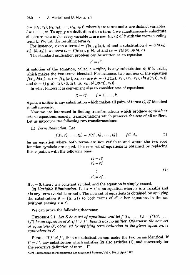
# = {(t,, xl), (t2, x 2 ) , . . . , (tm, Xm)} where ti are terms and xi are distinct variables, i = 1 , . . . , m. To apply a substi tut ion # to a te rm t, we simultaneously subst i tute all occurrences in t of every variable xi in a pair (ti, xi) of/} with the corresponding te rm ti. We call the resulting t e rm to.

For instance, given a t e rm t = f (x l , g(xD, a) and a substi tut ion # = {(h(x2), xl), (b, x2)}, we have t~ = f(h(x2), g(b), a) and taa = f(h(b), g(b), a).

The s tandard unification problem can be wri t ten as an equat ion

t' = t".

A solution of the equation, called a unifier, is any substi tut ion #, if it exists, which makes the two terms identical. For instance, two unifiers of the equat ion f (x , , h(xl) , x2} = f(g(x3) , x4, x3) are #1 = ((g(x3), xl), (x3, x2), (h(g(xD), x4)} and #2 -- ( (g (a ) , Xl), (a, x2), (a, x3), (h(g(a)), x4)}.

In what follows it is convenient also to consider sets of equations

t j .=t j ' , j = l . . . . . k.

Again, a unifier is any substi tut ion which makes all pairs of terms t~, t~' identical simultaneously.

Now we are interested in finding t ransformations which produce equivalent sets of equations, namely, t ransformations which preserve the sets of all unifiers. Let us introduce the following two transformations:

(1) Term Reduction. Let

f(t'~, t ~ , . . . , t',) = f( tT, t~' . . . . . t~ ), f E .4,, (1)

be an equat ion where both terms are not variables and where the two root function symbols are equal. The new set of equations is obtained by replacing this equat ion with the following ones:

t~ -- t~' t [ = t~'

(2)

t " = t ' .

If n = 0, then f i s a constant symbol, and the equat ion is simply erased. (2) Variable Elimination. Let x = t be an equat ion where x is a variable and

t is any t e rm (variable or not). The new set of equations is obtained by applying the subst i tut ion # = ((t, x)} to both terms of all o ther equations in the set (without erasing x = t).

We can prove the following theorems:

THEOREM 2.1. Let S be a set of equations and let f'(t'~ . . . . , t'n) = f"(t~' . . . . , t ,") be an equation of S. I f f ' ~ f" , then S has no unifier. Otherwise, the new set of equations S', obtained by applying term reduction to the given equation, is equivalent to S.

PROOF. If f ' # f" , then no substi tut ion can make the two terms identical. If f ' = f" , any substi tut ion which satisfies (2) also satisfies (1), and conversely for the recursive definition of term. []

ACM Transactions on Programming Languages and Systems, Vol. 4, No. 2, April 1982.


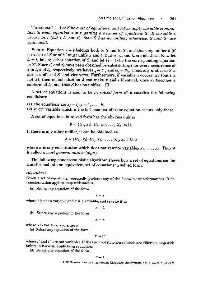
THEOREM 2.2. Let S be a set o f equations, and let us apply variable elimination to some equation x = t, get t ing a new set o f equations S'. I f variable x occurs in t (but t is not x), then S has no unifier; otherwise, S and S ' are equivalent.

PROOF. E q u a t i o n x = t be longs b o t h to S and to S ' , and thus any unif ier v ~ (if it exists) of S or o f S ' m u s t uni fy x and t; t h a t is, xo and to are identical. N o w let tl = t2 be any o the r equa t ion of S, and let t l = t~ be the co r respond ing equa t ion in S'. Since t l and t~ have been ob ta ined by subs t i tu t ing t for eve ry occur rence o f x in tl and t2, respect ively, we have tl~ = t ~ and t2~ = t~ . Thus , any unif ier o f S is also a unif ier o f S ' and vice versa. Fu r t he rmore , if var iable x occurs in t (but t is no t x), t h e n no subs t i tu t ion ~ can m a k e x and t identical, s ince xo b e c o m e s a s u b t e r m of to, and thus S has no unifier. [ ]

A set of equa t ions is said to be in solved form iff it satisfies the fol lowing condit ions:

(1) the equa t ions are xj = ti, j = 1, . . . , k;

(2) every var iable which is the left m e m b e r o f some equa t ion occurs on ly there .

A set of equa t ions in solved fo rm has the obvious unif ier

0 - {(tl, xl), (t2, x2), • . . , (tk, xk)}.

I f t he re is any o the r unifier, it can be ob ta ined as

0 = { ( t , , x~), (t2°, x2) . . . . , ( tk , x k ) } U a

where a is any subs t i tu t ion which does no t rewri te var iables xl . . . . , xk. T h u s t~ is called a most general unifier (mgu ).

T h e following nonde te rmin i s t i c a lgor i thm shows how a set of equa t ions can be t r an s fo rmed into an equ iva len t set o f equa t ions in solved form.

Algorithm 1

Given a set of equations, repeatedly perform any of the following transformations. If no transformation applies, stop with success.

(a) Select any equation of the form

t = x

where t is not a variable and x is a variable, and rewrite it as

(b) Select any equation of the form

where x is variable, and erase it. (c) Select any equation of the form

x = t .

X = X

t ' = t"

where t ' and t" are not variables. If the two root function symbols are different, stop with failure; otherwise, apply term reduction.

(d) Select any equation of the form

x = t



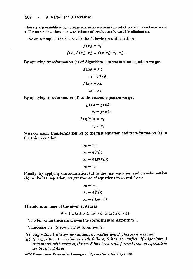
where x is a variable which occurs somewhere else in the set of equations and where t # x. If x occurs in t, then stop with failure; otherwise, apply variable elimination.

As an example, let us consider the following set of equations:

g(x2) = xl;

f (xl , h(xl), x2) = f(g(x3), x4, x3).

By applying t rans format ion (c) of Algor i thm 1 to the second equat ion we get

g(x2) = xl;

xl = g(x3);

h(x~) = x4;

X2 = X 3 .

By applying t rans format ion (d) to the second equat ion we get

g(x2) = g(xs);

xl = g(x3);

h(g(x3)) = x4;

X2 ~- X3.

We now apply t rans format ion (c) to the first equat ion and t rans format ion (a) to the third equation:

X2 ~ X3

xl = g(x3);

Xa = h(g(x3));

X2 ----X3.

Finally, by applying t rans format ion (d) to the first equat ion and t rans format ion (b) to the last equation, we get the set of equat ions in solved form:

X2 ~- X3 ;

xl = g(x3);

x4 = h(g(x3)).

Therefore , an mgu of the given sys tem is

= {(g(x~), x~), (x3, x2), (h(g(x3)), x4)}.

T h e following theo rem proves the correctness of Algor i thm 1.

THEOREM 2.3. Given a set of equations S,

(i) Algorithm 1 always terminates, no matter which choices are made. (ii) I f Algorithm 1 terminates with failure, S has no unifier. I f Algorithm 1

terminates with success, the set S has been transformed into an equivalent set in solved form.



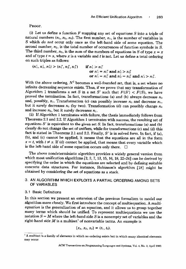
PROOF.

(i) Let us define a function F mapping any set of equations S into a triple of natural numbers (nl, n2, n3). The first number, n~, is the number of variables in S which do not occur only once as the left-hand side of some equation. The second number, n2, is the total number of occurrences of function symbols in S. The third number, n3, is the sum of the numbers of equations in S of type x = x and of type t = x, where x is a variable and t is not. Let us define a total ordering on such triples as follows:

" n~') i fn~ > n~' (n~, n~, n~) > (n~', n 2 ,

o r n~ = n~ a n d n2 > n2 o r n ~ = n " n - ' " ' " 1 a {1 n 2 ---- n2 a n d n 3 > n 3 .

With the above ordering, N 3 becomes a well-founded set, tha t is, a set where no infinite decreasing sequence exists. Thus, if we prove tha t any t ransformat ion of Algorithm 1 t ransforms a set S in a set S' such tha t F(S') < F(S) , we have proved the termination. In fact, t ransformations (a) and (b) always decrease n3 and, possibly, n~. Transformat ion (c) can possibly increase n3 and decrease nl, but it surely decreases n2 (by two). Transformat ion (d) can possibly change n3 and increase n2, but it surely decreases n~.

(ii) If Algorithm 1 terminates with failure, the thesis immediately follows from Theorems 2.1 and 2.2. If Algorithm 1 terminates with success, the resulting set of equations S' is equivalent to the given set S. In fact, t ransformations (a) and (b) clearly do not change the set of unifiers, while for t ransformations (c) and (d) this fact is s tated in Theorems 2.1 and 2.2. Finally, S' is in solved form. In fact, if (a), (b), and (c) cannot be applied, it means tha t the equations are all in the form x = t, with t # x. If (d) cannot be applied, tha t means tha t every v.arialSle which is the left-hand side of some equation occurs only there. []

The above nondeterminist ic algorithm provides a widely general version from which most unification algorithms [2, 3, 7, 13, 15, 16, 18, 22-24] can be derived by specifying the order in which the equations are selected and by defining suitable concrete data structures. For instance, Robinson's algori thm [18] might be obtained by considering the set of equations as a stack.

3. AN ALGORITHM WHICH EXPLOITS A PARTIAL ORDERING AMONG SETS OF VARIABLES

3.1 Basic Definitions

In this section we present an extension of the previous formalism to model our algori thm more closely. We first introduce the concept of multiequation. A multiequation is the generalization of an equation, and it allows us to group together many terms which should be unified. To represent mult iequat ions we use the notat ion S -- M where the left-hand side S is a nonempty set of variables and the r ight-hand side M is a multiset 1 of nonvariable terms. An example is

{xl, x2, x3} = (tl, t2).

A multiset is a family of elements in which no ordering exists but in which many identical elements may occur.



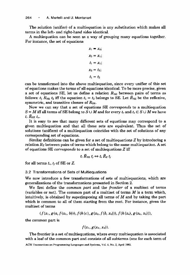
The solution (unifier) of a mult iequat ion is any substi tut ion which makes all te rms in the left- and r ight-hand sides identical.

A mult iequat ion can be seen as a way of grouping many equations together. For instance, the set of equations

Xl ---- X2;

X3 = Xl;

tl = Xl;

X2 ---- t2;

tl = t2

can be t ransformed into the above multiequation, since every unifier of this set of equat ions makes the terms of all equat ions identical. To be more precise, given a set of equations SE, let us define a relat ion RSE between pairs of terms as follows: tl RSE t2 iff the equat ion tl = t2 belongs to SE. Le t / tSE be the reflexive, symmetric , and transitive closure of RSE.

Now we can say tha t a set of equations SE corresponds to a mul t iequat ion S = M iff all terms of SE belong to S U M and for every tr and ts E S U M we have tr RSE t , .

I t is easy to see tha t many different sets of equations may correspond to a given mult iequat ion and tha t all these sets are equivalent. Thus the set of solutions (unifiers) of a mul t iequat ion coincides with the set of solutions of any corresponding set of equations.

Similar definitions can be given for a set of mult iequat ions Z by introducing a relat ion Rz between pairs of terms which belong to the same mult iequation. A set of equations SE corresponds to a set of mult iequat ions Z iff

ti/~SE tj ** ti Rz tj

for all te rms t~, tj of SE or Z.

3.2 Transformat ions of Sets of Mul t iequat ions

We now introduce a few transformations of sets of multiequations, which are generalizations of the t ransformations presented in Sect ion 2.

We first define the common par t and the frontier of a mult iset of terms (variables or not). The common par t of a mult iset of terms M is a t e rm which, intuitively, is obtained by superimposing all te rms of M and by taking the par t which is common to all of t hem start ing from the root. For instance, given the mult iset of terms

( f (x l , g(a, f (xs , b))), f (h (c ) , g(x2, f (b , xs))), f(h(x4), g(x6, x3))),

the common part is

f ( x l , g(x2, x3)).

The frontier is a set of multiequations, where every mul t iequat ion is associated with a leaf of the common part and consists of all subterms (one for each t e rm of



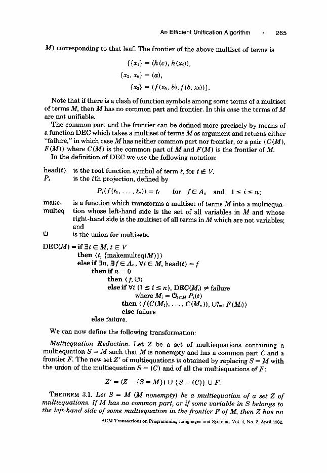
M) corresponding to tha t leaf. The frontier of the above mult ise t of t e rms is

{{x~} = (h(c), h(x4)),

{x2, x6} = (a),

{x3} = (f(xs, b), f(b, xD)).

Note tha t if there is a clash of function symbols among some te rms of a mul t ise t of t e rms M, then M has no com m on pa r t and frontier. In this case the t e rms of M are not unifiable.

T h e commo n par t and the frontier can be defined more precisely by means of a function D E C which takes a mul t ise t of t e rms M as a rgumen t and re turns ei ther "failure," in which case M has nei ther com mon par t nor frontier, or a pair (C(M) , F(M) ) where C(M) is the com m on par t of M and F(M) is the frontier of M.

In the definition of DEC we use the following notation:

head( t ) Pi

makemul teq

is the root function symbol of t e rm t, for t ~ V. is the i th projection, defined by

Pi( f ( t l . . . . , t n ) ) = t i for f ~ A n and l _ < i _ n ;

is a function which t ransforms a mul t ise t of t e rms M into a mul t iequa- t ion whose lef t -hand side is the set of all var iables in M and whose r ight-hand side is the mul t ise t of all t e rms in M which are not variables; and is the union for multisets. t~

D E C ( M ) = f f 3 t ~ M, t E V t h e n (t, {makemul teq(M)} ) e l s e i f 3n, 3 f E A , , Yt E M, head( t ) = f

t h e n i f n ffi 0 t h e n ( f, O) e l se i f Vi (1 __ i _ n), DEC(Mi) ~ failure

where Mi -- OteM Pi(t) t h e n (f(C(M1) . . . . . C(M,)), UTffil F(Mi)) e l se failure

e l se failure.

We can now define the following t ransformat ion:

Multiequation Reduction. Let Z be a set of mul t iequat ions containing a mul t iequat ion S -- M such tha t M is n o n e m p t y and has a common pa r t C and a frontier F. T h e new set Z' of mul t iequat ions is obta ined by replacing S = M with the union of the mul t iequat ion S = (C) and of all the mul t iequat ions of F:

Z ' f f i ( Z - { S f f i M } ) U { S = ( C ) } U F .

THEOREM 3.1. Let S = M (M nonempty) be a multiequation of a set Z of multiequations. I f M has no common part, or if some variable in S belongs to the left-hand side of some multiequation in the frontier F of M, then Z has no



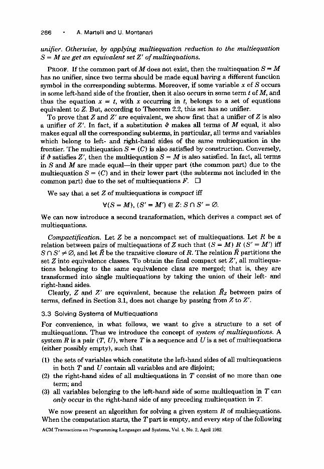
unifier. Otherwise, by applying multiequation reduction to the multiequation S = M we get an equivalent set Z' ofmultiequations.

PROOF. If the common part of M does not exist, then the multiequation S -- M has no unifier, since two terms should be made equal having a different function symbol in the corresponding subterms. Moreover, if some variable x of S occurs in some left-hand side of the frontier, then it also occurs in some term t of M, and thus the equation x = t, with x occurring in t, belongs to a set of equations equivalent to Z. But, according to Theorem 2.2, this set has no unifier.

To prove that Z and Z ' are equivalent, we show first that a unifier of Z is also a unifier of Z'. In fact, if a substitution ~ makes all terms of M equal, it also makes equal all the corresponding subterms, in particular, all terms and variables which belong to left- and right-hand sides of the same multiequation in the frontier. The multiequation S = (C) is also satisfied by construction. Conversely, if ~ satisfies Z', then the multiequation S -- M is also satisfied. In fact, all terms in S and M are made equal--in their upper part (the common part) due to the multiequation S -- (C) and in their lower part (the subterms not included in the common part) due to the set of multiequations F. []

We say that a set Z of multiequations is compact iff

Y(S = M ) , (S' =M '} ~ Z : S A S ' = ~.

We can now introduce a second transformation, which derives a compact set of multiequations.

Compactification. Let Z be a noncompact set of multiequations. Let R be a relation between pairs of multiequations of Z such that iS = M) R iS ' = M') iff S n S' # O, and l e t / t be the transitive closure of R. The relation/~ partitions the set Z into equivalence classes. To obtain the final compact set Z', all multiequations belonging to the same equivalence class are merged; that is, they are transformed into single multiequations by taking the union of their left- and right-hand sides.

Clearly, Z and Z' are equivalent, because the relation /~z between pairs of terms, defined in Section 3.1, does not change by passing from Z to Z'.

3.3 Solving Systems of Multiequations

For convenience, in what follows, we want to give a structure to a set of multiequations. Thus we introduce the concept of system of multiequations. A system R is a pair (T, U), where T is a sequence and U is a set of multiequations {either possibly empty), such that

(1) the sets of variables which constitute the left-hand sides of all multiequations in both T and U contain all variables and are disjoint;

(2) the right-hand sides of all multiequations in T consist of no more than one term; and

(3) all variables belonging to the left-hand side of some multiequation in T can only occur in the right-hand side of any preceding multiequation in T.

We now present an algorithm for solving a given system R of multiequations. When the computation starts, the T part is empty, and every step of the following


An Efficient Unification Algorithm • 267

Algori thm 2 consists of " t ransferr ing" a mul t iequat ion f rom the U part , t ha t is, the unsolved part , to the T part , t ha t is, the triangular or solved par t of R. When the U p a r t of R is empty , the sys tem is essentially solved. In fact, the solution can be obta ined by subst i tut ing the var iables backward. Notice that , by keeping a solved sys tem in this t r iangular form, we can hope to find efficient a lgor i thms for unification even when the mgu has a size which is exponential with respect to the size of the initial system. For instance, the mgu of the set of mul t iequat ions

{{Xl} = ~,

{x~} = ~ ,

{x3} = 0 ,

{x4} = (h(x3, h(x2, x2)), h(h(h (xl, xl), x2), x3))} is

{(h(xl, Xl), x2), (h(h(xl, Xl), h(Xl, Xl)), x3),

(h(h(h(Xl, Xl), h(xl, Xl)), h(h(xl, Xl), h(Xl, Xl))), X4)}.

However , we can give an equivalent solved sys tem with e m p t y U pa r t and whose T pa r t is

({x,} --- (h(x3, x3)),

{x3} = (h(x2, x2)),

{X2) = ( h ( X l , xl)),

{xl} = o ) ,

f rom which the mgu can be obta ined by subst i tut ing backward. Given a sys tem R = (T, U) with an e m p t y T part , an equivalent sys tem with

an e m p t y U pa r t can be computed with the following algori thm.

Algorithm 2 (1) r epea t

(1.1) Select a multiequation S = M of U with M # ~5. (1.2) Compute the common part C and the frontier F ofM. I f M has no common part,

stop with failure (clash). (1.3) If the left-hand sides of the frontier of M contain some variable of S, stop with

failure (cycle). (1.4) Transform U using multiequation reduction on the selected mnltiequation and

compactification. (1.5) Let S = {xl . . . . . Xn). Apply the substitution ~ = {(C, xl) . . . . . (C, x,)} to all

terms in the right-hand side of the multiequations of U. (1.6) Transfer the multiequation S = (C) from U to the end of T. u n t i l the U part of R contains only multiequations, if any, with empty right-hand

sides. (2) Transfer all the mnltiequations of U (all with M = ~D) to the end of T, and stop with

success.

Of course, if we want to use this a lgor i thm for unifying two t e rms tl and t2, we have to construct an initial sys tem with e m p t y T pa r t and with the following U part :

{{x) = (tl, t2), {xl} = 6 , {x2} = O . . . . . {x,} = 6 }



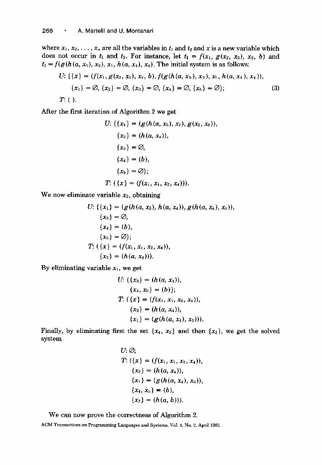
where xl, x2 . . . . , Xn are all the variables in t~ and t2 and x is a new variable which does not occur in ti and t2. For instance, let tl = f(x~, g(x2, xs), x2, b) and t2 = f ( g ( h ( a , xs), x2), x~, h(a, x4), x4). The initial system is as follows:

U: {{x} = ( f ( x l ,g (x2 , x3), x2, b), f ( g ( h ( a , x~), x2), xl, h(a, x4), x4)),

{x~} = 6 , (x2} = 6 , {x3} = ;D, (x4} = 6 , {xs} = 6}; (3)

T : ( ) .

After the first i terat ion of Algori thm 2 we get

U: {(x~} = (g (h(a , x~), x2), g(x2, x3)),

{x2} = (h(a, x4)),

(x~) = 0 ,

(x4} = (b),

(xs} = ~ ) ;

T: ( {x} = (f(xl, xl, x2, x4))).

We now eliminate variable x2, obtaining

U: ({Xl) = (g (h(a , xs), h(a, x4)), g (h (a , x4), x3)),

{x3} = 6 ,

(x4} = (b),

{x5 ) = O};

T: ( (x} = ( f ( x l , Xl, x2, x4)),

{x2} = (h(a, x4))).

By eliminating variable xl, we get

U: {(x3} = (h(a, x4)),

{x,, xs} = (b));

T: ( (x} = ( f(xl , xi, x2, x4)),

(x2} = (h(a, x4)),

(xl} = (g(h(a , x4), x3))).

Finally, by eliminating first the set {x4, xs} and then {x3}, we get the solved system

U: O;

T: ((x} = (f(x~, Xl, X2, X4)),

(X2) = (h(a, x4)),

{Xl) = (g (h(a , x4), xz)),

(x4, xs} = (b),

{x3) = (h(a, b))).

We can now prove the correctness of Algorithm 2.


An Efficient Unification Algorithm • 269

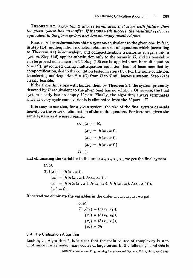
THEOREM 3.2. Algorithm 2 always terminates. I f it stops with failure, then the given system has no unifier. I f it stops with success, the resulting system is equivalent to the given system and has an empty unsolved part.

PROOF. All transformations obtain systems equivalent to the given one. In fact, in step (1.4} multiequation reduction obtains a set of equations which (according to Theorem 3.1) is equivalent, and compactification transforms it again into a system. Step {1.5) applies substitution only to the terms in U, and its feasibility can be proved as in Theorem 2.2. Step (1.6) can be applied since the multiequation S = (C), introduced during multiequation reduction, has not been modified by compactification, due to the condition tested in step (1.3). For the same condition, transferring multiequation S = (C) from U to T still leaves a system. Step (2) is clearly feasible.

If the algorithm stops with failure, then, by Theorem 3.1, the system presently denoted by R (equivalent to the given one) has no solution. Otherwise, the final system clearly has an empty U part. Finally, the algorithm always terminates since at every cycle some variable is eliminated from the U part. []

It is easy to see that, for a given system, the size of the final system depends heavily on the order of elimination of the multiequations. For instance, given the same system as discussed earlier,

U: {{xl) = ~ ,

{x2} = (h(xl, Xl)),

{x3} = (h(x2, x2)),

{x,) = (h(x3, x3))};

T : ( ) ,

and eliminating the variables in the order x2, xz, x4, Xx, we get the final system

U: 0;

T: ({x2) - - (h(xm, Xl ) ) ,

{x3} = (h(h(Xl, xl), h(Xl, xl))),

{x4} = (h(h(h(Xl, Xl), h(xl, xl)), h(h(xl , xl), h(Xl, Xl)))),

{x~ } = 0 ) .

If instead we eliminate the variables in the order x4, x3, x2, xl, we get

U: O;

T: ({x4} = (h(x3, x3)),

(x3} = (h(x2, x2)),

{x2} -- (h(Xl, Xx)),

{x, } = O).

3.4 The Unif icat ion Algor i thm

Looking at Algorithm 2, it is clear that the main source of complexity is step (1.5), since it may make many copies of large terms. In the following--and this is



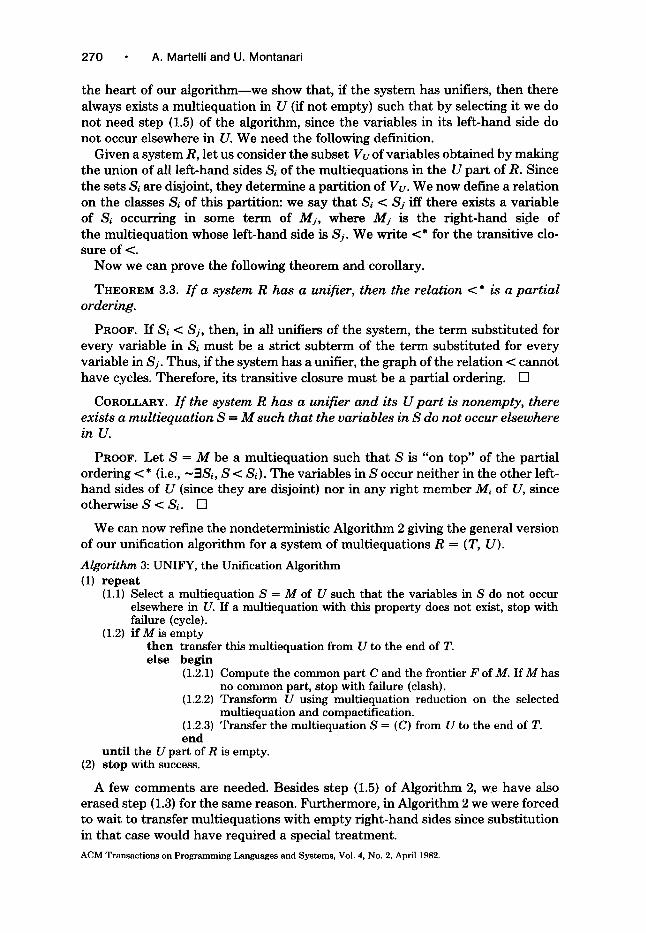
the hear t of our a lgo r i t hm- -we show that , if the sys tem has unifiers, then there always exists a mul t iequat ion in U (if not empty) such t ha t by selecting it we do not need step (1.5) of the algori thm, since the var iables in its lef t -hand side do not occur elsewhere in U. We need the following definition.

Given a sys tem R, let us consider the subset Vu of var iables obta ined by making the union of all lef t -hand sides Si of the mul t iequat ions in the U pa r t of R. Since the sets Si are disjoint, they de te rmine a par t i t ion of Vu. We now define a re la t ion on the classes Si of this parti t ion: we say t ha t Si < Sj iff there exists a var iable of Si occurring in some t e r m of Mj, where Mj is the r ight -hand side of the mul t iequat ion whose lef t -hand side is Sj. We write <* for the t ransi t ive closure of <.

Now we can prove the following theorem and corollary.

THEOREM 3.3. I f a system R has a unifier, then the relation <* is a partial ordering.

PROOF. I f Si < $i, then, in all unifiers of the system, the t e r m subs t i tu ted for every var iable in Si mus t be a str ict s ub t e rm of the t e r m subs t i tu ted for every var iable in Sj. Thus, if the sys tem has a unifier, the graph of the relat ion < cannot have cycles. Therefore , its t ransi t ive closure mus t be a par t ia l ordering. []

COROLLARY. If the system R has a unifier and its U part is nonempty, there exists a multiequation S ffi M such that the variables in S do not occur elsewhere inU.

PROOF. Le t S = M be a mul t iequat ion such t ha t S is "on top" of the par t ia l ordering < * (i.e., ~3Si, S < Si). T h e var iables in S occur nei ther in the o ther left- hand sides of U (since they are disjoint) nor in any r ight m e m b e r Mi of U, since otherwise S < Si. []

We can now refine the nondeterminis t ic Algor i thm 2 giving the general version of our unification a lgor i thm for a sys tem of mul t iequat ions R = (T, U).

Algorithm 3: UNIFY, the Unification Algorithm (1) r epea t

(1.1) Select a multiequation S = M of U such that the variables in S do not occur elsewhere in U. If a multiequation with this property does not exist, stop with failure (cycle).

(1.2) i f M i s empty then transfer this multiequation from U to the end of T. else begin

(1.2.1) Compute the common part C and the frontier F of M. If M has no common part, stop with failure (clash).

(1.2.2) Transform U using multiequation reduction on the selected multiequation and compactification. Transfer the multiequation S = (C) from U to the end of T. (1.2.3)

end until the U part of R

(2) stop with success. is empty.

A few comme n t s are needed. Besides s tep (1.5) of Algor i thm 2, we have also erased step (1.3) for the same reason. Fur thermore , in Algor i thm 2 we were forced to wait to t ransfer mul t iequat ions wi th e m p t y r ight -hand sides since subst i tu t ion in t ha t case would have required a special t r ea tment .



By applying Algorithm UNIFY to the system which was previously solved with Algorithm 2, we see that we must first eliminate variable x, then variable x,, then variables x2 and x3 together, and, finally, variables x4 and x5 together, getting the following final system:

U : ~

T: ( { x } = ( f ( x l , x l , x2, x , ) ) ,

{Xl} = (g(x2, x3)),

{x2, x3} = (h(a, x4)), {x,, xs} = (b)).

Note that the solution obtained using Algorithm UNIFY is more concise than the solution previously obtained using Algorithm 2, for two reasons. First, variables x2 and x3 have been recognized as equivalent; second, the right member of x~ is more factorized. This improvement is not casual but is intrinsic in the ordering behavior of Algorithm UNIFY.

To summarize, Algorithm UNIFY is based mainly on the two ideas of keeping the solution in a factorized form and of selecting at each step a multiequation in such a way that no substitution ever has to be applied. Because of these two facts, the size of the final system cannot be larger than that of the initial one. Furthermore, the operation of selecting a multiequation fails if there are cycles among variables, and thus the so-called occur-check is built into the algorithm, instead of being performed at the last step as in other algorithms [2, 7].

4. EFFICIENT MULTIEQUATION SELECTION

In this section we show how to implement efficiently the operation of selecting a multiequation "on top" of the partial ordering in step (1.1) of Algorithm 3.

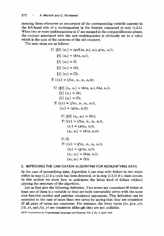
The idea is to associate with every multiequation a counter which contains the number of other occurrences in U of the variables in its left-hand side. This counter is initialized by scanning the whole U part at the beginning. Of course, a multiequation whose counter is set to zero is on top of the partial ordering.

For instance, let us again consider system (3):

U: {[0] {x} = (f(xl,g(x2, x3), x2, b), f(g(h(a, x~), xe), xl,

h(a, x4), x4)),

[2] {xl} = 6,

[3] {x2} = 6,

[1] (x3} = 6 ,

[2] {x4} = 6,

[1] {xa} -- 6};

T:().

Here square brackets enclose the counters associated with each multiequation. Since only the first multiequation has its counter set to zero, it is selected to be transferred. Counters of the other multiequations are easily updated by decre-



ment ing t hem whenever an occurrence of the corresponding variable appears in the lef t -hand side of a mul t iequat ion in the frontier computed in step {1.2.1). When two or more mul t iequat ions in U are merged in the compact i f icat ion phase, the counter associated with the new mul t iequat ion is obviously set to a value which is the sum of the contents of the old counters.

T h e next s teps are as follows:

U: {[0] (Xl} = (g(h(a, x~), x2), g(x2, x3)),

[2] {x2} = (h(a, x4)),

[1] (x~) = o,

[1] {x , } = (b),

[1] {x~} = ~};

T: ( (x} = (f(xl, x~, x2, x4))).

U: {[0] {x2, x3} = (h(a, x4), h(a, x~)),

[1] {x4} = (b),

[1] {x~} = o} ;

T: ({x} = (f(x,, x,, x2, x,)) ,

{x,} = (g(x2, x3))).

U: {[0] {x4, xs} = (b)};

T: ({x} = (f(x,, xl, x2, x4)), { x , } = (g(x2, x3)), {x2, x3} = (h(a, x4))).

U: ~;

T: ({x} = (f(xl, xl, x2, x4)),

{xl} = (g(x2, x3)),

{x2, x3} = (h(a, x4)),

{x4, x~} = (b)).

5. IMPROVING THE UNIFICATION ALGORITHM FOR NONUNIFYING DATA

In the case of nonunifying data, Algor i thm 3 can stop with failure in two ways: e i ther in s tep (1.1) if a cycle has been detected, or in s tep (1.2.1) if a clash occurs. In this section we show how to ant ic ipate the la t ter kind of failure wi thout al tering the s t ruc ture of the algori thm.

Let us first give the following definition. Two t e rms are consistent iff e i ther a t least one of t h e m is a var iable or they are bo th nonvar iable t e rms with the same root funct ion symbol and pairwise consis tent arguments . Th is definit ion can be extended to the case of more than two t e rms by saying t ha t they are consis tent iff all pairs of t e rms are consistent. For instance, the three t e rms f(x, g(a, y)), f(b, x), and f(x, y) are consis tent a l though they are not unifiable.



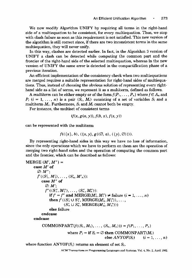
We now modify Algorithm UNIFY by requiring all te rms in the r ight-hand side of a mult iequat ion to be consistent, for every multiequation. Thus, we stop with clash failure as soon as this requi rement is not Satisfied. This new version of the algori thm is still correct since, if there are two inconsistent terms in the same multiequation, they will never unify.

In this way, clashes are detected earlier. In fact, in the Algorithm 3 version of UNIFY a clash can be detected while computing the common par t and the frontier of the r ight-hand side of the selected multiequation, whereas in the new version of UNIFY the same error is detected in the compactification phase of a previous iteration.

An efficient implementat ion of the consistency check when two mult iequat ions are merged requires a suitable representat ion for r ight-hand sides of multiequations. Thus, instead of choosing the obvious solution of representing every right- hand side as a list of terms, we represent it as a mult i term, defined as follows.

A mult i term can be ei ther empty or of the form f(P1 . . . . . Pn) where f E A, and Pi (i = 1 . . . . . n) is a pair (Si, Mi) consisting of a set of variables Si and a mul t i term ]Vii. Furthermore , Si and Mi cannot bo th be empty.

For instance, the multiset of consistent terms

(f(x, g(a, y)), f(b, x), f(x, y))

can be represented with the mul t i term

f ( ( (x} , b), ( { x , y } , g ( ( O , a) , ( (y ) , ~ ) ) ) ) .

By representing r ight-hand sides in this way we have no loss of information, since the only operations which we have to perform on them are the operat ion of merging two r ight-hand sides and the operat ion of computing the common part and the frontier, which can be described as follows:

M E R G E (M', M " ) = c a s e M ' o f

O: M " ; f ' ( ( S i M~), , t S ' M ' ~"

c a s e M" o f O: M'; f " ( (S~ ' ,M~' ) . . . . . (Sn", M~")):

i f f ' -- f " a n d MERGE(M~, M[') # failure (i -- 1 . . . . . n) t h e n f ' ( ( S i O S~', MERGE(MI , M; ' ) ) . . . . .

( S ~ ~J S t'n, MERGE(M~', M,,))"~ e l se failure

e n d c a s e e n d c a s e

COMMONPART(f ( (S1 , M1) . . . . . (S , , Mn))) = f(P1, - - . , Pn)

where Pi = i f Si = ~ t h e n COMMONPART(Mi) e l se A N Y O F ( S D (i = 1 . . . . , n)

where function ANYOF(S~) returns an e lement of set Si.



F i g u r e 1

UPart = r e c o r d

MultEqNumber: Integer;, ZeroCounterMultEq, Equations: Lis tOfMultEq

end; System = TPSystem; PSystem = r e c o r d

T: ListOfMultEq; U: UPart

end; Mult iTerm = ~PMultiTerm; PMul t iTerm = r e c o r d

Fsymb: FunName; Args: L is tOfTempMul tEq

end; Mult iEquat ion = ~PMultiEquation; PMult iEquat ion = record

Counter, VarNumber: Integer; S: ListOfVariables; M: Mul t i Term

e n d ;

TempMultEq = ~PTempMultEq; PTempMul tEq = r e c o r d

S: QueueOfVariables; M: MultiTerrn

e n d ;

Variable = TPVariable; P Variable = r e c o r d

Name: VarName; M: Mult iEquat ion

e n d ;

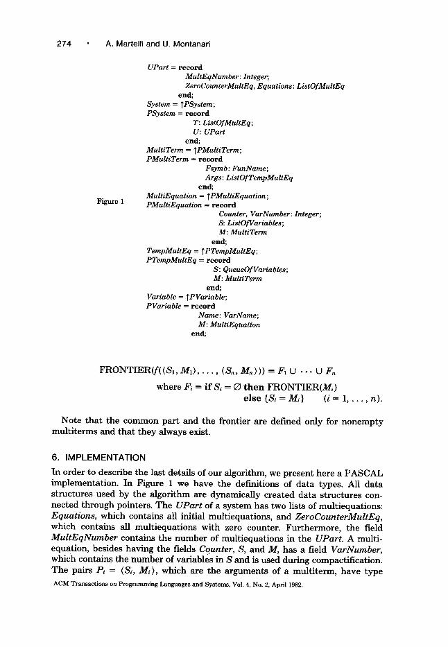
FRONTIER(f((S, , M1) . . . . . ( S n , M n ) )) = F1 [..J . . . (.J Fn

where Fi = if Si = O t h e n FRONTIER(M/) else {Si = M i } ( i = 1, . . . , n ) .

Note that the common part and the frontier are defined only for nonempty multiterms and that they always exist.

6. IMPLEMENTATION

In order to describe the last details of our algorithm, we present here a PASCAL implementation. In Figure 1 we have the definitions of data types. All data structures used by the algorithm are dynamically created data structures con- nected through pointers. The UPart of a system has two lists of multiequations: Equations, which contains all initial multiequations, and ZeroCounterMultEq, which contains all multiequations with zero counter. Furthermore, the field MultEqNumber contains the number of multiequations in the UPart. A multiequation, besides having the fields Counter, S, and M, has a field VarNumber, which contains the number of variables in S and is used during compactification. The pairs Pi = (S i, Mi), which are the arguments of a multiterm, have type



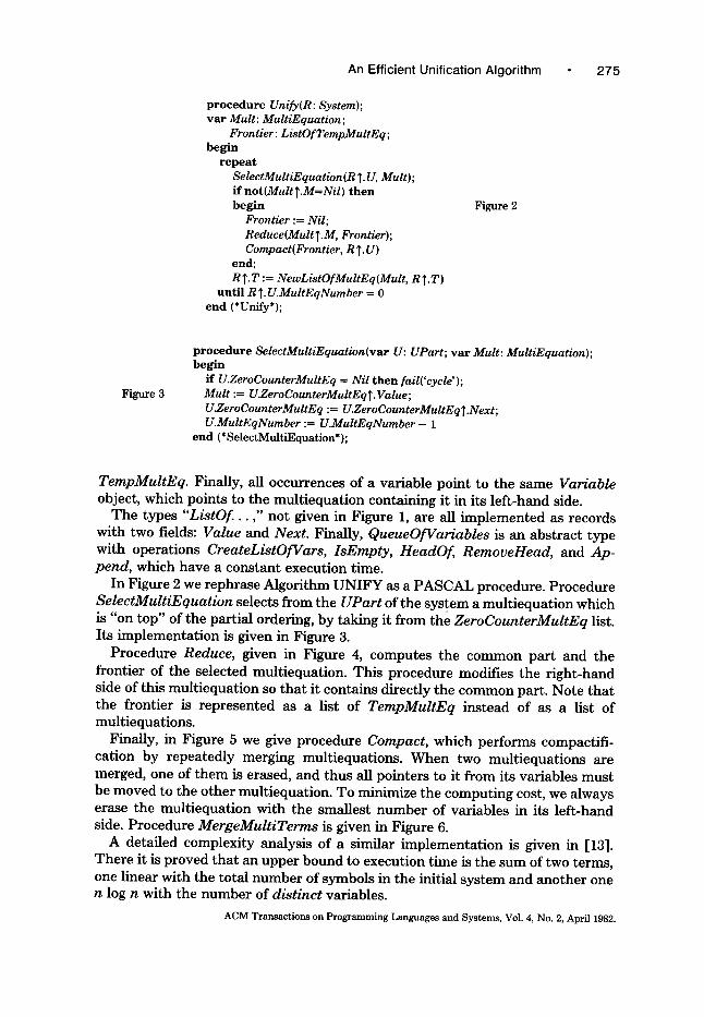
procedure Unify(R: System); var Mult: MultiEquation ;

Frontier: ListOf TempMultEq ; b e g i n

repeat SelectMultiEquation(R ~. U, Mult); i f not(Mult~.M=Nil) then b e g i n

Frontier := Nil; Reduce(Multi.M, Frontier); Compact(Frontier, R ~. U)

end; R ~.T := NewListOfMultEq(Mult, R ~.T)

unti l R ~. U.MultEqNumber = 0 end (*Unify*);

Figure 2

Figure 3

procedure SelectMultiEquation(var U: UPart; v a r Mult: MultiEquation); b e g i n

i f U.ZeroCounterMultEq = Nil t h e n fail('cycle'); Mult := U~eroCounterMultEq~. Value; U~eroCounterMultEq := U.ZeroCounterMultEqT.Next; U.MultEqNumber := U.MultEqNumber - 1

end ( * SelectMult iEquation *);

TempMultEq. Finally, all occurrences of a variable point to the same Variable object, which points to the multiequation containing it in its left-hand side.

The types "ListOf... ," not given in Figure 1, are all implemented as records with two fields: Value and Next. Finally, QueueOfVariables is an abstract type with operations CreateListOfVars, IsEmpty, HeadOf, RemoveHead, and Ap- pend, which have a constant execution time.

In Figure 2 we rephrase Algorithm UNIFY as a PASCAL procedure. Procedure SelectMultiEquation selects from the UPart of the system a multiequation which is "on top" of the partial ordering, by taking it from the ZeroCounterMultEq list. Its implementation is given in Figure 3.

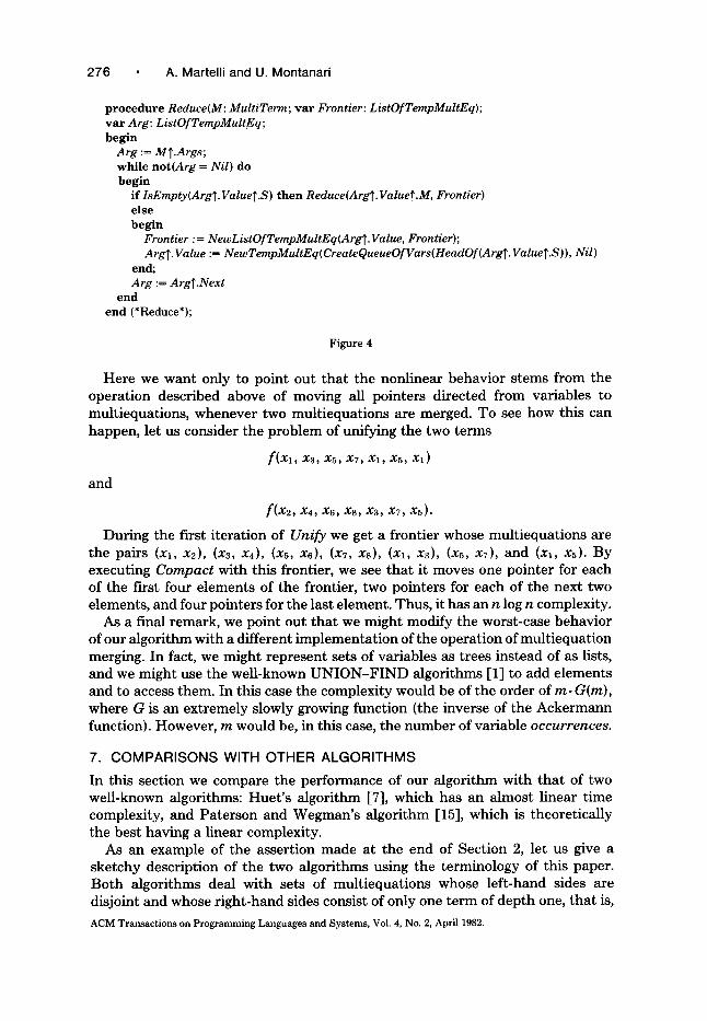
Procedure Reduce, given in Figure 4, computes the common part and the frontier of the selected multiequation. This procedure modifies the right-hand side of this multiequation so that it contains directly the common part. Note that the frontier is represented as a list of TempMultEq instead of as a l is t of multiequations.

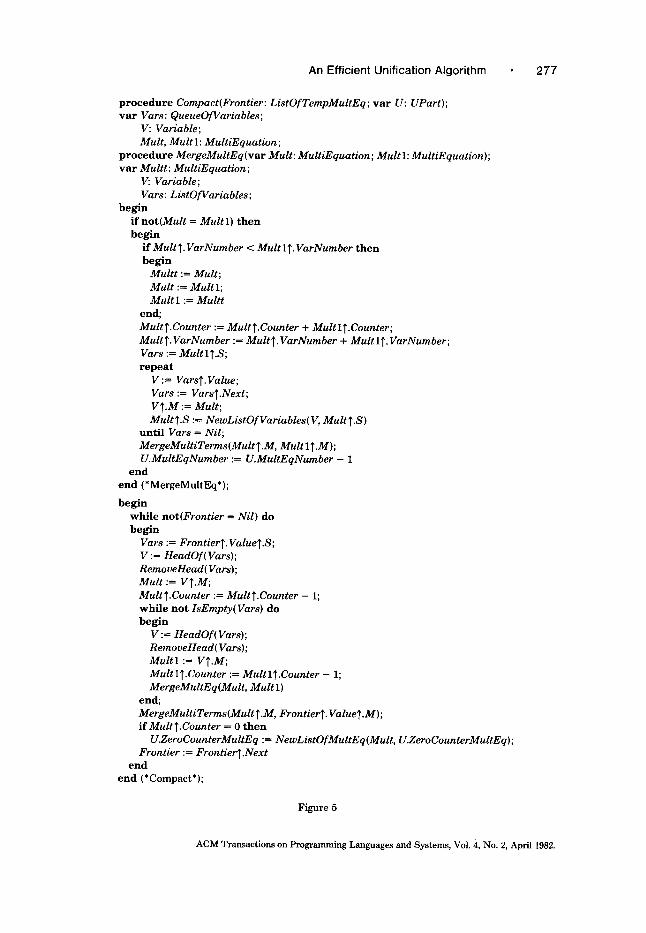
Finally, in Figure 5 we give procedure Compact, which performs compactification by repeatedly merging multiequations. When two multiequations are merged, one of them is erased, and thus all pointers to it from its variables must be moved to the other multiequation. To minimize the computing cost, we always erase the multiequation with the smallest number of variables in its left-hand side. Procedure MergeMultiTerms is given in Figure 6.

A detailed complexity analysis of a similar implementation is given in [13]. There it is proved that an upper bound to execution time is the sum of two terms, one linear with the total number of symbols in the initial system and another one n log n with the number of distinct variables.



procedure Reduce(M: MultiTerm; var Frontier: ListOfTernpMultEq); var Arg" ListOfTempMultEq; b e g i n

Arg := MT.Args; w h i l e not(Arg = Nil) do begin

i f IsEmpty(Arg T. Value T.S) then Reduce(ArgO. Value T.M, Frontier) else b e g i n

Frontier := NewListOfTempMultEq(Arg T. Value, Frontier); ArgT. Value := NewTempMultEq( CreateQueueOfVars(HeadOf(Arg~. ValueT.S) ) , Nil)

end; Arg := ArgT.Next

end end (*Reduce*);

Figure 4

Here we want only to point out that the nonlinear behavior stems from the operation described above of moving all pointers directed from variables to multiequations, whenever two multiequations are merged. To see how this can happen, let us consider the problem of unifying the two terms

f ( x l , x3, xs, xT, xl , xs, x l )

and

f(x2, x4, x6, x8, x3, x7, x5).

During the first iteration of Unify we get a frontier whose multiequations are the pairs (xl, x2), (x3, x4), (x~, x6), (xT, xs), (xl, x3), (xs, xT), and (xl, xs). By executing Compact with this frontier, we see that it moves one pointer for each of the first four elements of the frontier, two pointers for each of the next two elements, and four pointers for the last element. Thus, it has an n log n complexity.

As a final remark, we point out that we might modify the worst-case behavior of our algorithm with a different implementation of the operation of multiequation merging. In fact, we might represent sets of variables as trees instead of as lists, and we might use the well-known UNION-FIND algorithms [1] to add elements and to access them. In this case the complexity would be of the order of m. G(m), where G is an extremely slowly growing function (the inverse of the Ackermann function). However, m would be, in this case, the number of variable occurrences.

7. COMPARISONS WITH OTHER ALGORITHMS

In this section we compare the performance of our algorithm with that of two well-known algorithms: Huet 's algorithm [7], which has an almost linear time complexity, and Paterson and Wegman's algorithm [15], which is theoretically the best having a linear complexity.

As an example of the assertion made at the end of Section 2, let us give a sketchy description of the two algorithms using the terminology of this paper. Both algorithms deal with sets of multiequations whose left-hand sides are disjoint and whose right-hand sides consist of only one term of depth one, that is,



p r o c e d u r e Compact(Frontier: Lis tOfTempMultEq; v a r U: UPart); v a r Vars: QueueOfVariables;

V: Variable; Mult, Mul t 1: Mult iEquation ;

p r o c e d u r e MergeMultEq(var Mult: Mult iEquation ; Mul t l: Mult iEquation ); v a t Multt: MultiEquation;

V: Variable; Vars : L istOfVariab les ;

b e g i n i f not (Mul t = Mul t 1) t h e n b e g i n

i f Mult T. VarNumber < Mul t 1T. VarNumber t h e n b e g i n

Mult t := Mult; Mul t := Mul t l ; Mul t 1 := Mult t

end;

MultT.Counter := MultT.Counter + Multl~.Counter; Mul t T. VarNumber := Mul t ~. VarNumber + Mul t 1 T. VarNumber; Vars := Mult l T.S; r e p e a t

V := Vars'~.Value; Vars := VarsT.Next; V ~.M := Mult; Mul t T.S := NewListOfVariables( V, Mul t T.S)

un t i l Vars = Nil; MergeMultiTerms(MultT.M, Mul t l T.M); U.MultEqNumber := U . M u l t E q N u m b e r - 1

end end (*MergeMultEq*);

b e g i n whi le not(Frontier = Nil) do b e g i n

Vars := Frontier T. ValueT.S; V := HeadOf(Vars); RemoveHead( Vars); Mul t := VT.M; MultT.Counter := MultT.Counter - 1; wh i l e n o t IsEmpty(Vars) do b e g i n

V := HeadOf(Vars); RemoveHead( Vars); M u l t l :-- VT.M; Mul t l T.Counter := Mult l ~.Counter - 1; MergeMultEq(Mult, Mul t 1)

end; MergeMulti Terms(Mult T.M, Frontier T. Value~.M ) ; i fMultT.Counter = 0 t h e n

U.ZeroCounterMultEq := NewListOfMultEq(Mult , U.ZeroCounterMultEq); Frontier := FrontierT.Next

end end (*Compact*);

Figure 5

ACM Transactions on Programming Languages and Systems, Vol. ~1, No. 2, April 1982.


Figure 6

p r o c e d u r e MergeMultiTerms(var M: MultiTerm ; MI: MultiTerm); v a r Arg, Argl: ListOfTempMultEq; begin

i f M = Nil t h e n M := M1 e l s e i f no t (M1 = Nil) t h e n begin

if not (M "f .Fsymb = M l ~.Fsymb) then fail(' clash' ) else begin

Arg := M~.Args; Argl := MIT.Args; while not(Arg = Nil) do begin

Append(Arg~. Value~.S, Argl ~. Value~.S); MergeMultiTerms(Arg~. Value~.M, Argl ~. Value~.M ); Arg := ArgT.Next; Argl := ArglT.Next

e n d e n d

e n d e n d (*MergeMultiTerms*);

o f t h e f o r m f ( x , , . . . , x , ) w h e r e x, . . . . . Xn are va r i ab l e s . F o r i n s t ance ,

{x , } = f(x~, x3, x , ) ;

F u r t h e r m o r e , we h a v e a s e t S va r i ab le s ; for i n s t ance ,

{x2} --- a ;

(xa} = g(x2);

(x4} = a ;

(x5} ffi f(x6, xT, xs);

{x6} = a ;

{x7} = g(xa) ;

(4)

{xs} = O.

of e q u a t i o n s w h o s e lef t - a n d r i g h t - h a n d s ides a r e

S: {x, = xs} .

A s t e p o f b o t h a l g o r i t h m s cons i s t s o f c h o o s i n g a n e q u a t i o n f r o m S, m e r g i n g t h e two c o r r e s p o n d i n g m u l t i e q u a t i o n s , a n d a d d i n g to S t h e n e w e q u a t i o n s o b t a i n e d as t h e o u t c o m e o f t h e merg ing . F o r i n s t ance , a f t e r t h e f i r s t s t e p we h a v e

{x, , xs} = f(x2, x~, x4);

{X2} = a ;

{x3) = g(x2) ;

{x4} = a ;

{x~} = a ;

{xv} = g(xa) ;

{x8 } = O;

S: {x2 = x6, x3 ffi x7, x4 = xs ) .


(5)


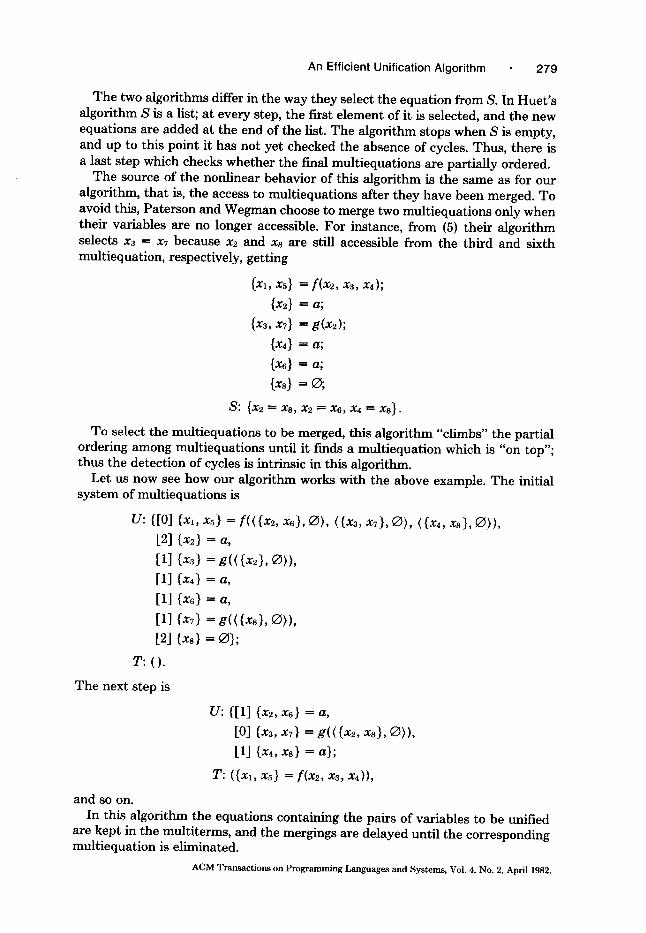
The two algorithms differ in the way they select the equation from S. In Huet 's algorithm S is a list; at every step, the first element of it is selected, and the new equations are added at the end of the list. The algorithm stops when S is empty, and up to this point it has not yet checked the absence of cycles. Thus, there is a last step which checks whether the final multiequations are partially ordered.

The source of the nonlinear behavior of this algorithm is the same as for our algorithm, tha t is, the access to multiequations after they have been merged. To avoid this, Paterson and Wegman choose to merge two multiequations only when their variables are no longer accessible. For instance, from (5) their algorithm selects x3 = x7 because x2 and xs are still accessible from the third and sixth multiequation, respectively, getting

{xl, xs} = f(x2, x3, x,);

{x2} = a;

{x3, xT} = g(x2);

{x4} = a;

{x6} =- a;

{xs} = O;

S: {x2 = xs, x2 = x6, x4 = xs}.

To select the multiequations to be merged, this algorithm "climbs" the partial ordering among multiequations until it finds a multiequation which is "on top"; thus the detection of cycles is intrinsic in this algorithm.

Let us now see how our algorithm works with the above example. The initial system of multiequations is

U : {[0] {Xl, X5} = f(( {x2, x6}, O), ({x3, xT}, gD), ({x4, xs}, ~) ) ,

[2] {x2} -= a,

[1] {x3} = g(({x2), O)),

[1] (x4} = a,

[1] {x6} = a,

[1] {xT} = g({{xs}, O)),

[2] {xs ) = ~};

T: ().

The next step is

U: {[1] {x2, x6} = a,

[0] {x3, xT) = g(({x2, xs}, ~) ) ,

[1] {x4, xs} = a};

T: ((x~, xs} = f(x2, x~, x4)),

and so on. In this algorithm the equations containing the pairs of variables to be unified

are kept in the multiterms, and the mergings are delayed until the corresponding multiequation is eliminated.



An important difference between our algorithm and the others is that our algorithm may use terms of any depth. This fact entails a gain in efficiency, because it is certainly simpler to compute the common part and the frontier of deep terms than to merge multiequations step by step. Note, however, that this feature might also be added to the other algorithms. For instance, by adding the capability of dealing with deep terms to Paterson and Wegman's algorithm, we essentially obtain a linear algorithm which was independently discovered by the authors [13].

In order to compare the essential features of the three algorithms, we notice that they can stop either with success or with failure for the detection of a cycle or with failure for the detection of a clash. Let Pm, Pc, and Pt be the probabilities of stopping with one of these three events, respectively. We consider three extreme cases:

(1) Pm >> Pc, Pt {very high probability of stopping with success). Paterson and Wegman's algorithm is asymptotically the best, because it has a linear complexity whereas the other two algorithms have a comparable nonlinear complexity.

However, in a typical application, such as, for example, a theorem prover, the unification algorithm is not used for unifying very large terms, but instead it is used a great number of times for unifying rather small terms each time. In this case we cannot exploit the asymptotically growing difference between linear and nonlinear algorithms, and the computing times of the three algorithms will be comparable, depending on the efficiency of the implementation.

An experimental comparison of these algorithms, together with others, was carried out by Trum and Winterstein [21]. The algorithms were implemented in the same language, PASCAL, with similar data structures, and tried on five different classes of unifying test data. Our algorithm had the lowest running time for all test data. In fact, our algorithm is more efficient than Huet's because it does not need a final acyclicity test, and it is more efficient than Paterson and Wegman's because it needs simpler data structures.

(2) Pc >> Pt >> Pm (very high probability of detecting a cycle). Paterson and Wegman's algorithm is the best because it starts merging two multiequations only when it is sure that there are no cycles above them. Our algorithm is also good because cycle detection is embedded in it. In contrast, Huet's algorithm must complete all mergings before being able to detect a cycle, and thus it has a very poor performance.

(3) Pt >> Pc >> Pm (very high probability of detecting a clash). Huet's algorithm is the best because, if it stops with a clash, it has not paid any overhead for cycle detection. Our algorithm is better than Paterson and Wegman's because clashes are detected during multiequation merging and because our algorithm may merge some multiequations earlier, like {x2, x6} and {x4, Xs} in the above example. On the other hand, mergings which are delayed by our algorithm, by putting them in multiterms, cannot be done earlier by the other algorithm because they refer to multiequations which are still accessible. The difference in the performance of the two algorithms may become quite large if terms of any depth are allowed. ACM Transactions on Programming Languages and Systems, Vol. 4, No. 2, April 1982.


8. CONCLUSION

A new unification algorithm has been presented. Its performance has been compared with that of other well-known algorithms in three extreme cases: high probability of stopping with success, high probability of detecting a cycle, and high probability of detecting a clash. Our algorithm was shown to have a good performance in all the cases, and thus presumably in all the intermediate cases, whereas the other algorithms had a poor performance in some cases.

Most applications of the unification algorithm, such as, for instance, a resolution theorem prover or the interpreter of an equation language, require repeated use of the unification algorithm. The algorithm described in this paper can be very efficient even in this case, as the authors have shown in [12]. There they have proposed to merge this unification algorithm with Boyer and Moore's technique for storing shared structures in resolution-based theorem provers [3] and have shown that, by using the unification algorithm of this paper instead of the standard one, an exponential saving of computing time can be achieved. Further- more, the time spent for initializations, which might be heavy for a single execution of the unification algorithm, is there reduced through a close integration of the unification algorithm into the whole theorem prover.

REFERENCES

1. AHO, A.V., HOPCROFT, J.E., AND ULLMAN, J.D. The Design and Analysis of Computer Algo- rithms. Addison-Wesley, Reading, Mass., 1974.

2. BAXTER, L.D. A practically linear unification algorithm. Res. Rep. CS-76-13, Dep. of Applied Analysis and Computer Science, Univ. of Waterloo, Waterloo, Ontario, Canada.

3. BOYER, R.S., AND MOORE, J.S. The sharing of structure in theorem-proving programs. In Machine Intelligence, vol. 7, B. Meltzer and D. Michie (Eds.). Edinburgh Univ. Press, Edinburgh, Scotland, 1972, pp. 101-116.

4. BURSTALL, R.M., AND DARLINGTON, J. A transformation system for developing recursive programs. J. ACM 24, 1 (Jan. 1977), 44-67.

5. CHANG, C.L., AND LEE, R.C. Symbolic Logic and Mechanical Theorem Proving. Academic Press, New York, 1973.

6. HEWITT, C. Description and Theoretical Analysis (Using Schemata) of PLANNER: A Language for Proving Theorems and Manipulating Models in a Robot. Ph.D. dissertation, Dep. of Mathe- matics, Massachusetts Institute of Technology, Cambridge, Mass., 1972.

7. HUET, G. R6solution d'6quations dans les langages d'ordre 1, 2 . . . . . 0:. Th~se d'6tat, Sp6cialit6 Math~matiques, Universit~ Paris VII, 1976.

8. HUET, G.P. A unification algorithm for typed ?,-calculus. Theor. Comput. Sci. 1, 1 (June 1975), 27-57.

9. KNUTH, D.E., AND BENDIX, P.B. Simple word problems in universal algebras. In Computational Problems in Abstract Algebra, J. Leech (Ed.). Pergamon Press, Eimsford, N.Y., 1970, pp. 263-297.

10. KOWALSKI, R. Predicate logic as a programming language. In Information Processing 74, Elsevier North-Holland, New York, 1974, pp. 569-574.

11. LEVI, G., AND SIROVICH, F. Proving program properties, symbolic evaluation and logical proce- dural semantics. In Lecture Notes in Computer Science, vol. 32: Mathematical Foundations of Computer Science 1975. Springer-Verlag, New York, 1975, pp. 294-301.

12. MARTELLI, A., AND MONTANARI, U. Theorem proving with structure sharing and efficient unification. Internal Rep. S-77-7, Ist. di Scienze della Informazione, University of Pisa, Pisa, Italy; also in Proceedings of the 5th International Joint Conference on Artificial Intelligence, Boston, 1977, p. 543.

13. MARTELLI, A., AND MONTANARI, V. Unification in linear time and space: A structured presen-


282 • A Martelli and U. Montanari

tation. Internal Rep. B76-16, Ist. di Elaborazione delle Informazione, Consiglio Nazionale delle Ricerche, Pisa, Italy, July 1976.

14. MILNER, R. A theory of type polymorphism in programming. J. Comput. Syst. Sci. 17, 3 (Dec. 1978), 348-375.

15. PATERSON, M.S., AND WEGMAN, M.N. Linear unification. J. Comput. Syst. Sci. 16, 2 (April 1978), 158-167.

16. ROBINSON, J.A. Fast unification. In Theorem Proving Workshop, Oberwolfach, W. Germany, Jan. 1976.

17. ROBINSON, J.A. Computational logic: The unification computation. In Machine Intelligence, vol. 6, B. Meltzer and D. Michie (Eds.). Edinburgh Univ. Press, Edinburgh, Scotland, 1971, pp. 63-72.

18. ROBINSON, J.A. A machine-oriented logicbased on the resolution principle. J. ACM 12, 1 (Jan. 1965), 23-41.

19. SHORTLIFFE, E.H. Computer-Based Medical Consultation: MYCIN. Elsevier North-Holland, New York, 1976.

20. STICKEL, M.E. A complete unification algorithm for associative-commutative functions. In Proceedings of the 4th International Joint Conference on Artificial Intelligence, Tbilisi, U.S.S.R., 1975, pp. 71-76.

21. TRUM, P., AND WINTERSTEIN, G. Description, implementation, and practical comparison of unification algorithms. Internal Rep. 6/78, Fachbereich Informatik, Univ. of Kaiserlautern, W. Germany.

22. VENTURINI ZILLI, M. Complexity of the unification algorithm for first-order expressions. Calcolo 12, 4 (Oct.-Dec. 1975), 361-372.

23. VON HENKE, F.W., AND LUCKHAM, D.C. Automatic program verificationIII: A methodology for verifying programs. Stanford Artificial Intelligence Laboratory Memo AIM-256, Stanford Univ., Stanford, Calif., Dec. 1974.

24. WALDINGER, R.J., AND LEVITT, K.N. Reasoning about programs. Artif. Intell. 5, 3 (Fall 1974), 235-316.

25. WARREN, D.H.D., PEREIRA, L.M., AND PEREIRA, F. PROLOG--The language and its implementation compared with LISP. In Proceedings of Symposium on Artificial Intelligence and Programming Languages, Univ. of Rochester, Rochester, N.Y., Aug. 15-17, 1977. Appeared as joint issue: SIGPLAN Notices (ACM) 12, 8 (Aug. 1977), and SIGART Newsl. 64 (Aug. 1977), 109-115.

Received September 1979; revised July 1980 and September 1981; accepted October 1981


Documents

An Efficient Unification Algorithm - nsl.com · An Efficient Unification Algorithm 259 Resolution, however, is not the only application of the unification algorithm. In fact, its