General rights Copyright and moral rights for the publications made accessible in the public portal are retained by the authors and/or other copyright owners and it is a condition of accessing publications that users recognise and abide by the legal requirements associated with these rights.

Users may download and print one copy of any publication from the public portal for the purpose of private study or research.

You may not further distribute the material or use it for any profit-making activity or commercial gain

You may freely distribute the URL identifying the publication in the public portal If you believe that this document breaches copyright please contact us providing details, and we will remove access to the work immediately and investigate your claim.

Downloaded from orbit.dtu.dk on: Dec 02, 2021

Approximate methods for 3D overall calculations on light-water reactors

Larsen, Hans Hvidtfeldt

Publication date:1972

Document VersionPublisher's PDF, also known as Version of record

Link back to DTU Orbit

Citation (APA):Larsen, H. H. (1972). Approximate methods for 3D overall calculations on light-water reactors. Risø NationalLaboratory. Denmark. Forskningscenter Risoe. Risoe-R No. 270

o Risø mmn m. 270 <s o Z -*̂ t-i

<g Danish Atomic Energy Commission

2 Research Establishment Risø

Approximate Methods

for 3D Overall Calculations

on Light Water Reactors

by Hans Larsen

July 1972

JWM *rtr**eri: IwL OJribrap. 17, Mvfwte, DK-1J07 Copwhif« K, D«uurk ArdUbt* M txtkmpfnm: Utonij, Dttfcfc Atoafc lafffjr C t w W n , Riw, DK-4000 KMUM«, D n t u t

U.D.C.

July, 1972 Rise Report No. 270

Approximate Methods for 3D Overall Calculations on Light Water Reactors

by

Hans Larsen

Danish Atomic Energy Commission Research Establishment Ris« Reactor Physics Department

Abstract

The applicability of the different approximate methods used for the solution of the three-dimensional diffusion equation is discussed. The flux synthesis program SYNTRGN has been coupled with hydraulics and quasi-stationary burn-up treatment to be used for boiling water reactor calcu­lations. Test calculations are presented.

This report was written in partial fulfilment of the requirements for obtaining the Ph. D. (lie. techn.) degree.

ISBN 17 W 01« *

- 1 -

CONTENTS

Page

1. Introduction 3

2. Solution of the Three-Dimensional Diffusion Equation 4

2.1. Difference Equation Technique 6

2.2. Coarse-Mesh Methods 11 2 .2 .1 . Nodal Theory 11

2 .2 .1 .1 . The Flare Model 12 2 .2 .1 .2 . The Trilux Model 13 2.2. 1.3. Determination of the g-Factors,

Correlations 14 2.2 .2 . Other Coarse-Mesh Methods 14

2.3. Flux Synthesis Methods 15 2 .3 .1 . Ordinary Flux Synthesis 15 2.3.2. Variational Flux Synthesis 17

2.4. Discussion of the Different Approximative Methods 19

3. The Three-Dtøensional Flux Synthesis Program SYNTRON . . . . 21

3 .1 . The Principles for the Construction and the Solution of the Flux Synthesis Equation 21

3.2. The Eigenvalue, Different Criticality Options 24 3.3. The Selection of the Trial Functions 25 3.4. The Calculation of the Trial Functions 25 3.5. Static Test Calculations 26

4. The SYNTRON/VOID Burn-up Program 28

4 .1 . Cross Section Interpolation 28 4.2. The Burn-up Treatment 28 4.3. The Xenon Treatment 29 4.4. The Void and Temperature Calculations 29 4.5. The Doppler Effect 30 4.6. The Control Rod Treatment 30 4.7. The Time Step 31 4.8. The Coupled Program . * 31 4 .9 . Optimal Calculation Strategy 33 4.10. Calculations performed with the SYNTRON/VOID

Program *. 37

. 2 .

Page

5. Summary 39

Appendix A. Teat Krampile for Comparison Between DC4 andSYNTRON 40

References 47

- 3 -

1. INTRODUCTION

Three-dimensional overall calculations on light water reactors are normally performed as few-group diffusion theory calculations. The most straightforward and most reliable method for the solution of the diffusion equation is the difference equation method. However, for many applica­tions this exact solution technique is unfavourable, as too many flux points and thereby too long computation times are necessary. Different approxi­mate solution methods may be used, for example the nodal method or the flux synthesis method, m this report a discussion of the applicability of the different solution techniques is given.

A three-dimensional flux synthesis program SYNTRON has been con­structed. The program has been coupled with routines for the calculation of burn-up, void and temperatures to form the SYNTRON/VOID program. The cross section representation is based on the interpolation principle. A Doppler correction method has been implemented.

Several test calculations have been performed with the SYNTRON pro­gram both M static flax synthesis calculations and as coupled boiling water reactor calculations. Investigations have been carried out concerning the optf mal coupling between the hydraulics and the power calculations.

- 4 -

2. SOLUTION OP THE THREE-DIMENSIONAL DIFFUSION EQUATION

Three-dimensional overall calculations of the flux and power distribu­tions in light water reactors are normally restricted to few-group diffusion theory calculations. As the structure of the reactor core is rather complex, the solution of the diffusion equation must be performed by use of some sort of numerical method.

The diffusion equation in multi-group formulation has the following form:

-D*(?)*2 «pe(r)+ zf(r) ,S(f) =

0) NG V fcf-gl(r)+ xHi)'*zf(*))**'&) . g*-I

where

g * energy group index

NG - number of energy groups

•*(f) * flux in group g at space position f and

Dg{r), £f(r). E««-*'£), x*(r) andvLfff) are:

diffusion coefficient, absorption cross section, scattering cross section from group g1 to g, fission spectrum and pro­duction cross section. All at space position r.

When the diffusion coefficients and the cross sections and their spatial distributions are known, the problem is how to find the group flux distribu­tion from equation (1).

In practically all reactor physical cases the spatial distribution of the cross sections sad the diffusion coefficients are determined before the dif­fusion equation for overall calculations is set up. For that reason the spatial dependence of the cross sections is suppressed in tile following treatment. When the source term at the right-hand side of equation (I) is called Q*{r), eq, (1) is replaced by:

- 5 -

-D« V2 *«(f) + I f e*(r) = Q*(f), (2)

which i s the equation to be discussed in detail in the rest of this report.

Direct solution of the diffusion equation in the form of eq. (2) is only possible if the macroscopic cross sections and the diffusion coefficients represent a critical reactor system. In situations where this is not the case, it is necessary to introduce some sort of eigenvalue, in order to artificially make the system critical.

The classical eigenvalue method is the k - , method, where an eigen­value X is associated to the production cross sections v E? all over the reactor. The source term in eq. (2) is then:

NG

Qg(r) « £ (Ef **gl + X- Xg- »if)- f g ' ( r ) . (3) gt=1

It is possible to solve the diffusion equation for many different eigen­values, but normally only the solution for the largest positive eigenvalue i s found1'2*.

From a mathematical point of view an eigenvalue associated with, the production cross sections i s only one of the possibilities. Another method U to l*roduce . ^ t t o n c r o » .«<*« . I«. The pd-ortng X - 1 | 1. then added to the absorption term and eq. (2) is then

-D* V2 t*(r) + (Sf + XS«) 9«{r) - Q*(f). (4)

The poison cross section may either represent real homogeneously distributed poison, boron poison, or some sort of leakage, E* • D*« B ,

2 ^ where B is the buckling.

It is also possible to associate the eigenvalue to the dimensions of the system and thereby find the critical dimensions of the system.

As the found flux distribution is strongly dependent on the eigenvalue method used^t is of great importance in each case to use that eigenvalue method which best possible simulates the behaviour of the practical reactor operation*

The diffusion equation (2) is a second-order differential equation, and by appropriate choice of boundary condition« the equations could be solved analytically in each homogeneous region. For practical reactor calculations

- 6 -

where the structure of the system is quite complex the analytical method is unprofitable and in many cases impossible, especially in three-dimensional calculations without separability between the three directions. Therefore numerical methods must be used for the general approach to the three-di­mensional flux distribution.

2 . 1 , Difference Equation Technique

The most straightforward numerical method is the difference equation method. In this method the reactor is divided into some subregions called mesh and the diffusion equation is integrated over the volume of each mesh:

f -D g v2 f6(p) dv+ f E | •*(?) dv = f Qg(r)-dv. (5)

The leakage term is transformed into a surface integral

•f -D g V2 •*<?) dv * [ _D*v>S(p)ds. v 's

If we look at the simple case of one-dimension slab geometry and one

energy group.eq. (S) will be:

- | D ^L f(x) ds + J sf t • W dx * J Q(x) dx. (6)

0

* ! - !

A«: A* *i« • — .

•i-1 XL X. . X. . I Ml |«2

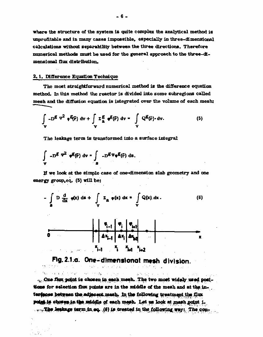
Fig. 2.1.a. One-dimensional mesh division.

,L One flux point i s chosen in each mesh. The two most widely used posi­tions for selection flux points are in the middle of the mesh and at the in-t«rft«*s between the adjacentmesh. In. the following treatment t h s Q m

pt^ i» ot^f^^t^ ad4dy» d ewh xa^h. Let us look at jnefh^oUrt i, .. WJ&? leakag* term in**. (9) Is treated in the following way: The con-

- 7 -

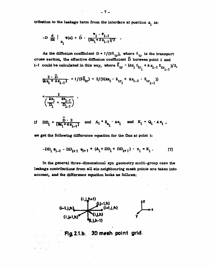
tribution to the leakage term from the interlace at position x. is ;

d . .,„, _ ^ f i " Vi Bx

I *(x) = D • *i

(A^+A^J/2 •

As the diffusion coefficient D = 1/(32 ), where t^ is the transport cross section, the effective diffusion coefficient D between point i and i-1 could be calculated in this way, where S = (Ax. Z^ + A x. , I . )/2,

^ ; Å x L _ 1 ) s , / ( 3 ^ ) - 2/(3(Ax. • X ^ + A V l • E ^ ) )

D - 2 1 1 P P i * ( o x ^ A x ^ , ) and A i ' U ^ - ax. and K. » Q. • Ax. .

we get the following difference equation for the flux at point i:

•DD.f^ - DDi+1 f i + 1 + ( V 0 0 ! * DD i+ l> ' V * l (7)

In the general three-dimensional xyz geometry multi-group case the leakage contributions from aU six neighbouring mesh points a re taken into account, and the difference equation looks as follows:

(i.LM) ij-1.h)

CWJ.H)

* J J M >

A. Fig, It.b. 3D mesh point grid.

. 8 .

6 D D X + < A £j .h + I DDS*f.ih-Kf,j.h-

n=l («)

where

Au.h"*vAY4v"f and

NG

4,g.h= A v * y j - A v ( 1 <Ef**' + x *• ^g,> **') • « g'*1

One such difference equation is necessary for each mesh point chosen. In order to solve the three-dimensional difference equation system (8),

3) an iteration scheme of the following form could be used '. The iterations are separated into inner and outer iterations. In the outer iteration the Bource distribution is calculated in accordance with equation (9). In the inner iterations the flux distribution is found on the basis of the previously determined source distribution. The inner iterations could be repeated until a certain convergence of the flux distribution is established.

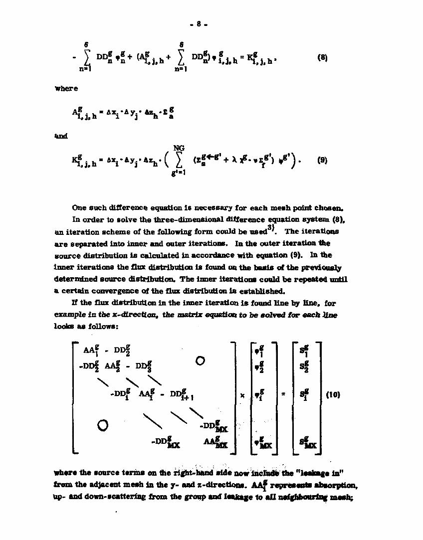
If the flux distribution in the inner iteration is found line by line, for example in the x-<Rreett<mt the matrix equation to be solved for each line looks as follows:

AAj - DD§

-DD| AAg - DD|

-DDf AAf - DDf+,

\ \ N

-DDf,

D DfdX

X

•T *f

*f

*SK

X

•f * !

*f 00)

where the source terms on the right-hand side now include the "leakage in" from the adjacent mesh in fhe y- and z-directions. AAf represents absorption, up- and down-scattering from the group and leakage to all neighbouring mesh;

- » -

DDf represents the leakage between mesh (i, j , h) and (i-1, j , h). The total number of mesh points in the x-direction is MX. The matrix equation (10) is solved directly by use of a forward eliminating and backward substituting method as described in refs. 4 and 5.

Bach outer iteration i s succeeded by an eigenvalue calculation which is set up by use of some sort of power method or a neutron balance equation

To speed up the convergence of the iterations numerous different methods have been used: alternating direction iterations, coarse-mesh re­balancing, overrelaxation ', extrapolation '. Common to all these methods is that several iterations are necessary. The number of necessary itera­tions is naturally dependent on the problem, but 25 iterations are a low estimate.

On a Burroughs B6700 computer each point iteration takes about 2 msec and for a 30 x 30 x 30 mesh problem two energy groups the computing time is at least 45 min.

The accuracy of difference equation calculations is rather problematic. In one dimension and one energy group, simple Taylor expansions of the flux could be used to get an estimate of the error introduced by the discretisation. Such investigations show that a mesh size not much greater than the free mean path is necessary, i . e. for light water reactors 2-3 cm. However, in three-dimensional calculations where the space i s divided into a three-dimensional grid also corner errors are introduced originating from the fact that only the six nearest neighbours are taken into account. Especially when small mesh sizes are used this could cause great errors. In the gen* eral case the problem is how great a mesh size it i s possible to use without introducing too great errors. Such answers only practical experiments can give. Several investigations seem to show that a mesh size of about 2 - 4 cm in the reactor and 2 cm in the reflector only introduces an error in the flux distribution of a few per cent and in the eigenvalue of a few per-wHl, for a typical light water reactor configuration when the mesh point i s chosen in the middle of the mesh.

Another difficulty in the difference equation technique is where to select the flux points: in the middle of the mesh or at the interface between the ad­jacent mesh. These two different discretisation methods should naturally in the limit with very small mesh sizes converge against the same result. In practical muW-dlmensional calculations with finite mesh size these two methods give different results, at worst quite different results. Which of the methods gives the most accurate result depends on the nature of the

- 1 0 -

problem. The method with flux points at the interfaces gives the most ac­curate determination of the leakage terms whereas the absorption and source terms are worse determined and vice versa.

Some practical experiments in this field have been performed by G. K. Kristiansen at the Reactor Physics Department at Risø . He has per­formed several two-dimensional xy geometry test calculations on a math­ematical example simulating a quarter of a reactor core, where two energy

71 groups were used. Two difference equation codes were used, DC4 ' with the flux points chosen at the interfaces and TWQDIM ' with the flux points chosen in the middle of the mesh.

On this mathematical example numerous calculations with these two codes have been accomplished with different mesh sizes. This was done to get an estimate of the discrepancy between discretisation methods used as a function of the mesh size.

The essence of these investigations is that the eigenvalue is rather well determined even in coarse-mesh calculations for both these codes, whereas the flux distribution is very sensitive to the mesh size used. For a calculation with 30 x 30 mesh the deviation between the results of the two codes was as much ad 10 per cent for thermal flux in the middle of the reactor core. For the thermal ftux peak in the reflector the results were even worse. It was not possible to get the deviation between the two codes below about one per cent even for calculations with 100 x i Q0 mesh, i. e.

4 10 mesh points in each energy group. As a two energy group calculation with 100 x 100 mesh takes about 1 i

hours on the Burroughs B6700 computer at Risø it is clear that three-dimensional calculations of so high an accuracy is impossible.

To compare different calculation methods for three-dimensional over­all calculations on light water reactors, a three-dimensional mathematical Benchmark Problem was set up *.

The intention with the Benchmark Problem was to set up a mathematical test example, which best possible simulates a quarter of a modern pressur­ised water reactor with varying enrichment zones and different insertion of the control rods. The reactor core was surrounded by a light water reflec­tor.

The Benchmark Problem was calculated by several three-dimensional code* from all over the world, both with difference equation codes and with approximate codes as e.g. nodal codes and flux syntheses codes. In advance of felting up the Benchmark calculation it was our hope that the dispersion of

- It -

the results from the exact difference equation codes would be less than those of the approximate codes« and in this way enable us to find out what was the right answer to the problem. Unfortunately, this was not the case; the devi­ations between the exact codes appeared to be just as great as those of the approximate codes, in the worst case about 2 per cent at the eigenvalue and 25 per cent at the thermal flux distribution inside the reactor core.

The conclusion of all these considerations concerning three-dimensional difference equation technique is that this exact technique is prohibitive. Exact, taken in the sense that the result moves towards the correct diffusion theory result as the mesh size decreases. Especially for calculations of repetitive nature, as for example overall burn-up calculations or void iterations« the cost in computing time on nowadays computers i s enormous.

From the previous considerations it is clear that some sort of approxi­mate method is necessary. By utilizing beforehand knowledge of the result of the problem in the form of experimental data, previous exact calculations on similar examples or two-dimensional calculations on the actual problem« it is possible to set up approximate calculation schemes which give better results than does a coarse-mesh difference equation calculation for the same consumption of computer time.

The two most significant approaches to approximate overall diffusion theory methods i s the nodal method and the flux synthesis method. These two methods are discussed in the following sections of this report.

2.2. Coarse-Mesh Methods

As menL*oned in the previous section one of the methods for speeding up multi-dimensional diffusion theory calculations is to modify the difference equation scheme to allow greater mesh. This reformulation could be done rigorously without taking advantage of any beforehand knowledge of the sol­ution of the specific problem by using for example polynomial expansions in­side the mefrh. Another type of coarse-mesh methods takes advantage of all sorts of beforehand knowledge of the specific problem in the form of experi­mental data or results from previous exact calculations on similar problems. The latter type of coarse-mesh approximation theory is normally called no­dal theory.

2.2,1. Nodal Theory

In the nodal theory one takes advantage of the fact that in a great modern light water reactor the different regions are only weakly coupled. The re-

- 1 2 -

actor ia divided into a coarse grid of nodes, in the horizontal plane properly one node per fuel box; further the calculations are facilitated by iterating on the source distribution instead of Hie multi-group flux distribution. The source terms in the nodes are linked together by some coupling coefficients. These coupling coefficients could be calculated more or less sopMsticatedly by use of one-group date or multi-group data. The neutron transport be­tween the nodes is then represented by the coupling coefficients. Common to the different methods for calculation of the coupling coefficients is the fact that the coupling coefficients are not universal, but require some problem-depending fitting parameters, g-factors, determined outside the nodal program.

2 .2 .1 .1 . The Flare Model One of the first and best documented nodal programs is the American program Flare . A brief survey of the methods used in this program is given here to illustrate the principles of the nodal model.

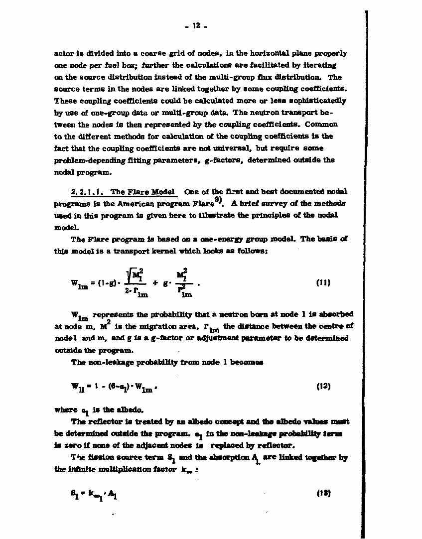
The Flare program is based on a one-energy group model. The basis of

this model is a transport kernel which looks as follows:

1111 2. r. rr * r l m ^ m

W, represents the probability that a neutron born at node 1 is absorbed at node m, AT is the migration area, 1*^ the distance between the centre of nodel and m, and g is a g-factor or adjustment parameter to be determined outside the program.

The non-leakage probability from node 1 becomes

W u - 1 - ( « - « ! > ' W j ^ . (12)

where «u i s the albedo. The reflector is treated by an albedo concept and the albedo values must

be determined outside the program, a. ia the non-leakage probability term is zero if none of the adjacent nodes is replaced by reflector.

Tte fission source term Sj and the absorption A are linked together by the Infinite multiplication factor km :

- 13 -

On the other hand, the absorption rate at node 1 can be written as:

6

V ISmWml+ hWW <"> m

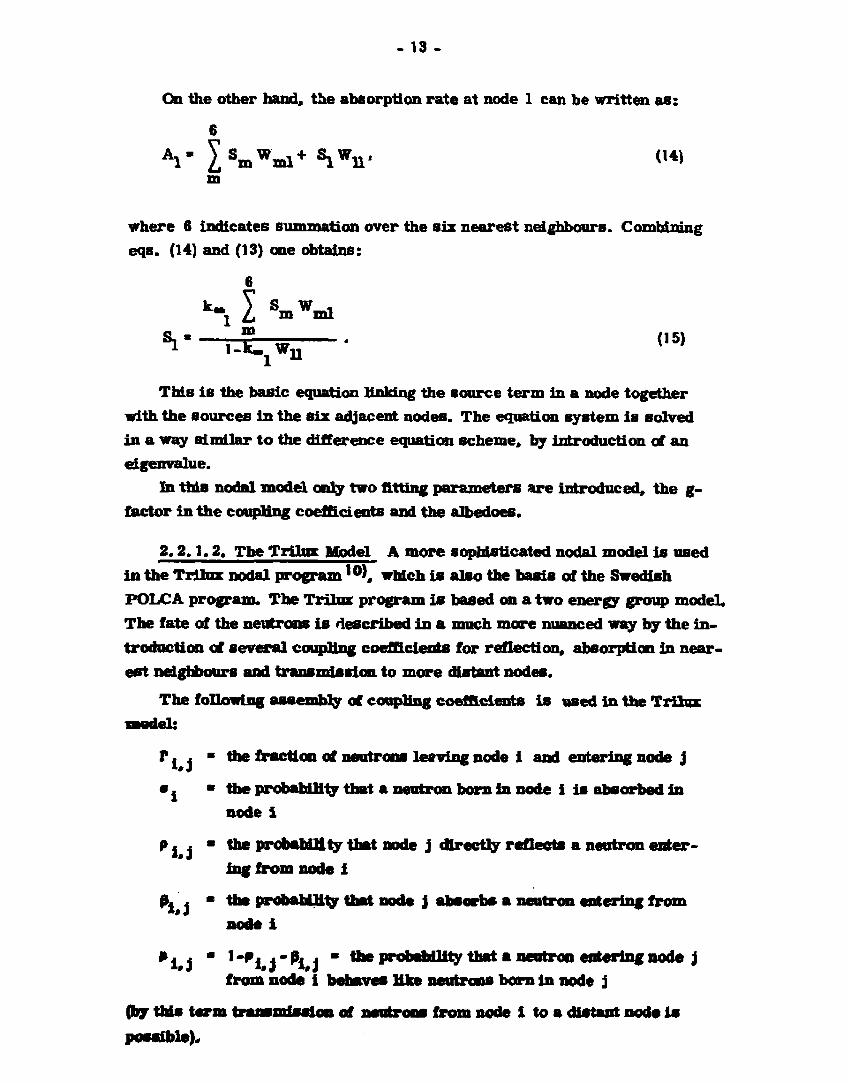
where 6 indicates summation over the six nearest neighbours. Combining eqs. (14) and (13) one obtains:

6

^ I S m W m l V i-k^w-n <,5)

This is the basic equation linking the source term in a node together with the sources in the six adjacent nodes. The equation system is solved in a way similar to the difference equation scheme, by introduction of an eigenvalue.

In tins nodal model only two fitting parameters are introduced, the g-factor in the coupling coefficients and the albedoes.

2 .2 .1 .2 . The Trilnx Model A more sophisticated nodal model is used in the Trilmc nodal program10), which i s also the basis of the Swedish POLCA program. The Trilnx program i s based on a two energy group model. The fate of the neutrons i s described in a much more nuanced way by the in­troduction of several coupling coefficients for reflection, absorption in near­est neighbours and transmission to more distant nodes.

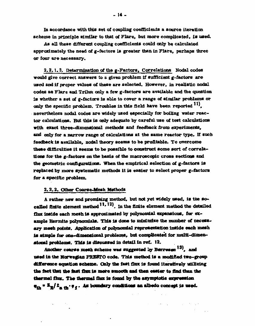
The following assembly of coupling coefficients i s used in the Trilux

P x j • the fraction of neutrons leaving node i and entering node j

• 4 * the probablUly that a neutron born in node i is absorbed in node i

P j x • the probability that node j directly reflects a neutron enter­ing from node 1

0£ * * the probability that node j absorbs a neutron entering from node i

* i i " ' • ' r j ' P i j " the prcbaWUty that a neutron entering node j from node 1 behaves like neutrons born in node j

(by this term transmission of neutrons from node i to a distant node Is possible).

- 1 4 -

Ih accordance with this set of coupling coefficients a source iteration scheme in principle similar to that of Flare, but more complicated, i s used,

As all these different coupling coefficients could only be calculated approximately the need of g-factors is greater than in Flare, perhaps three or four are necessary.

2.2.1.3. Determination of the g-Factors, Correlations Nodal codes would give correct answers to a given problem if sufficient g-factors are used and if proper values of these are selected. However, in realistic nodal codes as Flare and Trilux only a few g-factors are available and the question is whether a set of g-factors is able to cover a range of similar problems or only the specific problem. Troubles in this field have been reported ' ', nevertheless nodal codes are widely used especially for boiling water reac­tor calculations. But this i s only adequate by careful use of test calculations with exact three-dimensional methods and feedback from experiments, and only for a narrow range of calculations at the same reactor type. If such feedback i s available, nodal theory seems to be profitable. To overcome these difficulties it seems to be possible to construct some sort of correla­tions for the g-factors on the basis of the macroscopic cross sections and the geometric configurations. When the empirical selection of g-factors is replaced by more systematic methods it i s easier to select proper g-factors for a specific problem.

2.2.2. Other Coarse-Mesh Methods

A rather new and promising method, but not yet widely used, i s the so-called finite element method1 '*12*. In the finite element method the detailed flux inside each mesh is approximated by polynomial expansions, for ex­ample Hermite polynomials. This is done to minimize the number of necess­ary mesh points. Application of polynomial representation inside each mesh i s simple for one-dimensional problems, but complicated for multi-dimen­sional problems. This Is discussed in detail in ref. 12.

Another coarse mesh scheme was suggested i y Berresen ', and used in the Norwegian PRESTO code. This method is a modified two-group difference equation scheme. Only the fast flux i s found iterettVely utilizing the fact that the fast flux i s mere smooth and then easier to find than the thermal flux. The thermal flux i s found by the asymptotic expiessluu * n " S B S £ S lb* "f * ** DOqnd*py conditions an albedo concept i s used.

- 1 5 -

2.3. Flux Synthesis Methods

Another approach to approximative three-dimensional flux distribution calculations is the flux synthesis method. In the flux synthesis method the number of flux points i s not minimized, but the fact that in many practical reactor calculations a certain separability between the vertical and the horizontal fluxes exists is utilized.

The three-dimensional flux distribution is approximated by a product of a radial solution and an axial solution:

•gC*.y»*) » fgC*.y)• • e(»). (is)

where (x, y) represents the radial direction and (z) the axial direction.

2 .3 .1 . Ordinary Flax Synthesis

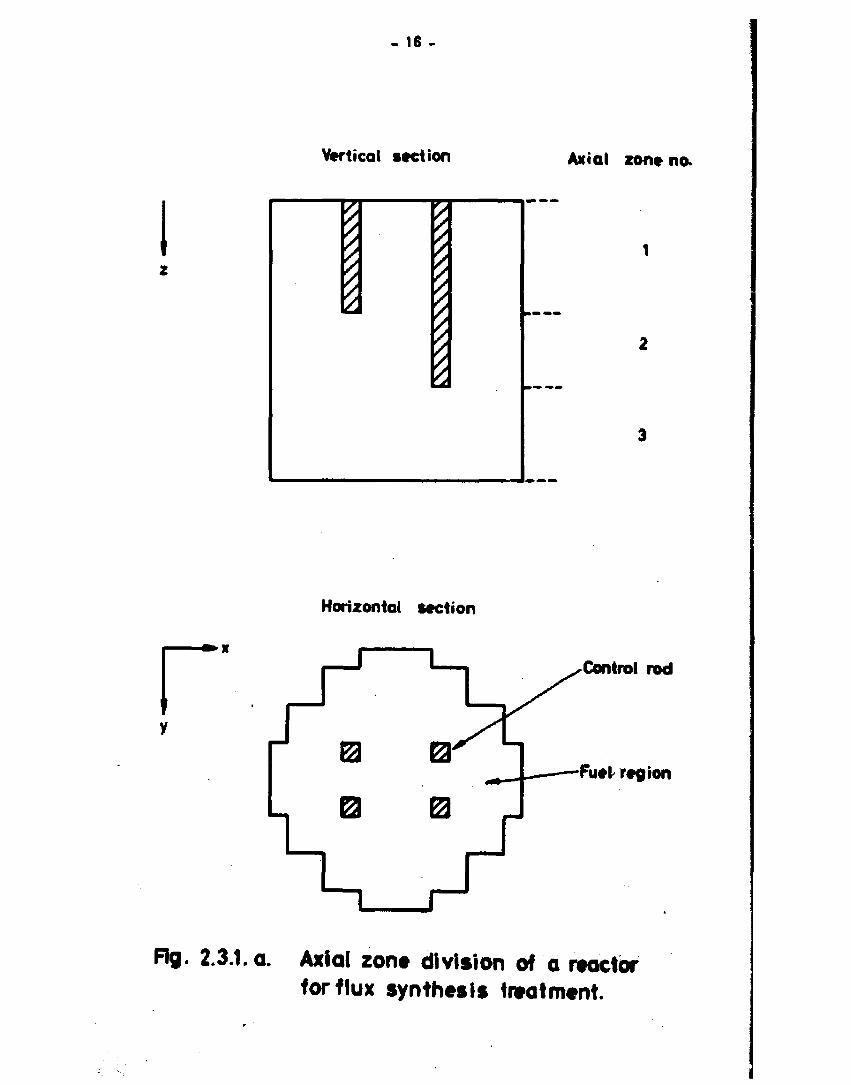
hi simple cases, for example a homogeneous cube, full separability exists between the radial and axial solutions. Numerous mathematical examples with the same properties could be constructed. But also in many realistic reactor calculations the assumption of separability between the vertical and the horizontal solutions is a good approximation. In pressurized water reactors with the control rods either fully inserted or fully withdrawn the flux distribution in the axial direction is well approximated by a sin(z). In such cases the overall calculations could be performed in only two di­mensions. In the general case, without full separability between the flux solutions in the vertical and the horizontal directions, it is often possible to divide the reactor into some axial zones with no material variations in the axial direction in each zone. In fig. 2.3.1.a. a reactor configuration with some partially inserted control rods is shown. If the unrodded fuel zone is treated as a homogeneous medium, this reactor could be divided into three axial sones on the basis of the control rod positions. In each of these axial zones a two-dimensional difference equation calculation could be per­formed. By use of these radial flux soluttcae fhzz'Weigh^ed cross sections and radial leakage terms are calculated in each axial zone. On the basis of these effective cross sections a one-dimensional vertical calculation is per­formed. The three-dimensional flux distribution i s then simply predicted in the following way;

•*(*.*,*) • •*(*>• ?fC*,y). (17)

- 16 -

Vertical section Axial zone no.

Horizontal section

r Control rod

Fuel region

Fig. 2.3.1. a. Axial zone division of a reactor for flux synthesis treatment.

- 17 -

where t f (x,y) ie the radial flux solution belonging to the different axial zones, and v*(z) is the one-dimensional vertical solution.

The radial flux distributions used are normally called trial functions. On the basis of the one-dimensional flux solutions axial leakage terms could be calculated for each axial zone to give suitable axial buddings for the trial function calculations. Iterations between the axial and the radial cal­culations could be established. This "stack" synthesis method described here is the classical single channel flux synthesis method, compare ref. 14. Synthesis programs based on this method have been used widely by, for example. General Electrics.

An extension of this method is the multi-channel flux synthesis meth -od '. In this method the reactor is divided into some vertical channels besides the axial zones. A one-dimensional flux calculation is performed in each channel. A rather complicated scheme for the leakage coupling be­tween the different channels and the different trial function calculations is used.

2. 3.2. Variational Flux Synthesis

In the variational flux synthesis the radial flux distribution at each vertical point is found by combining some precalculated trial functions to give the actual flux shape. The foundation of this method is described in ref. 16. The three-dimensional flux distribution is given by the following expansion:

?g(x.y,z) = Y 2£(z).HJ[<x,v) . (18) k^l

where

K • number of trial functions in group g

H*(x,y) • trial function number k in group g

z][ (z) • mixing function number k in group g.

The trial functions are radial flux distributions representative of the radial flux distribution throughout the reactor. The trial functions are as­sumed to be precalculated In advance of the synthesis calculation. At each z-pobrt the mixing functions represent the blending coefficients of the trial functions.

. 1 8 .

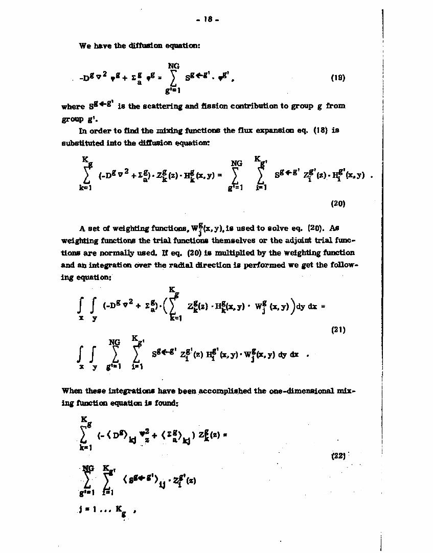
We have the diffusion equation:

NG . - D * * 2 t * + L f t g = £ S * < * ' . v « \ 09)

g-1

where S^*"g is the scattering and fission contribution to group g from group g'.

In order to find the mixing functions the flux expansion eq. (18) is substituted into the diffusion equation:

*g NG Kjf Y (-Dgv2+l|).z|(z)-H«(x,y)» V 2 SÉ^zfw.-lffe.y)

(20)

A set of weighting functions, W?(x,y), is used to solve eq. (20). As weighting functions the trial functions themselves or the adjoint trial func. tions are normally used. If eq. (20) is multiplied by the weighting function and ah integration over the radial direction is performed we get the follow­ing equation:

j j (-D*v2 + S f ) . ( £ Z«(z) -Hj[{*,y) * W« (x,y))dy dx = x y k*1

(21) NG ^g«

/ / 1 L s8^g'zf«2)^'^y)'W8(x,y)dydx . x y g'*1 i«1

When these integrations have been accomplished the one-dimensional mix-ing function equation is found;

I k-l

i*<-<I^>«^+<I!(>kj'zfw-

s«1 (22)

2 Y <««^g,>ir2f,(z) gi«l i«i

J " l . . . Kg ,

- 19 -

where { D* >.. is the diffusion constant radially integrated by trial function number k and weighting function number j in group g. The integrated term, (E*») , is now inclusive of the radial leakage term D* v . The source

term is integrated by trial function number i in group g1 and weighting function number j in group g.

Eq. (22) i s the basic equation to be solved in order to find the mixing functions Z?(z). The equation system is in principle one-dimensional, but it is more complicated than the one-dimensional difference equation; approx­imately K x K terms are to be handled for each space point. Moreover the trial and weighting fraction integration is rather complicated and time consuming, especially the computation of the radial leakage terms. The flux synthesis method described above is normally called variational single channel flux synthesis with continuous trial functions, i. e. the same set of

trial functions are used throughout the whole reactor. Several computer pro-5 17 181 grams have been constructed on the basis of this method ' * '.

An obvious extension of the method is to allow different sets of trial functions to be used in the different axial zones. This method is called vari-

19 201 ational flux synthesis with discontinuous trial functions * '. The mixing function equation is further complicated by the discontinuities and discus­sions are still going on about the coupling between the different axial zones. Another extension of the variational synthesis method is to use it for multi­channel flux synthesis, but this method is so complicated that the straight­forward ordinary three-dimensional difference equation technique is more advantageous.

2.4. Discussion of the Different Approximative Methods

In order to choose the approximative method which best fulfils the re­quirement for three-dimensional overall calculations at Risø the following arguments must be taken into account. For calculations on a selected re­actor for which lots of measurements are available the nodal method and the other coarse mesh methods may give good results. However, for cal­culations on different reactor types with only few measurements available this method seems less attractive. The variational flux synthesis method Is a more straightforward extension of the two-dimensional difference equation method, but naturally it is a drag that there is no possibility for taking advantage of available measurements. The method with discontinuous trial functions i s mathematically complicated and time consuming and it is

. 2 0 .

difficult to predict which trial functions ought to be used, and where. For these reasons the variational single channel flux synthesis method was chosen as the method which best fits the type of calculations normally per­formed at Risø.

- 2 1 -

3. THE THREE-DIMENSIONAL FLUX SYNTHESIS PROGRAM SYNTRON

As mentioned in the previous chapter, the variational single-channel flux synthesis method has been selected as the approximative method best suited for the type of calculations usually performed at Risø. Based on this method a computer program called SYNTRON has been constructed. Originally the program was written for the IBM 7094 computer at NEUCC, compare ref. 5. Later the program has been converted for the Burroughs B67O0 computer at Rise. In addition the program has been extended by dif­ferent criticality search options. In this chapter a survey of the main fea­tures of the program is given.

3.1. The Principles for the Construction and the Solution of the Flux Synthesis Equation

The flux synthesis program SYNTRON is described in detail in ref. 5. Here only a survey of the main principles for the construction and the sol­ution of the flux synthesis equation is given. A flux synthesis calculation could be divided into three main parts: the generation of a suitable set of trial functions; the construction of radially-integrated cross sections and leakage terms and thereby the construction of the matrix elements for the synthesis equation; and last the solution of the synthesis equation to give the mixing functions and the eigenvalue.

The trial functions and the weighting functions are calculated by use of ordinary difference equation technique. The Onx point is chosen in the middle of the mesh. The routine used for the calculaticn of these functions is de­scribed later in this report.

In section 2.3.2, equation (22Vthe mixing function equation,, i s shown. The coefficients in this equation consist of radially integrated cross sections and leakage terms. The cross sections are just integrated weighted by the trial and weighting functions. As an example the absorption cross section integration looks as follows

AkVz)* / /ES-Hk^'y>-wf^y>dxdy • <23)

y *

The index (z) Indicates that the integration ought to be performed at each axial flux point. In principle the integration of the diffusion coefficients and of the scattering cross sections i s performed in the same fashion.

- 2 2 -

The calculation of the radial leakage term, called DBZf(z), is more complicated as the ^ operator is involved. The leakage term is calcu­lated by the following expression:

DBZ*.(z)= J J DS.W«(x iy).V^ y l^{x,y)dxdy . (24)

y x

It ought to be mentioned that the coefficient ( £ * ) M i s inclusive of the

radial leakage term. i . e. defined as;

<£f>k j = A | j + D B Z ? i • <25>

How these integrations a re carried out in practice is described in ref. 5 One thing which can diminish the number of necessary integrations is the fac that only one set of integrations t s necessary for each axial sone. For the configuration shown in fig. 2 .3 .1 , a, for example, only three sets oi inte­grations are necessary even if perhaps 50 mesh points are used in the axial direction.

When the radial integrations are performed and thereby the Coefficients for the mixing function equation are found the problem is how to solve tids equation. The equation is in principle one-dimensionalj however, it is more complicated than the one-dimensional difference equation. Approxi­mately K x K points, where K is the number of trial functions in group g, are to be handled for each mesh point in the axial direction. The methods used for the solution of the mixing function equation in the SYNTRON prog­ram are described in ref. 5. Here only the structure of the matrix equation is discussed.

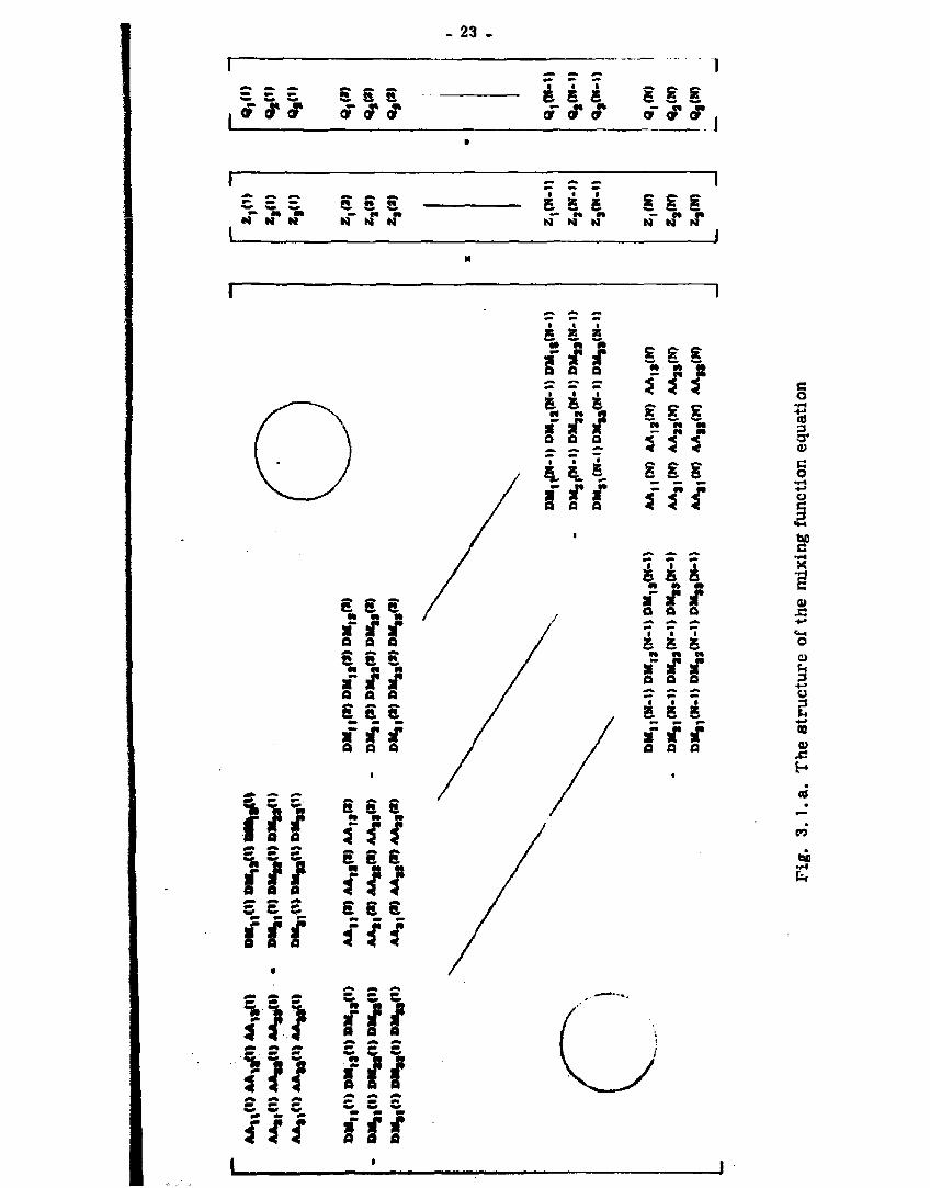
As described in ref. 5, equation (22) i s z-integrated to transform the equation into a difference equation system:

-BM ? (Z-1)-"Z*(S-1) + 3A"'(S)-<Z*(B) - DM*(s)-'Z*(*M) - Qg(z) ,

(26)

where

DMg(z-1) « a square matrix of the degree K x K representing

the leakage between mesh point z and %-\ and vice

versa

23

1 C S C

, * * *

1 £ S -S" «- *

1

III

m -

•

N

i i i S-Il

i i i N- ? f

i-Il,

!

m iff

m S £ S

m • i i

£ £ £ M n i?

* sT aT O O Q

* ~ i

rrr

m § § g

m 5 £ £

M M M

»-tf*-o a a • • i

£ £ S

*= ft a Q a

c o - i - i

-s 3 3* a? O

•r-l

C «w

bo c

I H X

4>

x:

o

o 3

m m m

m S £ S

Hi L

. 2 4 .

AA^(s) = a square matrix of the degree K * K representing the total absorption in mesh number % inclusive of radial and axial leakage out from the mesh

Q*<z) = a vector of the degree K representing the source terms at mesh number s

*Z *(z) * a vector of the degree K representing the values of the different mixing functions at mesh number z

As an illustration the full matrix equation to be solved i s shown in fig. 3. l .a for an example with three trial functions in each group. The group index is omitted as the structure i s the same in all groups. The num­ber of mesh points in the z-direction i s N. The square matrix is similar to that of one-dimensional difference equation technique, only the elements in the matrix equation are now submatrices. If the eigenvalue i s associated to the source terms, the left-hand side square matrix i s unchanged during the iterations. For that reason It iB possible to invert the diagonal submstrices once« before the iterations are started. The solntion method used, of. ref. 5, i s very fast compared to the cross section integration and the calculation of the trial functions. By s se ot this iteration scheme the different energy groups are linked together through the source terms. In order to solve the equation system it i s necessary to introduce an eigenvalue, for example the effective multiplication factor k ^ . The eigenvalue is calculated by an over­all neutron balance equation.

3,2. The Eigenvalue, Different CrittcaHty Options

Different criticaUty options are implemented in the SYNTBON program. An eigenvalue X could be associated to the production cross section » £_ In this way the system is held critical artificially and the effective multipli­cation factor kg« i s found as l/X. lforeover,it i s possible to associate an eigenvalue X to a macroscopic poison cross section t and in this way find the critical poison distribution in the reactor core. These two methods are standard methods well suited for both flux synthesis and difference equation technique.

The special flux synthesis treatment is utilized for the calculation of the critical dimensions in the axial direction. The method for direct iter­ation on the dimensions i s described in ref. 21. Two dimension control search option« are implemented; one for iteration on the dimensions and

- 25 -

one for internal boundary displacement with fixed outer dimensions (control rod movement). For these dimension search jnethods an eigenvalue is as ­sociated to the length of the selected axial zones. With a fixed set of trial functions no repetition of the cross section integrations are necessary during the iterations; only a f w repetitions of the solution of the mixing function equation are necessary. However, as this solution routine is very fast the extra cost in computation time is modest.

3.3. The Selection of the Trial Functions

One of the main problems in the flux synthesis is how to select the trial functions. No definite answer can be given to this problem. The SYNTRON program is not bound to use any fixed strategy for the generation of a proper set of trial functions. However, in most cases the trial func­tions are generated in the following way: characteristic axial zones are selected and two-dimensional difference equation calculations are performed on each of these zones. If the structure of the reactor configuration is com­plex it may be difficult to select such characteristic axial zones. It is neces­sary to restrict the number of trial functions as the flux synthesis method i s only favourable in comparison with tbe ordinary three-dimensional difference equation technique if only a few trial functions are used in each energy group (less than about 6). One thing which can diminish the number of trial function calculations - for calculations of a repetition nature - i s that the same set of trial functions may be used for several synthesis calculations.

In the SYNTRON program it is possible to use two different sets of weighting functions: the trial functions themselves or the adjoint trial func­tions. Normally the trial functions themselves are used,a£. the extra accuracy gained by using the adjoint functions is modest in comparison with the corn-outer time used for the calculation of the adjoint functions.

One thing which ought to be mentioned is that the set of trial functions used must be linearly independent. If this is not the case, the matrix equation will be singular. In the SYNTRON program it is left to the user of the prog­ram to construct a linearly independent set of trial functions.

S. 4. The Calculation of the Trial Functions

As previously mentioned the SYNTRON program is self-supplying with trial functions. In the program a two-dimensional difference equation routine is Included. The difference equation routine is to a certain degree analogous to the TWODIM program described in ref. 3. The flux point is chosen in the

. 2 6 .

middle of the mesh. The line-difference technique i s used. However, the difference equation routine in SYNTRON i s restricted to xy geometry as this is the only geometry of interest tor the synthesis calculations. To speed up the convergence of the iterations an extrapolation technique simi­lar to that of TWODM i s used. Furthermore,a simple line-overrelaxation technique is implemented. The boundary conditions may either be represented as extrapolation lywgfl« or gamma-matrices. The routine calculates auto­matically the adjoint trial functions if the method of adjoint weighting func­tions is chosen. Two criticality methods are implemented: k— and crit­ical poison distribution. The trial function calculation starts with a guessed flux distribution or with the previous trial function calculated on the same configuration if the trial function calculations are repeated. The calculated trial functions are stored on a disk file to be used in later synthesis calcu­lations.

3.5. Static Test Calculations

Several test calculations have been performed with the SYWTRON prog­ram to check the code and to estimate the error introduced by the synthesis approximation. Such calculations have been performed in two as well as three diinensions.

In ref. 5 a three-dimensional two-group test example is reported cal­culated both by SYWTRON and by the three-dimensional difference equation code wnirlaway \ WMrlaway takes the flux point at the interface between the mesh. The number of mesh points used was only 15 x 15 x 15, The size of the problem was determined by the capacity of Whirlaway on the IBM 7094 computer at NEtJCC. However, since the geometry of the test problem was rather simple the agreement between the results appeared satisfactory.

Some two-dimensional test calculations are presented in ref. 21. A comparison was made between two-dimensional SYWTRON synthesis calculation and SYNTRON difference equation calculations. Mb discretisation errors were involved in this comparison tm the discretisation method used was the same in both calculations; moreover, fine-mesh calculations were possible. Both k̂ jy search calculations and control search (internal boundary displacement) calculations were performed. In both cases an acceptable agreement between the results was observed.

In the thrne-dimensional international Benchmark Problem ' a comparison was made between several three-dimensional codes from all over the world. The Benchmark Problem simulates a quarter of a light water reactor with

- 27 -

varying enrichment sones and different insertion of the control rods. Al­though the dispersion in the results obtained by the different codes was great, the agreement between the SYNTRON results and the results ob­tained by the three-dimensional difference equation codes using the same discretisation method was excellent. The conclusion may be that the syn­thesis error, for this special case, is less than the discretisation error.

In appendix A to this report a test example is shown calculated both by the difference equation code DC4 ' and by SYNTRON. However, from these calculations it is impossible to get an acceptable estimate of the synthesis error as different discretisation methods are used in the two codes.

The conclusions drawn from these investigations may be that it is difficult to get an acceptable estimate of the synthesis error as exact three-dimensional fine-mesh dUference equation calculations are very expensive and in fact almost impossible on most computers. Comparisons between measurements and synthesis calculations could neither give a definite esti­mate of the synthesis error, as the errors from the cross sections and the box calculations are involved. However, naturally it is encouraging that the effective multiplication factors calculated by SYNTRON for the differ­ent start-up situations of the DRESDEN 1 reactor ' do agree quite satis­factorily with the measured ones.

The conclusions drawn concerning the applicability of the flux synthesis method are that for a wide range of reactor calculations the errors intro­duced by the flux synthesis approximation are less than the errors intro­duced by using coarse-mesh difference equation calculations consuming the same amount of computer time. For all the test calculations discussed above the SYNTRON calculations were about 10 times faster than the equiv­alent difference equation calculations. Naturally the synthesis method ought not to be used unrestrainedly as a bad set of trial functions introduces fur­ther errors. For very complicated configurations the difference equation technique ought to be used.

- 2 8 -

4. THE SYNTRON/VOID BURN-UP PROGRAM

m order to perform three-dimensional overall burn-up calculations the flux synthesis program SYNTRON has been extended to include the following facilities: cross section interpolation in a precalculated cross section library, burn-up treatment, and xenon transient treatment. Moreover, to be used for bailing water reactor calculations, routines for the calculation of the void and temperature distributions are implemented. In the following sections a brief description of the methods used in the different routines is given.

4.1. Cross Section Interpolation

For static SYNTRON calculations all regions are supplied with either macroscopic cross sections or boundary conditions. However, in the burn-up version of the program the burnable regions are supplied with macrosco­pic cross sections generated inside the program on the basis of an inter­polation in a cross section library constructed outside the program. The program is able to handle a cross section library tabulated as a function of a maximum of three parameters. Different libraries are allowed for the dif­ferent regions. The tabulation parameters may for example be? power density, burn-up and void fraction; or average void fraction during the burn-up« burn-up and actual void fraction. The actual cross sections for the different regions are simply determined by a linear interpolation In the cross section library. The cross section library is supposed to contain box average homogenized macroscopic cross sections calculated on the basis of detailed box calculations for example by use of the box program CDB '. In ref. 23 an example of. the construction of such a cross section library is shown. Different libraries may be used for different types <d fuel boxes, for example boxes with different enrichment or boxes with and without con­trol rod inserted. The cross section treatment described here is similar to that of the DBU program K

4.2. The Burn-up Treatment

For the burn-up treatment the reactor is divided into a number of burn-up regions. Each of the burn-up regions is- supplied with a set of interpolated macroscopic cross sections. On the basis of a detailed flux synthesis calculation, the energy released per fission and the total ther­mal power of the reactor, the average power density in the different burn-up

- 2 9 -

regions are calculated. The burn-up in the different regions is simply calculated on the basis of the following quantities: the average power den­sity, the uranium density and the tim« step length. When the power density is found the neutron flux is normalized for the use in the xenon calculations. In the coupled system the power density distribution is used as a basis for the void and temperature calculations. Moreover the power and burn-up distributions may be used for the determination of the cross sections for the next time step.

4.3. The Xenon Treatment

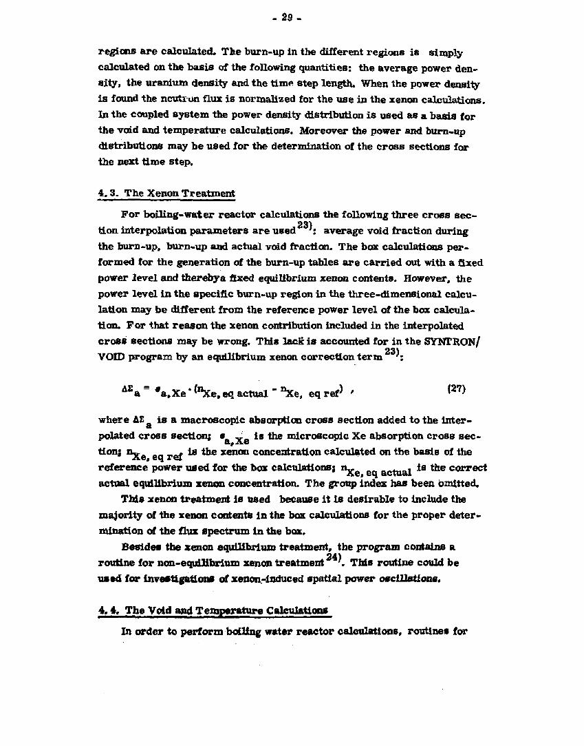
For boiling-water reactor calculations the following three cross sec­tion interpolation parameters are used ': average void fraction during the burn-up. burn-up and actual void fraction. The box calculations per­formed for the generation of the burn-up tables are carried out with a fixed power level and therebya fixed equilibrium xenon contents. However, the power level in the specific burn-up region in the three-dimensional calcu­lation may be different from the reference power level of the box calcula­tion. For that reason the xenon contribution included in the interpolated cross sections may be wrong. This lack is accounted for in the SYNTRON/ VOID program by an equilibrium xenon correction term ':

ASa = *a,Xe * fnXe, eq actual " "Xe, eq ref> ' ( 2 7 )

where AE is a macroscopic absorption cross section added to the inter-polated cross section; • „ . is the microscopic Xe absorption cross sec-Uon; i u . is the xenon concentration calculated on the basis of the

reference power used for the box calculations; n„ actual l s t h e c o r r e c * actual equilibrium xenon concentration. The group index has been omitted.

This xenon treatment is used because it is desirable to include the majority of the xenon contents in the box calculations for the proper deter­mination of the flux spectrum In the box.

Besides the xenon equilibrium treatment, the program contains a routine for non-equilibrium xenon treatment K This routine could be used for investigations of xenon-induced spatial power oscillations.

4.4, The Void and Temperature Calculations

In order to perform boiling water reactor calculations, routines for

- 3 0 -

2 the determination of the void and temperature distributions are implemented The void-temperature problem is treated as a multi-channel problem. The reactor is divided into a series of parallel channels, in the limit each fuel box is handled as a separate channel, butt usually more fuel boxes are com­bined and treated as one void channel. On the basis of the calculated power distribution and the hydraulic data of the core, the void routine calculates the axial void distribution in each channel and the temperature routine the axial temperature distribution, i. e. the moderator temperature, the cladding temperature and the fuel temperature distributions. In the present version of the routines the outer loop is neglected, i. e. the behaviour of the outer loop is determined by the inlet subcooling and the inlet total coolant flow. By use of such detailed void and temperature calculations the average void fraction and the average fuel temperature in each burn-up region are de­termined.

4.5. The Doppler Effect

The temperature varying most drastically throughout the reactor core is the fuel temperature. As mentioned in section 4 .3 . , the box calculations for the generation of the cross section library are performed at a fixed power level, and the 10-group cross sections for the pin-cells are calcu­lated at a fixed fuel temperature. To account for the local fuel temperature variations a Doppler correction treatment is implemented. The Doppler cor­rection treatment is only implemented for two-group calculations. The fast absorption cross sections and the removal cross sections taken from the

23) cross section library are adjusted by some polynomial expressions . The polynomial coefficients must be determined outside the program. The poly­nomials used are of the first degree for the burn-up and of the second de­gree for the void fraction. For the temperature dependence the standard square root term is used*

4.6. The Control Hod Treatment

No special control rod treatment is implemented in the SYNTRON pro­gram. As mentioned In section 4.1. different cross section libraries are al­lowed for the different burn-up regions, i. e. for example for fuel boxes with and without control rod inserted. For the generation of the cross sec-

j p h libraries box calculations are performed Willi and without control rod Inserted during the whole burn-up^ Thi« control rod representation is quite satisfactory for fuel boxes with the control rod in the same position during

- 31 -

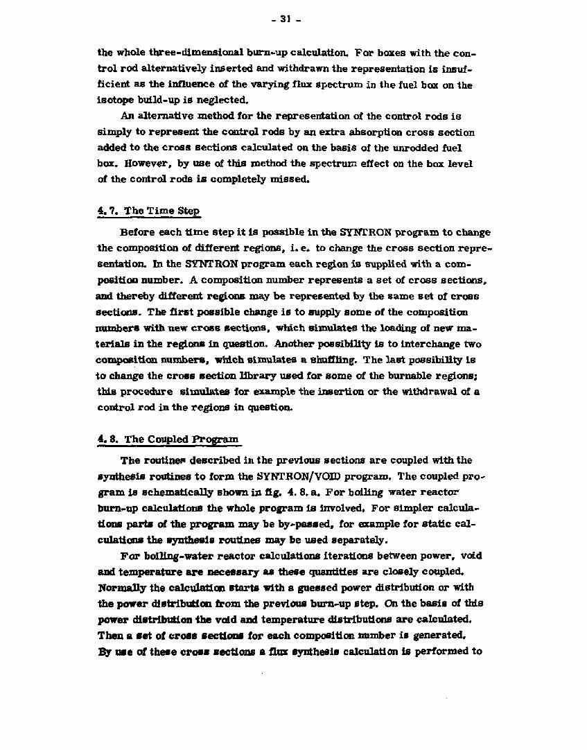
the whole three-dimensional burn-up calculation, For boxes with the con­trol rod alternatively inserted and withdrawn the representation is insuf­ficient as the influence of the varying flux spectrum in the fuel box on the isotope build-up i s neglected.

An alternative method for the representation of the control rods is simply to represent the control rods by an extra absorption cross section added to the cross sections calculated on the basis of the unrodded fuel box. However, by use of this method the spectrum effect on the box level of the control rods i s completely missed.

4. 7. The Time Step

Before each time step it i s possible in the SYNTRON program to change the composition of different regions, i . e. to change the cross section repre­sentation. In the SYNTRON program each region is supplied with a com­position number. A composition number represents a set of cross sections, and thereby different regions may be represented by the same set of cross sections. The first possible change is to supply some of the composition numbers with new cross sections, which simulates the loading of new ma­terials in the regions in question. Another possibility is to interchange two composition numbers, which simulates a shuffling. The last possibility is to change the cross section library used for some of the burnable regions; this procedure simulates for example the insertion or the withdrawal of a control rod in the regions in question.

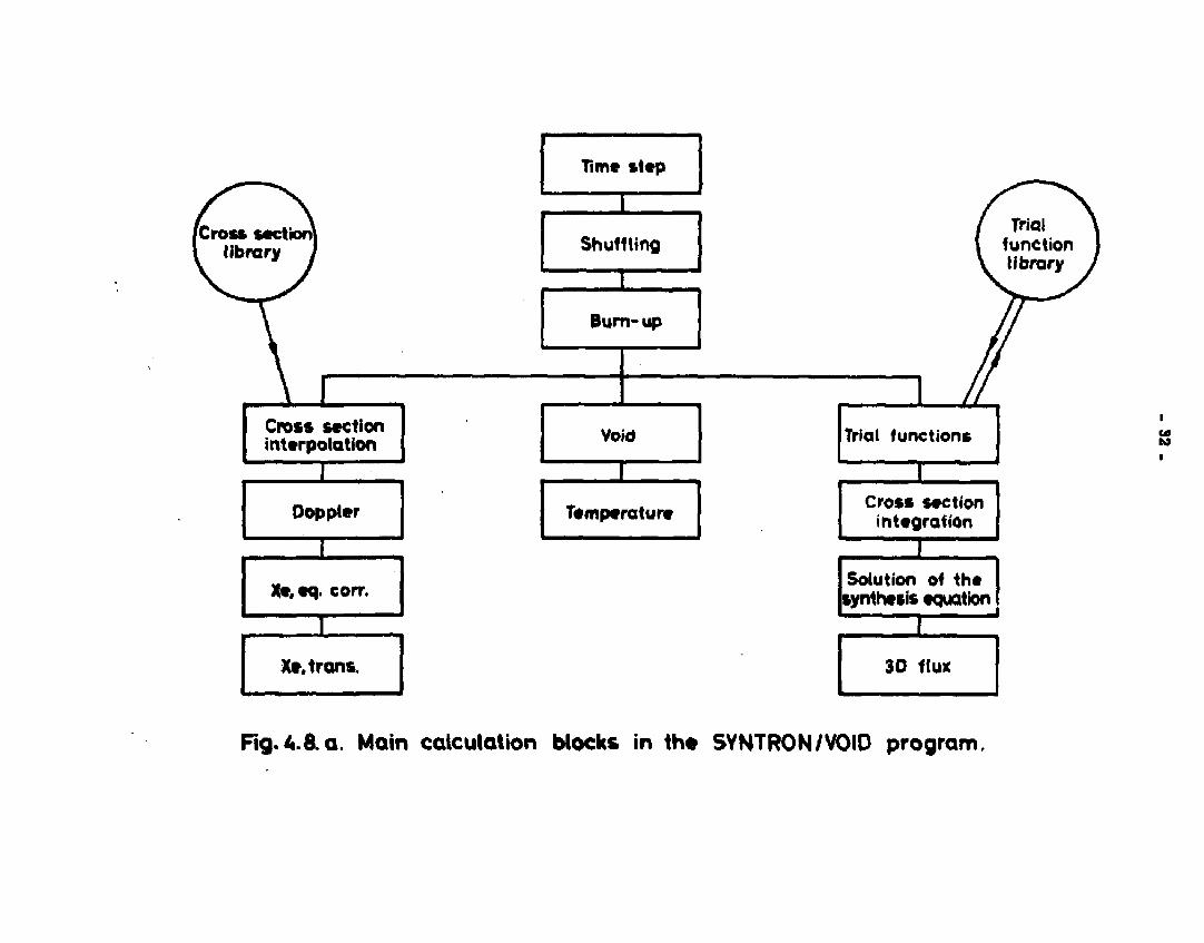
4.8. The Coupled Program

The routine*« described in the previous sections are coupled with the synthesis routines to form the SYNTRON/VOID program. The coupled pro­gram is schematically shown in fig. 4. 8, a. For boiling water reactor burn-up calculations the whole program i s Involved, For simpler calcula­tions parts of the program may be by-passed, for example for static cal­culations the synthesis routines may be used separately.

For boiling-water reactor calculations Iterations between power, void and temperature are necessary as these quantities are closely coupled. Normally the calculation starts with a guessed power distribution or with the power distribution from the previous burn-up step. On the basis of this power distribution the void and temperature distributions are calculated. Then a set of cross sections for each composition number is generated. By use of these cross sections A flux synthesis calculation is performed to

i section] f«sry J

Cross section interpolation

1

Doppler

i

Xe, eq. corr.

1

Xe, trans.

Time step

1

Shuffling

I

Bum-up

Void

1

Temperature

Trial functions

I Cross section

integration

1 Solution of the synthesis equation

1

3D flux

Trial function library

Fig.A.8.a. Main calculation blocks in the SYNTRON/VOID program.

CO

"S

get a new flux and power distribution. This scheme is repeated until the system is converged. Convergence criteria are put on the power distri­bution, the void distribution and the k „. When the system is converged changes in the cross section representation of different regions may be performed and a new burn-up step may be taken; if this is the case the burn-up distribution and the average void fraction during the burn-up for the different regions are calculated. Then again iterations between void, power and temperature are performed and so on.

A strategy for the calculations of trial functions must be decided. The necessary number of trial functions may be calculated once at the begin­ning of the burn-up calculation, or a new set of trial functions may be cal­culated at the beginning of each burn-up step. Finally the trial functions may be recalculated for each flux synthesis calculation during the void-power iterations. Naturally the previous trial functions are used as start guess for the recalculations.

For the DRESDEN 1 calculations ' the strategy of calculation of a new set of trial functions at the beginning of each burn-up step was used. However, in the succeeding chapter it is demonstrated that it seems to be more favourable to recalculate the trial functions continuously.

Experience has shown that it is of great importance for the convergence rate of the void-power iterations that some sort of underrelaxation is used in the coupling of void and power. In the following section of this report this is demonstrated by an example.

4.9. Optimal Calculation Strategy

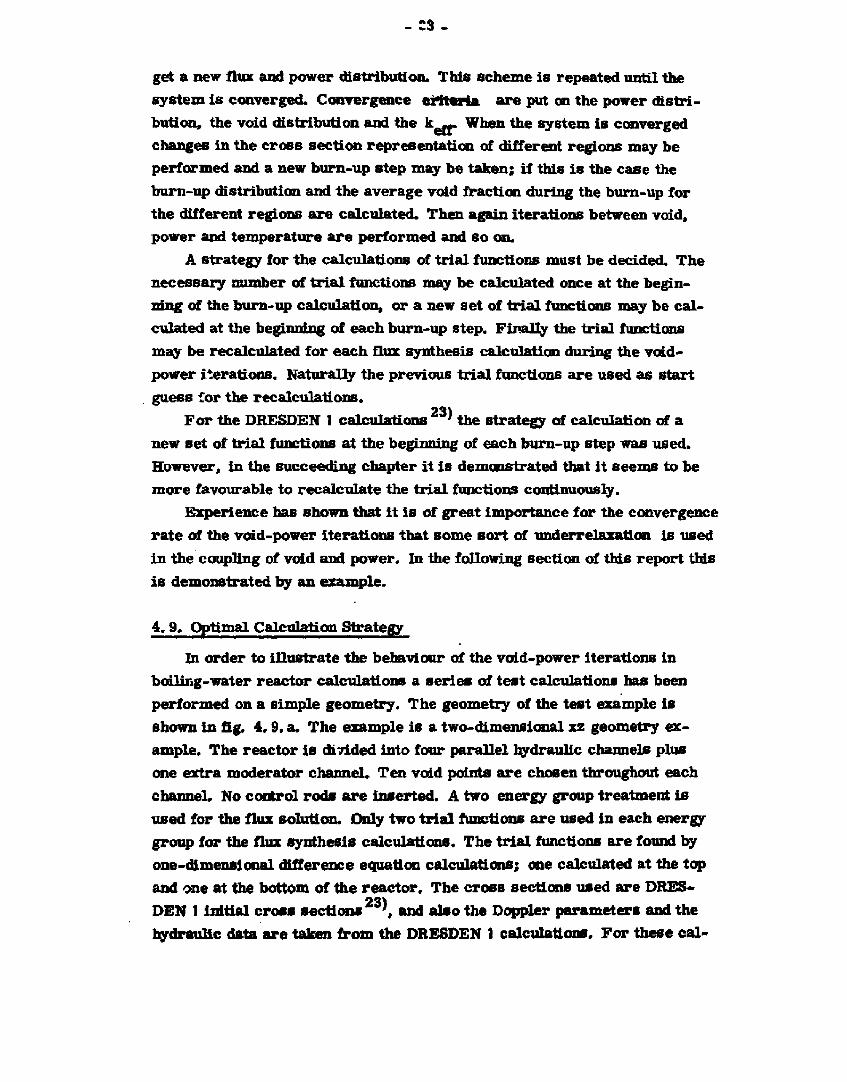
In order to illustrate the behaviour of the void-power iterations in boiling-water reactor calculations a series of test calculations has been performed on a simple geometry. The geometry of the test example is shown in fig. 4.9. a. The example is a two-dimensional xz geometry ex­ample. The reactor is divided into four parallel hydraulic channels plus one extra moderator channel. Ten void points are chosen throughout each channel. No control rods are inserted. A two energy group treatment is used for the flux solution. Only two trial functions are used in each energy group for the flux synthesis calculations. The trial functions are found by one-dimensional difference equation calculations; one calculated at the top and one at the bottom of the reactor. The cross sections used are DRES­DEN 1 Initial cross sections \ and also the Doppler parameters and the hydraulic data are taken from the DRESDEN 1 calculations. For these cal-

- 3 4 -

culations the power density and the total mass flow are adjusted to give a reasonable outlet void fraction. For the flux solution 55 mesh points are used in the x-direction and 36 mesh points in the z-direction, the synthesis direction.

2(cm) J°P r»ftector (~ 50»/. void)

295 285

Symmetry plane—»•

Reactor core divided into 4 parallel channels

K>

Reflector (0*/. void)

•-x(cm)

Reflector (0*/. void)

Fig. A.9. a. Test reactor, description.

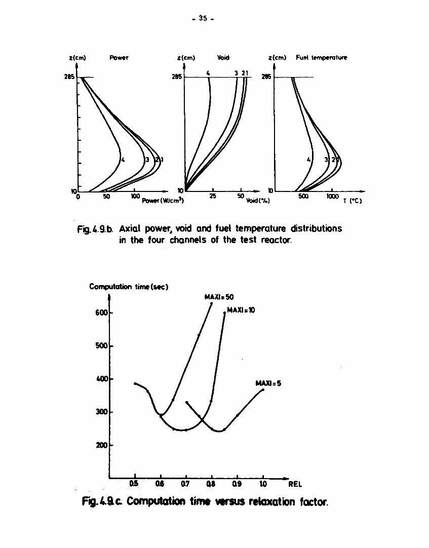
In fig. 4. 9, b. the calculated axial power, void and fuel temperature distributions in the four channels are shown. The total form factor was found to be 2. 01. The power, void and fuel temperature are highest in channel no. 1 and lowest in channel no. 4, as expected.

Several calculations on the example have been performed in order to find the optimal calculation strategy. The method of continuous recalcula­tion of the trial functions was used, i. e. new trial functions were calculated for each void-power iteration. The influence on the computation time neces­sary for the whole calculation of the following two quantities was investi­gated: the value of the power underrelaxation factor REL; the degree of convergence of the trial function calculations and the flux synthesis calcu­lation at each void-power iteration, i. e. the maximum number of iterations, MAXI, allowed for each flux solution. In fig. 4.9. c.the total computation time for the problem versus the value of the relaxation factor for different degrees of convergence of the flux solutions i s shown. It is seen that for

- 35 -

z(cm) Power

285

2 (cm) FwM temperature

10

14 13 VU

50 100 Power (W/cm3) Void(*/.)

500 1000 T CC)

Fig.4.9b. Axial power, void and fuel temperature distributions in the four channels of the test reactor.

Computation time (sec)

600

500

400

300

200

MAXI=50

MAXI s 10

MAXI=5

I i ' ' L 05 06 07 at 0.9 U> REL

Fig.4.&c Computation timt versus relaxation factor.

- 8 6 -

05 06 07 08 0.9 1J0 REL

Fig.4.9.d. Optimal rekixation factor versus the degree of convergence of each iteration.

Form factor

2.50

2.00

150 •

High relaxation factor

10 Iteration no.

Fig.49.e. The form factor as a function of the iteration number fat/ oVfltnwt retaxatioo factors,

- 37 -

each value of MAXI an optimal underrelaxation factor is found. Calcula­tions with MAXI = 2 were also performed, but these calculations were very slow as lots of void-power iterations were necessary; a relaxation factor greater than one seems to be favourable. The power convergence criterion

-3 in all these calculations was 10 .

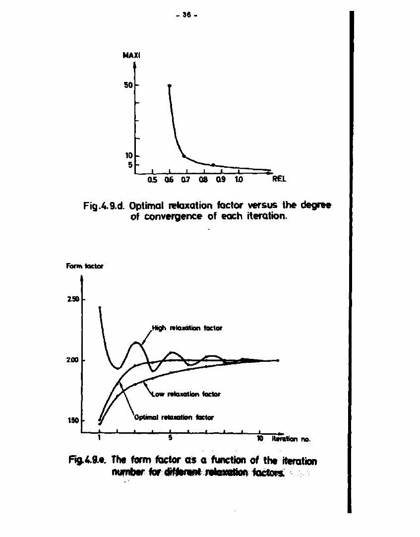
The calculation with MAXI equal to 50 represents nearly full convergence of the flux calculations at all void-power iterations. These investigations show that full convergence of all flux solutions demand a low underrelaxa­tion factor, whereas a loose convergence of the flux solutions only demand a weak underrelaxation. In fig. 4. 9. d. the optimal relaxation factor versus the degree of convergence of the flux solutions i s shown. The convergence of the power distribution represented by the form factor during the void-power iterations i s shown in fig. 4. 9. e. For the high relaxation factor damped oscillations are observed.

The most favourable calculation strategy seems to be to use a loose convergence criterion for the flux solution, MAXI about 5, and a slight underrelaxation on the power. Full convergence of all flux solutions i s less attractive as this method is slower and very sensitive to the relaxation factor used.

Calculations with a fixed set of trial functions for all void-power iter­ations were likewise carried out. However, this method is more sensitive to the selection of the trial functions and not much faster than the method of loose convergence of the flux solution.

4.10. Calculations Performed with the SYMTRON/VOIP Program

A two-dimensional burn-up calculation without void has been performed 211

in order to check the accuracy of the flux synthesis method ' . T h e test ex­ample was calculated both by SYNTRON and the difference equation burn-up program DBU \ which has a burn-up treatment equivalent to that of SYN­TRON. The problem was calculated by use of different numbers of recalcu­lations of the trial functions during the burn-up, and both with and without adjoint trial functions. Only k . , versus the average burn-up was calcu­lated. The accuracy of the synthesis calculations was found to be satisfactory if the trial functions were recalculated once during the burn-up.

The SYNTRON/VOID program has been used for calculations on the DRESDEN 1 reactor '. No estimate of the synthesis error was possible as no accurate three-dimensional program was available. However, the calculated effective multiplication factors for different configurations of the

- 3 8 -

cycle 1 of the reactor do agree satisfactorily with the measurements. The errors observed in the calculated power distribution and the exposure distribution at the end of cycle 1 originate from both the synthesis error, the limited number of hydraulic channels used and the fact that only quarter core calculations were performed.

- 39 -

5. SUMMARY

The conclusions of these investigations regarding the approximative solution of the three-dimensional diffusion equation are: for a wide range of reactor calculations the variational flux synthesis method is favourable. The errors introduced by the flux synthesis approximation are typically less than the errors introduced by similar coarse-mesh difference equation calculations consuming the same amount of computation time. Naturally it is a drag for the synthesis method that there are no possibilities for taking advantage of available measurements. For calculations on one selected re­actor for which lots of measurements are available the nodal method may give better results. However, for calculations on different reactor types with only few measurements available this method seems less attractive than the synthesis method.

- 4 0 -

APPENDDC A

TEST EXAMPLE FOR COMPARISON BETWEEN DC4 AND SYNTRON

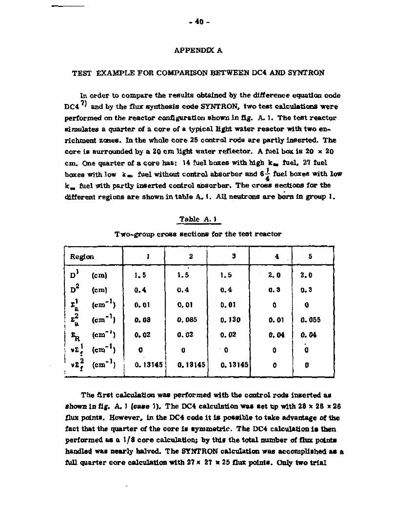
In order to compare the results obtained by the difference equation code DC4 ' and by the flux synthesis code SYNTRON, two test calculations were performed on the reactor configuration shown in fig. A. 1. The test reactor simulates a quarter of a core of a typical light water reactor with two en­richment zones. In the whole core 25 control rods are partly inserted. The core is surrounded by a 20 cm light water reflector. A fuel box is 20 x 20 cm. One quarter of a core has: 14 fuel boxes with high k„ fuel, 27 fuel boxes with low kno fuel without control absorber and 6-7 fuel boxes with low k„. fuel with partly inserted control absorber. The cross sections for the different regions are shown in table A. 1. All neutrons are born in group 1.

Table A. 1

Two-group cross sections for the test reactor

Region

D1 (cm)

D2 (cm)

Xl (cm"1 .

4 (cm"1)

^ (cm"')

vc j (cm"1)

v£j (cm -1)

1

1.5

0.4

0.01

0.08

0.02

0

1 0.13145

i

2

1.5

0.4

0.01

0.085

0.02

0

| 0.13145

3

1.6

0.4

0.01

0.130

0.02

0

0.13145

4

2.0

0.3

0

0.01

0.04

0

°

5

2.0

0.3

0

0.055

0.04

0

° The first calculation was performed with the control rods inserted as

shown in fig. A.1 (case 1), The DC4 calcuLation was set Up with 28 x 28 x 26 flux points. However, in the DC4 code it is possible to take advantage of the fact that the quarter of the core is symmetric. The OC4 calculation is then performed as a 1/8 core calculation; by this the total number of flux points handled was nearly halved. The SYNTRON calculation was accomplished as a full quarter core calculation with 27 x 27 x 25 flux points. Only two trial

- 4 1 -

functions were used in each energy group. The trial functions were found by two-dimensional difference equation calculations: one at the upper rod-in zone, and one at the lower rod-out zone.

Next the initial calculation, the critical position of the control rods (the whole group) is calculated by use of SYNTRON, case 2. The method of internal boundary search was used, see chapter 3 in this report. The criti­cal insertion of the control rods was found to be 269 cm, compare fig. A. 1. A DC4 calculation was then performed with the new control rod position. The number of flux points for this calculation was 28 * 28 x 31. in table A. 2 the calculated values of k , , and the computer time used are shown.

Table A. 2

^ ^ - - _ _

DC4 Case 1

SYNTRON

DC4 Case 2

SYNTRON

keff

1.0198

1.0170

1.0032

1.0000

Processor time (min)

35

6.1

45

6.5

Total time (min)

59

7.2

77

7.4

It might be mentioned that the computer times for the SYNTRON cal­culations are inclusive of trial function calculations and printing of the re­sults. The time used for the real synthesis calculation is only about 20% of the total time.

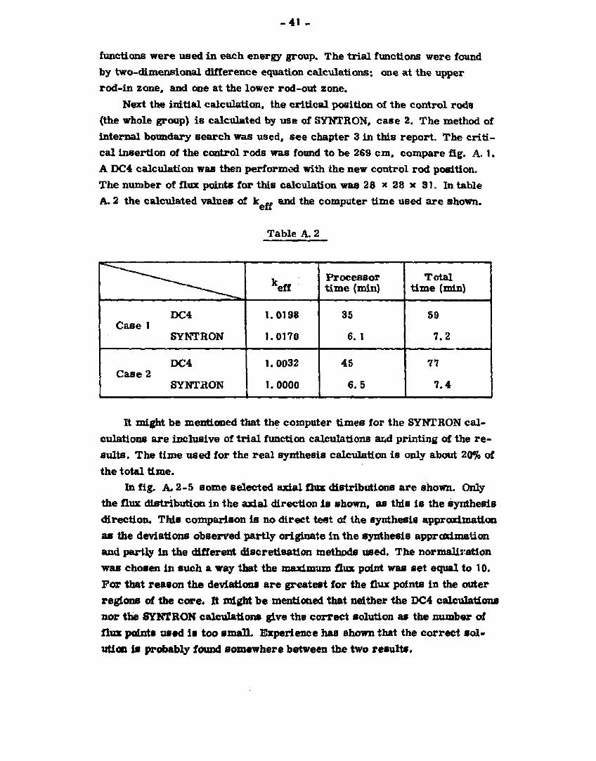
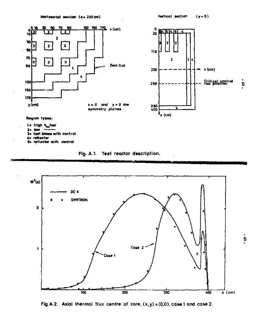
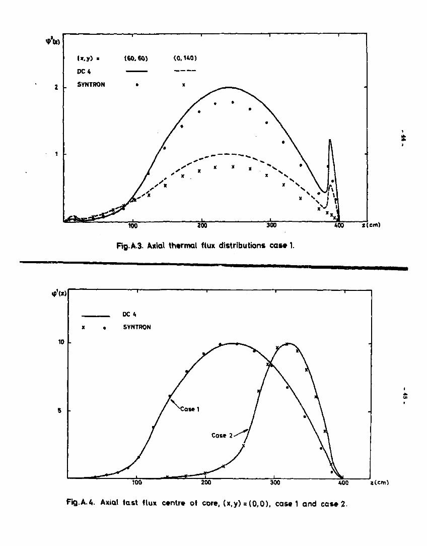
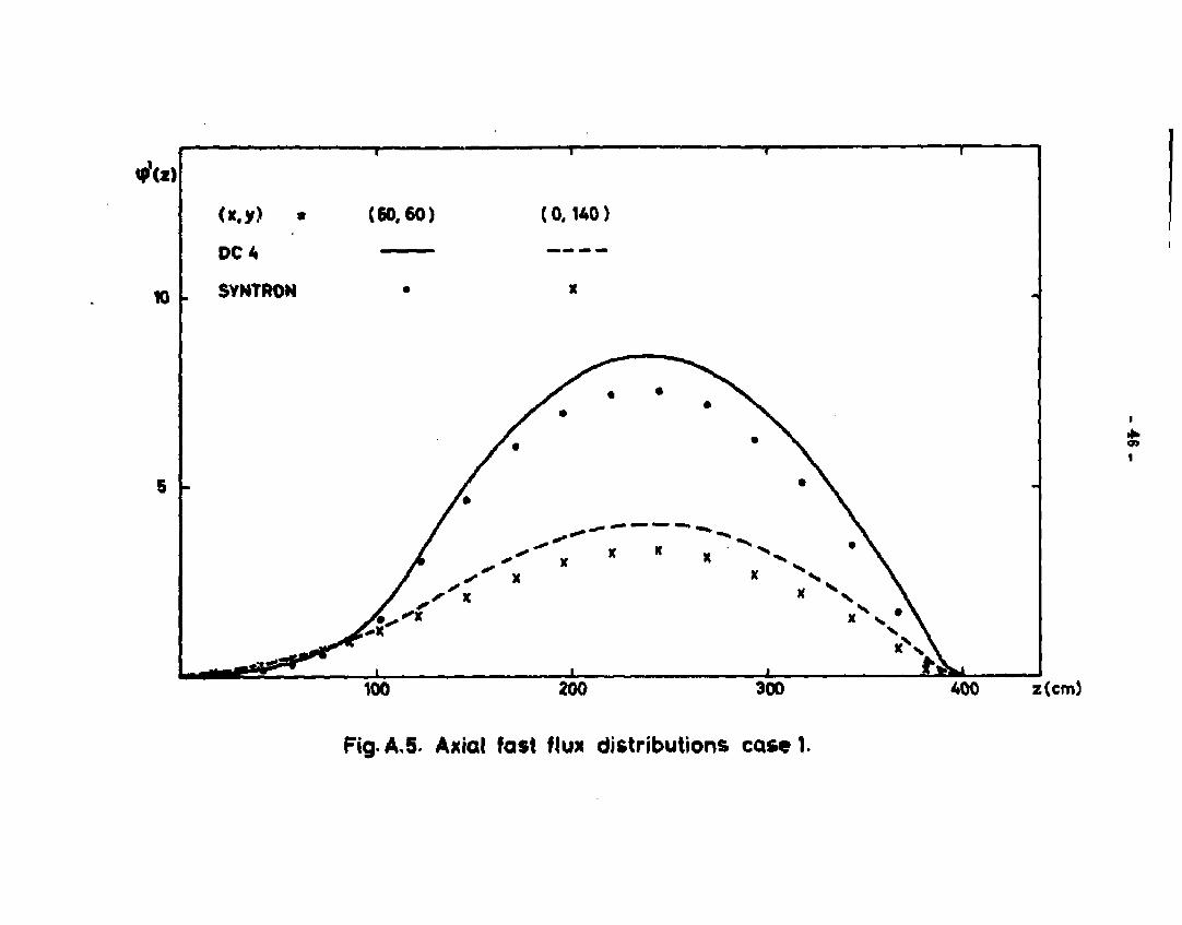
In fig. A, 2-5 some selected axial flux distributions are shown. Only the flux distribution in the axial direction is shown, as this is the synthesis direction. This comparison is no direct test of the synthesis approximation as the deviations observed partly originate in the synthesis approximation and partly in the different discretisation methods used. The normalisation was chosen in such a way that the maximum flux point was set equal to 10. For that reason the deviations are greatest for the flux points in the outer regions of the core. It might be mentioned that neither the DC4 calculations nor the SYNTRON calculations give the correct solution as the number of flux points used is too small Experience has shown that the correct sol­ution is probably found somewhere between the two results.

Herizontol »»etion d « 200 cm) Vertical. Mctiort (y = 0)

ttf W M—T-T-?" "(a")

Z*ro flu«

yicm)

Region types:

1« high H^fwl 2« low — «-— 9* tu*> boxe« with control «• nttttcter 5« i*ft#ctor with control

x • 0 and y * 0 ore »ymmvlry plan**

0 20

110

200

269

380 400

6.

3

L £ S

'« (cm)

• * K ( cm)

Critical fiftntrol Sd - rod position

Fig. A.I. Test reactor description.

•MHMMNUHHIMaaHBIbjHMMBHBHHi

z (cm)

Fig.A.2. Axial thermal flux centre of core, (x.y) = (0,0), easel and case2.

cm)

Fig.A3. Axial thermal flux distributions case 1.

100 200 300 400 *(cm)

Ftg.A.4. Axial fast flux centre of core, (x,y) = (0,0), easel and case 2.

tf<*>

10

5

<*.y) «

DC 4

SYNTRON

-

1 — 1 1 • — — t "

(60,60) (0, UO)

*

/ • \

/ „' X * V \

100 200 300 400 z(cm)

Fig. A,5. Axial fast flux distributions case 1.

-47 -

REFERENCES

1) S. Glasstone and M. C. Edlund, The Elements of Nuclear Reactor Theory, (D. van Nostrand Co., Princeton, N .J . , 1963) 416 pp.

2) J. H. Ferziger and P .F . Zweifel. The Theory of Neutron Slowing

Down in Nuclear Reactors, (Pergamon Press , Oxford, 1966) 310 pp.

3) K.E. Lindstrøm Jensen, Development and Verification of Nuclear Calculation Methods for Light-Water Reactors. Rise Report No. 235 (1970) 161 pp.

4) R. S. Varga, Matrix Iterative Analysis (Prentice-Hall, Engle-wood Cliffs, N .J . , 1962) 322 pp. '

5) H. Larsen, SYNTRON, A Three-Dimensional Flux Synthesis Pro­gramme« Rise-M-1346 (1971) 33 pp.

6) G.K. Kristiansen, Rise, Denmark, personal communication, 1972.

7} G.K. Kristiansen, DC4 Today, Risø, Denmc-k, RF-memo No. 183. To be published. Internal Report.

8) G.K. Kristiansen, H. Larsen,and B, Micheelsen, The 3D Benchmark Problem, Risø, Denmark. RF-memo No. 187 (1972). Internal Report.

9) D. L. Delp et aL , Flare, A Three-Dimensional Boiling Water Reactor Simulator, GEAP-4598 (1964) 95 pp.

10) L. Goldstein et aL» Calculation of Fuel-Cycle Burnup and Power Distribution of DRESDEN-I Reactor with the TRILUX Fuel Manage­ment Program. Trans. Amer. Nucl. Sec. H> (1967) 300.

11) A. F. Henry, Refinements in Accuracy of Coarse Mesh Finite Differ­ence Solution of the Group Diffusion Equations, IAEA Seminar on Numerical Reactor Calculations, Vienna, 17-21 January 1972,

12) C M . Rang, Finite Element Methods for Space-Time Reactor Anal­

ysis* MIT-3903-5 (1971) 192 pp.

13) S. Børresen, A flUmiUfied, Coarse-Mesh, Three-Dimensional Dif­

fusion Scheme for Calculating the Gross Power Distribution in a

Boiling Water Reactor. NucL Sci. Eng. 44 (1971) 37-43.

14) J. E. Meyer* Synthesis of Three-Dimensional Power Shapes - a Flux -

Weighting Synthesis Technique. Inj Proceedings of the 2nd United

Nations International Conference on the Peaceful Uses of Atomic En-

- 4 8 -

ergy, Geneva, 1-13 September 1958, Y\. (United Nations, Geneva, 1958) 519-522.

15) E. L. Wachspress et a l . , Multichannel Flux Synthesis. Nucl. Sci.

Eng. ^2 (1962) 381-389.

16) S. Kaplan, Some New Methods of Flu^ Synthesis. Nucl. Sci. Eng. Jj*

(1962) 22-31.

17) S. Kaplan et aL , Equations and Programs for Solutions of the Neutron

Group Diffusion Equations by Synthesis Approximations. WAPD-TM-

377 (1963) 67 pp.

18) G. Buckel, Approximation der stationaren, dreidimensionalen Mehr-

gruppen-Neutronen-Diffusionsgleichung durch ein Synthese\ erfahren

mit dem Karlsruher Synthese-Programm KASY, KFK 1349 (1971)

87 pp.

19) J. B. Yasinsky and S. Kaplan, Synthesis of Three-Dimensional Flux

Shapes Using Discontinuous Sets of Trial Functions. Nucl. Sci. Eng.

28 (1967) 426-437.

20) C. GrSgg, TRESYN - A Program for Calculation of the 3-Dimensional Neutron Flux Using Synthesis Techniques. AE-RD-20 (1970). AB Atom­energi, Sweden.

21) H. Larsen, Experience with Flux Synthesis for Burn-up Calculations on Light Water Reactors. IAEA Seminar on Numerical Reactor Calcu­lations, Vienna, 17-21 January 1972. 17 pp.

22) T. B. Fowler and M. L. Tobias, WMrlaway - A Three-Dimensional,

Two-Group Neutron Diffusion Code for the IBM 7090 Computer

ORNL-3150 (1961) 30 pp.

23) A. M. H. Larsen, H. Larsen and T. Petersen, Calculations on a

Boiling Water Reactor as a Test of the Risø Reactor Code Complex.

Risø Report No. 268 (1972) 102 pp.

24) S. Weber; Xenon-inducerede rumlige effekt oscillationer. Master

Thesis, Danish Atomic Energy Commission, Risø (in Danish 1871)

63 pp. Not published.

25) T. Petersen, Risø, Denmark, personal communication, 1972. j