Embed Size (px)
Citation preview
UNCORRECTED PROOF
Neural maps in remote sensing image analysis
Thomas Villmanna,*, Erzsebet Merenyib, Barbara Hammerc
aKlinik fur Psychotherapie, Universitat Leipzig, Karl-Tauchnitz-Str. 25, 04107 Leipzig, GermanybDepartment of Electrical and Computer Engineering, Rice University, 6100 Main Street, MS 380 Houston, TX, USA
cDepartment of Mathematics/Computer Science, University of Osnabruck, Albrechtstraße 28, 49069 Osnabruck, Germany
Abstract
We study the application of self-organizing maps (SOMs) for the analyses of remote sensing spectral images. Advanced airborne and
satellite-based imaging spectrometers produce very high-dimensional spectral signatures that provide key information to many scientific
investigations about the surface and atmosphere of Earth and other planets. These new, sophisticated data demand new and advanced
approaches to cluster detection, visualization, and supervised classification. In this article we concentrate on the issue of faithful topological
mapping in order to avoid false interpretations of cluster maps created by an SOM. We describe several new extensions of the standard SOM,
developed in the past few years: the growing SOM, magnification control, and generalized relevance learning vector quantization, and
demonstrate their effect on both low-dimensional traditional multi-spectral imagery and ,200-dimensional hyperspectral imagery.
q 2003 Published by Elsevier Science Ltd.
Keywords: Self-organizing map; Remote sensing; Generalized relevance learning vector quantization
1. Introduction
In geophysics, geology, astronomy, as well as in many
environmental applications air- and satellite-borne remote
sensing spectral imaging has become one of the most
advanced tools for collecting vital information about the
surface of Earth and other planets. Spectral images consist
of an array of multi-dimensional vectors each of which is
assigned to a particular spatial area, reflecting the response
of a spectral sensor for that area at various wavelengths
(Fig. 1). Classification of intricate, high-dimensional
spectral signatures has turned out to be far from trivial.
Discrimination among many surface cover classes, dis-
covery of spatially small, interesting spectral species proved
to be an insurmountable challenge to many traditional
clustering and classification methods. By customary
measures (such as, for example, principal component
analysis (PCA) the intrinsic spectral dimensionality of
hyperspectral images appears to be surprisingly low, 5–10
at most. Yet dimensionality reduction to such low numbers
has not been successful in terms of preservation of
important class distinctions. The spectral bands, many of
which are highly correlated, may lie on a low-dimensional
but non-linear manifold, which is a scenario that eludes
many classical approaches. In addition, these data comprise
enormous volumes and are frequently noisy. This motivates
research into advanced and novel approaches for remote
sensing image analysis and, in particular, neural networks
(Merenyi, 1999). Generally, artificial neural networks
attempt to replicate the computational power of biological
neural networks, with the following important (incomplete
list of) features:
† adaptivity—the ability to change the internal represen-
tation (connection weights, network structure) if new
data or information are available;
† robustness—handling of missing, noisy ore otherwise
confused data;
† power/speed—handling of large data volumes in accep-
table time due to inherent parallelism;
† non-linearity—the ability to represent non-linear func-
tions or mappings.
Exactly these properties make the application of neural
networks interesting in remote sensing image analysis. In
the present contribution, we will concentrate on a special
neural network type, neural maps. Neural maps constitute an
important neural network paradigm. In brains, neural maps
occur in all sensory modalities as well as in motor areas. In
technical contexts, neural maps are utilized in the fashion of
neighborhood preserving vector quantizers. In both cases
0893-6080/03/$ - see front matter q 2003 Published by Elsevier Science Ltd.
doi:10.1016/S0893-6080(03)00021-2
Neural Networks xx (0000) 1–15
www.elsevier.com/locate/neunet
* Corresponding author. Tel.: þ49-341-9718868; fax: þ49-341-
2131257.
E-mail address: [email protected] (T. Villmann).
NN 1720—1/3/2003—13:50—SUREKHA—64643— MODEL 5
ARTICLE IN PRESS
1
2
3
4
5
6
7
8
9
10
11
12
13
14
15
16
17
18
19
20
21
22
23
24
25
26
27
28
29
30
31
32
33
34
35
36
37
38
39
40
41
42
43
44
45
46
47
48
49
50
51
52
53
54
55
56
57
58
59
60
61
62
63
64
65
66
67
68
69
70
71
72
73
74
75
76
77
78
79
80
81
82
83
84
85
86
87
88
89
90
91
92
93
94
95
96
97
98
99
100
101
102
103
104
105
106
107
108
109
110
111
112

UNCORRECTED PROOFthese networks project data from some possibly high-
dimensional input space onto a position in some output
space. In the area of spectral image analysis we apply neural
maps for clustering, data dimensionality reduction, learning
of relevant data dimensions and visualization. For this
purpose we highlight several useful extensions of the basic
neural map approaches.
This paper is structured as follows. In Section 2 we
briefly introduce the problems in remote sensing spectral
image analysis. In Section 3 we give the basics of neural
maps and vector quantization together with a short review of
new extensions: structure adaptation and magnification
control (Section 3.2), and learning of proper metrics or
relevance learning (Section 3.3). In Section 4 we present
applications of the reviewed methods to multi-spectral
LANDSAT TM imagery as well as very high-dimensional
hyperspectral AVIRIS imagery.
2. Remote sensing spectral imaging
As mentioned earlier air- and satellite-borne remote
sensing spectral images consist of an array of multi-
dimensional vectors assigned to particular spatial regions
(pixel locations) reflecting the response of a spectral sensor
at various wavelengths. These vectors are called spectra. A
spectrum is a characteristic pattern that provides a clue to
the surface material within the respective surface element.
The utilization of these spectra includes areas such as
mineral exploration, land use, forestry, ecosystem manage-
ment, assessment of natural hazards, water resources,
environmental contamination, biomass and productivity;
and many other activities of economic significance, as well
as prime scientific pursuits such as looking for possible
sources of past or present life on other planets. The number
of applications has dramatically increased in the past 10
years with the advent of imaging spectrometers such as
AVIRIS of NASA/JPL, that greatly surpass the traditional
multi-spectral sensors (e.g. LANDSAT thematic mapper
(TM).
Imaging spectrometers can resolve the known, unique,
discriminating spectral features of minerals, soils, rocks,
and vegetation. While a multi-spectral sensor samples a
given wavelength window (typically the 0.4 2 2.5 mm
range in the case of visible and near-infrared imaging)
with several broad bandpasses, leaving large gaps
between the bands, imaging spectrometers sample a
spectral window contiguously with very narrow,
10 2 20 nm badpasses (Fig. 1) (Richards & Jia, 1999).
Hyperspectral technology is in great demand because
direct identification of surface compounds is possible
Fig. 1. Comparison of the spectral resolution of the AVIRIS hyperspectral
imager and the LANDSAT TM imager in the visible and near-infrared
spectral range. AVIRIS represents a quasi-continuous spectral sampling
whereas LANDSAT TM has coarse spectral resolution with large gaps
between the band passes. Additionally, spectral reflectance charateristics of
common earth surface materials is shown: 1, water; 2, vegetation; 3, soil
(from Richards and Jia (1999)).
Fig. 2. Left: The concept of hyperspectral imaging. Figure from Campbell (1996). Right: The spectral signature of the mineral alunite as seen through the six
broad bands of Landsat TM, as seen by the moderate spectral resolution sensor MODIS (20 bands in this region), and as measured in laboratory. Figure from
Clark (1999). Hyperspectral sensors such as AVIRIS of NASA/JPL (Green, 1996) produce spectral details comparable to laboratory measurements.
NN 1720—1/3/2003—13:50—SUREKHA—64643— MODEL 5
T. Villmann et al. / Neural Networks xx (0000) 1–152
ARTICLE IN PRESS
113
114
115
116
117
118
119
120
121
122
123
124
125
126
127
128
129
130
131
132
133
134
135
136
137
138
139
140
141
142
143
144
145
146
147
148
149
150
151
152
153
154
155
156
157
158
159
160
161
162
163
164
165
166
167
168
169
170
171
172
173
174
175
176
177
178
179
180
181
182
183
184
185
186
187
188
189
190
191
192
193
194
195
196
197
198
199
200
201
202
203
204
205
206
207
208
209
210
211
212
213
214
215
216
217
218
219
220
221
222
223
224

UNCORRECTED PROOF
without prior field work, for materials with
known spectral signatures. Depending on the wavelength
resolution and the width of the wavelength window used
by a particular sensor, the dimensionality of the spectra
can be as low as 5–6 (such as in LANDSAT TM), or as
high as several hundred for hyperspectral imagers
(Green, 1996).
Spectral images can formally be described as a matrix
S ¼ vðx;yÞ; where vðx;yÞ [ RDV is the vector of spectral
information associated with pixel location ðx; yÞ: The
elements vðx;yÞi ; i ¼ 1…DV of spectrum vðx;yÞ reflect the
responses of a spectral sensor at a suite of wavelengths
(Fig. 2; Campbell, 1996; Clark, 1999). The spectrum is a
characteristic fingerprint pattern that identifies the surface
material within the area defined by pixel ðx; yÞ: The
individual two-dimensional image Si ¼ vðx;yÞi at wave-
length i is called the ith image band. The data space V
spanned by visible–near infrared reflectance spectra is
½0 2 noise;U þ noise�DV # RDV where U . 0 represents
an upper limit of the measured scaled reflectivity and
noise is the maximum value of noise across all spectral
channels and image pixels. The data density PðVÞ may
vary strongly within this space. Sections of the data space
can be very densely populated while other parts may be
extremely sparse, depending on the materials in the scene
and on the spectral bandpasses of the sensor. According to
this model traditional multi-spectral imagery has a low
DV value while DV can be several hundred for
hyperspectral images. The latter case is of particular
interest because the great spectral detail, complexity, and
very large data volume pose new challenges in clustering,
cluster visualization, and classification of images with
such high spectral dimensionality (Merenyi, 1998).
In addition to dimensionality and volume, other factors,
specific to remote sensing, can make the analyses of
hyperspectral images even harder. For example, given the
richness of data, the goal is to separate many cover classes,
however, surface materials that are significantly different for
an application may be distinguished by very subtle
differences in their spectral patterns. The pixels can be
mixed, which means that several different materials may
contribute to the spectral signature associated with one
pixel. Training data may be scarce for some classes, and
classes may be represented very unevenly. All these
difficulties motivate research into advanced and novel
approaches (Merenyi, 1999).
Noise is far less problematic than the intricacy of the
spectral patterns, because of the high signal-to-noise ratios
(500–1500) that present-day hyperspectral imagers provide.
For this discussion, we will omit noise issues, and additional
effects such as atmospheric distortions, illumination geo-
metry and albedo variations in the scene, because these can
be addressed through well-established procedures prior to
clustering or classification.
3. Neural maps and vector quantization
3.1. Basic concepts and notations
Neural maps as tools for (unsupervised) topographic
vector quantization algorithms map data vectors v sampled
from a data manifold V # RDV onto a set A of neurons r
CV!A : V!A: ð3:1Þ
Associated with each neuron is a pointer (weight vector)
wr [ RDV specifying the configuration of the neural map
W ¼ {wr}r[A: The task of vector quantization is realized
by the map C as a winner-take-all rule, i.e. a stimulus
vector v [ V is mapped onto that neuron s [ A the
pointer ws of which is closest to the presented stimulus
vector v;
CV!A : v 7! sðvÞ ¼ argminr[A
dðv;wrÞ: ð3:2Þ
where dðv;wrÞ is the Euclidean distance. The neuron s is
referred to as the winner or best-matching unit. The
reverse mapping is defined as CA!V : r 7! wr: These two
mappings together determine the neural map
M ¼ ðCV!A;CA!VÞ; ð3:3Þ
realized by the network. The subset of the input space
Vr ¼ {v [ V : r ¼ CV!AðvÞ}; ð3:4Þ
which is mapped to a particular neuron r according to Eq.
(3.2), forms the (masked) V receptive field of that neuron.
If the intersection of two masked receptive fields Vr; Vr0
is non-vanishing we call Vr and Vr0 neighbored. The
neighborhood relations form a corresponding graph
structure GV in A : two neurons are connected in GV
if and only if their masked receptive fields are neighbored.
The graph GV is called the induced Delaunay-graph (See,
for example, Martinetz and Schulten (1994) for detailed
definitions). Due to the bijective relation between neurons
and weight vectors, GV also represents the Delaunay
graph of the weights (Martinetz & Schulten, 1994).
In the most widely used neural map algorithm, the self-
organizing map (SOM) (Kohonen, 1995), the neurons are
arranged a priori on a fixed grid A.1 Other algorithms such
as the topology representing network (TRN), which is based
on the neural gas algorithm (NG) (Martinetz, Berkovich, &
Schulten, 1993), do not specify the topological relations
among neurons, but construct a neighborhood structure in
the output space during learning (Martinetz & Schulten,
1994).
In any of these algorithms the pointers are adapted
such that the input data are matched appropriately. For
this purpose a random sequence of data points v [ Vfrom the stimuli distribution PðvÞ is presented to the
1 Usually the grid A is chosen as a dA-dimensional hypercube and then
one has i ¼ ði1;…; idAÞ: Yet, other ordered arrangements are also
admissible.
NN 1720—1/3/2003—13:52—SUREKHA—64643— MODEL 5
T. Villmann et al. / Neural Networks xx (0000) 1–15 3
ARTICLE IN PRESS
225
226
227
228
229
230
231
232
233
234
235
236
237
238
239
240
241
242
243
244
245
246
247
248
249
250
251
252
253
254
255
256
257
258
259
260
261
262
263
264
265
266
267
268
269
270
271
272
273
274
275
276
277
278
279
280
281
282
283
284
285
286
287
288
289
290
291
292
293
294
295
296
297
298
299
300
301
302
303
304
305
306
307
308
309
310
311
312
313
314
315
316
317
318
319
320
321
322
323
324
325
326
327
328
329
330
331
332
333
334
335
336

UNCORRECTED PROOF
map, the winning neuron s is determined according to
Eq. (3.2), and the pointer ws is shifted toward v:
Interactions among the neurons are included via a
neighborhood function determining to what extent the
units that are close to the winner in the output space
participate in the learning step
Dwr ¼ ehlðr; s; vÞðv 2 wrÞ: ð3:5Þ
hlðr; s; vÞ is usually chosen to be of Gaussian shape
hlðr; s; vÞ ¼ exp 2ðdAðr; sðvÞÞÞ2
l
!; ð3:6Þ
where dAðr; sðvÞÞ is a distance measure on the set A.
We emphasize that hlðr; s; vÞ implicitly depends on the
whole set W of weight vectors via the winner
determination of s according to Eq. (3.2). In SOMs it
is evaluated in the output space A : dSOMA ðr; sðvÞÞ ¼ kr 2
sðvÞkA whereas for the NG we have dNGA ðr; sðvÞÞ ¼ krðv;
WÞ: krðv;WÞ gives the number of pointers wr0 for which
the relation dðv;wr0 Þ # dðv;wrÞ is valid (Martinetz et al.,
1993), i.e. dNGA is evaluated in the input space (Here, dð; Þ
is the Euclidean distance.). In the SOM usually l ¼ 2s2
is used.
The particular definitions of the distance measures in
the two models cause further differences. In Martinetz
et al. (1993) the convergence rate of the neural gas
network was shown to be faster than that of the SOM.
Furthermore, it was proven that the adaptation rule for
the weight vectors follows, on average, a potential
dynamic. In contrast, a global energy function does not
exist in the SOM algorithm (Erwin, Obermayer, &
Schulten, 1992).
One important extension of the basic concepts of neural
maps concerns the so-called magnification. The standard
SOM distributes the pointers according to the input
distribution
PðWÞ , PðVÞa; ð3:7Þ
with the magnification factor aSOM ¼ 23
(Ritter &
Schulten, 1986; Kohonen, 1999).2,3 For the NG one
finds, by analytical considerations, that for small l the
magnification factor aNG ¼ d=ðd þ 2Þ which only depends
on the dimensionality of the input space embedded in
RDV ; i.e. the result is valid for all dimensions (Martinetz
et al., 1993).
Topology preservation or topographic mapping in
neural maps is defined as the preservation of the
continuity of the mapping from the input space onto
the output space, more precisely it is equivalent to the
continuity of M between the topological spaces with
properly chosen metric in both A and V: For lack of
space we refer to Villmann, Der, and Herrmann (1997) for
detailed considerations. For the TRN the metric in A is
defined according to the given data structure whereas in
case of the SOM violations of topology preservation may
occur if the structure of the output space does not match
the topological structure of V In SOMs the topology
preserving property can be used for immediate evaluations
of the resulting map, for instance by interpretation as a
color space, as demonstrated in Section 4.2.2. Topology
preservation also allows the applications of interpolating
schemes such as the parametrized SOM (PSOM) (Ritter,
1993) or interpolating SOM (I-SOM) (Goppert &
Rosenstiel, 1997). A higher degree of topology preser-
vation, in general, improves the accuracy of the map
(Bauer & Pawelzik, 1992).
As pointed out in Villmann et al. (1997) violations of
topographic mapping in SOMs can result in false
interpretations. Several approaches were developed to
judge the degree of topology preservation for a given
map. Here we briefly describe a variant ~P of the well
known topographic product P (Bauer & Pawelzik, 1992).
Instead of the Euclidean distances between the
weight vectors, ~P uses the respective distances dGVðwr;
wr0 Þ of minimal path lengths in the induced Delaunay-
graph GV of the wr: During the computation of ~P for
each node r the sequences nAj ðrÞ of jth neighbors of r in
A; and nVj ðrÞ describing the jth neighbor of wr in V;
have to be determined. These sequences and further
averaging over neighborhood orders j and nodes r finally
lead to
~P ¼1
NðN 2 1Þ
Xr
XN21
j¼1
1
2jlogðQÞ; ð3:8Þ
with
Q ¼ Pjl¼1
dGV ðwr;wnAlðrÞÞ
dGV ðwr;wnVlðrÞÞ
dAðr; nAl ðrÞÞ
dAðr; nVl ðrÞÞ
; ð3:9Þ
and dAðr; r0Þ is the distance between the neuron positions
r and r0 in the lattice A: ~P can take on positive or
negative values with similar meaning as for the original
topographic product P : if ~P , 0 holds the output space
is too low-dimensional, and for ~P . 0 the output space is
too high-dimensional. In both cases neighborhood
relations are violated. Only for ~P < 0 does the output
space approximately match the topology of the input
data. The present variant ~P overcomes the problem of
strongly curved maps which may be judged neighbor-
hood violating by the original P even though the shape
of the map might be perfectly justified (Villmann et al.,
1997).
2 This result is valid for the one-dimensional case and higher-dimensional
ones which separate.3 The notation ‘magnification factor’ is, strictly speaking, not correct.
Some times it is called (mathematically exact) magnification exponent.
However, the notation ‘magnification factor’ is commonly used (van Hulle,
2000). Therefore we use this notation here.
NN 1720—1/3/2003—13:52—SUREKHA—64643— MODEL 5
T. Villmann et al. / Neural Networks xx (0000) 1–154
ARTICLE IN PRESS
337
338
339
340
341
342
343
344
345
346
347
348
349
350
351
352
353
354
355
356
357
358
359
360
361
362
363
364
365
366
367
368
369
370
371
372
373
374
375
376
377
378
379
380
381
382
383
384
385
386
387
388
389
390
391
392
393
394
395
396
397
398
399
400
401
402
403
404
405
406
407
408
409
410
411
412
413
414
415
416
417
418
419
420
421
422
423
424
425
426
427
428
429
430
431
432
433
434
435
436
437
438
439
440
441
442
443
444
445
446
447
448

UNCORRECTED PROOF
3.2. Magnification control and structure adaptation
3.2.1. Magnification control
The first approach to influence the magnification of a
vector quantizer, proposed in DeSieno (1988), is called
the mechanism of conscience yielding approximately the
same winning probability for each neuron. Hence, the
approach yields density matching between input and
output space which corresponds to a magnification factor
of 1. Bauer, Der, and Herrmann (1996) suggested a more
general scheme for the SOM to achieve an arbitrary
magnification. They introduced a local learning parameter
e s for each neuron r with ke sl/PðwrÞm in Eq. (3.5),
where m is an additional control parameter. Eq. (3.5) now
reads as
Dwr ¼ e shlðr; s; vÞðv 2 wrÞ: ð3:10Þ
Note that the learning factor e s of the winning neuron s is
applied to all updates. This local learning leads to a
similar relation as in Eq. (3.7)
PðWÞ , PðVÞa0
; ð3:11Þ
with a0 ¼ aðm þ 1Þ and allows a magnification control
through the choice of m: In particular, one can achieve a
resolution of a0 ¼ 1; which maximizes mutual information
(Linsker, 1989; Villmann & Herrmann, 1998). Application
of this approach to the derivation of the dynamic of TRN
yields exactly the same result (Villmann, 2000).
3.2.2. Structure adaptation
For both neural map types, the SOM and the TRN,
growing variants for structure adaptation are known.
In the growing SOM (GSOM) approach the output Ais a hypercube in which both the dimension and the
respective length ratios are adapted during the learning
procedure in addition to the weight vector learning, i.e.
the overall dimensionality and the dimensions along the
individual directions change in the hypercube. The GSOM
starts from an initial 2-neuron chain, learns according the
regular SOM-algorithm, adds neurons to the output space
according to a certain criterion to be described later,
learns again, adds again, etc. until a prespecified
maximum number Nmax of neurons is distributed. During
this procedure, the output space topology remains of the
form n1 £ n2 £ · · ·; with nj ¼ 1 for j . DA; where DA is
the current dimensionality of A:4 From there it can grow
either by adding nodes in one of the directions which are
already spanned by the output space or by initialising a
new dimension. This decision is made on the basis of the
receptive fields Vr: When reconstructing v [ V from
neuron r; an error u ¼ v 2 wr remains decomposed along
the different directions, which results from projecting back
the output grid A into the input space V
u ¼ v 2 wr ¼XDA
i¼1
aiðvÞwrþei
2 wr2ei
kwrþei2 wr2ei
kþ v0
: ð3:12Þ
Here, ei denotes the unit vector in direction i of A; wrþei
and wr2eiare the weight vectors of the neighbors of the
neuron r in the ith direction of the lattice A:5 Considering
a receptive field Vr and determining the first principle
component vPCA of Vr allows a further decomposition of
v0
: Projection of v0
onto the direction of vPCA then yields
aDAþ1ðvÞ;
v0
¼ aDAþ1ðvÞvPCA
kvPCAkþ v
00
: ð3:13Þ
The criterion for the growing now is to add nodes in that
direction which has, on average, the largest of the
expected (normalized) error amplitudes ~ai
~ai ¼
ffiffiffiffiffiffiffiffiffini
ni þ 1
r Xv[Vr
laiðvÞlffiffiffiffiffiffiffiffiffiffiffiffiffiffiffiPDAþ1j¼1 a2
j ðvÞq ;
i ¼ 1;…;DA þ 1:
ð3:14Þ
After each growth step, a new learning phase has to take
place, in order to readjust the map. For a detailed study of
the algorithm we refer to Bauer and Villmann (1997).
The growing TRN adapts the number of neurons in TRN
whereby the structure between them is re-arranged accord-
ing to the TRN definition (Fritzke, 1995). Hence, it is
capable of representing the data space in a topologically
faithful manner with increasing accuracy and it also realizes
a structure adaptation.
3.3. Relevance learning
As mentioned earlier neural maps are unsupervised
learning algorithms. In case of labeled data one can apply
supervised classification schemes for vector quantization
(VQ). Assuming that the data are labeled, an automatic
clustering can be learned via attaching maps to the SOM or
adding a supervised component to VQ to achieve learning
vector quantization (LVQ) (Kohonen, Lappalainen, &
Saljarvi, 1997; Meyering & Ritter, 1992). Various modifi-
cations of LVQ exist which ensure faster convergence, a
better adaptation of the receptive fields to optimum
Bayesian decision, or an adaptation for complex data
4 Hence, the initial configuration is 2 £ 1 £ 1 £ · · ·;DA ¼ 1:
5 At the border of the output space grid, where not two, but just one
neighboring neuron is available, we use
wr 2 wr2ei
kwr 2 wr2eik
or
wrþei2 wr
kwr2ei2 wrk
to compute the backprojection of the output space direction ei into the input
space.
NN 1720—1/3/2003—13:52—SUREKHA—64643— MODEL 5
T. Villmann et al. / Neural Networks xx (0000) 1–15 5
ARTICLE IN PRESS
449
450
451
452
453
454
455
456
457
458
459
460
461
462
463
464
465
466
467
468
469
470
471
472
473
474
475
476
477
478
479
480
481
482
483
484
485
486
487
488
489
490
491
492
493
494
495
496
497
498
499
500
501
502
503
504
505
506
507
508
509
510
511
512
513
514
515
516
517
518
519
520
521
522
523
524
525
526
527
528
529
530
531
532
533
534
535
536
537
538
539
540
541
542
543
544
545
546
547
548
549
550
551
552
553
554
555
556
557
558
559
560

UNCORRECTED PROOF
structures, to mention just a few (Kohonen et al., 1997; Sato
& Yamada, 1995; Somervuo & Kohonen, 1999).
A common feature of unsupervised algorithms and LVQ
is the information provided by the distance structure in V;
which is determined by the chosen metric. Learning heavily
relies on this feature and therefore crucially depends on how
appropriate the chosen metric is for the respective learning
task. Several methods have been proposed which adapt the
metric during training (Kaski, 1998; Kaski & Sinkkonen,
1999; Pregenzer, Pfurtscheller, & Flotzinger, 1996).
Here we focus on metric adaptation for LVQ since the
LVQ combines the elegance of simple and intuitive updates
in unsupervised algorithms with the accuracy of supervised
methods. Let cv [ L be the label of input v; L a set of
labels (classes) with #L ¼ NL: LVQ uses a fixed number
of codebook vectors (weight vectors) for each class. Let
W ¼ {wr} be the set of all codebook vectors and cr be the
class label of wr: Furthermore, let Wc ¼ {wrlcr ¼ c} be the
subset of weights assigned to class c [ L:
The training algorithm adapts the codebook vectors
such that for each class c [ L; the corresponding
codebook vectors Wc represent the class as accurately as
possible. This means that the set of points in any given class
Vc ¼ {v [ Vlcv ¼ c}; and the union Uc ¼S
rlwr[WcVr of
receptive fields of the corresponding codebook vectors
should differ as little as possible. For a given data point v
with class label cv let mðvÞ denote some function which is
negative if v is classified correctly, i.e. it belongs to a
receptive field Vr with cr ¼ cv; and which is positive if v is
classified incorrectly, i.e. it belongs to a receptive field Vr
with cr – cv: Let f : R! R be some monotonically
increasing function. The general scheme of GLVQ aims to
minimize the cost function
Cost ¼X
v
f ðmðvÞÞ; ð3:15Þ
via stochastic gradient descent. Different choices of f and
mðvÞ yield LVQ or LVQ2.1 as introduced in Kohonen et al.
(1997), respectively, as shown in Sato and Yamada (1995).
Denote by d the squared Euclidean distance of v to the
nearest codebook vector. The choice of f as the sigmoidal
function and
mðvÞ ¼drþ
2 dr2
drþþ dr2
; ð3:16Þ
where drþis the squared Euclidean distance of the input
vector v to the nearest codebook vector labeled with crþ¼
cv; say wrþ; and dr2
is the squared Euclidean distance to the
best matching codebook vector but labeled with cr2– crþ
;
say wr2; yields a powerful and noise tolerant behavior since
it combines adaptation near the optimum Bayesian borders
similarly as in LVQ2.1, with prohibiting the possible
divergence of LVQ2.1 (as reported in Sato and Yamada
(1995)). We refer to this modification as the GLVQ. The
respective learning dynamic is obtained by differentiation of
the cost function (3.15) (Sato & Yamada, 1995)
Dwrþ¼ e
4f 0lmðvÞ·dr2
ðdrþþ dr2
Þ2ðv 2 wrþ
Þ and
Dwr2¼ 2e
4f 0lmðvÞ·drþ
ðdrþþ dr2
Þ2ðv 2 wr2
Þ:
ð3:17Þ
To result a metric adaptation we now introduce input
weights l ¼ ðl1;…;lDVÞ; li $ 0; klk ¼ 1 in order to allow
a different scaling of the input dimensions: substituting the
squared Euclidean metric by its scaled variant
dlðx; yÞ ¼XDV
i¼1
liðxi 2 yiÞ2; ð3:18Þ
the receptive field of codebook vector wr becomes
Vlr ¼ {v [ V : r ¼ Cl
V!AðvÞ}; ð3:19Þ
with
ClV!A : v 7! sðvÞ ¼ argmin
r[Adlðv;wrÞ; ð3:20Þ
as mapping rule. Replacing Vr by Vlr and d by dl in the cost
function ‘Cost’ in Eq. (3.15) yields a variable weighting of
the input dimensions and hence an adaptive metric. Now
Eq. (3.17) reads as
Dwrþ¼ e
4·f 0lmðvÞ·dlr2
ðdlrþ
þ dlr2Þ2Lðv 2 wrþ
Þ and
Dwr2¼ 2e
4·f 0lmðvÞ·dlrþ
ðdlrþ
þ dlr2Þ2Lðv 2 wr2
Þ;
ð3:21Þ
with L being the diagonal matrix with entries l1;…; lDV:
Appropriate weighting factors l can also be determined
automatically via a stochastic gradient descent. In this way
the GLVQ-learning rule (3.17) is augmented as follows
Dlk ¼2 e1·2·f 0lmðvÞdl
r2
ðdlrþ
þ dlr2Þ2ðv 2 wrþ
Þ2k
2dl
rþ
ðdlrþ
þ dlr2Þ2ðv 2 wr2
Þ2k
!; ð3:22Þ
with e1 [ ð0; 1Þ and k ¼ 1…DV; followed by normalization
to obtain klk ¼ 1: We term this generalization of the
relevance learning vector quantization (RLVQ) (Bojer,
Hammer, Schunk, & von Toschanowitz, 2001) and GLVQ
generalized relevance learning vector quantization
(GRLVQ) as introduced in Hammer and Villmann (2001a,
2002).
Obviously, the same idea could be applied to any
gradient dynamics. We could, for example, minimize a
different error function such as the Kullback–Leibler
divergence of the distribution which is to be learned and
the distribution which is implemented by the vector
quantizer. This approach is not limited to supervised
tasks. Unsupervised methods such as the NG (Martinetz
NN 1720—1/3/2003—13:52—SUREKHA—64643— MODEL 5
T. Villmann et al. / Neural Networks xx (0000) 1–156
ARTICLE IN PRESS
561
562
563
564
565
566
567
568
569
570
571
572
573
574
575
576
577
578
579
580
581
582
583
584
585
586
587
588
589
590
591
592
593
594
595
596
597
598
599
600
601
602
603
604
605
606
607
608
609
610
611
612
613
614
615
616
617
618
619
620
621
622
623
624
625
626
627
628
629
630
631
632
633
634
635
636
637
638
639
640
641
642
643
644
645
646
647
648
649
650
651
652
653
654
655
656
657
658
659
660
661
662
663
664
665
666
667
668
669
670
671
672

UNCORRECTED PROOF
et al., 1993), which obey a gradient dynamics, could be
improved by application of weighting factors in order to
obtain an adaptive metric. Furthermore, in unsupervised
topographic mapping models like the SOM or NG one
can try to learn the relevance of input dimensions subject to
the requirement of topology preservation (Hammer &
Villmann, 2001a,b).
3.4. Further approaches
Beside the above introduced methods further approaches
of neural inspired algorithms are well known. In this context
we have to refer to the family of fuzzy-clustering algorithms
as for instance Fuzzy-SOM (Bezdek & Pal, 1993; Graepel,
Burger, & Obermayer, 1998; Hasenjager, Ritter, &
Obermayer, 1999), Fuzzy-c-means (Bezdek, Pal, Hathaway,
& Karayiannis, 1995; Gath & Geva, 1989) or other (neural)
vector quantizers based on minimization of an energy
function (Bishop, Svensen, & Williams, 1998; Buhmann &
Kuhnel, 1993; Linsker, 1989). For an overview of respective
approaches we refer to Haykin (1994) (neural network
approaches), Duda and Hart, (1973), and Schurmann (1996)
(pattern classification).
4. Application in remote sensing image analysis
4.1. Low-dimensional data: LANDSAT TM multi-spectral
images
4.1.1. Image description
LANDSAT TM satellite-based sensors produce images
of the Earth in seven different spectral bands. The ground
resolution is 30 £ 30 m2 for bands 1–5 and band 7. Band 6
(thermal band) is often dropped from analyses because of
the lower spatial resolution. The LANDSAT TM bands
were strategically determined for optimal detection and
discrimination of vegetation, water, rock formations and
cultural features within the limits of broad band multi-
spectral imaging. The spectral information, associated with
each pixel of a LANDSAT scene is represented by a vector
v [ V # RDV with DV ¼ 6: The aim of any classification
algorithm is to subdivide this data space into subsets of data
points, with each subset corresponding to specific surface
covers such as forest, industrial region, etc. The feature
categories are specified by prototype data vectors (training
spectra).
In the present contribution we consider a LANDSAT TM
image from the Colorado area, USA.6 In addition we have a
manually generated label map (ground truth image) for the
assessment of classification accuracy. All pixels of the
Colorado image have associated ground truth labels,
categorized into 14 classes. The classes include several
regions of different vegetation and soil, and can be used for
supervised learning schemes like the GRLVQ (Table 1).
4.1.2. Analyses of LANDSAT TM imagery
A initial Grassberger–Procaccia analysis (Grassberger &
Procaccia, 1983) yields DGP < 3:1414 for the intrinsic
dimensionality (ID) of the Colorado image.
SOM analysis. The GSOM generates a 12 £ 7 £ 3 lattice
(Nmax ¼ 256) in agreement with the Grassberger–Procaccia
analysis (DGP < 3:1414), which corresponds to a ~P-value
of 0.0095 indicating good topology preservation (Fig. 3).
One way to visualize the GSOM clusters of LANDSAT
TM data is to use a SOM dimension DA ¼ 3 (Gross &
Seibert, 1993) and interpret the positions of the neurons r in
the lattice A as vectors cðrÞ ¼ ðr; g; bÞ in the RGB color
space, where r; g; b are the intensities of the colors red,
green and blue, respectively, computed as clðrÞ ¼ ½ðrl 2
1Þ=ðnl 2 1Þ�255; for l ¼ 1; 2; 3 (Gross & Seibert, 1993).
Table 1
Table of labels and classes occurring in the LANDSAT TM Colorado
image
Class label Ground cover type
a Scotch pine
b Douglas fir
c Pine/fir
d Mixed pine forest
e Supple/prickle pine
f Aspen/mixed pine forest
g Without vegetation
h Aspen
i Water
j Moist meadow
k Bush land
l Grass/pastureland
m Dry meadow
n Alpine vegetation
o Misclassification
Fig. 3. Left: the reference classification for the Landsat TM Colorado
image, provided by M. Augusteijn. Classed are keyed as shown on the color
wedge on the left, and the corresponding surface units are described in
Table 1. Right: cluster map of the Colorado image derived from all six
bands by the 12 £ 7 £ 3 GSOM-solution. Note that, due to the visualization
scheme, which uses a continuous scale of RGB colors described in the text,
this map does not show hard cluster boundaries. More similar colors
indicate more similar spectral classes.
6 Thanks to M. Augusteijn (Univerity of Colorado) for providing this
image.
NN 1720—1/3/2003—13:52—SUREKHA—64643— MODEL 5
T. Villmann et al. / Neural Networks xx (0000) 1–15 7
ARTICLE IN PRESS
673
674
675
676
677
678
679
680
681
682
683
684
685
686
687
688
689
690
691
692
693
694
695
696
697
698
699
700
701
702
703
704
705
706
707
708
709
710
711
712
713
714
715
716
717
718
719
720
721
722
723
724
725
726
727
728
729
730
731
732
733
734
735
736
737
738
739
740
741
742
743
744
745
746
747
748
749
750
751
752
753
754
755
756
757
758
759
760
761
762
763
764
765
766
767
768
769
770
771
772
773
774
775
776
777
778
779
780
781
782
783
784
UNCORRECTED PROOF
Such assignment of colors to winner neurons immediately
yields a pseudo-color cluster map of the original image for
visual interpretation. Since we are mapping the data clouds
from a six-dimensional input space onto a three-dimen-
sional color space dimensional conflicts may arise and the
visual interpretation may fail. However, in the case of
topologically faithful mapping this color representation,
prepared using all six LANDSAT TM image bands,
contains considerably more information than a customary
color composite combining three TM bands (frequently
bands 2, 3, and 3). (Gross & Seibert, 1993).
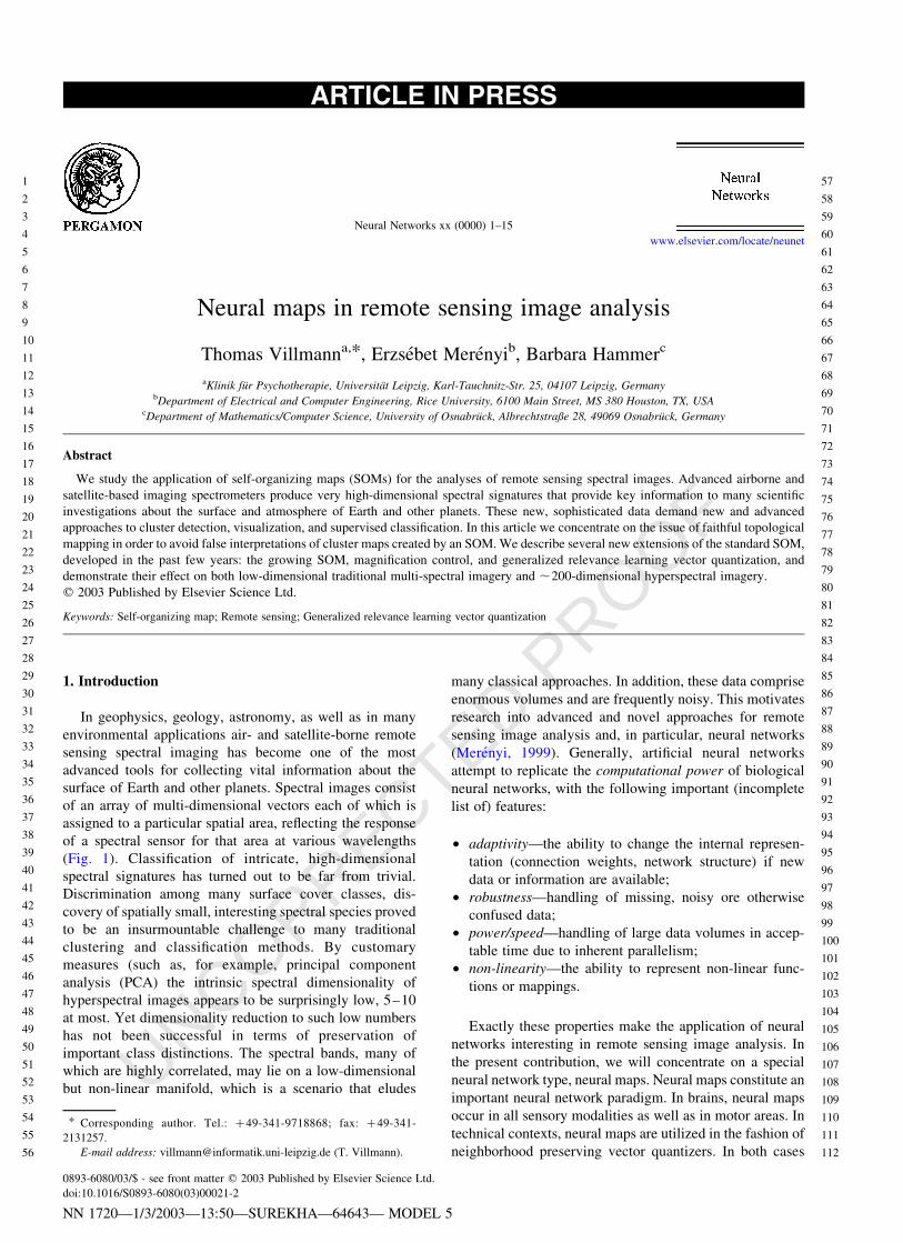
Application of GRLVQ. We trained the GRLVQ with 42
codebook vectors (three for each class) on 5% of the data set
until convergence. The algorithm converged in , 10 cycles
for e ¼ 0:1 and e1 ¼ 0:01: The GRLVQ produced a
classification accuracy of about 90% on the training set as
well as on the entire data set. The weighting factors resulting
from GRLVQ analysis provide a ranking of the data
dimensions
l5 ð0:1; 0:17; 0:27; 0:21; 0:26; 0:0Þ: ð4:1Þ
Clearly, dimension 6 is ranked as least important with
weighting factor close to 0. Dimension 1 is the second least
important followed by dimensions 2 and 4. Dimensions 3
and 5 are of similarly high importance according to this
ranking. If we prune dimensions 6, 1, and 2, an accuracy of
84% can still be achieved. Pruning dimension 4 brings the
classification accuracy down to 50%, which is a very
significant loss of information. This indicates that the
intrinsic data dimension may not be as low as 2. These
classification results are shown in Fig. 4 with misclassified
pixels colored black and classes keyed by the color wedge.
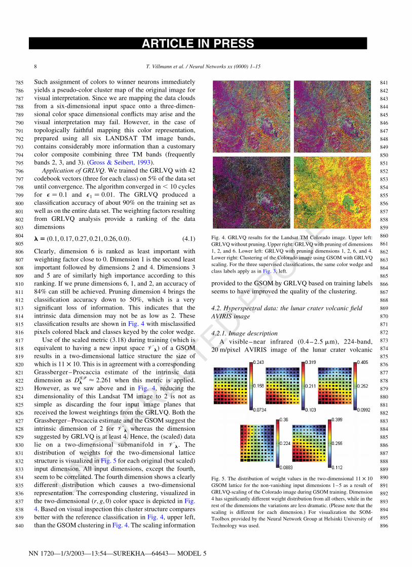
Use of the scaled metric (3.18) during training (which is
equivalent to having a new input space Vl) of a GSOM
results in a two-dimensional lattice structure the size of
which is 11 £ 10. This is in agreement with a corresponding
Grassberger–Procaccia estimate of the intrinsic data
dimension as DGPl < 2:261 when this metric is applied.
However, as we saw above and in Fig. 4, reducing the
dimensionality of this Landsat TM image to 2 is not as
simple as discarding the four input image planes that
received the lowest weightings from the GRLVQ. Both the
Grassberger–Procaccia estimate and the GSOM suggest the
intrinsic dimension of 2 for Vl whereas the dimension
suggested by GRLVQ is at least 4. Hence, the (scaled) data
lie on a two-dimensional submanifold in Vl: The
distribution of weights for the two-dimensional lattice
structure is visualized in Fig. 5 for each original (but scaled)
input dimension. All input dimensions, except the fourth,
seem to be correlated. The fourth dimension shows a clearly
different distribution which causes a two-dimensional
representation. The corresponding clustering, visualized in
the two-dimensional ðr; g; 0Þ color space is depicted in Fig.
4. Based on visual inspection this cluster structure compares
better with the reference classification in Fig. 4, upper left,
than the GSOM clustering in Fig. 4. The scaling information
provided to the GSOM by GRLVQ based on training labels
seems to have improved the quality of the clustering.
4.2. Hyperspectral data: the lunar crater volcanic field
AVIRIS image
4.2.1. Image description
A visible – near infrared (0.4 – 2.5 mm), 224-band,
20 m/pixel AVIRIS image of the lunar crater volcanic
Fig. 4. GRLVQ results for the Landsat TM Colorado image. Upper left:
GRLVQ without pruning. Upper right: GRLVQ with pruning of dimensions
1, 2, and 6. Lower left: GRLVQ with pruning dimensions 1, 2, 6, and 4.
Lower right: Clustering of the Colorado image using GSOM with GRLVQ
scaling. For the three supervised classifications, the same color wedge and
class labels apply as in Fig. 3, left.
Fig. 5. The distribution of weight values in the two-dimensional 11 £ 10
GSOM lattice for the non-vanishing input dimensions 1–5 as a result of
GRLVQ-scaling of the Colorado image during GSOM training. Dimension
4 has significantly different weight distribution from all others, while in the
rest of the dimensions the variations are less dramatic. (Please note that the
scaling is different for each dimension.) For visualization the SOM-
Toolbox provided by the Neural Network Group at Helsinki University of
Technology was used.
NN 1720—1/3/2003—13:54—SUREKHA—64643— MODEL 5
T. Villmann et al. / Neural Networks xx (0000) 1–158
ARTICLE IN PRESS
785
786
787
788
789
790
791
792
793
794
795
796
797
798
799
800
801
802
803
804
805
806
807
808
809
810
811
812
813
814
815
816
817
818
819
820
821
822
823
824
825
826
827
828
829
830
831
832
833
834
835
836
837
838
839
840
841
842
843
844
845
846
847
848
849
850
851
852
853
854
855
856
857
858
859
860
861
862
863
864
865
866
867
868
869
870
871
872
873
874
875
876
877
878
879
880
881
882
883
884
885
886
887
888
889
890
891
892
893
894
895
896

UNCORRECTED PROOF
field (LCVF), Nevada, USA, was analyzed in order to study
SOM performance for high-dimensional remote sensing
spectral imagery. (AVIRIS is the airborne visible-near
infrared imaging spectrometer, developed at NASA/Jet
Propulsion Laboratory. See http://makalu.jpl.nasa.gov for
details on this sensor and on imaging spectroscopy). The
LCVF is one of NASA’s remote sensing test sites, where
images are obtained regularly. A great amount of accumu-
lated ground truth from comprehensive field studies
(Arvidson et al., 1991) and research results from indepen-
dent earlier work such as Farrand (1991) provide a detailed
basis for the evaluation of the results presented here.
Fig. 6 shows a natural color composite of the LCVF with
labels marking the locations of 23 different surface cover
types of interest. This 10 £ 12 km2 area contains, among
other materials, volcanic cinder cones (class A, reddest
peaks) and weathered derivatives thereof such as ferric
oxide rich soils (L, M, W), basalt flows of various ages (F,
G, I), a dry lake divided into two halves of sandy (D) and
clayey composition (E); a small rhyolitic outcrop (B); and
some vegetation at the lower left corner (J), and along
washes (C). Alluvial material (H), dry (N,O,P,U) and wet
(Q,R,S,T) playa outwash with sediments of various clay
contents as well as other sediments (V) in depressions of the
mountain slopes, and basalt cobble stones strewn around the
playa (K) form a challenging series of spectral signatures for
pattern recognition (Merenyi, 1998). A long, NW–SE
trending scarp, straddled by the label G, borders the
vegetated area. Since this color composite only contains
information from three selected image bands (one red, one
green, and one blue), many of the cover type variations
remain undistinguished. They will become evident in the
cluster and class maps below.
After atmospheric correction and removal of excessively
noisy bands (saturated water bands and overlapping detector
channels), 194 image bands remained from the original 224.
These 194-dimensional spectra are the input patterns in the
following analyses.
The spectral dimensionality of hyperspectral images is
not well understood and it is an area of active research.
While many believe that hyperspectral images are highly
redundant because of band correlations, others maintain an
opposite view. Few investigations exist into the ID of
hyperspectral images. Linear methods such as PCA or
determination of mixture model endmembers (Adams,
Smith, & Gillespie, 1993; R.S. Inc, 1997) usually yield
3–8 ‘endmembers’. Optimally topology preserving maps, a
TRN approach (Bruske & Merenyi, 1999), finds the spectral
ID of the LCVF AVIRIS image to be between 3 and 7
whereas the Grassberger–Procaccia estimate (Grassberger
& Procaccia, 1983) for the same image is DGP < 3:06:
These surprisingly low numbers, that increase with
improved sensor performance (Green & Boardman, 2000),
result from using statistical thresholds for the determination
of what is ‘relevant’, regardless of application dependent
meaning of the data.
The number of relevant components increases dramati-
cally when specific goals are considered such as what cover
classes should be separated. With an associative neural
network, Pendock (1999) extracted 20 linear mixing
Fig. 6. The Lunar Crater Volcanic Field. RGB natural color composite from an AVIRIS, 1994 image. The full hyperspectral image comprises 224 image bands
over the 0.4–2.5 mm wavelength range, 512 £ 614 pixels, altogether 140 MB of data. Labels indicate 23 different cover types described in the text. The ground
resolution is 20 m/pixel.
NN 1720—1/3/2003—13:57—SUREKHA—64643— MODEL 5
T. Villmann et al. / Neural Networks xx (0000) 1–15 9
ARTICLE IN PRESS
897
898
899
900
901
902
903
904
905
906
907
908
909
910
911
912
913
914
915
916
917
918
919
920
921
922
923
924
925
926
927
928
929
930
931
932
933
934
935
936
937
938
939
940
941
942
943
944
945
946
947
948
949
950
951
952
953
954
955
956
957
958
959
960
961
962
963
964
965
966
967
968
969
970
971
972
973
974
975
976
977
978
979
980
981
982
983
984
985
986
987
988
989
990
991
992
993
994
995
996
997
998
999
1000
1001
1002
1003
1004
1005
1006
1007
1008

UNCORRECTED PROOF
endmembers from a 50-band (2.0–2.5 mm) segment of an
AVIRIS image of Cuprite, Nevada (another well known
remote sensing test site), setting only a rather general
surface texture criterium. Benediktsson et al. (1994)
performed feature extraction on an AVIRIS geologic
scene of Iceland, which resulted in 35 bands. They used
an ANN (the same network that performed the classification
itself) for decision boundary feature extraction (DBFE). The
DBFE is claimed to preserve all features that are necessary
to achieve the same accuracy by using all the original data
dimensions, by the same classifier for predetermined
classes. However, no comparison of classification accuracy
was made using the full spectral dimension to support the
DBFE claim. In their study a relatively low number of
classes, 9, were of interest, and the goal was to find the
number of features that describe those classes. Separation of
a higher number of classes may require more features.
It is not clear how feature extraction should be done in
order to preserve relevant information in hyperspectral
images. Selection of 30 bands from our LCVF image by any
of several methods leads to a loss of a number of the
originally determined 23 cover classes. One example is
shown in Fig. 8. Wavelet compression studies on an earlier
image of the the same AVIRIS scene (Moon & Merenyi,
1995) conclude that various schemes and compression rates
affect different spectral classes differently, and none was
found overall better than another, within 25–50% com-
pressions (retaining 75–50% of the wavelet coefficients). In
a study on simulated, 201-band spectral data, (Benediktsson
et al., 1990) show slight accuracy increase across classifi-
cations on 20-, 40-, and 60-band subsets. However, that
study is based on only two vegetation classes, the feature
extraction is a progressive hierarchical subsampling of the
spectral bands, and there is no comparison with using the
full, 201-band case. Comparative studies using full spectral
resolution and many classes are lacking, in general, because
few methods can cope with such high-dimensional data
technically, and the ones that are capable (such as minimum
distance, parallel piped) often perform too poorly to merit
consideration.
Undesirable loss of relevant information can result using
any of these feature extraction approaches. In any case,
finding an optimal feature extraction requires great
preprocessing efforts just to tailor the data to available
tools. An alternative is to develop capabilities to handle the
full spectral information. Analysis of unreduced data is
important for the establishment of benchmarks, exploration
and novelty detection; as well as to allow for the distinction
of significantly greater number of cover types than from
traditional multi-spectral imagery (such as LANDSAT TM),
according to the purpose of modern imaging spectrometers.
4.2.2. SOM analyses of hyperspectral imagery
A systematic supervised classification study was con-
ducted on the LCVF image (Fig. 6), to simultaneously
assess loss of information due to reduction of spectral
dimensionality, and to compare performances of several
traditional and an SOM-based hybrid ANN classifier. The
23 geologically relevant classes indicated in Fig. 6 represent
a great variety of surface covers in terms of spatial extent,
the similarity of spectral signatures (Merenyi, 1998), and the
number of available training samples. The full study,
complete with evaluations of classification accuracies, is
described in Merenyi et al. (2001). Average spectral shapes
of these 23 classes are also shown in Merenyi (1998).
Fig. 7, top panel, shows the best classification, with
92% overall accuracy, produced by an SOM-hybrid ANN
using all 194 spectral bands for input. This ANN first
learns in an unsupervised mode, during which the input
data are clustered in the hidden SOM layer. In this version
the SOM uses the conscience mechanism of DeSieno
(1988), which forces density matching (i.e. a magnifi-
cation factor of 1) as pointed out in Section 3.2 and
illustrated for this particular LCVF image and SOM
mapping in Merenyi (2000). After the convergence of the
SOM, the output layer is allowed to learn class labels via
a Widrow–Hoff learning rule. The preformed clusters in
the SOM greatly aid in accurate and sensitive classifi-
cation, by helping prevent the learning of inconsistent
class labels. Detailed description of this classifier is given
in several previous scientific studies, which produced
improved interpretation of high-dimensional spectral data
compared to earlier analyses (Howell, Merenyi, &
Lebofsky, 1994; Merenyi, Singer, & Miller, 1996;
Merenyi et al., 1997). Training samples for the supervised
classifications were selected based on field knowledge.
The SOM hidden layer was not evaluated and used for
identification of spectral types (SOM clusters) prior to
training sample determination. Fig. 7 reflects the geolo-
gist’s view of the desirable segmentation.
In order to apply maximum likelihood and other
covariance based classifiers, the number of spectral
channels needed to be reduced to 30, since the maximum
number of training spectra that could be identified for shape
all classes was 31. Dimensionality reduction was performed
in several ways, including PCA, equidistant subsampling,
and band selection by a domain expert. Band selection by
domain expert proved most favorable. Fig. 7, bottom panel,
shows the maximum likelihood classification with 30 bands,
which produced 51% accuracy. A number of classes
(notably the ones with subtle spectral differences, such as
N, Q, R, S, T, V, W) were entirely lost. Class K (basalt
cobbles) disappeared from most of the edge of the playa,
and only traces of B (rhyolitic outcrop) remained. Class G
and F were greatly overestimated. Although the ANN
classifier produced better results (not shown here) on the
same 30-band reduced data set than the maximum like-
lihood, a marked drop in accuracy (to 75% from 92%)
occurred compared to classification on the full data set. This
emphasizes that accurate mapping of ‘interesting’, spatially
small geologic units is possible from full hyperspectral
information and with appropriate tools.
NN 1720—1/3/2003—13:58—SUREKHA—64643— MODEL 5
T. Villmann et al. / Neural Networks xx (0000) 1–1510
ARTICLE IN PRESS
1009
1010
1011
1012
1013
1014
1015
1016
1017
1018
1019
1020
1021
1022
1023
1024
1025
1026
1027
1028
1029
1030
1031
1032
1033
1034
1035
1036
1037
1038
1039
1040
1041
1042
1043
1044
1045
1046
1047
1048
1049
1050
1051
1052
1053
1054
1055
1056
1057
1058
1059
1060
1061
1062
1063
1064
1065
1066
1067
1068
1069
1070
1071
1072
1073
1074
1075
1076
1077
1078
1079
1080
1081
1082
1083
1084
1085
1086
1087
1088
1089
1090
1091
1092
1093
1094
1095
1096
1097
1098
1099
1100
1101
1102
1103
1104
1105
1106
1107
1108
1109
1110
1111
1112
1113
1114
1115
1116
1117
1118
1119
1120

UNCORRECTED PROOF
Fig. 7. Top: SOM-hybrid supervised ANN classification of the LCVF scene, using 194 image bands. The overall classification accuracy is 92% (Merenyi et al.,
2001). Bottom: maximum likelihood classification of the LCVF scene. 30, strategically selected bands were used due to the limited number of training samples
for a number of classes. Considerable loss of class distinction occurred compared to the ANN classification, resulting in an overall accuracy of 51%. ‘bg’ stands
for background (unclassified pixels).
NN 1720—1/3/2003—13:58—SUREKHA—64643— MODEL 5
T. Villmann et al. / Neural Networks xx (0000) 1–15 11
ARTICLE IN PRESS
1121
1122
1123
1124
1125
1126
1127
1128
1129
1130
1131
1132
1133
1134
1135
1136
1137
1138
1139
1140
1141
1142
1143
1144
1145
1146
1147
1148
1149
1150
1151
1152
1153
1154
1155
1156
1157
1158
1159
1160
1161
1162
1163
1164
1165
1166
1167
1168
1169
1170
1171
1172
1173
1174
1175
1176
1177
1178
1179
1180
1181
1182
1183
1184
1185
1186
1187
1188
1189
1190
1191
1192
1193
1194
1195
1196
1197
1198
1199
1200
1201
1202
1203
1204
1205
1206
1207
1208
1209
1210
1211
1212
1213
1214
1215
1216
1217
1218
1219
1220
1221
1222
1223
1224
1225
1226
1227
1228
1229
1230
1231
1232

UNCORRECTED PROOF
Discovery in Hyperspectral Images with a SOM. The
previous section demonstrated the power of the SOM in
helping to discriminate among a large number of pre-
determined surface cover classes with subtle differences in
the spectral patterns, using the full spectral resolution. It is
even more interesting to examine the SOM’s performance
for the detection of clusters in high-dimensional data. Fig. 8
displays a 40 £ 40 SOM trained with the conscience
algorithm (DeSieno, 1988). The input data space was the
entire 194-band LCVF image. Groups of neurons, altogether
32, that were found to be sensitized to groups of similar
spectra in the 194-dimensional input data, are indicated by
various colors. The boundaries of these clusters were
determined by a somewhat modified version of the U-
matrix method (Ultsch, 1992). The density matching
property of this variant of the SOM facilitates proper
mapping of spatially small clusters and therefore increases
the possibility of discovery. Examples of discoveries are
discussed later. Areas where no data points (spectra) were
mapped are the grey corners with uniformly high fences,
and are relatively small. The black background in the SOM
lattice shows areas that have not been evaluated for cluster
detection. The spatial locations of the image pixels mapped
onto the groups of neurons in Fig. 8, are shown in the same
colors in Fig. 9. Color coding for clusters that correspond to
classes or subclasses of those in Fig. 7, top, is the same as in
Fig. 7, to show similarities. Colors for additional groups
were added.
The first observation is the striking correspondence
between the supervised ANN class map in Fig. 7, top panel,
and this clustering: the SOM detected all classes that were
known as meaningful geological units. The ‘discovery’ of
classes B (rhyolitic outcrop, white), F (young basalt flows,
dark grey and black, some shown in the black ovals), G (a
different basalt, exposed along the scarp, dark blue, one
segment outlined in the white rectangle), K (basalt cobbles,
light blue, one segment shown in the black rectangle), and
other spatially small classes such as the series of playa
deposits (N, O, P, Q, R, S, T) is significant. This is the
capability we need for sifting through high-volume, high-
information-content data to alert for interesting, novel, or
hard-to-find units. The second observation is that the SOM
detected more, spatially coherent, clusters than the number
of classes that we trained for in Fig. 7. The SOM’s view of
the data is more refined and more precise than that of the
geologist’s. For example, class A (in Fig. 7) is split here into
a red (peak of cinder cones) and a dark orange (flanks of
cinder cones) cluster that make geologic sense. The maroon
cluster to the right of the red and dark orange clusters at the
bottom of the SOM fills in some areas that remained
unclassified (bg) in the ANN class map, in Fig. 7. An
example is the arcuate feature at the base of the cinder cone
in the white oval that apparently contains a material
different enough to merit a separate spectral cluster. This
material fills other areas, also unclassified in Fig. 7,
consistently at the foot of cinder cones (another example
is seen in the large black oval). Evaluation of further
refinements are left to the reader. Evidence that the SOM
mapping in Fig. 9 approximates an equiprobabilistic
mapping (that the magnification factor for the SOM in
Fig. 9 is close to 1), using DeSieno’s algorithm, is presented
in Merenyi (2000).
GSOM analysis of the LCVF hyperspectral image. As
mentioned earlier, earlier investigations yielded an intrinsic
spectral dimensionality of 3–7 for the LCVF data set
Fig. 9. The clusters from Fig. 8 remapped to the original spatial image, to
show where the different spectral types originated from. The relatively
large, light grey areas correspond to the black, unevaluated parts of the
SOM in Fig. 8. Ovals and rectangles highlight examples of small classes
with subtle spectral differences, discussed in the text. 32 clusters were
detected, and found geologically meaningful, adding to the geologist’s view
reflected in Fig. 7, top panel.
Fig. 8. Clusters identified in a 40 £ 40 SOM. The SOM was trained on the
entire 194-band LCVF image, using the DeSieno algorithm (DeSieno,
1988).
NN 1720—1/3/2003—14:05—SUREKHA—64643— MODEL 5
T. Villmann et al. / Neural Networks xx (0000) 1–1512
ARTICLE IN PRESS
1233
1234
1235
1236
1237
1238
1239
1240
1241
1242
1243
1244
1245
1246
1247
1248
1249
1250
1251
1252
1253
1254
1255
1256
1257
1258
1259
1260
1261
1262
1263
1264
1265
1266
1267
1268
1269
1270
1271
1272
1273
1274
1275
1276
1277
1278
1279
1280
1281
1282
1283
1284
1285
1286
1287
1288
1289
1290
1291
1292
1293
1294
1295
1296
1297
1298
1299
1300
1301
1302
1303
1304
1305
1306
1307
1308
1309
1310
1311
1312
1313
1314
1315
1316
1317
1318
1319
1320
1321
1322
1323
1324
1325
1326
1327
1328
1329
1330
1331
1332
1333
1334
1335
1336
1337
1338
1339
1340
1341
1342
1343
1344

UNCORRECTED PROOF
(Bruske & Merenyi, 1999). The Grassberger–Procaccia
estimate (Grassberger & Procaccia, 1983) DGPA < 3:06
corroborates the lower end of the above range, suggesting
that the data are highly correlated, and therefore a drastic
dimensionality reduction may be possible. However, a
faithful topographic mapping is necessary to preserve the
information contained in the hyperspectral image. In
addition to the conscience algorithm explicit magnification
control (Bauer et al., 1996) according to Eq. (3.10) and the
growing SOM (GSOM) procedure, as extensions of
the standard SOM, are suitable tools (Villmann, 2002).
The GSOM produced a lattice of dimensions 8 £ 6 £ 6 for
the LCVF image, which represents a radical dimension
reduction, and it is in agreement with the Grassberger–
Procaccia analysis earlier. The resulting false color
visualization of the spectral clusters is depicted in Fig. 10.
It shows a segmentation similar to that in the supervised
classification in Fig. 7, top panel. Closer examination
reveals, however, that a number of the small classes with
subtle spectral differences from others were lost (B, G, K, Q,
R, S, T classes in Fig. 7, top panel). In addition, some
confusion of classes can be observed. For example, the
bright yellow cluster appears at locations of known young
basalt outcrops (class F, black, in Fig. 7, and it also appears
at locations of alluvial deposits (class H, orange in Fig. 7,
top panel). This may inspire further investigation into the
use of magnification control, and perhaps the growth criteria
in the GSOM.
5. Conclusion
SOMs have been showing great promise for the
analyses of remote sensing spectral images. With recent
advances in remote sensor technology, very high-dimen-
sional spectral data emerged and demand new and
advanced approaches to cluster detection, visualization,
and supervised classification. While standard SOMs
produce good results, the high dimensionality and large
amount of hyperspectral data call for very careful
evaluation and control of the faithfulness of topological
mapping performed by SOMs. Faithful topological map-
ping is required in order to avoid false interpretations of
cluster maps created by an SOM. We summarized several
new approaches developed in the past few years.
Extensions to the standard Kohonen SOM, the growing
SOM, magnification control, and GRLVQ were discussed
along with the modified topographic product ~P: These
ensure topology preservation through mathematical con-
siderations. Their performance, and relationship to a
former powerful SOM extension, the DeSieno conscience
mechanism was discussed in the framework of case
studies for both low-dimensional traditional multi-spectral,
and very high-dimensional (hyperspectral) imagery. The
Grassberger–Procaccia analysis served for an independent
estimate of the determination of ID to benchmark ID
estimation by GSOM and GRLVQ. While we show some
excellent data clustering and classification, there remains
certain discrepancy between theoretical considerations and
application results, notably with regard to ID measures
and the consequences of dimensionality reduction to
classification accuracy. This will be targeted in future
work. Finally, since it is outside the scope of this
contribution, we want to point out that full scale
investigations such the LCVF study also have to make
heavy use of advanced image processing tools and user
interfaces, to handle great volumes of data efficiently, and
for effective graphics/visualization. References to such
tools are made in the cited literature on data analyses.
Acknowledgements
E.M. has been supported by the Applied Information
Systems Research Program of NASA, Office of Space
Science, NAG59045 and NAG5-10432. Contributions by
Dr William H. Farrand, providing field knowledge and data
for the evaluation of the LCVF results, are gratefully
acknowledged. Khoros (Khoral Research, Inc.) and Neural-
Works Professional (NeuralWare) packages were utilized in
research software development.
References
Adams, J. B., Smith, M. O., & Gillespie, A. R. (1993). Imaging
spectroscopy: Interpretation based on spectral mixture analysis. In C.
Peters, & P. Englert (Eds.), Remote geochemical analysis: Elemental
and mineralogical composition (pp. 145–166). New York: Cambridge
University Press.
Fig. 10. GSOM-generated cluster map of the same 194 band hyperspectral
image of the Lunar Crater Volcanic Field, Nevada, USA, as in Fig. 7. It
shows groups similar to those in the supervised classification map in Fig. 7,
top panel. Subtle spectral units such as B, G, K, Q, R, S, T were not
separated, however, and for example, the yellow unit appears at both the
locations of known young basalt deposits (class F, black, in Fig. 7, top
panel) and at locations of alluvial deposits (class H, orange, in Fig. 7).
NN 1720—1/3/2003—14:06—SUREKHA—64643— MODEL 5
T. Villmann et al. / Neural Networks xx (0000) 1–15 13
ARTICLE IN PRESS
1345
1346
1347
1348
1349
1350
1351
1352
1353
1354
1355
1356
1357
1358
1359
1360
1361
1362
1363
1364
1365
1366
1367
1368
1369
1370
1371
1372
1373
1374
1375
1376
1377
1378
1379
1380
1381
1382
1383
1384
1385
1386
1387
1388
1389
1390
1391
1392
1393
1394
1395
1396
1397
1398
1399
1400
1401
1402
1403
1404
1405
1406
1407
1408
1409
1410
1411
1412
1413
1414
1415
1416
1417
1418
1419
1420
1421
1422
1423
1424
1425
1426
1427
1428
1429
1430
1431
1432
1433
1434
1435
1436
1437
1438
1439
1440
1441
1442
1443
1444
1445
1446
1447
1448
1449
1450
1451
1452
1453
1454
1455
1456

UNCORRECTED PROOF
Arvidson, R. E., M.D.-B,, et al. (1991). Archiving and distribution of
geologic remote sensing field experiment data. EOS, Transactions of
the American Geophysical Union, 72(17), 176.
Bauer, H.-U., Der, R., & Herrmann, M. (1996). Controlling the
magnification factor of self-organizing feature maps. Neural Compu-
tation, 8(4), 757–771.
Bauer, H.-U., & Pawelzik, K. R. (1992). Quantifying the neighborhood
preservation of self-organizing feature maps. IEEE Transactions on
Neural Networks, 3(4), 570–579.
Bauer, H.-U., & Villmann, T. (1997). Growing a hypercubical output space
in a self-organizing feature map. IEEE Transactions on Neural
Networks, 8(2), 218–226.
Benediktsson J. A., Sveinsson, J. R., et al (1994). Classification of very-
high-dimensional data with geological applications. Proceedings of
MAC Europe 91 (pp. 13–18), Germany: Lenggries.
Benediktsson, J. A., Swain, P. H., et al (1990). Classification of very high
dimensional data using neural networks. IGARSS’90 10th Annual
International Geoscience and Remote Sensing Symposium (Vol. 2, p.
1269).
Bezdek, J., & Pal, N. R (1993). Fuzzification of the self-organizing feature
map: Will it work? Proceedings of the SPIE—The International Society
for Optical Engineering, 2061 (p. 142–162).
Bezdek, J. C., Pal, N. R., Hathaway, R. J., & Karayiannis, N. B (1995).
Some new competitive learning schemes. Proceedings of the SPIE—
The International Society for Optical Engineering 2492 (pt. 1) (pp.
538–549) (Applications and Science of Artificial Neural Networks
Conference, 17–21 April 1995, Orlando, FL, SPIE).
Bishop, C. M., Svensen, M., & Williams, C. K. I. (1998). GTM:
the generative topographic mapping. Neural Computation, 10,
215–234.
Bojer, T., Hammer, B., Schunk, D., & von Toschanowitz, K. T (2001).
Relevance determination in learning vector quantization. Proceedings
of European Symposium on Artificial Neural Networks (ESANN’2001)
(pp. 271–276). Brussels, Belgium: D facto publications.
Bruske, J., & Merenyi, E (1999). Estimating the intrinsic dimensionality of
hyperspectral images, Proceedings of European Symposium on
Artificial Neural Networks (ESANN’99) (pp. 105–110), Brussels,
Belgium: D facto publications.
Buhmann, J., & Kuhnel, H. (1993). Vector quantization with complexity
costs. IEEE Transactions on Information Theory, 39, 1133–1145.
Campbell, J. (1996). Introduction to remote sensing. USA: The Guilford
Press.
Clark, R. N. (1999). Spectroscopy of rocks and minerals, and principles of
spectroscopy. In A. Rencz (Ed.), Manual of remote sensing. New York:
Wiley.
DeSieno, D (1988). Adding a conscience to competitive learning,
Proceedings of ICNN’88, International Conference on Neural Net-
works (pp. 117–124) Piscataway, NJ: IEEE Service Center.
Duda, R., & Hart, P. (1973). Pattern classification and scene analysis. New
York: Wiley.
Erwin, E., Obermayer, K., & Schulten, K. (1992). Self-organizing maps:
ordering, convergence properties and energy functions. Biological
Cybernetics, 67(1), 47–55.
Farrand, W. H (1991). VIS/NIR reflectance spectroscopy of tuff rings and
tuff cones. PhD Thesis. University of Arizona.
Fritzke, B. (1995). In G. Tesauro, D. S. Touretzky, & T. K. Leen (Eds.), A
growing neural gas network learns topologies (Vol. 7). Advances in
neural information processing systems, Cambridge, MA: MIT Press.
Gath, I., & Geva, A. (1989). Unsupervised optimal fuzzy clustering. IEEE
Transactions on Pattern Analysis and Machine Intelligence, 11,
773–781.
Goppert, J., & Rosenstiel, W. (1997). The continuous interpolating self-
organizing map. Neural Processing Letters, 5(3), 185–192.
Graepel, T., Burger, M., & Obermayer, K. (1998). Self-organizing maps:
generalizations and new optimization techniques. Neurocomputing,
21(1–3), 173–190.
Grassberger, P., & Procaccia, I. (1983). Measuring the strangeness of
strange attractors. Physica D, 9, 189–208.
Green, R. O (1996). Summaries of the Sixth Annual JPL Airborne
Geoscience Workshop. AVIRIS Workshop, Pasadena, CA, March 4–6.
Green, R. O., & Boardman, J (2000). Exploration of the relationship
between information content and signal-to-noise ratio and spatial
resolution. Proceedings of the Ninth AVIRIS Earth Science and
Applications Workshop, Pasadena, CA.
Gross, M. H., & Seibert, F. (1993). Visualization of multidimensional
image data sets using a neural network. Visual Computer, 10,
145–159.
Hammer, B., & Villmann, T. (2001a). Estimating relevant input dimensions
for self-organizing algorithms. In N. Allinson, H. Yin, L. Allinson, & J.
Slack (Eds.), Advances in self-organising maps (pp. 173–180). London:
Springer.
Hammer, B., & Villmann, T (2001b). Input pruning for neural gas
architectures, Proceedings of European Symposium on Artificial Neural
Networks (ESANN’2001) (pp. 283–288), Brussels, Belgium: D facto
publications.
Hammer, B., & Villmann, T. (2002). Generalized relevance learning vector
quantization. Neural Networks, 15(8/9), 1059–1068.
Hasenjager, M., Ritter, H., & Obermayer, K. (1999). Active data selection
for fuzzy topographic mapping of proximities. In G. Brewka, R. Der, S.
Gottwald, & A. Schierwagen (Eds.), Fuzzy-neuro-systems’99 (FNS’99)
(pp. 93–103). Proceedings of the FNS-Workshop, Leipzig: Leipziger
Universitatsverlag.
Haykin, S. (1994). Neural networks—A comprehensive foundation. New
York: IEEE Press.
Howell, E. S., Merenyi, E., & Lebofsky, L. A. (1994). Classification of
asteroid spectra using a neural network. Journal of Geophysics
Research, 99(10), 847–865.
Kaski, S (1998). Dimensionality reduction by random mapping: Fast
similarity computation for clustering. Proceedings of IJCNN’98,
International Joint Conference on Neural Networks (Vol. 1, pp. 413–
418), Piscataway, NJ: IEEE Service Center.
Kaski, S., & Sinkkonen, J. (1999). Metrics induced by maximizing mutual
information. Publications in computer and information science, report
A55, Espoo, Finland: Helsinki University of Technology.
Kohonen, T. (1995). Self-organizing maps (Vol. 30). Springer series in
information sciences, Berlin: Springer, Second extended edition 1997.
Kohonen, T. (1999). Comparison of SOM point densities based on different
criteria. Neural Computation, 11(8), 212–234.
Kohonen, T., Kaski, S., Lappalainen, H., & Saljarvi, H (1997).
The adaptive-subspace self-organizing map (assom), International
Workshop on Self-Organizing Maps (WSOM’97) (pp. 191–196),
Helsinki.
Linsker, R. (1989). How to generate maps by maximizing the mutual
information between input and output signals. Neural Computation, 1,
402–411.
Martinetz, T. M., Berkovich, S. G., & Schulten, K. J. (1993). ‘Neural-gas’
network for vector quantization and its application to time-series
prediction. IEEE Transactions on Neural Networks, 4(4), 558–569.
Martinetz, T., & Schulten, K. (1994). Topology representing networks.
Neural Networks, 7(3), 507–522.
Merenyi, E (1998). Self-organizing ANNs for planetary surface compo-
sition research. Proceedings of European Symposium on Artificial
Neural Networks (ESANN’98) (pp. 197–202), Brussels, Belgium: D
facto publications.
Merenyi, E (1999). The challenges in spectral image analysis: An
introduction and review of ANN approaches. Proceedings of European
Symposium on Artificial Neural Networks (ESANN’99) (pp. 93–98),
Brussels, Belgium: D facto publications.
Merenyi, E. (2000). ‘Precision mining’ of high-dimensional patterns with
self-organizing maps: Interpretation of hyperspectral images. In P.
Sincak, & J. Vascak (Eds.), Quo vadis computational intelligence? New
trends and approaches in computational intelligence (Vol. 54). Studies
in fuzziness and soft computing, Physica-Verlag.
NN 1720—1/3/2003—14:08—SUREKHA—64643— MODEL 5
T. Villmann et al. / Neural Networks xx (0000) 1–1514
ARTICLE IN PRESS
1457
1458
1459
1460
1461
1462
1463
1464
1465
1466
1467
1468
1469
1470
1471
1472
1473
1474
1475
1476
1477
1478
1479
1480
1481
1482
1483
1484
1485
1486
1487
1488
1489
1490
1491
1492
1493
1494
1495
1496
1497
1498
1499
1500
1501
1502
1503
1504
1505
1506
1507
1508
1509
1510
1511
1512
1513
1514
1515
1516
1517
1518
1519
1520
1521
1522
1523
1524
1525
1526
1527
1528
1529
1530
1531
1532
1533
1534
1535
1536
1537
1538
1539
1540
1541
1542
1543
1544
1545
1546
1547
1548
1549
1550
1551
1552
1553
1554
1555
1556
1557
1558
1559
1560
1561
1562
1563
1564
1565
1566
1567
1568

UNCORRECTED PROOF
Merenyi, E., Howell, E. S., et al. (1997). Prediction of water in asteroids
from spectral data shortward of 3 microns. ICARUS, 129(10),
421–439.
Merenyi, E., Farrand, W. H., et al (2001). Efficient geologic mapping from
hyperspectral images with artificial neural networks classification: a
comparison to conventional tools. IEEE TGARS (in preparation).
Merenyi, E., Singer, R. B., & Miller, J. S. (1996). Mapping of spectral
variations on the surface of mars from high spectral resolution
telescopic images. ICARUS, 124(10), 280–295.
Meyering, A., & Ritter, H (1992). Learning 3D-shape-perception with local
linear maps. Proceedings of IJCNN’92 (pp. 432–436).
Moon, T., & Merenyi, E (1995). Classification of hyperspectral images
using wavelet transforms and neural networks. Proceedings of the
Annual SPIE Conference (p. 2569), San Diego, CA.
Pendock, N (1999). A simple associative neural network for producing
spatially homogeneous spectral abundance interpretations of hyper-
spectral imagery. Proceedings of European Symposium on Artificial
Neural Networks (ESANN’99) (pp. 99–104), Brussels, Belgium: D
facto publications.
Pregenzer, M., Pfurtscheller, G., & Flotzinger, D. (1996). Automated
feature selection with a distinction sensitive learning vector quantizer.
Neurocomputing, 11(1), 19–29.
R. S. Inc., ENVI v.3 User’s Guide (1997).
Richards, J., & Jia, X. (1999). Remote sensing digital image analysis.
Berlin: Springer, Third, revised and enlarged edition.
Ritter, H. (1993). Parametrized self-organizing maps. In S. Gielen, & B.
Kappen (Eds.), Proceedings of the ICANN’93 International Con-
ference on Artificial Neural Networks (pp. 568–575). London:
Springer.
Ritter, H., & Schulten, K. (1986). On the stationary state of Kohonen’s self-
organizing sensory mapping. Biological Cybernetics, 54, 99–106.
Sato, A. S., & Yamada, K. (1995). Generalized learning vector
quantization. In G. Tesauro, D. Touretzky, & L. Leen (Eds.), (Vol. 7)
(pp. 423–429). Advances in neural information processing systems,
Cambridge, MA: MIT Press.
Schurmann, J. (1996). Pattern classification. New York: Wiley.
Somervuo, P., & Kohonen, T. (1999). Self-organizing maps and learning
vector quantization for feature sequences. Neural Processing Letters,
10(2), 151–159.
Ultsch, A. (1992). Knowledge acquisition with self-organizing neural
networks. In I. Aleksander, & J. Taylor (Eds.), (Vol. I) (pp. 735–738).
Artificial neural networks, 2, Amsterdam: North-Holland.
Villmann, T. (2000). Controlling strategies for the magnification factor in
the neural gas network. Neural Network World, 10(4), 739–750.
Villmann, T. (2002). Neural maps for faithful data modelling in medicine—
state of the art and exemplary applications. Neurocomputing, 48(1–4),
229–250.
Villmann, T., Der, R., Herrmann, M., & Martinetz, T. (1997). Topology
preservation in self-organizing feature maps: exact definition and
measurement. IEEE Transactions on Neural Networks, 8(2), 256–266.
Villmann, T., & Herrmann, M (1998). Magnification control in neural
maps. Proceedings of European Symposium on Artificial Neural
Networks (ESANN’98) (pp. 191–196), Brussels, Belgium: D facto
publications.
van Hulle, M. M. (2000). Faithful representations and topographic maps
from distortion- to information-based self-organization. London:
Wiley.
NN 1720—1/3/2003—14:09—SUREKHA—64643— MODEL 5
T. Villmann et al. / Neural Networks xx (0000) 1–15 15
ARTICLE IN PRESS
1569
1570
1571
1572
1573
1574
1575
1576
1577
1578
1579
1580
1581
1582
1583
1584
1585
1586
1587
1588
1589
1590
1591
1592
1593
1594
1595
1596
1597
1598
1599
1600
1601
1602
1603
1604
1605
1606
1607
1608
1609
1610
1611
1612
1613
1614
1615
1616
1617
1618
1619
1620
1621
1622
1623
1624
1625
1626
1627
1628
1629
1630
1631
1632
1633
1634
1635
1636
1637
1638
1639
1640
1641
1642
1643
1644
1645
1646
1647
1648
1649
1650
1651
1652
1653
1654
1655
1656
1657
1658
1659
1660
1661
1662
1663
1664
1665
1666
1667
1668
1669
1670
1671
1672
1673
1674
1675
1676
1677
1678
1679
1680