Embed Size (px)
Citation preview
Assessing Functional Obsolescence in a Rapidly
Changing Marketplace Stephen L. Barreca, PE, CDP
President, BCRI Inc. August 1999
Copyright© BCRI Inc.
V a lu a t io n L i fe -C y c le
$0
$100,000
$200,000
$300,000
$400,000
$500,000
$600,000
$700,000
$800,000
$900,000
$1,000,000
0 2 4 6 8 10 12 14 16 18 20 22 24
Years
Surv
ivin
g In
vest
men
t
$0
$20,000
$40,000
$60,000
$80,000
$100,000
$120,000
$140,000
Ret
irem
ents
V a lu a t io n L i fe -C y c le
$0
$100,000
$200,000
$300,000
$400,000
$500,000
$600,000
$700,000
$800,000
$900,000
$1,000,000
0 2 4 6 8 10 12 14 16 18 20 22 24
Years
Surv
ivin
g In
vest
men
t
$0
$20,000
$40,000
$60,000
$80,000
$100,000
$120,000
$140,000
Ret
irem
ents
Barreca Consulting & Research Inc. UAB Technology Center
2800 Milan Court, Suite 121 Birmingham, AL 35211 <[email protected]>

Assessing Functional Obsolescence August 1999
Table of Contents Abstract ........................................................................................................ 1
Background .......................................................................................................... 2 Overview of the Cost-based Valuation Process ............................................... 3
Physical Depreciation........................................................................................... 5 Functional Obsolescence...................................................................................... 7 Other Economic Influences................................................................................ 11 Total Accumulated Depreciation........................................................................ 12
Economic Lives.............................................................................................. 16 Final Depreciation Table................................................................................ 17 Residual Value ............................................................................................... 18
How Accurate is This Approach To Value ........................................................ 18 Conclusion ......................................................................................................... 21
Abstract A fair appraisal of the value of tangible personal property must reflect the realities of the marketplace. Today, major technological, regulatory, and market changes are reshaping many industries. The reality of these changes is a profound impact on the economic lives and value of tangible personal property. This paper presents a Cost-based approach to valuation, which objectively quantifies both Physical Depreciation and Functional Obsolescence, and provides a process to include any additional factors influencing the value of the property. The net impact of the various causes of Functional Obsolescence are separately determined and combined with that of Physical Depreciation and any other forms of economic loss. The resulting assessment of the economic lives and value reflects the realities of the marketplace and all of the factors influencing it. Additionally, the proposed model provides a methodology to statistically combine any number of separately quantified influences to value. The paper also summarizes the results of four case studies, which document the accuracy of this approach to value.

Assessing Functional Obsolescence August 1999
BCRI Inc. Page 2 of 21
Background Ten years ago a modern digital telephone switching system
was expected to have a economic life very close to its
physical life expectancy, 15 to 18-years. Today, a modern
digital switch has an economic life expectancy of only about
6 to 7-years; far less than its physical life.
Technological obsolescence, deregulation, increased competition, and increasing
market demands for high-speed data communications, are but some of the causes
reducing the functionally of digital switching equipment. Collectively, such
influences to value are commonly called Functional Obsolescence, and they are
having a profound impact on the economic life and value of the personal property of
many companies. The challenge to the appraiser is how to effectively capture and
quantify the full impact of all causes of Functional Obsolescence.
The traditional techniques employed by most appraisers, for various reasons, often
prove ineffective in assessing Functional Obsolescence. As a result, many appraisals
subjectively account for Functional Obsolescence. Often, a single factor, based on
the judgment of the appraiser, is used to adjust the value to reflect Functional
Obsolescence. History has shown that most subjective assessments of Function
Obsolescence grossly understate the full extent of its influence. While subjective
assessments are sometimes necessary, there is no replacement for an objective and
quantifiable assessment of Functional Obsolescence.
To this end, some appraisers use a comparable-market approach to assess Functional
Obsolescence. The logic supporting this choice is that the net impact of Functional
Obsolescence is reflected in the replacement cost. While this approach has some
merit, it does not account for the impact that future changes in the marketplace have
on today’s economic life and value. Using a market-based approach to value
inherently and incorrectly assumes that the Functional Obsolescence realized to date,
will either not exist in the future or remain constant in the future. The fact of the
matter is that the influences of Functional Obsolescence increase with the passage of
time. Thus reducing the future functionality of the asset, which directly reduces the
economic life, today. Using a market-based approach to assess Functional

Assessing Functional Obsolescence August 1999
BCRI Inc. Page 3 of 21
Obsolescence will therefore tend to overstate the economic life and resulting value of
personal property.
Another impediment to using a market-based approach is that often, especially for
utilities, a truly comparable market does not exist. To the extent that the market is
not completely comparable, the appraiser must make adjustments to the market data
to account for the incomparability. More often than not, the needed adjustments are
extensive and subjectively determined. This greatly reduces the reliability of the
assessment.
The Income approach to value also has critical limitations when Functional
Obsolescence is present. The present worth of future net income streams must reflect
the economic lives of the embedded property, and only capture the income
contribution from the embedded property. These two criteria, alone, make an Income
approach very difficult if not impractical to achieve when Functional Obsolescence
is present.
When Functional Obsolescence is present, a cost-based approach to value will
produce the more reliable and accurate assessment of value. It will allow the
appraiser to separately quantify the impacts resulting from Physical Depreciation,
Functional Obsolescence, and any other economic influences. The valuation process
outlined in this paper is objective, supportable and yields accurate results when
correctly applied.
Overview of the Cost-based Valuation Process The fundamental process involves assessing the individual impacts of all relevant
influences to value; then combining them to yield the net accumulated depreciation
and the resulting remaining value. There are three general classes of influences:
Physical Depreciation, Functional Obsolescence, and other economic influences.1
Because of the differences in the nature of the classes of depreciation, each must be
modeled using techniques appropriate for the class. Physical depreciation is best
modeled using traditional mortality (actuarial) techniques. Functional obsolescence
1 In this paper the influences of depreciation are grouped into three homogeneous classifications: Physical Depreciation, Functional Obsolescence, and Other Economic Influences. These groupings were selected to classify the various causes of depreciation by the methodology that is most applicable to their assessment, and to promote the understanding of the nature of depreciation. Other classifications are certainly acceptable.

Assessing Functional Obsolescence August 1999
BCRI Inc. Page 4 of 21
is modeled using an extension of technology substitution analysis. Other economic
influences, although rare, can occur in a variety of forms; therefore the approach
taken is case specific. Ultimately, the impact of depreciation for each class is
formatted in terms of the forward-looking probabilities of lost value (herein called
depreciation probabilities). In this form, the influences from any number of causes of
depreciation are readily combined and the net depreciation determined.
The basic approach is modeled in Figure 1. Each major class of depreciation is
separately assessed. The various probabilities from the three causes of depreciation
are then combined into net probabilities of depreciation for each vintage (labeled as
Composite Depreciation Factors in the diagram). At this point the full depreciation
table and economic lives can be computed.
Figure 1
AssessPhysical
Depreciation
CombineDepreciation
Factors
AssessObsolescence
CombineAge
Distributions
ProjectSalvageTrends
AssessEconomic
Issues
Mortality Factors
ObsolescenceFactors
EconomicFactors
ComputeVintageLives
Compute FinalValue/DepreciationTable & Economic
Life
CompositeDepreciation Factors
VintageLives
AgeDistribution
Future Net SalvageEconomic LifeDepreciation TableValue Table
Depreciation Process Diagram
The following sections describe objective techniques for addressing the three classes
of depreciation: Physical Depreciation, Functional Obsolescence and other Economic
Losses.

Assessing Functional Obsolescence August 1999
BCRI Inc. Page 5 of 21
Physical Depreciation
Physical depreciation is the loss in value of an asset due to exposure to the elements.
The causes of Physical Depreciation include wear and tear with usage, deterioration
with age, and accidental or chance loss or destruction.
Physical depreciation is best modeled using traditional physical mortality techniques.
These techniques are rooted in actuarial theory as applied to human beings; and were
established by Messrs. Gompertz and Makeham in the 19th century. The application
of physical mortality techniques to tangible property began in the 1920s as a result of
massive studies conducted by the Bell System and by the staff at Iowa State
University. These studies proved conclusively that actuarial theory accurately
models the effects of physical mortality on personal property.2
The physical mortality process uses observed mortality history to establish a
mortality survivor curve that reflects past and anticipated mortality patterns. The
survivor curve can be expressed using the fundamental form of the Gompertz-
Makeham actuarial model, or the survivor curve may be selected from a number of
standard survivor curve families. The two most popular families of survivor curves
are Iowa Curves and Bell Curves.3
The shape of survivor curves are independent of the life in that a given survivor
curve can be scaled to any physical life expectancy and still maintain its inherent
mortality pattern. Survivor curve are selected based on how well the curves mortality
pattern fits the historical or expected mortality pattern of the subject property. Figure
2 illustrates a typical survivor curve. Once the mortality survivor curve is
determined, the appraiser has everything needed to compute the probabilities of loss
due to Physical Depreciation.
2 Public Utility Depreciation Practices, August 1996, National Association of Regulatory Utility Commissioners. 3 Each type of survivor curve (e.g., Compertz-Makham, Iowa, or Bell) can approximate that of the others, therefore, the choice of which type of survivor curve to use is one of preference only.

Assessing Functional Obsolescence August 1999
BCRI Inc. Page 6 of 21
Figure 2 – Typical Mortality Survivor Curve
0%
10%
20%
30%
40%
50%
60%
70%
80%
90%
100%
0 1 2 3 4 5 6 7 8 9 10 11 12 13 14 15 16 17 18 19 20 21 22 23 24 25
Age of Property
Per
cen
t S
urv
ivin
g
Portion ofSurvivor Curveused for the 6
year old vintage
Sn = Survivors for age ‘n’Dn = Expected retirements this
year for n-year old propertyRn = Retirement Rate
= Dn/Sn
D6=S6-S7S6
S7
Consider a six-year old vintage that has traditional mortality characteristics
consistent with the survivor curve of Figure 2. The expected depreciation for the
current year equals the survivors for age 6 (the property’s age at the start of the year)
less the survivors for age 7 (the property’s age at the end of the year). The
probability of Physical Depreciation for the current year is denoted as R6 in the
figure, and equals the depreciation for the current year divided by the beginning of
year percent surviving, or (S6-S7)/S6. Repeating this calculation for subsequent years
yields the future annual probabilities of Physical Depreciation for the subject vintage
of property. Further repeating this calculation for all vintages of property completely
defines the expected physical depreciation of the property.
Figure 3 illustrates the future annual probabilities of depreciation derived in this
fashion for a given vintage. In this form the physical probabilities of depreciation can
be readily combined with the other causes of depreciation. It is important to
recognize that at this point, these probabilities reflect only the Physical Depreciation
of the property.

Assessing Functional Obsolescence August 1999
BCRI Inc. Page 7 of 21
Figure 3 – Annual Probabilities of Physical Depreciation
0%
10%
20%
30%
1999 2001 2003 2005 2007 2009 2011 2013 2015 2017 2019
Physical Depreciation
Functional Obsolescence
Functional obsolescence is the loss in value (i.e., depreciation) resulting from a
relative deficiency of the asset to function for its intended purpose. The functional
requirements of equipment are subject to change over time. Changing consumer
expectations, for example, may promote new functionality that older equipment
cannot accommodate; or enhancements to new generations of equipment may
increase efficiency. In both of these situations, the functionality of the older
equipment relative to its intended purpose is reduced. Both examples are a form of
Functional Obsolescence. The relative loss in functionality reduces the value of the
older equipment to the property owner.
There can be many forms or causes of Functional Obsolescence; making it difficult
to separately quantify the loss in value of each cause. Some of the more common
causes of Functional Obsolescence are listed below.
• Regulatory changes
• Increased competition
• Changes in market demands and expectations
• Improved efficiency of new equipment
• Lower prices for new equipment
• Increased functionality of new equipment
• Greater capacity of new equipment
• Other Technical changes

Assessing Functional Obsolescence August 1999
BCRI Inc. Page 8 of 21
Each of these items contributes to the level and rate of Functional Obsolescence and
will ultimately either directly or indirectly lower the utilization of the subject
property. While it is impossible to separately quantify the impact of each cause of
Functional Obsolescence, the combined impact is reflected in the collective
reduction in the relative utilization of the subject property. When Functional
Obsolescence is occurring, regardless of the cause, the usage of the subject property
relative to that of the newer and more functional property declines.
New combined turbine generation plants, for example, are increasingly generating
more electric power relative to total power production. Fiber optic communication
cables are also increasingly carrying more of the world’s communication traffic. In
each of these cases, there are many factors that are causing the Functional
Obsolescence; however the net impact is manifested in the overall decline in relative
utilization of the older equipment.
Consider the case of fiber optic communication cables substituting for older
technology copper cables. Some of the drivers of the function obsolescence of
copper cables include: the deregulation of long-distance and the local telephone
industries, increasing competition, lower cost, changing consumer expectations,
increased demand for high-speed access to the internet, and the increased technical
superiority of fiber optic communication systems; just to name a few. Each of these
drivers is independently contributing to the Functional Obsolescence of copper cable.
The total Functional Obsolescence resulting from all drivers is reflected in the
decline in relative usage of copper cable. See Figure 4. The shift in market usage
from one technology to another is called Technology Substitution.
Technology Substitution analysis measures and projects the market takeover
(substitution) of a new technology for an older technology. When the relative market
penetration of the newer technology is plotted over time, the result is an S-shaped
curve. This pattern of technology substitution has been known for some time,
however, not until 1971, did two General Electric researchers defined a model for the
S-shaped curve4. Their model is commonly called the Fisher-Pry model. The Fisher-
4 J. C. Fisher and R. H. Pry, “A Simple Substitution Model of Technological Change, Technological Forecasting and Social Change”, 1971.

Assessing Functional Obsolescence August 1999
BCRI Inc. Page 9 of 21
Pry model has proven to be very accurate in predicting the pace of technology
substitution and the resulting obsolescence.5
When the technology substitution pattern is documented in terms of the relative
usage of the old equipment versus that of the newer equipment, it provides an
indicator of the Functional Obsolescence of the older technology. This indication
may then be used to directly determine the accumulated depreciation resulting from
Functional Obsolescence.
The actual fiber substitution for copper cables in the telecommunications Interoffice
network is plotted in Figure 4. In the figure we observe that fiber optic penetration is
following the classic S-shaped substitution curve. The corresponding decline in the
relative utilization of copper cable is also depicted. This decline in utilization gives
an indication of the Functional Obsolescence of copper cables.
Figure 4 - Fiber Substitution (Telco Interoffice Network)
0%
10%
20%
30%
40%
50%
60%
70%
80%
90%
100%
1980 1985 1990 1995 2000 2005
Mar
ket
Pen
etra
tion
Fiber Usage Observed Data Copper Usage
Once the technology substitution patterns are established, the appraiser can then
relate the rate of substitution to the rate of Functional Obsolescence. Consider the
fiber substitution illustrated in Figure 4. From the observed substitution pattern, we
know that the substitution of copper cables does not begin until after 1980. Prior to
5 Over 200 technology substitutions, in industries ranging from chemical to aviation, have been identified to fit the Fisher-Pry model. R. C. Lenz and L. K. Vanston, “Comparisons of Technology Substitutions in Telecommunications and Other Industries”, Technology Futures, Inc., 1986.

Assessing Functional Obsolescence August 1999
BCRI Inc. Page 10 of 21
1980, the Functional Obsolescence of copper cables due to fiber cable was
negligible, if any. From the figure we can also concluded that by the year 2005,
virtually all Interoffice communication will be carried over fiber cables. Any copper
Interoffice cables still remaining will be totally obsolete and their value reduce to the
residual value. Thus, from simple observation of the substitution of fiber for copper
cables, we can objectively conclude that the obsolescence of copper will begin after
1980 and complete around the year 2005.
Functional obsolescence is a gradual process. Like the substitution, it also begins
very slowly and gradually accelerates until the market is saturated and the
obsolescence is nearly complete. History has shown that the obsolescence is often
negligible in the initial stages of the substitution. It generally becomes measurable
when the replacement technology begins to penetrate the mass market or about 10%
of the total market. In the fiber example, the obsolescence of the copper would be
expected to become noticeable around 1985 or about 5 years after fiber deployment
began. As the substitution progresses, the initial lag-interval diminishes. By the end
of the substitution, the new technology has captured virtually all of the market from
the old technology. Obsolescence is assumed complete, with any remaining
equipment assigned a residual value.
Figure 5
0%
10%
20%
30%
40%
50%
60%
70%
80%
90%
100%
1995 2000 2005 2010 2015 2020
Per
cent
Pen
etra
tion
New Technology Adoption
Old Technology Adoption
Obsolescence
Start ofObsolescence
Technological Obsolescence
Figure 5 depicts a typical substitution of a new technology for an old technology,
along with the projected obsolescence of the old technology. The curve labeled
‘Obsolescence’ reflects the percentage of the current value remaining, as a direct

Assessing Functional Obsolescence August 1999
BCRI Inc. Page 11 of 21
result of Functional Obsolescence. This curve is commonly called the percent
surviving.
Once the Functional Obsolescence pattern is established the annual impacts of
obsolescence may be calculated in terms of the annual rates of obsolescence. These
rates reflect the probabilities of depreciation (or displaced value) resulting from
Functional Obsolescence. This is accomplished using the obsolescence curve of
Figure 5. For any given year, the net annual probability of depreciation, p(t), is equal
to the remaining value, Ob(t), at beginning of year less the end of year value, divided
by the beginning of year value. The formula is provided mathematically below.
)(
)1()()(
tOb
tObtObt
+−=ρ
This approach of assessing the value impact of Functional Obsolescence allows the
appraiser to accurately determine the net impact of Functional Obsolescence, without
having to specifically quantify the impact from each cause. The resulting impact to
value is readily documented in terms of the annual probability of depreciation (see
above equation), which is easily combined with the impacts from Physical
Depreciation and other economic losses. Additionally, actual case studies have
demonstrated the accuracy of using this approach to assess Functional Obsolescence.
The results of four case studies are provided later in this paper.
Other Economic Influences
All forms of depreciation are Economic Depreciation. In the context of this
depreciation process, Physical Depreciation and Functional Obsolescence are
separately quantified. Thus, by definition, Economic Depreciation relates to any
other depreciation influences not reflected in the assessments of Physical
Depreciation and Functional Obsolescence.
Economic Depreciation may take a variety of forms. The challenge to the appraiser
is to document the depreciation impact in terms that are readily combined with the
other causes of depreciation. Regardless of the reported form of Economic
Depreciation, the appraiser must equate the loss in terms of annual probabilities of

Assessing Functional Obsolescence August 1999
BCRI Inc. Page 12 of 21
deprecation by vintage. Like obsolescence, most types of Economic Depreciation are
equally applicable to all vintages.
Consider the case where a telephone company is expected to loose
35% of their access lines to competition over the next 5 years. The
economic loss is not necessarily 35%.
Suppose, starting in the year 2001, the company expects to loose
5% of their base the first year, 15% the next two years, and 5% the
forth year. After that, the company expects to have effectively dealt
with competition and expects that lines gained from competition will
offset lines lost to competition. With this additional information, the
problem is solved. The projected percent loss in access lines
represents annual probabilities of Economic Depreciation. In this
form they can be readily combined with other causes of
depreciation. In this case, the losses are applicable to all vintages
equally.
Total Accumulated Depreciation
Up until this point, the causes of depreciation have been documented in terms of
future annual probabilities of depreciation. The next step in the process is to
determine the accumulated depreciation as of a particular date, usually the beginning
of the year. The first step in determining the accumulated depreciation is to combine
the impacts from the various causes of depreciation. This is commonly done at the
vintage level to facilitate valuation by age of plant.
All cause of depreciation are impacting the subject property simultaneously. For
example, a given section of copper cable is exposed to both Physical Depreciation
and Functional Obsolescence. To determine the total probability of depreciation, the
appraiser must statistically combine the individual probabilities.
While both Physical Depreciation and obsolescence are present, only one can cause
the displacement of a given item of plant. That is, the probabilities are mutually
exclusive. For example, if copper cable has a 10% likelihood of being displaced due

Assessing Functional Obsolescence August 1999
BCRI Inc. Page 13 of 21
to physical reasons and a 15% likelihood of being technologically displaced; the net
probability of being displaced is 23.5% (not 25%).
Consider: of the 100% of the cables subject to retirement due to
Physical Depreciation, 10% will be retired leaving 90% of the
original cables. Of these, 15% are subject to retirement from
obsolescence; thus, 76.5% (90 – (90*15%)) are likely to still be in
service at the end of the year. Thus, the net probability of
depreciation is 23.5% or (100 – 76.5). The formula for combining
mutually exclusive probabilities is given as:
%5.23235.0085.015.0
10.0)85.0(15.010.0)15.01(15.0
211 )1(
or
T
=+=
⋅+=⋅−+=
⋅−+= ρρρρ
Figure 6 illustrates the effect of combining different probabilities of depreciation for
a single vintage. In this illustration, the individual probabilities of depreciation from
the three classes of depreciation, Physical, Functional and Economic, are plotted
separately along with the combined probability of depreciation resulting from all
three. The Economic Depreciation plotted in the figure reflects the probabilities from
the competitive loss example given above. While this illustration includes only one
cause of Economic Depreciation, if additional causes are present, they can be
independently assessed and combined using this methodology.

Assessing Functional Obsolescence August 1999
BCRI Inc. Page 14 of 21
Figure 6 Annual Probabilities of Depreciation for the Three Classes of Depreciation
0%
10%
20%
30%
40%
50%
60%
1999 2001 2003 2005 2007 2009 2011 2013 2015 2017 2019
Per
cent
Physical Depreciation Functional Obsolescence Economic Depreciation Net Depreciation
The table of values corresponding to the probabilities plotted in Figure 6 is provided
in Table 1. The total probability of depreciation resulting from the three causes of
depreciation is given in Column D. Once this is determined, the vintage-level
depreciation factors and economic lives can be determined. This is a multi-step
process.
First, the appraiser must compute the percentage of the property that has not been
depreciated. This can be thought of as the percentage of the current value remaining
projected forward in time; and is labeled Surviving Value on Table 1. The percent
surviving at the end of the year is the percent surviving at the beginning of the year
less the depreciation for that year; and equals the beginning of year percent surviving
times one minus the probability of depreciation (1–Column D) for that year. The
results are given in Column E.
Assessing Functional Obsolescence August 1999
BCRI Inc. Page 15 of 21
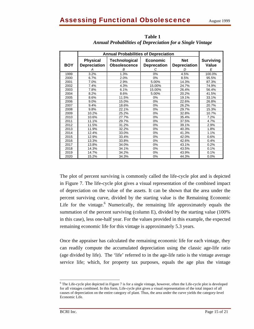
Table 1 Annual Probabilities of Depreciation for a Single Vintage
Annual Probabilities of Depreciation
BOY Physical
Depreciation Technological Obsolescence
Economic Deprecation
Net Depreciation
Surviving Value
A B C D E 1999 3.2% 1.3% 0% 4.5% 100.0% 2000 6.7% 2.0% 0% 8.5% 95.5% 2001 7.0% 2.9% 5.00% 14.3% 87.3% 2002 7.4% 4.3% 15.00% 24.7% 74.9% 2003 7.8% 6.1% 15.00% 26.4% 56.4% 2004 8.2% 8.6% 5.00% 20.2% 41.5% 2005 8.6% 11.5% 0% 19.1% 33.1% 2006 9.0% 15.0% 0% 22.6% 26.8% 2007 9.4% 18.6% 0% 26.2% 20.7% 2008 9.8% 22.1% 0% 29.7% 15.3% 2009 10.2% 25.2% 0% 32.8% 10.7% 2010 10.6% 27.7% 0% 35.4% 7.2% 2011 11.1% 29.7% 0% 37.5% 4.7% 2012 11.5% 31.2% 0% 39.1% 2.9% 2013 11.9% 32.2% 0% 40.3% 1.8% 2014 12.4% 33.0% 0% 41.3% 1.1% 2015 12.9% 33.4% 0% 42.0% 0.6% 2016 13.3% 33.8% 0% 42.6% 0.4% 2017 13.8% 34.0% 0% 43.1% 0.2% 2018 14.3% 34.1% 0% 43.5% 0.1% 2019 14.7% 34.2% 0% 43.9% 0.1% 2020 15.2% 34.3% 0% 44.3% 0.0%
The plot of percent surviving is commonly called the life-cycle plot and is depicted
in Figure 7. The life-cycle plot gives a visual representation of the combined impact
of depreciation on the value of the assets. It can be shown that the area under the
percent surviving curve, divided by the starting value is the Remaining Economic
Life for the vintage.6 Numerically, the remaining life approximately equals the
summation of the percent surviving (column E), divided by the starting value (100%
in this case), less one-half year. For the values provided in this example, the expected
remaining economic life for this vintage is approximately 5.3 years.
Once the appraiser has calculated the remaining economic life for each vintage, they
can readily compute the accumulated depreciation using the classic age-life ratio
(age divided by life). The ‘life’ referred to in the age-life ratio is the vintage average
service life; which, for property tax purposes, equals the age plus the vintage
6 The Life-cycle plot depicted in Figure 7 is for a single vintage, however, often the Life-cycle plot is developed for all vintages combined. In this form, Life-cycle plot gives a visual representation of the total impact of all causes of depreciation on the entire category of plant. Thus, the area under the curve yields the category-level Economic Life.

Assessing Functional Obsolescence August 1999
BCRI Inc. Page 16 of 21
remaining life.7 The vintage age-life ratio gives the net accumulated depreciation
resulting from all causes of depreciation considered by the appraiser.
Figure 7 Forecasted Surviving Value
(for a single vintage)
0%
10%
20%
30%
40%
50%
60%
70%
80%
90%
100%
1999 2001 2003 2005 2007 2009 2011 2013 2015
Perc
ent o
f C
urre
nt V
alue
Economic Lives Generally, it is desirable, but not necessary, to identify the corresponding economic
lives. The appraiser should be aware that the term Economic Life is used (misused) to
denote different types of lives in different disciplines, and especially aware that each
discipline is adamant that their use of the term is the correct one. Some of the more
typical life parameters are described below.
Vintage Average Service Life (VASL) – represents the average economic life of
each vintage. Due primarily to obsolescence, the VASLs are different for each
vintage. The VASL equals the realized life plus the remaining life. In depreciation
circles, the realized life is the average life realized by all equipment placed in the
vintage; including equipment that has been taken out of service and disposed of. For
appraisal purposes, only surviving equipment is considered, so the realized life is
equal to the age of the vintage.
7 Note: in depreciation circles, often the vintage average life is taken to mean the average life of all equipment
placed in that vintage – including equipment that has already been taken out of service and disposed of. For
property tax purposes, the appraiser is only interested in assessing the value of those assets existing as of the
assessment date.

Assessing Functional Obsolescence August 1999
BCRI Inc. Page 17 of 21
Economic Life (most typical context) – More often than not, the term economic life
is the expected life expectancy of newly placed equipment. It is equal to the VASL
of the newest vintage.
Projection Life – By definition, the projection life is the same as the economic life,
but in practice the term Projection Life is often more closely related to the
investment-weighted average of the VASLs.
Average Remaining Life (ARL) or Remaining Economic Life (REL) – Generally
these terms refer to the average remaining life for the entire class of property (i.e., all
vintages). The term ARL is common in depreciation circles and the term REL is
common in property tax circles. Both represent different names for the same life.
The easiest way to determine the ARL is to compute the investment weighted
average of the individual vintage remaining economic lives. Alternately, a composite
life-cycle plot may be produced and the ARL determined from the plot in the same
manor used for each vintage. This is the most common and preferred approach. It not
only provides the appraiser with a visual representation of the ongoing decline in
value of the entire class of equipment; but also provides a means to easily compute
the composite remaining life for subsequent years. The investment weighted annual
probabilities of depreciation are used to produce the composite life-cycle plot.
Final Depreciation Table For property tax purposes, accumulated depreciation is typically reflected in a
Percent Good Table (sometimes called the Depreciation Table). The Percent Good
table is a table of vintage factors that when multiplied by the original cost (or
replacement cost) for each vintage yields the remaining value. The Percent Good
factor equals one less the accumulated depreciation factor (i.e., the age-life ratio).
Alternately, the remaining value factor is computed directly from the age and life
using the following formula:
LifeRemaining_Age
LifeRemaining_ValueRemaining_
+=

Assessing Functional Obsolescence August 1999
BCRI Inc. Page 18 of 21
Most equipment has a residual value – that is, regardless of the condition of the
equipment, it has some value to the owner, if only for its junk metal content. The
Percent Good factors should not be allowed to fall below this residual value.
Residual Value Generally, all equipment has some salvage value. Discarded and defective copper
cable has some value to a copper junk dealer, for example. Likewise, discarded
circuit packs may be refurbished and resold, and when they cannot be resold, they
contain precious metals such as gold and silver that has value to the owner.
The minimum value of equipment is its Net Salvage (NS) value. NS is defined as the
Gross Salvage (GS) less the Cost of Removal. GS is the amount received from the
sale of discarded equipment; and the COR is the summation of all cost to the owner
of disposing of the equipment. The salvage factors are typically depicted as a
percentage of the original cost.
Because salvage is realized at the end of the Physical Life of the equipment, that is
when the equipment is taken out of service and discarded, the appraiser needs to
estimate the Future Net Salvage (FNS). If the remaining life is well into the future,
the FNS may be significantly different from past and current salvage values.
Generally, however, salvage trends are simple trends and do not present a problem to
the appraiser.
Once the FNS is established, the accumulated depreciation factors should not be
allowed to exceed 100 percent less the FNS percent. In terms of the Percent Good
table, the remaining value of the equipment should not be allowed to fall below the
FNS percentage. Thus, the FNS is the appraiser’s assessment of the residual value of
the equipment.
How Accurate is This Approach To Value
The author has successfully used the approach presented in this paper extensively
over the last nine years in various business applications. Some of the applications
included, property valuations (including an assessment of the entire Public

Assessing Functional Obsolescence August 1999
BCRI Inc. Page 19 of 21
Telecommunication Network in the U.S.)8, asset impairment assessments9,
depreciation assessments, economic life studies, asset management, network
planning, and long-range strategic planning.
For property valuations, ideally, the accuracy of the assessment is how close the
assessed value is to the actual value. Since there is no exact gauge for the actual
value, a surrogate is needed. The remaining economic life provides a reasonable
criterion one can use in lieu of the actual value.
The assessed value is a direct result of the projected remaining economic life. As
noted above, the percent of value remaining (Percent Good) is computed using the
age-life ratio; and equals the REL divided by the Age plus the REL. The only
estimated value in this formula is the Remaining Economic Life. Generally, the
valuation is conducted at the vintage level. The average or category-level Remaining
Economic Life is simply the investment weighted average of the vintage lives. The
category-level Economic Life provides a single measure against which one can
evaluate the accuracy of this approach to value.
The author has documented and published four case studies that compare the
estimated REL resulting from this approach to the REL actually realized. Three of
the case studies used actual mortality experience from several companies spanning
over 74 state jurisdictions and involving hundreds of thousands of units of
property.10 The fourth case study was specific to one company and one state
jurisdiction.11 The results of these case studies are summarized in Table 2.
Each case study used an effective date for the economic life near the start of
measurable Functional Obsolescence. From this date forward, the observed
Economic Life was determined from observed data collected from the FCC and from
the participating companies. The estimated Economic Life was derived using
observed data that predated the effective date of the life. In all cases, the estimated
Economic Lives were within one half year of the subsequently realized Economic
Lives.
8 S. L. Barreca, Telecommunications Infrastructure Valuation Study, 1998, Technology Futures, Inc. 9 For example, BellSouth’s multi-billion dollar asset write-down in the mid-1990s was based, in large part, on an
asset impairment study using the methodologies presented in this paper. 10 S. L. Barreca, Comparison of Economic Life Techniques, 1999, Technology Futures, Inc. 11 S. L. Barreca, Technological Obsolescence – Assessing the Loss in Value on Utility Property, 1998, Journal of the Society of Depreciation Professionals.

Assessing Functional Obsolescence August 1999
BCRI Inc. Page 20 of 21
In addition to these results, Table 2 also gives the estimated Projection Life. Here,
the term Projection Life represents the Economic Life estimate using the prevailing
life estimating techniques prescribed by the FCC and most state PSCs at that time. It
is determined by taking a recent snapshot of observed mortality characteristics.
Proponents of this approach argue that recent mortality history reflects all forms of
depreciation, including Functional Obsolescence. These results are provided to point
out the fact that while recent mortality history does, to some extent, reflect past
influences of Functional Obsolescence, it does not provide indication of future
Functional Obsolescence.
Table 2 A Case Study On The Accuracy of This Approach to Value
Case Study
Effective Date of
Life
Observed Economic
Life
Estimated Economic
Life
Estimated Projection
Life Electromechanical Switching 1980 5.1 5.6 15.7
Interoffice Underground Metallic Cable 1987 4.2 4.2 23.6
Analog Switching 1990 4.4 3.9 10.1 LEC-A, Underground Metallic Cable 1986 6.5 6.8 NA

Assessing Functional Obsolescence August 1999
BCRI Inc. Page 21 of 21
Conclusion
Functional Obsolescence is often the result of many factors, each of which
contributes to the ongoing decline in value of personal property. The net impact of
all causes of Functional Obsolescence is reflected in the reduction of the relative
usage of the property. History has shown that reductions in relative usage follow
predictable patterns; and as such, provide a means to collectively quantify the impact
of all causes of Functional Obsolescence. This paper outlines an effective Cost-based
approach to value that utilizes a combination of actuarial theory and proven
technology substitution techniques to effectively measure the collective impact of
Functional Obsolescence.
Additionally, the Cost-based approach to value presented in this paper provides a
generic approach to valuation that facilitates separately quantifying any number of
drivers of value and statistically combining them to yield the net remaining value.
Stephen L. Barreca, PE, CDP Steve has over 20 years experience in the telecommunications industry. He is a registered Professional Engineer, a Certified Depreciation Professional, and has 17 years experience assessing technological change, economic lives and property valuation. Steve has negotiated for adequate economic lives with federal and state regulators on behalf of his clients, and has testified as an expert witness in numerous valuation and rate cases in the areas of economic lives, technological change, depreciation methodology, and telecommunications network technology, methods and procedures. Steve is the Founder and President of BCRI Inc. and can be contacted at (205) 943-6710 or [email protected].
Copyright© BCRI Inc. 1999-2000, All rights reserved.