HAL Id: hal-02084842https://hal.archives-ouvertes.fr/hal-02084842

Submitted on 29 Mar 2019

HAL is a multi-disciplinary open accessarchive for the deposit and dissemination of sci-entific research documents, whether they are pub-lished or not. The documents may come fromteaching and research institutions in France orabroad, or from public or private research centers.

L’archive ouverte pluridisciplinaire HAL, estdestinée au dépôt et à la diffusion de documentsscientifiques de niveau recherche, publiés ou non,émanant des établissements d’enseignement et derecherche français ou étrangers, des laboratoirespublics ou privés.

Copyright

Asymptotic behaviour of the one-dimensional“rock-paper-scissors” cyclic cellular automaton

Benjamin Hellouin de Menibus, Yvan Le Borgne

To cite this version:Benjamin Hellouin de Menibus, Yvan Le Borgne. Asymptotic behaviour of the one-dimensional “rock-paper-scissors” cyclic cellular automaton. Annals of Applied Probability, Institute of MathematicalStatistics (IMS), In press. �hal-02084842�

Asymptotic behaviour of the one-dimensional“rock-paper-scissors” cyclic cellular automaton

Benjamin Hellouin de Menibus1 and Yvan Le Borgne2

1 Laboratoire de Recherche en Informatique,Université Paris-Sud - CNRS - CentraleSupélec, Université Paris-Saclay, France

https://orcid.org/0000-0001-5194-929X2 Univ. Bordeaux, Bordeaux INP, CNRS, LaBRI, UMR5800, F-33400 Talence, France

Abstract

The one-dimensional three-state cyclic cellular automaton is a simple spatial model with three statesin a cyclic “rock-paper-scissors” prey-predator relationship. Starting from a random configuration, similarstates gather in increasingly large clusters; asymptotically, any finite region is filled with a uniform statethat is, after some time, driven out by its predator, each state taking its turn in dominating the region(heteroclinic cycles).

We consider the situation where each site in the initial configuration is chosen independently atrandom with a different probability for each state. We prove that the asymptotic probability that a statedominates a finite region corresponds to the initial probability of its prey. The proof methods are basedon discrete probability tools, mainly particle systems and random walks.

Keywords: cyclic dominance, heteroclinic cycles, cellular automata, self-organisation, random walk

Cyclic dominance is a general term for phenomena where different states (species, strategies, etc.) are inprey-predator relationships that form a cycle: A preys on B preys on C. . . preys on A. This phenomenonoccurs in many natural or theoretical systems, among which a few examples are:

Population ecology male mating strategies in side-blotched lizard [27], antibiotic production and resis-tance in E.Coli [18], parasite-grass-forb interactions [5], oscillations in the population size of pacificsalmon [12], etc.

Game theory pure or stochastic strategies in rock-paper-scissors type games, iterated prisoner’s dilemma[26, 15], public goods games [13, 24], etc.

Infection models The SIRS compartmental model [1] (susceptible / infectious / recovered, when a recov-ered agent may become susceptible again), forest fire models [2], etc.

Many additional examples can be found in [29] (section 7) and [30].May and Leonard’s [21] is the first effort to model the evolution of three species with cyclic dominance,

using the standard Lotka-Volterra equations; it is a mean-field approximation, that is, it assumes the popu-lation is well-mixed. The system exhibits so-called heteroclinic cycles where each species in turn dominatesalmost the whole space before being replaced by its predator. Consequently, cyclic dominance has beenproposed as a mechanism to explain the coexistence of various strategies or species [17] (biodiversity), theregular oscillations in population sizes of different species [12], and some counter-intuitive phenomena suchas the “survival of the weakest” [11]. In other contexts, heteroclinic cycles appear to coincide with importantconcepts: for example, social choice among three cyclically dominant choices can lead to an heteroclinic cyclealong the so-called bipartisan set [19].

1

Mean-field models do not take into account spatial aspects of the evolution of populations, such as theeffect of population structure, mobility, dispersal, local survival, etc. This is why spatial models have beenintroduced both in ecology [6, 31] and in so-called evolutionary game theory [29]. In both cases agents havea spatial location and can only interact with their neighbours at short range. There is some variety in spatialmodels:

Space a lattice in one, two or more dimensions, or a graph with more structure;

Updates discrete or continuous time, synchronous or asynchronous updates;

Dynamics usually a predator replaces a prey by a copy of itself (replicator dynamics). The model caninclude empty space, different ranges, threshold effects, invasion probabilities, etc.;

Boundaries infinite, periodic or fixed boundary conditions, choice of the initial configuration.

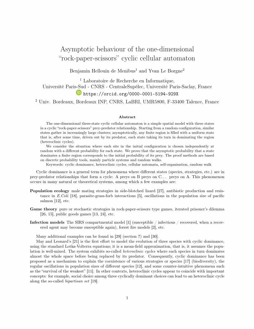
In this article, we consider arguably the simplest spatial model for cyclic dominance: the one-dimensional,3-state cyclic cellular automaton. Each site on the lattice Z is initially associated a state in Z/3Z. At each(discrete) time step, every site is updated synchronously: if any of the two neighbouring sites contains apredator, it becomes the new state for this site. While the restriction to one dimension may not be ecologicallyrealistic (two-dimensional models being the object of more interest [31]), it has two benefits. First, its simplespatial structure makes many questions mathematically tractable, while the two-dimensional models havemuch more complex dynamics with structured interfaces between regions [7]. Second, its dynamics is similarto a interacting particle system with borders progressing at constant speed and annihilating on contact(ballistic annihilation - see Figure 1); this is a subject of independent interest [4] and many tools have beendeveloped for it [3].

Figure 1: (Left) The 3-state cyclic cellular automaton; (Right) The dynamics of its particles.

Note In all space-time diagrams of this article, the initial configuration is drawn horizontally at the bottomand time goes from bottom to top. States are represented by colours following the convention 0 7→ �, 1 7→�, 2 7→ �, 3 7→ �, 4 7→ �.

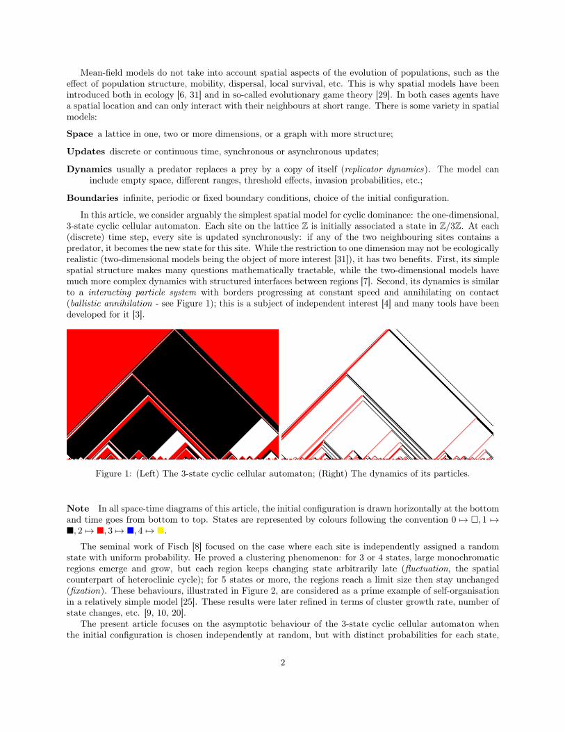
The seminal work of Fisch [8] focused on the case where each site is independently assigned a randomstate with uniform probability. He proved a clustering phenomenon: for 3 or 4 states, large monochromaticregions emerge and grow, but each region keeps changing state arbitrarily late (fluctuation, the spatialcounterpart of heteroclinic cycle); for 5 states or more, the regions reach a limit size then stay unchanged(fixation). These behaviours, illustrated in Figure 2, are considered as a prime example of self-organisationin a relatively simple model [25]. These results were later refined in terms of cluster growth rate, number ofstate changes, etc. [9, 10, 20].

The present article focuses on the asymptotic behaviour of the 3-state cyclic cellular automaton whenthe initial configuration is chosen independently at random, but with distinct probabilities for each state,

2

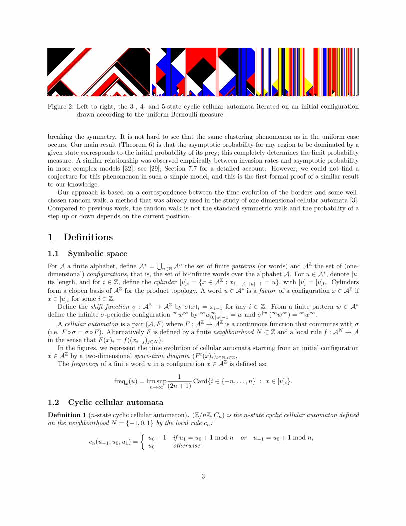
Figure 2: Left to right, the 3-, 4- and 5-state cyclic cellular automata iterated on an initial configurationdrawn according to the uniform Bernoulli measure.

breaking the symmetry. It is not hard to see that the same clustering phenomenon as in the uniform caseoccurs. Our main result (Theorem 6) is that the asymptotic probability for any region to be dominated by agiven state corresponds to the initial probability of its prey; this completely determines the limit probabilitymeasure. A similar relationship was observed empirically between invasion rates and asymptotic probabilityin more complex models [32]; see [29], Section 7.7 for a detailed account. However, we could not find aconjecture for this phenomenon in such a simple model, and this is the first formal proof of a similar resultto our knowledge.

Our approach is based on a correspondence between the time evolution of the borders and some well-chosen random walk, a method that was already used in the study of one-dimensional cellular automata [3].Compared to previous work, the random walk is not the standard symmetric walk and the probability of astep up or down depends on the current position.

1 Definitions

1.1 Symbolic spaceFor A a finite alphabet, define A∗ =

⋃n∈NAn the set of finite patterns (or words) and AZ the set of (one-

dimensional) configurations, that is, the set of bi-infinite words over the alphabet A. For u ∈ A∗, denote |u|its length, and for i ∈ Z, define the cylinder [u]i = {x ∈ AZ : xi,...,i+|u|−1 = u}, with [u] = [u]0. Cylindersform a clopen basis of AZ for the product topology. A word u ∈ A∗ is a factor of a configuration x ∈ AZ ifx ∈ [u]i for some i ∈ Z.

Define the shift function σ : AZ → AZ by σ(x)i = xi−1 for any i ∈ Z. From a finite pattern w ∈ A∗define the infinite σ-periodic configuration ∞w∞ by ∞w∞0,|w|−1 = w and σ|w|(∞w∞) = ∞w∞.

A cellular automaton is a pair (A, F ) where F : AZ → AZ is a continuous function that commutes with σ(i.e. F ◦σ = σ ◦F ). Alternatively F is defined by a finite neighbourhood N ⊂ Z and a local rule f : AN → Ain the sense that F (x)i = f((xi+j)j∈N ).

In the figures, we represent the time evolution of cellular automata starting from an initial configurationx ∈ AZ by a two-dimensional space-time diagram (F t(x)i)t∈N,i∈Z.

The frequency of a finite word u in a configuration x ∈ AZ is defined as:

freqx(u) = lim supn→∞

1

(2n+ 1)Card{i ∈ {−n, . . . , n} : x ∈ [u]i}.

1.2 Cyclic cellular automataDefinition 1 (n-state cyclic cellular automaton). (Z/nZ, Cn) is the n-state cyclic cellular automaton definedon the neighbourhood N = {−1, 0, 1} by the local rule cn:

cn(u−1, u0, u1) =

{u0 + 1 if u1 = u0 + 1 mod n or u−1 = u0 + 1 mod n,u0 otherwise.

3

All operations concerning n-state cyclic automata are assumed to be modulo n.

As should be clear from Figure 2, the self-organisation is driven by borders between monochromaticregions behaving as particles. We call particles the factors ab of length 2 (with a 6= b) in a configuration.Each particle moves “from predator to prey”, that is, left if a = b + 1, right if b = a + 1, and stays putotherwise. This motivates the following definitions:

Positive particles p+ = {ab : b = a+ 1};

Negative particles p− = {ab : b = a− 1};

Neutral particles p= = {ab : b /∈ {a− 1, a, a+ 1}}.

and we write [p+]i as a shorthand for⋃ab∈p+ [ab]i: it means that a positive particle occurs at position i.

Notice that p= = ∅ for n = 3. Figure 1 illustrate the particle dynamics for n = 3.

1.3 Probability measures on AZ

Let B be the Borel sigma-algebra of AZ. Denote byM(AZ) the set of probability measures on AZ definedon the sigma-algebra B. Since the cylinders {[u]n : u ∈ A∗, n ∈ Z} form a basis of the product topologyon AZ, a measure µ ∈M(AZ) is entirely characterised by the values µ([u]n).

In this paper, we only consider σ-invariant probability measures, and therefore write µ([u]) instead ofµ([u]n).

Examples.

Measures supported by a periodic orbit For a word w ∈ A∗, we define the σ-invariant measure sup-ported by ∞w∞ by taking the mean of the Dirac measures δ∞w∞ along its σ-orbit:

δ∞w∞ =1

|w|∑

i∈[0,|w|−1]

σi(δ∞w∞).

When w is a single letter a, we obtain the measure supported on the single monochromatic configuration∞a∞.

Bernoulli measure Let v = (va)a∈A be a vector of real numbers such that 0 ≤ va ≤ 1 for all a ∈ A and∑a∈A va = 1. Let βv be the discrete probability distribution on A such that βv(a) = va for all a ∈ A

(a generalisation of the standard Bernoulli law with n outcomes).The associated Bernoulli measure Berv on AZ is the product measure

∏i∈Z βv, that is,

Berv([u0 . . . un]) = vu0· · · vun

for all u0 . . . un ∈ A∗.

In other words, each cell is drawn in an i.i.d. manner according to βv. We denote Ber(AZ) the set ofBernoulli measures on AZ with nonzero parameters (va)a∈A.

Uniform measure In particular, if we take va = 1|A| for all a ∈ A in the previous definition, we obtain the

uniform (Bernoulli) measure λ.

The image measure of µ ∈ Mσ(AZ) by a cellular automaton (AZ, F ) is defined as Fµ(B) = µ(F−1(B))for all B ∈ B. This defines an action F :Mσ(AZ)→Mσ(AZ).

We endow Mσ(AZ) with the weak∗ topology : for a sequence (µn)n∈N ∈ Mσ(AZ)N and a measure µ ∈Mσ(AZ), we have µn −→

n→∞µ if, and only if:

∀u ∈ A∗, µn([u]) −→n→∞

µ([u]).

4

This topology makes F continuous andMσ(AZ) is compact.A measure µ ∈Mσ(AZ) is σ-ergodic if, for every subset S ⊂ AZ such that σ(S) = S µ-almost everywhere,

we have µ(S) = 0 or 1. The set of σ-ergodic measures is denotedMergσ (AZ). In particular, all examples above

are σ-ergodic and the image of a σ-ergodic measure under the action of a cellular automaton is σ-ergodic.As an example of a non-σ-ergodic measure, consider the average of two Dirac measures 1

2 (δ∞0∞ + δ∞1∞)

(the set {∞0∞} is σ-invariant and has measure 12 ).

We make use of the following corollary to Birkhoff’s theorem:

Corollary 2. Let µ ∈Mergσ (AZ) and u ∈ A∗. Then:

∀µx ∈ AZ, freq(u, x) = µ([u])

where ∀µx means for µ-almost all x (that is, for all x in some set of measure 1).

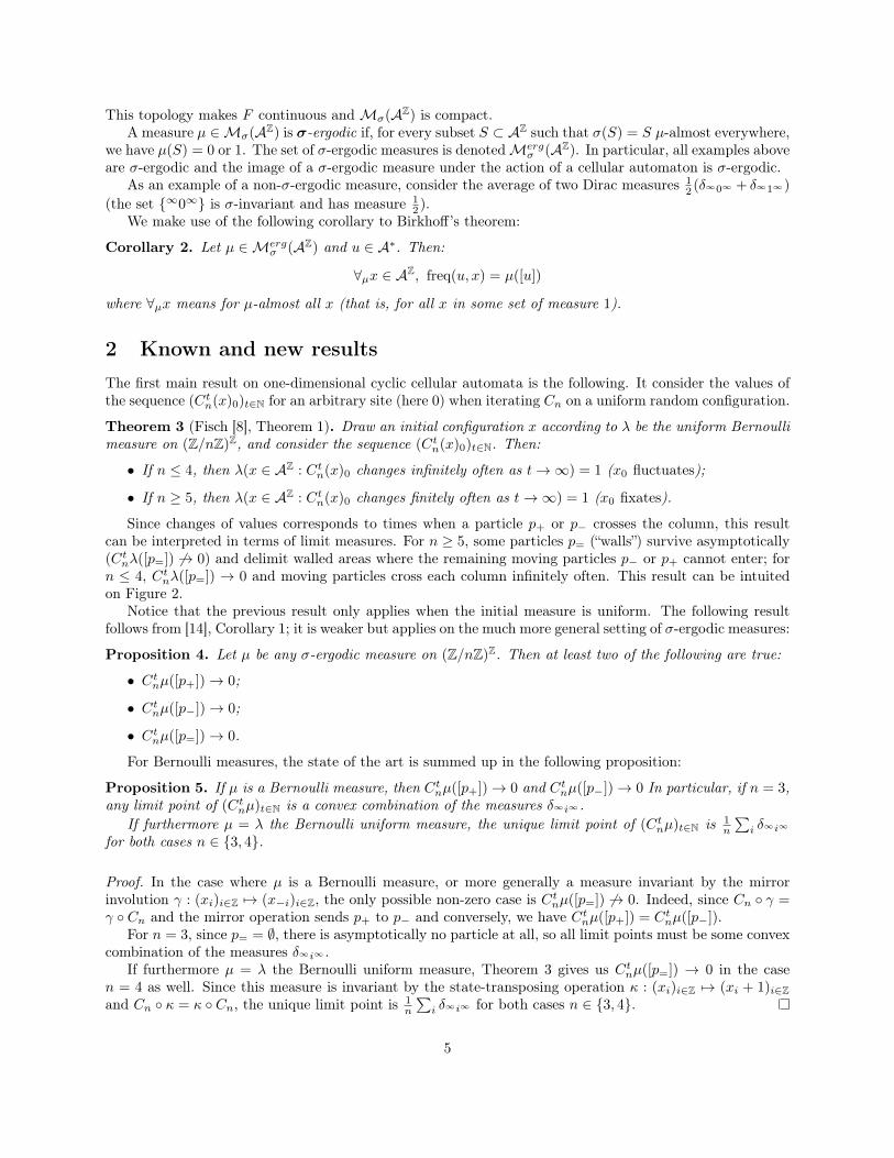
2 Known and new resultsThe first main result on one-dimensional cyclic cellular automata is the following. It consider the values ofthe sequence (Ctn(x)0)t∈N for an arbitrary site (here 0) when iterating Cn on a uniform random configuration.

Theorem 3 (Fisch [8], Theorem 1). Draw an initial configuration x according to λ be the uniform Bernoullimeasure on (Z/nZ)Z, and consider the sequence (Ctn(x)0)t∈N. Then:

• If n ≤ 4, then λ(x ∈ AZ : Ctn(x)0 changes infinitely often as t→∞) = 1 (x0 fluctuates);

• If n ≥ 5, then λ(x ∈ AZ : Ctn(x)0 changes finitely often as t→∞) = 1 (x0 fixates).

Since changes of values corresponds to times when a particle p+ or p− crosses the column, this resultcan be interpreted in terms of limit measures. For n ≥ 5, some particles p= (“walls”) survive asymptotically(Ctnλ([p=]) 6→ 0) and delimit walled areas where the remaining moving particles p− or p+ cannot enter; forn ≤ 4, Ctnλ([p=]) → 0 and moving particles cross each column infinitely often. This result can be intuitedon Figure 2.

Notice that the previous result only applies when the initial measure is uniform. The following resultfollows from [14], Corollary 1; it is weaker but applies on the much more general setting of σ-ergodic measures:

Proposition 4. Let µ be any σ-ergodic measure on (Z/nZ)Z. Then at least two of the following are true:

• Ctnµ([p+])→ 0;

• Ctnµ([p−])→ 0;

• Ctnµ([p=])→ 0.

For Bernoulli measures, the state of the art is summed up in the following proposition:

Proposition 5. If µ is a Bernoulli measure, then Ctnµ([p+])→ 0 and Ctnµ([p−])→ 0 In particular, if n = 3,any limit point of (Ctnµ)t∈N is a convex combination of the measures δ∞i∞ .

If furthermore µ = λ the Bernoulli uniform measure, the unique limit point of (Ctnµ)t∈N is 1n

∑i δ∞i∞

for both cases n ∈ {3, 4}.

Proof. In the case where µ is a Bernoulli measure, or more generally a measure invariant by the mirrorinvolution γ : (xi)i∈Z 7→ (x−i)i∈Z, the only possible non-zero case is Ctnµ([p=]) 6→ 0. Indeed, since Cn ◦ γ =γ ◦ Cn and the mirror operation sends p+ to p− and conversely, we have Ctnµ([p+]) = Ctnµ([p−]).

For n = 3, since p= = ∅, there is asymptotically no particle at all, so all limit points must be some convexcombination of the measures δ∞i∞ .

If furthermore µ = λ the Bernoulli uniform measure, Theorem 3 gives us Ctnµ([p=]) → 0 in the casen = 4 as well. Since this measure is invariant by the state-transposing operation κ : (xi)i∈Z 7→ (xi + 1)i∈Zand Cn ◦ κ = κ ◦ Cn, the unique limit point is 1

n

∑i δ∞i∞ for both cases n ∈ {3, 4}.

5

The previous results, fluctuation in particular, can be interpreted in terms of heteroclinic cycles. Forλ-almost every configuration x, no state ever dominates the whole space in the sense that (by Corollary 1)freq(i, Ct3(x)) = Ct3λ[i]→ 1

3 for every state i ∈ Z/3Z (we use the fact that the image under C3 of a σ-ergodicmeasure is σ-ergodic).

However, Proposition 5 implies that, for any fixed window [−N,N ] and λ-almost every x, Ct3(x)[−N,N ] ismonochromatic (in topological terms, it is close to one of the ∞i∞, i ∈ Z/3Z) except for some sequence oftimes of zero density. Theorem 3 further shows that Ct3(x) does not converge to one of the ∞i∞ as t→∞,but that the window keeps changing state (as a particle crosses the central column), less and less often,letting each state dominate the central window in turn. In this sense, the 3-state cyclic cellular automatonexhibits heteroclinic cycles in local regions.

Our main new result determines the unique limit point for non-uniform Bernoulli measures:

Theorem 6 (Main result).Let µ be a Bernoulli measure on (Z/3Z)Z with nonzero parameters (p0, p1, p2). Then:

Ct3µ −→t→∞

p2δ∞0∞ + p0δ∞1∞ + p1δ∞2∞ .

Theorem 6 can be interpreted as follows. Draw an initial configuration according to a Bernoulli measurewith nonzero parameters (p0, p1, p2), and consider a fixed arbitrary window [−N,N ]. By Proposition 5, theprobability that Ct3(x)[−N,N ] contains at least two different states (i.e. a particle) tends to 0. Theorem 6further shows that the probability that Ct3(x)[−N,N ] = i2N+1 for i ∈ Z/3Z tends to pi−1 as t tends to infinity.

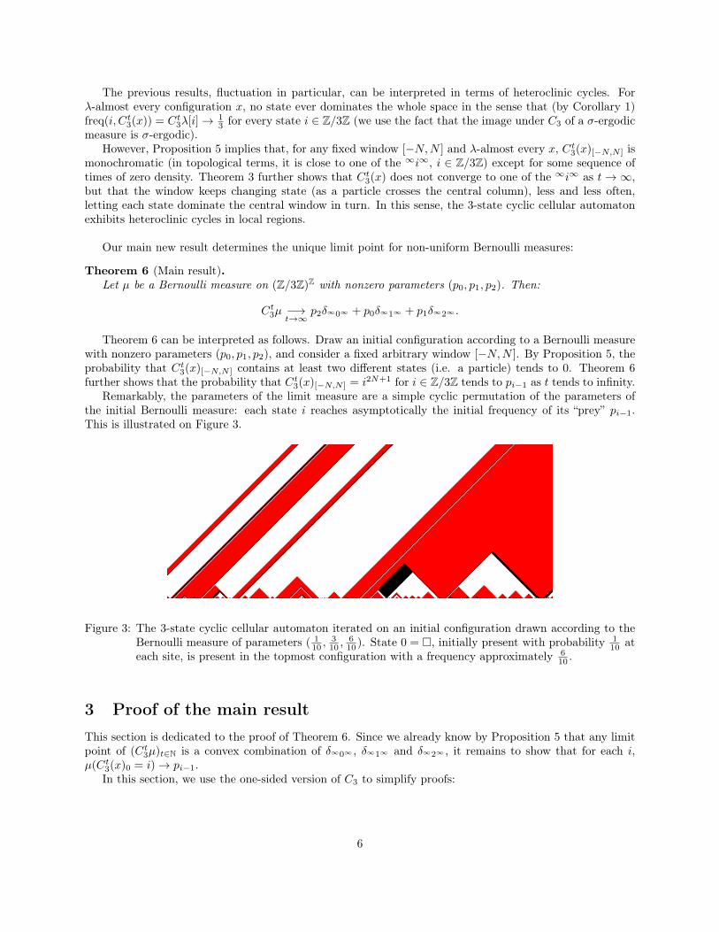
Remarkably, the parameters of the limit measure are a simple cyclic permutation of the parameters ofthe initial Bernoulli measure: each state i reaches asymptotically the initial frequency of its “prey” pi−1.This is illustrated on Figure 3.

Figure 3: The 3-state cyclic cellular automaton iterated on an initial configuration drawn according to theBernoulli measure of parameters ( 1

10 ,310 ,

610 ). State 0 = �, initially present with probability 1

10 ateach site, is present in the topmost configuration with a frequency approximately 6

10 .

3 Proof of the main resultThis section is dedicated to the proof of Theorem 6. Since we already know by Proposition 5 that any limitpoint of (Ct3µ)t∈N is a convex combination of δ∞0∞ , δ∞1∞ and δ∞2∞ , it remains to show that for each i,µ(Ct3(x)0 = i)→ pi−1.

In this section, we use the one-sided version of C3 to simplify proofs:

6

Definition 7 (One-sided cyclic CA). (Z/3Z, C3+) is the one-sided 3-state cyclic cellular automaton definedon the neighbourhood N = {0, 1} by the local rule:

c3+(u0, u1) =

{u0 + 1 if u1 = u0 + 1 mod n,u0 otherwise.

A (computer assisted) proof by enumeration of all 33 = 27 factors of length 3, shows that

C3 = C23+ ◦ σ.

Hence proving Theorem 6 on C3+ implies a similar result on C3.The proof proceeds in 4 steps:

Section 3.1 where we associate a random walk to each configuration and relate the properties of thisrandom walk to the orbit of the configuration under C3+;

Section 3.2 where we translate Theorem 6 on the random walk and establish the objects that will berelevant to the proof.

Section 3.3 where we introduce a second random walk “embedded” in the previous one, which is symmetric(hence easier to analyse) and captures its large-scale behaviour.

Section 3.4 where we bring back the results from the embedded walk to the initial walk and bring all toolstogether to conclude the proof.

3.1 Random walk associated with a configurationIn this section, we introduce tools to turn the study of the dynamics of the 3-state cyclic automaton, inparticular of Ct3+(x)0 (defined above), into the study of some random walk built from the initial configurationx.

Definition 8. To a configuration x ∈ {0, 1, 2}Z we associate a random walk W [x] := (wi)i∈Z on Z such thatw0 ∈ {0, 1, 2} and made up of steps in {−1, 0, 1} as follows:

• w0 = x0,

• for all i ≥ 0, wi+1 is the value in {wi − 1, wi, wi + 1} such that wi+1 ≡ xi+1 mod 3,

• and for i ≤ 0, wi−1 is the value in {wi − 1, wi, wi + 1} such that wi−1 ≡ xi−1 mod 3.

and this encoding is an injection.

Figure 4 provides an example of this encoding (black configuration to black walk).We denote byW[a,b][x] := (wa, wa+1, . . . , wb) the positions of the walk on Z from time a to time b. Notice

that we call time in the context of the random walk what corresponds to space in the configuration x, whichis different from the time corresponding to the iteration of cellular automaton. Context should make clearwhich notion of time we refer to.

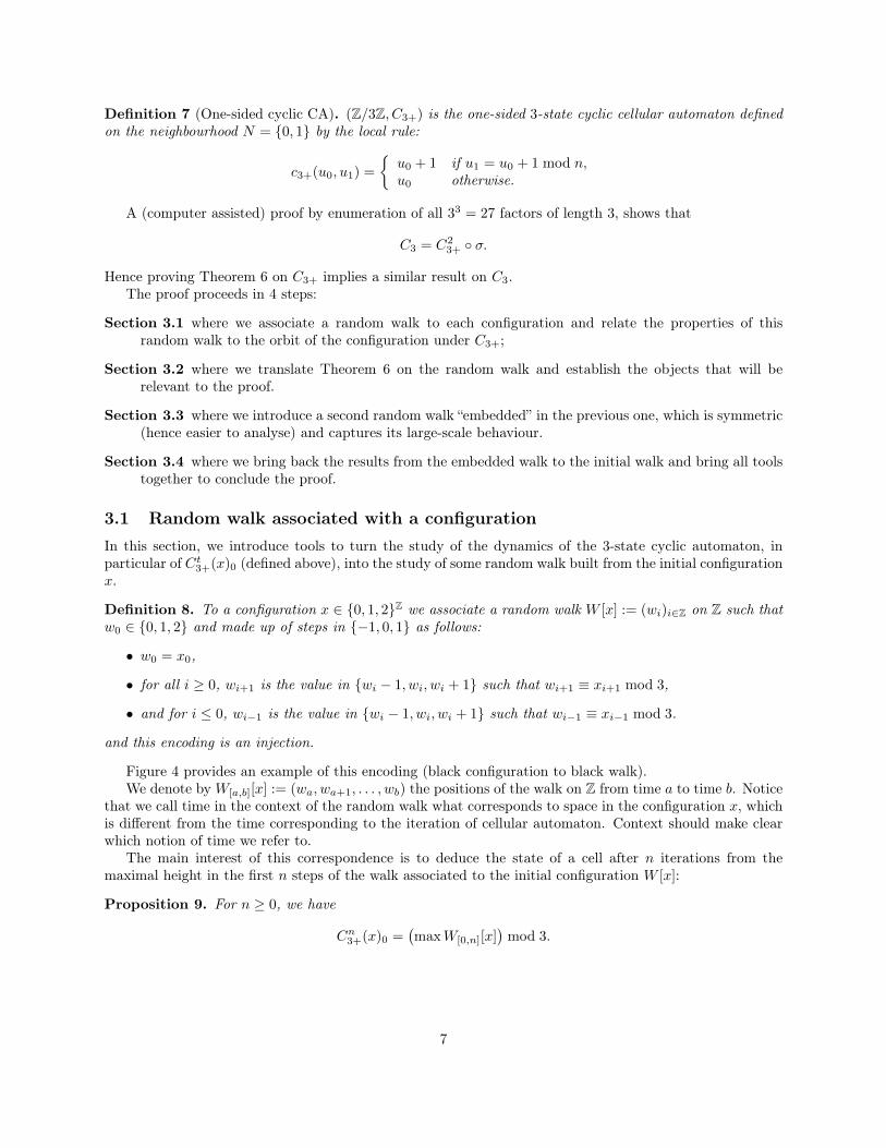
The main interest of this correspondence is to deduce the state of a cell after n iterations from themaximal height in the first n steps of the walk associated to the initial configuration W [x]:

Proposition 9. For n ≥ 0, we have

Cn3+(x)0 =(maxW[0,n][x]

)mod 3.

7

Proof. We will prove that the iterations of C3+ keep for t = 0, . . . n− 1 the following invariant:(maxW[0,n−t][C

t3+(x)]

)mod 3 =

(maxW[0,n−(t+1)][C

t+13+ (x)]

)mod 3.

When this invariant is expressed for t = 0 and t = n, we deduce the expected identity:(maxW[0,n][x]

)mod 3 =

(maxW[0,0][C

n3+(x)]

)mod 3 = max{Cn3+(x)0} mod 3 = Cn3+(x)0.

We prove this invariant in the case t = 0 and any n ≥ 1. The cases t > 0 follow by replacing x := Ct3+(x)and n := n− t.

We describe how to obtain W[0,n−1][C3+(x)] = (w′i)i=0,...,n =: w′ from W[0,n][x] = (wi)i=0,...,n+1 =: wby a 3-step transformation: w 7→ w1 := (w1

i )i=0,...n+1 7→ w2 := (w2i )i=0,...n+1 7→ w′. Each of these steps,

illustrated in Figure 4, preserves the invariant.

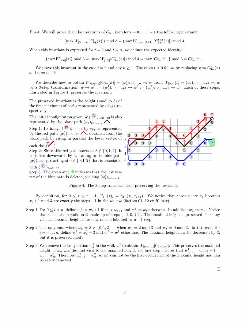
The preserved invariant is the height (modulo 3) ofthe first maximum of paths represented by , , , re-spectively.The initial configuration given by ( xi )i=0...12 is alsorepresented by the black path (wi)i=0...12 .

Step 1: Its image (yi )i=0...12 by c3+ is represented

by the red path (w1i )i=0...12 , obtained from the

black path by rising in parallel the lower vertex of

each rise ( ).Step 2: Since this red path starts at 3 /∈ {0, 1, 2}, itis shifted downwards by 3, leading to the blue path(w2

i )i=0...12 starting at 0 ∈ {0, 1, 2} that is associatedwith (

yi )i=0...12.Step 3: The green area indicates that the last ver-tex of the blue path is deleted, yielding (w′i)i=0...11.

2

0 0 0

1

2

1

0

2

0

1

2

0

0

1

2

30 0 0

1

2 2

1

0 0

1

2

0 ?

0 0 0

1

2 2

1

0 0

1

2

0 ?

Figure 4: The 3-step transformation preserving the invariant.

By definition, for 0 ≤ i ≤ n − 1, C3+(x)i = c3+(xi, xi+1). We notice that cases where xi becomesxi + 1 mod 3 are exactly the steps +1 in the walk w (factors 01, 12 or 20 in x).

Step 1 For 0 ≤ i < n, define w1i := wi + 1 if wi < wi+1 and w1

i := wi otherwise. In addition w1n := wn. Notice

that w1 is also a walk on Z made up of steps {−1, 0,+1}. The maximal height is preserved since anyvisit at maximal height in w may not be followed by a +1 step.

Step 2 The only case where w10 = 3 /∈ {0, 1, 2} is when w0 = 2 mod 3 and w1 = 0 mod 3. In this case, for

i = 0, . . . n, define w2i = w1

i − 3 and w2 = w1 otherwise. The maximal height may be decreased by 3,but it is preserved mod3.

Step 3 We remove the last position w2n in the walk w2 to obtainW[0,n−1][C3+(x)]. This preserves the maximal

height: if wn was the first visit to the maximal height, the first step ensures that w1n−1 = wn−1 + 1 =

wn = w1n. Therefore w2

n−1 = w2n, so w2

n can not be the first occurrence of the maximal height and canbe safely removed.

8

3.2 Analysing the random walkRecall that the measure on the initial configuration is the Bernoulli measure µ of parameters (p0, p1, p2).From this and the bijection with walks on Z we forget its relationship with x to study it for itself as a randomvariable, directly sampling W [x] as follows (each choice being independent):

• w0 = j with probability pj for j ∈ {0, 1, 2},

• then for all i ≥ 0, with probability pj , wi+1 is the value in {wi−1, wi, wi+1} such that wi+1 ≡ j mod 3for j ∈ {0, 1, 2},

• and for i ≤ 0, with probability pj , wi−1 is the value in {wi − 1, wi, wi + 1} such that wi−1 ≡ j mod 3for j ∈ {0, 1, 2}.

Similarly, we can sample the factor W[0,n][x] = (wi)i=0,...n by assuming by convention that w−1 = 1 toensure that w0 ∈ {0, 1, 2}. Then the only rule is wi+1 ∈ {wi − 1, wi, wi + 1} with probability pwi+1 mod 3,independently from other choices.

In the proofs, we will need such walks starting from an arbitrary k ∈ Z. Formally, define Wk,n a randomwalk on Z of length n ∈ N and starting from k ∈ Z as:

Wk,n := (Wt)t=0...n where W0 = kWt = Wt−1 − 1 + ((Zt −Wt−1 + 1) mod 3) for t = 1 . . . n,

where (Zt)t=1...n are i.i.d. random variables in Z/3Z := {0, 1, 2} for all t, and P(Zt = j) = pj for all j ∈ Z/3Z.

Theorem 10 (Main result of this section). For any i ∈ Z/3Z and any k ∈ Z,

limn→+∞

P(max(Wk,n) mod 3 = i) = p(i−1) mod 3

where max(Wk,n) := maxt=0...n

Wt.

We first consider the case i = 0 (and k = 0), i.e. limn→+∞ P(max(W0,n) mod 3 = 0) = p2; the othercases will follow.

Our proof proceeds by conditioning this event to the lengthm of the 3-tail (defined below), and describingthe probability in terms of the value of other probabilities (P<Hk,m )k,m,H (also defined below).

Definition 11 (Record, tail). A record occurs at time t′ in the random walk Wk,n if Wt′ = maxt=0...t′Wt;notice a walk can have multiple records ti sharing the same value Wti .

The h-tail of Wk,n is the suffix W[t′...n], where t′ is the last occurrence of a record Wt′ divisible by h; theh-tail for h > 1 may not exist.

We make use of the 3-tail and the 1-tail in the proof. The length of the 3-tail tail3(Wk,n) := n − t′ isusually denoted by m.

Notations:

• W<Hk,n is the set of walks on n ∈ N steps which start from k ∈ Z and remain on values strictly lower

than H ∈ Z.

• P<Hk,n is the probability that a random walk Wk,n belongs to W<Hk,n .

Proposition 12 (Description conditioned by 3-tail). For any n ∈ N and any possible 3-tail length m ≥ 1,we have:

P(max(Wk,n) mod 3 = 0 | tail3(Wk,n) = m) = p2Km

where Km :=P<0−1,m−1

P<0−1,m

.

9

Proof. By the definition of conditional probability:

P(max(Wk,n) mod 3 = 0 | tail3(Wk,n) = m) =P(tail3(Wk,n) = m and max(Wk,n) mod 3 = 0)

P(tail3(Wk,n) = m).

We now evaluate the denominator and then the numerator of the right-hand side.

Evaluation of P(tail3(Wk,n) = m):By definition tail3(Wk,n) = m > 1 implies that Wn−m = 3H is the last record divisible by 3 in Wk,n,

and that Wn−m+1 exists and is in the 3-tail. Assume therefore that Wn−m = 3H for some H. Since m ≥ 1,we may discuss the possible values of Wn−m+1 ∈ {3H − 1, 3H, 3H + 1} for any walk of Wk,n. We identifybelow which of these values are allowed.

• IfWn−m+1 = 3H (with probability p0), thenWn−m is not the last record divisible by 3, a contradiction.

• IfWn−m+1 = 3H+1 (with probability p1), future visits of height 3H will not be a new record, soWn−mis the last record divisible by 3 if and only if the walk never reaches 3H + 3 (the next record divisibleby 3). This corresponds to W[n−m+1,...n] ∈W<3H+3

3H+1,m−1 happening with probability P<3H+33H+1,m−1.

• If Wn−m+1 = 3H − 1 (with probability p2), the next visit of height 3H would be a new occurrence ofa record divisible by 3, so Wn−m is the last record divisible by 3 if and only if the walk never reachesagain 3H. This corresponds to W[n−m+1,...n] ∈W<3H

3H−1,m−1 happening with probability P<3H3H−1,m−1.

In the definition of Wk,n it appears that any realisation (Wt)t ∈ Wk,n can be translated into (Wt + 3T )t forany T ∈ Z without changing the probability of steps. This implies that for any 3T ∈ 3Z we have

∀H, k ∈ Z2,∀n ∈ N, P<Hk,n = P<H+3Tk+3T,n .

Therefore the probabilities in the previous discussion does not depend on 3H. By the law of total probability:

P(tail3(Wk,n) = m) =∑H∈Z

P(Wn−m = 3H) · P(tail3(Wk,n) = m | Wn−m = 3H)

=∑H∈Z

P(Wn−m = 3H) · (p1P<3H+33H+1,m−1 + p2P

<3H3H−1,m−1)

= P(Wn−m = 0 mod 3) · (p1P<0−2,m−1 + p2P

<0−1,m−1)

= p0 · (p1P<0−2,m−1 + p2P

<0−1,m−1)

where we use the fact that any step in the walk leads to a height divisible by 3 with probability p0, regardlessof the previous position.

The first step of a walk in W<0−1,m leads from −1 to either −1 or −2, so we get the following partition:

W<0−1,m = {−1} ×W<0

−1,m−1 ∪ {−1} ×W<0−2,m−1

In terms of probabilities this identity turns into:

P<0−1,m = p2P

<0−1,m−1 + p1P

<0−2,m−1.

Hence P(tail3(Wk,n) = m) = p0P<0−1,m.

Evaluation of P(tail3(Wk,n) = m and max(Wk,n) mod 3 = 0): We reconsider the previous discussion onWn−m+1 under the additional condition max(Wk,n) mod 3 = 0. Again assume that Wn−m = 3H

• Wm−n+1 = 3H is still impossible by definition of the 3-tail.

10

• Wm−n+1 = 3H+1 is impossible since it would imply the maximum is strictly greater that 3H. However,no new record divisible by three is now reachable by definition of 3-tail.

Hence the only possible choice for Wn−m+1 is 3H − 1, and the walk must avoid 3H from time n−m+ 1onwards: this happens with probability p2P<3H

3H−1,m−1 = p2P<0−1,m−1. Therefore the numerator of Km is

P(tail3(Wk,n) = m and max(Wk,n) mod 3 = 0) = p0p2P<0−1,m−1

Since by assumption p0 6= 0, they cancel out in the expression for Km to give the desired result.

3.3 The embedded walkThe remainder of this section proves that when n tends to infinity, the length m of the 3-tail also tends toinfinity with high probability (Lemma 17) and Km tends to 1 (Lemma 18). Proposition 12 then leads toTheorem 10 for i = 0 asymptotically.

We use a factorisation of the walk into factors forming a symmetric {+3,−3} random walk on 3Z, thatcan be scaled to be the usual symmetric {+1,−1} random walk on Z.

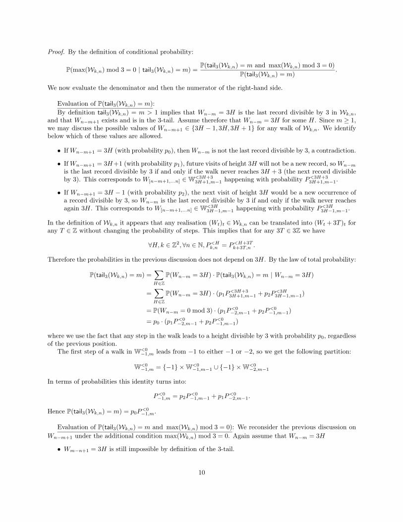
Definition 13 (Embedded walk). Define greedily and recursively a sequence of times (tj)j=0,...J−1 as follows:

• Wt0 is the first occurrence of a value divisible by 3 in Wk,n, if any.

• given (tj)j=0,...i−1, ti is the next time where Wti is divisible by 3 and distinct from Wti−1, if any such

ti ≤ n exists.

From this sequence we define the embedded random walk Wsk,n = (Wtj )j=0...J−1 whose length J , also

denoted |Wsk,n|, is random.

An example of embedded walk is given in Figure 5.

−3

−2

−1

0

1

2

3

4

5

6

0 1 2 3 4 5 6 7 8 9 10 11 12 13 14 15 16 17 18 19 20 21 22 23 24 25 26 27

t0

t1

t2

t3

t4

t5

Figure 5: A (black) walk W1,27 of length 27 and its embedded (red) walk Ws1,27 of length J = 6.

First we show that the embedded walk on 3Z is symmetric (Lemma 14), then that its length is at leastlinear in the size of the original walk with high probability (Lemma 15) and finally provide a upper boundon the probability of a small 1-tail in this symmetric {+1,−1} walk on Z (Lemma 16).

Lemma 14 (The embedded walk on 3Z is symmetric). For any value J ≥ 0 and any n ≥ 0, the walk Wsk,n

conditioned by |Wsk,n| = J is a symmetric random walk of J − 1 steps1 {−3,+3} on 3Z with independent

steps.1By convention, 0 steps means one vertex, −1 steps means no vertex at all.

11

Proof. The vertex Wt0 exists since the length of the embedded walk is conditioned to be J ≥ 0. We provethat Ws

k,n is symmetric, that is, for any i such that 1 ≤ i ≤ J − 1:

P(Wti = Wti−1+ 3) = P(Wti = Wti−1

− 3)

The proof of this equality relies on an involution on the atomic events (Zk)k=ti−1+1,...,ti =: Z]ti−1,ti] describingthe two probabilities. We illustrate this involution on Figure 6.

First denote, for any a < b, Z ]a,b] = (Za+b+1−k)k=a+1,...b the mirror image of the sequence Z]a,b]. Second,for any sequence Z]ti−1,ti] defining an event where Wti = Wti−1

+ 3, define si as the index of the lastoccurrence of the event Zt = 0 (that is, Wt = 0 mod 3) before ti; notice si ≥ ti−1 since Zti−1

= 0. It appearsthat the map

τ : Z]ti−1,ti] = Z]ti−1,si]Z]si,ti−1]Zti −→ Z]ti−1,si]Z ]si,ti−1]Zti

is an involution from the events where Wti = Wti−1 + 3 to the events where Wti = Wti−1 − 3 (see moredetails in Figure 6). Furthermore, since Z]a,b] and Z ]a,b] have the same probability, τ preserves probabilities.

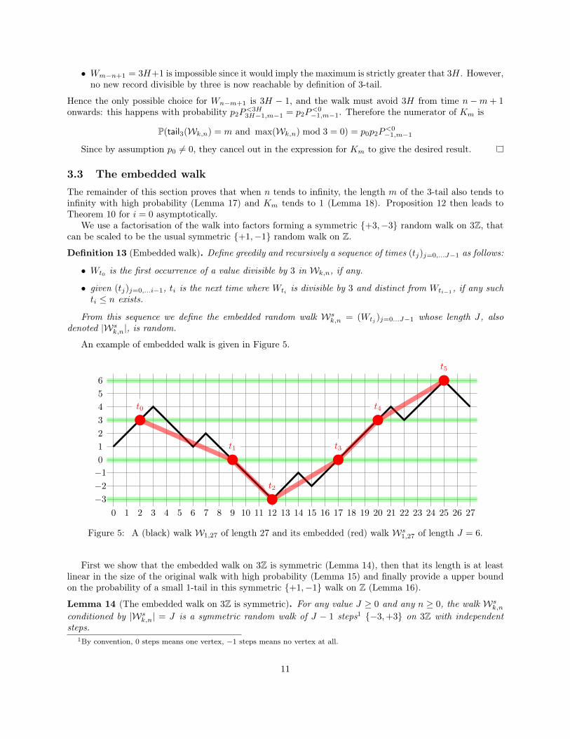
We consider an initial walk (black then red) from ti−1

to ti defined by the (Zt)t=ti−1+1,...ti = ( x )t∪ ( x )t.It defines a step +3 in the embedded walk. Themagenta interval starts at time si, which is the lastoccurrence of 0, and ends at time ti. In the magentainterval, τ transforms the (red) ( x )t into the (blue)( x )t.Observe that the blue part is up to translation thesymmetric of the red path via reflection with respectto a vertical axis and hence now defines a step from0 to −3 in the embedded walk.

0

1

2

1

0

2

0

1 1 1

2

1

2

0

2

1

2

1 1 1

0

ti−1 si ti

τ

Figure 6: Involution used in the proof of symmetry of the embedded walk

The following lemma ensures that the length of the embedded walk grows almost surely at least linearlyin n. This helps us later to convert bounds on 1-tail length in 1

3Wsk,n into bounds on 3-tail length in Wk,n.

Lemma 15 (The embedded walk’s length is almost always linear). There exists E > 0 and N ≥ 0, suchthat for any β ∈]0, 1/(16E)[ and n ≥ N we have

P(|Wsk,n| < βn) < C(β) exp(−D(β)n)

where C(β) and D(β) > 0 are non-negative functions of β made explicit in the proof.

Proof. Split the variables (Zi)i=1,...n used in the definition of the walk into independent factors of 4 variables((Z]4a,4(a+1)])a=0,...bn/4c. Now define variables (Xa)a=0,...bn/4c as follows:

Xa =

{1 if Z]4a,4(a+1)] ∈ {(0, 1, 2, 0), (0, 2, 1, 0)}0 otherwise .

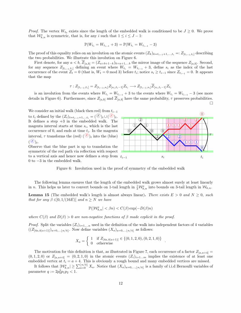
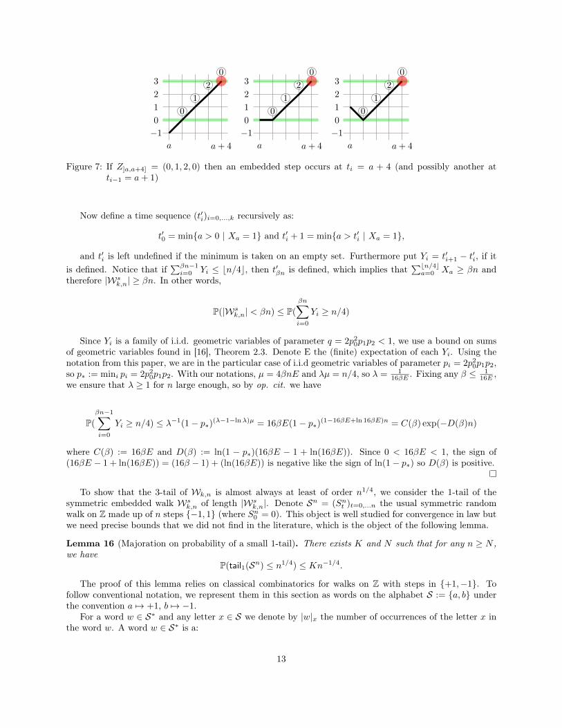
The motivation for this definition is that, as illustrated in Figure 7, each occurrence of a factor Z]a,a+4] =(0, 1, 2, 0) or Z]a,a+4] = (0, 2, 1, 0) in the atomic events (Zi)i=1...m implies the existence of at least oneembedded vertex at ti = a+ 4. This is obviously a rough bound and many embedded vertices are missed.

It follows that |Wsk,n| ≥

∑bn/4ca=0 Xa. Notice that (Xa)a=0,...,bn/4c is a family of i.i.d Bernoulli variables of

parameter q := 2p20p1p2 < 1.

12

−1

0

1

2

3

a a+ 4

0

1

2

0

−1

0

1

2

3

a a+ 4

0

1

2

0

−1

0

1

2

3

a a+ 4

0

1

2

0

Figure 7: If Z]a,a+4] = (0, 1, 2, 0) then an embedded step occurs at ti = a + 4 (and possibly another atti−1 = a+ 1)

Now define a time sequence (t′i)i=0,...,k recursively as:

t′0 = min{a > 0 | Xa = 1} and t′i + 1 = min{a > t′i | Xa = 1},

and t′i is left undefined if the minimum is taken on an empty set. Furthermore put Yi = t′i+1 − t′i, if itis defined. Notice that if

∑βn−1i=0 Yi ≤ bn/4c, then t′βn is defined, which implies that

∑bn/4ca=0 Xa ≥ βn and

therefore |Wsk,n| ≥ βn. In other words,

P(|Wsk,n| < βn) ≤ P(

βn∑i=0

Yi ≥ n/4)

Since Yi is a family of i.i.d. geometric variables of parameter q = 2p20p1p2 < 1, we use a bound on sumsof geometric variables found in [16], Theorem 2.3. Denote E the (finite) expectation of each Yi. Using thenotation from this paper, we are in the particular case of i.i.d geometric variables of parameter pi = 2p20p1p2,so p∗ := mini pi = 2p20p1p2. With our notations, µ = 4βnE and λµ = n/4, so λ = 1

16βE . Fixing any β ≤ 116E ,

we ensure that λ ≥ 1 for n large enough, so by op. cit. we have

P(

βn−1∑i=0

Yi ≥ n/4) ≤ λ−1(1− p∗)(λ−1−lnλ)µ = 16βE(1− p∗)(1−16βE+ln 16βE)n = C(β) exp(−D(β)n)

where C(β) := 16βE and D(β) := ln(1 − p∗)(16βE − 1 + ln(16βE)). Since 0 < 16βE < 1, the sign of(16βE − 1 + ln(16βE)) = (16β − 1) + (ln(16βE)) is negative like the sign of ln(1− p∗) so D(β) is positive.

To show that the 3-tail of Wk,n is almost always at least of order n1/4, we consider the 1-tail of thesymmetric embedded walk Ws

k,n of length |Wsk,n|. Denote Sn = (Snt )t=0,...n the usual symmetric random

walk on Z made up of n steps {−1, 1} (where Sn0 = 0). This object is well studied for convergence in law butwe need precise bounds that we did not find in the literature, which is the object of the following lemma.

Lemma 16 (Majoration on probability of a small 1-tail). There exists K and N such that for any n ≥ N ,we have

P(tail1(Sn) ≤ n1/4) ≤ Kn−1/4.

The proof of this lemma relies on classical combinatorics for walks on Z with steps in {+1,−1}. Tofollow conventional notation, we represent them in this section as words on the alphabet S := {a, b} underthe convention a 7→ +1, b 7→ −1.

For a word w ∈ S∗ and any letter x ∈ S we denote by |w|x the number of occurrences of the letter x inthe word w. A word w ∈ S∗ is a:

13

bridge if |w|a = |w|b. Bridges of length 2n are counted by central binomial coefficient(2nn

)= Θ(n−1/222n)

(and there are no bridges of odd length).

Dyck word if it is a bridge such that for any prefix p, |p|a ≥ |p|b. Dyck words of 2n letters are counted byCatalan numbers 1

2n+1

(2n+1n

)= Θ(n−3/222n).

meander if it is the prefix of a Dyck word. There is a classical folklore bijection2 between meanders of length2n and bridges of length 2n so meanders of even length 2n are also counted by

(2nn

)= Θ(n−1/222n).

We can deduce the number of meanders of odd length, say 2n+ 1, as follows. Decompose this meander intotwo parts: the prefix of length 2n, which is a meander; and the last letter. If the prefix is a Dyck word, thenthe last letter must be a; otherwise, it may be a or b. Hence the number of meanders of length 2n+ 1 is:

2

(2n

n

)− 1

2n+ 1

(2n+ 1

n

)= Θ(n−1/222n).

In a symmetric random walk, each letter a or b has the same independent probability 1/2. The probabilitythat any factor (Snt )t∈]`,`+k] of Sn is a meander is in Θ(k−1/2), while the probability that it is a Dyck word(assuming k is even) is in Θ(k−3/2).

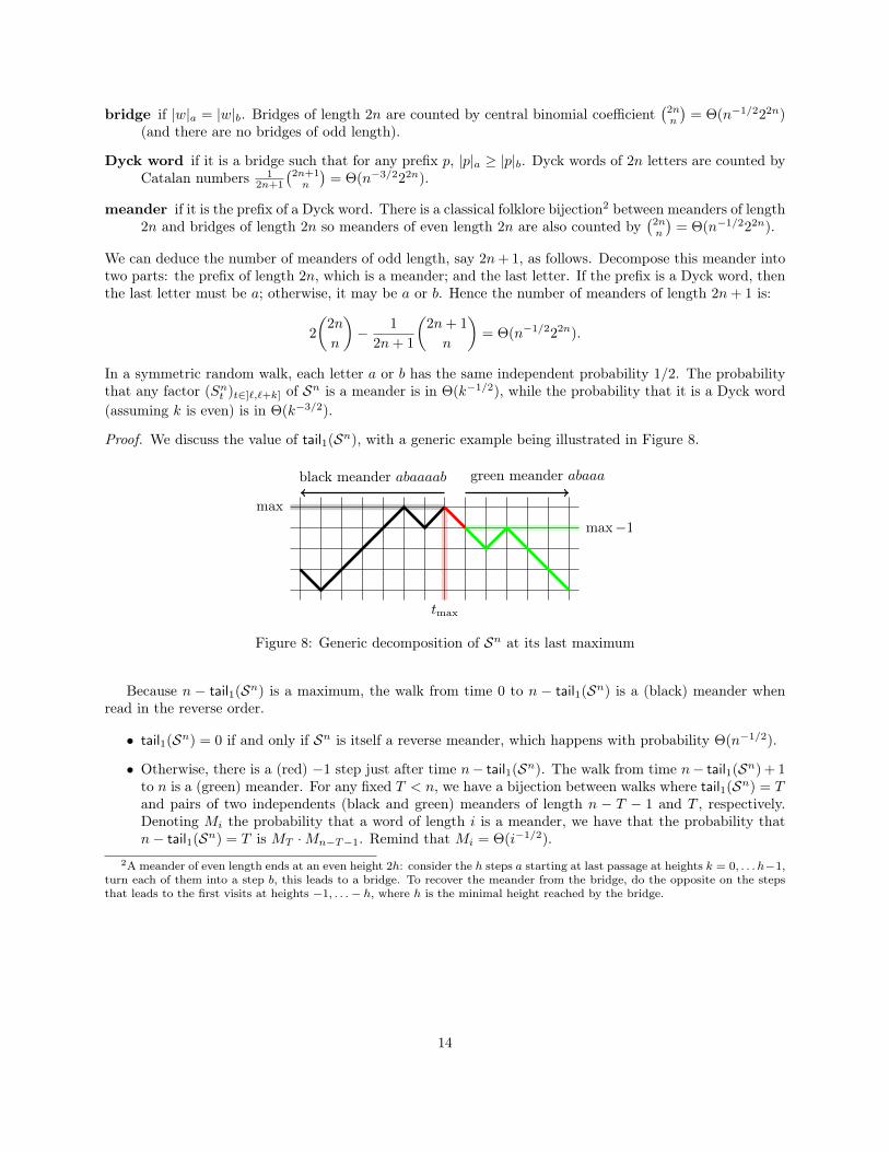
Proof. We discuss the value of tail1(Sn), with a generic example being illustrated in Figure 8.

max

black meander abaaaab

max−1

green meander abaaa

tmax

Figure 8: Generic decomposition of Sn at its last maximum

Because n − tail1(Sn) is a maximum, the walk from time 0 to n − tail1(Sn) is a (black) meander whenread in the reverse order.

• tail1(Sn) = 0 if and only if Sn is itself a reverse meander, which happens with probability Θ(n−1/2).

• Otherwise, there is a (red) −1 step just after time n− tail1(Sn). The walk from time n− tail1(Sn) + 1to n is a (green) meander. For any fixed T < n, we have a bijection between walks where tail1(Sn) = Tand pairs of two independents (black and green) meanders of length n − T − 1 and T , respectively.Denoting Mi the probability that a word of length i is a meander, we have that the probability thatn− tail1(Sn) = T is MT ·Mn−T−1. Remind that Mi = Θ(i−1/2).

2A meander of even length ends at an even height 2h: consider the h steps a starting at last passage at heights k = 0, . . . h−1,turn each of them into a step b, this leads to a bridge. To recover the meander from the bridge, do the opposite on the stepsthat leads to the first visits at heights −1, . . .− h, where h is the minimal height reached by the bridge.

14

Taking the two cases in consideration, it follows:

P(tail1(Sn) ≤ n1/4) ≤ P(tail1(Sn) = 0) +

n1/4∑T=1

P(tail1(Sn) = T )

≤Mn +

n1/4∑T=1

MTMn−T−1

≤ Θ(n−1/2) + n1/4 ·Θ(n−1/2)

≤ Θ(n−1/4),

where on the third line we used the fact that Mn−T−1 = Θ(n−1/2) and MT ≤ 1.Hence we have proved the lemma.

3.4 Back to the main walk, and end of the proofWe now transfer the bound on the probability of a small 1-tail for the symmetric embedded walk, obtainedin Lemma 16, to a similar upper bound for the 3-tail on the initial walk, using the probabilistic lower boundon the length of the embedded walk obtained in Lemma 15.

Lemma 17 (Upper bound for the probability of a small 3-tail). ∃γ, δ,N such that ∀n ≥ N ,

P(tail3(Wk,n) ≤ γn1/4) ≤ δn−1/4.

Proof. Let β a constant such that 0 < β < 1/E where E ≥ 1 is the expectation of each variable (Yi)i>0,defined in the proof of Lemma 15. We distinguish the cases where the embedded symmetric walk Ws

k,n hasmore or less than βn steps:

P(tail3(Wk,n) ≤ γn1/4) =P(tail3(Wk,n) ≤ γn1/4 | |Wsk,n| < βn) · P(|Ws

k,n| < βn)

+ P(tail3(Wk,n) ≤ γn1/4 | |Wsk,n| ≥ βn) · P(|Ws

k,n| ≥ βn)

For the first term, Lemma 15 ensures that the embedded walk has at least linear length with highprobability:

P(|Wsk,n| < βn) ≤ C(β) exp(−D(β)n).

For the second term, we use the (very rough) inclusion of events

tail3(Wk,n) ≤ γn1/4 =⇒ tail1(Wsk,n) ≤ γn1/4.

By Lemma 16, and fixing γ = β1/4, the 1-tail is small with low probability:

P(tail1(Wsk,n) ≤ γn1/4 | |Ws

k,n| ≥ βn) ≤ K(βn)−1/4

Summing both contributions, and bounding the other expressions by 1,

P(tail3(Wk,n) ≤ γn1/4) ≤ C(β) exp(−D(β)n) +K(βn)−1/4.

For n larger than an appropriate N , we have the constant δ allowing to bound this probability by δn−1/4as expected.

Remember that Km :=P<0−1,m−1

P<0−1,m

, where P<Hk,n is the probability that a random walk starting from k

remains strictly below H during n steps.

15

Lemma 18 (Bounds for Km). ∃α,M such that ∀m ≥M , 1 ≤ Km ≤ 1 + αm .

Proof. Reformulation of Km and lower bound 1. Let Em be the event:

W−1,m ∈ Em ⇔Wt < 0 for 0 ≤ t < m, and Wm = 0.

Among the walks that remains strictly below 0 for m− 1 steps, the event Em exactly excludes those thatremain strictly below 0 at the m-th step, so

P(Em) = P<0−1,m−1 − P<0

−1,m.

Dividing the previous equation by P<0−1,m we obtain that

Km = 1 +P(Em)

P<0−1,m−1

.

The lower bound 1 ≤ Km follows.

Upper bound on Km We now find an upper bound on the numerator P(Em).First condition the event Em by the possible length ` of the embedded walk:

P(Em) =

+∞∑`=0

P(Em and |Ws−1,m| = `).

Fix β such that 0 < β < 1/E, and consider the terms such that ` < βm. By Lemma 15, we have:

βm−1∑`=0

P(Em and |Ws−1,m| = `) ≤ P(|Ws

−1,m| < βm) ≤ C(β) exp(−D(β)m)

We now consider the remaining terms (` ≥ βm). First translate the event Em on the embedded symmetricwalkWs

−1,m. Define the flip as the morphism {a, b}∗ → {a, b}∗ exchanging letters a and b. On the one hand,we have:

W−1,m ∈ Em and |Ws−1,m| = ` ⇐⇒ Ws

−1,m is a flipped Dyck word of `− 2 steps followed by a +1 step

since the first value divisible by 3 is −3 and the first non-negative value divisible by 3 is Wm = 0 thatcorresponds to the end of Ws

−1,m.On the other hand,

W−1,m−1 ∈W<0−1,m−1 and |Ws

−1,m−1| = ` ⇐⇒ Ws−1,m is a flipped meander of `− 1 steps

since avoiding 0 in W−1,m−1 is by definition equivalent to the fact that Ws−1,m−1 (starting in −3) never visit

0.Since the walk Ws

−1,m is symmetric, we can use classical combinatorics giving 1/2 probability to eachstep to estimate the conditional probabilities:

P(Em | |Ws−1,m| = `) = 2−(`−1)|number of Dyck words of `− 2 steps|

since the last step must be a +1 and

P(W<0−1,m−1 | |Ws

−1,m−1| = `) = 2−(`−1)|number of meanders of `− 1 steps|.

From the counting formula of Dyck words and meanders we get a classical result in combinatorics:

|number of Dyck words of `− 2 steps||number of meanders of `− 1 steps|

=

{1

2`−3 if ` = 0 mod 2

0 otherwise

16

We turn this equality into a uniform upper bound using the assumption ` ≥ βm.

2−(`−1)|number of Dyck words of `− 2 steps|2−(`−1)|number of meanders of `− 1 steps|

≤ 1

2`− 3≤ 1

2βm− 3.

Summing up, we have

∑`≥βm

P(Em | |Ws−1,m| = `) · P(|Ws

−1,m| = `) ≤ 1

2βm− 3

∑`≥βm

P(W<0−1,m−1 | |Ws

−1,m−1| = `) · P(|Ws−1,m−1| = `)

≤ 1

2βm− 3P<0−1,m−1,

and therefore, adding the missing terms for ` < βm:

P(Em) ≤ C(β) exp (−D(β)m) +1

2βm− 3P<0−1,m−1.

Now fix any α < 12β , and we get for m large enough the expected bound:

P(Em) ≤ α

mP<0−1,m−1.

From the decomposition of Km we deduce that for m ≥M ,

Km ≤ 1 +α

m.

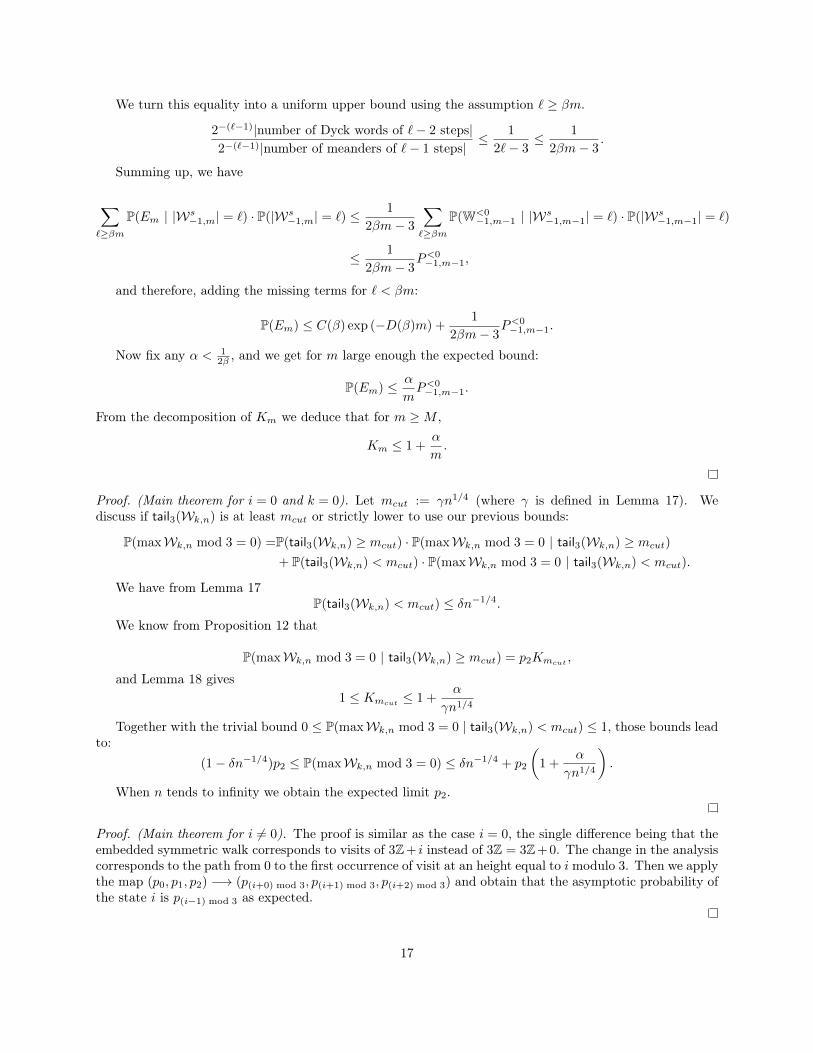
Proof. (Main theorem for i = 0 and k = 0). Let mcut := γn1/4 (where γ is defined in Lemma 17). Wediscuss if tail3(Wk,n) is at least mcut or strictly lower to use our previous bounds:

P(maxWk,n mod 3 = 0) =P(tail3(Wk,n) ≥ mcut) · P(maxWk,n mod 3 = 0 | tail3(Wk,n) ≥ mcut)

+ P(tail3(Wk,n) < mcut) · P(maxWk,n mod 3 = 0 | tail3(Wk,n) < mcut).

We have from Lemma 17P(tail3(Wk,n) < mcut) ≤ δn−1/4.

We know from Proposition 12 that

P(maxWk,n mod 3 = 0 | tail3(Wk,n) ≥ mcut) = p2Kmcut,

and Lemma 18 gives1 ≤ Kmcut ≤ 1 +

α

γn1/4

Together with the trivial bound 0 ≤ P(maxWk,n mod 3 = 0 | tail3(Wk,n) < mcut) ≤ 1, those bounds leadto:

(1− δn−1/4)p2 ≤ P(maxWk,n mod 3 = 0) ≤ δn−1/4 + p2

(1 +

α

γn1/4

).

When n tends to infinity we obtain the expected limit p2.

Proof. (Main theorem for i 6= 0). The proof is similar as the case i = 0, the single difference being that theembedded symmetric walk corresponds to visits of 3Z+ i instead of 3Z = 3Z+ 0. The change in the analysiscorresponds to the path from 0 to the first occurrence of visit at an height equal to imodulo 3. Then we applythe map (p0, p1, p2) −→ (p(i+0) mod 3, p(i+1) mod 3, p(i+2) mod 3) and obtain that the asymptotic probability ofthe state i is p(i−1) mod 3 as expected.

17

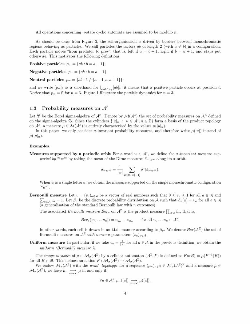
4 ConclusionOther models It is natural to ask whether a similar phenomenon occurs in more complex models of cyclicdominance.

The easiest extension is to consider that each predator has a fixed probability p < 1 to replace its prey(probabilistic version). Although the global behaviour seems similar (see Figure 9), the probability that asmall region surrounded by a predator and a prey disappears may impact the early dynamics; noise has beenshown to create the possibility of this kind of “unlucky extinctions” in non-spatial models [23]. Experimentalevidence seems to indicate a much slower convergence and no obvious numerical relationship between theinitial parameters and asymptotic probability.

In higher dimension, we are so far from a complete understanding of the dynamics and limit measure [7]that no conjecture seems possible.

We believe that the random walk approach (Proposition 9) can be adapted to more general prey/predatorrelationship. Consider the prey/predator graph, where the oriented edge i → j means that i is a predatorfor j. Beyond the simple 3-state cyclic dominance, more complex predator/prey graphs have been observedin nature [30, 28, 22]. As a first example, we believe Proposition 9 holds on alphabets of size 2k + 1 whereeach state n has k predators n+ 1, n+ 2, . . . n+ k and k preys n− 1, . . . n− k (modulo 2k+ 1). The randomwalk has steps in {−k,+k}, with the same condition that W [x]i must be equal to xi modulo 2k + 1.

The clearest limit to our approach is the presence of neutral particles, which can interact with otherparticles in ways that we cannot seem to describe in terms of a simple height function (as an example, inthe 4-state cyclic cellular automaton, a neutral particle can turn a positive particle into a negative particle,or the opposite). The absence of neutral particle means that the prey/predator relationship corresponds toan orientation of the complete graph (a tournament).

Max path preservation We believe that a necessary and sufficient condition for Proposition 9 to hold isthe following. Assume the alphabet is Z/nZ and denote a < b < c if, by incrementing a by one repeatedly,one reaches b before c. A complete graph orientation is max path preserving if, for any triplet of distinctvertices/species a < b < c, if a and b are predators for c, (a → c and b → c) then b is a predator for a(b→ a).

The definition of the walk W [x] becomes the following:

• w0 = x0

• if xi = xi+1 then wi+1 = wi

• if xi is a prey for xi+1 then wi+1 is the value equal to xi+1 modulo n in {xi + 1, . . . xi + n− 1}

• if xi is a predator for xi+1 then wi+1 is the value equal to xi+1 modulo n in {xi − 1, . . . xi − (n− 1)}.

To understand the max path preserving assumption, consider the following situation: a factor xixi+1xi+2 =acb such that a < b < c and a and b are predators for c. We have W [x]i > W [x]i+1 < W [x]i+2 and, sincea < b < c, W [x]i < W [x]i+2. Since this factor becomes ab at the next time step and the walk steps up, wewant b to predate a.

Brute force enumeration up to n = 6 suggests three families of prey-predator graphs for n species withthe max-path preserving property:

• the n total orders compatible with the cyclic increments: k, k− 1, . . . 0, n− 1, n− 2, . . . k+ 1 for k from0 to n− 1 (the corresponding cellular automata is uninteresting as k− 1 dominates every other state).

• some strongly connected prey/predator graphs where 0, n−1, n−2, . . . 1, 0 forms an Hamiltonian cycle.

• some strongly connected prey/predator graphs where 0, n−1, n−2, . . . 1, 0 is not an Hamiltonian cycle(but there is at least one Hamiltonian cycle, like for any strongly connected tournament).

18

The smallest example of the third family corresponds to the 3-state cyclic automaton where prey/predatorrelations between distinct species are reversed. Notice that the resulting walk on Z consists of steps ±2instead of steps ±1. Of course we could consider the minimum on the walk on steps ±1 instead, but we donot know if relabelling the prey/predator graphs of the third family according to one of the possibly manyHamiltonian cycles leads to a structure similar to the second family in general.

Up to n = 6, the last two families are counted by the Eulerian numbers (A000295 in OEIS):

en :=

b(n−1)/2c∑k=1

(n

2k + 1

).

We conjecture the following characterisation: any orientation in the second family is defined by selectingan odd number of vertices 0 ≤ c1 < c2 < · · · < c2k+1 ≤ n − 1, where 3 ≤ 2k + 1 ≤ n and the ordercorresponds to the numerotation in the hamiltonian cycle 0, n− 1, n− 2, . . . 1, 0. The convention is that forany state j in the cyclic interval ]ci, ci+1], j is a predator for any state in [ci−k mod 2k+1, j[. Since the numberof possible cycles of 2k+ 1 vertices is counted by the binomial coefficient

(n

2k+1

), this characterisation would

imply the counting above. Empirically, all orientations defined by this conjectural characterisation satisfythe max path preservation up to n = 11 species.

If Proposition 9 does generalise to these three graph families, it remains to check that the rest of theproof does as well. We expect a more systematic analysis using functional equations.

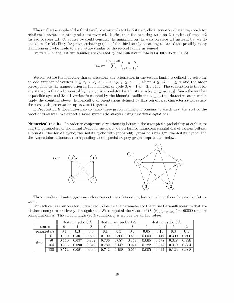
Numerical results In order to conjecture a relationship between the asymptotic probability of each stateand the parameters of the initial Bernoulli measure, we performed numerical simulations of various cellularautomata: the 3-state cyclic; the 3-state cyclic with probability (invasion rate) 1/2; the 4-state cyclic; andthe two cellular automata corresponding to the predator/prey graphs represented below.

0 1

23

G1 :

0

1

23

4

G2 :

These results did not suggest any clear conjectural relationship, but we include them for possible futurework.

For each cellular automaton F , we fixed values for the parameters of the initial Bernoulli measure that aredistinct enough to be clearly distinguished. We computed the values of (F t(x)0)0≤t≤150 for 100000 randomconfigurations x. The error margin (95% confidence) is ±0.002 for all the values.

3-state cyclic CA 3-state w/ proba 1/2 4-state cyclic CAstates 0 1 2 0 1 2 0 1 2 3

parameters 0.1 0.3 0.6 0.1 0.3 0.6 0.05 0.15 0.3 0.5

time

0 0.100 0.301 0.599 0.100 0.300 0.600 0.050 0.149 0.300 0.50050 0.550 0.087 0.362 0.760 0.087 0.153 0.065 0.578 0.018 0.339100 0.565 0.090 0.345 0.780 0.147 0.074 0.122 0.615 0.019 0.354150 0.572 0.091 0.336 0.742 0.198 0.060 0.005 0.615 0.123 0.368

19

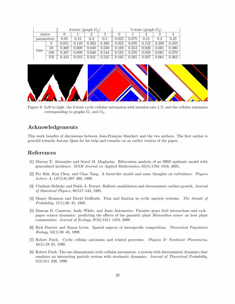
4-state (graph G1) 5-state (graph G2)states 0 1 2 3 0 1 2 3 4

parameters 0.05 0.15 0.3 0.5 0.025 0.075 0.15 0.3 0.45

time

0 0.051 0.149 0.302 0.498 0.025 0.076 0.152 0.298 0.45050 0.369 0.009 0.040 0.580 0.169 0.354 0.026 0.061 0.390100 0.407 0.009 0.040 0.544 0.165 0.376 0.028 0.061 0.370150 0.424 0.010 0.041 0.525 0.165 0.385 0.027 0.061 0.362

Figure 9: Left to right, the 3-state cyclic cellular automaton with invasion rate 1/2, and the cellular automatacorresponding to graphs G1 and G2.

AcknowledgementsThis work benefits of discussions between Jean-François Marckert and the two authors. The first author isgrateful towards Antony Quas for his help and remarks on an earlier version of the paper.

References[1] Murray E. Alexander and Seyed M. Moghadas. Bifurcation analysis of an SIRS epidemic model with

generalized incidence. SIAM Journal on Applied Mathematics, 65(5):1794–1816, 2005.

[2] Per Bak, Kan Chen, and Chao Tang. A forest-fire model and some thoughts on turbulence. PhysicsLetters A, 147(5-6):297–300, 1990.

[3] Vladimir Belitsky and Pablo A. Ferrari. Ballistic annihilation and deterministic surface growth. Journalof Statistical Physics, 80:517–543, 1995.

[4] Maury Bramson and David Griffeath. Flux and fixation in cyclic particle systems. The Annals ofProbability, 17(1):26–45, 1989.

[5] Duncan D. Cameron, Andy White, and Janis Antonovics. Parasite–grass–forb interactions and rock–paper–scissor dynamics: predicting the effects of the parasitic plant Rhinanthus minor on host plantcommunities. Journal of Ecology, 97(6):1311–1319, 2009.

[6] Rick Durrett and Simon Levin. Spatial aspects of interspecific competition. Theoretical PopulationBiology, 53(1):30–43, 1998.

[7] Robert Fisch. Cyclic cellular automata and related processes. Physica D: Nonlinear Phenomena,45(1):19–25, 1990.

[8] Robert Fisch. The one-dimensional cyclic cellular automaton: a system with deterministic dynamics thatemulates an interacting particle system with stochastic dynamics. Journal of Theoretical Probability,3(2):311–338, 1990.

20

[9] Robert Fisch. Clustering in the one-dimensional three-color cyclic cellular automaton. The Annals ofProbability, 20:1528–1548, 1992.

[10] Eric Foxall and Hanbaek Lyu. Clustering in the three and four color cyclic particle systems in onedimension. Journal of Statistical Physics, 171(3):1–14, 2018.

[11] Marcus Frean and Edward R. Abraham. Rock–scissors–paper and the survival of the weakest. Proceed-ings of the Royal Society of London. Series B: Biological Sciences, 268(1474):1323–1327, 2001.

[12] Christian Guill, Barbara Drossel, Wolfram Just, and Eddy Carmack. A three-species model explainingcyclic dominance of Pacific salmon. Journal of Theoretical Biology, 276(1):16–21, 2011.

[13] Christoph Hauert, Silvia De Monte, Josef Hofbauer, and Karl Sigmund. Volunteering as Red Queenmechanism for cooperation in public goods games. Science, 296(5570):1129–1132, 2002.

[14] Benjamin Hellouin de Menibus and Mathieu Sablik. Self-organisation in cellular automata with coales-cent particles: qualitative and quantitative approaches. Journal of Statistical Physics, 167(5):1180–1220,2017.

[15] Lorens A. Imhof, Drew Fudenberg, and Martin A. Nowak. Evolutionary cycles of cooperation anddefection. Proceedings of the National Academy of Sciences, 102(31):10797–10800, 2005.

[16] Svante Janson. Tail bounds for sums of geometric and exponential variables. Statistics & ProbabilityLetters, 135:1–6, 2018.

[17] Benjamin Kerr, Margaret A. Riley, Marcus W. Feldman, and Brendan J. M. Bohannan. Local dispersalpromotes biodiversity in a real-life game of rock–paper–scissors. Nature, 418(6894):171, 2002.

[18] Benjamin C. Kirkup and Margaret A. Riley. Antibiotic-mediated antagonism leads to a bacterial gameof rock–paper–scissors in vivo. Nature, 428(6981):412, 2004.

[19] Benoit Laslier, Jean-François Laslier, et al. Reinforcement learning from comparisons: Three alternativesare enough, two are not. The Annals of Applied Probability, 27(5):2907–2925, 2017.

[20] Hanbaek Lyu and David Sivakoff. Persistence of sums of correlated increments and clustering in cellularautomata. Stochastic Processes and their Applications, 2018.

[21] Robert M. May and Warren J. Leonard. Nonlinear aspects of competition between three species. SIAMJournal on Applied Mathematics, 29(2):243–253, 1975.

[22] Daniel S. Maynard, Mark A. Bradford, Daniel L. Lindner, Linda T. A. van Diepen, Serita D. Frey,Jessie A. Glaeser, and Thomas W. Crowther. Diversity begets diversity in competition for space.Nature ecology & evolution, 1(6):0156, 2017.

[23] Tobias Reichenbach, Mauro Mobilia, and Erwin Frey. Coexistence versus extinction in the stochasticcyclic Lotka-Volterra model. Physical Review E, 74(5):051907, 2006.

[24] Dirk Semmann, Hans-Jürgen Krambeck, and Manfred Milinski. Volunteering leads to rock–paper–scissors dynamics in a public goods game. Nature, 425(6956):390, 2003.

[25] Cosma Rohilla Shalizi and Kristina Lisa Shalizi. Quantifying self-organization in cyclic cellular au-tomata. In Noise in Complex Systems and Stochastic Dynamics, volume 5114, pages 108–118. Interna-tional Society for Optics and Photonics, 2003.

[26] Karl Sigmund. Oscillations in the evolution of reciprocity. Journal of Theoretical Biology, 137:21–26,1989.

21

[27] Barry Sinervo and Curt M. Lively. The rock–paper–scissors game and the evolution of alternative malestrategies. Nature, 380(6571):240, 1996.

[28] György Szabó and Tamás Czárán. Phase transition in a spatial Lotka-Volterra model. Physical ReviewE, 63(6):061904, 2001.

[29] György Szabó and Gabor Fath. Evolutionary games on graphs. Physics Reports, 446(4-6):97–216, 2007.

[30] Attila Szolnoki, Mauro Mobilia, Luo-Luo Jiang, Bartosz Szczesny, Alastair M. Rucklidge, and MatjažPerc. Cyclic dominance in evolutionary games: a review. Journal of the Royal Society Interface,11(100):20140735, 2014.

[31] Kei-ichi Tainaka. Lattice model for the Lotka-Volterra system. Journal of the Physical Society of Japan,57(8):2588–2590, 1988.

[32] Kei-ichi Tainaka. Paradoxical effect in a three-candidate voter model. Physics Letters A, 176(5):303–306,1993.

22