Behavior Progress Monitoring

Tools and Strategies Using ExcelCathy Jensen

cjensen@ttsd.k12.or.us

Jensen, April 2014

Types of Data

Combined reinforcement / data:•Daily Percentages•Green / Yellow / Red

Data only:•Health and Behavior Monitoring

Jensen, April 2014

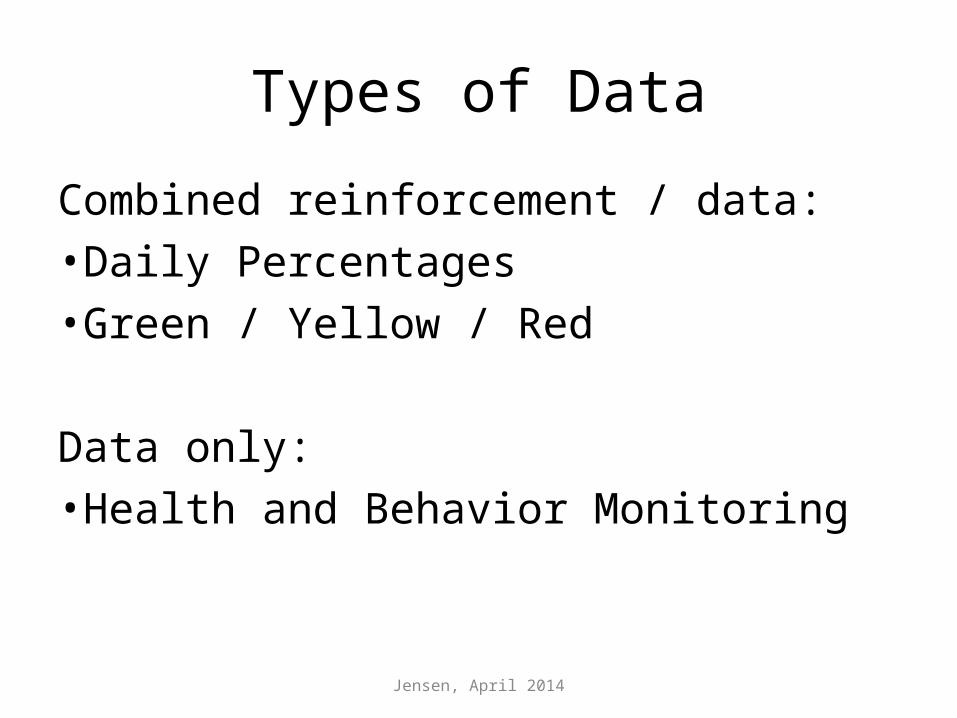
Daily Percentage:Elementary

Daily Goal: 70% totalAs the student experiences success, increase the goal to 80-85%.

Jensen, April 2014

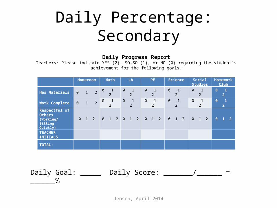
Daily Percentage: Secondary

  Homeroom Math LA PE Science Social Studies

Homework Club

Has Materials 0 1 2 0 1 2 0 1 2 0 1 2 0 1 2 0 1 2 0   1   2

Work Complete 0 1 2 0 1 2 0 1 2 0 1 2 0 1 2 0 1 2 0   1   2

Respectful of Others(Working/Sitting Quietly)

0 1 2 0 1 2 0 1 2 0 1 2 0 1 2 0 1 2 0  1  2

TEACHER INITIALS

 

TOTAL:     

       

Daily Progress ReportTeachers: Please indicate YES (2), SO-SO (1), or NO (0) regarding the student’s achievement

for the following goals.

Daily Goal: _____ Daily Score: _______/______ = ______%

Jensen, April 2014

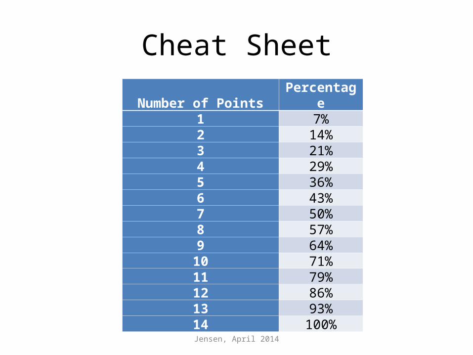
Cheat SheetNumber of Points Percentage

1 7%2 14%3 21%4 29%5 36%6 43%7 50%8 57%9 64%10 71%11 79%12 86%13 93%14 100%

Jensen, April 2014

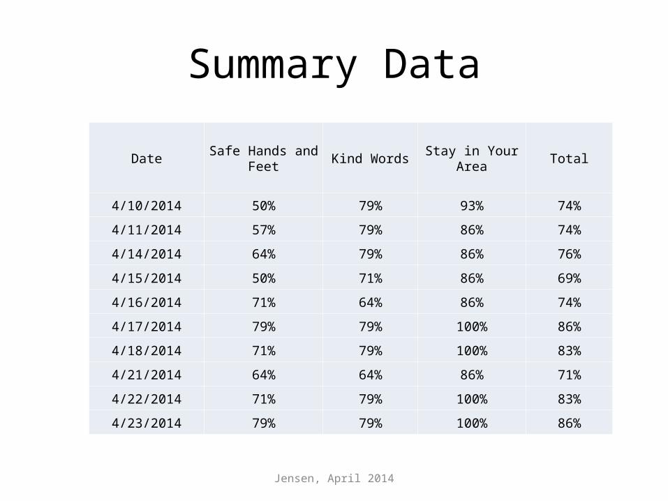
Summary Data

Date Safe Hands and Feet Kind Words Stay in Your Area Total

4/10/2014 50% 79% 93% 74%

4/11/2014 57% 79% 86% 74%

4/14/2014 64% 79% 86% 76%

4/15/2014 50% 71% 86% 69%

4/16/2014 71% 64% 86% 74%

4/17/2014 79% 79% 100% 86%

4/18/2014 71% 79% 100% 83%

4/21/2014 64% 64% 86% 71%

4/22/2014 71% 79% 100% 83%

4/23/2014 79% 79% 100% 86%

Jensen, April 2014

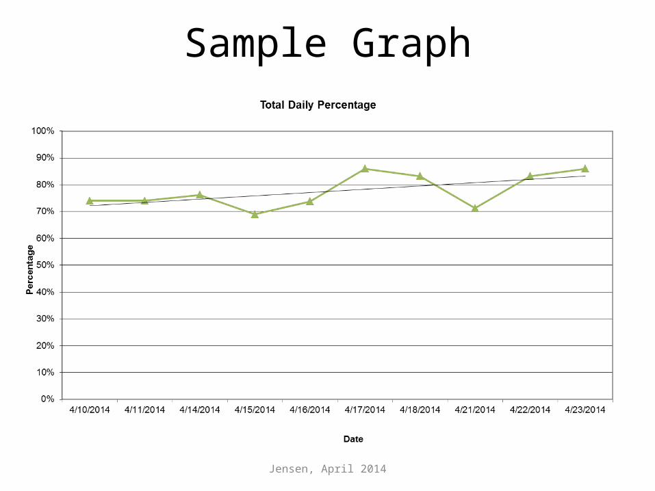
Sample Graph

Jensen, April 2014

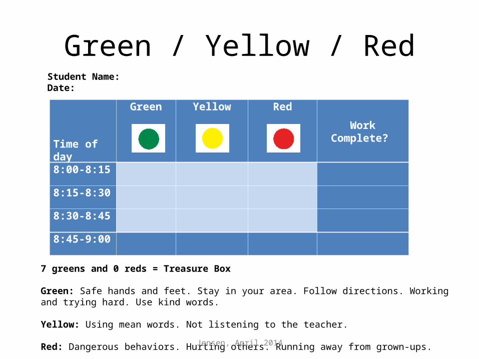
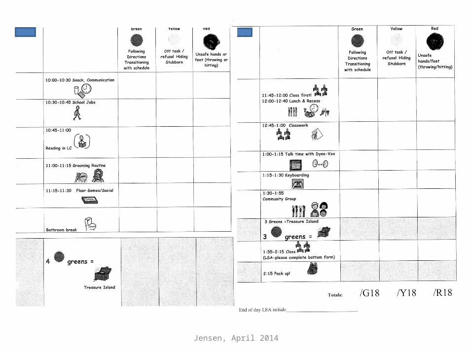
Green / Yellow / RedStudent Name:Date:

7 greens and 0 reds = Treasure Box

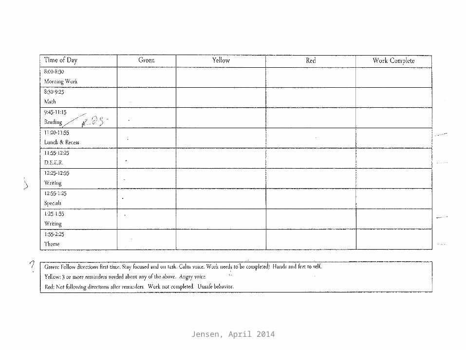
Green: Safe hands and feet. Stay in your area. Follow directions. Working and trying hard. Use kind words.

Yellow: Using mean words. Not listening to the teacher.

Red: Dangerous behaviors. Hurting others. Running away from grown-ups.

Time of day

Green  

Yellow  

Red   Work Complete? 

8:00-8:15  

8:15-8:30  

8:30-8:45  

8:45-9:00        

Jensen, April 2014

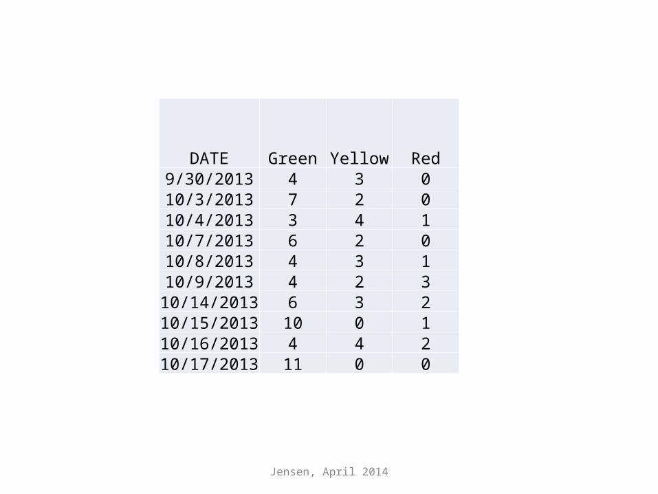
DATE Green Yellow Red9/30/2013 4 3 010/3/2013 7 2 010/4/2013 3 4 110/7/2013 6 2 010/8/2013 4 3 110/9/2013 4 2 3

10/14/2013 6 3 210/15/2013 10 0 110/16/2013 4 4 210/17/2013 11 0 0

Jensen, April 2014

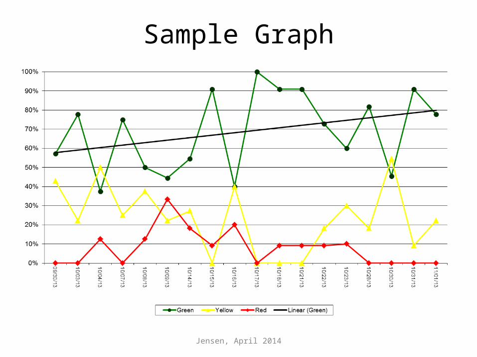
Sample Graph

Jensen, April 2014

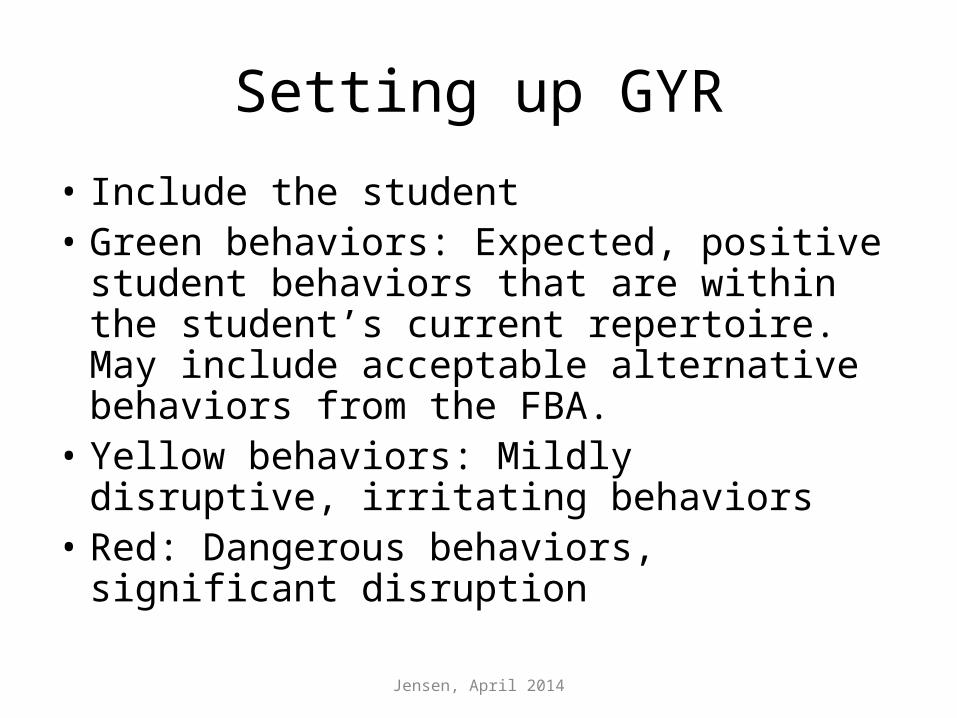
Setting up GYR

• Include the student• Green behaviors: Expected, positive student

behaviors that are within the student’s current repertoire. May include acceptable alternative behaviors from the FBA.

• Yellow behaviors: Mildly disruptive, irritating behaviors

• Red: Dangerous behaviors, significant disruption

Jensen, April 2014

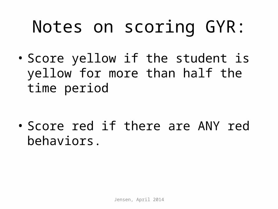
Notes on scoring GYR:

• Score yellow if the student is yellow for more than half the time period

• Score red if there are ANY red behaviors.

Jensen, April 2014

Health and Behavior Tracking

• Not seen by the student• The form gives a daily graph that reflects the

changes and patterns of behaviors

Jensen, April 2014

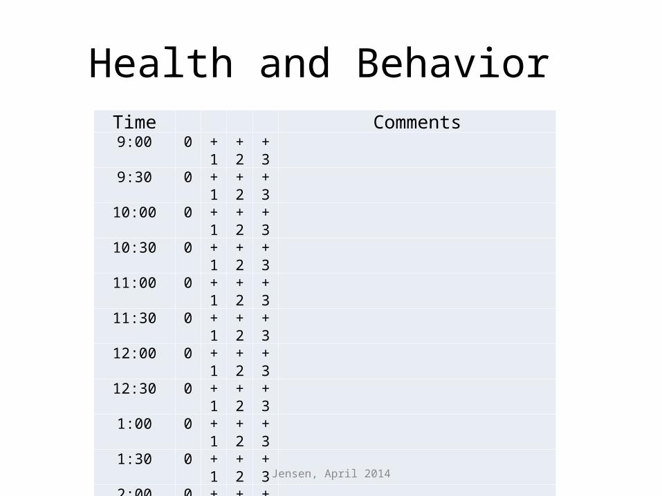
Health and Behavior Time Comments9:00 0 +1 +2 +3

9:30 0 +1 +2 +3

10:00 0 +1 +2 +3

10:30 0 +1 +2 +3

11:00 0 +1 +2 +3

11:30 0 +1 +2 +3

12:00 0 +1 +2 +3

12:30 0 +1 +2 +3

1:00 0 +1 +2 +3

1:30 0 +1 +2 +3

2:00 0 +1 +2 +3

2:30 0 +1 +2 +3

Jensen, April 2014

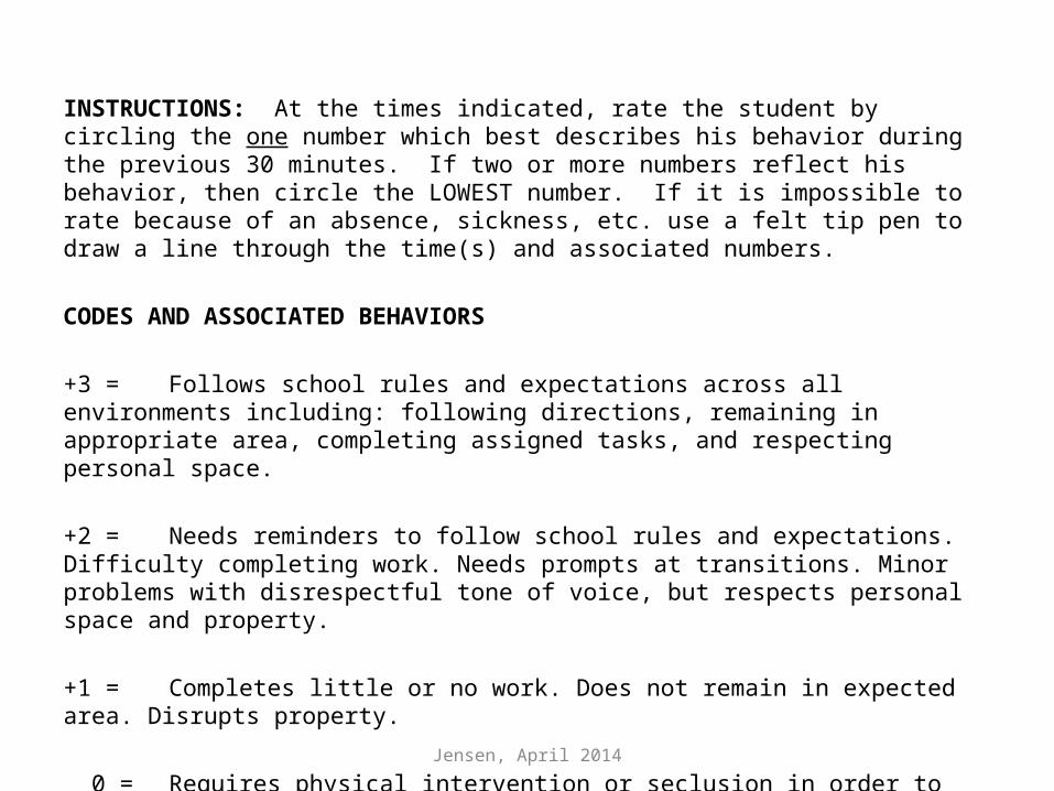
INSTRUCTIONS: At the times indicated, rate the student by circling the one number which best describes his behavior during the previous 30 minutes. If two or more numbers reflect his behavior, then circle the LOWEST number. If it is impossible to rate because of an absence, sickness, etc. use a felt tip pen to draw a line through the time(s) and associated numbers. CODES AND ASSOCIATED BEHAVIORS +3 = Follows school rules and expectations across all environments including: following directions, remaining in appropriate area, completing assigned tasks, and respecting personal space. +2 = Needs reminders to follow school rules and expectations. Difficulty completing work. Needs prompts at transitions. Minor problems with disrespectful tone of voice, but respects personal space and property. +1 = Completes little or no work. Does not remain in expected area. Disrupts property. 0 = Requires physical intervention or seclusion in order to remain safe. Makes verbal threats to peers or staff. Aggressive personal space violations.

Jensen, April 2014

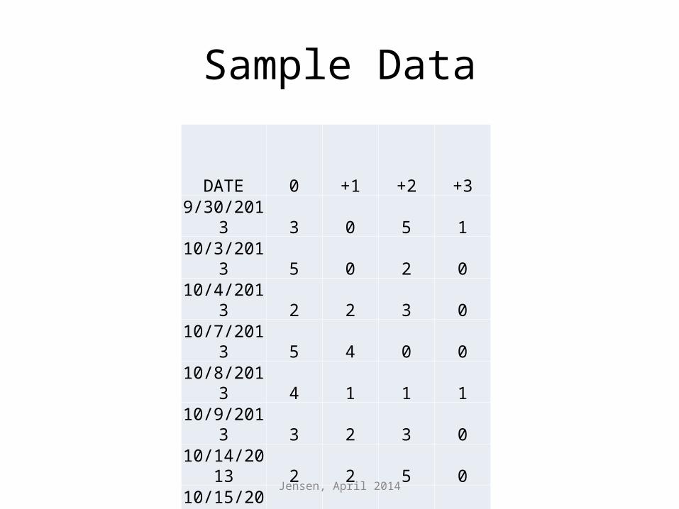
Sample Data

DATE 0 +1 +2 +39/30/2013 3 0 5 110/3/2013 5 0 2 010/4/2013 2 2 3 010/7/2013 5 4 0 010/8/2013 4 1 1 110/9/2013 3 2 3 0

10/14/2013 2 2 5 010/15/2013 3 2 3 010/16/2013 4 2 3 010/17/2013 3 2 3 0

Jensen, April 2014

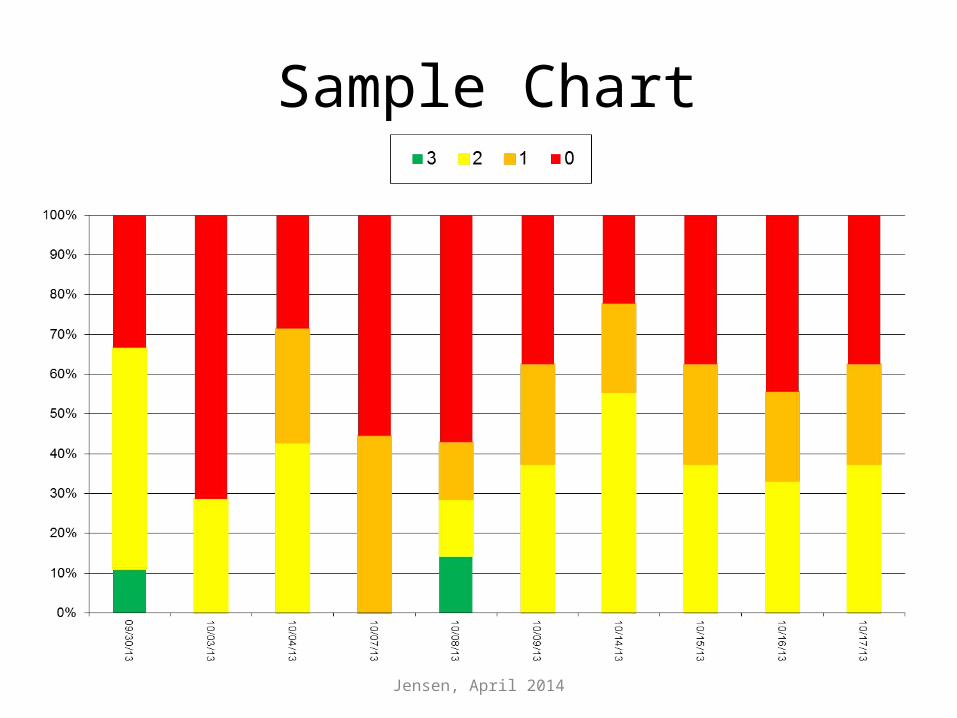
Sample Chart

Jensen, April 2014

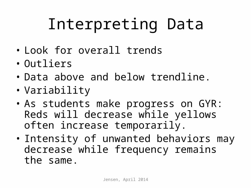
Interpreting Data

• Look for overall trends• Outliers• Data above and below trendline.• Variability• As students make progress on GYR: Reds will

decrease while yellows often increase temporarily.

• Intensity of unwanted behaviors may decrease while frequency remains the same.

Jensen, April 2014

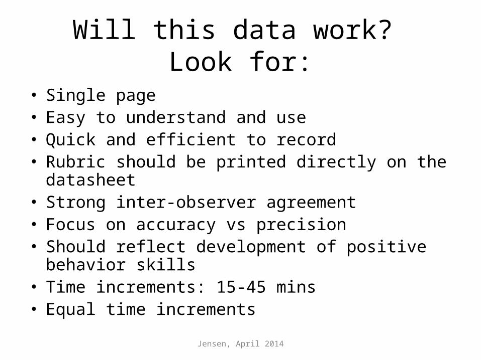
Will this data work? Look for:

• Single page• Easy to understand and use• Quick and efficient to record• Rubric should be printed directly on the datasheet• Strong inter-observer agreement• Focus on accuracy vs precision• Should reflect development of positive behavior skills• Time increments: 15-45 mins• Equal time increments

Jensen, April 2014

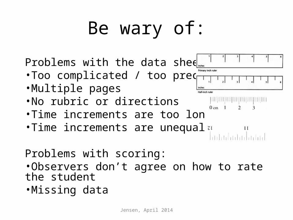
Be wary of:

Problems with the data sheet format:•Too complicated / too precise•Multiple pages•No rubric or directions•Time increments are too long•Time increments are unequal

Problems with scoring:•Observers don’t agree on how to rate the student•Missing data

Jensen, April 2014

System over-represents negative behaviors:•Behavior goals stated in the negative (i.e. “No yelling.”)•Response cost systems•“Poisoned Cues” – data system is used punitively

Problems with types of data:•Tallies

Jensen, April 2014

Jensen, April 2014

Jensen, April 2014

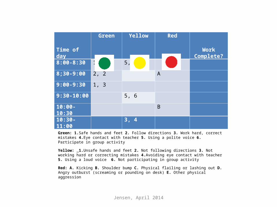
Time of day

Green  

Yellow  

Red   Work 

Complete?8:00-8:30 1, 2 5, 3  

8;30-9:00 2, 2 A  

9:00-9:30 1, 3  

9:30-10:00 5, 6  

10:00-10:30 B  

10:30-11:00   3, 4    

Green: 1.Safe hands and feet 2. Follow directions 3. Work hard, correct mistakes 4.Eye contact with teacher 5. Using a polite voice 6. Participate in group activity

Yellow: 1.Unsafe hands and feet 2. Not following directions 3. Not working hard or correcting mistakes 4.Avoiding eye contact with teacher 5. Using a loud voice 6. Not participating in group activity

Red: A. Kicking B. Shoulder bump C. Physical flailing or lashing out D. Angry outburst (screaming or pounding on desk) E. Other physical aggression

Jensen, April 2014

People will complain about…

• Lack of precision• Doesn’t indicate intensity• Not punitive enough• “I told him if he didn’t stop running he would

get a red, and he ran away anyway.”• Kids escalate when they earn red

Jensen, April 2014

Keep in mind…

• Data is for the stakeholders and should only be used in context – i.e. not the only type of data used for placement

• The system can be adjusted to meet the needs of the team

• Looking for patterns, progress• Reinforcement vs. motivation• A pointcard should be a tool for providing

positive feedback.

Jensen, April 2014

Using Excel

Jensen, April 2014

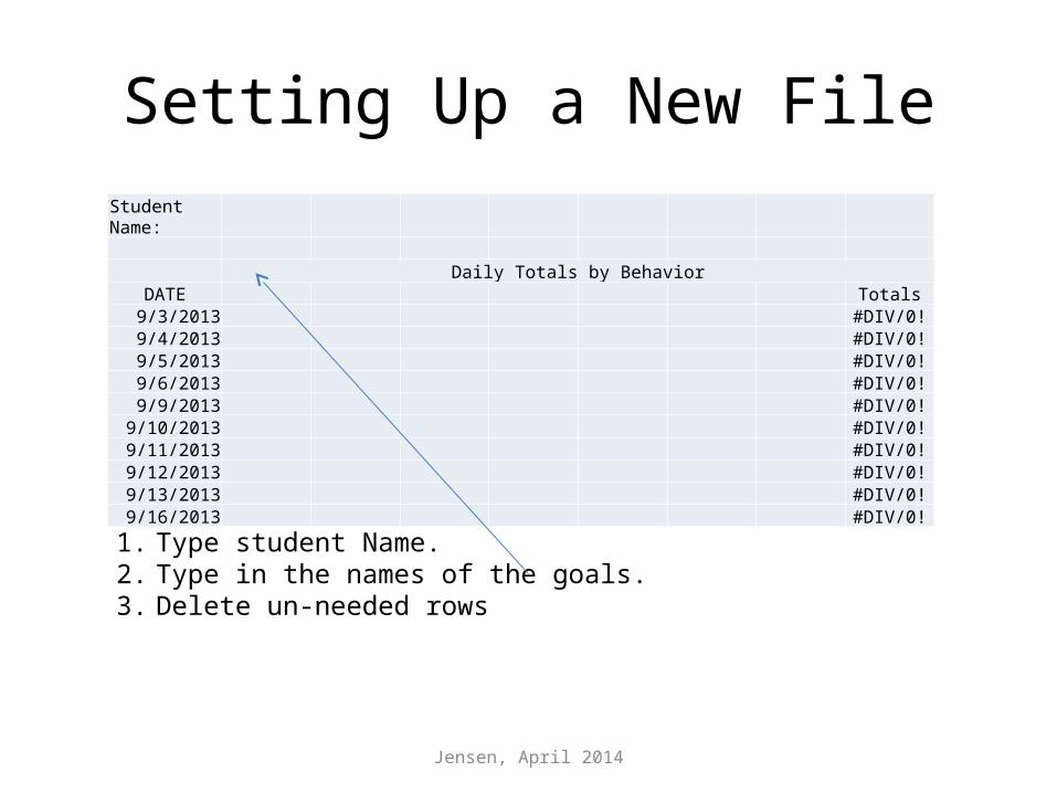
Setting Up a New FileStudent Name:

Daily Totals by BehaviorDATE Totals9/3/2013 #DIV/0!9/4/2013 #DIV/0!9/5/2013 #DIV/0!9/6/2013 #DIV/0!9/9/2013 #DIV/0!

9/10/2013 #DIV/0!9/11/2013 #DIV/0!9/12/2013 #DIV/0!9/13/2013 #DIV/0!9/16/2013 #DIV/0!

1. Type student Name.2. Type in the names of the goals.3. Delete un-needed rows

Jensen, April 2014

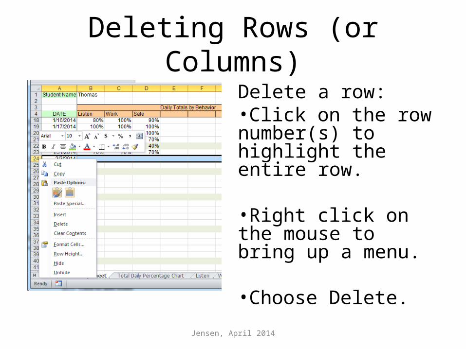
Deleting Rows (or Columns)

Delete a row:•Click on the row number(s) to highlight the entire row.

•Right click on the mouse to bring up a menu.

•Choose Delete.

Jensen, April 2014

Add a row:•Click on the row number to highlight the row.

•Right click on the mouse to bring up a menu.

•Choose Insert.

•A row will be added above the row you highlighted.

Adding a Row (or Column)

Jensen, April 2014

Formulas

Addition:=sum(A1:A5)

Average:=Average(A1:A5)

Percentage=(A1/A5)

Jensen, April 2014

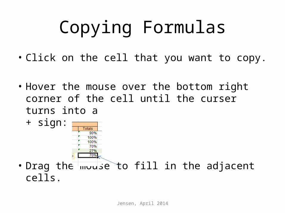
Copying Formulas

• Click on the cell that you want to copy.

• Hover the mouse over the bottom right corner of the cell until the curser turns into a + sign:

• Drag the mouse to fill in the adjacent cells.

Jensen, April 2014

Formatting Cells

Options:•Text•Number•Percentage

Jensen, April 2014

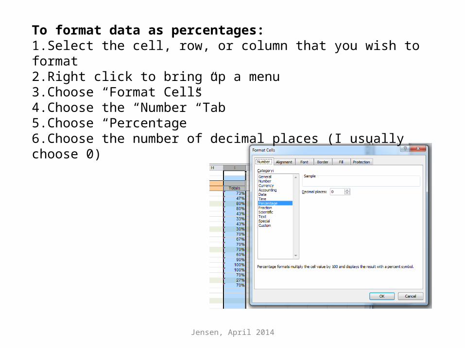
To format data as percentages:1.Select the cell, row, or column that you wish to format2.Right click to bring up a menu3.Choose “Format Cells”4.Choose the “Number” Tab5.Choose “Percentage”6.Choose the number of decimal places (I usually choose 0)

Jensen, April 2014

Updating Graphs

Jensen, April 2014

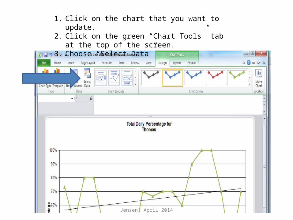
1. Click on the chart that you want to update.2. Click on the green “Chart Tools” tab at the top of the

screen.3. Choose “Select Data”

Jensen, April 2014

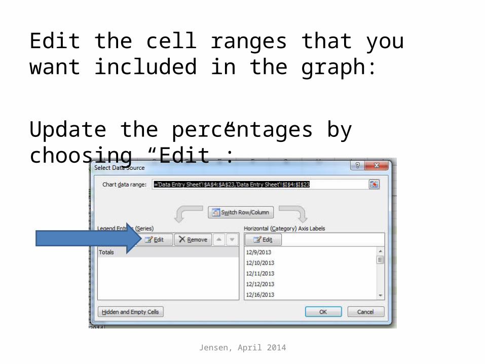
Edit the cell ranges that you want included in the graph:

Update the percentages by choosing “Edit”:

Jensen, April 2014

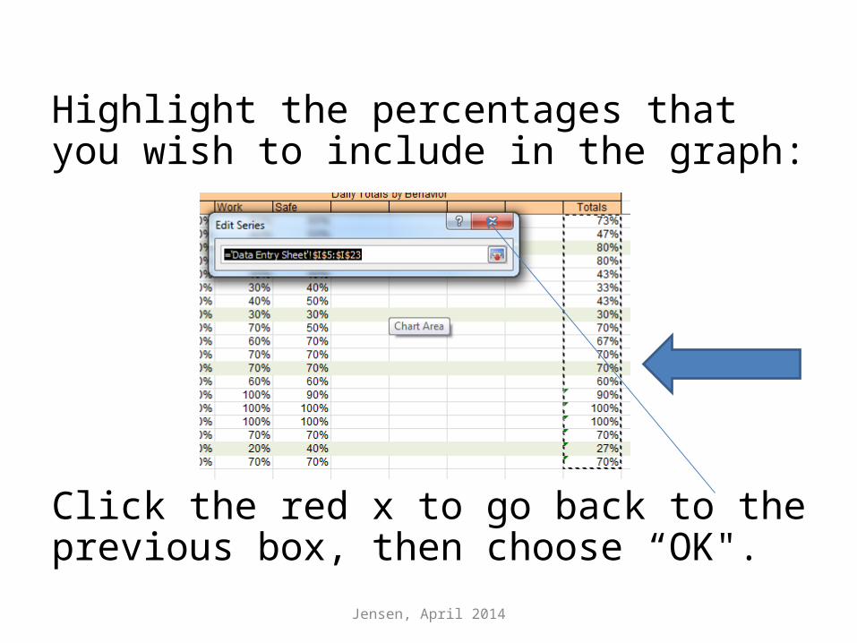
Highlight the percentages that you wish to include in the graph:

Click the red x to go back to the previous box, then choose “OK".

Jensen, April 2014

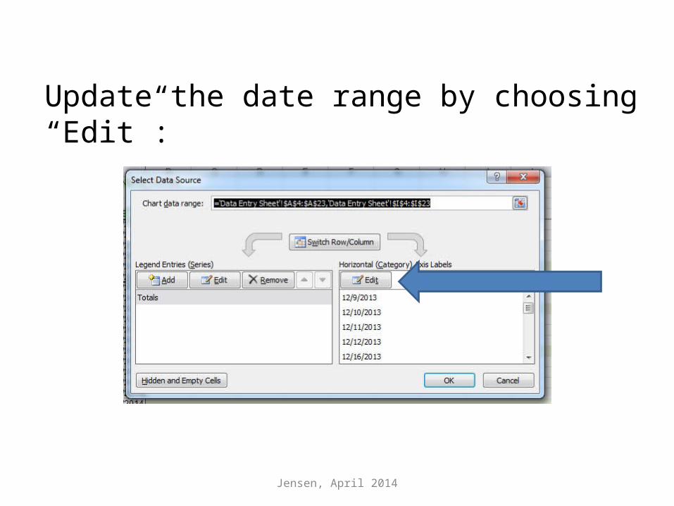
Update the date range by choosing “Edit”:

Jensen, April 2014

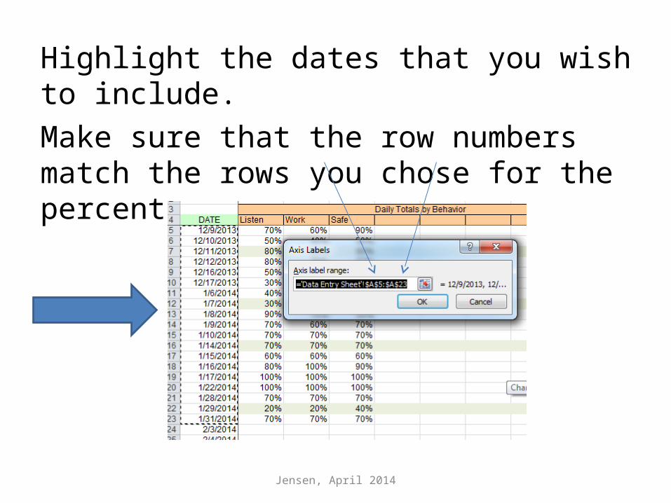
Highlight the dates that you wish to include. Make sure that the row numbers match the rows you chose for the percentages.

Jensen, April 2014

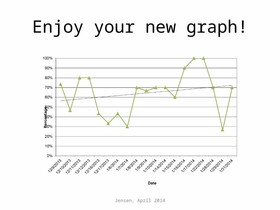
Enjoy your new graph!

Jensen, April 2014

Troubleshooting:

• Div/0 errors• Funny-looking trendlines• Adding variables will sometimes cause the

dates to disappear.

Jensen, April 2014

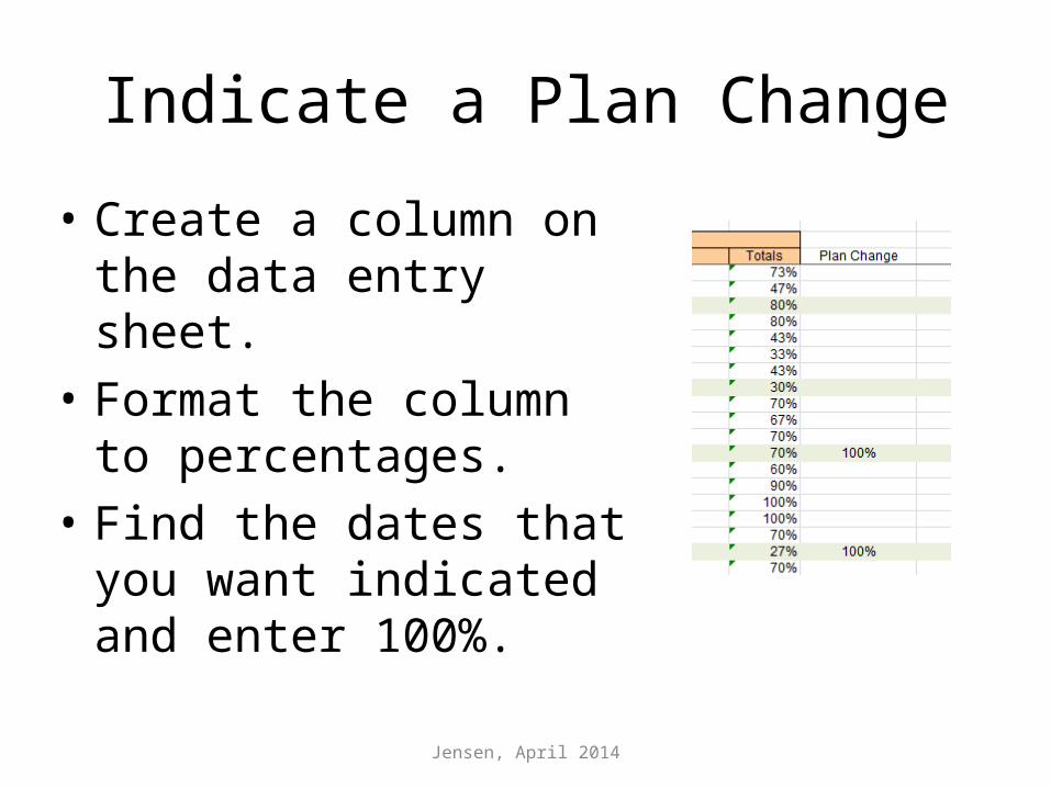
Indicate a Plan Change

• Create a column on the data entry sheet.

• Format the column to percentages.

• Find the dates that you want indicated and enter 100%.

Jensen, April 2014

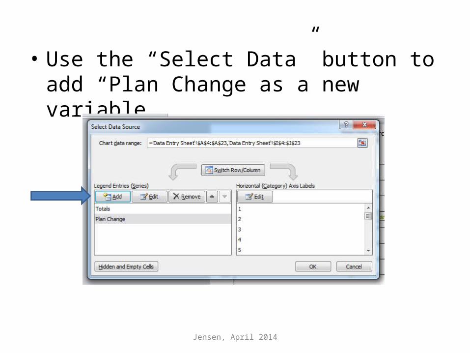
• Use the “Select Data” button to add “Plan Change as a new variable.

Jensen, April 2014

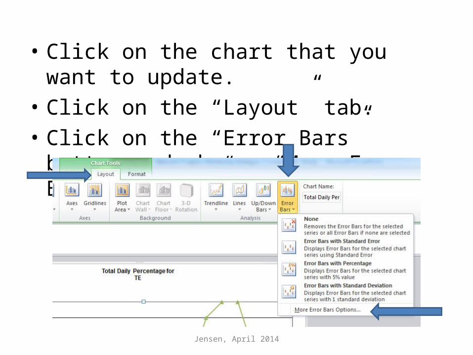
• Click on the chart that you want to update.• Click on the “Layout” tab.• Click on the “Error Bars” button and choose

“More Error Bars Options…”

Jensen, April 2014

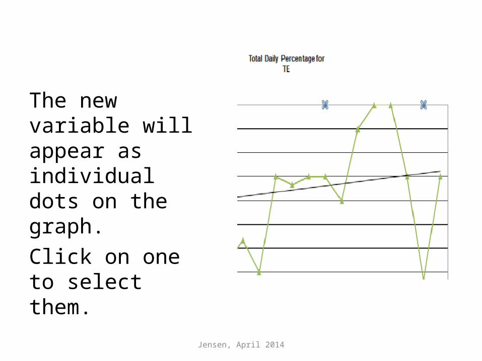
The new variable will appear as individual dots on the graph. Click on one to select them.

Jensen, April 2014

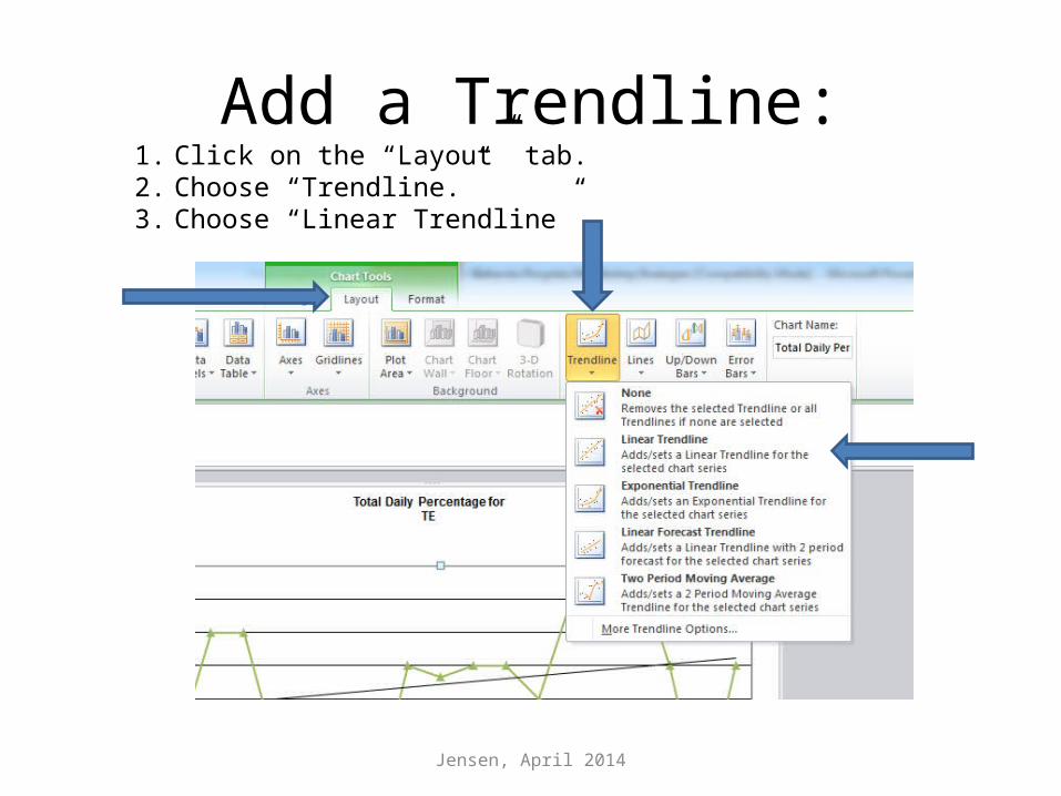
Add a Trendline:1. Click on the “Layout” tab.2. Choose “Trendline.”3. Choose “Linear Trendline”

Jensen, April 2014

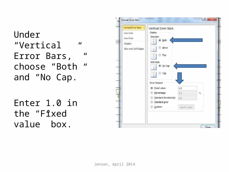
Under “Vertical Error Bars,” choose “Both” and “No Cap.”

Enter 1.0 in the “Fixed value” box.

Jensen, April 2014

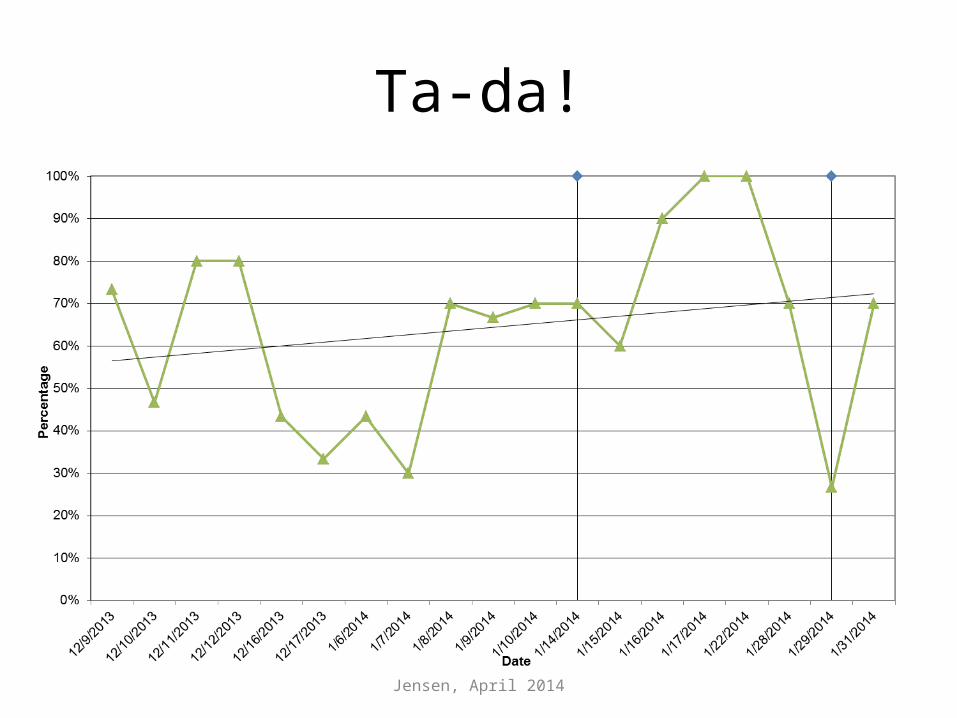
Ta-da!

Jensen, April 2014