Embed Size (px)
Citation preview

KAUNO TECHNOLOGIJOS UNIVERSITETAS
Vaidotas Marozas
Biomedicininių signalų skaitmeninis netiesinis
filtravimas
Daktaro disertacija
Technologijos mokslai, Elektros ir elektronikos inžinerija (01T)
Kaunas 2000

Darbas atliktas 1995-2000 metais Kauno technologijos universitete.
Doktorantūros teisė suteikta 1992 10 07 Lietuvos Respublikos
Vyriausybės nutarimu Nr.739.
Doktorantūros komitetas:
pirmininkas ir darbo vadovas:
prof. habil. dr. (technologijos mokslai, elektros ir elektronikos
inžinerija, 01T) Arūnas. Lukoševičius (Kauno technologijos universitetas);
nariai:
prof. habil. dr. (technologijos mokslai, elektros ir elektronikos
inžinerija, 01T) Danielius Eidukas (Kauno technologijos universitetas);
prof. habil.dr. (technologijos mokslai, elektros ir elektronikos
inžinerija, 01T) Stanislovas Sajauskas (Kauno technologijos
universitetas);
prof. habil. dr. (technologijos mokslai, elektros ir elektronikos
inžinerija, 01T) Rymantas Jonas Kažys (Kauno technologijos
universitetas);
doc.dr. (medicinos mokslai, medicina, 07B)
Alvydas Paunksnis (Kauno medicinos universitetas).

KAUNAS UNIVERSITY OF TECHNOLOGY
Vaidotas Marozas
Non-linear digital filtering of biomedical signals
Doctoral dissertation
Technology sciences, electrical and electronics engineering (01T)
Kaunas 2000

2
Abstract The aim of this dissertation is to investigate the benefits of using wavelet based time-
frequency analysis in filtering of non-stationary biomedical signals.
Filtering of non-stationary signals is an important issue in biomedical applications for increasing the accuracy of signal detection. One of possible applications of filtering methods is transient evoked otoacoustic emission (TEOAE), which is used to separate hearing impaired and normal hearing subjects in large screening tests of hearing. It is very important to have high sensitivity and specificity of these tests. Linear bandpass filtering was shown useful for increasing the specificity without loss of sensitivity in detection of TEOAE. However, linear filtering gave very limited improvement, since the spectrum of these signals is changing in time and overlaps with the spectrum of the noise.
In this dissertation, we have shown the use of wavelet transform for denoising of TEOAE signals using non-linear filtering and time- frequency filtering. Non- linear filtering, which is using the shrinkage of wavelet coefficients, was shown useful in applications, where spectrum of the signal and of the noise overlap. Very important issue is here to estimate the optimal shrinkage threshold. We developed the procedure to estimate this threshold. The threshold can be found by maximizing some criterion for optimality, e.g. cross correlation coefficient of the two subaverages of the TEOAE. The results of the non-linear filtering using proposed and thresholds found in the literature were compared. New threshold showed advantage over known thresholds. Another contribution of this dissertation is the method for time- frequency filtering of the signal using selection of the relevant signal expansion coefficients in discrete wavelet basis. The relevant coefficients can be determined by using a priori knowledge about the location of the signal components in time- frequency plane or by using statistical analysis, e.g. decomposing large amount of the signals and averaging them in time- frequency plane. Comparison of filtering results with proposed non-linear, time- frequency and known linear methods showed time-frequency filter being the best.
The feature extraction method using discrete orthonormal wavelet transform was investigated. The extracted features were cross correlation coefficients among in frequency and in time limited TEOAE signal components. It was shown how these features could be obtained very efficiently using fast discrete wavelet transform. A neural network was suggested for combining the extracted features. Comparison of the subjects' separation results in large database of TEOAE signals using proposed and known in literature filtering methods and proposed feature extraction methods was made. Receiver operator characteristics were used for comparisons. The highest increase of specificity at the level of 90% of sensitivity was achieved by using neural network for combining the extracted TEOAE features: from 68% to 84%.

3
Contents
Abstract ............................................................................... 2
Contents .............................................................................. 3
1 Introduction ..................................................................... 6
2 Biomedical signals. Signals of transient evoked otoacoustic emission ......................................................................... 13
2.1 Biomedical signals in general .......................................................... 13
2.2 TEOAE signal .................................................................................. 14
3 Classical and new solutions of biomedical signal enhancement and detection ............................................ 17
3.1 Averaging ........................................................................................ 17
3.2 Filtering .......................................................................................... 18
3.3 Detection ........................................................................................ 20
4 Wavelets and wavelet transform ...................................... 23
4.1 Wavelet theory ................................................................................ 23
4.2 Properties of wavelet transform ....................................................... 28
4.2.1 Locality in time- frequency ...................................................... 28
4.2.2 Energy concentration .............................................................. 29
4.2.3 Energy preservation ................................................................ 33
4.2.4 Fast implementation ............................................................... 33
5 Non-linear filtering ......................................................... 35
5.1 Wavelet transform of the signal with noise ....................................... 35
5.2 Wavelet coefficient shrinkage for non-linear filtering ........................ 36
5.2.1 Non-linear shrinkage functions ............................................... 36
5.2.2 Threshold estimation............................................................... 37

4
5.2.3 Alternative method for threshold estimation ............................ 39
5.3 Wavelet coefficient selection for time- frequency filtering .................. 40
5.4 Simulations. Comparison of the different denoising methods ........... 43
5.4.1 Data set for experiment ........................................................... 43
5.4.2 The denoising parameters and measures of performance ......... 44
5.4.3 Simulation results ................................................................... 45
5.4.4 Summary ................................................................................ 50
6 Time- frequency feature extraction for signal detection .. 52
6.1 Correspondence of cross correlation calculations in time domain and in wavelet domain .......................................................................... 52
6.2 Time windowing in wavelet domain .................................................. 53
6.3 Artificial neural network for signal detection .................................... 55
7 Applications and algorithms ........................................... 57
7.1 Wavelet based TEOAE denoising and detection ................................ 57
7.2 Experimental data ........................................................................... 58
7.3 Wavelet based TEOAE denoising...................................................... 59
7.3.1 Algorithms .............................................................................. 59
7.3.2 Other methods for signal-to-noise ration improvement in TEOAE records ................................................................................... 59
7.3.3 TEOAE denoising results with different methods ..................... 59
7.3.4 Discussion .............................................................................. 62
7.4 TEOAE feature extraction and detection .......................................... 64
7.4.1 Feature average based detector ............................................... 65
7.4.2 Neural network based detector ................................................ 66
7.4.3 Statistical decision theory for the comparison of the detectors . 67
7.4.4 Subject separation results when separation parameter is an average of the features extracted from TEOAE ........................ 68
7.4.5 Comparison of linear and non-linear TEOAE detectors in hearing screening ................................................................................ 70
7.4.6 Discussion .............................................................................. 73
8 Conclusions .................................................................... 77

5
Acknowledgements ............................................................. 79
Bibliography ....................................................................... 80
Appendix ............................................................................ 88
1 Simulation of the system “Kemp’s hearing faculty tester and TEOAE emitting auditory periphery” ........................ 89
1.1 Kemp’s hearing faculty tester .......................................................... 93
1.2 SIMULINK model of Kemp’s hearing faculty tester ........................... 95
1.3 SIMULINK model of TEOAE producing ear ....................................... 98
1.4 Results of the system simulation ................................................... 100

6
1 Introduction
Most of biomedical signals are non-stationary, very low in amplitude and
usually are embedded in noise of various origins: environmental noises,
noise of the recording hardware, subject generated noise and other. To
remove these noises from the signal it is impossible to use classical filtering
because in most of the cases spectra of the signal and of the noise overlap.
Another problem is the detection of biomedical signals. This task we
formulate as making the decision whether a recorded waveform consists of
"noise alone" or "signal masked by noise". The detection of biomedical signals
is more difficult than of radar as the shape of the signal is usually unknown.
In addition, the recorded waveforms exhibit high variability among the
subjects with similar parameters. Thus, the most salient features that are
characteristic to signal class of interest should be established. This problem
can be reformulated as feature extraction.
New emerging tool for signal analysis, a wavelet transform, was shown
useful in the processing of non-stationary signals. Thus, it was decided to
investigate the benefits of moving from time domain to wavelet domain in the
processing of biomedical signals: transient evoked otoacoustic emissions.
The aim. The aim of this dissertation is to investigate and to develop new
wavelet analysis based methods for denoising and detection of complex, non-
stationary biomedical signals and to adopt them to the signals of transient
evoked otoacoustic emission.
Novelty. The framework of signal denoising and detection in the discrete
wavelet transform domain is established. New threshold estimation method
was proposed in wavelet based denoising of signals of transient evoked
otoacoustic emission. Novel, wavelet coefficient selection based denoising
method, was developed. Time-frequency features and neural network to
combine these features were suggested in the problem of transient evoked
otoacoustic emission signal detection.
Practical implementation. All the developed methods and algorithms
were designed taking in to account speed and practical implementation.
They were implemented using scientific computing language Matlab5.3,
MathWorks, Inc., which is becoming a standard in computation science and
engineering.
Reliability of the results. All the developed new algorithms were tested
on the large database consisting of 5213 signals.

7
The statistical hypothesis test was used to check if the difference between
the methods was statistically significant. Although the resulting difference
between the two signal classification methods was small, the hypothesis test
showed that we could reject the null hypothesis, as the evaluated P value
was 0.0002.
With this dissertation author defends the following conclusions:
1. The methods based on time- frequency (time- scale) signal
decompositions are more suitable for filtering and detection of non-
stationary biomedical signals when comparing with methods based only
on time or frequency analysis.
2. The feature of wavelet transform to concentrate the energy of the
correlated signal into a few high energy coefficients while scattering the
energy of the noise into many low amplitude coefficients can be used for
the non-linear filtering. Non-linear filtering of the signal can be
accomplished by the non-linear processing of the wavelet coefficients.
3. The results of wavelet based non-linear filtering depend on the used
analyzing wavelet. We have formulated the criterion of the optimality of
the wavelet for the given signal. It is a measure of the energy
concentration expressed as Shannon entropy. In case of otoacoustic
emission the best results among orthogonal wavelets with finite time
support showed "Symmlet 8" wavelet.
4. The optimal threshold for non-linear wavelet shrinkage can be estimated
by solving the problem of the maximization of some optimality criterion.
In case of otoacoustic emission, the cross correlation coefficient between
subaverages can be used as the criterion of the optimality.
5. The feature of wavelet transform to localize in time and in frequency at
the same instant can be used to establish the statistical location of the
non-stationary signal components in time- frequency plane and for time-
frequency filtering.
6. The cross correlation coefficients calculated among time and frequency
limited components of the signal can be used as the features for the
TEOAE signal detection. These features can be very efficiently calculated
directly in wavelet domain.

8
7. Wavelet based TEOAE filtering enabled to increase the specificity of the
TEAOE signal detection by 16% without any decrease of the sensitivity.
8. The neural network was suggested for combining the extracted features in
the application of separation hearing impaired and normal hearing
subjects. However, the increase in accuracy of the subject separation is
small when comparing with feature combiner, which uses average of the
features. This suggests similar weights of the features.

9
Outline of the dissertation contents
Wavelet based denoising and detection of
biomedical signals
Wavelet transform and its properties
Review of the problems of signal
denoising and detection
Wavelet based
denoising
Wavelet based feature
extraction
Database of real
TEAOE signal
records
Results
And
Discussion
Results
And
Discussion
Conclusions
Biomedical signals in general.
TEOAE signals

10
List of publications by the author of the dissertation
Journal papers:
1. Marozas V., Lukoševičius A., Engdahl B., Svensson O. and Sörnmo L.
"Otoacoustic emissions and pass/fail separation using artificial neural
network". Ultragarsas, 1(34), pp. 7-12, 2000.
2. Marozas V., Janušauskas A., Engdahl B., Svensson O. and Sörnmo L.
"Detection of otoacoustic emission in the wavelet domain". Medical &
Biological Engineering & Computing, Suppl. vol. 37, pp.334-335, 1999.
3. Marozas V. "Vienmačio nestacionaraus signalo skleidimo laiko ir dažnio
plokštumoje metodai ir jų pritaikymas otoakustinés emisijos signalo
analizei". Elektronika ir elektrotechnika, 3(12), pp.18-20, 1997.
4. Janušauskas A., Marozas V., Engdahl B., Svensson O. and Sörnmo L.
"Otoacoustic emissions and improved pass/fail separation using wavelet
based de-noising". Accepted for publication in Medical and Biological
Engineering and Computing, 2000.
5. Janušauskas A., Marozas V., Engdahl B., Svensson O. and Sörnmo L.
"Wavelet based denoising of otoacoustic emissions". Elektronika ir
elektrotechnika, 5(18): 38-41, 1998.
Conferences and workshops:
1. Marozas V., Lukoševičius A., Svensson O., Engdahl B. and Sörnmo L.
"Wavelets for feature extraction and neural network for detection of
otoacoustic emission". Biomedical engineering'99, KTU, Kaunas, October
1999.
2. Janušauskas A., Marozas V., Engdahl B., Svensson O. and Sörnmo L.
"Otoacoustic emissions and improved pass/fail separation using wavelet
based denoising". Annual International Conference of the IEEE
Engineering in Medicine and Biology Society, Hong Kong, pp. 3129- 3131,
1998.

11
3. Marozas V., Janušauskas A., Svensson O. and Sörnmo L. "New method
for detection of otoacoustic emission and comparison with other methods".
Biomedical engineering'98, pp. 90-93, KTU, Kaunas, October 1998.
4. Marozas V., Janušauskas A. ir Lukoševičius A. "Otoakustinés emisijos
(OAE) fenomenas. Metodas OAE signalų charakterizacijai". Biomedical
engineering'97, pp. 86-89, Kaunas, KTU, October 1997.
5. Marozas V., Janušauskas A., Lukoševičius A., Engdahland B.,
Svensson O. and Sörnmo L. "Wavelets and Neural Networks in Detection
of Otoacoustic Emission" Workshop "Advances in Signal and Image
Processing for Solving Real Problems of the Real World" Nida, Lithuania,
August, 1999.
Technical reports:
6. Marozas V. "Modeling of the Hearing System". In the report BK8-11
"Investigation of acoustic medical diagnostic systems and signals" by
A.Lukoševičius, D. Jegelevičius, R. Jurkonis, V. Marozas, A Janušauskas,
Kaunas, KTU, 1998.

12
Abbreviations ANN Artificial neural network
DFT Discrete Fourier transform
DWT Discrete wavelet transform
FN False negative
FP False positive
GCV Generalized cross validation
HI Hearing impaired subject
HTL Hearing threshold levels
MAD Median Absolute Deviation
MHL Mean hearing level
MLP Multilayer perceptron
MRA Multiresolution analysis
MSE Mean square error
NH Normal hearing subject
OAE Otoacoustic emission
PSD Power spectral density
ROC Receiver operator characteristic
SNR Signal-to-noise ratio
SPL Sound pressure level
STFT Short time Fourier transform
SURE Stein’s Unbiased Risk Estimate
TEOAE Transient evoked otoacoustic emission
TN True negative
TP True positive
Notation j - Level of the wavelet decomposition
2j - Dyadic scale
1/2j - Resolution
J - Maximal level of decomposition
L -Length of the filter involved in
wavelet decomposition
O -"Order of …" (in counting the
number of operations)

13
2 Biomedical signals. Signals of transient evoked otoacoustic emission
2.1 Biomedical signals in general
A signal is a phenomenon, which carries information. Biomedical signals
are signals that emanate from living systems. The analysis of these signals
gives the information about the living system, which created the signal.
Biomedical signals are used for diagnostic, monitoring and other goals.
The process of information extraction can be simple as inspection by
experienced eye of physician. However, often in biomedical applications the
acquisition of the signal is not enough. It is required to process the signal to
get the information, which is hidden in it. This may be because of the noise
in the signal. Therefore, information cannot be seen with the "naked eye".
The signal must be "cleaned". Different terms are used to describe this
process: signal recovering, signal enhancing or signal denoising.
The biomedical signals are classified according to their origin: bioelectric,
bioacoustic, bioimpedance, biomechanical, biooptical, biomagnetic,
biochemical signals. Further, they can be divided into two main groups:
deterministic and stochastic. Deterministic signals can be divided in periodic
and non-periodic, while stochastic signals- into stationary and non-
stationary. Such a vast variety of biomedical signals do not allow creating
the universal methods, suitable for the processing of all the biomedical
signals. Thus, it is a very important task today to identify the methods that
are suitable for the particular signal classes and in opposite- to define the
classes of the signals that can be treated with the particular method.
Another important task is to achieve a full success in the particular
application and to make a step further by identifying signal specific features
and incorporation of all the a priori known information about the signal and
system under investigation.
In this investigation we will consider biomedical signal enhancement
methods with the application to one of the bioacoustic signals- transient
evoked otoacoustic emission (TEOAE), which can be used to extract
information about the state of the hearing organ- cochlea.

14
2.2 TEOAE signal
TEOAE is low-level sound produced by the cochlea as the response to the
short acoustical stimulus. TEOAE is present usually in the normal hearing
ear but absent, or attenuated, in the dysfunctional cochlea [47].
Gold [32] was the first who hypothesized otoacoustic emission in 1948
and Kemp [47] was the first who recorded it in 1978. There is still no
complete theory explaining TEOAE generation, yet. It is believed that the
TEOAE is partial product of amplification process, which is present in the
cochlea [35].
The main properties that characterize the TEOAE are:
1. Non-linearity. Due to the non-linear nature of cochlear preprocessing of
sound, the presentation of different frequencies leads to the generation of
several additional combination frequencies. In addition, the physical
properties of the basilar membrane mechanics in the cochlea change with
stimulus level. This "compressive" non-linearity leads to compressive
amplitude growth functions in the TEOAE acquisition. This property is
used to separate the linear acoustical stimulus from non-linear response
in time with the technique called "non-linear differential averaging" [6]
2. Dispersion. Otoacoustic emissions (OAE) are delayed with respect to the
onset of acoustical stimulation. OAE exhibit strong dispersion. The
latency of otoacoustic emissions increases from approximately 3 ms at
frequencies of about 6 kHz to more than 10 ms at frequencies near 1 kHz.
Changing spectral characteristics of TEOAE signal causes it to be non-
stationary in time, which causes problems for signal filtering from the
noise. Investigation of latencies of different frequency components in
TEAOE signal attracted much of attention [40], [91], [92], [94], [58].
3. Reproducibility. Otoacoustic emissions are highly reproducible. The
temporal and spectral properties of OAE are unique for each subject and
are stable for long time ("fingerprint of the inner ear"). Because of this
feature TEOAE signal can be treated as deterministic for the same subject
and signal averaging technique can be used in order to increase signal to
noise ratio.
PC based systems are used for TEOAE recording. The click stimulus is
produced by application of an 80 µs electrical pulse to the speaker in the ear
canal probe. Stimuli are presented at a rate of 50 Hz. The stimulus voltage
results in click levels of approximately 80 dB SPL in adult ears. The stimuli
have flat spectra up to 4-5 kHz in the ear canal. The ear canal sound

15
pressure is sampled at 25.6 kHz for 20 ms after each stimulus with a 12-bit
analog-to-digital converter and alternate samples are stored in separate 512-
point waveform buffers, resulting in two waveforms.
Stimulus generator
Stimulus
ADC
GATE
Microphone
Speaker
Ear
Bufer A
Bufer B
Signal processing
algorithms
Figure 2.1 System for TEOAE signal acquisition (ADC- analog to digital converter)
The typical example of two subaveraged TEOAE waveforms is shown in
Figure 2.2. Earlier described different features can be identified: both
waveforms exhibit shorter periodicities or higher frequencies at shorter post
stimulus times and both subaveraged waveforms show very high similarity
or reproducibility in this case.
0 5 10 15 20
-4
-3
-2
-1
0
1
2
3
4
x 10-4
Pre
ssure
, P
a
Time, ms
ρ=99%
Figure 2.2 Example of TEOAE subaverages as recorded from a normal hearing subject having mean hearing threshold 9dB
Although TEOAE is mainly object of the research yet, applications in
clinical practice appear. TEOAE appeared to be useful in screening tests in
16
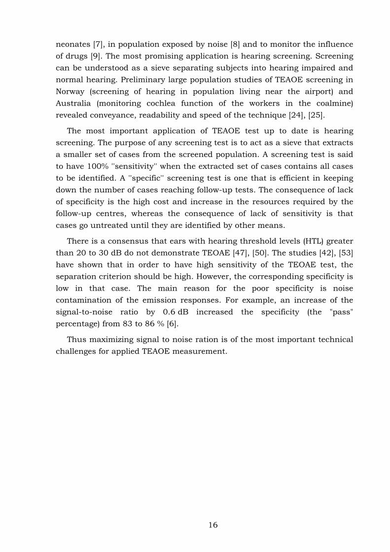
neonates [7], in population exposed by noise [8] and to monitor the influence
of drugs [9]. The most promising application is hearing screening. Screening
can be understood as a sieve separating subjects into hearing impaired and
normal hearing. Preliminary large population studies of TEAOE screening in
Norway (screening of hearing in population living near the airport) and
Australia (monitoring cochlea function of the workers in the coalmine)
revealed conveyance, readability and speed of the technique [24], [25].
The most important application of TEAOE test up to date is hearing
screening. The purpose of any screening test is to act as a sieve that extracts
a smaller set of cases from the screened population. A screening test is said
to have 100% ''sensitivity'' when the extracted set of cases contains all cases
to be identified. A ''specific'' screening test is one that is efficient in keeping
down the number of cases reaching follow-up tests. The consequence of lack
of specificity is the high cost and increase in the resources required by the
follow-up centres, whereas the consequence of lack of sensitivity is that
cases go untreated until they are identified by other means.
There is a consensus that ears with hearing threshold levels (HTL) greater
than 20 to 30 dB do not demonstrate TEOAE [47], [50]. The studies [42], [53]
have shown that in order to have high sensitivity of the TEOAE test, the
separation criterion should be high. However, the corresponding specificity is
low in that case. The main reason for the poor specificity is noise
contamination of the emission responses. For example, an increase of the
signal-to-noise ratio by 0.6 dB increased the specificity (the "pass"
percentage) from 83 to 86 % [6].
Thus maximizing signal to noise ration is of the most important technical
challenges for applied TEAOE measurement.

17
3 Classical and new solutions of biomedical signal enhancement and detection
We review classical methods of biomedical signal denoising and detection
in this section. We formulate the problems associated with these approaches
and point out the directions to solve them.
3.1 Averaging
The basic method used for enhancing biomedical signals including
TEAOE is to make an average of the recorded signal obtained from several
consecutive stimuli [88]. The signal must satisfy the following conditions in
order to achieve good results:
1. The signal epochs should contain a deterministic signal component,
which does not vary for all the epochs
2. The contaminating noise is a broadband stationary process with zero
mean and variance σ2.
3. Signal f[n] and noise v[n] are uncorrelated so that the recorded signal
s(t) at the i-th realization can be expressed:
]n[v]n[f]n[s ii += ( 3.1 )
After N time averaging it can be written:
∑∑∑===
+=N
i
i
N
i
i
N
i
i ]n[vN
]n[fN
]n[sN
111
111 ( 3.2 )
If all the previous conditions are satisfied the averaging result is:
∑=
+=N
i
ii ]n[vN
]n[f]n[s1
1) ( 3.3 )
The averaged noise signals variance σ2 decreases N times and
improvement in SNR (rms value) is √N.
An example of the TEOAE signal subaverages with different numbers of
realizations included in the average is shown in Figure 3.1.
One of main drawbacks of such estimator is long averaging time to
achieve signal estimate with suitable SNR for further analysis. In addition,
the conditions for background noise normality can be broken during long

18
averaging time. Thus, in general averaging time is limited and other
techniques for further signal enhancement are sought.
Figure 3.1 Enhancement of TEOAE signal by means of averaging technique. The noise is progressively reduced by increasing number of sweeps
N in each subaverage. ρ is the cross correlation coefficient between subaverages.
3.2 Filtering
Averaged signal estimate can be further enhanced with linear filter by
exploiting the fact that the spectra of noise and response do not completely
coincide. In case of standard TEOAE acquisition procedure two filters are
used: low-pass with the cut-off 6.4 kHz to exclude instrumentation noise
and high-pass, with the cut-off 0.6 kHz to exclude some of the stimulus
artefact and the largest components of ambient and subject generated
noise [6].
The performance of a filtering procedure in reducing noise of TEAOE can
be improved by optimising the frequency response of the filter. Optimisation
of the cut-off frequency of the high pass filter has been performed in
study [93]. The criterion for the optimum frequency was maximal
reproducibility of the responses with the constrain to the loss of the cross-

19
spectral energy. The same strategy was used in study [78] with the difference
that bandpass filter was used instead of high pass and both cut-off
frequencies low and high were optimised. The best results of the optimal
filter in terms of increasing the post-filtering reproducibility was obtained
when the procedure was applied to recordings whose reproducibility before
filtering ranged between 60 and 80 %, i.e. for responses classified as partial
pass.
However, when the PSD of signal and noise overlap the highest increase
in SNR with lowest distortion to the signal can be obtained by Wiener
filtering approach. The Wiener filter is given by the transfer function:
( ) ( )( ) ( )ωω
ωω
nnss
ss
SS
SH
+= ( 3.4 )
where Sss(ω) is power spectrum of the response and Snn(ω) is power
spectrum of the noise.
Figure 3.2 Filtering with Wiener filter: a) real TEOAE signal (SNR=∞), b) power spectrum of the clean signal, c) signal contaminated with white
Gaussian noise (SNR=0.6dB), d) power spectrum of contaminated signal, e) filtered signal (SNR=8.8) and f) transfer function of the Wiener filter
Since Sss(ω) and Snn(ω) are not known in advance they should be
estimated from the records [89]. Figure 3.2 shows the experiment where real
TEOAE signal (plot a) was contaminated with white Gaussian noise (plot c)
and the signal after filtering with Wiener filter shown in plot f. Plot b shows

20
power spectrum of the clean signal, plot d shows power spectrum of
contaminated signal. The gain in SNR after filtering is 7 dB. It is idealized
situation as in real conditions the quantities Sss(ω) and Snn(ω) are not known.
They have to be estimated from the recorded signal, thus errors in the
estimates will lead to the lower performance.
Another problem that faces Wiener filter, is non-stationary signals. The
Fourier transform is used to estimate the transfer function of the filter.
However, the Fourier transform is not localized in time space and removing
noise at a specific frequency with Wiener filter also involves removing any
signal components, which also share the same frequency. Thus, any change
made to a Fourier coefficient is a global, effecting both noise and signal.
To overcome the limitations of the Fourier analysis to represent non-
stationary signals, Short Time Fourier Transform (STFT) was proposed. It
contains the time parameter and the frequency parameter as well. The
localization in time is achieved by weighting or windowing previous infinite
Fourier basis functions. If the Gaussian function exp(-t2) is used as the
window function then it is known as the Gabor transform. The time
resolution of the STFT is given by the time width of the window function. The
spectrum is only captured with finite resolution, too. Here, the spectral
resolution is given by the bandwidth of the window function. The product of
the bandwidth and the time width of the window function is a constant,
which depends only on the shape of the window function. In the case of the
STFT, the division of the time-bandwidth product into time duration and
bandwidth is the same for all values of frequency and time. Thus, STFT has
a constant resolution. However, most of the biomedical signals are multi-
component in nature. They consist of high frequency components of shorter
duration and low frequency components of longer duration. STFT is not
adequate to such kind of signals. There was a need for the transform, which
divides the time-bandwidths product differently at different frequencies and
different times. This can be attained by the relatively new signal processing
tool- wavelet transform [16].
3.3 Detection
The signal detection problem is to decide whether the waveform consists
of "noise alone" or signal "masked by noise". Our goal is to use the received
data as efficiently as possible in making the decision while being correct
most of the time.

21
More formally detection problem in discrete function domain could be
formulated as "having received the signal s[n], form the function of the
received data d{s[n]} and when make the decision based on its value".
In clinical diagnostic applications, biomedical signals carry information,
which is often interpreted as "true negative" (TN) or "true positive" (TP). For
example, in TEOAE case, detected signal is interpreted as "negative" result
indicating normally functioning cochlea, while response, which shows no
TEOAE like activity is interpreted as "positive" result showing problems in
the cochlea.
Figure 3.3 Four members of the family of ROC curves. ROC curves are indexed over increasing range of SNR. The curve Nb. 1 indicates detection
performance at the lowest SNR, Nb.4- at the highest.
In practice we face with two problems when making the detection: how to
form the function d{s[n]} and where to set the decision threshold T on
function d{s[n]} so as to ensure that the number of decision errors is small.
There are two types of errors possible: the error of missing the signal (decide
"noise" when in reality is "signal+noise") and the error of false alarm (decide
"signal+noise" when only "noise" is present). In biomedical diagnostic
applications these errors are named "false positive" (FP) and "false negative"
(FN). In case of TEOAE based hearing test FP result would point to the
normally hearing subject as hearing impaired while because of FN result we
would miss the hearing impaired subject. The probability to detect correctly
normal hearing subject is named "Specificity" of the test. The probability to
detect correctly hearing impaired subjects is named "Sensitivity" of the test.

22
These probabilities can be varied by choosing different decision threshold T
in the output of the detector d{s[n]}. However, when one of the probabilities
is increased, the other is decreased. A function of sensitivity as a function of
the variable 1-specificity, when the decision threshold is varied over all range
of the detector d{s[n]} values, is called receiver operating characteristic
(ROC). Good detector should have ROC curves which have desirable
properties such as concavity (negative curvature), monotone increase in
sensitivity as specificity decreases, high slope of sensitivity at the point
(Sensitivity, 1-Specificity)=(0,0) [38]. Simply stated, the goal of signal
processing algorithms is to find ways to test between outcomes Negative and
Positive, which push the ROC curve towards the upper left corner of Figure
3.3, where both sensitivity and specificity are high. In practice, one operating
point or the threshold T is chosen to meet particular requirements of the
application. For example, in TEOAE based hearing test more important
parameter is sensitivity than specificity. Thus, it is usually chosen to be
high: 90 or 95 %.
Another issue in the signal detection problem is the determination of the
function d{s[n]}. This problem is known as pattern recognition problem [11].
It can be divided into the steps of feature extraction and combination of the
features to form the function d{s[n]}. The stage of feature extraction involves
the transformation of the received data s(n) in such a way as to reveal key
features of a signal that are difficult or impossible to discern in the original
domain. For example, Fourier transform reveals the composition of the
signal in terms of building blocks, or basis functions of transformed domain:
sines and cosines. Fourier transform depends on the one parameter-
frequency. Time dependence is lost in the transform. It cannot be seen when
exactly the spectral components of the signal appear and this is
unsatisfactory for non-stationary signals. Thus, wavelet transform was
planed to be used for extraction of the features.
The final issue in the construction of detection function d{s[n]} is how to
combine the extracted features. The features can be combined linearly and
non-linearly. The weights for linear combination of the features can be
chosen by doing regression analysis. However, the most exact detector can
be achieved by using a artificial neural network as the non-linear feature
combiner [37].

23
4 Wavelets and wavelet transform
In this section, we summarize some relevant aspects of wavelet theory,
which was introduced by Yves Meyer and Jean Morlet in 1984. Later in
section 4.2, we present some experiments and explorations of the relevant
properties of wavelet transform.
4.1 Wavelet theory
Every function can be expanded in such a way:
)()()( twttf j
j
jψµ ∑+= ( 2.1 )
where µ(t)- the mean of the function f(t), ψj(t)- system of elementary
functions and wj are expansion coefficients that are defined as:
∫∞
∞−
= dtttfw jj )()( *ψ ( 4.2 )
The possible examples of systems ψj(t) could be: signal dependant
Karhunen- Loeve basis of eigen functions [99], complex sines and cosines in
Fourier basis )exp()( tjt ωψ = . However, these functions are infinite in time
and are not suitable for characterization of non-stationary signals, spectral
characteristic of which are changing in time course. Another possibility is to
choose the system, which consist of elementary functions that are well
localized in time and frequency i.e. have rapid decay in time and frequency.
Elementary functions would behave as time- frequency atoms giving
possibility to represent the signal into joint time- frequency plane. Such
localized systems of elementary functions are short time Fourier transform
(STFT) and wavelet transform. The basis functions of STFT are windowed
sines and cosines:
)exp()()( tjtwt ωτψ −= ( 4.3 )
Where w(t) is window function, τ- shift in time parameter, ω- radial
frequency.
Basis functions of wavelet transform are defined as:

24
−=
abt
a)t(j ψψ 1 ( 4.4 )
Where
−
abtψ is mother wavelet, b- time shift parameter, a- scaling
parameter of the time variable t.
There are many such mother wavelets and many systems of wavelet
functions and wavelet transforms, which have different characteristics. Some
example analytic expressions and shapes of wavelets are shown below:
Morlet wavelet:
( ) eet tjt ωψ 0
2
2−= ( 4.1 )
Wavelet transform with this wavelet is expressed as:
( ) ( ) ( )dttf
a,aCWT ee a
tja
t
=
−−−
+∞
∞−∫
ττ ωτ 0
2
211 ( 4.2 )
"Mexican hat" wavelet:
( ) ( )ettt2
22
1 −−=ψ ( 4.3 )
and wavelet transform:
( ) ( ) ( ) ( )dt
attf
a,aCWT e a
t
−−=
−−∞+
∞−∫
τττ2
212
11 ( 4.4 )
With continuous parameters a and b, wavelet transform is called
continuous wavelet transform (CWT) and is highly redundant having minor
practical importance.
-5 0 5-1
-0.5
0
0.5
1Morlet wavelet
-5 0 5-0.5
0
0.5
1Mexican hat wavelet
Figure 4.1 "Morlet" and "Mexican hat" wavelets

25
This redundancy is removed in another type of wavelet transform- the
discrete wavelet transform (DWT). Signal transformed into discrete wavelet
domain has as many coefficients as it has in original time domain. Another
advantage of DWT to CWT is existence of the fast decomposition and
reconstruction algorithm based on filter banks and changing of sample rate.
The DWT stems from multiresolutional analysis and filterbank theory
[57]. The multiresolutional analysis is a decreasing sequence of closed
subspace {Vj}, which approximate square integrable functions space in L2(R).
A discretized function f[n] is projected at each step j, onto the subset Vj. This
projection is defined as the scalar product noted aj, of f(n) with a scaling
function noted φ[n]:
]kn[]n[faj
njjk −= −∑ 2
2
1 φ ( 4.5 )
Here k is the translation parameter and j is the dilation parameter.
Scaling function φ[n] has the following property:
( ) ( )knkhn
k
−=
∑ φφ22
1 ( 4.6 )
The sequence h(k) is the impulse response of a low pass filter.
Each step smoothens the signal. The lost information can be restored
using the complementary subspace Wj+1 of Vj+1 in Vj. This subspace is
generated by a wavelet ψ(n) with integer translations and dyadic dilation; the
projection of f(n) on Wj is defined as:
]kn[]n[fwj
njjk −= −∑ 2
2
1 ψ ( 4.7 )
As the scaling function, the wavelet function has the following property:
( ) ( )kn kgn
k
−=
∑ φψ22
1 ( 4.8 )
The sequence g[k] is the impulse response of a high-pass filter.
Then the analysis is defined as:

26
k,j
n
k,j
k,j
n
k,j
a]kn[gw
a]kn[ha
1
1
221
221
−
−
∑
∑
−=
−=
( 4.9 )
For orthogonal wavelets, the restoration is performed with:
k,j
n
k,j
n
k,j
w]nk[g
a]nk[ha
1
1
22
22
+
+
∑
∑
−
+−=
( 4.10 )
Thus, the function f[n] can be represented as the finite summation:
]n[a]n[w]n[f k,J
k
kk,j
J
j k
k,j φψ ∑∑∑ +==1
( 4.11 )
The wavelet coefficients wj,k and scaling coefficients ak comprise the
wavelet transform. For a wavelet centred at time zero and frequency f, wjk
measures the content of the signal around the time 2jk and frequency 2-jf (or
level j). Wavelet transform of sampled signal can be computed extremely
efficiently using two-channel filter banks structure [56] as it is shown in
Figure 4.2.
h[n] 2
g[n] 2
h[n] 2
g[n] 2
h[n] 2
g[n] 2
f[n]
w2,k
w3,k
a3,k
w1,k
Figure 4.2 The DWT using multirate filterbank algorithm (g[n] is the
highpass filter, h[n] is the lowpass filter, ↓2 means down sampling operation). Wavelet coefficients W1,k represent the first level of decomposition (j=1), W2,k
represent the second level of decomposition (j=2),
When a signal has n samples, they are ordered in wavelet domain as
follows:

27
n / 2n / 4
w1,kw2,kw3,k
aJ,k
n / 8 n
Figure 4.3 The order of the wavelet coefficients from different levels of wavelet decomposition in the vector of coefficients after wavelet
transformation. Here n is the number of samples in the signal in the original time domain
For DWT and IDWT structures shown in Figure 4.2 and Figure 4.4 to be
valid, the coefficients of the filters g[n] and h[n] have to be chosen carefully.
They have to satisfy three groups of conditions [16]:
1. Conservation of area condition,
2. Accuracy condition,
3. Orthogonality condition.
Thus, it is not easy to find the filters g[n] and h[n] satisfying all previous
conditions and limited amount of wavelets for DWT were found. The most
popular are:
• Daubechies filters indexed by their length, Par, which may be one of
4,6,8,10,12,14,16,18, 20;
• Coiflet filters are indexed as 1,2,3,4 or 5;
• Symmlets are wavelets within a minimum size support and as
symmetrical as possible, as opposed to the Daubechies filters, which
are highly asymmetrical. They are indexed from 4 to 10.
These wavelet families differ in the smoothness and compactness of the
basis functions.
h'[n] 2
g'[n] 2
h'[n] 2
g'[n] 2
h'[n] 2
g'[n] 2
f[n]
w2,k
w3,k
a3,k
w1,k

28
Figure 4.4 The IDWT using filterbak (g'[n] and h'[n] are reversed versions
of filters g[n] and h[n], ↑2 upsampling operations)
Examples of some typical orthogonal and finite in time wavelets are
shown in Figure 4.5.
Figure 4.5 Examples of compactly supported orthogonal wavelets
4.2 Properties of wavelet transform
4.2.1 Locality in time- frequency
Wavelet basis functions are localized in time and are scaled versions of
one mother function. A wavelet coefficient shows how much of the
corresponding wavelet basis function ‘is present’ in the total signal: a high
coefficient means that at the given location and scale there is an important
contribution of a singularity. This information is local in time and in frequency
(frequency is approximately the inverse of scale).
Figure 4.6 shows six wavelets from the same family Symmlet 8 and
corresponding frequency bands. Numbers in the brackets correspond to j,
which shows the level of decomposition or the location of wavelet in
frequency axis, and k is interpreted as the location of wavelet in time axis.
Figure 4.3 shows that there are n/2 wavelets in the first level i.e. j=1, n/4
wavelets in the level j=2 level there are n/4 wavelets and so on, where n is
number of samples in original time domain. Thus, time resolution decreases
in time level j or equivalently frequency is increasing. However, frequency
resolution is increasing when level increases (the second plot in Figure 4.6 ).

29
In conclusion, wavelet coefficient carries local information. Manipulating
of the wavelet coefficients causes a local effect, both in time and in
frequency.
Figure 4.6 Symmlet 8 wavelet examples ψj,k corresponding to different locations in time k and representing different frequency bands j. Here f is
sampling frequency
4.2.2 Energy concentration
Wavelet transform of a smooth signal is concentrated in relatively small
number of wavelet coefficients. On the other hand, the transform of a white
noise signal spreads out over all coefficients.
For example, signal representations in time domain, frequency domain
and wavelet domain were compared in terms of energy concentration in a few
large coefficients. Signals, shown in Figure 3.1 and white Gaussian noise
were used for the experiments.
Figure 4.7 shows three representations of white Gaussian noise: in time
domain, frequency domain and wavelet domain. Coefficients were taken in
absolute value, normalized to the range 0-1 and sorted in descending order.

30
Figure 4.7 Coefficients from different signal representations sorted in ascending order. TD - time domain coefficients, DFT- discrete Fourier transform
coefficients, DWT- discrete wavelet transform coefficients. For the DWT Symmlet 8 as mother wavelet was used.
Is obvious that curves of sorted DFT and DWT coefficients coincide,
showing that no one is better in compaction of white Gaussian noise.
Surprisingly, time domain representation of white Gaussian noise is more
compact as it has less large coefficients than other representations.
Figure 4.8 shows experiment with "correlated" signals that are depicted in
Figure 3.1. However, in this case, time domain representation of the signal is
the most "expensive": representation uses many large coefficients. In
frequency domain, signals are more concentrated than in time domain,
however wavelet representation shows the highest concentration of signal
energy in a few large coefficients. Especially it is noticeable at low SNR
(compare 2dB and 15dB plots in Figure 4.8).
The energy concentration ability of wavelet transform depends on the
number of vanishing moments m of mother wavelet ψ [95] :

31
( ) 1-m0,....,k ,xR
k
x ==∫ 0ψ ( 4.12 )
Wavelet transform, which uses mother wavelet with many vanishing
moments, is able to concentrate smooth signal very efficiently. However, the
number of vanishing moments defines the number of coefficients N used in
wavelet filter: N=2m. Thus, there is the contradiction between energy
concentration ability of wavelet transform and time localization feature as
increasing the number of filter coefficients increases time support of the
wavelet.
Figure 4.8 Coefficients from different signal representations sorted in ascending order. TD - time domain coefficients, DFT- discrete Fourier transform coefficients, DWT- discrete wavelet transform coefficients. For DWT Symmlet 8
as mother wavelet was used.
The next experiment shows the dependence of energy concentration of the
wavelet transform as a function of the type of wavelet used and the number
of vanishing moments. In order to evaluate quantitatively concentration of
the energy we will use Shannon entropy, which has its roots in information
theory [15]:
)wlog(w)w(H ii i22∑−= ( 4.13 )
Here wi are the wavelet coefficients.

32
Shannon entropy can be interpreted as energy concentration measure:
large H value indicates high entropy and low energy concentration, while
smaller H indicates lower entropy and higher energy concentration.
In the energy concentration experiments the same signals as in Figure 3.1
were used. Figure 4.9 shows entropy dependency on the SNR and on
vanishing moments (Par) in Symmlet type wavelet. It can be seen that
entropy or energy concentration depends on the wavelet and SNR. However,
there is an optimal wavelet, which achieves the highest concentration at all
SNR ratios. It is Symmlet wavelet with 8 vanishing moments.
Figure 4.9 Entropy as the function of SNR and the number of vanishing moments (Par) in Symmlet type wavelet
In group of Coiflets there is no optimal wavelet, which would concentrate
energy equally well at low SNR and high SNR rates. For example, Coiflet5
concentrates very well at 15 dB SNR, however, at 3 dB concentration is even
worse than with Coiflet 3.
Similar situation is in the group of Daubechies wavelets. There is no
wavelet, which is optimal in all SNR range and overall concentration ability
of these wavelets is somewhat lower than of the wavelets in other groups.

33
Figure 4.10 Entropy as the function of SNR and the number of vanishing moments (2*Par) in Coiflet type wavelet
Figure 4.11 Entropy as the function of SNR and the number of vanishing moments (Par/2) in Daubechies type wavelet
4.2.3 Energy preservation
Discrete orthogonal wavelet transform preserves energy of the signal i.e.
Perseval's equality admits:
∑∑==
=J
k
N
n
])k[w(])n[s(2
1
2
1
2 ( 4.14 )
4.2.4 Fast implementation
Discrete wavelet transform implemented as a filterbank is efficient and
fast. Decomposition of the computation into elementary cells and the

34
subsampling operations (decimations) that occur at each stage makes the
DWT to be fast [95]. The operations required by one elementary cell at the jth
octave are counted as follows. There are two filters of equal length L
involved. The "wavelet filtering by h(n) directly provides the wavelet
coefficients at the considered octave, while filtering by g(n) and decimating is
used to enter the next cell. A direct implementation of the filters g(n) and
h(n) followed by decimation requires 2L multiplications and 2(L-1) additions
for every set of two inputs. That is, the complexity per input point for each
elementary cell is:
cellpointadds 1-L and cellintpo.mult L ( 4.15 )
Since the cell at the jth octave has input subsampled by 2j-1 , the total
complexity required by a filter bank implementation of the DWT on J octaves
is (1+1/2+1/4+…+1/(2J-1) times the complexity ( 4.15 ). That is :
pointadds ))(L( and intpo.mult )(L2 JJ −− −−− 211221 ( 4.16 )
The DWT is therefore approximately equivalent, to one filter of length 2L
and full decomposition of N point signal would take O(2LN) multiplications.
However, often we are not interested in a full decomposition until the level J.
Thus, actual number of required operations in practice is less and even less
than the amount of operations involved in FFT- N log2(N).

35
5 Non-linear filtering
Conventional linear filters (optimal Wiener filter, Kalman filter, e.t.c.) may
smoothen details, they are very poor for impulsive noise removal. While
conventional non-linear filters (median filters) may induce false details and
they are very poor for white noise removal [89]. Pioneering works of Donoho
and Johnstone [20], [18] introduced wavelet based non-linear filtering for
non-stationary signals. They named it as "wavelet based denoising".
Wavelet based denoising is motivated by three observations and
assumptions:
1. Decorrelating property of wavelet transform creates a sparse signal:
most untouched coefficients are zero or close to zero.
2. Noise is spread out equally over all coefficients.
3. The noise level is not too high, so that we can recognize the signal and
the signal wavelet coefficients.
The denoising procedure is relatively simple:
1) Transformation of the signal into wavelet domain,
2) Thresholding of small coefficients with well chosen threshold λ and leaving large coefficients that most probably represent the clean signal,
3) Transforming back into time domain via inverse wavelet transform.
We expect that wavelet based denoising should be useful in biomedical
applications (for example TEOAE signal estimation problem) to reduce the
averaging time and probability of over smoothing the signal to be estimated.
5.1 Wavelet transform of the signal with noise
It can be assumed that the recorded signal s[n] is a linear summation of a
noise free signal f[n] and a noise process v[n]:
]n[v]n[f]n[s += ( 5.1 )
The vector s[n] represents the input signal. The noise v[n] is a vector of
random variables, while the untouched values f[n] are a purely deterministic
signal.
The aim is to recover the original signal f[n] with a small mean-square-
error:

36
( )∑=
−=N
n
]n[f]n[sN
MSE1
21 ) ( 5.2 )
Where ]n[s)
is the estimated signal after wavelet based denoising.
The linearity of a wavelet transform leaves the additivity of model ( 5.1 )
unchanged. We get:
jkjkjk wvwfw += ( 5.3 )
where wjk, wfjk, and wvjk are wavelet coefficients of s(n), f(n) and v(n),
respectively, at level j and time index k.
Manipulation with wavelet coefficients influences the signal in time and
frequency locally. This feature of filtering makes it non-linear. In the
following, we will describe two procedures for the manipulation with wavelet
coefficients: wavelet coefficient shrinkage and novel method: wavelet
coefficient selection from the region of interest. In addition, we will introduce
new method for the estimation of threshold. Finally, we will compare and
discuss the ability of different wavelet based denoising methods to reduce
the noise in oscillatory signals.
5.2 Wavelet coefficient shrinkage for non-linear filtering
The manipulation of wavelet coefficients based on coefficient shrinking
involves selection of shrinking function η(λ) and threshold λ.
5.2.1 Non-linear shrinkage functions
Hard shrinking function. The policy for hard thresholding is to keep it or
“kill”. The absolute values of all wavelet coefficients are compared to a fixed
threshold λ. If the magnitude of the coefficient is less than λ, it is replaced by
zero. Thresholding is described by shrinkage functions. For hard
thresholding shrinkage function is:
( )λλ
λη≤≥
=
w
w
w,whard 0
( 5.4 )
Hard thresholding is used when one is interested in the shortest possible
wavelet code. Long sequences of zeros that are obtained in thresholded
wavelet decomposition vector are coded in efficient way. The graph of the
function performing the hard thresholding is shown in Figure 5.1.

37
Figure 5.1 Hard shrinkage function
Soft thresholding. This shrinkage function was introduced by Donoho
[17]. The soft thresholding shrinks all the coefficients towards the origin:
( )λλλ
λ
λλη
−≤<≥
+
−=
w
ww
w
w,wsoft 0 ( 5.5 )
Soft shrinking function is more continuous than hard. The graph of the
function performing the soft thresholding is given in Figure 5.2.
Figure 5.2 Soft shrinkage function
Other functions proposed in [7], [103] are intermediate and have
smoother transitions from noisy coefficients to important ones.
5.2.2 Threshold estimation
Another important issue in the procedure of wavelet coefficient shrinkage
is the assessment of the threshold λ. It is sought, usually, to fulfil the
criterion ( 5.2 ), but later we will introduce a new criterion for selection of λ.
We found these threshold estimation methods in the literature:
• Universal. Johnstone and Donoho proposed universal threshold [21]:

38
Nln2σλ = ( 5.6 )
Here σ is standard deviation of estimated noise level, N is the length of the
signal in samples.
Together with soft shrinkage function and Gaussian white noise, this
threshold choice produces noise-free reconstruction, but at cost of shrinking
genuine features. Hard thresholding preserves features (peak heights), but
yields less smooth fit.
The next two methods are based on MSE criterion ( 5.2 ).
• SURE (Stein’s Unbiased Risk Estimate) shrink. This threshold selection
scheme proposed by Johnstone and Donoho [18] is based on the
estimation of the MSE function:
( ) 212
2
1
21 σσλλ λ −+−== ∑= N
Nww
N)(SURE)(MSE
N
i
ii ( 5.7 )
Here N1 is the number of coefficients with magnitude above the threshold,
wλI are shrunk wavelet coefficients, wI are wavelet coefficients before
shrinkage. The optimal threshold λ is chosen as:
)(SUREminargopt λλ = ( 5.8 )
In practice, we have to estimate variance of the noise σ2.
• GCV (Generalized Cross Validation). This scheme of threshold selection
was proposed by Weyrich and Warhola [97]. First, the GCV function is
formed:
( )( )
( )20
1
21
NN
wwN
GCV)(MSE
N
i
ii∑=
−=≈
λ
λλ ( 5.9 )
Here N0 is the number of coefficients replaced by zero. This is a function
of threshold value as in SURE shrink case, however it uses only known
parameters. It has approximately the same shape as the MSE. The optimal
threshold λ is estimated by minimizing GCV function:
)(GCVminargopt λλ = ( 5.10 )

39
5.2.3 Alternative method for threshold estimation
This method is derived for comparison with previous threshold estimation
methods and is using some heuristics as in [5] together with the step of
optimisation as in SURE shrink and GCV methods.
We will estimate the optimal threshold λopt by defining the function, which
is depending on it as it was done in previous methods. This function will be
the dependence of cross correlation coefficient ρ between the two noisy signal replicates on the applied threshold:
]60% ,[
opt
).(maxargλλ
λρλ0∈
= ( 5.11 )
In addition, we introduce a constrain in the maximization problem ( 5.11
) the maximum number of zeroed coefficients should not exceed some
fraction of the total number of coefficients. This constrain is motivated by
the "fear" of zeroing all the coefficients in seeking the maximum of ρ. An
example in Figure 5.3 explains the method.
Figure 5.3 Wavelet coefficients of the TEOAE signal decomposition: a) at level 2, b) at level 3, c) at level 4. The dashed horizontal lines show optimal
threshold λopt. The estimation of λopt is explained in the axes d, e and f. The
dots represent the estimates of the function ρ(λ) and the lines- the fitted polynomials

40
Due to inherent smoothness of ρ(λ) in case of soft shrinkage, only a few evaluations of the function ρ(λ) is needed to fit the model using the third
order polynomial. Thus, in practice λopt can be found very efficiently by
finding the maximum of the polynomial e.g. calculating the derivative and
equating it to zero.
5.3 Wavelet coefficient selection for time- frequency filtering
Another approach to the wavelet based denoising is time- frequency
filtering by using the feature of wavelet transform to localize in time and in
frequency.
Many investigations using time- frequency energy distributions and
wavelet decompositions have been carried out to establish the location of
TEAOE signal components in time- frequency plane [91], [92], [94], [100],
[102], [105]. However, the available amounts of the TEOAE records in these
investigations were rather small (from 20 to 50 signals). Thus, the achieved
accuracy of the general localization was limited. The general time- frequency
properties of the non-stationary signals can be determined more accurately
by using statistical averaging when available amount of the signals is large.
For example, we computed the average of the spectrograms obtained from
2000 TEOAE signals (Figure 5.4).
Figure 5.4 Averaged spectrogram of 2000 TEAOE signals
The contour map shows the distribution of the energy of the averaged
TEAOE signal simultaneously in time and in frequency. The different
latencies and durations of frequency components evidence non-stationary
character of these signals. The specific composition of TEAOE signal- higher

41
frequency components have shorter duration and latencies than the signal
components with the lower frequency- conforms very well with the feature of
the wavelet transform to analyse the signal with increasing time resolution
when frequency increases. Thus, we define the method of non-stationary
signal filtering by determining the average location of signal components in
wavelet domain and selecting relevant wavelet coefficients by using a mask
or indicator function.
An important issue here is the determination of the region of interest in
the time frequency plane. The ensemble correlation technique was proposed
by Sörnmo and Atarius in study [4] for the enhancement and end point
determination of late potentials in high resolution ECG. This technique was
successfully adopted by Janušauskas et.al. [40] in TEOAE analysis for the
determination of the latency of filtered TEOAE components. Our aim is to
define general location of TEOAE signal in wavelet domain.
Generally, the symbolic location of TEOAE in wavelet domain is shown in
Figure 5.5. The horizontal rows of rectangles are wavelet coefficients
corresponding to octave frequency bands. Wavelet coefficients in the highest
raw represent high frequency band, the middle raw represents middle
frequency band and the lowest one represents low frequency band. The
shaded rectangles symbolically show the location of the typical TEOAE signal
in time- frequency plane.
Figure 5.5 Symbolic location of TEOAE signal in the time- frequency plane. Each rectangle represents one wavelet coefficient
In order to identify the levels of wavelet decomposition, in which the
energy of the average TEOAE signal resides, we transformed 2000 signals
and calculated the average distribution of the energy among all the levels of
decomposition. Figure 5.6 shows this distribution. It can be seen, that most

42
of the energy (>90%) is concentrated in the frequency band 0,8- 6,4kHz,
which corresponds to three levels of wavelet decomposition- level 2, level 3
and level 4. Thus, it is acceptable to consider only these levels.
Figure 5.6 The distribution of the energy of averaged 2000 TEAOE signals in the octave frequency bands, which correspond to the levels of wavelet
decomposition
The definition of the region interest in different levels of the decomposition
is explained in Figure 5.7.
Figure 5.7 a) The average distribution of the energy of TEAOE signal in time- frequency plane, and distribution of the energy among wavelet
coefficients in the selected levels of decomposition: b) level 2 (frequency band 3.2-6.4kHz), c) level 3 (frequency band 1.6- 3.2kHz), d) level 4 (frequency band 0.8- 1.6kHz). Here k is the index of wavelet coefficient (corresponds to the time
in time domain)
Figure 5.7 shows average distribution of the TEOAE signal energy in each
of the selected levels. The time window, in which is higher likelihood to find

43
the component of TEOAE signal, can be defined by applying some threshold,
as it is shown in axes b, c and d of the Figure 5.7. The determined levels and
windows in these levels form the region of interest R in time- frequency
plane. The time- frequency filtering of TEOAE signals can be accomplished
by the application of the indicator function on the transformed signal in
wavelet domain:
( ).k,jI )k,j(w)k,j(w = ( 5.12 )
Here w(j,k) wavelet coefficient at level j and time location k. The indicator
function I(j,k) is defined as:
( ) ( )( )
∉∈=
.R kj, fi,
,R kj, fi,k,jI
01
( 5.13 )
In this case, the criterion of the importance is the location of the
coefficient in transformed domain and not the magnitude of as it was in
previous filtering methods.
5.4 Simulations. Comparison of the different denoising methods
The simulations were performed to evaluate different wavelet based
denoising methods described in section 5.
5.4.1 Data set for experiment
An ensemble of TEOAE signal realizations was used in order to compare
the performance of different wavelet based denoising methods in case of real
biomedical signal and natural noise. Four pairs of subaverages were used:
1. Subaverages of the first pair were averages of the four realizations (N=4)
of the TEOAE signal,
2. Subaverages of the second pair were averages of N=16 realizations of the
TEOAE signal,
3. Subaverages of the third pair were averages of N=60 realizations of the
TEOAE signal,
4. Subaverages of the fourth pair were averages of N=600 realizations of the
TEOAE signal.
Each pair represents different quality of the signal and different averaging
time needed to record the signal. In order to reduce the probability of taking
the sample of the best quality from the ensemble, the procedure was

44
repeated 300 times, each time randomly mixing the realizations in the
ensemble (random permutation of rows of the signal matrix was used).
Therefore, the denoising procedure was repeated 4x300 times with each
method.
5.4.2 The denoising parameters and measures of performance
The signals were transformed and reconstructed using Symmlet 8
wavelet. This wavelet is the most symmetrical among the finite compactly
supported wavelets. The property of symmetry ensured the highest energy
concentration in the wavelet domain using this wavelet as it was shown in
the example experiments in section 4.2.2. The maximum decomposition level
has been set to J=5. For reconstruction only j=2, j=3 and j=4 levels were used
as it is expected that most of the TEOAE signal energy is concentrated in the
frequency band 0.8-6.4kHz.
In the literature, most of the denoising methods study only the case of a
white Gaussian noise. Johnstone and Silverman [43] have studied the case
of correlated noise. They found that on each scale the noise coefficients
follow approximately a Gaussian distribution. From these findings they
proposed to use different thresholds for different scales i.e. to make
threshold level depended. We used this level dependent strategy as our
signal was made colored after bandpass filtering in the recording hardware.
Zero lag cross correlation between subaverages was chosen as the
performance measure of the signal estimates:
[ ] [ ]
[ ] [ ]
nynx
nynx
N
n
N
n
N
n
∑∑∑
==
=
⋅
⋅=
1
2
1
2
1ρ ( 5.14 )
Here x[n] and y[n] are subaverages, N is length of the signal.
The estimate of standard noise deviation jσ , which is needed for "Universal"
and "SURE" threshold estimation methods, was calculated as:
)w( MAD.
ˆ jj 674501=σ ( 5.15 )
MAD is the median absolute value of wavelet coefficients in the level j and is
estimated as:

45
{ }jj wmedianwMAD )( = ( 5.16 )
All simulations have been carried out 300 times, and the minimum,
median and maximum of the performance measure are presented in the
tables.
5.4.3 Simulation results
The results of denoising with different threshold estimation methods
using "soft" shrinkage functions are presented in Table 5.1 and Table 5.2.
The "hard" shrinkage function was used only with "Universal" threshold and
denoising results are presented in Table 5.3. A visual control of denoising
methods at different ensemble sizes (equivalently at different SNR ratios) can
be carried out by inspecting the figures Figure 5.8, Figure 5.9, Figure 5.10
and Figure 5.11.
"Hard" thresholding function is not suitable for “GCV”, “SURE” and
"Alternative" methods. Thus, it was used only with "Universal" threshold
estimation method. Preliminary experiments showed that with "Hard"
shrinkage, threshold dependant functions are not continuous and proper
minimum in “GCV” and “SURE” cannot be attained. Similarly, we met the
same problem in maximization of threshold dependant function in the
"Alternative" method.
The worst results showed “GCV” method: the median ρ value at all the
ensemble sizes is the lowest. It is even lower when comparing with "No
denoising". Other denoising methods gave improvement in comparison to
unprocessed data. The largest improvement is obtained with method
"Selection". If we draw up methods in ascending order according the
improvement of median ρ value, we will get “GCV”, “SURE”, “Universal”,
“Alternative”, “Selection”.
However, comparison of the ranges between minimum and maximum of ρ
values in Table 5.1 and Table 5.2 changes previous ordering of the methods.
"Selection" method has the largest spread of results at the smallest ensemble
sizes. This feature increases the probability to achieve high ρ value only by chance, even when no deterministic signal is present in the recorded
ensemble. However, more investigations are needed to validate this method.

46
Table 5.1 Comparison of different threshold estimation strategies when Soft
shrinkage function was used for denoising ( N is the number of realizations
included in the subaverages)
Soft shrinkage function
Threshold ρρρρ, % N=4 N=16 N=60 N=600
Max ρ 39 63 85 97
No denoising Median ρ 19 47 76 96
Min ρ -18 6 58 95
Max ρ 54 72 89 98
Universal Median ρ 21 52 79 97
Min ρ -23 5 58 95
Max ρ 46 68 87 98
SURE Median ρ 20 50 78 97
Min ρ -10 14 58 95
Max ρ 52 71 87 98
GCV Median ρ 13 37 62 84
Min ρ -15 1 18 44
Max ρ 50 74 90 98
Alternative Median ρ 23 54 81 97
Min ρ -20 15 58 96
Table 5.2 The performance of the denoising method based on wavelet coefficient selection
Method ρρρρ N=4 N=16 N=60 N=600
Wavelet Max ρ 59 83 94 99
Coefficient Median ρ 33 65 86 98
Selection Min ρ -36 15 62 97

47
Table 5.3 shows the performance of "Universal" threshold using "hard"
shrinkage function. Comparison with the "soft" shrinkage function shows no
advantages.
Table 5.3 The performance of the denoising method based on wavelet coefficient thresholding using "Universal" threshold
Hard shrinkage function
Threshold ρρρρ, % N=4 N=16 N=60 N=600
Max ρ 50 69 84 97
Universal Median ρ 20 48 75 96
Min ρ -8 7 53 95
Figures from 5.8 to 5.11 are presented for visual indication how the
different denoising methods work at different sizes of the ensembles.
Figure 5.8 shows the case when only 4 realizations were used for
subaveraging. Thus, the signals appear very noisy. The method of "Selection"
shows the cleanest estimate of the signals.
2 4 6 8 10 12 14 16 18 20
"No denoising" ρ=32%
"Universal" ρ=40%
"SURE" ρ=34%
"GCV" ρ=25%
"Alternative" ρ=37%
"Selection" ρ=51%
time, ms
Figure 5.8 Denoising example, when 4 realizations were used for subaveraging

48
Figure 5.9 presents the denoising example when more realizations (N=16)
were used. However, the unprocessed and estimated signals are still noisy.
The best results in terms of improved ρ value showed proposed methods:
"Alternative" threshold estimation and wavelet coefficient selection. They
increased ρ value from 37 % to 44 % and 56 % respectively.
2 4 6 8 10 12 14 16 18 20
"No denoising" ρ=37%
"Universal" ρ=39%
"SURE" ρ=37%
"GCV" ρ=22%
"Alternative" ρ=46%
"Selection" ρ=56%
N=16
time, ms
Figure 5.9 Denoising example, when 16 realizations were used for subaveraging

49
Figure 5.10 shows subsequent improvement in signal estimates when the
number of realizations in the subaverages was increased. Again, substantial
improvement in ρ value was achieved when using "Selection" method.
2 4 6 8 10 12 14 16 18 20
"No denoising" ρ=64%
"Universal" ρ=70%
"SURE" ρ=66%
"GCV" ρ=52%
"Alternative" ρ=70%
"Selection" ρ=82%
time, ms
N=60
Figure 5.10 Denoising example, when 60 realizations were used for subaveraging

50
The last Figure 5.11 presents almost noise-free signals as the ensembles
of realizations were very large: 600 realizations for each subaverage. The
improvements provided by the denoising methods were small as there was
nothing to improve: ρ value even in unprocessed signal was very high –
94 %.
2 4 6 8 10 12 14 16 18 20
"No denoising" ρ=94%
"Universal" ρ=95%
"SURE" ρ=94%
"GCV" ρ=78%
"Alternative" ρ=96%
"Selection" ρ=96%
time, ms
N=600
Figure 5.11 Denoising example, when 600 realizations were used for subaveraging
5.4.4 Summary
Different denoising methods were compared in the problem of the TEAOE
signal denoising. Two of them were proposed by the author: "Alternative"
estimation of the threshold, and denoising based on wavelet coefficient
"Selection". The proposed methods showed better results in terms of
improvement of cross correlation value ρ between two subaverages of TEOAE signal than other wavelet based denoising methods found in the literature.
In general, simulations showed that wavelet based denoising can be used
for subsequent enhancement of the signal after ensemble averaging. For
example, the highest panel of Figure 5.10 shows the unprocessed signal,

51
which is the average of 60 realizations, and is very close in quality with the
signal in lowest panel of Figure 5.9 based only on 16 realizations. Thus,
wavelet denoising can be used to save time. Especially it is true when using
fast DWT based on filterbanks.
When comparing wavelet denoising methods individually, wavelet
coefficient "Selection" method was found the best in terms of improved ρ value. However, this was achieved using extensively a priori knowledge about
the location of the signal components in time frequency plane. Such
knowledge can be acquired very efficiently by using ensemble correlation
technique in time- frequency plane as it was shown in [40]. Thus,
improvement from 10 to 20 %, when comparing "Selection" method with "No
denoising" is encouraging result. Less of a priori knowledge is needed in
"Alternative" threshold selection method. The only parameter, which has to
be chosen heuristically, is the maximal number of wavelet coefficients
allowed to be zeroed after the thresholding operation. However, the
maximization of the function ρ(λ) when estimating the optimal threshold is
still time consuming operation, which can "burn" the time saved from
averaging.
Other denoising methods showed smaller improvement than proposed
methods. Especially GCV method was not adequate to the problem. One
possible reason for the unsatisfactory results of this method might be too
short signal length of 512 samples.

52
6 Time- frequency feature extraction for signal detection
The signal detection problem requires the conversion of patterns to
features that are a condensed representation of patterns, ideally containing
only salient information. These features are used often in biomedical signal
detection problems: amplitude, bias, duration, phase, energy, moments,
Karhunen- Loeve eigenvalues [11]. Statistical measures such as cross
correlation and cross- spectrum between two replicate recordings of the
biomedical signal are used too, for example, for TEAOE detection. However,
in case of non-stationary multi component biomedical signals zero-lag cross
correlation coefficient, when calculating it for all the length of the signal,
may be low because of the high noise level in the recorded signals. One of
the possibilities for increasing the detection performance is to use only these
time and frequency intervals of the signal in which higher probability is for
the presence of the signal components. One problem in this approach is
efficient splitting of the signal into time and frequency limited signal
components.
In the following, we will show how this task can be accomplished very
efficiently in wavelet domain. First, we will prove that calculation of cross
correlation coefficient between band limited signals in time domain is
equivalent to calculation of cross correlation coefficient between wavelet
coefficients from the corresponding levels of discrete orthogonal wavelet
decompositions of these signals. The consequence of this equality is savings
of time in the calculations, since the signal in wavelet domain is represented
by fewer coefficients than in time domain. Second, it will be shown that
windowing the signal in time domain has an analog in wavelet domain. By
combining these two observations we proposed efficient way to calculate
cross correlation coefficients between the time and frequency limited
intervals of two signals.
6.1 Correspondence of cross correlation calculations in time domain and in wavelet domain
As we know, reconstructing signal from wavelet coefficients from one level
only is equivalent to band pass filtering. Normalized product of two signals x
and y reconstructed in such a way will give us their cross correlation in
frequency band corresponding to scale 2j. If denote by xj and yj
reconstructions of signals x and y, respectively, from their wavelet
coefficients at scale 2j, then:

53
[ ] [ ] ( ) ( )[ ] ( ) ( )[ ]
( ) ( ) ( ) ( )∑∑ ∑
∑ ∑∑∑− −
−−
= =
−
=
−
= =
−
=
−
=
−−⋅=
=
−−=⋅
2
1
2
1 1
1
2
1
2
11
22
22
jJ jJ
jJjJ
k s
jN
n
js,jk,j
N
n k
js,j
k
jk,j
N
n
jj
sn knyw xw
sn yw*kn xwnynx
ψψ
ψψ
( 6.1 )
Orthogonality property of wavelet transform gives:
( ) ( ) δψψ s,k
N
n
jjsnkn =−−∑
=
−−
1
22 ( 6.2 )
Where Kronecer delta δ is:
≠
==
s, k
s, ks,k
0
1δ ( 6.3 )
Hence from ( 6.1 ) and ( 6.2 ):
[ ] [ ] ( ) ( ){ }∑ ∑∑− −
= ==
⋅=⋅2
1
2
11
jJ jJ
k s
s,ks,jk,j
N
n
jj yw xwnynx δ ( 6.4 )
Taking into account ( 6.3 ) we can write:
[ ] [ ] ( ) ( )∑∑−
==
=⋅2
11
jJ
k
k,jk,j
N
n
jj yw xwnynx ( 6.5 )
This shows that correlation coefficient of two signals in a frequency band
corresponding to an octave of multi resolution decomposition can be
efficiently obtained as scalar product of vectors of wavelet coefficients from a
given decomposition level.
As we can see from ( 6.5 ) the main advantage in using wavelet transform
in comparison with conventional bandpass filtering is gain in speed of
calculations: splitting the signal into frequency bands takes as much as
wavelet transform until the level J while calculation of cross correlation
coefficients takes less time again, because the numbers of coefficients in the
levels are reduced from N to 2J-j.
6.2 Time windowing in wavelet domain
The most important property of the wavelets is locality in time and in
frequency. Each coefficient in wavelet domain corresponds to small interval
in time domain. Thus, weighting of the wavelet coefficients in the particular

54
scale in wavelet domain is the same as the time windowing of bandpass
filtered component of the signal in time domain:
( )knWw]n[W ]n[sj
jk
k
jkjj
jJ
−= −
=∑
−
22
1
ψ)
( 6.6 )
Here sj is the reconstructed signal component at level j, Wj is the time
window N samples long for scale j, jkW)
is the window 2J-j samples long in
wavelet domain.
The straightforward way for construction of the weighting window jkW)
is
decimation of original window similarly as it was done, when transforming
the signal into wavelet domain. The windowing operation ( 6.6 ) can be
rewritten as:
( ) ( )kn nWw]n[W ]n[s jj
k
jkjj
jJ
−= −−
=∑
−
222
1
ψ ( 6.7 )
Relevant coefficient selection is another choice to accomplish the
windowing in wavelet domain. Particularly it is convenient when no
reconstruction is planed and just gross parameter like cross correlation
coefficient is to be calculated. In this case the number of coefficients used for
calculation is reduced 2 j times in comparison with original time domain
calculations. The relation between time t and time index k in the
decomposition level j is found as:
jt
tk2∆
= ( 6.8 )
Here t∆ is time interval of signal sampling in time domain.
The final band- and time- limited cross correlation coefficient, which can
be used as a feature in signal detection problem, can be written as:
( ) ( )
ywxw
)y(w)x(w
n
mk k,j
n
mk k,j
n
mk k,jk,j
j
∑∑
∑
==
=
⋅
⋅=
22ρ ( 6.9 )
Where wj,k and wj,k are wavelet coefficients of the signals x and y from the
decomposition level j and where m and n are indexes of the first and last
coefficient in the respective window.
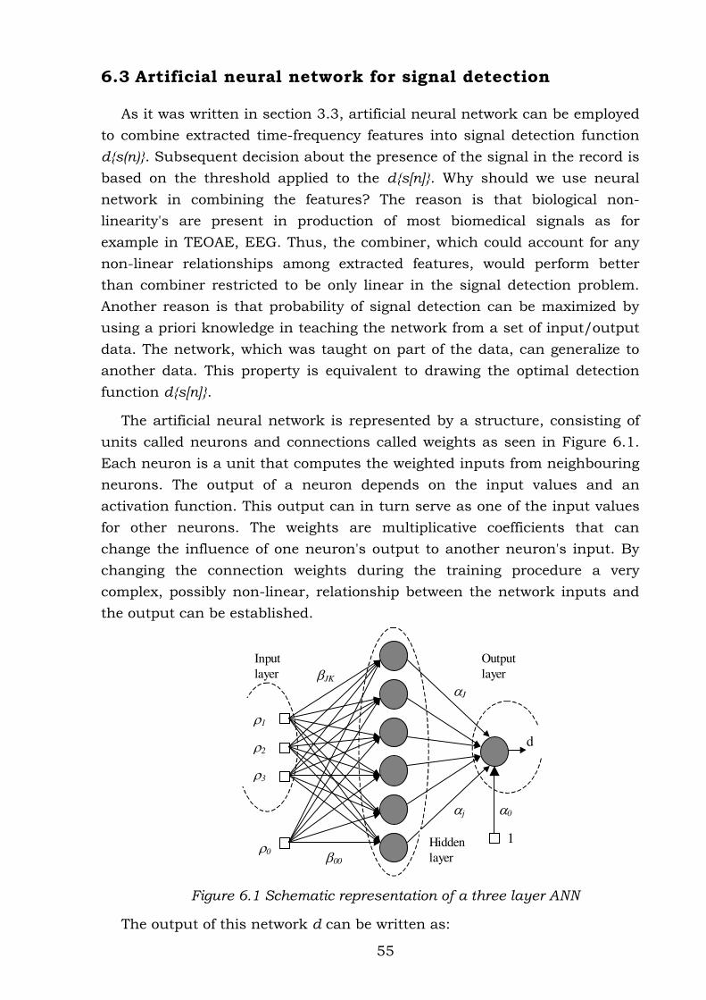
55
6.3 Artificial neural network for signal detection
As it was written in section 3.3, artificial neural network can be employed
to combine extracted time-frequency features into signal detection function
d{s(n)}. Subsequent decision about the presence of the signal in the record is
based on the threshold applied to the d{s[n]}. Why should we use neural
network in combining the features? The reason is that biological non-
linearity's are present in production of most biomedical signals as for
example in TEOAE, EEG. Thus, the combiner, which could account for any
non-linear relationships among extracted features, would perform better
than combiner restricted to be only linear in the signal detection problem.
Another reason is that probability of signal detection can be maximized by
using a priori knowledge in teaching the network from a set of input/output
data. The network, which was taught on part of the data, can generalize to
another data. This property is equivalent to drawing the optimal detection
function d{s[n]}.
The artificial neural network is represented by a structure, consisting of
units called neurons and connections called weights as seen in Figure 6.1.
Each neuron is a unit that computes the weighted inputs from neighbouring
neurons. The output of a neuron depends on the input values and an
activation function. This output can in turn serve as one of the input values
for other neurons. The weights are multiplicative coefficients that can
change the influence of one neuron's output to another neuron's input. By
changing the connection weights during the training procedure a very
complex, possibly non-linear, relationship between the network inputs and
the output can be established.
Inputlayer βJK
β00
αj α0
1
αJ
dρ2
ρ0
ρ1
ρ3
Hiddenlayer
Outputlayer
Figure 6.1 Schematic representation of a three layer ANN
The output of this network d can be written as:

56
⋅⋅= ∑∑
==
J
jjjk
K
kk
tanhtanh),,(d00
ρβαρβα ( 6.10 )
where ρj denotes the feature vector parameters with 10=ρ , J is the
number of inputs, K is the number of hidden neurons, tanh is the non-linear
activation function hyperbolic tangent, βjk are the weights between inputs
and hidden layer and αk are the weights between hidden and output layers.
The neural network training procedure is based on adjusting the weight
parameters αk and βjk. The neural network is considered to be trained when
it gives small errors when applied on the training set of data but also
responds properly to a new testing set not used in the training procedure.
When a network is able to perform both on testing and training sets of data,
we say that the network generalizes well and the optimal detection function
d{s[n]} is established.

57
7 Applications and algorithms
7.1 Wavelet based TEOAE denoising and detection
It is not easy to give the definition of genuine TEOAE response. The large
intersubject variability in the shapes of TEAOE responses do not allow to set
fixed rules for detection and classification of TEOAE’s. For example, we can
see in Figure 7.1 typical TEOAE responses from 4 subjects having similar
MHL about 0dB in 0.5-6.4 kHz frequency band. If we try to compare them
sample by sample, we will not find any similarities among them: at the same
time instances different records have very different values. Although the
TEOAE responses, like fingerprints, can be very stable during long time from
the same ear, but they can be completely different even from the same
subject’s equally hearing left and right ears. Thus global features that
capture similarities in TEOAE responses from similar hearing ears should be
extracted.
Figure 7.1 Examples of TEOAE subaveraged responses from 4 subjects,
having the same MHL ≈ 0dB. Here r indicates cross correlation value between subaverages of the response
We refer to D. Kemp, the first who detected TEOAE in 1978 [47] for
definition of the TEOAE. However, he gives very common definition: “release
or return of acoustic energy from the cochlea into the ear canal, in response
to an acoustic transient”. It was already said that TEOAE responses
distinguish themselves by the signal shape stability for the same subject
during the long time. Thus the most popular criterion for TEOAE detection is
the cross correlation coefficient between the two subaverages (we remind

58
here that TEOAE response is recorded into two accumulators). If the
calculated cross correlation coefficient between the two subaverages exceeds
some predetermined threshold, it is considered as an evidence of the
presence of deterministic activity in the recorded signal and a conclusion
about detected TEOAE is made. The TEOAE responses shown in Figure 7.1
can be clearly distinguished with a high cross correlation value, but this is
not always the case. The calculated cross correlation value depends on both
initial signal-to-noise ratio and available averaging time (i.e. number of
sweeps in the average). Long averaging time is often difficult to maintain in
the clinical practice, especially in child investigations. In order to reduce
further the influence of the remaining noise in the averaged signal,
additional measures can be considered, which use a priori information on
TEOAE. Many investigations [13,10,20] have shown that TEOAE exhibit
frequency dependant latency: where higher frequencies have shorter post-
stimulus time while lower frequencies have longer. This particular feature of
TEOAE can also be observed in the example of TEOAE subaverages shown in
Figure 7.1, where oscillations of higher frequency, starting 3 ms post-
stimulus, precede oscillations with lower frequency. These observations led
us to the assumptions that taking into account such time- frequency specific
structure of TEOAE can increase the signal-to-noise ratio and detection
performance.
As an application of the investigated signal denoising and feature
extraction methods here we present the results of denoising the real TEOAE
signals and automatic TEOAE detection method. The method was
investigated on large database of real TEOAE signals.
7.2 Experimental data
A database consisting of 5213 TEOAE records was collected during the
health screening test "Genetic and environmental study of hearing loss in
Nord-Trondelag county" Norway [24]. The ILO92 Otodynamics analyzer was
used for recording of TEOAE data and air conduction pure tone audiograms
were recorded using Interacoustics AD25 automatic audiometers. The
audiometric criterion used to separate normal hearing from hearing impaired
subjects was chosen as 30 dB of mean hearing level as obtained at the
frequencies 0.5, 1, 2 and 4 kHz (MHL). Based on that separation level a total
of 4404 subjects were classified as having normal hearing while the
remaining 809 were classified as having impaired hearing.

59
7.3 Wavelet based TEOAE denoising
7.3.1 Algorithms
The denoising algorithms described in Sections 5.2.3 and 5.3 were
applied to all the TEOAE records from the database to estimate the efficiency
of proposed methods and to compare them with the methods known from
the literature.
7.3.2 Other methods for signal-to-noise ration improvement in TEOAE records
Various methods have been presented with the aim to improve the SNR
and detection performance of TEOAE, e.g. by time windowing [98] of the
subaveraged signals or by bandpass filtering [34].
Optimal time windowing. Time windowing technique is based on the
assumption that a shorter analysis time window increases the SNR. The best
results were obtained by using the window 2.5-9 ms [98].
Optimal bandpass filtering. In study [34] linear bandpass filtering with
four different octave bandpass filters with center frequencies: 500 Hz,
1000 Hz, 2000 Hz and 4000 Hz were considered to improve SNR. The filter
with central frequency of 4000 Hz gave the best results.
Before processing. The cross correlation coefficient between two
unprocessed subaverages, or "wave reproducibility'", is used as a base for
comparisons. This parameter is used for TEOAE detection in conventional
clinical TEOAE recording device ILO92 manufactured by Otodynamics Ltd.
7.3.3 TEOAE denoising results with different methods
The example of TEOAE record before any processing, after time
windowing, after linear bandpass filtering, after wavelet coefficient shrinkage
based denoising and after wavelet coefficient selection based time- frequency
filtering is shown in Figure 7.2. The cross correlation values reflect the
improvement of the quality of this signal example. Since the mean hearing
level for this particular subject was 10 dB, otoacoustic emissions were
expected to be present. Figure 7.2 shows that no emission is present in the
unprocessed signal (ρ=64 %) as the criterion for the presence of TEOAE is
considered ρ=70 %. All the filtering methods improved ρ in this case and indicated TEOAE signal being present in this record.

60
Figure 7.2 The examples of the TEOAE subaverages: a) before any processing, b) after bandpass filtering, c) after time windowing, d) after
wavelet coefficient shrinkage based denoising, e) after wavelet coefficient selection based time- frequency filtering
It is important to know the influence of the signal denoising procedures
on all the TEOAE records in the database. How differently the different
records with different initial signal to noise ratio were effected by the
denoising procedures? The cross correlation values of unprocessed database,
sorted in ascending order, were chosen as a base for comparison with the
data after denoising. Overall influence of all the denoising methods on all the
signals in the database is shown in Figure 7.3. In the figure the data, cross
correlation values, representing records before denoising are shown as thick
line and the dots correspond to the same sorted subjects after influence of
denoising. It can be observed that all the recordings were affected by the
denoising using time windowing, bandpass filtering, both wavelet based
methods and have spread of cross correlation values in both sides of the
baseline. This means that, in addition, to increased cross correlation values
we get decreased values. The spread of cross correlation values after time
windowing and bandpass filtering is much higher than using wavelet
coefficient shrinkage or coefficient selection based methods. This indicates
less dramatic influence of the last two methods to the signals. Another good
feature of the last two methods is mostly positive direction of the affect to the
records that had cross correlation above some 50% before processing. The

61
records that had before processing the cross correlation value below 40% in
the average were unchanged. It is very important result as it shows that the
denoising procedure will not produce false negatives by discovering TEOAE,
where it should not be.
Figure 7.3 Distribution of cross correlation values computed before and after denoising using: a) time windowing, b), bandpass filtering, c) wavelet coefficient shrinkage, d) wavelet coefficient selection. The line represents the
sorted in ascending order cross correlation values before denoising. The points represent the same signals in the database, but after denoising with different
methods. Here n is the number of the record in the database.
Figure 7.4 gives more insight about the different effect of the denoising
methods to the similar records representing various cross correlation
intervals. It shows the influence of different SNR improvement techniques in
six cross correlation ranges. The recordings were clustered by their cross
correlation value into six groups before application of the processing
techniques. Then all the techniques were applied to the recordings in the
groups and mean cross correlation values calculated. It can be seen that all
the methods, except bandpass filtering, increased the cross correlations in

62
all the selected intervals. The records from the intervals (40-50)%, (50-60)%
and (60-70)% experienced the highest positive influence from both wavelet
based methods, while records from the interval "<30%" are almost
unaffected. Time windowing influenced the records from the all intervals
significantly to the positive direction, too. However, it significantly affected
the records from the interval "<30%", where with high probability only noise
resides. Thus, it is negative feature, since errors (false negatives) can be
produced in signal recognition tasks.
Figure 7.4 Comparison of various SNR improvement techniques in different cross correlation ranges
7.3.4 Discussion
TEOAE signal measurement promises to become a new tool in objective,
quick and reliable assessment of the functionality of inner ear. However,
many problems have to be solved until TEOAE measurement based tests of
hearing will gain the popularity among the clinicians. One of the problems is
a noise reduction or enhancement of the acquired TEOAE signal for reliable
detection.
We have shown that TEOAE signals could be enhanced by using a
knowledge about the time- frequency contents of this kind of signals. The
motivation for this approach was earlier investigations made by Whitehead

63
et.al. [98] and Gorga et.al. [34], where time windowing or bandpass filtering
were used. In contrast, we have tried to use both dimensions: time and
frequency, in signal enhancement. We employed discrete wavelet transform
for mapping the signal into joined time-frequency representation. Discrete
wavelet transform decomposes the signal into octave frequency bands with
increasing time resolution when frequency increases. This property agrees
with time- frequency structure of TEOAE signals, where high frequency
components have shorter duration than low frequency components. Other
authors: Wit et. al. [100] and Tognola et.al. [92], have used continuous
wavelet transform (CWT) for TEOAE analysis. We admit that CWT allows
more flexibility in choosing frequency bands and time resolutions, however it
is highly redundant and computationally expensive. Wavelet pocket analysis
[13] is worth considering. It is an alternative to CWT having some degree of
flexibility in time- frequency plane division and fast analysis algorithms.
The analysis of enhancement of TEOAE signals in database showed
wavelet based algorithm works. These signals, which had very low cross
correlation value (<30 %) before processing, were almost unaffected by the
algorithm i.e. TEOAE was not "found" where it was not present. This is
correct, because it is very high probability that these records were recorded
from impaired ears and contain no TEAOE activity i.e. only noise was
recorded. The group of signals, which had cross correlation value in the
range 40- 70 %, experienced the highest influence (increase of cross
correlation value in the average) by all the signal enhancement methods.
Thus, many previously indeterminate cases, where cross correlation values
were just below the decision threshold of 70 %, reached the threshold and
can be diagnosed as normal hearing. However, these signals may represent
either TEOAE signals, which are contaminated by high amplitude subject
generated and environmental noises, or pure noise, which has accidentally
achieved high cross correlation value. The question arises: which signals
were enhanced more in this group? There could be two possible answers to
this question: a) just signals having TEOAE activity were enhanced, b) both
types of signals with TEOAE activity and without it were enhanced equally.
The first possibility is desirable as the number of subjects that were miss
classified as hearing impaired would decrease, while the second would bring
highly undesirable consequences: hearing impaired subjects might be
diagnosed as normal hearing. We will try to answer the former question in
the next section where the detection of TEOAE or classification of subjects
into normal hearing and hearing impaired will be considered.

64
7.4 TEOAE feature extraction and detection
As it was written in section 7.1, the features that take into account
specific time-frequency properties of TEAOE can be more useful than, for
example, gross features like energy or maximum amplitude of the signals.
Thus, feature extraction procedure, which was described in section 6 was
used in our TEOAE feature extraction problem.
Choosing wavelet coefficients from decomposition level j is equivalent to
bandpass filtering of the signal, while choosing wavelet coefficients with
indexes from k to l from the given decomposition level is equivalent to time
windowing. The fast orthogonal discrete wavelet transform decomposes the
signal by definition into octave frequency bands, which cannot be chosen
independently. The time windowing in wavelet domain can, however, be
accomplished with no restriction in the choice of the indexes k and l.
The choice of time indexes k and l in our TEOAE specific feature
extraction problem was based on the data from the section 5.3, where the
average location of the bigger part of the TEOAE energy in the selected levels
was determined. Our data agrees with data from a study of Janušauskas et.
al. [40], where the average time locations of TEOAE in a database of normal
hearing subjects was studied by the use of an ensemble correlation
technique. The time windowing was thus carried out directly in wavelet
domain by selecting or, equivalently, by applying the rectangular windows to
the wavelet coefficients from the given level of decomposition (as seen in
Figure 7.5). The features, cross correlation coefficients between two
windowed frequency components of two TEOAE subaverages A and B in the
wavelet domain, are then obtained as:
( ) ( )
( ) ( )
22 ∑∑
∑
==
=
⋅
⋅=
l
kn j,Bl
kn j,A
l
kn j,Bj,A
jnwnw
nwnwρ ( 7.1 )
where wA,j and wB,j are wavelet coefficients of subaverages A and B from
level j and where k and l are indexes of the first and last coefficient in the
respective window.
An example of TEOAE subaverages transformed into wavelet domain is
shown in the Figure 7.5. It can be seen that the highest similarity between
the wavelet coefficients and equivalently the highest cross correlation
appears in rectangular windows as defined by Janušauskas et. al. The
calculated cross correlation values between the TEAOE subaverages with

65
and without windows, as indicated in the Figure 7.5, exemplify the
improvement achieved by windowing.
Figure 7.5 Three levels of wavelet decomposition of two subaverages and corresponding time windows. The two subaverages A and B are shown as open and filled circles, respectively. Solid lines indicate corresponding time
windows ( k is time index ). The cross correlation values ρj with and without windows (in parentheses) are indicated.
The three cross correlation coefficients ρj, which represent each recorded signal consisting of two subaverages with 512 time samples each are in the
following used as TEOAE features.
7.4.1 Feature average based detector
In order to establish TEAOE detection criterion, features extracted from
recorded signals should be combined in some way to form the detection
function d{s[n]}. The final decision, about the presence of TEAOE in the
response can be made by setting the threshold on the value of detection
function. Two ways to combine the features in order to form d{s[n]} for
TEAOE detection were proposed.
The first detection function was constructed as simple feature average.
This assumes that extracted features, time and frequency limited cross
correlation coefficients, have equal weights in forming discriminatory
function to detect TEOAE:

66
ρρρρρρ 321321 31
31
31 ++=),,(d ( 7.2 )
In addition, we associate the presence of TEOAE with normal hearing
(mean hearing threshold less than 30 dB). Thus, separation of subjects
belonging to normal hearing or hearing impaired is made according to this
rule:
T
IH
NH
),,(d <≥=321 ρρρ ( 7.3 )
where NH represents the normal hearing subjects, IH the impaired
hearing subjects, T is the threshold value.
7.4.2 Neural network based detector
It is well known that TEOE generation is closely related with non-
linearities which are present in the cochlea and which are responsible for the
high dynamic range of the hearing system. Thus, it would be natural to
think about more complex relationship than linear in associating hearing
level and time-frequency features extracted from TEOAE. Artificial neural
networks are used in applications, where predetermined analytical
relationships are difficult to establish because of the lack of knowledge about
the phenomenological background, but where rich empirical datasets are
available for teaching of the network of the desired relationship. Thus, we
were inspired by our large database of TEOAE records to construct the
second TEOAE detection and subject separation parameter with the help of
artificial neural network.
The multilayer perceptron was chosen due to its ability to model both
simple and very complex functional relationships [14]. We restricted,
however, ourselves to consider artificial neural network having only one
hidden layer and only hyperbolic tangent activation functions. The Bayesian
technique of regularization proposed by D. Foresee and F. Hagan [29] to
improve generalization was used in training procedure. In addition, this
regularization procedure gives the number of weights in the neural network
that are effectively used in reducing the error function. This feature can be
employed to choose optimal number of network neurons. We can simply add
more neurons and retrain. If the larger network has the same final effectively
used number of parameters, then the smaller network was large enough. In
our case, the final network had 3 inputs, 6 neurons in the hidden layer and

67
one neuron in the output layer. The weights were adjusted using Levenberg-
Marquardt algorithm during the training procedure. This algorithm has the
most rapid convergence properties for networks with moderate
complexity [37].
The network was trained using supervised learning with a training set of
inputs and targets. This procedure is described by:
dBMHL
dBMHL
if,
if, ),,(d
3030
11
221 ≥<
−=ρρρ ( 7.4 )
where d(ρ1, ρ2, ρ3) is the detection function, which has to be determined
by the ANN to minimize the mapping error of the features ρ1, ρ2, ρ3 to the targets, the binary values 1 and –1. These binary values represent the
subjects having audiometric MHL in frequency range 500-4000 Hz less than
30 dB and more than 30 dB, respectively. Thus, normal hearing subjects are
coded by “1” and hearing impaired subjects by “-1”.
The preliminary attempts of the neural network training showed that the
network generalized well if the training set consisted of approximately equal
number of hearing impaired and normal hearing cases. The training set was
therefore made of a database representing 385 hearing impaired and 400
normal hearing subjects. The testing set contained all the subjects: 809
hearing impaired and 4404 normal hearing.
The separation of subjects belonging to one of the groups is made
according to the rule in ( 7.3 ).
7.4.3 Statistical decision theory for the comparison of the detectors
The principles of statistical decision theory [67] were used for the
comparison of the different detectors. The ROC curves (introduced in
section 3.3) were used to assess the ability of the detectors to detect TEOAE
signals.
In TEOAE detection applications it is important to have high sensitivity of
the detector to identify the main part of the hearing impaired subjects. The
comparison of the performance of the different detectors was therefore made
by keeping the sensitivity at a fixed level of 90 % and comparing the
resulting specificity.

68
7.4.4 Subject separation results when separation parameter is an average of the features extracted from TEOAE
In order to validate the increased complexity of the new denoising
methods, comparison with conventional TEOAE detection techniques, which
were described in section 7.3.2 as noise reduction techniques, was made.
The detection function d(ρi) was: the average of the three cross correlation coefficients in case of wavelet based time- frequency feature extraction
"Time- frequency feat." method and the simple cross correlation coefficient in
the remaining methods.
Figure 7.6 shows fife ROC curves corresponding to different methods of
TEOAE signal processing and feature extraction.
Figure 7.6 ROC curves before any processing of TEAOE signals ("Before process."), after windowing ("Opt. time wind."), after linear bandpass filtering ("Opt. bandpass filt."), after non-linear wavelet based filtering ("Wavelet coef. shrink.") and after wavelet based time- frequency feature extraction ("Time-
frequency feat.")
It was shown that wavelet methods and especially wavelet based time-
frequency feature extraction method outperform the other methods by
achieving a better specificity at all investigated sensitivity value. The
specificity values at a sensitivity of 90 % are presented in Table 7.1

69
Table 7.1 The specificity of different TEOAE detection methods at 90% of sensitivity
Method Used signal features
Specificity±std,
(Sensitivity=90%)
Before processing ρ [68,03±0,70] %
Time windowing
(∆t=(2.5-12,5)ms). ρ [72,31±0,67] %
Bandpass.filt.
(∆f=(2-4)kHz) ρ [78,12±0,62] %
Wavelet coef. shrinkage
ρ [79,51±0,61] %
Time frequency features
ρ1, ρ2, ρ3 [82,71±0,57] %
In order to provide further insight into the above results, the sensitivity
and the specificity are presented separately as the decision threshold
functions1 in Figure 7.7. Again, it is obvious that time windowing
corresponds to a less favourable sensitivity and specificity than do the
wavelet methods. Bandpass filtering has a better sensitivity but a worse
specificity than the other methods; the sensitivity characteristic is explained
by lower noise contamination in the higher frequency region which reduces
the likelihood of high cross correlation values due to correlated noise
artefacts.
1 A sensitivity curve, which is less steep indicates that, for a certain value of the
separation parameter, a larger number of cases are mistaken as true OAE as a consequence of residual stimuli or correlated noise artifacts. A specificity curve, which is less steep indicates a larger number of cases where noise is insufficiently reduced or where an OAE was not present because of methodological problems.

70
Figure 7.7. Sensitivity and specificity versus threshold.
7.4.5 Comparison of linear and non-linear TEOAE detectors in hearing screening
In order to check if more complex detector than linear can perform better
in separation normal hearing subjects from those with hearing loss we
compared two detectors. The first used simple average of features as
separation parameter and the second neural network, which can combine
extracted features, in such a way as the best separation performance could
be achieved. Both classifiers, the linear and the non-linear, transformed a
vector of three TEOAE features, representing one subject, into one single
output. The results of both classifiers are shown in Figure 7.8 and Figure
7.9. Normal hearing subjects are grouped in the left part of the figures (4404
subjects), while hearing impaired are grouped in the right part (809
subjects). The decision threshold (dashed horizontal line) for separation of
hearing impaired from normal hearings is selected such that sensitivity of
90 % is obtained. It can be observed that most of normal hearing subjects
are above the decision threshold. They constitute the true negatives. The
normal hearings below the decision threshold are the false positives.
Similarly, hearing impaired subjects (right side of the graphs) below the
threshold are true positives and above the threshold are the false negatives.
It can be concluded that the linear approach distributes subjects more
evenly in comparison with ANN, which seems to separate most of subjects in
two distant regions. Although, this looks like an advantage of the non-linear

71
approach versus linear, the improvement expressed as a specificity value is a
minor showing a difference between the methods of 82.7 % versus 84.1 % for
a specificity at a sensitivity of 90 %. The numbers of correctly and not
correctly identified subjects and the calculated 95 % confidence intervals of
specificity at 90 % of sensitivity for both types of classifiers are presented in
Table 7.2.
Figure 7.8 Separation of normal hearing and hearing impaired subjects
using a linear classifier. Here ρ is the average of the features- ρ1, ρ2 and ρ3
Figure 7.9 Separation of normal hearing and hearing impaired subjects using ANN separation

72
A comparison of the numbers of false negatives and false positives shows
close similarity between the classifiers with minor improvement for the non-
linear classifier, which gives less number of false positives (Table 7.2).
Table 7.2 The separation results at 90% of sensitivity
NT TP FN FP Specificity and std.
Confidence interval (0.05%)
Linear classif.
3644 727 82 760 (82.7±0.57) % [81.6– 83.8]%
Non-linear classif.
3704 726 83 700 (84.1±0.55) % [83- 85.2]%
It may be assumed that larger differences would appear at other levels of
sensitivity. But this is not the case, as can be seen in the ROC curves in
Figure 7.10. The curves indicate that the separation methods are very
similar, though, non-linear approach exceeds linear at several regions.
Figure 7.10 ROC curves for both methods
Although the resulting difference between the two methods was small, we
could prove that the difference is statistically significant by applying a
hypothesis test with the null hypothesis defined, as "no differences among
the results from the classifiers". After making the assumption about normal

73
distribution of the results, the hypothesis test showed that we could reject
the null hypothesis, as the evaluated P value was 0.0002.
The dependence of separation accuracy in terms of sensitivity and
specificity curves as the functions of decision threshold is shown in Figure
7.11. Before comparison, outputs of the neural network were transformed
into the same range as averaged cross correlation values: from 0 to 100 %.
The curves show that to achieve the same sensitivity of 90 % different
decision thresholds should be applied: 70 % for linear method and 53 % for
non-linear. The shapes of the curves from respective method differ
considerably for a given decision threshold value; the difference is
particularly large between the sensitivity curves. This is due to
transformation of distribution of hearing impaired subjects by the non-linear
classifier as it shown in Figure 7.8 and Figure 7.9.
Figure 7.11 Sensitivity and specificity of linear and non-linear classifiers as the functions of the separation threshold.
7.4.6 Discussion
In this section we compared different signal processing methods to
increase accuracy of the separation hearing impaired and normal hearing
subjects in the database using TEOAE records. The question, which was left
from the section 7.3 can be answered. The question was: which signals were
enhanced more in the group of signals that have cross correlation value just
below the threshold? There were two possible answers to this question: a)
just signals having TEOAE activity were enhanced, b) both types of signals
with TEOAE activity and without it were enhanced equally. Now we can

74
answer from Table 7.1 that signals having TEOAE activity were enhanced
more, since the accuracy of subject separation was improved.
Further, we compared two classifiers to separate hearing impaired and
normal hearing subjects, using TEOAE based features. The first classifier
was constituted by the linear average of the set of features, while the second
one- based on neural network, which could account for a more complex
relationship, possibly non-linear, among the set of features as extracted from
TEOAE and the mean hearing level in the frequency range 0.5-4 kHz. Based
on the facts about non-linear TEOAE generation mechanism in the cochlea
we expect a substantial improvement in subject separation using more
complex non-linear classifier as compared to a linear. The results were,
however, very similar with a small but still statistically significant advantage
of the neural network based classifier.
A possible reason why the neural network did not decrease the number of
errors might be due to the fact that the database includes a certain amount
of errors caused by deficient measurements of TEOAE or audiograms. The
outliers may prevent the neural network from the establishment of the right
separation function during the training procedure. We have manually
inspected some cases with erroneous behaviour: hearing impaired subjects
with a TEAOE like response (false negatives) and normal hearing subjects
with a response in which TEOAE cannot be detected (false positives). There
are several reasons that may contribute to false positives: a) poor fitting of
the probe into the ear canal (loose seal to the ear canal reduces stimulus
pressure and TEOAE amplitudes), b) a blockage of the microphone or
speaker ports against the ear canal wall or by ear wax, which prevents the
recording of the TEOAE response, c) strong ambient noise during the session
of recording, d) conductive hearing loss in middle ear from 10 to 20 dB can
make emission undetectable. One example of a false positive case is shown
in Figure 7.12, where the subject has MHL=4 dB indicating the potential to
generate TEAOE and where the ρ value equal to 40 % indicates mainly the
random activity. The possible reasons for low ρ value might be a) somewhat
low stimulus pressure –72 dB (scaled stimulus is shown in the left-hand side
of the figures), while the average pressure is 80 dB in the database and b)
strong ambient noise.

75
0 5 10 15 20
-6
-4
-2
0
2
4
6
8
x 10 -5
Pre
ssu
re,
Pa
Time, ms
ρ =40%, MHL = 4dB
Figure 7.12 The example of TEOAE response in case of false positive subject
False negatives, may also appear due to technical failures: a) bad fitting of
the probe into the ear canal may cause prolonged stimulus artefact, which
will give increased cross correlation values, b) noise from instrumentation
which is synchronized with stimulus may be detected as the TEOAE.
0 5 10 15 20
-2
-1.5
-1
-0.5
0
0.5
1
1.5 x 10
-4
Pre
ssu
re,
Pa
Time, ms
ρ =66%, MHL = 39dB
Figure 7.13 An example of prolonged artifact
Figure 7.13 shows an example representing a false negative case, which
may have increased cross correlation value due to prolonged stimulus
artefact. This subject is classified as normal hearing although the MHL is
39 dB.
It is, however, sometimes difficult to find a simple explanation for the
achieved error. Figure 7.14 shows a TEOAE response from a subject, which
is hearing impaired according to audiometric data with MHL 53 dB.

76
0 5 10 15 20
-2
-1
0
1
2
x 10 -4
Pre
ssu
re,
Pa
Time, ms
ρ =93%, MHL = 53dB
Figure 7.14 The example of false negative case
This response looks like a response from a completely normal hearing
subject, where: high, middle and low frequencies easily can be distinguished
in the response. One possible explanation for this example is that it may be
a retrocochlear hearing loss, which means that the hearing loss is caused by
dysfunction the auditory pathway after the cochlea. Such a condition cannot
be detected by a TEOAE test, since these cases have a normal cochlea
producing a normal TEOAE. Another possible explanation is error in the
measurement of the audiogram.

77
8 Conclusions
The following conclusions can be derived from this study:
1. Signal denoising in the transform domain can be more effective than
in the original time domain. We showed that the energy of the non-
stationary signal is concentrated better in discrete wavelet domain
than in discrete Fourier domain or time domain.
2. We found that among the families of finite in time and orthogonal
wavelets: Daubechies2-20, Coiflet1-5, Symmlet2-10, the best
performance in terms of energy concentration showed Symmlet 8
wavelet.
3. We proposed two different algorithms to enhance the signal in
wavelet domain. One of them is based on wavelet coefficients
thresholding and we proposed the method to estimate the threshold,
which maximizes the quality of the signal. Other algorithm uses
knowledge about average location of signal components in wavelet
domain for relevant wavelet coefficients selection. These methods
were compared with other wavelet based denoising methods in the
problem of TEOAE signal enhancement. The results showed that
method based on wavelet coefficient selection is the best among
compared methods and could reduce averaging time needed to
achieve the signal of sufficient quality. The quality of enhanced
signal averaged over 16 realizations was approximately equal to
unprocessed signal, which was averaged over 60 realizations.
4. Signal denoising method based on wavelet coefficient selection was
validated in the application of denoising 5213 TEAOE signals from
large database. The results showed that processing mainly affects
these signals, which have average quality in the beginning. This is an
important property as no clean signal is produced from noise only.
5. In the problem of signal detection, we proposed the efficient
procedure to extract features from the non-stationary signal. We
showed that calculation of band limited product of two signals in
time is equivalent to the calculation directly in wavelet domain.
Furthermore, windowing in time can be replaced with selection of
relevant wavelet coefficients. Thus, calculations of cross correlation
coefficients between time and frequency limited intervals of two
signals can be accomplished very efficiently in wavelet domain.

78
6. The algorithm for automatic separation of hearing impaired and
normal hearing subjects using the features extracted from TEOAE
signals was proposed and tested on the database of 5213 signals. By
using proposed features, the specificity of separation was increased
by 10-15 % in comparison with conventional features.
7. We compared two classifiers in separation of hearing impaired and
normal hearing subjects, using TEOAE based features. The first
classifier was constituted by the linear average of the set of features.
The second classifier was based on neural network, which could
account for a more complex relationship, possibly non-linear, among
the set of features as extracted from TEOAE and the mean hearing
level in the frequency range 0.5-4kHz. We expected, based on the
facts about non-linear TEOAE generation mechanism in the cochlea,
a substantial improvement in subject separation using more complex
non-linear classifier as compared to a linear. The results were,
however, very similar with a small but still statistically significant
advantage of the neural network based classifier.

79
Acknowledgements
I would like to thank my supervisor Dr. Arūnas Lukoševičius for his
valuable advice, guidance and encouragement over the past five years. I
would also like to thank other two my supervisors: Lic. Owe Svensson and
Dr. Leif Sörnmo for many interesting discussions, proof reading research
papers and hospitality in Lund university and at Bengt Lidfors vägen.
I also want to thank Dr. Bo Engdahl from Dept. of Environmental
Medicine, National Institute of Public Health, Oslo, Norway for providing the
TEOAE signals and consultations.
Thanks to my colleague and friend PhD student Artūras Janušauskas for
all the hot discussions. Thanks to my friends PhD students Rytis Jurkonis
and Vytautas Petkus, who helped to refresh my minds.
Last but not least, I would like to give my special thanks to my wife, Alma.
This work was supported by Swedish Institute and Lithuanian Sciences
and Studies Fund.

80
Bibliography
[1] Abbate A., Koay J., Frenkel J., Schroeder S. C., Das P.. “Signal Detection and Noise Suppression Using a Wavelet Transform Signal Processor: Application to Ultrasonic Flaw Detection”, IEEE Transactions on Ultrasonics, Ferroelectrics, and Frequency Control, Vol. 144, No. 1 January 1997.
[2] Allen J. B. “Cochlear modelling,” IEEE ASSP Magazine , Vol. 2, pp. 3-29, 1985.
[3] Altman D.K. "Practical Statistics for Medical Research", Chapman & Hall, Edinburgh, 1992
[4] Atarius R. Sörnmo L. "Signal to noise ratio enhancement of cardiac late potentials using ensemble correlation" Transactions on biomedical engineering , vol, 42 No.11, 1995.
[5] Axmon J. "Noise suppression using the discrete wavelet transform" Master thesis, Lund university, 1997.
[6] Bray P.J. Click evoked otoacoustic emissions and the development of a clinical otoacoustic hearing test instrument. - PhD thesis, University of London. 1989.
[7] Bruce A., Gao H. “Wave Shrink: Shrinkage functions and thresholds” StatSci Division, MathSoft, Inc.
[8] Buller G., Lutman M.E. “Automatic classification of transiently evoked otoacoustic emissions using an artificial neural network”, British Journal of Audiology, 32, pp.235-247, 1998.
[9] Chan Y.T. “Wavelet basics”, Kluver Academic Publishers, 2nd print., 1995.
[10] Cheng J. "Time-frequency signal representation of transient evoked otoacoustic emissions via smoothed pseudo Wigner distribution" Technical report, ISSN 0280-6819 TA129, 1993.
[11] Ciaccio E.J., Dunn S.M., Akay M. "Biosignal pattern recognition and interpretation systems" IEEE engineering in medicine and biology, Sept., pp.89-95,1993
[12] Cody M. A. “The Wavelet Packet Transform Extending The Wavelet Transform” Dr Dobb’s Journal, April,1994
[13] Cohen A., Kovaèevic J. “Wavelets: The Matematical Background” IEEE Proceedings Of The IEEE vol 84, No.4. April 1996.
[14] Cohen L. “Time- Frequency Analysis”, Prentice Hall, Englewood Cliffs, 1995.

81
[15] Crutchfielfd J.P. "Information and its metric" Published in "Non-linear structures in physical systems- pattern formation, chaos and waves" L. Lam and H.C. Morris, Springer-Verlag, New York, pp.119-130, 1990.
[16] Daubechies I. Ten Lectures on Wavelets. - SIAM, 1992.
[17] Donoho D. L. "De-noising by soft-thresholding", Transactions on information theory, 41(3), pp.613-627 1995.
[18] Donoho D. L. and Johnstone I. M. "Adapting to Unknown Smoothness Via Wavelet Shrinkage", J. Am. Statist. Ass., 90, pp.1200-1224, 1995.
[19] Donoho D. L. and Johnstone I. M. "Minimax Estimation via Wavelet Shrinkage", Technical report Nb. 402, Stanford University, 1992.
[20] Donoho D. L. Non-linear Wavelet Methods for Recovery of Signals, Densities, and Spectra from Indirect and Noisy Data, Proceedings of Symposia in Applied Mathematics, pp.173-205, 1993.
[21] Donoho D.L., Johnstone I.M., Kerkyacharian G. and Pickard "Wavelet shrinkage: Asymptopia?" J. R. Statist. Soc. B, 57 (2), pp. 301-337, 1995.
[22] Durka J. “Time frequency analyses of EEG”, PhD dissertation, 1996.
[23] Engdahl B. “Clinical applications of otoacoustic emissions”, Ulleval University Hospital, Oslo, 1996.
[24] Engdahl B. “Otoacoustic emissions in general adult population I: Age, gender and ear side.” Submitted.
[25] Engdahl B., Tambs K., Borchgrevnik H., Hoffman H. “Otoacoustic emissions in general adult population II: Pure tone hearing thresholds.” Submitted
[26] Engdahl B., Woxen O., Arnesen A.R., Mair I.W. “Transient evoked otoacoustic emissions as screening for hearing losses at the school for military training”, Scand. Audiology, 25, pp. 71-78, 1996.
[27] Flanagan, J.L. Speech analysis, synthesis and perception, 2nd ed., Springer- Verlag, New York, NY, 1972.
[28] Flandrin P. “On Time- Frequency and Wavelet methods”, Medical &Biological Engineering & Computing Vol. 34, Supplement 1, Part 1, 1996
[29] Foresee D., Hagan F. “Gauss-Newton approximation to Bayesian learning” International Conference on Neural Networks, 1997, Volume: 3, pp. 1930 -1935, 1997.

82
[30] Giguere, C. and Woodland, P.C. “A computational model of the auditory periphery for speech and hearing reserch.I.Ascending path,” J. Acoust. Soc. Am. 95, 331-342, 1994.
[31] Glasberg B.R. and Moore B.C.J. “Derivation of auditory filter shapes from notched-noise data.”Hearing Research, vol. 47, 1990, pp. 103-108.
[32] Gold T. Hearing II. The physical basis of the action of the cochlea. Proceedings of the Royal Society B, 135:492- 498, 1948.
[33] Goldstein J.L. “Relations among compresion, suppresion and combination tones in mechanical responses of the basilar membrane: data and MBPNL model” Hearing Research 89, 52-68, 1995.
[34] Gorga M.P., Neely S.T., Bergman B.M., Beauchaine K.L., Kaminski J.R., Peters J., Schulta L. and W. Jesteadt "A comparison of transient-evoked and distortion product otoacoustic emissions in normal- hearing and hearing- impaired subjects" J Acoust Soc Am. (94), pp.2639-2648, 1993.
[35] Grandori F., Cianfrone G. and Kemp D.T., "Cochlear mechanisms and otoacoustic emissions" Adv. Audiol. vol. 7, pp. 99-109. 1990.
[36] Greenwood D. D., “A cochlear frequency-position function for several species—29 years later,” Journal of the Acoustical Society of America, Vol. 87 (6), June 1990, pp. 2592-2605.
[37] Haykin S. “Neural networks. A comprehensive foundation”, Prentice- Hall, 1994.
[38] Hero A. "Signal detection and classification" Internal report, University of Michigan, 1998.
[39] Hussain D.M., Gorga, M.P., Neely, S.T., Keefe, D.H. and Peters, J "Transient evoked otoacoustic emissions in patients with normal hearing and in patients with hearing loss" Ear Hear 19, 434-449, 1998.
[40] Janušauskas A., Engdahl B., Svensson O. and Sörnmo L. “Latency of otoacoustic emission frequency components”, in proc. of 11th Nordic-Baltic Conference on Biomedical Engineering, Tallinn, Estonia, pp.332-334, 1999.
[41] Janušauskas A., Marozas V., Engdahl B., Svensson O. and Sörnmo L."Otoacoustic emissions and improved pass/fail separation using wavelet based denoising", in proc. of 20th Annual International Conference of the IEEE Engineering in Medicine and Biology Society, Hong Kong, pp.3129- 3131, 1998.
[42] Johnsen N.J., Bagi P., Elberling C., Parbo J. "Evoked acoustic emission: clinical application" Acta Otolaryn., pp. 77-85. 1985.
[43] Johnstone I. M. and Silverman B. W. "Wavelet threshold estimators for data with correlated noise" Tech. Report, University of Bristol, UK, 1994.

83
[44] Kapadia S., Lutman M.E. “Are normal hearing thresholds a sufficient condition for click- evoked otoacoustic emissions?” J.Acoust.Soc.Am., vol.101, no.6, pp.3566-3576, 1997.
[45] Kemėšis P., Stasiūnas A. “Žmogaus klausos analizatoriaus savybių modeliavimas”, Biomedicininė inžinerija- 98., KTU, 1998.
[46] Kemėšis P., Stasiūnas A., Kemėšis P. “Akustinio proceso daugiamatis modelis”. Automatika ir valdymo technologija- 98., KTU, 1998.
[47] Kemp D. T. Stimulated acoustic emissions from within the human auditory system. Journal of the Acoustical Society of America, 64:1386-1391, 1978.
[48] Kemp D. T., Bray P. “Hearing faculty testing”, United States Patent 4.884.447, 1989.
[49] Kemp D.T. Rayn S. “Otoacoustic emission tests in neonatal screening programs”, Acta Otolaryngol. (Stockh.) Suppl.482, pp.73-84, 1991.
[50] Kemp D.T., Ryan S. and Bray P. "A guide to effective use of otoacoustic emissions" Ear. Hear., vol. 11, no. 2, pp. 93-105. 1990.
[51] Kemp D.T.. "Stimulated acoustic emissions from within the human auditory system" J. Acoust. Soc. Am., vol. 64, no. 5, pp. 1386-1391. 1978.
[52] Lim, J.S. Two dimensional signal and image processing, Prentice Hall, Englewood Cliffs, NJ, 1990.
[53] Lutman M.E. "Evoked otoacoustic emissions in adults: Implications for screening" Audiol. Pract., vol. 6 (3), pp. 6-8. 1989.
[54] Lutman M.E."Reliable identification of click - evoked otoacoustic emissions using signal - processing techniques" British J. Audiol., vol. 27, pp. 103-108. 1993.
[55] M.L.Whitehead, A.M.Jimenez, B.B.Stagner, M.J. McCoy, B.L.Lonsbury-Martin, and G.K.Martin. "Time windowing of click evoked otoacoustic emissions to increase signal-to-noise ratio," Ear Hear., vol.16, pp.599-611, 1995.
[56] Mallat S. "Wavelet tour of signal processing", Academic Pres, 1998.
[57] Mallat S.. "Multiresolution aproximation and wavelets" Trans. Am. Math. Soc., vol. 315, pp. 69-88. 1989.
[58] Marozas V., Janušauskas A., Engdahl B., Svensson O. and Sörnmo L. “Detection of Otoacoustic emission in the wavelet domain”, in proc. of 11th Nordic-Baltic Conference on Biomedical Engineering, Tallinn, Estonia, pp.334-335, 1999.

84
[59] Marozas V., Janušauskas A., Lukoševičius A. “Oto Akustinės Emisijos (OAE) Fenomenas. Metodas OAE signalø charakteristikai.” Proceed. of conf. “Biomedical engineering”, 1997.
[60] Meddis R., Hewitt M., J. “Virtual pitch and phase sensitivity of a computer model of the auditory periphery. I: Pitch identification” J. Acoust. Soc. Am. 89, 2866- 2882, 1991.
[61] McFadden D. and Pasanen G. E. “Otoacoustic emissions and quinine sulphate” J. Acoust. Soc. Am., 95(6):3460-3474, 1994
[62] Morgan D. P. and Scofield C. L Neural Networks and Speech Processing Kluwer Academic Publishers, Boston, MA1991.
[63] Muller K. and Stephan K. "Confirmation of transiently evoked emissions based on user independent criteria," Audiol., vol. 33, pp. 28-36. 1994.
[64] Neely S.T., Norton S.J., Gorga M.P. and Jesteadt. "Latency of auditory brain stem responses and acoustic emissions using tone - burst stimuli" J. Acoust. Soc. Am.., vol. 83, no. 2, pp. 652-656. 1988.
[65] Newland D.E.”An introduction to random vibrations, spectral and wavelet analysis”, Longman Pub Group, 1993.
[66] Nguen T., Strang G.. Wavelets and Filter Banks. Wellesley-Cambridge Press, 1996.
[67] Nielsen N. H., Wickerhauser M. V. “Wavelets and Time-Frquency Analysis”. IEEE Proceedings Of The IEEE vol 84, No.4. April 1996.
[68] Nielsen W., Turner R.G. "Application of clinical decision analysis to audiological tests" Ear. Hear., pp. 125-133. 1984
[69] O’Mard L. P., Meddis R. “A computational model of non- linear auditory frequency selectivity”,
[70] O’Mard L. P., Meddis R. “Dual Resonance Non-linear Filter Model (DRNL)”, http://www.essex.ac.uk/psychology/hearinglab/projects/projects.html
[71] Ozdamar O., Zhang J., Kalayci T., Ulgen Y. "Time- frequency distribution of evoked otoacoustic emissions" British Journal of Audiology , pp. 461-471, 1997.
[72] Pasanen E.G., Travis J.D. Thornhil R.J. "Wavelet-type analysis of transient-evoked otoacoustic emissions" ISA, pp.75-80, 1994.
[73] Patterson R.D. Robinson K., Holdsworth J., McKeouwn D., Zhang C., and Allerhand M., "Complex sounds and arbitrary images" In: Y. Cazals, L. Demany and K. Horner , Auditory physiology and perception, Pergamon Eress, Oxford, pp. 429-446,1992.

85
[74] Prieve B.A. "Click and tone-burst-evoked otoacoustic emissions in normal and hearing-impaired ears" J.Acoust.Soc.Am., vol.99, no.5, pp.3077-3086, 1996.
[75] Prieve B.A.. "Click and tone-burst-evoked otoacoustic emissions in normal and hearing-impaired ears" J. Acoust. Soc. Am., vol. 99, no. 5, pp. 3077-3086. 1996.
[76] Probst R. "A review of otoacoustic emissions" J. Acoust. Soc. Am., vol. 89, no. 5, pp. 2027-2067. 1991.
[77] Rahko T., Kumpulainen P., Ihalainen H., Ojala E., Aumala O. "A new analysis method for the evaluation of transient evoked otoacoustic emissions" Acta Otolaryngol. (Stockh), Suppl. 529, pp.66-68, 1997.
[78] Ravazzani P., Tognola G., Grandory F. "Optimal band passfiltering of transient evoked otoacoustic emissions in neonates" Audiology 38, pp.69-74, 1999
[79] Riol O., Flandrin P. “Time-Scale Energy Distributions: A General Class Extending Wavelet Transforms” IEEE Transactions on Signal Processing vol 40, No.7. July 1992.
[80] Robert A., Ericsson "A composite model of the auditory periphery for simulating responses to complex sounds" J. Acoust. Soc. Am., 106 (4), pp. 1852-1864, 1999.
[81] Robini M.C., Magnin I.E., Benoit-Cattin H., Baskurt A. “Application On The Wavelet Packet Tranform To Flow DetectionIn Ultrasound B-Scans” 1995 IEEE Ultrasonics Symposium
[82] Ruskai M.B. “Wavelets and their applications”, Jones and Bartlet Pub. 1992.
[83] Slaney M. “An Efficient Implementation of the Patterson-Holdsworth Auditory Filter Bank”, Apple Computer Technical Report #35 Apple Computer Corporate Library, Cupertino, CA 95014, 1993.
[84] Slaney M. “Lyon’s Cochlear Model,” Apple Technical Report #13, Apple Computer Corporate Library, Cupertino, CA 95014, 1988.
[85] Strand F. L. “Physiology: a regulatory systems approach”, Macmilian Publishing Co., Inc., New York, 1978.
[86] Strang G. Nguyen T. "Wavelets and filter banks" Wellesley- Cambradge Press, 1996
[87] Sveldens W. “Wavelets: what next?”. IEEE Proceedings Of The IEEE vol 84, No.4. April 1996.
[88] Svensson Owe "Estimation of evoked potentials" Sig. Proc. Rep. SPR-12, Lund 1991
[89] Therrien C. "Discrete random signals and statistical signal processing" Prentice Hall, 1992

86
[90] Tognola G., Borella G. and Grandori F. "Filtering techniques for the analysis of otoacoustic emissions" Submited to Proc. 13th South. Biomed. Eng.. 1994.
[91] Tognola G., Grandori F., Ravazzani P. “Latency distribution of click-evoked otoacoustic emissions” in Proc. 1996 IEEE Eng. Med. Biol., Amsterdam, the Netherlands, 1996.
[92] Tognola G., Grandori F., Ravazzani P. “Time- frequency distributions of click- evoked otoacoustic emissions”, Hearing Research (1997) 1-11.
[93] Tognola G., Ravazzani P. and Grandori F. "Reduction of low-frequency noise in click evoked otoacoustic emissions. An optimal filtering approach" IEEE Trans. Biomed. Eng., pp. 1302-1304. 1994.
[94] Ueda H. "Do click- evoked otoacoustic emissions have frequency specificity?", J. Accoust. Soc. Am. Volume: 105 (1), pp.306-310, 1999.
[95] Vatterli M., K.ovačevič J. “Wavelets and subband coding”, Prentice Hall PTR, Englewood Cliffs, New Jersey, 1995.
[96] Watts L. “Cochlear mechanics: analysis and analog VLSI”, PhD thesis, California Institute of Technology, 1993.
[97] Weyrich N. and Warhola G. "Wavelet shrinkage and generalized cross validation for image denoising" IEEE transactions on image processing , vol. 7, No. 1 1998.
[98] Whitehead M.L., Jimenez A.M., Stagner B.B., McCoy M.J., Lonsbury-Martin B.L. and Martin G.K.. "Time windowing of click evoked otoacoustic emissions to increase signal-to-noise ratio" Ear Hear., vol. 16, pp. 599-611. 1995.
[99] Whitehead M.L., Stagner B.B., Lounsbury B.L., -Martin and Martin G.K.. "Measurement of otoacoustic emissions for hearing assesment" IEEE Med. Biol., vol. 13, no. 2, pp. 210-226. 1994.
[100] Wit H., van Dijk P., Avan P. "Wavelet analysis of real and synthesized click evoked otoacoustic emissions" Hearing Research, 73, pp.144-147, 1994.
[101] Xinyu C., Jingzhi C., Hongbin D., Yonghua S. "Time- frequency analysis of exponiantial distribution method for transient evoked otoacoustic emissions" Preceed. of 1EEE/EMBS conf., HongKong, 1998.
[102] Zhang Q., Ozdamar O., “Spectrographic Representation of Stimulus Normalized Transient Evoked Otoacustic Emissions” http://funsan.biomed.mcgill.ca/ ~funnell/ embc95_cd/pages/theme04/726.gif
[103] Zhang X.P., Desai M. "Adaptive denoising based on SURE Risk" IEEE Signal Processing Letters, vol.5, No.10, October 1998.

87
[104] Zhang X.P., Tian L.-S., Peng Y.-N. “From The Wavelet Series to Discrete Wavelet Transform- The Initialization” IEEE Transactions on Signal Processing vol 44, No.1. July 1996.
[105] Zheng L., Yang F. S., Ye D. T., Zhang Y. T. “Cochlea Modeling in regard to Otoacoustic Emissions”, International Conference on Biomedical Engineering, Hong Kong, 1996, P60-53.

88
Appendix
An attempt to simulate the TEOAE emitting ear and TEOAE acquisition
hardware was made in this study. The aim was to build the systems, which
generate synthetic TEAOE signal showing resemblance with real TEAOE
signal and to understand what kind of transformations experiences the
signal in different places of the modelled systems.

89
1 Simulation of the system “Kemp’s hearing faculty tester and TEOAE emitting auditory periphery”
Modeling of auditory periphery, composed of external, middle, and inner
ear (cochlea), has a long history and it aims to explain complex processes
involved in hearing. The first model of hearing was proposed by Helmholtz in
1863. He suggested a parallel bank of resonators as the mechanism for
selectivity in frequency. He directed to basilar membrane as the bank of
resonant elements. Many models have contributed to the modern
understanding of cochlear mechanics, [2], [45], [46], [69], [70], [84], [95].
Next to the frequency selectivity, cochlea distinguishes as highly non-linear
"device". Somehow, the cochlea compresses the large dynamic range of
acoustic pressure variations that enter the much smaller dynamic range that
can be processed by the sensory hair cells that detect these signals in the
cochlea. The dynamic range of the hair cells (between thermal noise and
signal saturation) is about 1000, whereas the range of audible sound
pressure levels is about 100000. The cochlea is a non-linear signal
processing device that, in addition to separating frequency components, is
able to compress the dynamic range of input signals without significant
degradation of the signal content. Thus non-linear saturating element
should be present in more advanced model of the inner ear. It is believed
now that outer hair cells provide the compressing mechanism of incoming
audio signal. Unlike the inner hair cells, which act as sensory transducers
involved in the transmission of information to the brain, the outer hair cells
act as tiny muscles, adding energy to the traveling wave.
Cochlea is often modeled as a filter bank in a first approximation. Such
filter bank is based on critical bands. It has been experimentally measured
that the critical bandwidth increases when the center frequency is raised as
it is exemplified in Figure 1.1 and Table 1.1.
Figure 1.1 Critical bands of the auditory system.

90
Table 1.1 Critical bands, which are of constant bandwidth at low frequencies (below 500Hz) and of constant relative bandwidth at high
frequencies
Band number
Lower edge (Hz)
Center (Hz)
Upper edge (Hz)
BW (Hz)
1 0 50 100 100
2 100 150 200 100
3 200 250 300 100
4 300 350 400 100
5 400 450 510 100
6 510 570 630 120
7 630 700 770 140
8 770 840 920 150
9 920 1000 1080 160
10 1080 1170 1270 190
11 1270 1370 1480 210
12 1480 1600 1720 240
13 1720 1850 2000 280
14 2000 2150 2320 320
15 2320 2500 2700 380
16 2700 2900 3150 450
17 3150 3400 3700 550
18 3700 4000 4400 700
19 4400 4800 5300 900
20 5300 5800 6400 1100
21 6400 7000 7700 1300
22 7700 8500 9500 1800
23 9500 10500 12000 2500
24 12000 13500 15500 3500
25 15500 19500

91
Patterson’s inner ear model [73] is based on an array of independent
bandpass filters. The filters are organized from high frequencies at the base
of the cochlea and to low frequencies at the apex. For bandpass filtering
Peterson uses gamma-tone filters, that have impulse response:
( )ϕππ += −− tfcosetA)t(gc
btn 221 ( 1.1 )
where A- gain factor, n- integer order, b- bandwidth, ϕ- starting phase.
The construction of impulse response of the gamma-tone filter is shown in
Figure 1.2.
Figure 1.2 The components of a gamma-tone filter impulse response. The gamma- envelope (top), sinusoidal tone, and their product- the gamma-tone
(bottom).
The efficient digital filter, which has all-pole gamma-tone impulse
response, was introduced by Slaney [83]. The impulse invariance design
technique was used to get the transfer function of the digital filter from the
continuous space filter impulse response. The frequency response of gamma
tone filterbank with 14 filters is shown in Figure 1.3.

92
Figure 1.3 Frequency responses of 14 cochlea channels 4th order gamma-tone filters
The resemblance of the TEOAE signal and the sum of the impulse
responses of the individual filters in the gamma-tone filter bank were noticed
in study [100]. It was suggested to use gamma-tone filter bank to synthesize
artificial TEOAE signals. However such model does not account for non-
linearity of TEOAE: an amplitude of synthetic TEOAE grows linearly when
amplitude of stimulus (short impulse) increases. In order to incorporate the
feature of TEOAE to saturate when the stimulus increases, we suggest to use
the hyperbolic tangent function in the output of each filter. The synthetic
TEOAE signal can be written as:
[ ])t(htanh)t(s k
K
k
∑=
=1
( 1.2 )
where hk- impulse response of kth gamma-tone filter.
Otoacoustic emissions are fascinating field of auditory and signal
processing research since they were first recognized 20 years ago by Kemp.
The USA patent “Hearing faculty testing” belongs to him and Peter Bray [48].
The device described in the patent is almost the only one type used by
researchers audiologists and physicians in hearing screening for 15 years. It
is of interest to study the properties of this device in conjunction with
TEOAE emitting model of auditory periphery.
New simulation techniques are now available. Among them are MATLAB
and SIMULINK by MathWorks Inc. MATLAB has no substitute in complex

93
mathematical calculations, while SIMULINK- in interactive system modeling.
In the meanwhile MATLAB is relatively more flexible than SIMULINK, since
the program consists of raws of commands, also many already written
macros are available for MATLAB. SIMULINK model consists of blocs that
correspond to various actions in the system. This makes very easy to
understand SIMULINK model. The blocks can be taken from arranged
libraries. These libraries are not very rich so far, but flexibility can be
attained by writing S functions, which is more work consuming than writing
m functions for MATLAB. However, visual programming of models with
SIMULINK was chosen in this study, because it is near real hardware with
its possibility to change interactively various simulation parameters: the
power of different additive noise sources, for example, instrumentation and
of patient generated noise, the stimulus amplitude and etc.
1.1 Kemp’s hearing faculty tester
The block diagram of original device is presented in [48] and it is shown in
Figure 1.4.
Linearly balanced set of short impulses, clicks, is used as the stimuli to
evoke TEOAE. TEOAE is evoked from a large part of the cochlea
simultaneously also including all the byproducts of non-linearity and
intermodulation. By using special “non-linear differential” stimulus block,
which consists of four 100µs duration with 20ms periodicity and with the
fourth impulse inverted and three times greater in amplitude, non- linear
components of the response are kept while linear are eliminated. Thus, OAE
response, which is very weak by comparison with stimulus, but highly non-
linear, remains in the subaverage of four responses while strong stimulus
artifact disappears, because it is linear.
The block “Stim.Gen.” in Figure 1.4 represents the generator of
differential stimulus packets. Stimulus is applied to patient’s ear by the
probe (miniature phone). In the same probe small microphone (block
“Detect.”) is placed, which captures small TEOAE responses, primary
elements (stimulus artifacts or echoes in the ear canal) and environmental
noise. Four responses to stimuli packet are fed to algebraic summator “Sum”
after amplification and filtering in the block “Detect”. The sum of four
responses are applied to an interrogation unit “Interrogate” for comparison
with a predetermined threshold and to a “Store” for possible reprocessing.
Signals, which were passed through “Interrogate” are applied in alternating
sequence under the control of the “Gate” to one or the other signal averagers
“Average”. Here the synchronous averaging enhances the signal to noise

94
ratio of OAE waveform. Outputs from the averagers are applied as inputs to
a correlator “Correlate”. The decision about presence of OAE is made then
the achieved cross correlation factor is greater than 60%. Another alternative
is to use signals collected in the “Store”, reprocess them, for example, by
filtering, and compute cross correlation again.
Figure 1.4 Block diagram of Kemp’s hearing faculty tester. Adopted from [43]

95
1.2 SIMULINK model of Kemp’s hearing faculty tester
SIMULINK model of complete system- model of the auditory periphery and
hearing tester is presented in Figure 1.5.
Figure 1.5 SIMULINK model of complete system
Non-linear differential stimulus is generated in the block “Stimulus”. Two
impulse generators with different frequencies are used to form the sequences
of four sound stimuli packets. By the help of block “Amplifier” it is possible
to change interactively the amplitude of the stimulus during the simulation.
An oscilloscope “Stimulus shape” shows continuously the stimulus.
The train of stimulus clicks are applied to the model of the ear, which is
described later.
Tiny OAE like responses from the model of cochlea with strong responses
of ear canal are summed with portion of low passed white noise to model the
contamination of the signal with patient and instrumentation noise. The
response can be monitored during the simulation with oscilloscope
“Response” (see Figure 1.5).
The inner content of subsystem "Kemp’s detector" is shown in Figure 1.6:

96
Figure 1.6 Inside of subsystem “Detector”
It consists of 5 smaller subsystems: preprocessing block, where
amplification and filtering of the signal takes place (Figure 1.7). Block “Sum”
algebraically sums four successive responses to eliminate linear artifacts
(Figure 1.8). Block “Store” stores all the responses obtained during
simulation time for further analysis, “Gate” block splits responses into two
alternating sequences for further comparison, “Averager” calculates the
current average according to Figure 1.9.
Figure 1.7 Preprocessing subsystem
Summing circuit consists of the buffer, that can hold four responses, and
four selectors that help to apply four responses to the summator at the same
time. Gain factor 2 restores the amplitude of OAE component. The
oscilloscope helps to monitor the outgoing response.
Figure 1.8 Summing circuit
Averager averages the current response with the current average.

97
Figure 1.9 Calculation of the current average
Decision making block about presence of OAE is the subsystem “Results”
in Figure 1.10. Here the subaverages of A and B can be monitored during
simulation time and also spectrum analysis is possible.
Figure 1.10 Subsystem “Results”
The main parameter for decision making is cross correlation coefficient or
reproducibility of subaverages of the responses A and B. It is thought that
reproducibility greater than 60% indicates the presence of OAE. The block
diagram of reproducibility calculation is showed in Figure 1.11. At first, the
subaverages A and B are buffered. The lengths of buffers are 512 samples,
which is equal to 20ms, then calculation of cross correlation takes place.
New value of cross correlation coefficient appears every 20ms in the display
and, in addition, the history of changes of this coefficient can be monitored
in indicator- oscilloscope.

98
Figure 1.11 Calculation of cross correlation by means of SIMULINK
1.3 SIMULINK model of TEOAE producing ear
Our ear model consists of two blocks: 1) outer and middle ears, 2)
cochlea. Sound entering the outer ear acts to the tympanic membrane. This
pressure gain is maximal in the region between 2 and 5kHz [60]. The middle
ear also has bandpass transfer function, but the peak is about 1kHz and has
much steeper slope at low frequencies. Two bandpass transfer functions
were combined to the one and modeled with bandpass filter, which has the
cut off frequencies 800Hz and 6000Hz.
Figure 1.12 The subsystem “The ear” in Figure 1.7
Entering to the middle ear sound is transformed to the mechanical
motion of middle ear oscicles, entering to the cochlea sound experiences
another transformation to the fluid pressure wave traveling from the base to
the apex. Fluid pressure wave travels with limited speed and stimulates
inner and outer hair cells along the basilar membrane. Inner hair cells are
responsible for transformation of pressure to electrical neuronal impulses,
which go further to the brain. While outer hair cells generate mechanical
feedback forces at a given place of basilar membrane to increase motion of

99
that place. The influence of outer hair cells is limited (non- linear), because
the ability to become longer of these cells is limited- 10% of the length. It is
believed that otoacoustic emissions are generated by the activity of outer
hair cells.
The traveling fluid pressure wave is modeled by the delay line with taps
going to the models of “outer hair cells” (Figure 1.13). The delays of each
section depends on the section's central frequency and are calculated
according to [80]:
+=41
6001
41
.
)flog(tanh
f]s[ c
c
τ ( 1.3 )
The central frequencies fc were chosen from the range 600-6400Hz, where
main energy of TEOAE is concentrated.
Cochlear model
1
Out1
Cell1 Cell8Cell7Cell6Cell5Cel4Cell3Cell2
z-10
z-60
z-42
z-32
z-24
z-16
z-13
z-111
In1
Figure 1.13 SIMULINK version of the cochlea
The models of outer hair cells (Figure 1.14) consist of bandpass filters,
which correspond to critical bands. Parameters for filters are taken from
Table 1.1middle frequency region 600- 6000Hz. Saturating non-linearity is
modeled with hyperbolic tangent function.
Figure 1.14 SIMULINK version of outer hair cell
TEOAE is generated as the response to the short impulse- click. In our
SIMULINK model, TEOAE like response is obtained by summing all the

100
impulse responses of the models of outer hair cells- non-linear bandpass
filters.
1.4 Results of the system simulation
Figure 1.15 shows the generated stimulus sequence. There are shown
three differential packets, though, there is no restriction for simulation time.
0 0.05 0.1 0.15 0.2
-30
-20
-10
0
10
Time (secs)
Am
plitu
de
Figure 1.15 Stimulus sequence: three differential packets
Figure 1.16 shows the response to differential stimulus package from
model of TEOAE emitting ear.
0 20 40 60 80
-30
-20
-10
0
10
20
Time (ms)
Am
plitu
de
Figure 1.16 Responses of outer and middle ears (large impulses) and of the cochlea (small amplitude long duration signal) to three positive and one
negative clicks with portion of noise added
Figure 1.17 shows the result of arithmetical summation of four responses
in Figure 1.16.
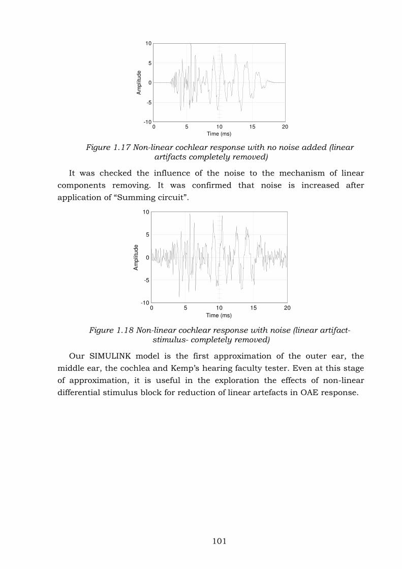
101
0 5 10 15 20-10
-5
0
5
10
Time (ms)A
mp
litu
de
Figure 1.17 Non-linear cochlear response with no noise added (linear artifacts completely removed)
It was checked the influence of the noise to the mechanism of linear
components removing. It was confirmed that noise is increased after
application of “Summing circuit”.
0 5 10 15 20-10
-5
0
5
10
Time (ms)
Am
plitu
de
Figure 1.18 Non-linear cochlear response with noise (linear artifact-stimulus- completely removed)
Our SIMULINK model is the first approximation of the outer ear, the
middle ear, the cochlea and Kemp’s hearing faculty tester. Even at this stage
of approximation, it is useful in the exploration the effects of non-linear
differential stimulus block for reduction of linear artefacts in OAE response.