Biostatistics Made Easy: A Guide for Air Force Public Health

Professionals

Contents

1. Data display and summary

2. Mean and standard deviation

3. Populations and samples

4. Statements of probability and confidence intervals

5. Differences between means: type I and type II errors and power

6. Differences between percentages and paired alternatives

7. The t-tests

8. The chi-squared tests

9. Exact probability test

10. Rank score tests

11. Correlation and regression

12. Survival analysis

13. Study design and choosing a statistical test

Appendix A - Probabilities related to multiples of standard deviations for a Normal distribution

Appendix B - Distribution of t (two tailed)

Appendix C - Distribution of µ

Appendix D - Wilcoxon test on paired samples: 5% and 1% levels of P

Appendix E - Mann-Whitney test on unpaired samples: 5% and 1% levels of P

Appendix F - Random Numbers

Glossary of Statistical Terms

Adapted and Modified from: T.D.V. Swinscow, Statistics at Square One, 9th Edition, Revised by M.J. Campbell, University of Southampton, UK

Chapter 1. Data Display and Summary

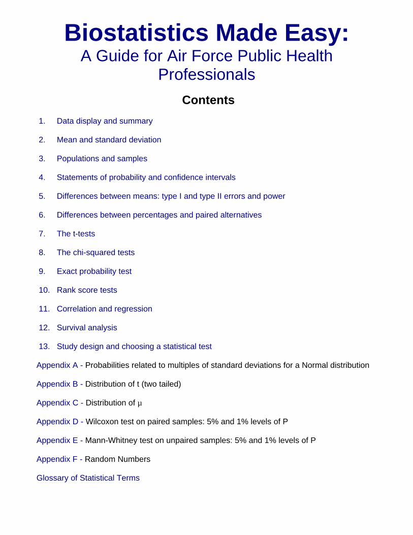
Types of data The first step, before any calculations or plotting of data, is to decide what type of data one is dealing with. There are a number of typologies, but one that has proven useful is given in Table 1.1. The basic distinction is between quantitative variables (for which one asks "how much?") and categorical variables (for which one asks "what type?").

Quantitative variables can be continuous or discrete. Continuous variables, such as height, can in theory take any value within a given range. Examples of discrete variables are: number of children in a family, number of attacks of asthma per week.

Categorical variables are either nominal (unordered) or ordinal (ordered). Examples of nominal variables are male/female, alive/dead, blood group O, A, B, AB. For nominal variables with more than two categories the order does not matter. For example, one cannot say that people in blood group B lie between those in A and those in AB. Sometimes, however, people can provide ordered responses, such as grade of breast cancer, or they can "agree", "neither agree nor disagree", or "disagree" with some statement. In this case the order does matter and it is usually important to account for it.

Table 1.1 Examples of types of data

Quantitative

Continuous Discrete

Blood pressure, height, weight, age

Number of children Number of attacks of asthma per week

Categorical

Ordinal (Ordered categories)

Nominal (Unordered categories)

Grade of breast cancer Better, same, worse Disagree, neutral, agree

Sex (male/female) Alive or dead Blood group O, A, B, AB

Variables shown at the left of Table 1.1 can be converted to ones further to the right by using "cut off points". For example, blood pressure can be turned into a nominal variable by defining "hypertension" as a diastolic blood pressure greater than 90 mmHg, and "normotension" as blood pressure less than or equal to 90 mmHg. Height (continuous) can be converted into "short", "average" or "tall" (ordinal).

In general it is easier to summarize categorical variables, and so quantitative variables are often converted to categorical ones for descriptive purposes. To make a clinical decision on someone, one does not need to know the exact serum potassium level (continuous) but whether it is within the normal range (nominal). It may be easier to think of the proportion of the population who are hypertensive than the distribution of blood pressure. However, categorizing a continuous variable reduces the amount of information available and statistical tests will in general be more sensitive - that is they will have more power (see Chapter 5 for a definition of power) for a continuous variable than the corresponding nominal one, although more assumptions may have to be made about the data. Categorizing data is therefore useful for summarizing results, but not for statistical analysis. It is often not appreciated that the choice of appropriate cut off points can be difficult, and different choices can lead to different conclusions about a set of data.

These definitions of types of data are not unique, nor are they mutually exclusive, and are given as an aid to help an investigator decide how to display and analyze data. One should not debate long over the typology of a particular variable!

Stem and leaf plots Before any statistical calculation, even the simplest, is performed the data should be tabulated or plotted. If they are quantitative and relatively few, say up to about 30, they are conveniently written down in order of size.

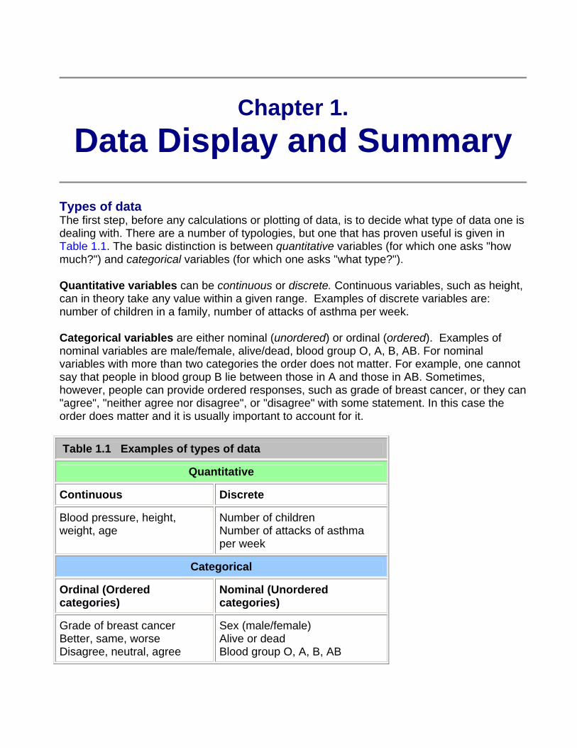
For example, a pediatric registrar in a district general hospital is investigating the amount of lead in the urine of children from a nearby housing estate. In a particular street there are 15 children whose ages range from 1 year to under 16, and in a preliminary study the registrar has found the following amounts of urinary lead ( ), given in Table 1.2 what is called an array:

Table 1.2 Urinary concentration of lead in 15 children from housing area X ( )

0.6, 2.6, 0.1, 1.1, 0.4, 2.0, 0.8, 1.3, 1.2, 1.5, 3.2, 1.7, 1.9, 1.9, 2.2

A simple way to order, and also to display, the data is to use a stem and leaf plot. To do this we need to abbreviate the observations to two significant digits. In the case of the urinary concentration data, the digit to the left of the decimal point is the "stem" and the digit to the right the "leaf".

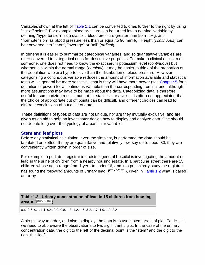
We first write the stems in order down the page. We then work along the data set, writing the leaves down "as they come". Thus, for the first data point, we write a 6 opposite the 0 stem. These are as given in Figure 1.1.

Figure 1.1 Stem and leaf "as they come"

Stem Leaf

0 6 1 4 8

1 1 3 2 5 7 9 9

2 6 0 2

3 2

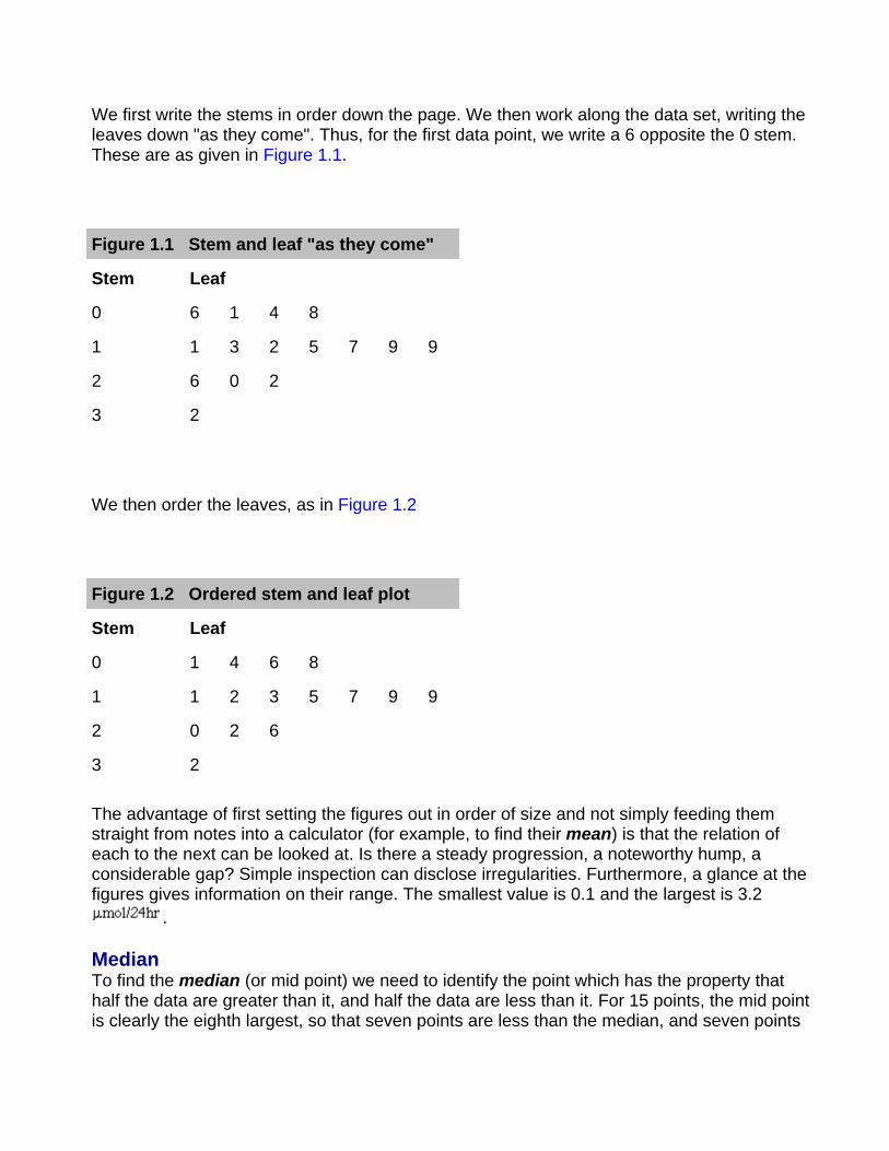
We then order the leaves, as in Figure 1.2

Figure 1.2 Ordered stem and leaf plot

Stem Leaf

0 1 4 6 8

1 1 2 3 5 7 9 9

2 0 2 6

3 2

The advantage of first setting the figures out in order of size and not simply feeding them straight from notes into a calculator (for example, to find their mean) is that the relation of each to the next can be looked at. Is there a steady progression, a noteworthy hump, a considerable gap? Simple inspection can disclose irregularities. Furthermore, a glance at the figures gives information on their range. The smallest value is 0.1 and the largest is 3.2

.

Median To find the median (or mid point) we need to identify the point which has the property that half the data are greater than it, and half the data are less than it. For 15 points, the mid point is clearly the eighth largest, so that seven points are less than the median, and seven points

are greater than it. This is easily obtained from Figure 1.2 by counting the eighth leaf, which is 1.5 .

To find the median for an even number of points, the procedure is as follows. Suppose the pediatric registrar obtained a further set of 16 urinary lead concentrations from children living in the countryside in the same county as the hospital? (Table 1.3)

Table 1.3 Urinary concentration of lead in 16 rural children ( )

0.2, 0.3, 0.6, 0.7, 0.8, 1.5, 1.7, 1.8, 1.9, 1.9, 2.0, 2.0, 2.1, 2.8, 3.1, 3.4

To obtain the median we average the eighth and ninth points (1.8 and 1.9) to get 1.85 . In general, if n is even, we average the n/2nd largest and the n/2 + 1st largest observations.

The main advantage of using the median as a measure of location is that it is "robust" to outliers. For example, if we had accidentally written 34 rather than 3.4 in Table 1.2 , the median would still have been 1.85. One disadvantage is that it is tedious to order a large number of observations by hand (there is usually no "median" button on a calculator).

Measures of variation It is informative to have some measure of the variation of observations about the median. The range is very susceptible to what are known as outliers, points well outside the main body of the data. For example, if we had made the mistake of writing 34 instead 3.4 in Table 1.2, then the range would be written as 0.1 to 34 which is clearly misleading.

A more robust approach is to divide the distribution of the data into four, and find the points below which are 25%, 50% and 75% of the distribution. These are known as quartiles, and the median is the second quartile. The variation of the data can be summarized in the interquartile range, the distance between the first and third quartile. With small data sets and if the sample size is not divisible by four, it may not be possible to divide the data set into exact quarters, and there are a variety of proposed methods to estimate the quartiles. A simple, consistent method is to find the points midway between each end of the range and the median. Thus, from Figure 1.2, there are eight points between and including the smallest, 0.1, and the median, 1.5. Thus the mid point lies between 0.8 and 1.1, or 0.95. This is the first quartile. Similarly the third quartile is mid-way between 1.9 and 2.0, or 1.95. Thus, the interquartile range is 0.95 to 1.95 .

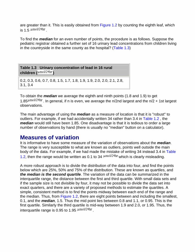
Data display The simplest way to show data is a dot plot. Figure 1.3 shows the data from Tables 1.2 and 1.3 and together with the median for each set.

Figure 1.3 Dot plot of urinary lead concentrations for urban and rural children.

Sometimes the points in separate plots may be linked in some way, for example the data in Table 1.2 and Table 1.3 may result from a matched case control study (see Chapter 13 for a description of this type of study) in which individuals from the countryside were matched by age and sex with individuals from the town. If possible the links should be maintained in the display, for example by joining matching individuals in Figure 1.3. This can lead to a more sensitive way of examining the data.

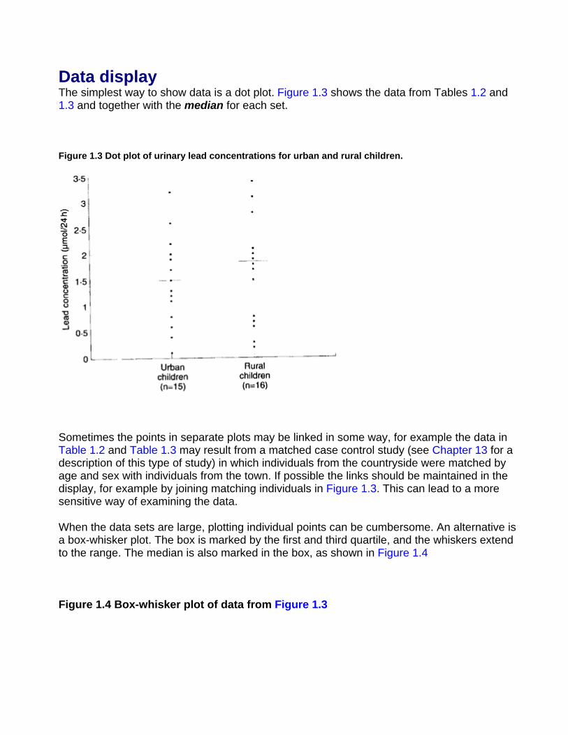
When the data sets are large, plotting individual points can be cumbersome. An alternative is a box-whisker plot. The box is marked by the first and third quartile, and the whiskers extend to the range. The median is also marked in the box, as shown in Figure 1.4

Figure 1.4 Box-whisker plot of data from Figure 1.3

It is easy to include more information in a box-whisker plot. One method, which is implemented in some computer programs, is to extend the whiskers only to points that are 1.5 times the interquartile range below the first quartile or above the third quartile, and to show remaining points as dots, so that the number of outlying points is shown.

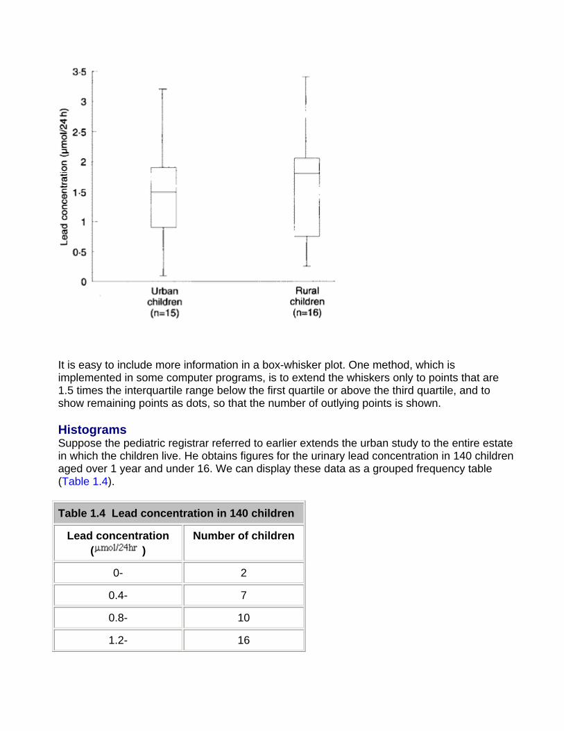
Histograms Suppose the pediatric registrar referred to earlier extends the urban study to the entire estate in which the children live. He obtains figures for the urinary lead concentration in 140 children aged over 1 year and under 16. We can display these data as a grouped frequency table (Table 1.4).

Table 1.4 Lead concentration in 140 children

Lead concentration ( )

Number of children

0- 2

0.4- 7

0.8- 10

1.2- 16

1.6- 23

2.0- 28

2.4 19

2.8- 16

3.2- 11

3.6- 7

2.4 19

2.8- 16

3.2- 11

3.6- 7

4.0- 1

4.4-

Total 140

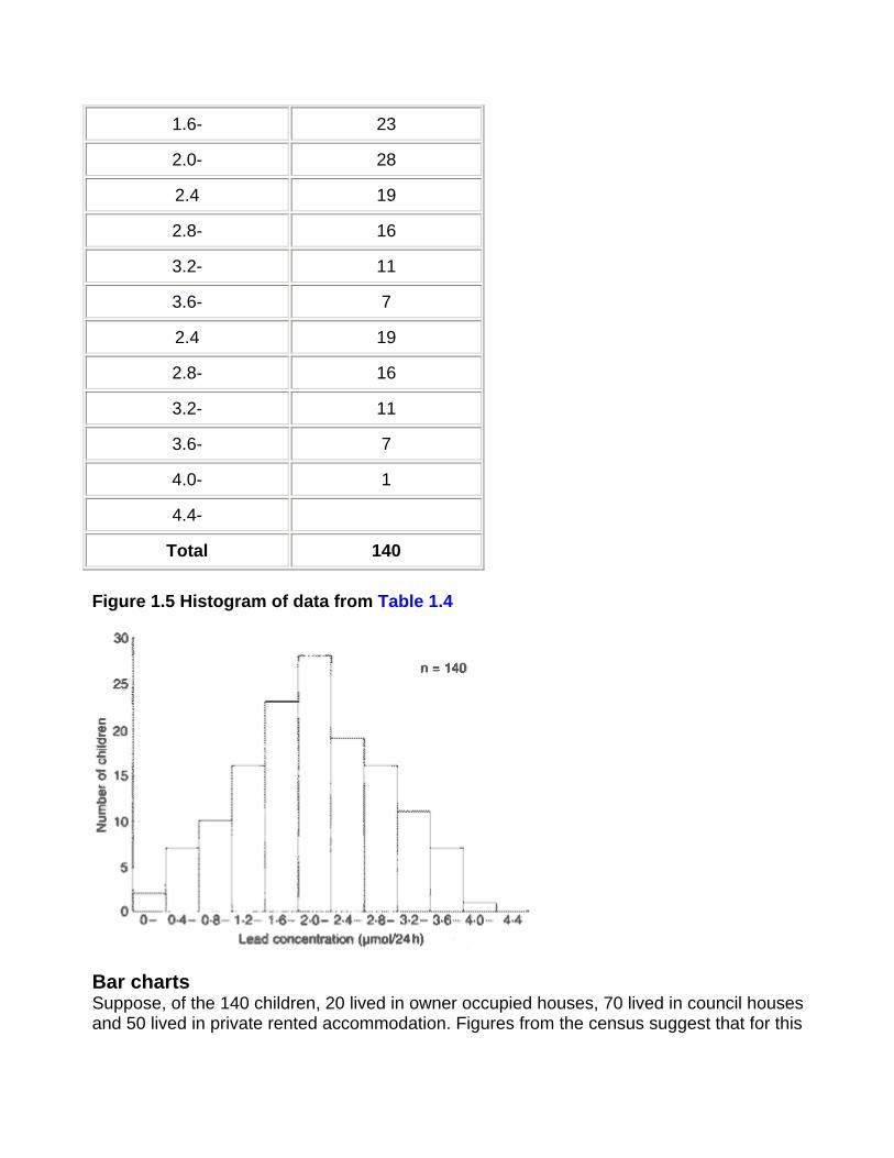
Figure 1.5 Histogram of data from Table 1.4

Bar charts Suppose, of the 140 children, 20 lived in owner occupied houses, 70 lived in council houses and 50 lived in private rented accommodation. Figures from the census suggest that for this

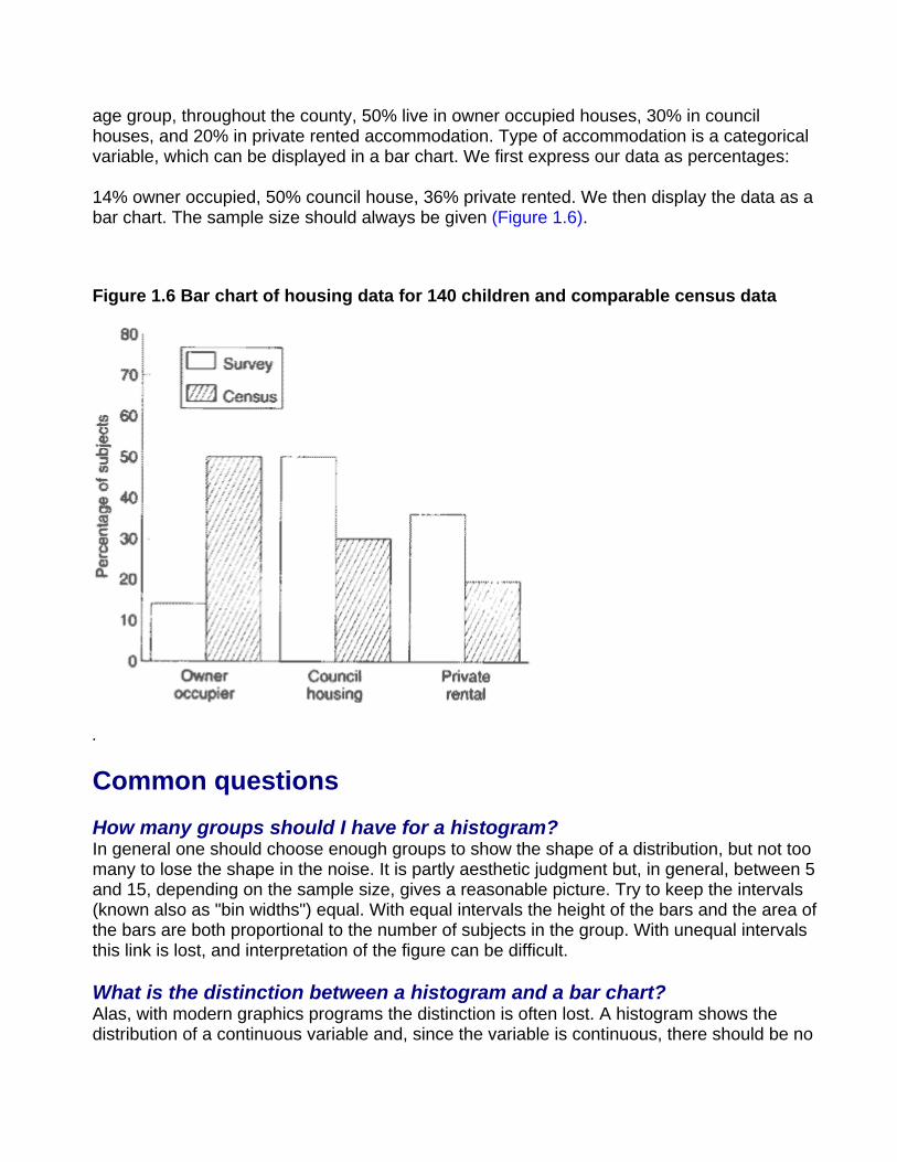
age group, throughout the county, 50% live in owner occupied houses, 30% in council houses, and 20% in private rented accommodation. Type of accommodation is a categorical variable, which can be displayed in a bar chart. We first express our data as percentages:

14% owner occupied, 50% council house, 36% private rented. We then display the data as a bar chart. The sample size should always be given (Figure 1.6).

Figure 1.6 Bar chart of housing data for 140 children and comparable census data

.

Common questions

How many groups should I have for a histogram? In general one should choose enough groups to show the shape of a distribution, but not too many to lose the shape in the noise. It is partly aesthetic judgment but, in general, between 5 and 15, depending on the sample size, gives a reasonable picture. Try to keep the intervals (known also as "bin widths") equal. With equal intervals the height of the bars and the area of the bars are both proportional to the number of subjects in the group. With unequal intervals this link is lost, and interpretation of the figure can be difficult.

What is the distinction between a histogram and a bar chart? Alas, with modern graphics programs the distinction is often lost. A histogram shows the distribution of a continuous variable and, since the variable is continuous, there should be no

gaps between the bars. A bar chart shows the distribution of a discrete variable or a categorical one, and so will have spaces between the bars. It is a mistake to use a bar chart to display a summary statistic such as a mean, particularly when it is accompanied by some measure of variation to produce a "dynamite plunger plot"(1). It is better to use a box-whisker plot.

What is the best way to display data? The general principle should be, as far as possible, to show the original data and to try not to obscure the design of a study in the display. Within the constraints of legibility show as much information as possible. If data points are matched or from the same patients link them with lines. (2) When displaying the relationship between two quantitative variables, use a scatter plot (Chapter 11) in preference to categorizing one or both of the variables.

References 1. Campbell M J. How to present numerical results. In: How to do it: 2. London: BMJ Publishing, 1995:77-83. 2. Matthews J N S, Altman D G, Campbell M J, Royston J P. Analysis of serial measurements in medical research. BMJ1990; 300:230-5.

Exercises

Exercise 1.1 From the 140 children whose urinary concentration of lead were investigated 40 were chosen who were aged at least 1 year but under 5 years. The following concentrations of copper (in ) were found.

0.70, 0.45, 0.72, 0.30, 1.16, 0.69, 0.83, 0.74, 1.24, 0.77,

0.65, 0.76, 0.42, 0.94, 0.36, 0.98, 0.64, 0.90, 0.63, 0.55,

0.78, 0.10, 0.52, 0.42, 0.58, 0.62, 1.12, 0.86, 0.74, 1.04,

0.65, 0.66, 0.81, 0.48, 0.85, 0.75, 0.73, 0.50, 0.34, 0.88

Find the median, range, and quartiles.

Chapter 2. Mean and Standard

Deviation

The median is known as a measure of location; that is, it tells us where the data are. As stated in, we do not need to know all the exact values to calculate the median; if we made the smallest value even smaller or the largest value even larger, it would not change the value of the median. Thus the median does not use all the information in the data and so it can be shown to be less efficient than the mean or average, which does use all values of the data. To calculate the mean we add up the observed values and divide by the number of them. The total of the values obtained in Table 1.1 was 22.5 , which was divided by their number, 15, to give a mean of 1.5 . This familiar process is conveniently expressed by the following symbols:

(pronounced "x bar") signifies the mean; x is each of the values of urinary lead; n is the number of these values; and , the Greek capital sigma (our "S") denotes "sum of". A major disadvantage of the mean is that it is sensitive to outlying points. For example, replacing 2.2 by 22 in Table 1.1 increases the mean to 2.82 , whereas the median will be unchanged.

As well as measures of location we need measures of how variable the data are. We met two of these measures, the range and interquartile range, in Chapter 1.

The range is an important measurement, for figures at the top and bottom of it denote the findings furthest removed from the generality. However, they do not give much indication of the spread of observations about the mean. This is where the standard deviation (SD) comes in.

The theoretical basis of the standard deviation is complex and need not trouble the ordinary user. We will discuss Sampling and Populations in Chapter 3. A practical point to note here is that, when the population from which the data arise have a distribution that is approximately "Normal" (or Gaussian), then the standard deviation provides a useful basis for interpreting the data in terms of probability.

The Normal distribution is represented by a family of curves defined uniquely by two parameters, which are the mean and the standard deviation of the population. The curves are always symmetrically bell shaped, but the extent to which the bell is compressed or flattened out depends on the standard deviation of the population. However, the mere fact that a curve is bell shaped does not mean that it represents a Normal distribution, because other distributions may have a similar sort of shape.

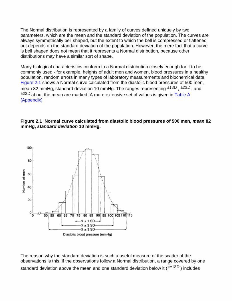
Many biological characteristics conform to a Normal distribution closely enough for it to be commonly used - for example, heights of adult men and women, blood pressures in a healthy population, random errors in many types of laboratory measurements and biochemical data. Figure 2.1 shows a Normal curve calculated from the diastolic blood pressures of 500 men, mean 82 mmHg, standard deviation 10 mmHg. The ranges representing , , and

about the mean are marked. A more extensive set of values is given in Table A (Appendix)

Figure 2.1 Normal curve calculated from diastolic blood pressures of 500 men, mean 82 mmHg, standard deviation 10 mmHg.

The reason why the standard deviation is such a useful measure of the scatter of the observations is this: if the observations follow a Normal distribution, a range covered by one standard deviation above the mean and one standard deviation below it ( ) includes

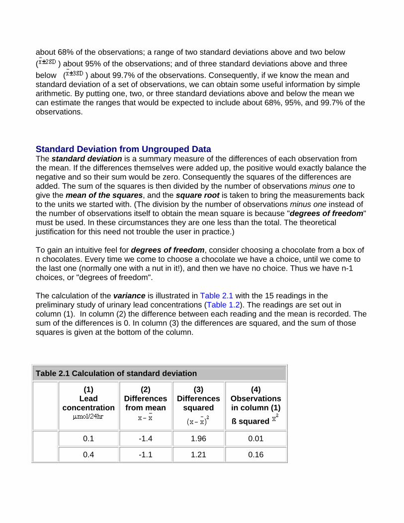
about 68% of the observations; a range of two standard deviations above and two below ( ) about 95% of the observations; and of three standard deviations above and three below ( ) about 99.7% of the observations. Consequently, if we know the mean and standard deviation of a set of observations, we can obtain some useful information by simple arithmetic. By putting one, two, or three standard deviations above and below the mean we can estimate the ranges that would be expected to include about 68%, 95%, and 99.7% of the observations.

Standard Deviation from Ungrouped Data The standard deviation is a summary measure of the differences of each observation from the mean. If the differences themselves were added up, the positive would exactly balance the negative and so their sum would be zero. Consequently the squares of the differences are added. The sum of the squares is then divided by the number of observations minus one to give the mean of the squares, and the square root is taken to bring the measurements back to the units we started with. (The division by the number of observations minus one instead of the number of observations itself to obtain the mean square is because "degrees of freedom" must be used. In these circumstances they are one less than the total. The theoretical justification for this need not trouble the user in practice.)

To gain an intuitive feel for degrees of freedom, consider choosing a chocolate from a box of n chocolates. Every time we come to choose a chocolate we have a choice, until we come to the last one (normally one with a nut in it!), and then we have no choice. Thus we have n-1 choices, or "degrees of freedom".

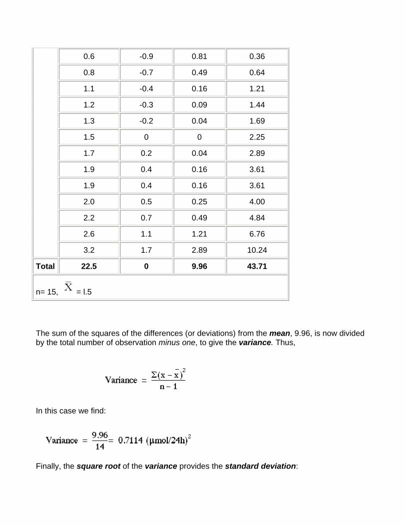
The calculation of the variance is illustrated in Table 2.1 with the 15 readings in the preliminary study of urinary lead concentrations (Table 1.2). The readings are set out in column (1). In column (2) the difference between each reading and the mean is recorded. The sum of the differences is 0. In column (3) the differences are squared, and the sum of those squares is given at the bottom of the column.

Table 2.1 Calculation of standard deviation

(1) Lead

concentration

(2) Differences from mean

(3) Differences

squared

(4) Observations in column (1) ß squared

0.1 -1.4 1.96 0.01

0.4 -1.1 1.21 0.16

0.6 -0.9 0.81 0.36

0.8 -0.7 0.49 0.64

1.1 -0.4 0.16 1.21

1.2 -0.3 0.09 1.44

1.3 -0.2 0.04 1.69

1.5 0 0 2.25

1.7 0.2 0.04 2.89

1.9 0.4 0.16 3.61

1.9 0.4 0.16 3.61

2.0 0.5 0.25 4.00

2.2 0.7 0.49 4.84

2.6 1.1 1.21 6.76

3.2 1.7 2.89 10.24

Total 22.5 0 9.96 43.71

n= 15, = l.5

The sum of the squares of the differences (or deviations) from the mean, 9.96, is now divided by the total number of observation minus one, to give the variance. Thus,

In this case we find:

Finally, the square root of the variance provides the standard deviation:

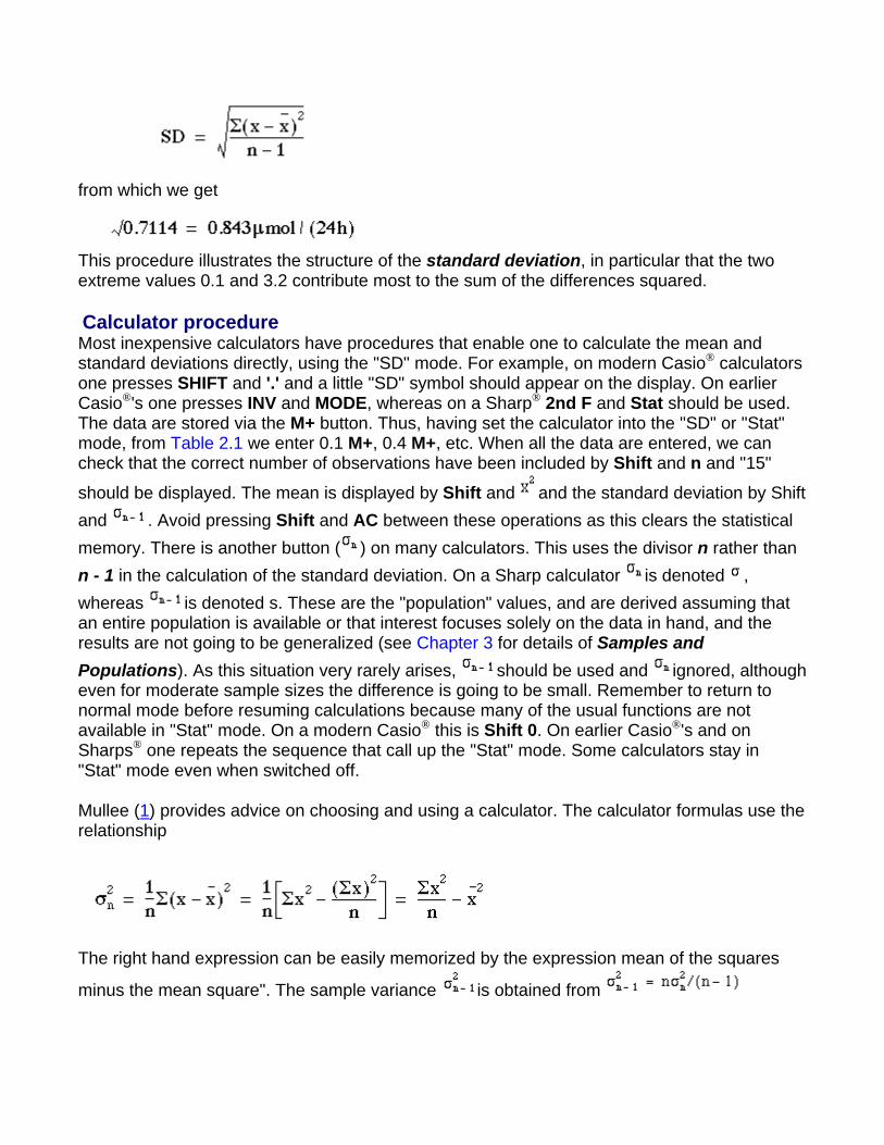
from which we get

This procedure illustrates the structure of the standard deviation, in particular that the two extreme values 0.1 and 3.2 contribute most to the sum of the differences squared.

Calculator procedure Most inexpensive calculators have procedures that enable one to calculate the mean and standard deviations directly, using the "SD" mode. For example, on modern Casio® calculators one presses SHIFT and '.' and a little "SD" symbol should appear on the display. On earlier Casio®'s one presses INV and MODE, whereas on a Sharp® 2nd F and Stat should be used. The data are stored via the M+ button. Thus, having set the calculator into the "SD" or "Stat" mode, from Table 2.1 we enter 0.1 M+, 0.4 M+, etc. When all the data are entered, we can check that the correct number of observations have been included by Shift and n and "15"

should be displayed. The mean is displayed by Shift and and the standard deviation by Shift and . Avoid pressing Shift and AC between these operations as this clears the statistical memory. There is another button ( ) on many calculators. This uses the divisor n rather than n - 1 in the calculation of the standard deviation. On a Sharp calculator is denoted , whereas is denoted s. These are the "population" values, and are derived assuming that an entire population is available or that interest focuses solely on the data in hand, and the results are not going to be generalized (see Chapter 3 for details of Samples and Populations). As this situation very rarely arises, should be used and ignored, although even for moderate sample sizes the difference is going to be small. Remember to return to normal mode before resuming calculations because many of the usual functions are not available in "Stat" mode. On a modern Casio® this is Shift 0. On earlier Casio®'s and on Sharps® one repeats the sequence that call up the "Stat" mode. Some calculators stay in "Stat" mode even when switched off.

Mullee (1) provides advice on choosing and using a calculator. The calculator formulas use the relationship

The right hand expression can be easily memorized by the expression mean of the squares

minus the mean square". The sample variance is obtained from

The above equation can be seen to be true in Table 2.1, where the sum of the square of the

observations, , is given as 43.7l. We thus obtain

the same value given for the total in column (3). Care should be taken because this formula involves subtracting two large numbers to get a small one, and can lead to incorrect results if the numbers are very large. For example, try finding the standard deviation of 100,001, 100,002, 100,003 on a calculator. The correct answer is 1, but many calculators will give 0 because of rounding error. The solution is to subtract a large number from each of the observations (say 100,000) and calculate the standard deviation on the remainders, namely 1, 2, and 3.

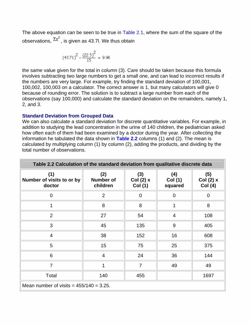
Standard Deviation from Grouped Data We can also calculate a standard deviation for discrete quantitative variables. For example, in addition to studying the lead concentration in the urine of 140 children, the pediatrician asked how often each of them had been examined by a doctor during the year. After collecting the information he tabulated the data shown in Table 2.2 columns (1) and (2). The mean is calculated by multiplying column (1) by column (2), adding the products, and dividing by the total number of observations.

Table 2.2 Calculation of the standard deviation from qualitative discrete data

(1) Number of visits to or by

doctor

(2) Number of children

(3) Col (2) x Col (1)

(4) Col (1)

squared

(5) Col (2) x Col (4)

0 2 0 0 0

1 8 8 1 8

2 27 54 4 108

3 45 135 9 405

4 38 152 16 608

5 15 75 25 375

6 4 24 36 144

7 1 7 49 49

Total 140 455 1697

Mean number of visits = 455/140 = 3.25.

As we did for continuous data, to calculate the standard deviation we square each of the observations in turn. In this case the observation is the number of visits, but because we have several children in each class, shown in column (2), each squared number (column (4)), must be multiplied by the number of children. The sum of squares is given at the foot of column (5), namely 1697. We then use the calculator formula to find the variance:

and

Note that although the number of visits is not Normally distributed, the distribution is reasonably symmetrical about the mean. The approximate 95% range is given by

This excludes two children with no visits and six children with six or more visits. Thus there are eight of 140 = 5.7% outside the theoretical 95% range.

Note that it is common for discrete quantitative variables to have what is known as skewed distributions, that is they are not symmetrical. One clue to lack of symmetry from derived statistics is when the mean and the median differ considerably. Another is when the standard deviation is of the same order of magnitude as the mean, but the observations must be non-negative. Sometimes a transformation will convert a skewed distribution into a symmetrical one. When the data are counts, such as number of visits to a doctor, often the square root transformation will help, and if there are no zero or negative values a logarithmic transformation will render the distribution more symmetrical.

Data Transformation An anesthetist measures the pain of a procedure using a 100mm visual analogue scale on seven patients. The results are given in Table 2.3, together with the loge transformation (the ln button on a calculator).

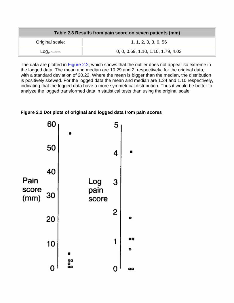
Table 2.3 Results from pain score on seven patients (mm)

Original scale: 1, 1, 2, 3, 3, 6, 56

Loge scale: 0, 0, 0.69, 1.10, 1.10, 1.79, 4.03

The data are plotted in Figure 2.2, which shows that the outlier does not appear so extreme in the logged data. The mean and median are 10.29 and 2, respectively, for the original data, with a standard deviation of 20.22. Where the mean is bigger than the median, the distribution is positively skewed. For the logged data the mean and median are 1.24 and 1.10 respectively, indicating that the logged data have a more symmetrical distribution. Thus it would be better to analyze the logged transformed data in statistical tests than using the original scale.

Figure 2.2 Dot plots of original and logged data from pain scores

.

In reporting these results, the median of the raw data would be given, but it should be explained that the statistical test was carried out on the transformed data. Note that the median of the logged data is the same as the log of the median of the raw data - however, this is not true for the mean. The mean of the logged data is not necessarily equal to the log of the mean

of the raw data. The antilog (exp or on a calculator) of the mean of the logged data is known as the geometric mean, and is often a better summary statistic than the mean for data from positively skewed distributions. For these data the geometric mean in 3.45 mm.

Between (inter-)subjects and Within (intra-)subjects Standard Deviation If repeated measurements are made of, say, blood pressure on an individual, these measurements are likely to vary. This is within subject, or intra-subject, variability and we can calculate a standard deviation of these observations. If the observations are close together in time, this standard deviation is often described as the measurement error. Measurements made on different subjects vary according to between subject, or inter-subject, variability. If many observations were made on each individual, and the average taken, then we can assume that the intra-subject variability has been averaged out and the variation in the average values is due solely to the inter-subject variability. Single observations on individuals clearly contain a mixture of inter-subject and intra-subject variation. The coefficient of variation (CV%) is the intra-subject standard deviation divided by the mean, expressed as a percentage. It is often quoted as a measure of repeatability for biochemical assays, when an assay is carried out on several occasions on the same sample. It has the advantage of being independent of the units of measurement, but also numerous theoretical disadvantages. It is usually nonsensical to use the coefficient of variation as a measure of between subject variability.

Common questions

When should I use the mean and when should I use the median to describe my data? It is a commonly held misapprehension that for Normally distributed data one uses the mean, and for non-Normally distributed data one uses the median. Unfortunately, this is not so: if the data are Normally distributed the mean and the median will be close; if the data are not Normally distributed then both the mean and the median may give useful information. Consider a variable that takes the value 1 for males and 0 for females. This is clearly not Normally distributed. However, the mean gives the proportion of males in the group, whereas the median merely tells us which group contained more than 50% of the people. Similarly, the mean from ordered categorical variables can be more useful than the median, if the ordered categories can be given meaningful scores. For example, a lecture might be rated as 1 (poor) to 5 (excellent). The usual statistic for summarizing the result would be the mean. In the situation where there is a small group at one extreme of a distribution (for example, annual income) then the median will be more "representative" of the distribution.

My data must have values greater than zero and yet the mean and standard deviation are about the same size. How does this happen? If data have a very skewed distribution, then the standard deviation will be grossly inflated, and is not a good measure of variability to use. As we have shown, occasionally a transformation of the data, such as a log transform, will render the distribution more symmetrical. Alternatively, quote the interquartile range.

References 1. Mullee M A. How to choose and use a calculator. In: How to do it 2.BMJ Publishing Group, 1995:58-62.

Exercises

Exercise 2.1 In the campaign against smallpox a doctor inquired into the number of times 150 people aged 16 and over in an Ethiopian village had been vaccinated. He obtained the following figures: never, 12 people; once, 24; twice, 42; three times, 38; four times, 30; five times, 4. What is the mean number of times those people had been vaccinated and what is the standard deviation?

Exercise 2.2 Obtain the mean and standard deviation of the data in and an approximate 95% range.

Exercise 2.3 Which points are excluded from the range mean - 2SD to mean + 2SD? What proportion of the data is excluded?

Chapter 3. Populations and Samples

Populations In statistics the term "population" has a slightly different meaning from the one given to it in ordinary speech. It need not refer only to people or to animate creatures - the population of Britain, for instance or the dog population of London. Statisticians also speak of a population of objects, or events, or procedures, or observations, including such things as the quantity of lead in urine, visits to the doctor, or surgical operations. A population is thus an aggregate of creatures, things, cases and so on.

Although a statistician should clearly define the population he or she is dealing with, they may not be able to enumerate it exactly. For instance, in ordinary usage the population of England denotes the number of people within England's boundaries, perhaps as enumerated at a census. But a physician might embark on a study to try to answer the question "What is the average systolic blood pressure of Englishmen aged 40-59?" But who are the "Englishmen" referred to here? Not all Englishmen live in England, and the social and genetic background of those that do may vary. A surgeon may study the effects of two alternative operations for gastric ulcer. But how old are the patients? What sex are they? How severe is their disease? Where do they live? And so on. The reader needs precise information on such matters to draw valid inferences from the sample that was studied to the population being considered. Statistics such as averages and standard deviations, when taken from populations are referred to as population parameters. They are often denoted by Greek letters: the population mean is

denoted by (mu) and the standard deviation denoted by (lower case sigma).

Samples A population commonly contains too many individuals to study conveniently, so an investigation is often restricted to one or more samples drawn from it. A well chosen sample will contain most of the information about a particular population parameter but the relation between the sample and the population must be such as to allow true inferences to be made about a population from that sample.

Consequently, the first important attribute of a sample is that every individual in the population from which it is drawn must have a known non-zero chance of being included in it; a natural suggestion is that these chances should be equal. We would like the choices to be made independently; in other words, the choice of one subject will not affect the chance of other subjects being chosen. To ensure this we make the choice by means of a process in which

chance alone operates, such as spinning a coin or, more usually, the use of a table of random numbers. A limited table is given in the Table F (Appendix), and more extensive ones have been published.(1-4) A sample so chosen is called a random sample. The word "random" does not describe the sample as such but the way in which it is selected.

To draw a satisfactory sample sometimes presents greater problems than to analyze statistically the observations made on it. A full discussion of the topic is beyond the scope of this book, but guidance is readily available(1)(2). In this book only an introduction is offered.

Before drawing a sample the investigator should define the population from which it is to come. Sometimes he or she can completely enumerate its members before beginning analysis - for example, all the livers studied at necropsy over the previous year, all the patients aged 20-44 admitted to hospital with perforated peptic ulcer in the previous 20 months. In retrospective studies of this kind numbers can be allotted serially from any point in the table to each patient or specimen. Suppose we have a population of size 150, and we wish to take a sample of size five. contains a set of computer generated random digits arranged in groups of five. Choose any row and column, say the last column of five digits. Read only the first three digits, and go down the column starting with the first row. Thus we have 265, 881, 722, etc. If a number appears between 001 and 150 then we include it in our sample. Thus, in order, in the sample will be subjects numbered 24, 59, 107, 73, and 65. If necessary we can carry on down the next column to the left until the full sample is chosen.

The use of random numbers in this way is generally preferable to taking every alternate patient or every fifth specimen, or acting on some other such regular plan. The regularity of the plan can occasionally coincide by chance with some unforeseen regularity in the presentation of the material for study - for example, by hospital appointments being made from patients from certain practices on certain days of the week, or specimens being prepared in batches in accordance with some schedule.

As susceptibility to disease generally varies in relation to age, sex, occupation, family history, exposure to risk, inoculation state, country lived in or visited, and many other genetic or environmental factors, it is advisable to examine samples when drawn to see whether they are, on average, comparable in these respects. The random process of selection is intended to make them so, but sometimes it can by chance lead to disparities. To guard against this possibility the sampling may be stratified. This means that a framework is laid down initially, and the patients or objects of the study in a random sample are then allotted to the compartments of the framework. For instance, the framework might have a primary division into males and females and then a secondary division of each of those categories into five age groups, the result being a framework with ten compartments. It is then important to bear in mind that the distributions of the categories on two samples made up on such a framework may be truly comparable, but they will not reflect the distribution of these categories in the population from which the sample is drawn unless the compartments in the framework have been designed with that in mind. For instance, equal numbers might be admitted to the male and female categories, but males and females are not equally numerous in the general population, and their relative proportions vary with age. This is known as stratified random sampling. For taking a sample from a long list a compromise between strict theory and

practicalities is known as a systematic random sample. In this case we choose subjects a fixed interval apart on the list, say every tenth subject, but we choose the starting point within the first interval at random.

Unbiasedness and Precision The terms unbiased and precision have acquired special meanings in statistics. When we say that a measurement is unbiased we mean that the average of a large set of unbiased measurements will be close to the true value. When we say it is precise we mean that it is repeatable. Repeated measurements will be close to one another, but not necessarily close to the true value. We would like a measurement that is both accurate and precise. Some authors equate unbiasedness with accuracy, but this is not universal and others use the term accuracy to mean a measurement that is both unbiased and precise. Strike(5) gives a good discussion of the problem.

An estimate of a parameter taken from a random sample is known to be unbiased. As the sample size increases, it gets more precise.

Randomization Another use of random number tables is to randomize the allocation of treatments to patients in a clinical trial. This ensures that there is no bias in treatment allocation and, in the long run, the subjects in each treatment group are comparable in both known and unknown prognostic factors. A common method is to use blocked randomization. This is to ensure that at regular intervals there are equal numbers in the two groups. Usual sizes for blocks are two, four, six, eight, and ten. Suppose we chose a block size of ten. A simple method using Table F (Appendix) is to choose the first five unique digits in any row. If we chose the first row, the first five unique digits are 3, 5, 6, 8, and 4. Thus we would allocate the third, fourth, fifth, sixth, and eighth subjects to one treatment and the first, second, seventh, ninth, and tenth to the other. If the block size was less than ten we would ignore digits bigger than the block size. To allocate further subjects to treatment, we carry on along the same row, choosing the next five unique digits for the first treatment. In randomized controlled trials it is advisable to change the block size from time to time to make it more difficult to guess what the next treatment is going to be.

It is important to realize that patients in a randomized trial are nota random sample from the population of people with the disease in question but rather a highly selected set of eligible and willing patients. However, randomization ensures that in the long run any differences in outcome in the two treatment groups are due solely to differences in treatment.

Variation between samples Even if we ensure that every member of a population has a known, and usually an equal, chance of being included in a sample, it does not follow that a series of samples drawn from

one population and fulfilling this criterion will be identical. They will show chance variations from one to another, and the variation may be slight or considerable. For example, a series of samples of the body temperature of healthy people would show very little variation from one to another, but the variation between samples of the systolic blood pressure would be considerable. Thus the variation between samples depends partly on the amount of variation in the population from which they are drawn.

Furthermore, it is a matter of common observation that a small sample is a much less certain guide to the population from which it was drawn than a large sample. In other words, the more members of a population that are included in a sample the more chance will that sample have of accurately representing the population, provided a random process is used to construct the sample. A consequence of this is that, if two or more samples are drawn from a population, the larger they are the more likely they are to resemble each other - again provided that the random technique is followed. Thus the variation between samples depends partly also on the size of the sample. Usually, however, we are not in a position to take a random sample; our sample is simply those subjects available for study. This is a "convenience" sample. For valid generalizations to be made we would like to assert that our sample is in some way representative of the population as a whole and for this reason the first stage in a report is to describe the sample, say by age, sex, and disease status, so that other readers can decide if it is representative of the type of patients they encounter.

Standard error of the mean If we draw a series of samples and calculate the mean of the observations in each, we have a series of means. These means generally conform to a Normal distribution, and they often do so even if the observations from which they were obtained do not (see Exercise 3.3). This can be proven mathematically and is known as the "Central Limit Theorem". The series of means, like the series of observations in each sample, has a standard deviation. The standard error of the mean of one sample is an estimate of the standard deviation that would be obtained from the means of a large number of samples drawn from that population.

As noted above, if random samples are drawn from a population their means will vary from one to another. The variation depends on the variation of the population and the size of the sample. We do not know the variation in the population so we use the variation in the sample as an estimate of it. This is expressed in the standard deviation. If we now divide the standard deviation by the square root of the number of observations in the sample we have an estimate of the standard error of the mean, . It is important to realize that we do not have to take repeated samples in order to estimate the standard error, there is sufficient information within a single sample. However, the conception is that if we were to take repeated random samples from the population, this is how we would expect the mean to vary, purely by chance.

A general practitioner in Yorkshire has a practice which includes part of a town with a large printing works and some of the adjacent sheep farming country. With her patients' informed consent she has been investigating whether the diastolic blood pressure of men aged 20-44 differs between the printers and the farm workers. For this purpose she has obtained a random

sample of 72 printers and 48 farm workers and calculated the mean and standard deviations, as shown in Table 3.1.

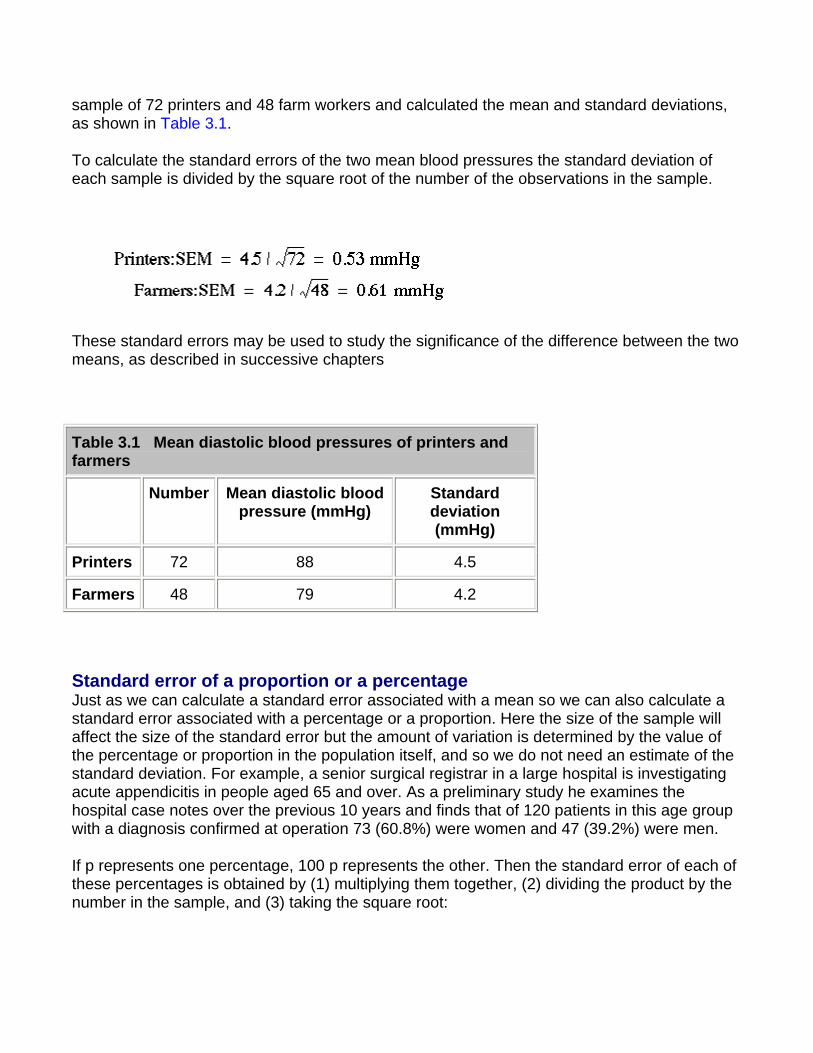
To calculate the standard errors of the two mean blood pressures the standard deviation of each sample is divided by the square root of the number of the observations in the sample.

These standard errors may be used to study the significance of the difference between the two means, as described in successive chapters

Table 3.1 Mean diastolic blood pressures of printers and farmers

Number Mean diastolic blood pressure (mmHg)

Standard deviation (mmHg)

Printers 72 88 4.5

Farmers 48 79 4.2

Standard error of a proportion or a percentage Just as we can calculate a standard error associated with a mean so we can also calculate a standard error associated with a percentage or a proportion. Here the size of the sample will affect the size of the standard error but the amount of variation is determined by the value of the percentage or proportion in the population itself, and so we do not need an estimate of the standard deviation. For example, a senior surgical registrar in a large hospital is investigating acute appendicitis in people aged 65 and over. As a preliminary study he examines the hospital case notes over the previous 10 years and finds that of 120 patients in this age group with a diagnosis confirmed at operation 73 (60.8%) were women and 47 (39.2%) were men.

If p represents one percentage, 100 p represents the other. Then the standard error of each of these percentages is obtained by (1) multiplying them together, (2) dividing the product by the number in the sample, and (3) taking the square root:

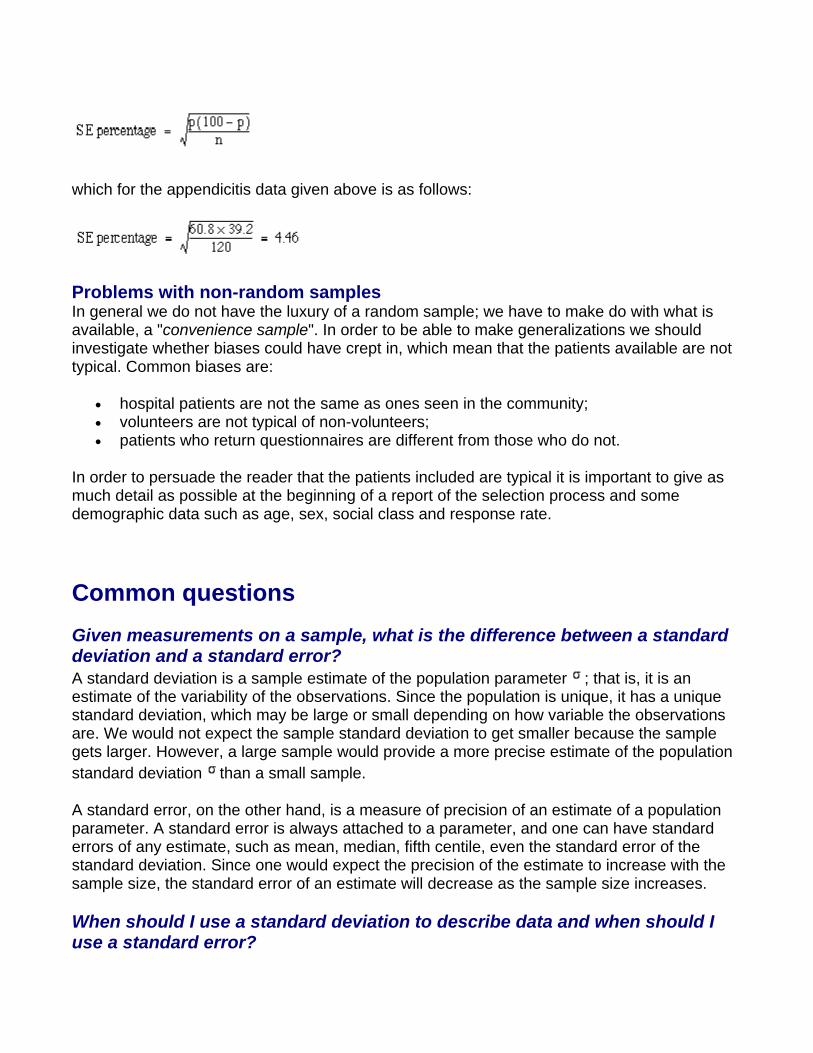
which for the appendicitis data given above is as follows:

Problems with non-random samples In general we do not have the luxury of a random sample; we have to make do with what is available, a "convenience sample". In order to be able to make generalizations we should investigate whether biases could have crept in, which mean that the patients available are not typical. Common biases are:

• hospital patients are not the same as ones seen in the community; • volunteers are not typical of non-volunteers; • patients who return questionnaires are different from those who do not.

In order to persuade the reader that the patients included are typical it is important to give as much detail as possible at the beginning of a report of the selection process and some demographic data such as age, sex, social class and response rate.

Common questions

Given measurements on a sample, what is the difference between a standard deviation and a standard error? A standard deviation is a sample estimate of the population parameter ; that is, it is an estimate of the variability of the observations. Since the population is unique, it has a unique standard deviation, which may be large or small depending on how variable the observations are. We would not expect the sample standard deviation to get smaller because the sample gets larger. However, a large sample would provide a more precise estimate of the population standard deviation than a small sample.

A standard error, on the other hand, is a measure of precision of an estimate of a population parameter. A standard error is always attached to a parameter, and one can have standard errors of any estimate, such as mean, median, fifth centile, even the standard error of the standard deviation. Since one would expect the precision of the estimate to increase with the sample size, the standard error of an estimate will decrease as the sample size increases.

When should I use a standard deviation to describe data and when should I use a standard error?

It is a common mistake to try and use the standard error to describe data. Usually it is done because the standard error is smaller, and so the study appears more precise. If the purpose is to describe the data (for example so that one can see if the patients are typical) and if the data are plausibly Normal, then one should use the standard deviation (mnemonic D for Description and D for Deviation). If the purpose is to describe the outcome of a study, for example to estimate the prevalence of a disease, or the mean height of a group, then one should use a standard error (or, better, a confidence interval; see Chapter 4) (mnemonic E for Estimate and E for Error).

References

1 Altman DG. Practical Statistics for Medical Research. London: Chapman & Hall, 1991 2. Armitage P, Berry G. Statistical Methods in Medical Research. Oxford: Blackwell Scientific Publications, 1994. 3. Campbell MJ, Machin D. Medical Statistics: A Commonsense Approach.2nd ed. Chichester: John Wiley, 1993. 4. Fisher RA, Yates F. Statistical Tables for Biological, Agricultural and Medical Research,6th ed. London: Longman, 1974. 5. Strike PW. Measurement and control. Statistical Methods in Laboratory Medicine. Oxford: Butterworth-Heinemann, 1991:255.

Exercises

Exercise 3.1 The mean urinary lead concentration in 140 children was 2.18 mol/24 h, with standard deviation 0.87. What is the standard error of the mean?

Exercise 3.2 In Table F (Appendix), what is the distribution of the digits, and what are the mean and standard deviation?

Exercise 3.3 For the first column of five digits in Table F take the mean value of the five digits and do this for all rows of five digits in the column. What would you expect a histogram of the means to look like? What would you expect the mean and standard deviation to be?

Chapter 4. Statements of Probability and Confidence Intervals

We have seen that when a set of observations have a Normal distribution multiples of the standard deviation mark certain limits on the scatter of the observations. For instance, 1.96 (or approximately 2) standard deviations above and 1.96 standard deviations below the mean ( ) mark the points within which 95% of the observations lie.

Reference Ranges We noted in Chapter 1 that 140 children had a mean urinary lead concentration of 2.18

, with standard deviation 0.87. The points that include 95% of the observations are 2.18 ± (1.96 × 0.87), giving a range of 0.48 to 3.89. One of the children had a urinary lead concentration of just over 4.0 . This observation is greater than 3.89 and so falls in the 5% beyond the 95% probability limits. We can say that the probability of each of such observations occurring is 5% or less. Another way of looking at this is to see that if one chose one child at random out of the 140, the chance that their urinary lead concentration exceeded 3.89 or was less than 0.48 is 5%. This probability is usually used expressed as a fraction of 1 rather than of 100, and written

Standard deviations thus set limits about which probability statements can be made. Some of these are set out in Table A (appendix). To use to estimate the probability of finding an observed value, say a urinary lead concentration of 4 , in sampling from the same population of observations as the 140 children provided, we proceed as follows. The distance of the new observation from the mean is 4.8 - 2.18 = 2.62. How many standard deviations does this represent? Dividing the difference by the standard deviation gives 2.62/0.87 = 3.01. This number is greater than 2.576 but less than 3.291 in , so the probability of finding a deviation as large or more extreme than this lies between 0.01 and 0.001, which maybe expressed as In fact Table A shows that the probability is very close to 0.0027. This probability is small, so the observation probably did not come from the same population as the 140 other children.

To take another example, the mean diastolic blood pressure of printers was found to be 88 mmHg and the standard deviation 4.5 mmHg. One of the printers had a diastolic blood pressure of 100 mmHg. The mean plus or minus 1.96 times its standard deviation gives the following two figures:

88 + (1.96 x 4.5) = 96.8 mmHg

88 - (1.96 x 4.5) = 79.2 mmHg.

We can say therefore that only 1 in 20 (or 5%) of printers in the population from which the sample is drawn would be expected to have a diastolic blood pressure below 79 or above about 97 mmHg. These are the 95% limits. The 99.73% limits lie three standard deviations below and three above the mean. The blood pressure of 100 mmHg noted in one printer thus lies beyond the 95% limit of 97 but within the 99.73% limit of 101.5 (= 88 + (3 x 4.5)).

The 95% limits are often referred to as a "reference range". For many biological variables, they define what is regarded as the normal (meaning standard or typical) range. Anything outside the range is regarded as abnormal. Given a sample of disease free subjects, an alternative method of defining a normal range would be simply to define points that exclude 2.5% of subjects at the top end and 2.5% of subjects at the lower end. This would give an empirical normal range. Thus in the 140 children we might choose to exclude the three highest and three lowest values. However, it is much more efficient to use the mean 2 SD, unless the data set is quite large (say ).

Confidence Intervals (CI) The means and their standard errors can be treated in a similar fashion. If a series of samples are drawn and the mean of each calculated, 95% of the means would be expected to fall within the range of two standard errors above and two below the mean of these means. This common mean would be expected to lie very close to the mean of the population. So the standard error of a mean provides a statement of probability about the difference between the mean of the population and the mean of the sample.

In our sample of 72 printers, the standard error of the mean was 0.53 mmHg. The sample mean plus or minus 196 times its standard error gives the following two figures:

88 + (1.96 x 0.53) = 89.04 mmHg

88 - (1.96 x 0.53) = 86.96 mmHg.

This is called the 95% confidence interval, and we can say that there is only a 5% chance that the range 86.96 to 89.04 mmHg excludes the mean of the population. If we take the mean plus or minus three times its standard error, the range would be 86.41 to 89.59. This is the 99.73% confidence interval, and the chance of this range excluding the population mean is 1 in 370. Confidence intervals provide the key to a useful device for arguing from a sample back to the population from which it came.

The standard error for the percentage of male patients with appendicitis, described in Chapter 3, was 4.46. This is also the standard error of the percentage of female patients with appendicitis, since the formula remains the same if p is replaced by 100 - p. With this standard error we can get 95% confidence intervals on the two percentages:

60.8 (1.96 x 4.46) = 52.1 and 69.5

39.2 (1.96 x 4.46) = 30.5 and 47.9.

These confidence intervals exclude 50%. Can we conclude that males are more likely to get appendicitis? This is the subject of the rest of the book, namely inference .

With small samples - say under 30 observations - larger multiples of the standard error are needed to set confidence limits. This subject is discussed under the t distribution (Chapter 7).

There is much confusion over the interpretation of the probability attached to confidence intervals. To understand it we have to resort to the concept of repeated sampling. Imagine taking repeated samples of the same size from the same population. For each sample calculate a 95% confidence interval. Since the samples are different, so are the confidence intervals. We know that 95% of these intervals will include the population parameter. However, without any additional information we cannot say which ones! Thus with only one sample, and no other information about the population parameter, we can say there is a 95% chance of including the parameter in our interval. Note that this does not mean that we would expect with 95% probability that the mean from another sample is in this interval. In this case we are considering differences between two sample means, which is the subject of the next chapter.

Common questions

What is the difference between a reference range and a confidence interval? There is precisely the same relationship between a reference range and a confidence interval as between the standard deviation and the standard error. The reference range refers to individuals and the confidence intervals to estimates . It is important to realize that samples are not unique. Different investigators taking samples from the same population will obtain different estimates, and have different 95% confidence intervals. However, we know that for 95 of every 100 investigators the confidence interval will include the population mean interval.

When should one quote a confidence interval? There is now a great emphasis on confidence intervals in the literature, and some authors attach them to every estimate they make. In general, unless the main purpose of a study is to actually estimate a mean or a percentage, confidence intervals are best restricted to the main outcome of a study, which is usually a contrast (that is, a difference) between means or percentages. This is the topic for the next two chapters.

Exercises Exercise 4.1 A count of malaria parasites in 100 fields with a 2mm oil immersion lens gave a mean of 35 parasites per field, standard deviation 11.6 (note that, although the counts are quantitative discrete, the counts can be assumed to follow a Normal distribution because the average is large). On counting one more field the pathologist found 52 parasites. Does this number lie outside the 95% reference range? What is the reference range?

Exercise 4.2 What is the 95% confidence interval for the mean of the population from which this sample count of parasites was drawn?

Chapter 5. Differences between Means: Type I and Type II Errors and

Power

We saw in Chapter 3 that the mean of a sample has a standard error, and a mean that departs by more than twice its standard error from the population mean would be expected by chance only in about 5% of samples. Likewise, the difference between the means of two samples has a standard error. We do not usually know the population mean, so we may suppose that the mean of one of our samples estimates it. The sample mean may happen to be identical with the population mean but it more probably lies somewhere above or below the population mean, and there is a 95% chance that it is within 1.96 standard errors of it.

Consider now the mean of the second sample. If the sample comes from the same population its mean will also have a 95% chance of lying within 196 standard errors of the population mean but if we do not know the population mean we have only the means of our samples to guide us. Therefore, if we want to know whether they are likely to have come from the same population, we ask whether they lie within a certain range, represented by their standard errors, of each other.

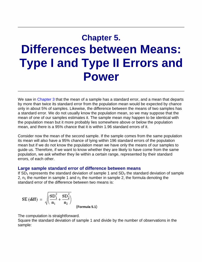
Large sample standard error of difference between means If SD1 represents the standard deviation of sample 1 and SD2 the standard deviation of sample 2, n1 the number in sample 1 and n2 the number in sample 2, the formula denoting the standard error of the difference between two means is:

(Formula 5.1)

The computation is straightforward. Square the standard deviation of sample 1 and divide by the number of observations in the sample:

(1)

Square the standard deviation of sample 2 and divide by the number of observations in the sample:

(2)

Add (1) and (2).

Take the square root, to give equation 5.1. This is the standard error of the difference between the two means.

Large sample confidence interval for the difference in two means From the data in the general practitioner wants to compare the mean of the printers' blood pressures with the mean of the farmers' blood pressures. The figures are set out first as in table 5.1 (which repeats table 3.1 ).

Table 5.1 Mean diastolic blood pressures of printers and farmers

Number Mean diastolic blood pressure (mmHg)

Standard deviation (mmHg)

Printers 72 88 4.5 Farmers 48 79 4.2

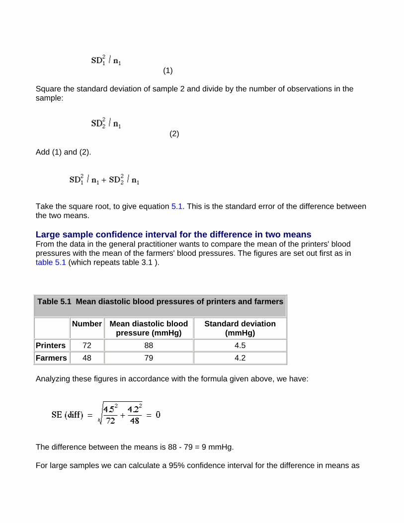
Analyzing these figures in accordance with the formula given above, we have:

The difference between the means is 88 - 79 = 9 mmHg.

For large samples we can calculate a 95% confidence interval for the difference in means as

9 - 1.96 x 0.81 to 9 + 1.96 x 0.81 which is 7.41 to 10.59 mmHg.

For a small sample we need to modify this procedure, as described in Chapter 7.

Null Hypothesis and Type I Error In comparing the mean blood pressures of the printers and the farmers we are testing the hypothesis that the two samples came from the same population of blood pressures. The hypothesis that there is no difference between the population from which the printers' blood pressures were drawn and the population from which the farmers' blood pressures were drawn is called the null hypothesis.

But what do we mean by "no difference"? Chance alone will almost certainly ensure that there is some difference between the sample means, for they are most unlikely to be identical. Consequently we set limits within which we shall regard the samples as not having any significant difference. If we set the limits at twice the standard error of the difference, and regard a mean outside this range as coming from another population, we shall on average be wrong about one time in 20 if the null hypothesis is in fact true. If we do obtain a mean difference bigger than two standard errors we are faced with two choices: either an unusual event has happened, or the null hypothesis is incorrect. Imagine tossing a coin five times and getting the same face each time. This has nearly the same probability (6.3%) as obtaining a mean difference bigger than two standard errors when the null hypothesis is true. Do we regard it as a lucky event or suspect a biased coin? If we are unwilling to believe in unlucky events, we reject the null hypothesis, in this case that the coin is a fair one.

To reject the null hypothesis when it is true is to make what is known as a type I error . The level at which a result is declared significant is known as the type I error rate, often denoted by

. We try to show that a null hypothesis is unlikely , not its converse (that it is likely), so a difference which is greater than the limits we have set, and which we therefore regard as "significant", makes the null hypothesis unlikely . However, a difference within the limits we have set, and which we therefore regard as "non-significant", does not make the hypothesis likely.

A range of not more than two standard errors is often taken as implying "no difference" but there is nothing to stop investigators choosing a range of three standard errors (or more) if they want to reduce the chances of a type I error.

Testing for Differences of Two Means To find out whether the difference in blood pressure of printers and farmers could have arisen by chance the general practitioner erects the null hypothesis that there is no significant difference between them. The question is, how many multiples of its standard error does the difference in means difference represent? Since the difference in means is 9 mmHg and its standard error is 0.81 mmHg, the answer is: 9/0.81 = 11.1. We usually denote the ratio of an

estimate to its standard error by "z", that is, z = 11.1. Reference to Table A (Appendix) shows that z is far beyond the figure of 3.291 standard deviations, representing a probability of 0.001 (or 1 in 1000). The probability of a difference of 11.1 standard errors or more occurring by chance is therefore exceedingly low, and correspondingly the null hypothesis that these two samples came from the same population of observations is exceedingly unlikely. The probability is known as the P value and may be written .

It is worth recapping this procedure, which is at the heart of statistical inference. Suppose that we have samples from two groups of subjects, and we wish to see if they could plausibly come from the same population. The first approach would be to calculate the difference between two statistics (such as the means of the two groups) and calculate the 95% confidence interval. If the two samples were from the same population we would expect the confidence interval to include zero 95% of the time, and so if the confidence interval excludes zero we suspect that they are from a different population. The other approach is to compute the probability of getting the observed value, or one that is more extreme , if the null hypothesis were correct. This is the P value. If this is less than a specified level (usually 5%) then the result is declared significant and the null hypothesis is rejected. These two approaches, the estimation and hypothesis testing approach, are complementary. Imagine if the 95% confidence interval just captured the value zero, what would be the P value? A moment's thought should convince one that it is 2.5%. This is known as a one sided P value , because it is the probability of getting the observed result or one bigger than it. However, the 95% confidence interval is two sided, because it excludes not only the 2.5% above the upper limit but also the 2.5% below the lower limit. To support the complementarity of the confidence interval approach and the null hypothesis testing approach, most authorities double the one sided P value to obtain a two sided P value (see below for the distinction between one sided and two sided tests).

Sometimes an investigator knows a mean from a very large number of observations and wants to compare the mean of her sample with it. We may not know the standard deviation of the large number of observations or the standard error of their mean but this need not hinder the comparison if we can assume that the standard error of the mean of the large number of observations is near zero or at least very small in relation to the standard error of the mean of the small sample.

This is because in equation 5.1 for calculating the standard error of the difference between the

two means, when n1is very large then becomes so small as to be negligible. The formula thus reduces to

which is the same as that for standard error of the sample mean, namely

Consequently we find the standard error of the mean of the sample and divide it into the difference between the means.

For example, a large number of observations has shown that the mean count of erythrocytes in

men is . In a sample of 100 men a mean count of 5.35 was found with standard deviation 1.1. The standard error of this mean is , . The difference between the two means is 5.5 - 5.35 = 0.15. This difference, divided by the standard error, gives z = 0.15/0.11 = 136. This figure is well below the 5% level of 1.96 and in fact is below the 10% level of 1.645 (see table A ). We therefore conclude that the difference could have arisen by chance.

Alternative Hypothesis and Type II Error It is important to realize that when we are comparing two groups a non-significant result does not mean that we have proved the two samples come from the same population - it simply means that we have failed to prove that they do not come from the population. When planning studies it is useful to think of what differences are likely to arise between the two groups, or what would be clinically worthwhile; for example, what do we expect to be the improved benefit from a new treatment in a clinical trial? This leads to a study hypothesis , which is a difference we would like to demonstrate. To contrast the study hypothesis with the null hypothesis, it is often called the alternative hypothesis . If we do not reject the null hypothesis when in fact there is a difference between the groups we make what is known as a type II error . The type II error rate is often denoted as . The power of a study is defined as 1 - and is the probability of rejecting the null hypothesis when it is false. The most common reason for type II errors is that the study is too small.

The concept of power is really only relevant when a study is being planned (see Chapter 13 for sample size calculations). After a study has been completed, we wish to make statements not about hypothetical alternative hypotheses but about the data, and the way to do this is with estimates and confidence intervals.(1)

Common questions

Why is the P value not the probability that the null hypothesis is true? A moment's reflection should convince you that the P value could not be the probability that the null hypothesis is true. Suppose we got exactly the same value for the mean in two samples (if

the samples were small and the observations coarsely rounded this would not be uncommon; the difference between the means is zero). The probability of getting the observed result (zero) or a result more extreme (a result that is either positive or negative) is unity, that is we can be certain that we must obtain a result which is positive, negative or zero. However, we can never be certain that the null hypothesis is true, especially with small samples, so clearly the statement that the P value is the probability that the null hypothesis is true is in error. We can think of it as a measure of the strength of evidence against the null hypothesis, but since it is critically dependent on the sample size we should not compare P values to argue that a difference found in one group is more "significant" than a difference found in another.

References Gardner MJ Altman DG, editors. Statistics with Confidence. London: BMJ Publishing Group. Differences between means: type I and type II errors and power

Exercises

Exercise 5.1 In one group of 62 patients with iron deficiency anemia the hemoglobin level was 1 2.2 g/dl, standard deviation 1.8 g/dl; in another group of 35 patients it was 10.9 g/dl, standard deviation 2.1 g/dl. What is the standard error of the difference between the two means, and what is the significance of the difference? What is the difference? Give an approximate 95% confidence interval for the difference. Exercise 5.2 If the mean hemoglobin level in the general population is taken as 14.4 g/dl, what is the standard error of the difference between the mean of the first sample and the population mean and what is the significance of this difference?

Chapter 6. Differences between

Percentages and Paired Alternatives

Standard Error of Difference between Percentages or Proportions The surgical registrar who investigated appendicitis cases, referred to in Chapter 3 , wonders whether the percentages of men and women in the sample differ from the percentages of all the other men and women aged 65 and over admitted to the surgical wards during the same period. After excluding his sample of appendicitis cases, so that they are not counted twice, he makes a rough estimate of the number of patients admitted in those 10 years and finds it to be about 12-13 000. He selects a systematic random sample of 640 patients, of whom 363 (56.7%) were women and 277 (43.3%) men.

The percentage of women in the appendicitis sample was 60.8% and differs from the percentage of women in the general surgical sample by 60.8 - 56.7 = 4.1%. Is this difference of any significance? In other words, could this have arisen by chance?

There are two ways of calculating the standard error of the difference between two percentages: one is based on the null hypothesis that the two groups come from the same population; the other on the alternative hypothesis that they are different. For Normally distributed variables these two are the same if the standard deviations are assumed to be the same, but in the binomial case the standard deviations depend on the estimates of the proportions, and so if these are different so are the standard deviations. Usually both methods give almost the same result.

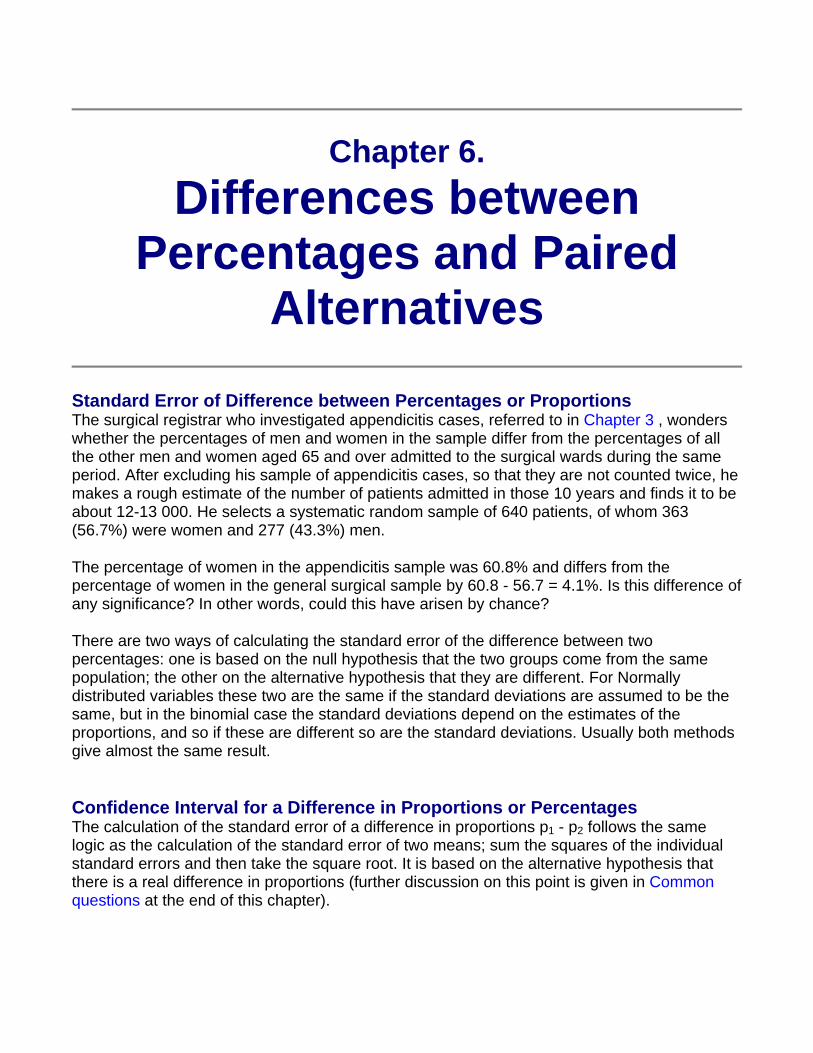
Confidence Interval for a Difference in Proportions or Percentages The calculation of the standard error of a difference in proportions p1 - p2 follows the same logic as the calculation of the standard error of two means; sum the squares of the individual standard errors and then take the square root. It is based on the alternative hypothesis that there is a real difference in proportions (further discussion on this point is given in Common questions at the end of this chapter).

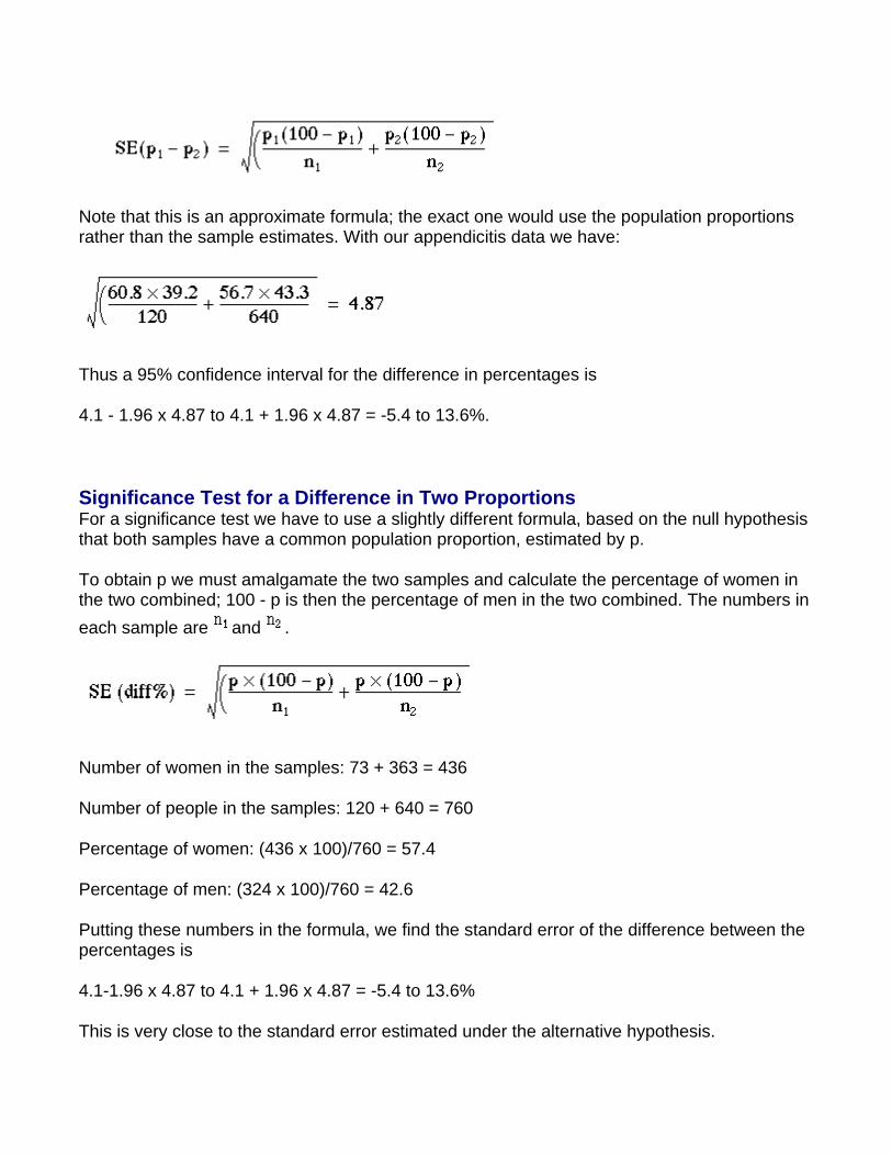
Note that this is an approximate formula; the exact one would use the population proportions rather than the sample estimates. With our appendicitis data we have:

Thus a 95% confidence interval for the difference in percentages is

4.1 - 1.96 x 4.87 to 4.1 + 1.96 x 4.87 = -5.4 to 13.6%.

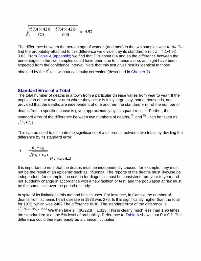
Significance Test for a Difference in Two Proportions For a significance test we have to use a slightly different formula, based on the null hypothesis that both samples have a common population proportion, estimated by p.

To obtain p we must amalgamate the two samples and calculate the percentage of women in the two combined; 100 - p is then the percentage of men in the two combined. The numbers in each sample are and .

Number of women in the samples: 73 + 363 = 436

Number of people in the samples: 120 + 640 = 760

Percentage of women: (436 x 100)/760 = 57.4

Percentage of men: (324 x 100)/760 = 42.6

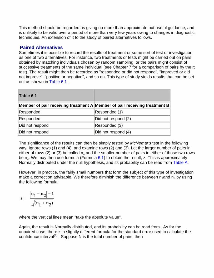
Putting these numbers in the formula, we find the standard error of the difference between the percentages is

4.1-1.96 x 4.87 to 4.1 + 1.96 x 4.87 = -5.4 to 13.6%

This is very close to the standard error estimated under the alternative hypothesis.

The difference between the percentage of women (and men) in the two samples was 4.1%. To find the probability attached to this difference we divide it by its standard error: z = 4.1/4.92 = 0.83. From Table A (appendix) we find that P is about 0.4 and so the difference between the percentages in the two samples could have been due to chance alone, as might have been expected from the confidence interval. Note that this test gives results identical to those

obtained by the test without continuity correction (described in Chapter 7).

Standard Error of a Total The total number of deaths in a town from a particular disease varies from year to year. If the population of the town or area where they occur is fairly large, say, some thousands, and provided that the deaths are independent of one another, the standard error of the number of deaths from a specified cause is given approximately by its square root, Further, the standard error of the difference between two numbers of deaths, and , can be taken as

This can be used to estimate the significance of a difference between two totals by dividing the difference by its standard error:

(Formula 6.1)

It is important to note that the deaths must be independently caused; for example, they must not be the result of an epidemic such as influenza. The reports of the deaths must likewise be independent; for example, the criteria for diagnosis must be consistent from year to year and not suddenly change in accordance with a new fashion or test, and the population at risk must be the same size over the period of study.

In spite of its limitations this method has its uses. For instance, in Carlisle the number of deaths from ischemic heart disease in 1973 was 276. Is this significantly higher than the total for 1972, which was 246? The difference is 30. The standard error of the difference is

We then take z = 30/22.8 = 1.313. This is clearly much less than 1.96 times the standard error at the 5% level of probability. Reference to Table A shows that P = 0.2. The difference could therefore easily be a chance fluctuation.

This method should be regarded as giving no more than approximate but useful guidance, and is unlikely to be valid over a period of more than very few years owing to changes in diagnostic techniques. An extension of it to the study of paired alternatives follows.

Paired Alternatives Sometimes it is possible to record the results of treatment or some sort of test or investigation as one of two alternatives. For instance, two treatments or tests might be carried out on pairs obtained by matching individuals chosen by random sampling, or the pairs might consist of successive treatments of the same individual (see Chapter 7 for a comparison of pairs by the tt test). The result might then be recorded as "responded or did not respond", "improved or did not improve", "positive or negative", and so on. This type of study yields results that can be set out as shown in Table 6.1.

Table 6.1

Member of pair receiving treatment A Member of pair receiving treatment B Responded Responded (1) Responded Did not respond (2) Did not respond Responded (3) Did not respond Did not respond (4)

The significance of the results can then be simply tested by McNemar's test in the following way. Ignore rows (1) and (4), and examine rows (2) and (3). Let the larger number of pairs in either of rows (2) or (3) be called n1 and the smaller number of pairs in either of those two rows be n2. We may then use formula (Formula 6.1) to obtain the result, z. This is approximately Normally distributed under the null hypothesis, and its probability can be read from Table A.

However, in practice, the fairly small numbers that form the subject of this type of investigation make a correction advisable. We therefore diminish the difference between n1and n2 by using the following formula:

where the vertical lines mean "take the absolute value".

Again, the result is Normally distributed, and its probability can be read from . As for the unpaired case, there is a slightly different formula for the standard error used to calculate the confidence interval(1). Suppose N is the total number of pairs, then

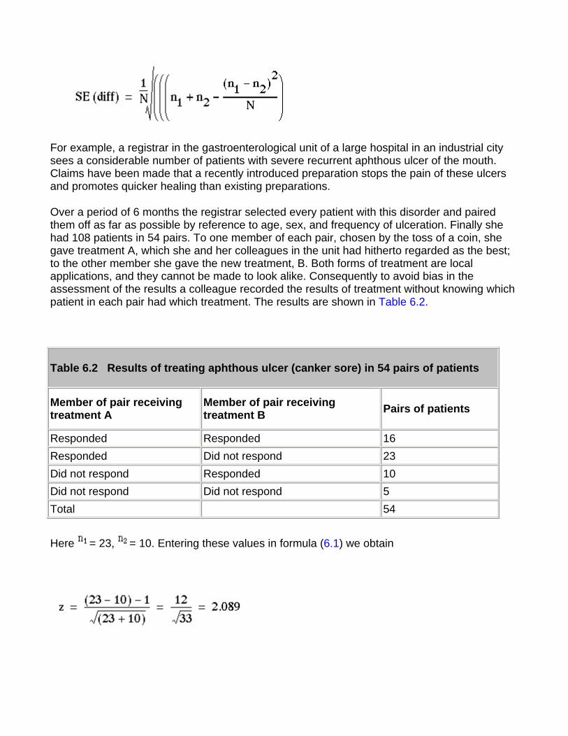
For example, a registrar in the gastroenterological unit of a large hospital in an industrial city sees a considerable number of patients with severe recurrent aphthous ulcer of the mouth. Claims have been made that a recently introduced preparation stops the pain of these ulcers and promotes quicker healing than existing preparations.

Over a period of 6 months the registrar selected every patient with this disorder and paired them off as far as possible by reference to age, sex, and frequency of ulceration. Finally she had 108 patients in 54 pairs. To one member of each pair, chosen by the toss of a coin, she gave treatment A, which she and her colleagues in the unit had hitherto regarded as the best; to the other member she gave the new treatment, B. Both forms of treatment are local applications, and they cannot be made to look alike. Consequently to avoid bias in the assessment of the results a colleague recorded the results of treatment without knowing which patient in each pair had which treatment. The results are shown in Table 6.2.

Table 6.2 Results of treating aphthous ulcer (canker sore) in 54 pairs of patients

Member of pair receiving treatment A

Member of pair receiving treatment B Pairs of patients

Responded Responded 16 Responded Did not respond 23 Did not respond Responded 10 Did not respond Did not respond 5 Total 54

Here = 23, = 10. Entering these values in formula (6.1) we obtain

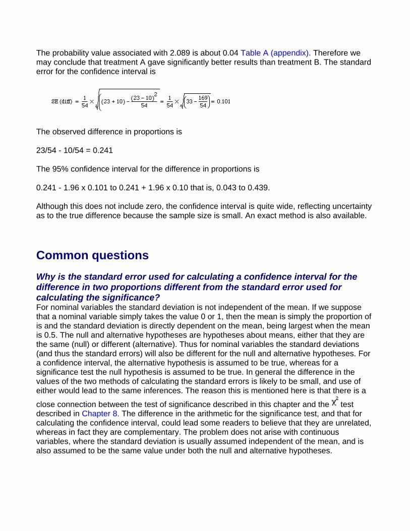
The probability value associated with 2.089 is about 0.04 Table A (appendix). Therefore we may conclude that treatment A gave significantly better results than treatment B. The standard error for the confidence interval is

The observed difference in proportions is

23/54 - 10/54 = 0.241

The 95% confidence interval for the difference in proportions is

0.241 - 1.96 x 0.101 to 0.241 + 1.96 x 0.10 that is, 0.043 to 0.439.

Although this does not include zero, the confidence interval is quite wide, reflecting uncertainty as to the true difference because the sample size is small. An exact method is also available.

Common questions

Why is the standard error used for calculating a confidence interval for the difference in two proportions different from the standard error used for calculating the significance? For nominal variables the standard deviation is not independent of the mean. If we suppose that a nominal variable simply takes the value 0 or 1, then the mean is simply the proportion of is and the standard deviation is directly dependent on the mean, being largest when the mean is 0.5. The null and alternative hypotheses are hypotheses about means, either that they are the same (null) or different (alternative). Thus for nominal variables the standard deviations (and thus the standard errors) will also be different for the null and alternative hypotheses. For a confidence interval, the alternative hypothesis is assumed to be true, whereas for a significance test the null hypothesis is assumed to be true. In general the difference in the values of the two methods of calculating the standard errors is likely to be small, and use of either would lead to the same inferences. The reason this is mentioned here is that there is a

close connection between the test of significance described in this chapter and the test described in Chapter 8. The difference in the arithmetic for the significance test, and that for calculating the confidence interval, could lead some readers to believe that they are unrelated, whereas in fact they are complementary. The problem does not arise with continuous variables, where the standard deviation is usually assumed independent of the mean, and is also assumed to be the same value under both the null and alternative hypotheses.

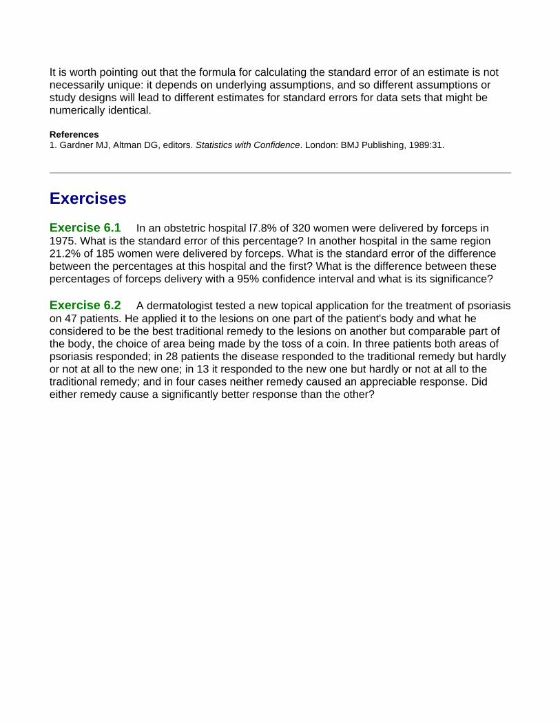
It is worth pointing out that the formula for calculating the standard error of an estimate is not necessarily unique: it depends on underlying assumptions, and so different assumptions or study designs will lead to different estimates for standard errors for data sets that might be numerically identical.

References 1. Gardner MJ, Altman DG, editors. Statistics with Confidence. London: BMJ Publishing, 1989:31.

Exercises

Exercise 6.1 In an obstetric hospital l7.8% of 320 women were delivered by forceps in 1975. What is the standard error of this percentage? In another hospital in the same region 21.2% of 185 women were delivered by forceps. What is the standard error of the difference between the percentages at this hospital and the first? What is the difference between these percentages of forceps delivery with a 95% confidence interval and what is its significance?

Exercise 6.2 A dermatologist tested a new topical application for the treatment of psoriasis on 47 patients. He applied it to the lesions on one part of the patient's body and what he considered to be the best traditional remedy to the lesions on another but comparable part of the body, the choice of area being made by the toss of a coin. In three patients both areas of psoriasis responded; in 28 patients the disease responded to the traditional remedy but hardly or not at all to the new one; in 13 it responded to the new one but hardly or not at all to the traditional remedy; and in four cases neither remedy caused an appreciable response. Did either remedy cause a significantly better response than the other?

Chapter 7. The t Tests

Previously we have considered how to test the null hypothesis that there is no difference between the mean of a sample and the population mean, and no difference between the means of two samples. We obtained the difference between the means by subtraction, and then divided this difference by the standard error of the difference. If the difference is 196 times its standard error, or more, it is likely to occur by chance with a frequency of only 1 in 20, or less.

With small samples, where more chance variation must be allowed for, these ratios are not entirely accurate because the uncertainty in estimating the standard error has been ignored. Some modification of the procedure of dividing the difference by its standard error is needed, and the technique to use is the t test. Its foundations were laid by WS Gosset, writing under the pseudonym "Student" so that it is sometimes known as Student's t test. The procedure does not differ greatly from the one used for large samples, but is preferable when the number of observations is less than 60, and certainly when they amount to 30 or less.

The application of the t distribution to the following four types of problem will now be considered.

1. The calculation of a confidence interval for a sample mean. 2. The mean and standard deviation of a sample are calculated and a value is postulated

for the mean of the population. How significantly does the sample mean differ from the postulated population mean?

3. The means and standard deviations of two samples are calculated. Could both samples have been taken from the same population?

4. Paired observations are made on two samples (or in succession on one sample). What is the significance of the difference between the means of the two sets of observations?

In each case the problem is essentially the same - namely, to establish multiples of standard errors to which probabilities can be attached. These multiples are the number of times a difference can be divided by its standard error. We have seen that with large samples 1.96 times the standard error has a probability of 5% or less, and 2.576 times the standard error a probability of 1% or less (Table A appendix). With small samples these multiples are larger, and the smaller the sample the larger they become.

Confidence interval for the mean from a small sample A rare congenital disease, Everley's syndrome, generally causes a reduction in concentration

of blood sodium. This is thought to provide a useful diagnostic sign as well as a clue to the efficacy of treatment. Little is known about the subject, but the director of a dermatological department in a London teaching hospital is known to be interested in the disease and has seen more cases than anyone else. Even so, he has seen only 18. The patients were all aged between 20 and 44.

The mean blood sodium concentration of these 18 cases was 115mmol/l, with standard deviation of 12mmol/l. Assuming that blood sodium concentration is Normally distributed what is the 95% confidence interval within which the mean of the total population of such cases may be expected to lie?

The data are set out as follows:

Number of observations 18 Mean blood sodium concentration 115 mmol/l Standard deviation 12 mmo1/l Standard error of mean

To find the 95% confidence interval above and below the mean we now have to find a multiple of the standard error. In large samples we have seen that the multiple is 1.96 (Chapter 4). For small samples we use the Table of t given in Table B (Appendix). As the sample becomes smaller t becomes larger for any particular level of probability. Conversely, as the sample becomes larger t becomes smaller and approaches the values given in Table A, reaching them for infinitely large samples.

Since the size of the sample influences the value of t, the size of the sample is taken into account in relating the value of t to probabilities in the Table. Some useful parts of the full t Table appear in . The left hand column is headed d.f. for "degrees of freedom". The use of these was noted in the calculation of the standard deviation (Chapter 2). In practice the degrees of freedom amount in these circumstances to one less than the number of observations in the sample. With these data we have 18 - 1 = 17 d.f. This is because only 17 observations plus the total number of observations are needed to specify the sample, the 18th being determined by subtraction.

To find the number by which we must multiply the standard error to give the 95% confidence interval we enter Table B at 17 in the left hand column and read across to the column headed 0.05 to discover the number 2.110. The 95% confidence intervals of the mean are now set as follows:

Mean + 2.110 SE to Mean - 2.110 SE

which gives us:

115 - (2.110 x 283) to 115 + 2.110 x 2.83 or 109.03 to 120.97 mmol/l.

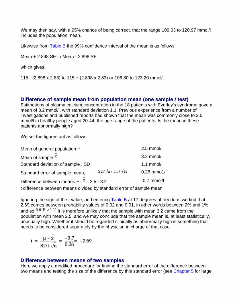
We may then say, with a 95% chance of being correct, that the range 109.03 to 120.97 mmol/l includes the population mean.

Likewise from Table B the 99% confidence interval of the mean is as follows:

Mean + 2.898 SE to Mean - 2.898 SE

which gives:

115 - (2.898 x 2.83) to 115 + (2.898 x 2.83) or 106.80 to 123.20 mmol/l.

Difference of sample mean from population mean (one sample t test) Estimations of plasma calcium concentration in the 18 patients with Everley's syndrome gave a mean of 3.2 mmol/l, with standard deviation 1.1. Previous experience from a number of investigations and published reports had shown that the mean was commonly close to 2.5 mmol/l in healthy people aged 20-44, the age range of the patients. Is the mean in these patients abnormally high?

We set the figures out as follows:

Mean of general population 2.5 mmol/l

Mean of sample 3.2 mmol/l

Standard deviation of sample , SD 1.1 mmol/l

Standard error of sample mean, 0.26 mmo1/l

Difference between means - = 2.5 - 3.2 -0.7 mmol/l

t difference between means divided by standard error of sample mean

Ignoring the sign of the t value, and entering Table B at 17 degrees of freedom, we find that 2.69 comes between probability values of 0.02 and 0.01, in other words between 2% and 1% and so It is therefore unlikely that the sample with mean 3.2 came from the population with mean 2.5, and we may conclude that the sample mean is, at least statistically, unusually high. Whether it should be regarded clinically as abnormally high is something that needs to be considered separately by the physician in charge of that case.

Difference between means of two samples Here we apply a modified procedure for finding the standard error of the difference between two means and testing the size of the difference by this standard error (see Chapter 5 for large

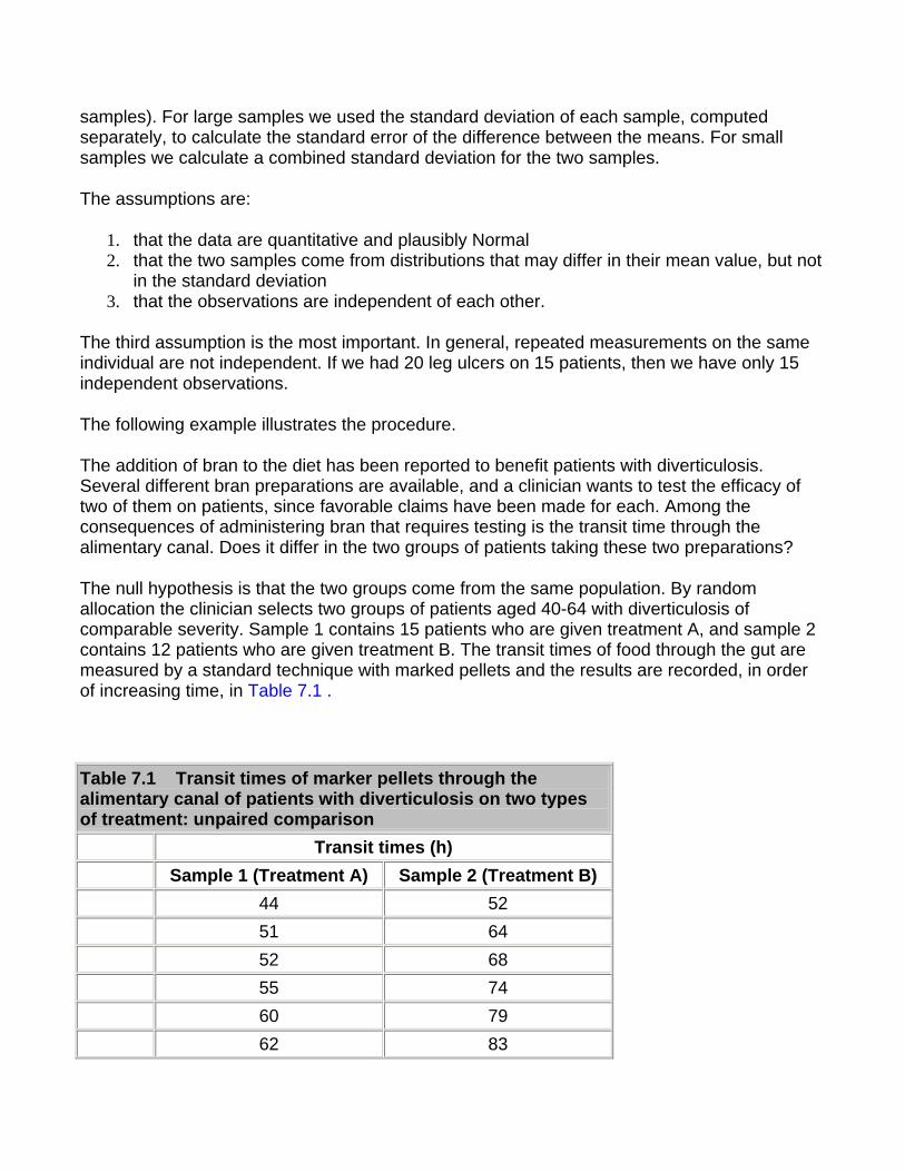
samples). For large samples we used the standard deviation of each sample, computed separately, to calculate the standard error of the difference between the means. For small samples we calculate a combined standard deviation for the two samples.

The assumptions are:

1. that the data are quantitative and plausibly Normal 2. that the two samples come from distributions that may differ in their mean value, but not

in the standard deviation 3. that the observations are independent of each other.

The third assumption is the most important. In general, repeated measurements on the same individual are not independent. If we had 20 leg ulcers on 15 patients, then we have only 15 independent observations.

The following example illustrates the procedure.

The addition of bran to the diet has been reported to benefit patients with diverticulosis. Several different bran preparations are available, and a clinician wants to test the efficacy of two of them on patients, since favorable claims have been made for each. Among the consequences of administering bran that requires testing is the transit time through the alimentary canal. Does it differ in the two groups of patients taking these two preparations?

The null hypothesis is that the two groups come from the same population. By random allocation the clinician selects two groups of patients aged 40-64 with diverticulosis of comparable severity. Sample 1 contains 15 patients who are given treatment A, and sample 2 contains 12 patients who are given treatment B. The transit times of food through the gut are measured by a standard technique with marked pellets and the results are recorded, in order of increasing time, in Table 7.1 .

Table 7.1 Transit times of marker pellets through the alimentary canal of patients with diverticulosis on two types of treatment: unpaired comparison

Transit times (h) Sample 1 (Treatment A) Sample 2 (Treatment B)

44 52 51 64 52 68 55 74 60 79 62 83

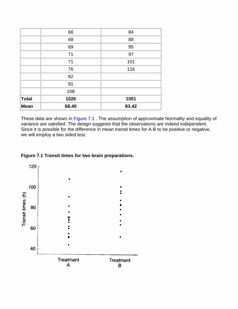
66 84 68 88 69 95 71 97 71 101 76 116 82 91 108 Total 1026 1001 Mean 68.40 83.42

These data are shown in Figure 7.1 . The assumption of approximate Normality and equality of variance are satisfied. The design suggests that the observations are indeed independent. Since it is possible for the difference in mean transit times for A-B to be positive or negative, we will employ a two sided test.

Figure 7.1 Transit times for two brain preparations.

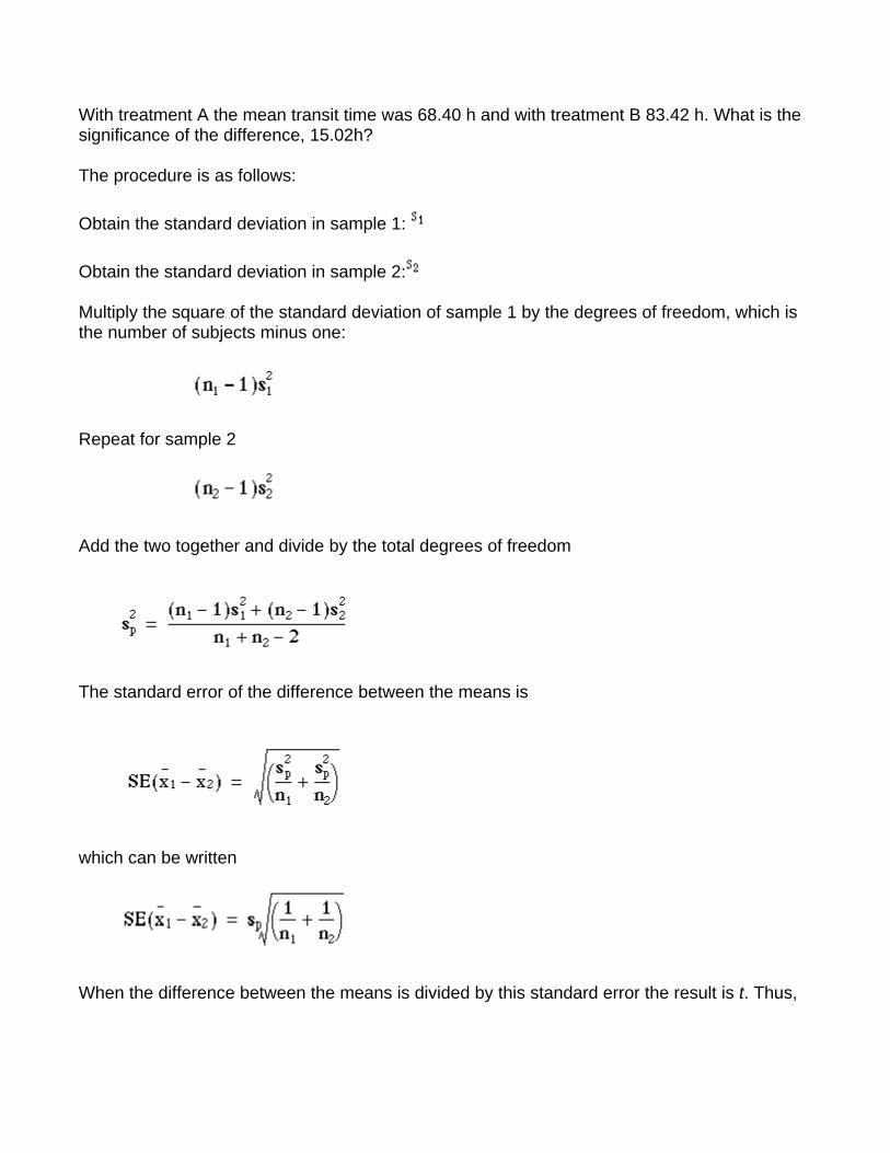
With treatment A the mean transit time was 68.40 h and with treatment B 83.42 h. What is the significance of the difference, 15.02h?

The procedure is as follows:

Obtain the standard deviation in sample 1:

Obtain the standard deviation in sample 2:

Multiply the square of the standard deviation of sample 1 by the degrees of freedom, which is the number of subjects minus one:

Repeat for sample 2

Add the two together and divide by the total degrees of freedom

The standard error of the difference between the means is

which can be written

When the difference between the means is divided by this standard error the result is t. Thus,

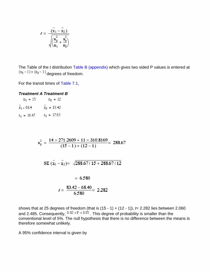
The Table of the t distribution Table B (appendix) which gives two sided P values is entered at degrees of freedom.

For the transit times of Table 7.1,

Treatment A Treatment B

shows that at 25 degrees of freedom (that is (15 - 1) + (12 - 1)), t= 2.282 lies between 2.060 and 2.485. Consequently, . This degree of probability is smaller than the conventional level of 5%. The null hypothesis that there is no difference between the means is therefore somewhat unlikely.

A 95% confidence interval is given by

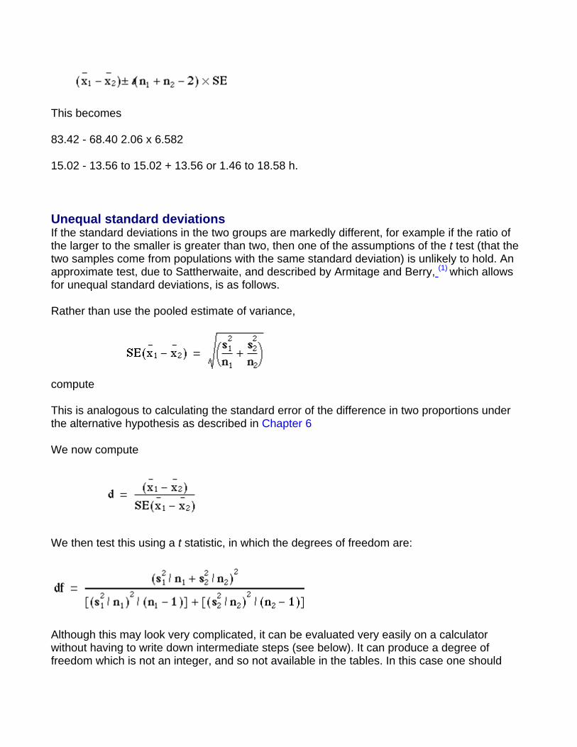
This becomes

83.42 - 68.40 2.06 x 6.582

15.02 - 13.56 to 15.02 + 13.56 or 1.46 to 18.58 h.

Unequal standard deviations If the standard deviations in the two groups are markedly different, for example if the ratio of the larger to the smaller is greater than two, then one of the assumptions of the t test (that the two samples come from populations with the same standard deviation) is unlikely to hold. An approximate test, due to Sattherwaite, and described by Armitage and Berry, (1) which allows for unequal standard deviations, is as follows.

Rather than use the pooled estimate of variance,

compute

This is analogous to calculating the standard error of the difference in two proportions under the alternative hypothesis as described in Chapter 6

We now compute

We then test this using a t statistic, in which the degrees of freedom are:

Although this may look very complicated, it can be evaluated very easily on a calculator without having to write down intermediate steps (see below). It can produce a degree of freedom which is not an integer, and so not available in the tables. In this case one should

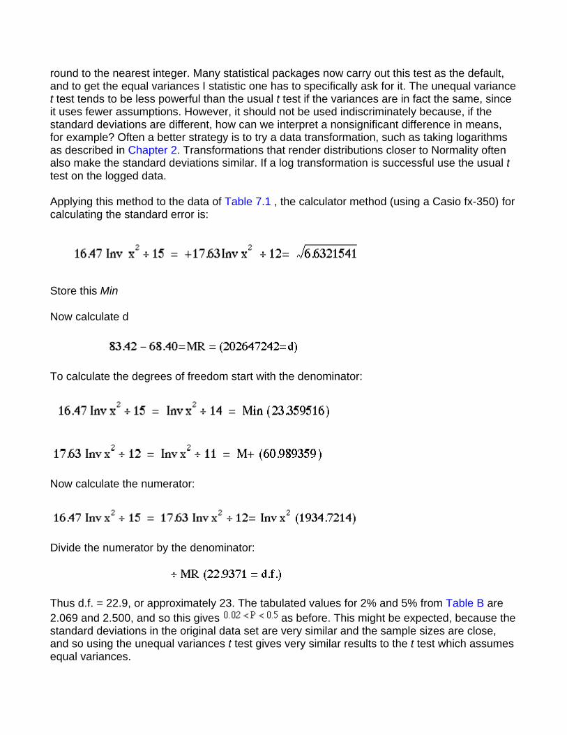
round to the nearest integer. Many statistical packages now carry out this test as the default, and to get the equal variances I statistic one has to specifically ask for it. The unequal variance t test tends to be less powerful than the usual t test if the variances are in fact the same, since it uses fewer assumptions. However, it should not be used indiscriminately because, if the standard deviations are different, how can we interpret a nonsignificant difference in means, for example? Often a better strategy is to try a data transformation, such as taking logarithms as described in Chapter 2. Transformations that render distributions closer to Normality often also make the standard deviations similar. If a log transformation is successful use the usual t test on the logged data.

Applying this method to the data of Table 7.1 , the calculator method (using a Casio fx-350) for calculating the standard error is:

Store this Min

Now calculate d

To calculate the degrees of freedom start with the denominator:

Now calculate the numerator:

Divide the numerator by the denominator:

Thus d.f. = 22.9, or approximately 23. The tabulated values for 2% and 5% from Table B are 2.069 and 2.500, and so this gives as before. This might be expected, because the standard deviations in the original data set are very similar and the sample sizes are close, and so using the unequal variances t test gives very similar results to the t test which assumes equal variances.

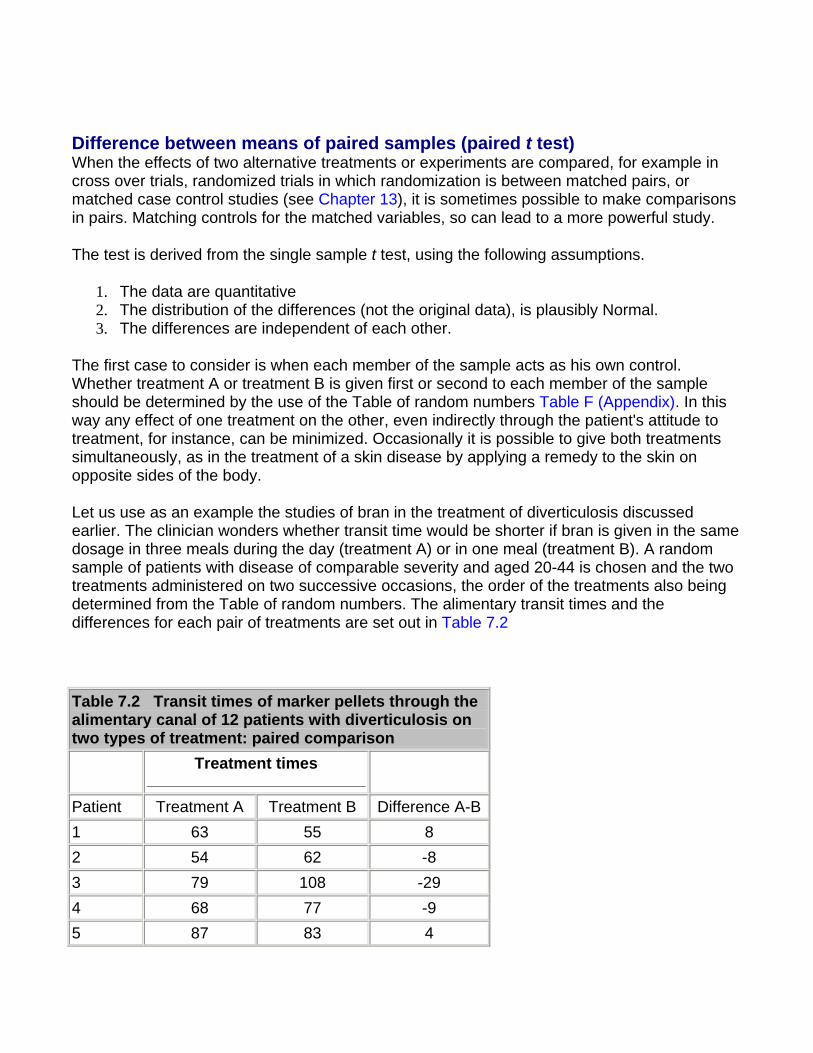
Difference between means of paired samples (paired t test) When the effects of two alternative treatments or experiments are compared, for example in cross over trials, randomized trials in which randomization is between matched pairs, or matched case control studies (see Chapter 13), it is sometimes possible to make comparisons in pairs. Matching controls for the matched variables, so can lead to a more powerful study.

The test is derived from the single sample t test, using the following assumptions.

1. The data are quantitative 2. The distribution of the differences (not the original data), is plausibly Normal. 3. The differences are independent of each other.

The first case to consider is when each member of the sample acts as his own control. Whether treatment A or treatment B is given first or second to each member of the sample should be determined by the use of the Table of random numbers Table F (Appendix). In this way any effect of one treatment on the other, even indirectly through the patient's attitude to treatment, for instance, can be minimized. Occasionally it is possible to give both treatments simultaneously, as in the treatment of a skin disease by applying a remedy to the skin on opposite sides of the body.

Let us use as an example the studies of bran in the treatment of diverticulosis discussed earlier. The clinician wonders whether transit time would be shorter if bran is given in the same dosage in three meals during the day (treatment A) or in one meal (treatment B). A random sample of patients with disease of comparable severity and aged 20-44 is chosen and the two treatments administered on two successive occasions, the order of the treatments also being determined from the Table of random numbers. The alimentary transit times and the differences for each pair of treatments are set out in Table 7.2

Table 7.2 Transit times of marker pellets through the alimentary canal of 12 patients with diverticulosis on two types of treatment: paired comparison

Treatment times

Patient Treatment A Treatment B Difference A-B 1 63 55 8 2 54 62 -8 3 79 108 -29 4 68 77 -9 5 87 83 4

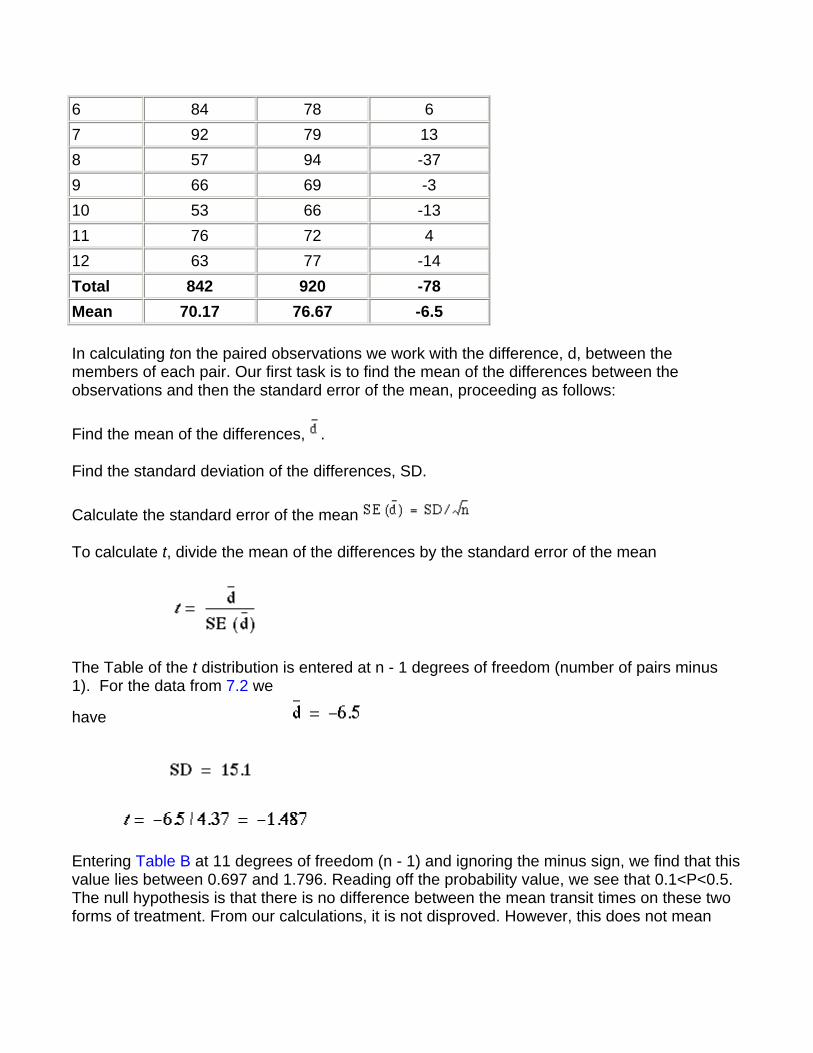
6 84 78 6 7 92 79 13 8 57 94 -37 9 66 69 -3 10 53 66 -13 11 76 72 4 12 63 77 -14 Total 842 920 -78 Mean 70.17 76.67 -6.5

In calculating ton the paired observations we work with the difference, d, between the members of each pair. Our first task is to find the mean of the differences between the observations and then the standard error of the mean, proceeding as follows:

Find the mean of the differences, .

Find the standard deviation of the differences, SD.

Calculate the standard error of the mean

To calculate t, divide the mean of the differences by the standard error of the mean

The Table of the t distribution is entered at n - 1 degrees of freedom (number of pairs minus 1). For the data from 7.2 we

have

Entering Table B at 11 degrees of freedom (n - 1) and ignoring the minus sign, we find that this value lies between 0.697 and 1.796. Reading off the probability value, we see that 0.1<P<0.5. The null hypothesis is that there is no difference between the mean transit times on these two forms of treatment. From our calculations, it is not disproved. However, this does not mean

that the two treatments are equivalent. To help us decide this we calculate the confidence interval.

A 95% confidence interval for the mean difference is given by

In this case t11 at P = 0.05 is 2.201 (Table B) and so the 95% confidence interval is:

-6.5 - 2.201 x 4.37 to -6.5 + 2.201 x 4.37 h. or -16.1 to 3.1h.

This is quite wide, so we cannot really conclude that the two preparations are equivalent, and should look to a larger study.

The second case of a paired comparison to consider is when two samples are chosen and each member of sample 1 is paired with one member of sample 2, as in a matched case control study. As the aim is to test the difference, if any, between two types of treatment, the choice of members for each pair is designed to make them as alike as possible. The more alike they are, the more apparent will be any differences due to treatment, because they will not be confused with differences in the results caused by disparities between members of the pair. The likeness within the pairs applies to attributes relating to the study in question. For instance, in a test for a drug reducing blood pressure the color of the patients' eyes would probably be irrelevant, but their resting diastolic blood pressure could well provide a basis for selecting the pairs. Another (perhaps related) basis is the prognosis for the disease in patients: in general, patients with a similar prognosis are best paired. Whatever criteria are chosen, it is essential that the pairs are constructed before the treatment is given, for the pairing must be uninfluenced by knowledge of the effects of treatment.

Further methods Suppose we had a clinical trial with more than two treatments. It is not valid to compare each treatment with each other treatment using t tests because the overall type I error rate will be bigger than the conventional level set for each individual test. A method of controlling for this to use a one way analysis of variance.(2)

Common questions

Should I test my data for Normality before using the t test? It would seem logical that, because the t test assumes Normality, one should test for Normality first. The problem is that the test for Normality is dependent on the sample size. With a small

sample a non-significant result does not mean that the data come from a Normal distribution. On the other hand, with a large sample, a significant result does not mean that we could not use the t test, because the t test is robust to moderate departures from Normality - that is, the P value obtained can be validly interpreted. There is something illogical about using one significance test conditional on the results of another significance test. In general it is a matter of knowing and looking at the data. One can "eyeball" the data and if the distributions are not extremely skewed, and particularly if (for the two sample t test) the numbers of observations are similar in the two groups, then the t test will be valid. The main problem is often that outliers will inflate the standard deviations and render the test less sensitive. Also, it is not generally appreciated that if the data originate from a randomized controlled trial, then the process of randomization will ensure the validity of the t test, irrespective of the original distribution of the data.

Should I test for equality of the standard deviations before using the usual t test? The same argument prevails here as for the previous question about Normality. The test for equality of variances is dependent on the sample size. A rule of thumb is that if the ratio of the larger to smaller standard deviation is greater than two, then the unequal variance test should be used. With a computer one can easily do both the equal and unequal variance t test and see if the answers differ.

Why should I use a paired test if my data are paired? What happens if I don't? Pairing provides information about an experiment, and the more information that can be provided in the analysis the more sensitive the test. One of the major sources of variability is between subjects variability. By repeating measures within subjects, each subject acts as its own control, and the between subjects variability is removed. In general this means that if there is a true difference between the pairs the paired test is more likely to pick it up: it is more powerful. When the pairs are generated by matching the matching criteria may not be important. In this case, the paired and unpaired tests should give similar results.

References 1. Armitage P, Berry G. Statistical Methods in Medical Research. 3rd ed. Oxford: Blackwell Scientific Publications, 1994:112-13. 2. Armitage P, Berry G. Statistical Methods in Medical Research. 3rd ed. Oxford: Blackwell Scientific Publications, 1994:207-14.

Exercises

Exercise 7.1 In 22 patients with an unusual liver disease the plasma alkaline phosphatase was found by a certain laboratory to have a mean value of 39 King-Armstrong units, standard deviation 3.4 units. What is the 95% confidence interval within which the mean of the

population of such cases whose specimens come to the same laboratory may be expected to lie?

Exercise 7.2 In the 18 patients with Everley's syndrome the mean level of plasma phosphate was 1.7 mmol/l, standard deviation 0.8. If the mean level in the general population is taken as 1.2 mmol/l, what is the significance of the difference between that mean and the mean of these 18 patients?

Exercise 7.3 In two wards for elderly women in a geriatric hospital the following levels of hemoglobin were found:

Ward A: 12.2, 11.1, 14.0, 11.3, 10.8, 12.5, 12.2, 11.9, 13.6, 12.7, 13.4, 13.7 g/dl;

Ward B: 11.9, 10.7, 12.3, 13.9, 11.1, 11.2, 13.3, 11.4, 12.0, 11.1 g/dl.

What is the difference between the mean levels in the two wards, and what is its significance? What is the 95% confidence interval for the difference in treatments?

Exercise 7.4 A new treatment for varicose ulcer is compared with a standard treatment on ten matched pairs of patients, where treatment between pairs is decided using random numbers. The outcome is the number of days from start of treatment to healing of ulcer. One doctor is responsible for treatment and a second doctor assesses healing without knowing which treatment each patient had. The following treatment times were recorded.

Standard treatment: 35, 104, 27, 53, 72, 64, 97, 121, 86, 41 days;

New treatment: 27, 52, 46, 33, 37, 82, 51, 92, 68, 62 days.

What are the mean difference in the healing time, the value of t, the number of degrees of freedom, and the probability? What is the 95% confidence interval for the difference?

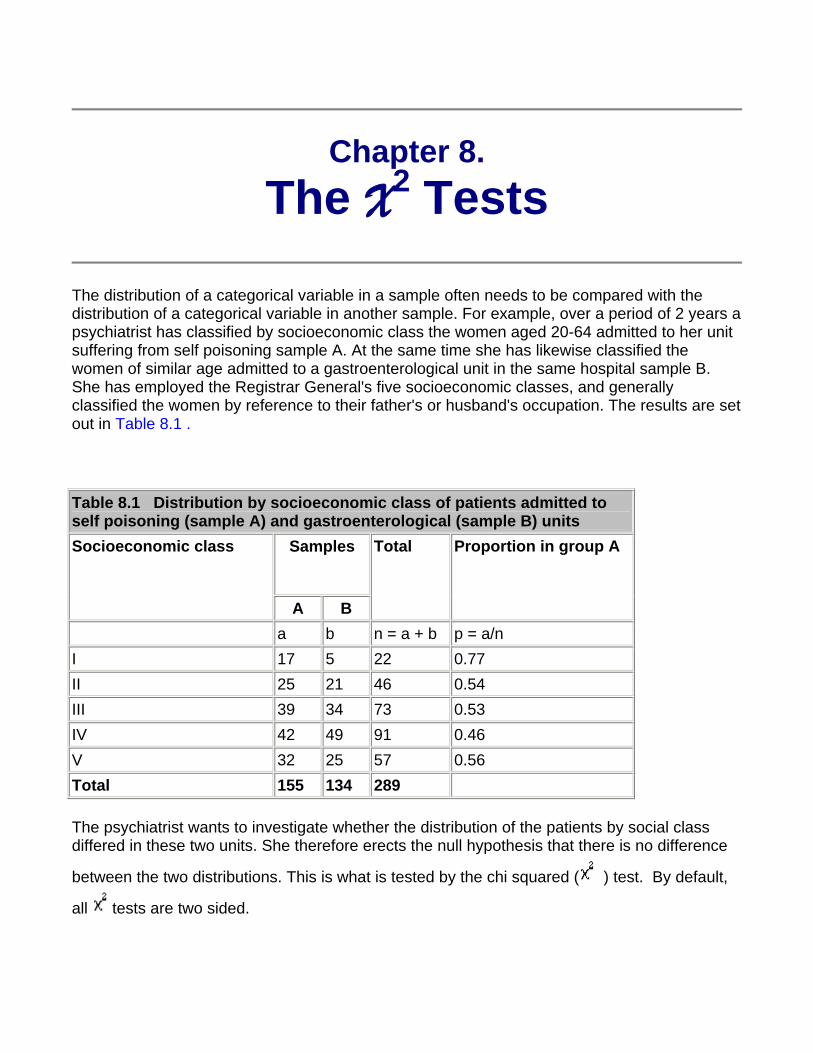
Chapter 8. The X2 Tests

The distribution of a categorical variable in a sample often needs to be compared with the distribution of a categorical variable in another sample. For example, over a period of 2 years a psychiatrist has classified by socioeconomic class the women aged 20-64 admitted to her unit suffering from self poisoning sample A. At the same time she has likewise classified the women of similar age admitted to a gastroenterological unit in the same hospital sample B. She has employed the Registrar General's five socioeconomic classes, and generally classified the women by reference to their father's or husband's occupation. The results are set out in Table 8.1 .

Table 8.1 Distribution by socioeconomic class of patients admitted to self poisoning (sample A) and gastroenterological (sample B) units

Samples

Socioeconomic class

A B

Total Proportion in group A

a b n = a + b p = a/n I 17 5 22 0.77 II 25 21 46 0.54 III 39 34 73 0.53 IV 42 49 91 0.46 V 32 25 57 0.56 Total 155 134 289

The psychiatrist wants to investigate whether the distribution of the patients by social class differed in these two units. She therefore erects the null hypothesis that there is no difference

between the two distributions. This is what is tested by the chi squared ( ) test. By default,

all tests are two sided.

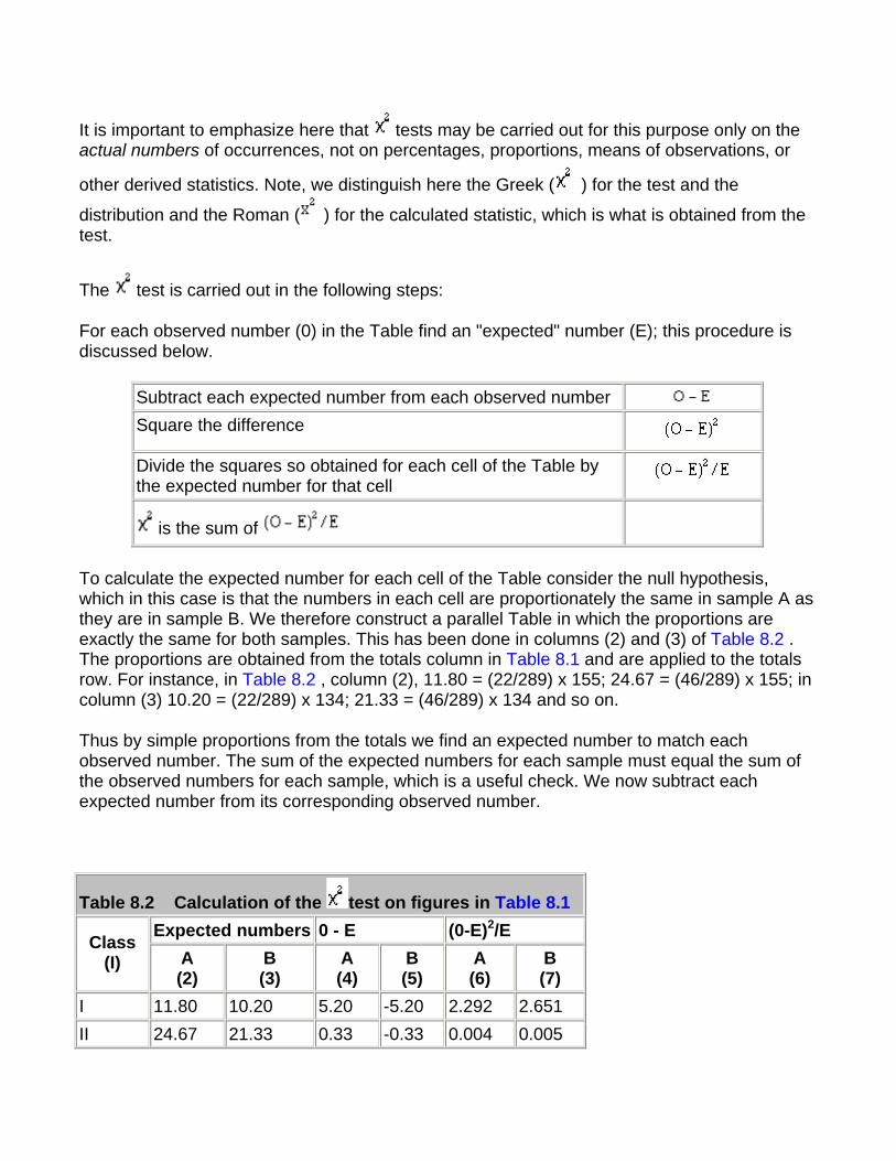
It is important to emphasize here that tests may be carried out for this purpose only on the actual numbers of occurrences, not on percentages, proportions, means of observations, or

other derived statistics. Note, we distinguish here the Greek ( ) for the test and the

distribution and the Roman ( ) for the calculated statistic, which is what is obtained from the test.

The test is carried out in the following steps:

For each observed number (0) in the Table find an "expected" number (E); this procedure is discussed below.

Subtract each expected number from each observed number Square the difference

Divide the squares so obtained for each cell of the Table by the expected number for that cell

is the sum of

To calculate the expected number for each cell of the Table consider the null hypothesis, which in this case is that the numbers in each cell are proportionately the same in sample A as they are in sample B. We therefore construct a parallel Table in which the proportions are exactly the same for both samples. This has been done in columns (2) and (3) of Table 8.2 . The proportions are obtained from the totals column in Table 8.1 and are applied to the totals row. For instance, in Table 8.2 , column (2), 11.80 = (22/289) x 155; 24.67 = (46/289) x 155; in column (3) 10.20 = (22/289) x 134; 21.33 = (46/289) x 134 and so on.

Thus by simple proportions from the totals we find an expected number to match each observed number. The sum of the expected numbers for each sample must equal the sum of the observed numbers for each sample, which is a useful check. We now subtract each expected number from its corresponding observed number.

Table 8.2 Calculation of the test on figures in Table 8.1 Expected numbers 0 - E (0-E)2/E Class

(I) A (2)

B (3)

A (4)

B (5)

A (6)

B (7)

I 11.80 10.20 5.20 -5.20 2.292 2.651 II 24.67 21.33 0.33 -0.33 0.004 0.005

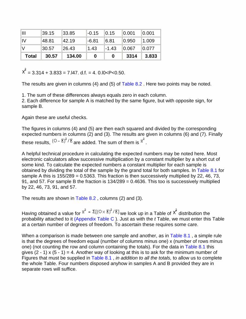
III 39.15 33.85 -0.15 0.15 0.001 0.001 IV 48.81 42.19 -6.81 6.81 0.950 1.009 V 30.57 26.43 1.43 -1.43 0.067 0.077

Total 30.57 134.00 0 0 3314 3.833

= 3.314 + 3.833 = 7.l47. d.f. = 4. 0.l0<P<0.50.

The results are given in columns (4) and (5) of Table 8.2 . Here two points may be noted.

1. The sum of these differences always equals zero in each column. 2. Each difference for sample A is matched by the same figure, but with opposite sign, for sample B.

Again these are useful checks.

The figures in columns (4) and (5) are then each squared and divided by the corresponding expected numbers in columns (2) and (3). The results are given in columns (6) and (7). Finally

these results, are added. The sum of them is .

A helpful technical procedure in calculating the expected numbers may be noted here. Most electronic calculators allow successive multiplication by a constant multiplier by a short cut of some kind. To calculate the expected numbers a constant multiplier for each sample is obtained by dividing the total of the sample by the grand total for both samples. In Table 8.1 for sample A this is 155/289 = 0.5363. This fraction is then successively multiplied by 22, 46, 73, 91, and 57. For sample B the fraction is 134/289 = 0.4636. This too is successively multiplied by 22, 46, 73, 91, and 57.

The results are shown in Table 8.2 , columns (2) and (3).

Having obtained a value for we look up in a Table of distribution the probability attached to it (Appendix Table C ). Just as with the t Table, we must enter this Table at a certain number of degrees of freedom. To ascertain these requires some care.

When a comparison is made between one sample and another, as in Table 8.1 , a simple rule is that the degrees of freedom equal (number of columns minus one) x (number of rows minus one) (not counting the row and column containing the totals). For the data in Table 8.1 this gives (2 - 1) x (5 - 1) = 4. Another way of looking at this is to ask for the minimum number of Figures that must be supplied in Table 8.1 , in addition to all the totals, to allow us to complete the whole Table. Four numbers disposed anyhow in samples A and B provided they are in separate rows will suffice.

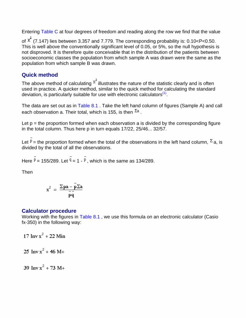
Entering Table C at four degrees of freedom and reading along the row we find that the value

of (7.147) lies between 3.357 and 7.779. The corresponding probability is: 0.10<P<0.50. This is well above the conventionally significant level of 0.05, or 5%, so the null hypothesis is not disproved. It is therefore quite conceivable that in the distribution of the patients between socioeconomic classes the population from which sample A was drawn were the same as the population from which sample B was drawn.

Quick method The above method of calculating illustrates the nature of the statistic clearly and is often used in practice. A quicker method, similar to the quick method for calculating the standard deviation, is particularly suitable for use with electronic calculators(1).

The data are set out as in Table 8.1 . Take the left hand column of figures (Sample A) and call each observation a. Their total, which is 155, is then .

Let p = the proportion formed when each observation a is divided by the corresponding figure in the total column. Thus here p in turn equals 17/22, 25/46... 32/57.

Let = the proportion formed when the total of the observations in the left hand column, a, is divided by the total of all the observations.

Here = 155/289. Let = 1 - , which is the same as 134/289.

Then

Calculator procedure Working with the figures in Table 8.1 , we use this formula on an electronic calculator (Casio fx-350) in the following way:

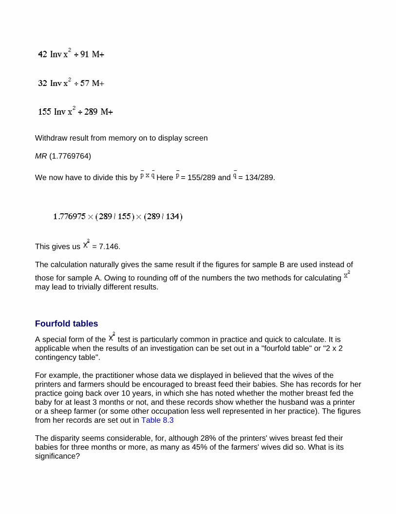
Withdraw result from memory on to display screen

MR (1.7769764)

We now have to divide this by Here = 155/289 and = 134/289.

This gives us = 7.146.

The calculation naturally gives the same result if the figures for sample B are used instead of

those for sample A. Owing to rounding off of the numbers the two methods for calculating may lead to trivially different results.

Fourfold tables

A special form of the test is particularly common in practice and quick to calculate. It is applicable when the results of an investigation can be set out in a "fourfold table" or "2 x 2 contingency table".

For example, the practitioner whose data we displayed in believed that the wives of the printers and farmers should be encouraged to breast feed their babies. She has records for her practice going back over 10 years, in which she has noted whether the mother breast fed the baby for at least 3 months or not, and these records show whether the husband was a printer or a sheep farmer (or some other occupation less well represented in her practice). The figures from her records are set out in Table 8.3

The disparity seems considerable, for, although 28% of the printers' wives breast fed their babies for three months or more, as many as 45% of the farmers' wives did so. What is its significance?

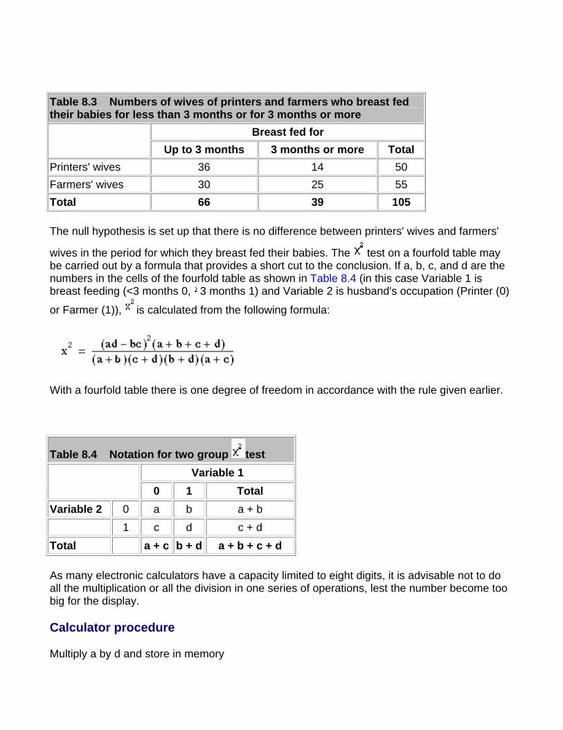
Table 8.3 Numbers of wives of printers and farmers who breast fed their babies for less than 3 months or for 3 months or more

Breast fed for Up to 3 months 3 months or more Total

Printers' wives 36 14 50 Farmers' wives 30 25 55 Total 66 39 105

The null hypothesis is set up that there is no difference between printers' wives and farmers'

wives in the period for which they breast fed their babies. The test on a fourfold table may be carried out by a formula that provides a short cut to the conclusion. If a, b, c, and d are the numbers in the cells of the fourfold table as shown in Table 8.4 (in this case Variable 1 is breast feeding (<3 months 0, 3 months 1) and Variable 2 is husband's occupation (Printer (0)

or Farmer (1)), is calculated from the following formula:

With a fourfold table there is one degree of freedom in accordance with the rule given earlier.

Table 8.4 Notation for two group test Variable 1

0 1 Total Variable 2 0 a b a + b 1 c d c + d

Total a + c b + d a + b + c + d

As many electronic calculators have a capacity limited to eight digits, it is advisable not to do all the multiplication or all the division in one series of operations, lest the number become too big for the display.

Calculator procedure

Multiply a by d and store in memory

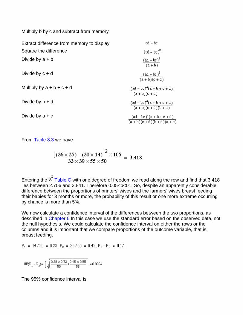
Multiply b by c and subtract from memory

Extract difference from memory to display Square the difference Divide by a + b

Divide by c + d

Multiply by a + b + c + d

Divide by b + d

Divide by a + c

From Table 8.3 we have

Entering the Table C with one degree of freedom we read along the row and find that 3.418 lies between 2.706 and 3.841. Therefore 0.05<p<01. So, despite an apparently considerable difference between the proportions of printers' wives and the farmers' wives breast feeding their babies for 3 months or more, the probability of this result or one more extreme occurring by chance is more than 5%.

We now calculate a confidence interval of the differences between the two proportions, as described in Chapter 6 In this case we use the standard error based on the observed data, not the null hypothesis. We could calculate the confidence interval on either the rows or the columns and it is important that we compare proportions of the outcome variable, that is, breast feeding.

The 95% confidence interval is

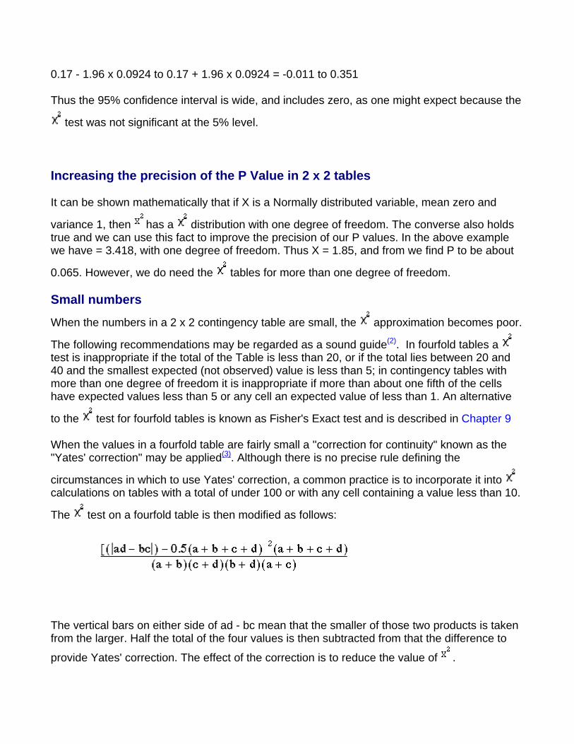
0.17 - 1.96 x 0.0924 to 0.17 + 1.96 x 0.0924 = -0.011 to 0.351

Thus the 95% confidence interval is wide, and includes zero, as one might expect because the

test was not significant at the 5% level.

Increasing the precision of the P Value in 2 x 2 tables

It can be shown mathematically that if X is a Normally distributed variable, mean zero and

variance 1, then has a distribution with one degree of freedom. The converse also holds true and we can use this fact to improve the precision of our P values. In the above example we have = 3.418, with one degree of freedom. Thus X = 1.85, and from we find P to be about

0.065. However, we do need the tables for more than one degree of freedom.

Small numbers

When the numbers in a 2 x 2 contingency table are small, the approximation becomes poor.

The following recommendations may be regarded as a sound guide(2). In fourfold tables a test is inappropriate if the total of the Table is less than 20, or if the total lies between 20 and 40 and the smallest expected (not observed) value is less than 5; in contingency tables with more than one degree of freedom it is inappropriate if more than about one fifth of the cells have expected values less than 5 or any cell an expected value of less than 1. An alternative

to the test for fourfold tables is known as Fisher's Exact test and is described in Chapter 9

When the values in a fourfold table are fairly small a ''correction for continuity" known as the "Yates' correction" may be applied(3). Although there is no precise rule defining the

circumstances in which to use Yates' correction, a common practice is to incorporate it into calculations on tables with a total of under 100 or with any cell containing a value less than 10.

The test on a fourfold table is then modified as follows:

The vertical bars on either side of ad - bc mean that the smaller of those two products is taken from the larger. Half the total of the four values is then subtracted from that the difference to

provide Yates' correction. The effect of the correction is to reduce the value of .

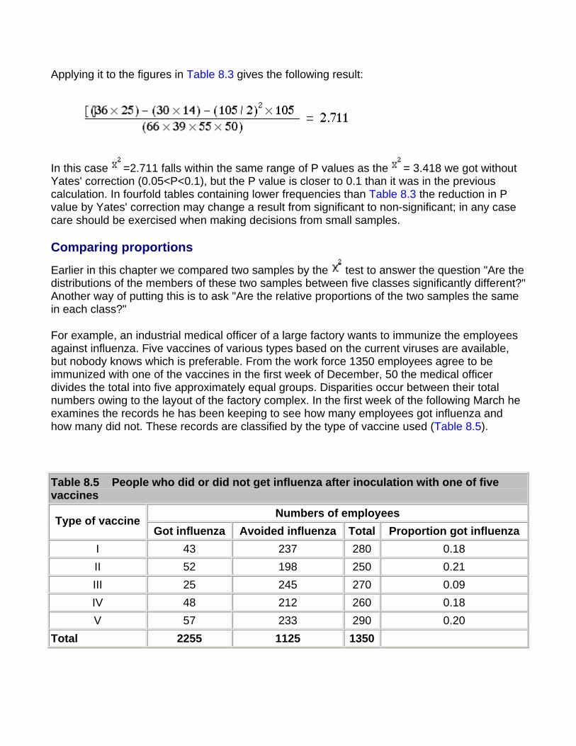
Applying it to the figures in Table 8.3 gives the following result:

In this case =2.711 falls within the same range of P values as the = 3.418 we got without Yates' correction (0.05<P<0.1), but the P value is closer to 0.1 than it was in the previous calculation. In fourfold tables containing lower frequencies than Table 8.3 the reduction in P value by Yates' correction may change a result from significant to non-significant; in any case care should be exercised when making decisions from small samples.

Comparing proportions

Earlier in this chapter we compared two samples by the test to answer the question "Are the distributions of the members of these two samples between five classes significantly different?" Another way of putting this is to ask "Are the relative proportions of the two samples the same in each class?"

For example, an industrial medical officer of a large factory wants to immunize the employees against influenza. Five vaccines of various types based on the current viruses are available, but nobody knows which is preferable. From the work force 1350 employees agree to be immunized with one of the vaccines in the first week of December, 50 the medical officer divides the total into five approximately equal groups. Disparities occur between their total numbers owing to the layout of the factory complex. In the first week of the following March he examines the records he has been keeping to see how many employees got influenza and how many did not. These records are classified by the type of vaccine used (Table 8.5).

Table 8.5 People who did or did not get influenza after inoculation with one of five vaccines

Numbers of employees Type of vaccine Got influenza Avoided influenza Total Proportion got influenza

I 43 237 280 0.18 II 52 198 250 0.21 III 25 245 270 0.09 IV 48 212 260 0.18 V 57 233 290 0.20

Total 2255 1125 1350

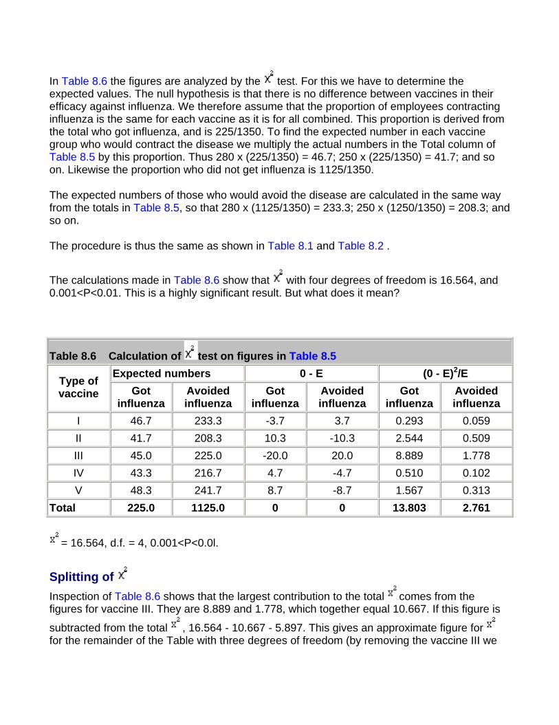
In Table 8.6 the figures are analyzed by the test. For this we have to determine the expected values. The null hypothesis is that there is no difference between vaccines in their efficacy against influenza. We therefore assume that the proportion of employees contracting influenza is the same for each vaccine as it is for all combined. This proportion is derived from the total who got influenza, and is 225/1350. To find the expected number in each vaccine group who would contract the disease we multiply the actual numbers in the Total column of Table 8.5 by this proportion. Thus 280 x (225/1350) = 46.7; 250 x (225/1350) = 41.7; and so on. Likewise the proportion who did not get influenza is 1125/1350.

The expected numbers of those who would avoid the disease are calculated in the same way from the totals in Table 8.5, so that 280 x (1125/1350) = 233.3; 250 x (1250/1350) = 208.3; and so on.

The procedure is thus the same as shown in Table 8.1 and Table 8.2 .

The calculations made in Table 8.6 show that with four degrees of freedom is 16.564, and 0.001<P<0.01. This is a highly significant result. But what does it mean?

Table 8.6 Calculation of test on figures in Table 8.5 Expected numbers 0 - E (0 - E)2/E Type of

vaccine Got influenza

Avoided influenza

Got influenza

Avoided influenza

Got influenza

Avoided influenza

I 46.7 233.3 -3.7 3.7 0.293 0.059 II 41.7 208.3 10.3 -10.3 2.544 0.509 III 45.0 225.0 -20.0 20.0 8.889 1.778 IV 43.3 216.7 4.7 -4.7 0.510 0.102 V 48.3 241.7 8.7 -8.7 1.567 0.313

Total 225.0 1125.0 0 0 13.803 2.761

= 16.564, d.f. = 4, 0.001<P<0.0l.

Splitting of Inspection of Table 8.6 shows that the largest contribution to the total comes from the figures for vaccine III. They are 8.889 and 1.778, which together equal 10.667. If this figure is

subtracted from the total , 16.564 - 10.667 - 5.897. This gives an approximate figure for for the remainder of the Table with three degrees of freedom (by removing the vaccine III we

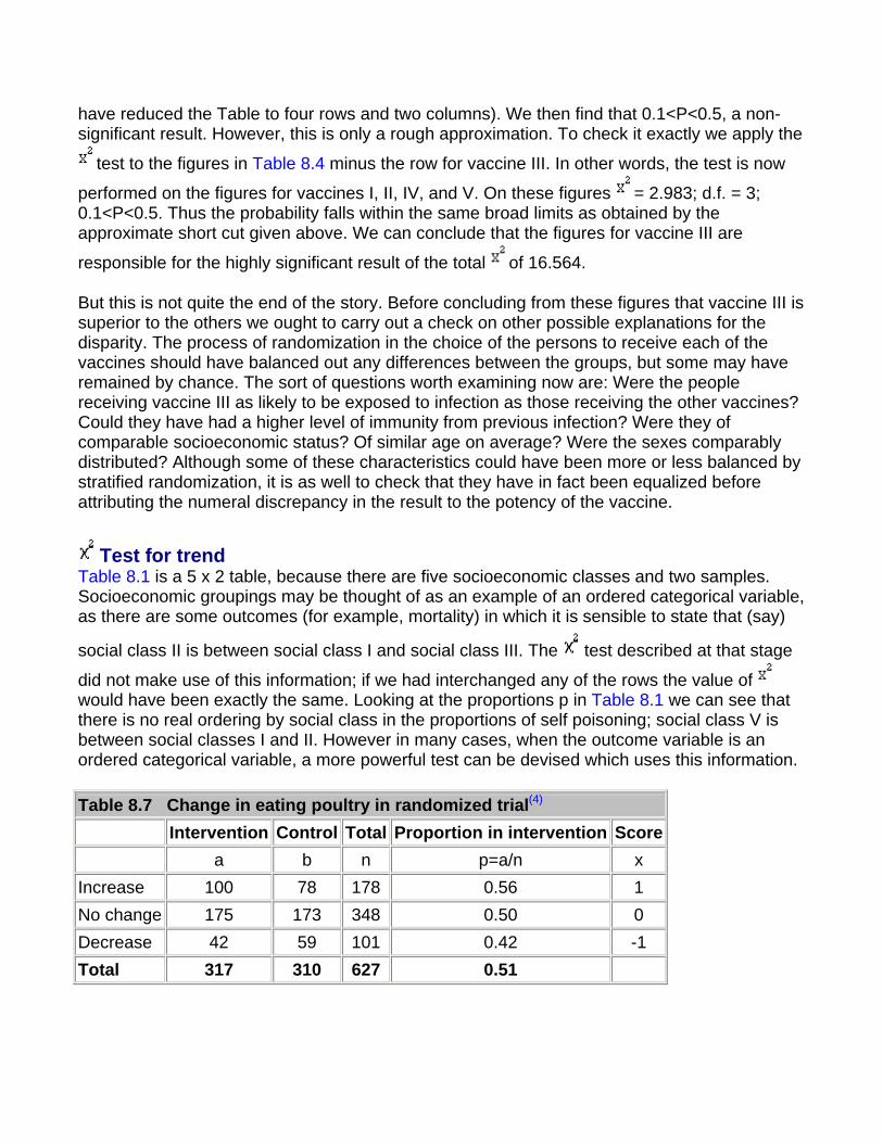
have reduced the Table to four rows and two columns). We then find that 0.1<P<0.5, a non-significant result. However, this is only a rough approximation. To check it exactly we apply the

test to the figures in Table 8.4 minus the row for vaccine III. In other words, the test is now

performed on the figures for vaccines I, II, IV, and V. On these figures = 2.983; d.f. = 3; 0.1<P<0.5. Thus the probability falls within the same broad limits as obtained by the approximate short cut given above. We can conclude that the figures for vaccine III are

responsible for the highly significant result of the total of 16.564.

But this is not quite the end of the story. Before concluding from these figures that vaccine III is superior to the others we ought to carry out a check on other possible explanations for the disparity. The process of randomization in the choice of the persons to receive each of the vaccines should have balanced out any differences between the groups, but some may have remained by chance. The sort of questions worth examining now are: Were the people receiving vaccine III as likely to be exposed to infection as those receiving the other vaccines? Could they have had a higher level of immunity from previous infection? Were they of comparable socioeconomic status? Of similar age on average? Were the sexes comparably distributed? Although some of these characteristics could have been more or less balanced by stratified randomization, it is as well to check that they have in fact been equalized before attributing the numeral discrepancy in the result to the potency of the vaccine.

Test for trend Table 8.1 is a 5 x 2 table, because there are five socioeconomic classes and two samples. Socioeconomic groupings may be thought of as an example of an ordered categorical variable, as there are some outcomes (for example, mortality) in which it is sensible to state that (say)

social class II is between social class I and social class III. The test described at that stage

did not make use of this information; if we had interchanged any of the rows the value of would have been exactly the same. Looking at the proportions p in Table 8.1 we can see that there is no real ordering by social class in the proportions of self poisoning; social class V is between social classes I and II. However in many cases, when the outcome variable is an ordered categorical variable, a more powerful test can be devised which uses this information.

Table 8.7 Change in eating poultry in randomized trial(4) Intervention Control Total Proportion in intervention Score

a b n p=a/n x Increase 100 78 178 0.56 1 No change 175 173 348 0.50 0 Decrease 42 59 101 0.42 -1 Total 317 310 627 0.51

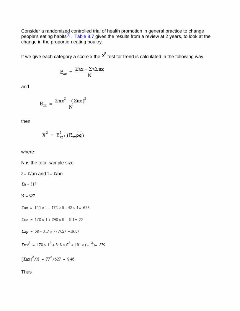
Consider a randomized controlled trial of health promotion in general practice to change people's eating habits(5). Table 8.7 gives the results from a review at 2 years, to look at the change in the proportion eating poultry.

If we give each category a score x the test for trend is calculated in the following way:

and

then

where:

N is the total sample size

= /an and = /bn

Thus

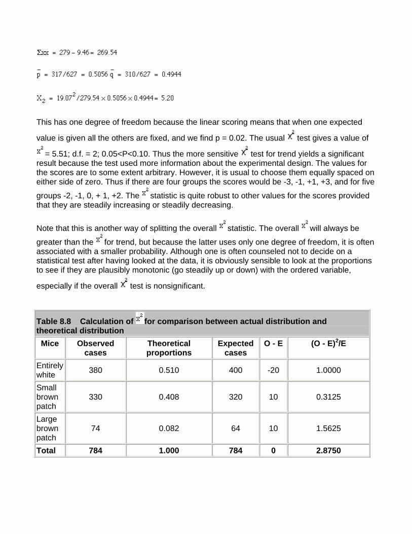
This has one degree of freedom because the linear scoring means that when one expected

value is given all the others are fixed, and we find p = 0.02. The usual test gives a value of

= 5.51; d.f. = 2; 0.05<P<0.10. Thus the more sensitive test for trend yields a significant result because the test used more information about the experimental design. The values for the scores are to some extent arbitrary. However, it is usual to choose them equally spaced on either side of zero. Thus if there are four groups the scores would be -3, -1, +1, +3, and for five

groups -2, -1, 0, + 1, +2. The statistic is quite robust to other values for the scores provided that they are steadily increasing or steadily decreasing.

Note that this is another way of splitting the overall statistic. The overall will always be

greater than the for trend, but because the latter uses only one degree of freedom, it is often associated with a smaller probability. Although one is often counseled not to decide on a statistical test after having looked at the data, it is obviously sensible to look at the proportions to see if they are plausibly monotonic (go steadily up or down) with the ordered variable,

especially if the overall test is nonsignificant.

Table 8.8 Calculation of for comparison between actual distribution and theoretical distribution Mice Observed

cases Theoretical proportions

Expected cases

O - E (O - E)2/E

Entirely white 380 0.510 400 -20 1.0000

Small brown patch

330 0.408 320 10 0.3125

Large brown patch

74 0.082 64 10 1.5625

Total 784 1.000 784 0 2.8750

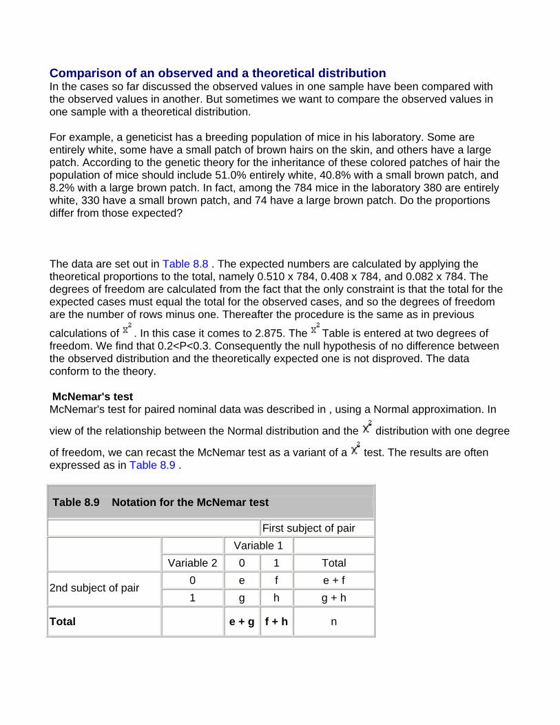
Comparison of an observed and a theoretical distribution In the cases so far discussed the observed values in one sample have been compared with the observed values in another. But sometimes we want to compare the observed values in one sample with a theoretical distribution.

For example, a geneticist has a breeding population of mice in his laboratory. Some are entirely white, some have a small patch of brown hairs on the skin, and others have a large patch. According to the genetic theory for the inheritance of these colored patches of hair the population of mice should include 51.0% entirely white, 40.8% with a small brown patch, and 8.2% with a large brown patch. In fact, among the 784 mice in the laboratory 380 are entirely white, 330 have a small brown patch, and 74 have a large brown patch. Do the proportions differ from those expected?

The data are set out in Table 8.8 . The expected numbers are calculated by applying the theoretical proportions to the total, namely 0.510 x 784, 0.408 x 784, and 0.082 x 784. The degrees of freedom are calculated from the fact that the only constraint is that the total for the expected cases must equal the total for the observed cases, and so the degrees of freedom are the number of rows minus one. Thereafter the procedure is the same as in previous

calculations of . In this case it comes to 2.875. The Table is entered at two degrees of freedom. We find that 0.2<P<0.3. Consequently the null hypothesis of no difference between the observed distribution and the theoretically expected one is not disproved. The data conform to the theory.

McNemar's test McNemar's test for paired nominal data was described in , using a Normal approximation. In

view of the relationship between the Normal distribution and the distribution with one degree

of freedom, we can recast the McNemar test as a variant of a test. The results are often expressed as in Table 8.9 .

Table 8.9 Notation for the McNemar test

First subject of pair Variable 1

Variable 2 0 1 Total

0 e f e + f 2nd subject of pair

1 g h g + h

Total e + g f + h n

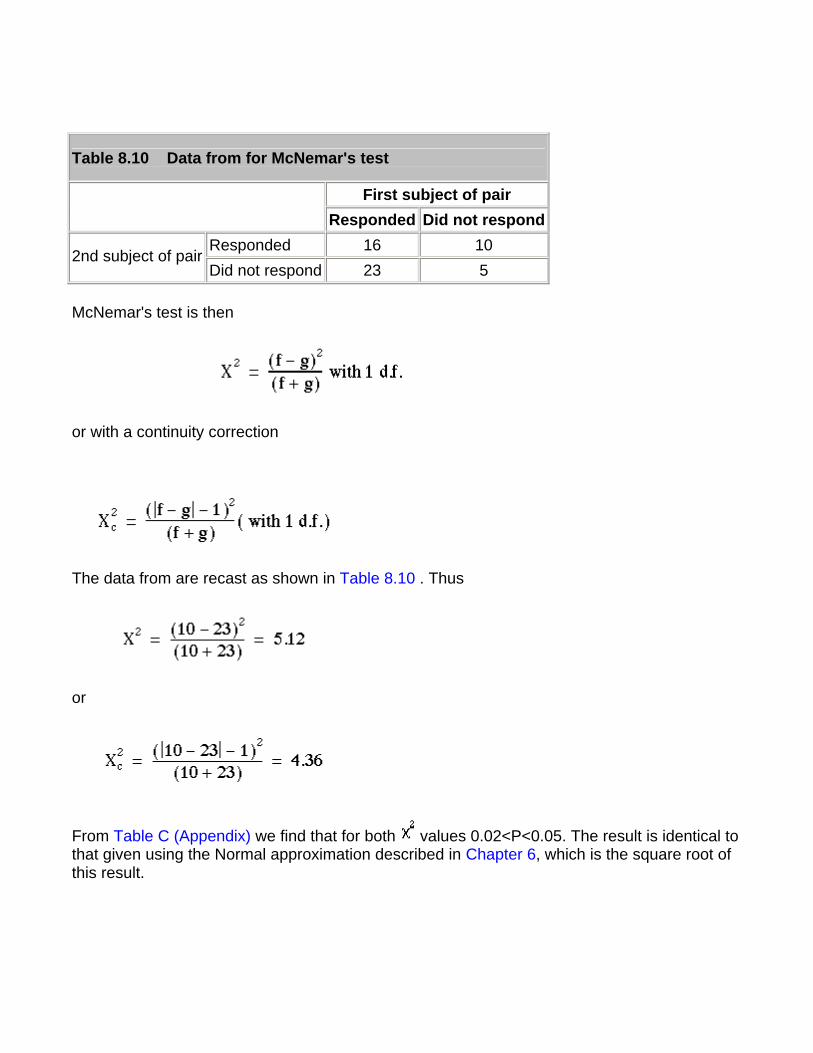
Table 8.10 Data from for McNemar's test

First subject of pair Responded Did not respond

Responded 16 10 2nd subject of pair

Did not respond 23 5

McNemar's test is then

or with a continuity correction

The data from are recast as shown in Table 8.10 . Thus

or

From Table C (Appendix) we find that for both values 0.02<P<0.05. The result is identical to that given using the Normal approximation described in Chapter 6, which is the square root of this result.

Extensions of the test

If the outcome variable in a study is nominal, the test can be extended to look at the effect of more than one input variable, for example to allow for confounding variables. This is most easily done using multiple logistic regression , a generalization of multiple regression , which is described in Chapter 11. If the data are matched, then a further technique ( conditional logistic regression ) should be employed. This is described in advanced textbooks and will not be discussed further here.

Common questions

I have matched data, but the matching criteria were very weak. Should I use McNemar's test? The general principle is that if the data are matched in any way, the analysis should take account of it. If the matching is weak then the matched analysis and the unmatched analysis should agree. In some cases when there are a large number of pairs with the same outcome, it would appear that the McNemar's test is discarding a lot of information, and so is losing power. However, imagine we are trying to decide which of two high jumpers is the better. They each jump over a bar at a fixed height, and then the height is increased. It is only when one fails to jump a given height and the other succeeds that a winner can be announced. It does not matter how many jumps both have cleared.

References

1. Snedecor GW, Cochran WG. In: Statistical Methods , 7th ed. Iowa: Iowa State University Press, 191,0:47.

2. Cochran WG. Some methods for strengthening the common tests. Biometrics 1956; l0 :4l7-5l.

3. Yates F. Contingency tables involving small numbers and the test. J Roy Stat Soc Suppl 1934; 1:217-3. 4. Capples ME, McKnight A. Randomized controlled trial of health promotions in general practice for patients at high cardiovascular risk. BMJ l994;3O9:993-6.

Exercises

Exercise 8.1 In a trial of new drug against a standard drug for the treatment of depression the new drug caused some improvement in 56% of 73 patients and the standard drug some improvement in 41% of 70 patients. The results were assessed in five categories as follows:

New treatment: much improved 18, improved 23, unchanged 15, worse 9, much worse 8;

Standard treatment: much improved 12, improved 17, unchanged 19, worse 13, much worse 9.

What is the value of which takes no account of the ordered value of data, what is the value

of the test for trend, and the P value? How many degrees of freedom are there? What is the value of P in each case?

Exercise 8.2 An outbreak of pediculosis capitis is being investigated in a girls' school containing 291 pupils. Of 130 children who live in a nearby housing estate 18 were infested

and of 161 who live elsewhere 37 were infested. What is the value of the difference, and what is its significance? Find the difference in infestation rates and a 95% confidence interval for the difference.

Exercise 8.3 The 55 affected girls were divided at random into two groups of 29 and 26. The first group received a standard local application and the second group a new local application. The efficacy of each was measured by clearance of the infestation after one application. By this measure the standard application failed in ten cases and the new

application in five. What is the value of the difference (with Yates' correction), and what is its significance? What is the difference in clearance rates and an approximate 95% confidence interval?

Exercise 8.4 A general practitioner reviewed all patient notes in four practices for 1 year. Newly diagnosed cases of asthma were noted, and whether or not the case was referred to hospital. The following referrals were found (total cases in parentheses): practice A, 14 (103);

practice B, 11 (92); practice C, 39 (166); practice D, 31 (221). What are the and P values for the distribution of the referrals in these practices? Do they suggest that any one practice has significantly more referrals than others?

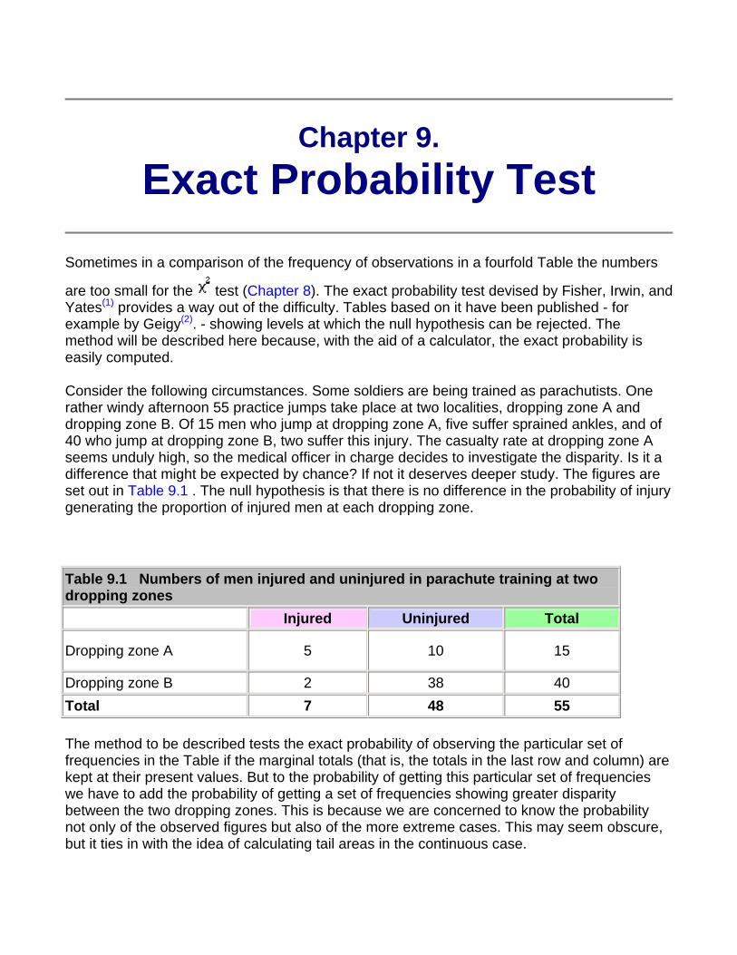
Chapter 9. Exact Probability Test

Sometimes in a comparison of the frequency of observations in a fourfold Table the numbers

are too small for the test (Chapter 8). The exact probability test devised by Fisher, Irwin, and Yates(1) provides a way out of the difficulty. Tables based on it have been published - for example by Geigy(2). - showing levels at which the null hypothesis can be rejected. The method will be described here because, with the aid of a calculator, the exact probability is easily computed.

Consider the following circumstances. Some soldiers are being trained as parachutists. One rather windy afternoon 55 practice jumps take place at two localities, dropping zone A and dropping zone B. Of 15 men who jump at dropping zone A, five suffer sprained ankles, and of 40 who jump at dropping zone B, two suffer this injury. The casualty rate at dropping zone A seems unduly high, so the medical officer in charge decides to investigate the disparity. Is it a difference that might be expected by chance? If not it deserves deeper study. The figures are set out in Table 9.1 . The null hypothesis is that there is no difference in the probability of injury generating the proportion of injured men at each dropping zone.

Table 9.1 Numbers of men injured and uninjured in parachute training at two dropping zones

Injured Uninjured Total

Dropping zone A 5 10 15

Dropping zone B 2 38 40 Total 7 48 55

The method to be described tests the exact probability of observing the particular set of frequencies in the Table if the marginal totals (that is, the totals in the last row and column) are kept at their present values. But to the probability of getting this particular set of frequencies we have to add the probability of getting a set of frequencies showing greater disparity between the two dropping zones. This is because we are concerned to know the probability not only of the observed figures but also of the more extreme cases. This may seem obscure, but it ties in with the idea of calculating tail areas in the continuous case.

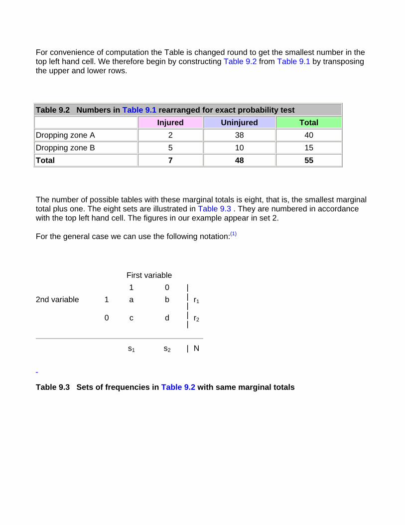
For convenience of computation the Table is changed round to get the smallest number in the top left hand cell. We therefore begin by constructing Table 9.2 from Table 9.1 by transposing the upper and lower rows.

Table 9.2 Numbers in Table 9.1 rearranged for exact probability test Injured Uninjured Total

Dropping zone A 2 38 40 Dropping zone B 5 10 15 Total 7 48 55

The number of possible tables with these marginal totals is eight, that is, the smallest marginal total plus one. The eight sets are illustrated in Table 9.3 . They are numbered in accordance with the top left hand cell. The figures in our example appear in set 2.

For the general case we can use the following notation:(1)

First variable 1 0 2nd variable 1 a b r1

0 c d

|||||

r2

s1 s2 | N

Table 9.3 Sets of frequencies in Table 9.2 with same marginal totals

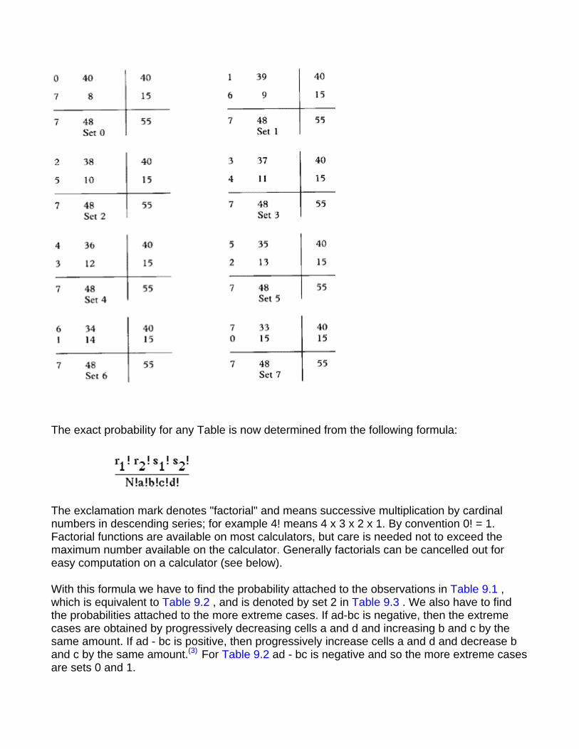
The exact probability for any Table is now determined from the following formula:

The exclamation mark denotes "factorial" and means successive multiplication by cardinal numbers in descending series; for example 4! means 4 x 3 x 2 x 1. By convention 0! = 1. Factorial functions are available on most calculators, but care is needed not to exceed the maximum number available on the calculator. Generally factorials can be cancelled out for easy computation on a calculator (see below).

With this formula we have to find the probability attached to the observations in Table 9.1 , which is equivalent to Table 9.2 , and is denoted by set 2 in Table 9.3 . We also have to find the probabilities attached to the more extreme cases. If ad-bc is negative, then the extreme cases are obtained by progressively decreasing cells a and d and increasing b and c by the same amount. If ad - bc is positive, then progressively increase cells a and d and decrease b and c by the same amount.(3) For Table 9.2 ad - bc is negative and so the more extreme cases are sets 0 and 1.

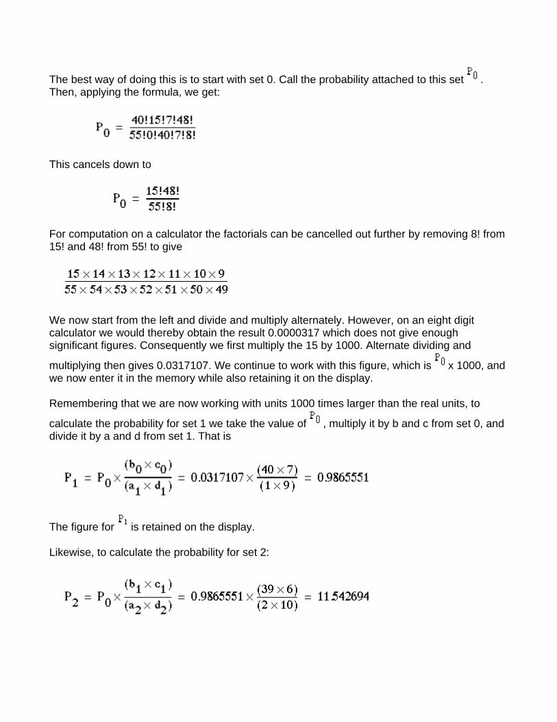
The best way of doing this is to start with set 0. Call the probability attached to this set . Then, applying the formula, we get:

This cancels down to

For computation on a calculator the factorials can be cancelled out further by removing 8! from 15! and 48! from 55! to give

We now start from the left and divide and multiply alternately. However, on an eight digit calculator we would thereby obtain the result 0.0000317 which does not give enough significant figures. Consequently we first multiply the 15 by 1000. Alternate dividing and

multiplying then gives 0.0317107. We continue to work with this figure, which is x 1000, and we now enter it in the memory while also retaining it on the display.

Remembering that we are now working with units 1000 times larger than the real units, to

calculate the probability for set 1 we take the value of , multiply it by b and c from set 0, and divide it by a and d from set 1. That is

The figure for is retained on the display.

Likewise, to calculate the probability for set 2:

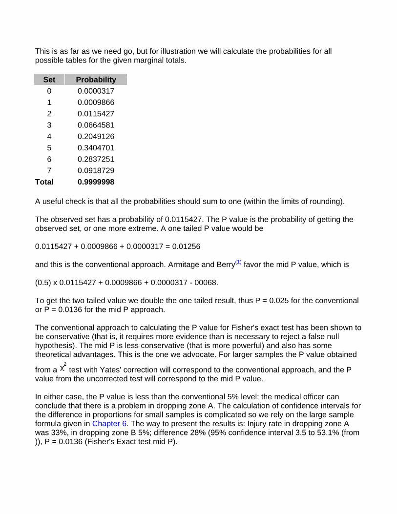
This is as far as we need go, but for illustration we will calculate the probabilities for all possible tables for the given marginal totals.

Set Probability 0 0.0000317 1 0.0009866 2 0.0115427 3 0.0664581 4 0.2049126 5 0.3404701 6 0.2837251 7 0.0918729

Total 0.9999998

A useful check is that all the probabilities should sum to one (within the limits of rounding).

The observed set has a probability of 0.0115427. The P value is the probability of getting the observed set, or one more extreme. A one tailed P value would be

0.0115427 + 0.0009866 + 0.0000317 = 0.01256

and this is the conventional approach. Armitage and Berry(1) favor the mid P value, which is

(0.5) x 0.0115427 + 0.0009866 + 0.0000317 - 00068.

To get the two tailed value we double the one tailed result, thus P = 0.025 for the conventional or P = 0.0136 for the mid P approach.

The conventional approach to calculating the P value for Fisher's exact test has been shown to be conservative (that is, it requires more evidence than is necessary to reject a false null hypothesis). The mid P is less conservative (that is more powerful) and also has some theoretical advantages. This is the one we advocate. For larger samples the P value obtained

from a test with Yates' correction will correspond to the conventional approach, and the P value from the uncorrected test will correspond to the mid P value.

In either case, the P value is less than the conventional 5% level; the medical officer can conclude that there is a problem in dropping zone A. The calculation of confidence intervals for the difference in proportions for small samples is complicated so we rely on the large sample formula given in Chapter 6. The way to present the results is: Injury rate in dropping zone A was 33%, in dropping zone B 5%; difference 28% (95% confidence interval 3.5 to 53.1% (from )), P = 0.0136 (Fisher's Exact test mid P).

Common questions

Why is Fisher's test called an exact test? Because of the discrete nature of the data, and the limited amount of it, combinations of results which give the same marginal totals can be listed, and probabilities attached to them. Thus, given these marginal totals we can work out exactly what is the probability of getting an observed result, in the same way that we can work out exactly the probability of getting six heads out of ten tosses of a fair coin. One difficulty is that there may not be combinations which correspond "exactly" to 95%, 50 we cannot get an "exact" 95% confidence interval but (say) one with a 97% coverage or one with a 94% coverage.

References 1. Armitage P, Berry G. In: Statistical Methods in Medical Research. Oxford: Blackwell Scientific Publications, 1994:1234. 2. Lentner C, ed. Geige Scientific Tables, 8th ed. Basle: Geigy, 1982. 3. Strike PW. Statistical Methods in Laboratory Medicine. Oxford: Butterworth-Heinemann, 1991.

Exercises

Exercise 9.1 Of 30 men employed in a small workshop 18 worked in one department and 12 in another department. In one year five of the 18 reported sick with septic hands, and of the 12 men in the other department one did so. Is there a difference in the departments and how would you report this result?

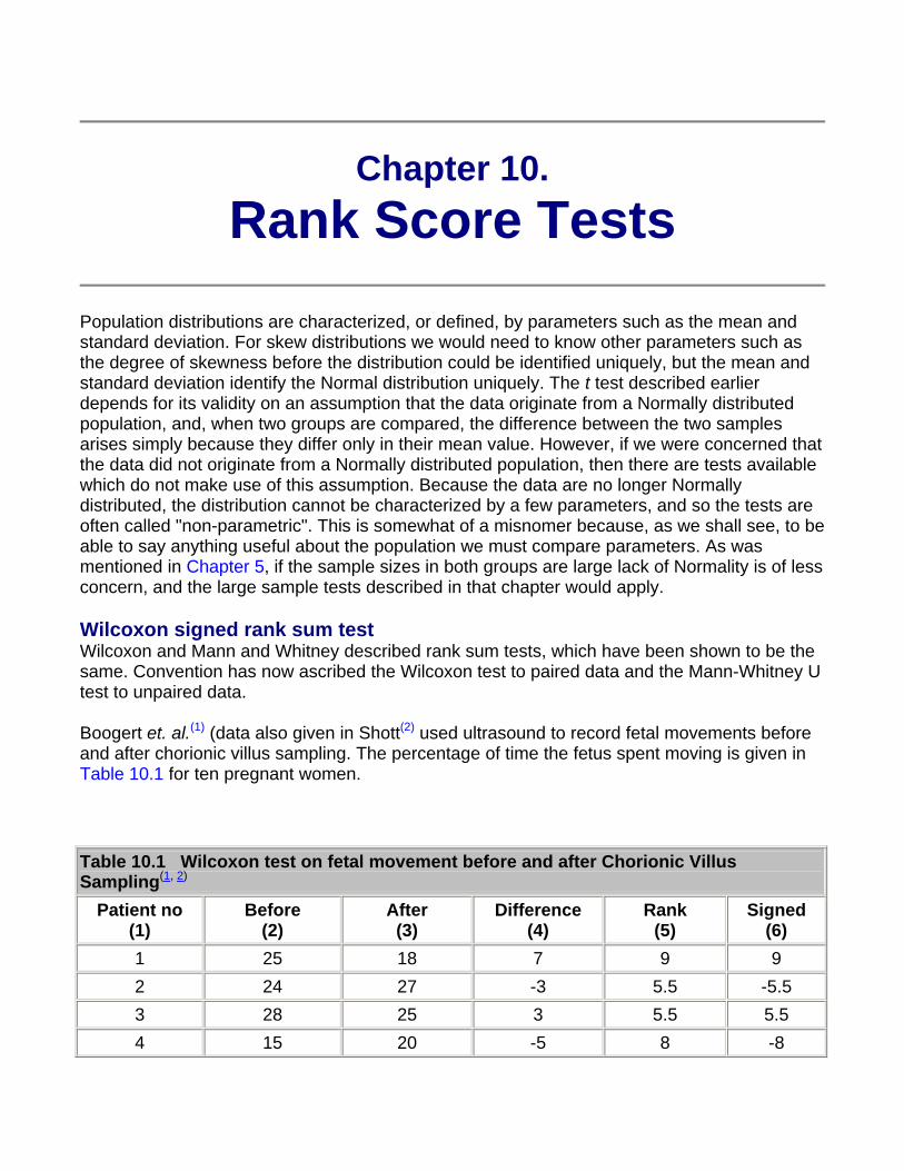
Chapter 10. Rank Score Tests

Population distributions are characterized, or defined, by parameters such as the mean and standard deviation. For skew distributions we would need to know other parameters such as the degree of skewness before the distribution could be identified uniquely, but the mean and standard deviation identify the Normal distribution uniquely. The t test described earlier depends for its validity on an assumption that the data originate from a Normally distributed population, and, when two groups are compared, the difference between the two samples arises simply because they differ only in their mean value. However, if we were concerned that the data did not originate from a Normally distributed population, then there are tests available which do not make use of this assumption. Because the data are no longer Normally distributed, the distribution cannot be characterized by a few parameters, and so the tests are often called "non-parametric". This is somewhat of a misnomer because, as we shall see, to be able to say anything useful about the population we must compare parameters. As was mentioned in Chapter 5, if the sample sizes in both groups are large lack of Normality is of less concern, and the large sample tests described in that chapter would apply.

Wilcoxon signed rank sum test Wilcoxon and Mann and Whitney described rank sum tests, which have been shown to be the same. Convention has now ascribed the Wilcoxon test to paired data and the Mann-Whitney U test to unpaired data.

Boogert et. al.(1) (data also given in Shott(2) used ultrasound to record fetal movements before and after chorionic villus sampling. The percentage of time the fetus spent moving is given in Table 10.1 for ten pregnant women.

Table 10.1 Wilcoxon test on fetal movement before and after Chorionic Villus Sampling(1, 2)

Patient no (1)

Before (2)

After (3)

Difference (4)

Rank (5)

Signed (6)

1 25 18 7 9 9 2 24 27 -3 5.5 -5.5 3 28 25 3 5.5 5.5 4 15 20 -5 8 -8

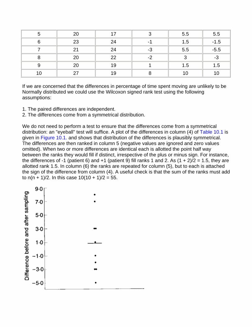
5 20 17 3 5.5 5.5 6 23 24 -1 1.5 -1.5 7 21 24 -3 5.5 -5.5 8 20 22 -2 3 -3 9 20 19 1 1.5 1.5

10 27 19 8 10 10

If we are concerned that the differences in percentage of time spent moving are unlikely to be Normally distributed we could use the Wilcoxon signed rank test using the following assumptions:

1. The paired differences are independent. 2. The differences come from a symmetrical distribution.

We do not need to perform a test to ensure that the differences come from a symmetrical distribution: an "eyeball" test will suffice. A plot of the differences in column (4) of Table 10.1 is given in Figure 10.1. and shows that distribution of the differences is plausibly symmetrical. The differences are then ranked in column 5 (negative values are ignored and zero values omitted). When two or more differences are identical each is allotted the point half way between the ranks they would fill if distinct, irrespective of the plus or minus sign. For instance, the differences of -1 (patient 6) and +1 (patient 9) fill ranks 1 and 2. As (1 + 2)/2 = 1.5, they are allotted rank 1.5. In column (6) the ranks are repeated for column (5), but to each is attached the sign of the difference from column (4). A useful check is that the sum of the ranks must add to n(n + 1)/2. In this case 10(10 + 1)/2 = 55.

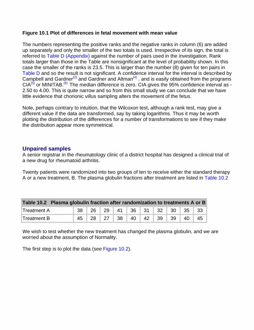
Figure 10.1 Plot of differences in fetal movement with mean value

The numbers representing the positive ranks and the negative ranks in column (6) are added up separately and only the smaller of the two totals is used. Irrespective of its sign, the total is referred to Table D (Appendix) against the number of pairs used in the investigation. Rank totals larger than those in the Table are nonsignificant at the level of probability shown. In this case the smaller of the ranks is 23.5. This is larger than the number (8) given for ten pairs in Table D and so the result is not significant. A confidence interval for the interval is described by Campbell and Gardner(2) and Gardner and Altman(4) . and is easily obtained from the programs CIA(5) or MINITAB.(6) The median difference is zero. CIA gives the 95% confidence interval as - 2.50 to 4.00. This is quite narrow and so from this small study we can conclude that we have little evidence that chorionic villus sampling alters the movement of the fetus.

Note, perhaps contrary to intuition, that the Wilcoxon test, although a rank test, may give a different value if the data are transformed, say by taking logarithms. Thus it may be worth plotting the distribution of the differences for a number of transformations to see if they make the distribution appear more symmetrical.

Unpaired samples A senior registrar in the rheumatology clinic of a district hospital has designed a clinical trial of a new drug for rheumatoid arthritis.

Twenty patients were randomized into two groups of ten to receive either the standard therapy A or a new treatment, B. The plasma globulin fractions after treatment are listed in Table 10.2

Table 10.2 Plasma globulin fraction after randomization to treatments A or BTreatment A 38 26 29 41 36 31 32 30 35 33 Treatment B 45 28 27 38 40 42 39 39 40 45

We wish to test whether the new treatment has changed the plasma globulin, and we are worried about the assumption of Normality.

The first step is to plot the data (see Figure 10.2).

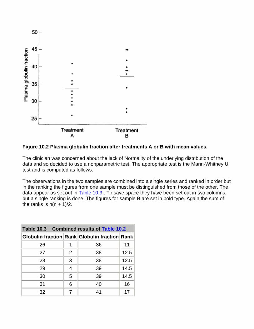
Figure 10.2 Plasma globulin fraction after treatments A or B with mean values.

The clinician was concerned about the lack of Normality of the underlying distribution of the data and so decided to use a nonparametric test. The appropriate test is the Mann-Whitney U test and is computed as follows.

The observations in the two samples are combined into a single series and ranked in order but in the ranking the figures from one sample must be distinguished from those of the other. The data appear as set out in Table 10.3 . To save space they have been set out in two columns, but a single ranking is done. The figures for sample B are set in bold type. Again the sum of the ranks is n(n + 1)/2.

Table 10.3 Combined results of Table 10.2 Globulin fraction Rank Globulin fraction Rank

26 1 36 11 27 2 38 12.528 3 38 12.529 4 39 14.530 5 39 14.531 6 40 16 32 7 41 17

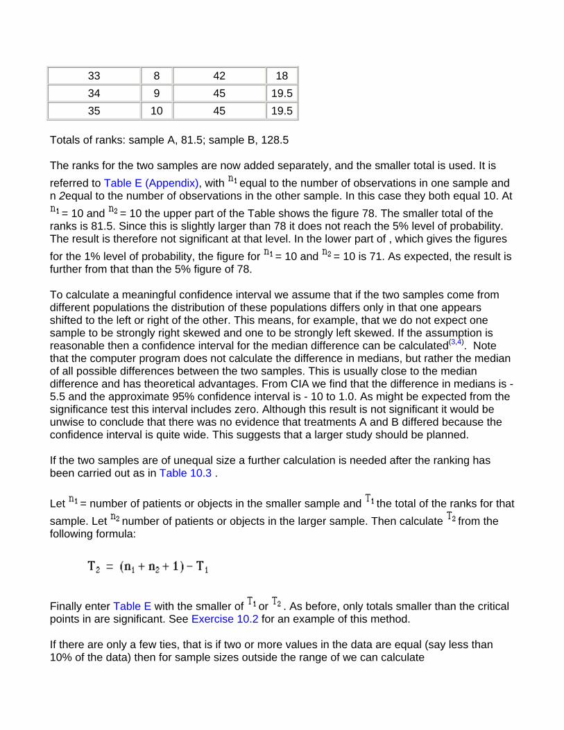
33 8 42 18 34 9 45 19.535 10 45 19.5

Totals of ranks: sample A, 81.5; sample B, 128.5

The ranks for the two samples are now added separately, and the smaller total is used. It is referred to Table E (Appendix), with equal to the number of observations in one sample and n 2equal to the number of observations in the other sample. In this case they both equal 10. At

= 10 and = 10 the upper part of the Table shows the figure 78. The smaller total of the ranks is 81.5. Since this is slightly larger than 78 it does not reach the 5% level of probability. The result is therefore not significant at that level. In the lower part of , which gives the figures for the 1% level of probability, the figure for = 10 and = 10 is 71. As expected, the result is further from that than the 5% figure of 78.

To calculate a meaningful confidence interval we assume that if the two samples come from different populations the distribution of these populations differs only in that one appears shifted to the left or right of the other. This means, for example, that we do not expect one sample to be strongly right skewed and one to be strongly left skewed. If the assumption is reasonable then a confidence interval for the median difference can be calculated(3,4). Note that the computer program does not calculate the difference in medians, but rather the median of all possible differences between the two samples. This is usually close to the median difference and has theoretical advantages. From CIA we find that the difference in medians is -5.5 and the approximate 95% confidence interval is - 10 to 1.0. As might be expected from the significance test this interval includes zero. Although this result is not significant it would be unwise to conclude that there was no evidence that treatments A and B differed because the confidence interval is quite wide. This suggests that a larger study should be planned.

If the two samples are of unequal size a further calculation is needed after the ranking has been carried out as in Table 10.3 .

Let = number of patients or objects in the smaller sample and the total of the ranks for that sample. Let number of patients or objects in the larger sample. Then calculate from the following formula:

Finally enter Table E with the smaller of or . As before, only totals smaller than the critical points in are significant. See Exercise 10.2 for an example of this method.

If there are only a few ties, that is if two or more values in the data are equal (say less than 10% of the data) then for sample sizes outside the range of we can calculate

On the null hypothesis that the two samples come from the same population, z is approximately Normally distributed, mean zero and standard deviation one, and can be referred to Table A (Appendix) to calculate the P value.

From the data of Table 10.2 we obtain

and from Table A we find that P is about 0.075, which corroborates the earlier result.

The advantages of these tests based on ranking are that they can be safely used on data that are not at all Normally distributed, that they are quick to carry out, and that no calculator is needed. Non-Normally distributed data can sometimes be transformed by the use of logarithms or some other method to make them Normally distributed, and a t test performed. Consequently the best procedure to adopt may require careful thought. The extent and nature of the difference between two samples is often brought out more clearly by standard deviations and t tests than by non-parametric tests.

Common questions

Non-parametric tests are valid for both non-Normally distributed data and Normally distributed data, so why not use them all the time? It would seem prudent to use non-parametric tests in all cases, which would save one the bother of testing for Normality. Parametric tests are preferred, however, for the following reasons:

1. As I have tried to emphasize in this book, we are rarely interested in a significance test alone; we would like to say something about the population from which the samples came, and this is best done with estimates of parameters and confidence intervals. 2. It is difficult to do flexible modeling with non-parametric tests, for example allowing for confounding factors using multiple regression (see Chapter 11).

Do non-parametric tests compare medians? It is a commonly held belief that a Mann-Whitney U test is in fact a test for differences in

medians. However, two groups could have the same median and yet have a significant Mann-Whitney U test. Consider the following data for two groups, each with 100 observations. Group 1: 98 (0), 1, 2; Group 2: 51 (0), 1, 48 (2). The median in both cases is 0, but from the Mann-Whitney test P<0.000 1.

Only if we are prepared to make the additional assumption that the difference in the two groups is simply a shift in location (that is, the distribution of the data in one group is simply shifted by a fixed amount from the other) can we say that the test is a test of the difference in medians. However, if the groups have the same distribution, then a shift in location will move medians and means by the same amount and so the difference in medians is the same as the difference in means. Thus the Mann-Whitney U test is also a test for the difference in means.

How is the Mann- Whitney U test related to the t test? If one were to input the ranks of the data rather than the data themselves into a two sample t test program, the P value obtained would be very close to that produced by a Mann-Whitney U test.

References

1. Boogert A, Manhigh A, Visser GHA. The immediate effects of chronic villus sampling on fetal movements. Am J Obstet Gynecol 1987; 157 :137-9.

2. Shott S. Statistics for Health Professionals. Philadelphia: WB Saunders, 1990. 3. Campbell MJ, Gardner MJ. Calculating confidence intervals for some non-parametric analyses. BMJ l988;

296 :l369-7l. 4. Gardner MJ, Altman DG. Statistics with Confidence . Confidence Intervals and Statistical Guidelines.

London: BMJ Publishing Group, 1989. 5. Gardner MJ, Gardner SB, Winter PD. CIA (Confidence Interval Analysis) . London: BMJ Publishing

Group, 1989. 6. Ryan BF, Joiner BL, Ryan TA. Minitab Handbook , 2nd ed. Boston: Duxbury Press, 1985.

Exercises

Exercise 10.1 A new treatment in the form of tablets for the prophylaxis of migraine has been introduced, to be taken before an impending attack. Twelve patients agree to try this remedy in addition to the usual general measures they take, subject to advice from their doctor on the taking of analgesics also.

A crossover trial with identical placebo tablets is carried out over a period of 8 months. The numbers of attacks experienced by each patient on, first, the new treatment and, secondly, the placebo were as follows: patient (1) 4 and 2; patient (2) 12 and 6; patient (3) 6 and 6; patient (4) 3 and 5; patient (5)15 and 9; patient (6) 10 and 11; patient (7) 2 and 4; patient (8) 5 and 6; patient (9)11 and 3; patient (10) 4 and 7; patient (11) 6 and 0; patient (12) 2 and 5. In a Wilcoxon rank sum test what is the smaller total of ranks? Is it significant at the 5% level?

Exercise 10.2 Another doctor carried out a similar pilot study with this preparation on 12 patients, giving the same placebo to ten other patients. The numbers of migraine attacks experienced by the patients over a period of 6 months were as follows.

Group receiving new preparation: patient (1) 8; (2) 6; (3) 0; (4) 3; (5) 14; (6) 5; (7) 11; (8) 2

Group receiving placebo: patient (9) 7; (10) 10; (11) 4; (12) 11; (13) 2; (14) 8; (15) 8; (16) 6; (17)1; (18) 5.

In a Mann-Whitney two sample test what is the smaller total of ranks? Which sample of patients provides it? Is the difference significant at the 5% level?

Chapter 11. Correlation and Regression

The word correlation is used in everyday life to denote some form of association. We might say that we have noticed a correlation between foggy days and attacks of wheezing. However, in statistical terms we use correlation to denote association between two quantitative variables. We also assume that the association is linear, that one variable increases or decreases a fixed amount for a unit increase or decrease in the other. The other technique that is often used in these circumstances is regression, which involves estimating the best straight line to summarize the association.

Correlation coefficient The degree of association is measured by a correlation coefficient, denoted by r. It is sometimes called Pearson's correlation coefficient after its originator and is a measure of linear association. If a curved line is needed to express the relationship, other and more complicated measures of the correlation must be used.

The correlation coefficient is measured on a scale that varies from + 1 through 0 to - 1. Complete correlation between two variables is expressed by either + 1 or -1. When one variable increases as the other increases the correlation is positive; when one decreases as the other increases it is negative. Complete absence of correlation is represented by 0. Figure 11.1 gives some graphical representations of correlation.

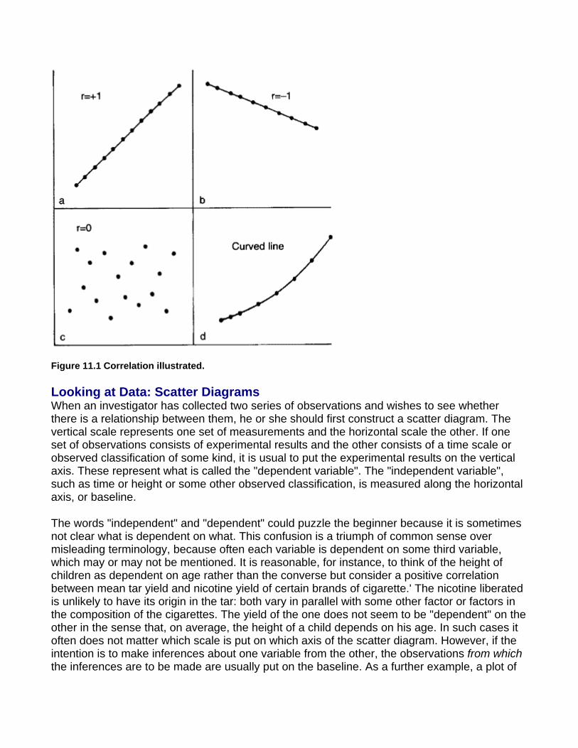
Figure 11.1 Correlation illustrated.

Looking at Data: Scatter Diagrams When an investigator has collected two series of observations and wishes to see whether there is a relationship between them, he or she should first construct a scatter diagram. The vertical scale represents one set of measurements and the horizontal scale the other. If one set of observations consists of experimental results and the other consists of a time scale or observed classification of some kind, it is usual to put the experimental results on the vertical axis. These represent what is called the "dependent variable". The "independent variable", such as time or height or some other observed classification, is measured along the horizontal axis, or baseline.

The words "independent" and "dependent" could puzzle the beginner because it is sometimes not clear what is dependent on what. This confusion is a triumph of common sense over misleading terminology, because often each variable is dependent on some third variable, which may or may not be mentioned. It is reasonable, for instance, to think of the height of children as dependent on age rather than the converse but consider a positive correlation between mean tar yield and nicotine yield of certain brands of cigarette.' The nicotine liberated is unlikely to have its origin in the tar: both vary in parallel with some other factor or factors in the composition of the cigarettes. The yield of the one does not seem to be "dependent" on the other in the sense that, on average, the height of a child depends on his age. In such cases it often does not matter which scale is put on which axis of the scatter diagram. However, if the intention is to make inferences about one variable from the other, the observations from which the inferences are to be made are usually put on the baseline. As a further example, a plot of

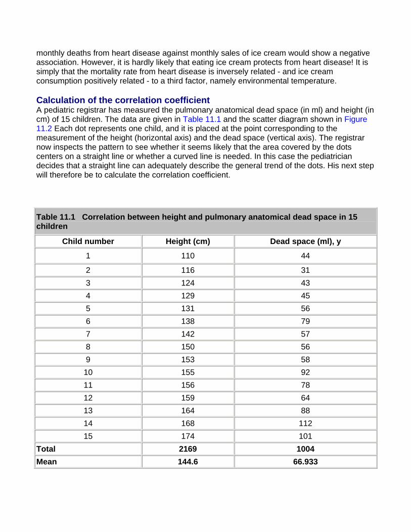
monthly deaths from heart disease against monthly sales of ice cream would show a negative association. However, it is hardly likely that eating ice cream protects from heart disease! It is simply that the mortality rate from heart disease is inversely related - and ice cream consumption positively related - to a third factor, namely environmental temperature.

Calculation of the correlation coefficient A pediatric registrar has measured the pulmonary anatomical dead space (in ml) and height (in cm) of 15 children. The data are given in Table 11.1 and the scatter diagram shown in Figure 11.2 Each dot represents one child, and it is placed at the point corresponding to the measurement of the height (horizontal axis) and the dead space (vertical axis). The registrar now inspects the pattern to see whether it seems likely that the area covered by the dots centers on a straight line or whether a curved line is needed. In this case the pediatrician decides that a straight line can adequately describe the general trend of the dots. His next step will therefore be to calculate the correlation coefficient.

Table 11.1 Correlation between height and pulmonary anatomical dead space in 15 children

Child number Height (cm) Dead space (ml), y

1 110 44

2 116 31 3 124 43 4 129 45 5 131 56 6 138 79 7 142 57 8 150 56 9 153 58 10 155 92 11 156 78 12 159 64 13 164 88 14 168 112 15 174 101

Total 2169 1004 Mean 144.6 66.933

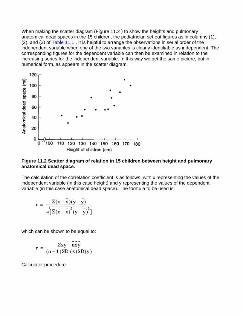
When making the scatter diagram (Figure 11.2 ) to show the heights and pulmonary anatomical dead spaces in the 15 children, the pediatrician set out figures as in columns (1), (2), and (3) of Table 11.1 . It is helpful to arrange the observations in serial order of the independent variable when one of the two variables is clearly identifiable as independent. The corresponding figures for the dependent variable can then be examined in relation to the increasing series for the independent variable. In this way we get the same picture, but in numerical form, as appears in the scatter diagram.

Figure 11.2 Scatter diagram of relation in 15 children between height and pulmonary anatomical dead space.

The calculation of the correlation coefficient is as follows, with x representing the values of the independent variable (in this case height) and y representing the values of the dependent variable (in this case anatomical dead space). The formula to be used is:

which can be shown to be equal to:

Calculator procedure

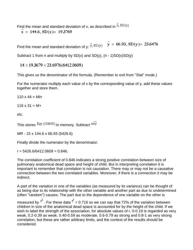
Find the mean and standard deviation of x, as described in

Find the mean and standard deviation of y:

Subtract 1 from n and multiply by SD(x) and SD(y), (n - 1)SD(x)SD(y)

This gives us the denominator of the formula. (Remember to exit from "Stat" mode.)

For the numerator multiply each value of x by the corresponding value of y, add these values together and store them.

110 x 44 = Min

116 x 31 = M+

etc.

This stores in memory. Subtract

MR - 15 x 144.6 x 66.93 (5426.6)

Finally divide the numerator by the denominator.

r = 5426.6/6412.0609 = 0.846.

The correlation coefficient of 0.846 indicates a strong positive correlation between size of pulmonary anatomical dead space and height of child. But in interpreting correlation it is important to remember that correlation is not causation. There may or may not be a causative connection between the two correlated variables. Moreover, if there is a connection it may be indirect.

A part of the variation in one of the variables (as measured by its variance) can be thought of as being due to its relationship with the other variable and another part as due to undetermined (often "random") causes. The part due to the dependence of one variable on the other is

measured by . For these data = 0.716 so we can say that 72% of the variation between children in size of the anatomical dead space is accounted for by the height of the child. If we wish to label the strength of the association, for absolute values of r, 0-0.19 is regarded as very weak, 0.2-0.39 as weak, 0.40-0.59 as moderate, 0.6-0.79 as strong and 0.8-1 as very strong correlation, but these are rather arbitrary limits, and the context of the results should be considered.

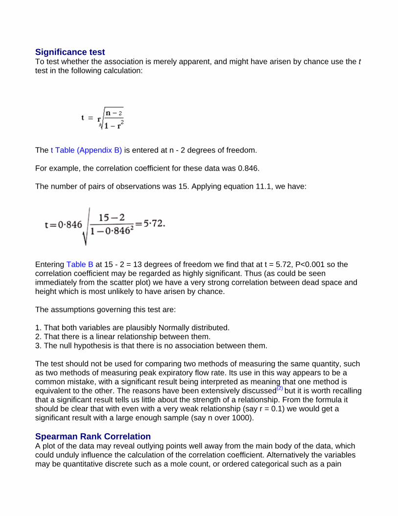
Significance test To test whether the association is merely apparent, and might have arisen by chance use the t test in the following calculation:

The t Table (Appendix B) is entered at n - 2 degrees of freedom.

For example, the correlation coefficient for these data was 0.846.

The number of pairs of observations was 15. Applying equation 11.1, we have:

Entering Table B at 15 - 2 = 13 degrees of freedom we find that at t = 5.72, P<0.001 so the correlation coefficient may be regarded as highly significant. Thus (as could be seen immediately from the scatter plot) we have a very strong correlation between dead space and height which is most unlikely to have arisen by chance.

The assumptions governing this test are:

1. That both variables are plausibly Normally distributed. 2. That there is a linear relationship between them. 3. The null hypothesis is that there is no association between them.

The test should not be used for comparing two methods of measuring the same quantity, such as two methods of measuring peak expiratory flow rate. Its use in this way appears to be a common mistake, with a significant result being interpreted as meaning that one method is equivalent to the other. The reasons have been extensively discussed(2) but it is worth recalling that a significant result tells us little about the strength of a relationship. From the formula it should be clear that with even with a very weak relationship (say r = 0.1) we would get a significant result with a large enough sample (say n over 1000).

Spearman Rank Correlation A plot of the data may reveal outlying points well away from the main body of the data, which could unduly influence the calculation of the correlation coefficient. Alternatively the variables may be quantitative discrete such as a mole count, or ordered categorical such as a pain

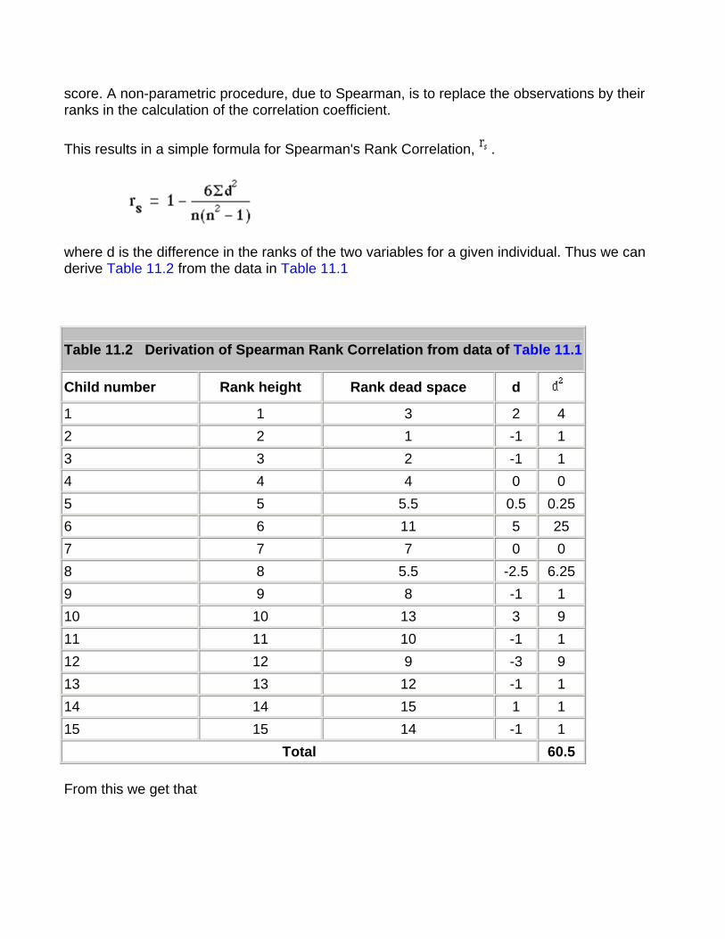
score. A non-parametric procedure, due to Spearman, is to replace the observations by their ranks in the calculation of the correlation coefficient.

This results in a simple formula for Spearman's Rank Correlation, .

where d is the difference in the ranks of the two variables for a given individual. Thus we can derive Table 11.2 from the data in Table 11.1

Table 11.2 Derivation of Spearman Rank Correlation from data of Table 11.1

Child number Rank height Rank dead space d 1 1 3 2 4 2 2 1 -1 1 3 3 2 -1 1 4 4 4 0 0 5 5 5.5 0.5 0.25 6 6 11 5 25 7 7 7 0 0 8 8 5.5 -2.5 6.25 9 9 8 -1 1 10 10 13 3 9 11 11 10 -1 1 12 12 9 -3 9 13 13 12 -1 1 14 14 15 1 1 15 15 14 -1 1

Total 60.5

From this we get that

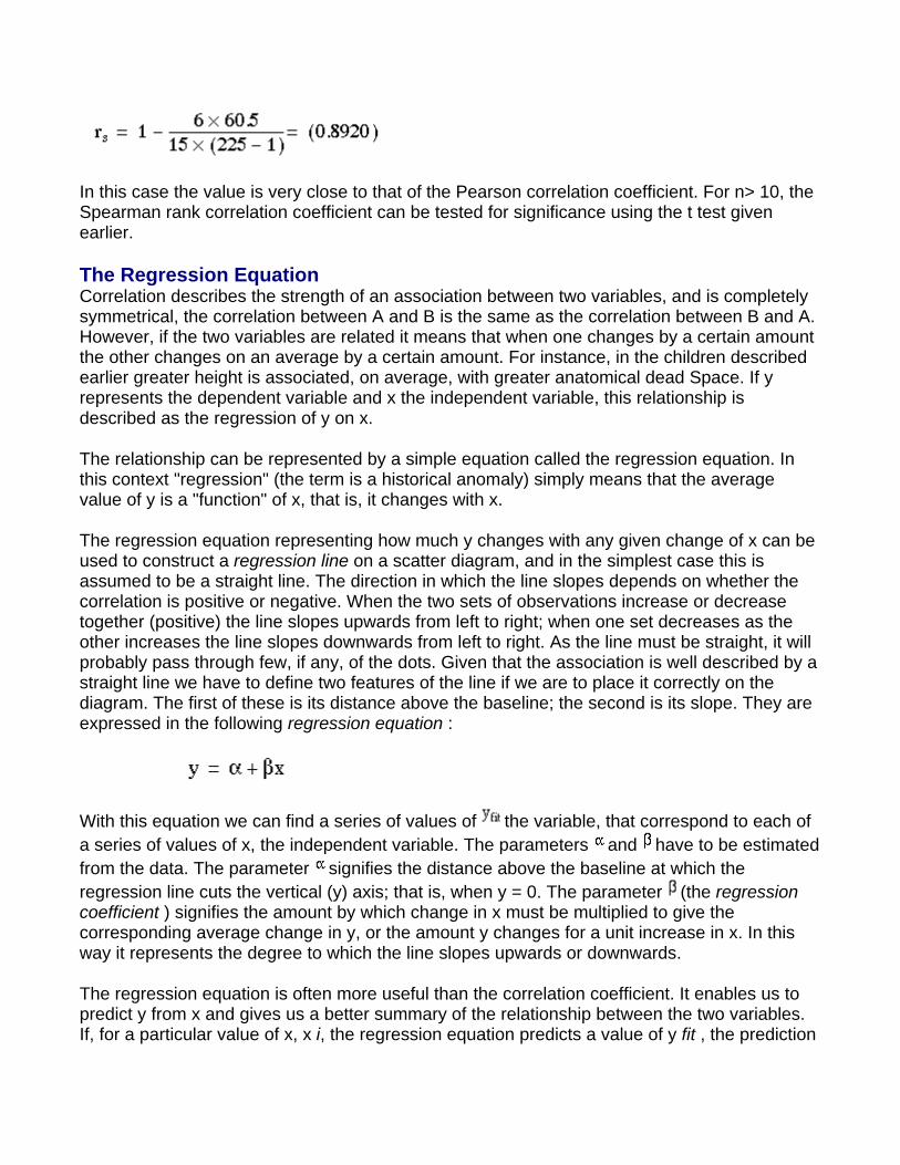
In this case the value is very close to that of the Pearson correlation coefficient. For n> 10, the Spearman rank correlation coefficient can be tested for significance using the t test given earlier.

The Regression Equation Correlation describes the strength of an association between two variables, and is completely symmetrical, the correlation between A and B is the same as the correlation between B and A. However, if the two variables are related it means that when one changes by a certain amount the other changes on an average by a certain amount. For instance, in the children described earlier greater height is associated, on average, with greater anatomical dead Space. If y represents the dependent variable and x the independent variable, this relationship is described as the regression of y on x.

The relationship can be represented by a simple equation called the regression equation. In this context "regression" (the term is a historical anomaly) simply means that the average value of y is a "function" of x, that is, it changes with x.

The regression equation representing how much y changes with any given change of x can be used to construct a regression line on a scatter diagram, and in the simplest case this is assumed to be a straight line. The direction in which the line slopes depends on whether the correlation is positive or negative. When the two sets of observations increase or decrease together (positive) the line slopes upwards from left to right; when one set decreases as the other increases the line slopes downwards from left to right. As the line must be straight, it will probably pass through few, if any, of the dots. Given that the association is well described by a straight line we have to define two features of the line if we are to place it correctly on the diagram. The first of these is its distance above the baseline; the second is its slope. They are expressed in the following regression equation :

With this equation we can find a series of values of the variable, that correspond to each of a series of values of x, the independent variable. The parameters and have to be estimated from the data. The parameter signifies the distance above the baseline at which the regression line cuts the vertical (y) axis; that is, when y = 0. The parameter (the regression coefficient ) signifies the amount by which change in x must be multiplied to give the corresponding average change in y, or the amount y changes for a unit increase in x. In this way it represents the degree to which the line slopes upwards or downwards.

The regression equation is often more useful than the correlation coefficient. It enables us to predict y from x and gives us a better summary of the relationship between the two variables. If, for a particular value of x, x i, the regression equation predicts a value of y fit , the prediction

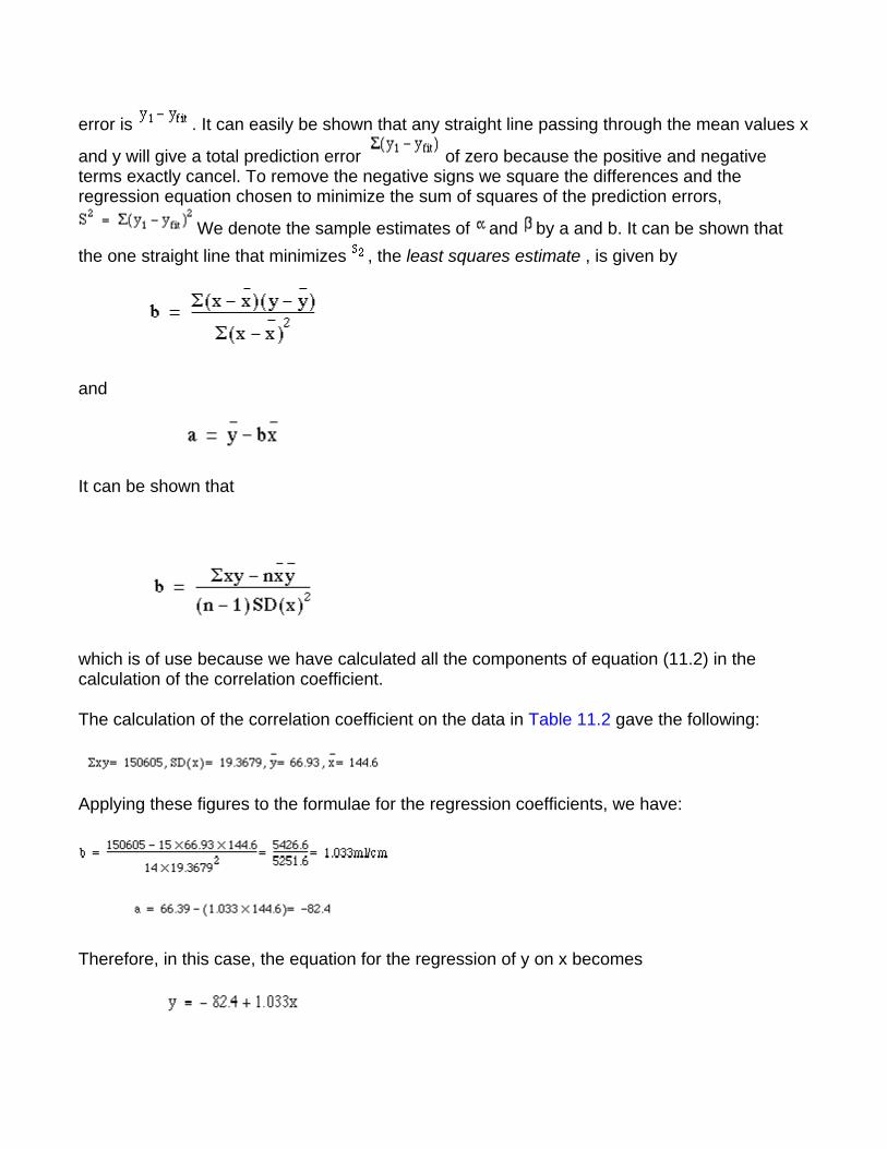
error is . It can easily be shown that any straight line passing through the mean values x

and y will give a total prediction error of zero because the positive and negative terms exactly cancel. To remove the negative signs we square the differences and the regression equation chosen to minimize the sum of squares of the prediction errors,

We denote the sample estimates of and by a and b. It can be shown that the one straight line that minimizes , the least squares estimate , is given by

and

It can be shown that

which is of use because we have calculated all the components of equation (11.2) in the calculation of the correlation coefficient.

The calculation of the correlation coefficient on the data in Table 11.2 gave the following:

Applying these figures to the formulae for the regression coefficients, we have:

Therefore, in this case, the equation for the regression of y on x becomes

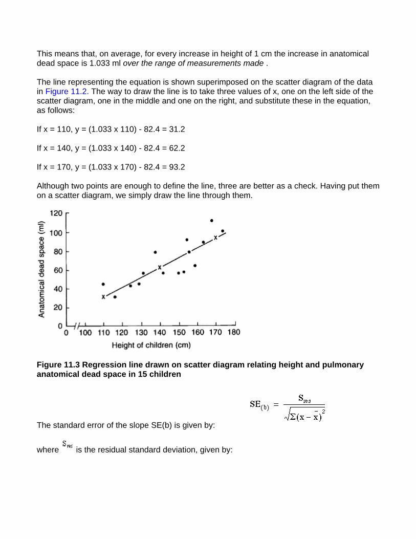
This means that, on average, for every increase in height of 1 cm the increase in anatomical dead space is 1.033 ml over the range of measurements made .

The line representing the equation is shown superimposed on the scatter diagram of the data in Figure 11.2. The way to draw the line is to take three values of x, one on the left side of the scatter diagram, one in the middle and one on the right, and substitute these in the equation, as follows:

If x = 110, y = (1.033 x 110) - 82.4 = 31.2

If x = 140, y = (1.033 x 140) - 82.4 = 62.2

If x = 170, y = (1.033 x 170) - 82.4 = 93.2

Although two points are enough to define the line, three are better as a check. Having put them on a scatter diagram, we simply draw the line through them.

Figure 11.3 Regression line drawn on scatter diagram relating height and pulmonary anatomical dead space in 15 children

The standard error of the slope SE(b) is given by:

where is the residual standard deviation, given by:

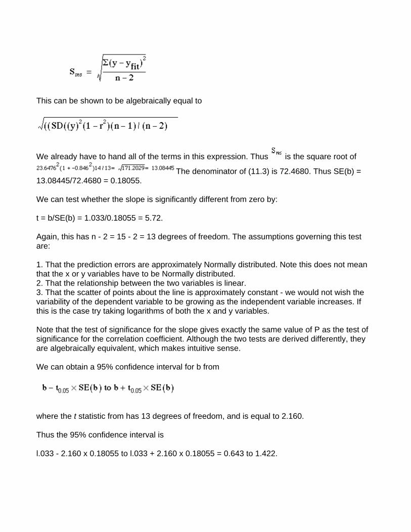
This can be shown to be algebraically equal to

We already have to hand all of the terms in this expression. Thus is the square root of

The denominator of (11.3) is 72.4680. Thus SE(b) = 13.08445/72.4680 = 0.18055.

We can test whether the slope is significantly different from zero by:

t = b/SE(b) = 1.033/0.18055 = 5.72.

Again, this has n - 2 = 15 - 2 = 13 degrees of freedom. The assumptions governing this test are:

1. That the prediction errors are approximately Normally distributed. Note this does not mean that the x or y variables have to be Normally distributed. 2. That the relationship between the two variables is linear. 3. That the scatter of points about the line is approximately constant - we would not wish the variability of the dependent variable to be growing as the independent variable increases. If this is the case try taking logarithms of both the x and y variables.

Note that the test of significance for the slope gives exactly the same value of P as the test of significance for the correlation coefficient. Although the two tests are derived differently, they are algebraically equivalent, which makes intuitive sense.

We can obtain a 95% confidence interval for b from

where the t statistic from has 13 degrees of freedom, and is equal to 2.160.

Thus the 95% confidence interval is

l.033 - 2.160 x 0.18055 to l.033 + 2.160 x 0.18055 = 0.643 to 1.422.

Regression lines give us useful information about the data they are collected from. They show how one variable changes on average with another, and they can be used to find out what one variable is likely to be when we know the other - provided that we ask this question within the limits of the scatter diagram. To project the line at either end - to extrapolate - is always risky because the relationship between x and y may change or some kind of cut off point may exist. For instance, a regression line might be drawn relating the chronological age of some children to their bone age, and it might be a straight line between, say, the ages of 5 and 10 years, but to project it up to the age of 30 would clearly lead to error. Computer packages will often produce the intercept from a regression equation, with no warning that it may be totally meaningless. Consider a regression of blood pressure against age in middle aged men. The regression coefficient is often positive, indicating that blood pressure increases with age. The intercept is often close to zero, but it would be wrong to conclude that this is a reliable estimate of the blood pressure in newly born male infants!

More advanced methods More than one independent variable is possible - in such a case the method is known as multiple regression(3,4). This is the most versatile of statistical methods and can be used in many situations. Examples include: to allow for more than one predictor, age as well as height in the above example; to allow for covariates - in a clinical trial the dependent variable may be outcome after treatment, the first independent variable can be binary, 0 for placebo and 1 for active treatment and the second independent variable may be a baseline variable, measured before treatment, but likely to affect outcome.

Common questions

If two variables are correlated are they causally related? It is a common error to confuse correlation and causation. All that correlation shows is that the two variables are associated. There may be a third variable, a confounding variable that is related to both of them. For example, monthly deaths by drowning and monthly sales of ice-cream are positively correlated, but no-one would say the relationship was causal!

How do I test the assumptions underlying linear regression? Firstly always look at the scatter plot and ask, is it linear? Having obtained the regression equation, calculate the residuals A histogram of will reveal departures from Normality and a plot of versus will reveal whether the residuals increase in size as increases

References

1. Russell MAH, Cole PY, Idle MS, Adams L. Carbon monoxide yields of cigarettes and their relation to nicotine yield and type of filter. BMJ 1975; 3:713.

2. Bland JM, Altman DG. Statistical methods for assessing agreement between two methods of clinical measurement. Lancet 1986; i:307-10.

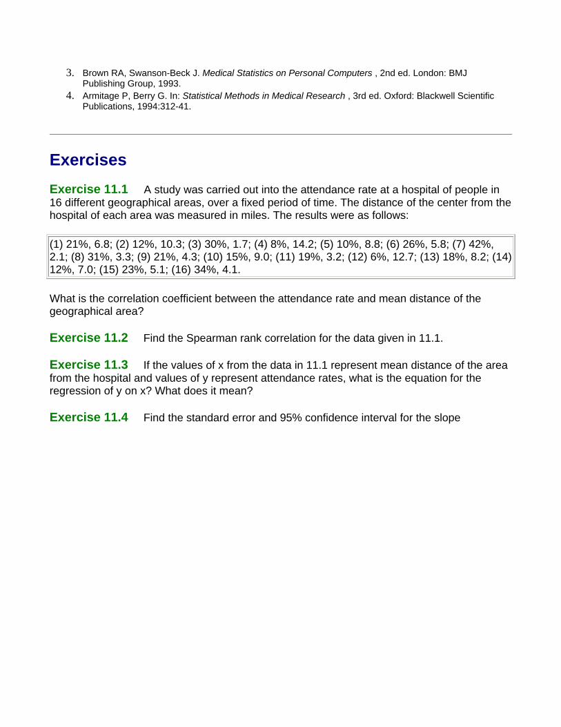
3. Brown RA, Swanson-Beck J. Medical Statistics on Personal Computers , 2nd ed. London: BMJ Publishing Group, 1993.

4. Armitage P, Berry G. In: Statistical Methods in Medical Research , 3rd ed. Oxford: Blackwell Scientific Publications, 1994:312-41.

Exercises

Exercise 11.1 A study was carried out into the attendance rate at a hospital of people in 16 different geographical areas, over a fixed period of time. The distance of the center from the hospital of each area was measured in miles. The results were as follows:

(1) 21%, 6.8; (2) 12%, 10.3; (3) 30%, 1.7; (4) 8%, 14.2; (5) 10%, 8.8; (6) 26%, 5.8; (7) 42%, 2.1; (8) 31%, 3.3; (9) 21%, 4.3; (10) 15%, 9.0; (11) 19%, 3.2; (12) 6%, 12.7; (13) 18%, 8.2; (14) 12%, 7.0; (15) 23%, 5.1; (16) 34%, 4.1.

What is the correlation coefficient between the attendance rate and mean distance of the geographical area?

Exercise 11.2 Find the Spearman rank correlation for the data given in 11.1.

Exercise 11.3 If the values of x from the data in 11.1 represent mean distance of the area from the hospital and values of y represent attendance rates, what is the equation for the regression of y on x? What does it mean?

Exercise 11.4 Find the standard error and 95% confidence interval for the slope

Chapter 12. Survival Analysis

Survival analysis is concerned with studying the time between entry to a study and a subsequent event. Originally the analysis was concerned with time from treatment until death, hence the name, but survival analysis is applicable to many areas as well as mortality. Recent examples include time to discontinuation of a contraceptive, maximum dose of bronchoconstrictor required to reduce a patient's lung function to 80% of baseline, time taken to exercise to maximum tolerance, time that a transdermal patch can be left in place, time for a leg fracture to heal.

When the outcome of a study is the time between one event and another, a number of problems can occur.

1. The times are most unlikely to be Normally distributed. 2. We cannot afford to wait until events have happened to all the subjects, for example until all are dead. Some patients might have left the study early - they are lost to follow up . Thus the only information we have about some patients is that they were still alive at the last follow up. These are termed censored observations .

Kaplan-Meier survival curve We look at the data using a Kaplan-Meier survival curve(1). Suppose that the survival times, including censored observations, after entry into the study (ordered by increasing duration) of a group of n subjects are The proportion of subjects, S(t), surviving beyond any follow

up time ( ) is estimated by

where is the largest survival time less than or equal to t and is the number of subjects alive just before time (the ith ordered survival time), denotes the number who died at time where i can be any value between 1 and p. For censored observations = 0.

Method Order the survival time by increasing duration starting with the shortest one. At each event (i) work out the number alive immediately before the event (r i). Before the first event all the

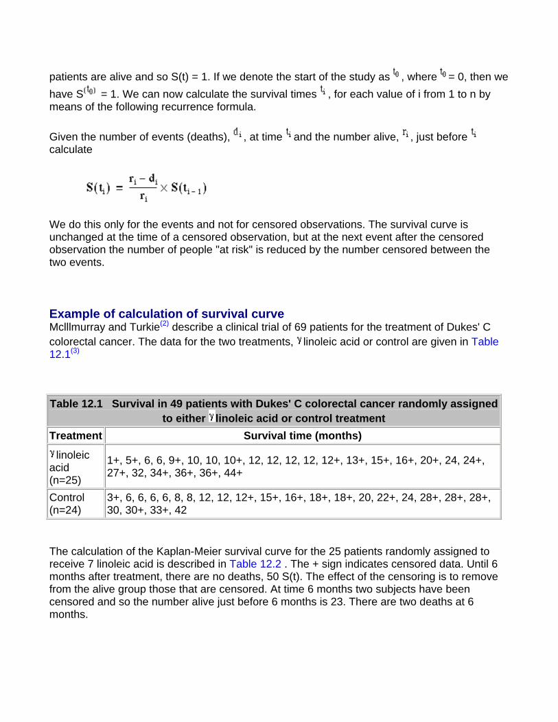
patients are alive and so S(t) = 1. If we denote the start of the study as , where = 0, then we have S = 1. We can now calculate the survival times , for each value of i from 1 to n by means of the following recurrence formula.

Given the number of events (deaths), , at time and the number alive, , just before calculate

We do this only for the events and not for censored observations. The survival curve is unchanged at the time of a censored observation, but at the next event after the censored observation the number of people "at risk" is reduced by the number censored between the two events.

Example of calculation of survival curve Mclllmurray and Turkie(2) describe a clinical trial of 69 patients for the treatment of Dukes' C colorectal cancer. The data for the two treatments, linoleic acid or control are given in Table 12.1(3)

The calculation of the Kaplan-Meier survival curve for the 25 patients randomly assigned to receive 7 linoleic acid is described in Table 12.2 . The + sign indicates censored data. Until 6 months after treatment, there are no deaths, 50 S(t). The effect of the censoring is to remove from the alive group those that are censored. At time 6 months two subjects have been censored and so the number alive just before 6 months is 23. There are two deaths at 6 months.

Table 12.1 Survival in 49 patients with Dukes' C colorectal cancer randomly assigned to either linoleic acid or control treatment

Treatment Survival time (months)

linoleic acid (n=25)

1+, 5+, 6, 6, 9+, 10, 10, 10+, 12, 12, 12, 12, 12+, 13+, 15+, 16+, 20+, 24, 24+, 27+, 32, 34+, 36+, 36+, 44+

Control (n=24)

3+, 6, 6, 6, 6, 8, 8, 12, 12, 12+, 15+, 16+, 18+, 18+, 20, 22+, 24, 28+, 28+, 28+, 30, 30+, 33+, 42

Thus,

S(6)= 1 x (23-2)

23

=0.9130

We now reduce the number alive ("at risk") by two. The censored event at 9 months reduces the "at risk" set to 20. At 10 months there are two deaths, so the proportion surviving is 18/20 = 0.90 and the cumulative proportion surviving is 0.913 x 0.90 = 0.8217. The cumulative survival is conveniently stored in the memory of a calculator. As one can see the effect of the censored observations is to reduce the number at risk without affecting the survival curve S(t).

Table 12.2 Calculation of survival case for 25 patients randomly assigned to receive linoleic acid Case

(i)

Survival time (months)

Number alive

Deaths

Proportion surviving

Cumulative proportion surviving

S(t)

0 0 0 - 1 1 1+ 25 0 1 1 2 5+ 24 0 1 1 3 6 23 2 0.9130 0.9130 4 6 5 9+ 21 0 1 0.9130 6 10 20 2 0.90 0.8217 7 10 8 10+ 9 12 17 4 0.7647 0.6284 10 12 11 12 12 12 13 12+ 14 13+ 12 0 1 0.6284 15 15+ 11 0 1 0.6284

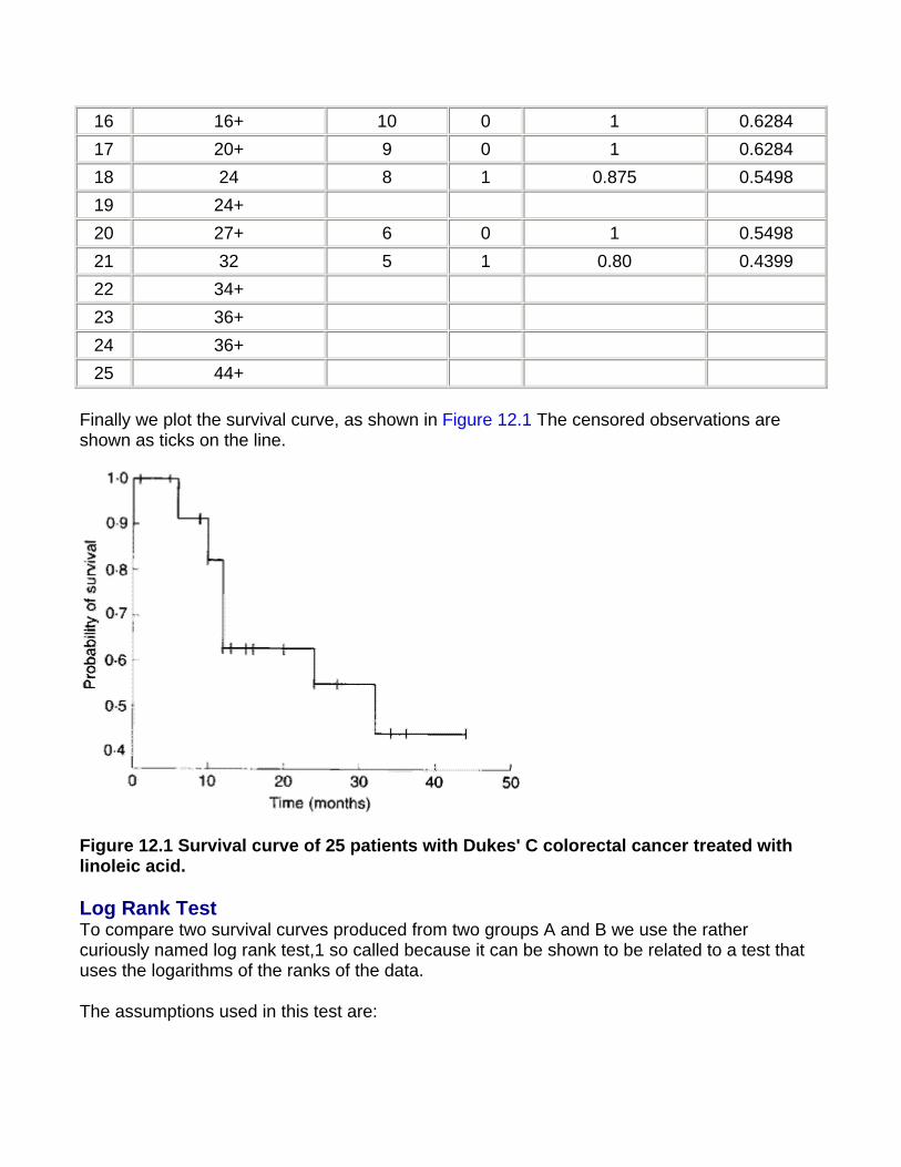
16 16+ 10 0 1 0.6284 17 20+ 9 0 1 0.6284 18 24 8 1 0.875 0.5498 19 24+ 20 27+ 6 0 1 0.5498 21 32 5 1 0.80 0.4399 22 34+ 23 36+ 24 36+ 25 44+

Finally we plot the survival curve, as shown in Figure 12.1 The censored observations are shown as ticks on the line.

Figure 12.1 Survival curve of 25 patients with Dukes' C colorectal cancer treated with linoleic acid.

Log Rank Test To compare two survival curves produced from two groups A and B we use the rather curiously named log rank test,1 so called because it can be shown to be related to a test that uses the logarithms of the ranks of the data.

The assumptions used in this test are:

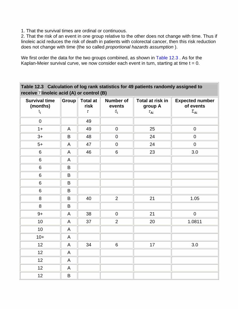
1. That the survival times are ordinal or continuous. 2. That the risk of an event in one group relative to the other does not change with time. Thus if linoleic acid reduces the risk of death in patients with colorectal cancer, then this risk reduction does not change with time (the so called proportional hazards assumption ).

We first order the data for the two groups combined, as shown in Table 12.3 . As for the Kaplan-Meier survival curve, we now consider each event in turn, starting at time t = 0.

Table 12.3 Calculation of log rank statistics for 49 patients randomly assigned to receive linoleic acid (A) or control (B)

Survival time (months)

Group Total at risk

Number of events

Total at risk in group A

Expected number of events

0 49

1+ A 49 0 25 0

3+ B 48 0 24 0

5+ A 47 0 24 0

6 A 46 6 23 3.0

6 A 6 B 6 B 6 B 6 B

8 B 40 2 21 1.05

8 B 9+ A 38 0 21 0

10 A 37 2 20 1.0811

10 A 10+ A 12 A 34 6 17 3.0

12 A 12 A 12 A 12 B

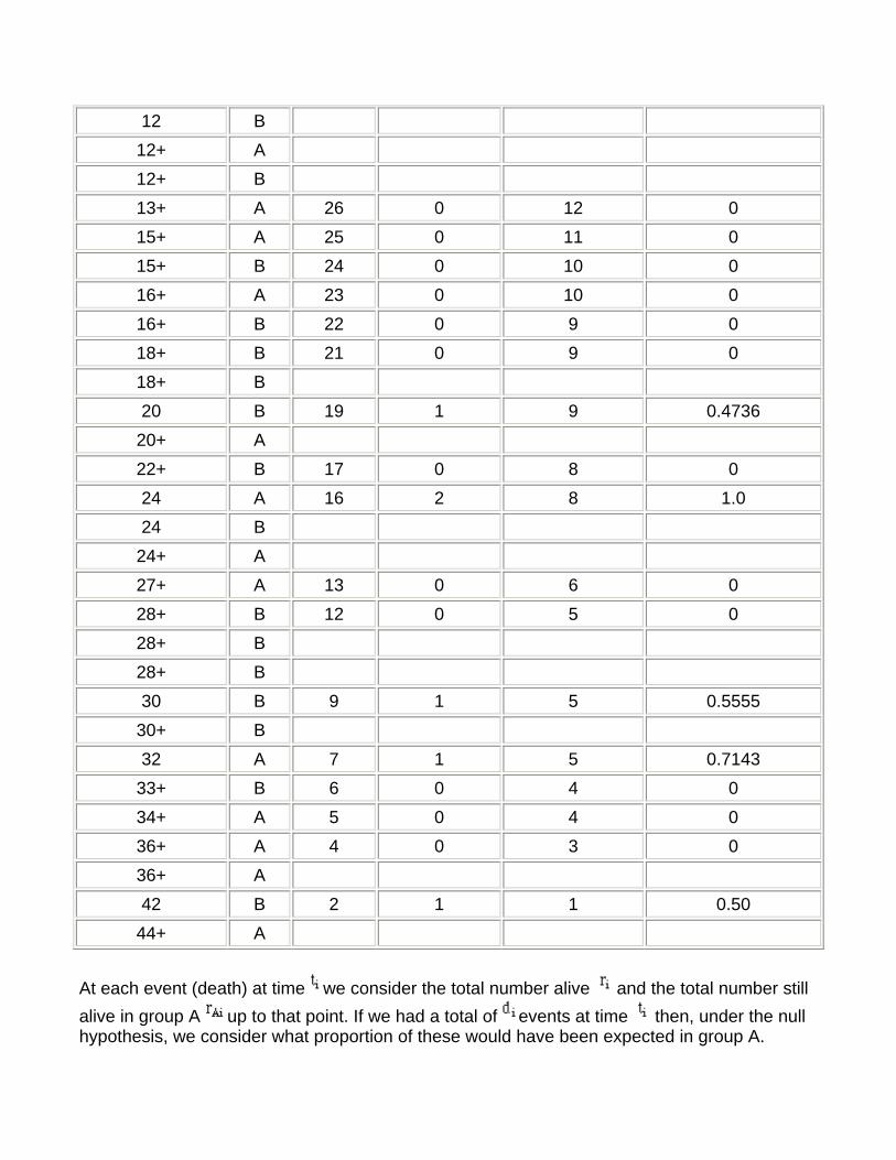
12 B 12+ A 12+ B 13+ A 26 0 12 0

15+ A 25 0 11 0

15+ B 24 0 10 0

16+ A 23 0 10 0

16+ B 22 0 9 0

18+ B 21 0 9 0

18+ B 20 B 19 1 9 0.4736

20+ A 22+ B 17 0 8 0

24 A 16 2 8 1.0

24 B 24+ A 27+ A 13 0 6 0

28+ B 12 0 5 0

28+ B 28+ B 30 B 9 1 5 0.5555

30+ B 32 A 7 1 5 0.7143

33+ B 6 0 4 0

34+ A 5 0 4 0

36+ A 4 0 3 0

36+ A 42 B 2 1 1 0.50

44+ A

At each event (death) at time we consider the total number alive and the total number still alive in group A up to that point. If we had a total of events at time then, under the null hypothesis, we consider what proportion of these would have been expected in group A.

Clearly the more people at risk in one group the more deaths (under the null hypothesis) we would expect.

Thus we obtain

The effect of the censored observations is to reduce the numbers at risk, but they do not contribute to the expected numbers.

Finally, we add the total number of expected events in group A, . If the total number of events in group B is we can deduce from . We do not calculate the expected number beyond the last event, in this case at time 42 months. Also, we would stop calculating the expected values if any survival times greater than the point we were at were found in one group only.

Finally, to test the null hypothesis of equal risk in the two groups we compute

where and are the total number of events in groups A and B. We compare to a distribution with one degree of freedom (one, because we have two groups and one constraint, namely that the total expected events must equal the total observed).

The calculation for the colorectal data is given in Table 12.3. The first non-censored event occurs at 6 months, at which there are six of them. By that time 46 patients are at risk, of whom 23 are in group A. Thus we would expect 6 x 23/46 = 3 to be in group A. At 8 months we have 46 - 6 = 40 patients at risk of whom 23 - 2 = 21 are in group A. There are two events, of which we would expect 2 x 21/40 = 1.05 to occur in group A.

The total expected number of events in A is = 11.3745. The total number of events is 22, = 10, = 12. Thus =10.6255.

Thus

We compare this with the Table given in Appendix E, to find that P>0.10.

The relative risk can be estimated by . The standard error of the log risk is given by (4)

Thus we find r = 0.78 and so log(r) = -0.248.

SE(log(r)) = 0.427, and so an approximate 95% confidence interval for log(r) is

-1.10 to 0.605 and so a 95% confidence interval for r is , which is

0.33 to 1.83.

This would imply that linoleic acid reduced mortality by about 78% compared with the control

group, but with a very wide confidence interval. In view of the very small statistic, we have little evidence that this result would not have arisen by chance.

Further methods In the same way that multiple regression is an extension of linear regression, an extension of the log rank test includes, for example, allowance for prognostic factors. This was developed by DR Cox, and so is called Cox regression . It is beyond the scope of this book, but is described elsewhere(4, 5).

Common questions

Do I need to test for a constant relative risk before doing the log rank test? This is a similar problem to testing for Normality for a t test. The log rank test is quite "robust" against departures from proportional hazards, but care should be taken. If the Kaplan-Meier survival curves cross then this is clear departure from proportional hazards, and the log rank test should not be used. This can happen, for example, in a two drug trial for cancer, if one drug is very toxic initially but produces more long term cures. In this case there is no simple answer to the question "is one drug better than the other?", because the answer depends on the time scale.

If I don't have any censored observations, do I need to use survival analysis? Not necessarily, you could use a rank test such as the Mann-Whitney U test, but the survival method would yield an estimate of risk, which is often required, and lends itself to a useful way of displaying the data.

References

1. Peto R, Pike MC, Armitage P et al . Design and analysis of randomized clinical trials requiring prolonged observation of each patient: II. Analysis and examples. Br J Cancer l977; 35 :l-39.

2. McIllmurray MB, Turkie W. Controlled trial of linoleic acid in Dukes' C colorectal cancer. BMJ 1987; 294 :1260, 295 :475.

3. Gardner MJ, Altman DG (Eds). In: Statistics with Confidence, Confidence Intervals and Statistical Guidelines . London: BMJ Publishing Group, 1989; Chapter 7.

4. Armitage P, Berry G. In: Statistical Methods in Medical Practice . Oxford: Blackwell Scientific Publications, 1994:477-81.

5. Altman DG. Practical Statistics for Medical Research .. London: Chapman & Hall, 1991.

Exercises

Exercise 12.1 Twenty patients, ten of normal weight and ten severely overweight underwent an exercise stress test, in which they had to lift a progressively increasing load for up to 12 minutes, but they were allowed to stop earlier if they could do no more. On two occasions the equipment failed before 12 minutes. The times (in minutes) achieved were:

Normal weight: 4, 10, 12*, 2, 8, 12*, 8**, 6, 9, 12*

Overweight: 7**, 5, 11, 6, 3, 9, 4, 1, 7, 12*

*Reached end of test; **equipment failure. What are the observed and expected values? What is the value of the log rank test to compare these groups?

Exercise 12.2 What is the risk of stopping in the normal weight group compared with the overweight group, and a 95% confidence interval?

Chapter 13. Study Design and Choosing

a Statistical Test

Study Design In many ways the design of a study is more important than the analysis. A badly designed study can never be retrieved, whereas a poorly analyzed one can usually be reanalyzed(1). Consideration of design is also important because the design of a study will govern how the data are to be analyzed.

Most medical studies consider an input, which may be a medical intervention or exposure to a potentially toxic compound, and an output, which is some measure of health that the intervention is supposed to affect. The simplest way to categorize studies is with reference to the time sequence in which the input and output are studied.

The most powerful studies are prospective studies, and the paradigm for these is the randomized controlled trial. In this subjects with a disease are randomized to one of two (or more) treatments, one of which may be a control treatment. Methods of randomization have been described in Chapter 3. The importance of randomization is that we know in the long run treatment groups will be balanced in known and unknown prognostic factors. It is important that the treatments are concurrent - that the active and control treatments occur in the same period of time.

A parallel group design is one in which treatment and control are allocated to different individuals. To allow for the therapeutic effect of simply being given treatment, the control may consist of a placebo, an inert substance that is physically identical to the active compound. If possible a study should be double blinded - neither the investigator nor the subject being aware of what treatment the subject is undergoing. Sometimes it is impossible to blind the subjects, for example when the treatment is some form of health education, but often it is possible to ensure that the people evaluating the outcome are unaware of the treatment. An example of a parallel group trial is given in Table 7.1, in which different bran preparations have been tested on different individuals.

A matched design comes about when randomization is between matched pairs, such as in Exercise 6.2, in which randomization was between different parts of a patient's body.

A crossover study is one in which two or more treatments are applied sequentially to the same subject. The advantages are that each subject then acts as their own control and so fewer subjects may be required. The main disadvantage is that there may be a carry over effect in that the action of the second treatment is affected by the first treatment. An example of a crossover trial is given in Table 7.2, in which different dosages of bran are compared within the same individual. A number of excellent books are available on clinical trials.(2, 3)

One of the major threats to validity of a clinical trial is compliance. Patients are likely to drop out of trials if the treatment is unpleasant, and often fail to take medication as prescribed. It is usual to adopt a pragmatic approach and analyze by intention to treat , that is analyze the study by the treatment that the subject was assigned to, not the one they actually took. The alternative is to analyze per protocol or on study . Drop outs should of course be reported by treatment group. A checklist for writing reports on clinical trials is available.(4, 5)

A quasi experimental design is one in which treatment allocation is not random. An example of this is given in Table 9.1 in which injuries are compared in two dropping zones. This is subject to potential biases in that the reason why a person is allocated to a particular dropping zone may be related to their risk of a sprained ankle.

A cohort study is one in which subjects, initially disease free, are followed up over a period of time. Some will be exposed to some risk factor, for example cigarette smoking. The outcome may be death and we may be interested in relating the risk factor to a particular cause of death. Clearly, these have to be large, long term studies and tend to be costly to carry out. If records have been kept routinely in the past then a historical cohort study may be carried out, an example of which is the appendicitis study discussed in Chapter 6. Here, the cohort is all cases of appendicitis admitted over a given period and a sample of the records could be inspected retrospectively. A typical example would be to look at birth weight records and relate birth weight to disease in later life.

These studies differ in essence from retrospective studies, which start with diseased subjects and then examine possible exposure. Such case control studies are commonly undertaken as a preliminary investigation, because they are relatively quick and inexpensive. The comparison of the blood pressure in farmers and printers given in Chapter 3 is an example of a case control study. It is retrospective because we argued from the blood pressure to the occupation and did not start out with subjects assigned to occupation. There are many confounding factors in case control studies. For example, does occupational stress cause high blood pressure, or do people prone to high blood pressure choose stressful occupations? A particular problem is recall bias, in that the cases, with the disease, are more motivated to recall apparently trivial episodes in the past than controls, who are disease free.

Cross sectional studies are common and include surveys, laboratory experiments and studies to examine the prevalence of a disease. Studies validating instruments and questionnaires are also cross sectional studies. The study of urinary concentration of lead in children described in Chapter 1 and the study of the relationship between height and pulmonary anatomical dead space in Chapter 11 were also cross sectional studies.

Sample size One of the most common questions asked of a statistician about design is the number of patients to include. It is an important question, because if a study is too small it will not be able to answer the question posed, and would be a waste of time and money. It could also be deemed unethical because patients may be put at risk with no apparent benefit. However, studies should not be too large because resources would be wasted if fewer patients would have sufficed. The sample size depends on four critical quantities: the type I and type II error

rates and (discussed in Chapter 5), the variability of the data , and the effect size d. In a trial the effect size is the amount by which we would expect the two treatments to differ, or is the difference that would be clinically worthwhile.

Usually and are fixed at 5% and 20% (or 10%) respectively. A simple formula for a two group parallel trial with a continuous outcome is that the required sample size per group is

given by for two sided of 5% and of 20%. For example, in a trial to reduce blood pressure, if a clinically worthwhile effect for diastolic blood pressure is 5 mmHg and the between subjects standard deviation is 10 mmHg, we would require n = 16 x 100/25 = 64 patients per group in the study. The sample size goes up as the square of the standard deviation of the data (the variance) and goes down inversely as the square of the effect size. Doubling the effect size reduces the sample size by four - it is much easier to detect large effects! In practice, the sample size is often fixed by other criteria, such as finance or resources, and the formula is used to determine a realistic effect size. If this is too large, then the study will have to be abandoned or increased in size. Machin et al. give advice on a sample size calculations for a wide variety of study designs.(6)

Choice of test In terms of selecting a statistical test, the most important question is "what is the main study hypothesis?" In some cases there is no hypothesis; the investigator just wants to "see what is there". For example, in a prevalence study there is no hypothesis to test, and the size of the study is determined by how accurately the investigator wants to determine the prevalence. If there is no hypothesis, then there is no statistical test. It is important to decide a priori which hypotheses are confirmatory (that is, are testing some presupposed relationship), and which are exploratory (are suggested by the data). No single study can support a whole series of hypotheses.

A sensible plan is to limit severely the number of confirmatory hypotheses. Although it is valid to use statistical tests on hypotheses suggested by the data, the P values should be used only as guidelines, and the results treated as very tentative until confirmed by subsequent studies. A useful guide is to use a Bonferroni correction, which states simply that if one is testing n independent hypotheses, one should use a significance level of 0.05/n. Thus if there were two independent hypotheses a result would be declared significant only if P<0.025. Note that, since

tests are rarely independent, this is a very conservative procedure - one unlikely to reject the null hypothesis.

The investigator should then ask "are the data independent?" This can be difficult to decide but as a rule of thumb results on the same individual, or from matched individuals, are not independent. Thus results from a crossover trial, or from a case control study in which the controls were matched to the cases by age, sex and social class, are not independent. It is generally true that the analysis should reflect the design, and so a matched design should be followed by a matched analysis. Results measured over time require special care.(7) One of the most common mistakes in statistical analysis is to treat dependent variables as independent. For example, suppose we were looking at treatment of leg ulcers, in which some people had an ulcer on each leg. We might have 20 subjects with 30 ulcers but the number of independent pieces of information is 20 because the state of an ulcer on one leg may influence the state of the ulcer on the other leg and an analysis that considered ulcers as independent observations would be incorrect. For a correct analysis of mixed paired and unpaired data consult a statistician.

The next question is "what types of data are being measured?" The test used should be determined by the data. The choice of test for matched or paired data is described in and for independent data in .

Choice of statistical test from paired or matched observation

Variable Test Nominal McNemar's Test Ordinal (Ordered categories) Wilcoxon Quantitative (Discrete or Non-Normal) Wilcoxon Quantitative (Normal*) Paired t test * It is the difference between the paired observations that should be plausibly Normal.

It is helpful to decide the input variables and the outcome variables. For example in a clinical trial the input variable is type of treatment - a nominal variable - and the outcome may be some clinical measure perhaps Normally distributed. The required test is then the t test (Table 13.2). However, if the input variable is continuous, say a clinical score, and the outcome is nominal, say cured or not cured, logistic regression is the required analysis. A t test in this case may help but would not give us what we require, namely the probability of a cure for a given value of the clinical score. As another example, suppose we have a cross sectional study in which we ask a random sample of people whether they think their general practitioner is doing a good job, on a five point scale, and we wish to ascertain whether women have a higher opinion of general practitioners than men have. The input variable is gender, which is nominal. The outcome variable is the five point ordinal scale. Each person's opinion is independent of the

others, so we have independent data. From we should use a test for trend, or a Mann-Whitney U test (with correction for ties). Note, however, if some people share a general

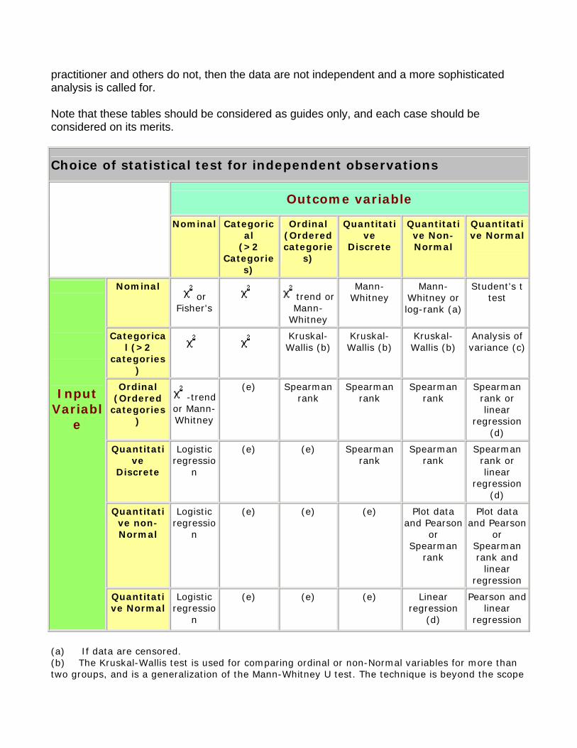
practitioner and others do not, then the data are not independent and a more sophisticated analysis is called for.

Note that these tables should be considered as guides only, and each case should be considered on its merits.

Choice of statistical test for independent observations

Outcome variable

Nominal Categorical

(>2 Categorie

s)

Ordinal (Ordered categorie

s)

Quantitative

Discrete

Quantitative Non-Normal

Quantitative Normal

Nominal or

Fisher's trend or

Mann-Whitney

Mann-Whitney

Mann-Whitney or log-rank (a)

Student's t test

Categorical (>2

categories)

Kruskal-Wallis (b)

Kruskal-Wallis (b)

Kruskal-Wallis (b)

Analysis of variance (c)

Ordinal (Ordered

categories)

-trend or Mann- Whitney

(e) Spearman rank

Spearman rank

Spearman rank

Spearman rank or linear

regression (d)

Quantitative

Discrete

Logistic regressio

n

(e) (e) Spearman rank

Spearman rank

Spearman rank or linear

regression (d)

Quantitative non-Normal

Logistic regressio

n

(e)

(e)

(e)

Plot data and Pearson

or Spearman

rank

Plot data and Pearson

or Spearman rank and

linear regression

Input Variabl

e

Quantitative Normal

Logistic regressio

n

(e)

(e)

(e)

Linear regression

(d)

Pearson and linear

regression

(a) If data are censored. (b) The Kruskal-Wallis test is used for comparing ordinal or non-Normal variables for more than two groups, and is a generalization of the Mann-Whitney U test. The technique is beyond the scope

of this paper, but is described in more advanced books and is available in common software (Epi-Info, Minitab, SPSS). (c) Analysis of variance is a general technique, and one version (one way analysis of variance) is used to compare Normally distributed variables for more than two groups, and is the parametric equivalent of the Kruskal-Wallis test. (d) If the outcome variable is the dependent variable, then provided the residuals (see ) are plausibly Normal, then the distribution of the independent variable is not important. (e) There are a number of more advanced techniques, such as Poisson regression, for dealing with these situations. However, they require certain assumptions and it is often easier to either dichotomize the outcome variable or treat it as continuous.

References

1. Campbell MJ, Machin D. In: Medical Statistics: A Common-sense Approach , 2nd ed. Chichester: Wiley, 1993:2.

2. Pocock SJ. Clinical trials: A Practical Approach . Chichester: Wiley, 1982. 3. Senn SJ. The Design and Analysis of Cross-Over Trials . Chichester: Wiley, 1992. 4. Gardner MJ, Altman DG (eds) In: Statistics with Confidence . BMJ Publishing Group, 1989:103-5. 5. Gardner MJ, Machin D, Campbell MJ. The use of checklists in assessing the statistical content of medical

studies. BMJ 1986; 292 :810-12. 6. Macbin D, Campbell MJ, Payers P, Pinol A. Statistical Tables for the Design of Clinical Studies . Oxford:

Blackwell Scientific Publications, 1996. 7. Matthews JNS, Altman DG, Campbell MJ, Royston JP. Analysis of senal measurements in medical

research. BMJ 1990; 300 :230-5. 8. Altman DG. Practical Statistics for Medical Research . London: Chapman & Hall, 1991. 9. Armitage P, Berry G. In: Statistical Methods in Medical Research . Oxford: Blackwell Scientific

Publications, 1994.

Exercises

State the type of study described in each of the following.

Exercise 13.1 To investigate the relationship between egg consumption and heart disease, a group of patients admitted to hospital with myocardial infarction were questioned about their egg consumption. A group of age and sex matched patients admitted to a fracture clinic were also questioned about their egg consumption using an identical protocol.

Exercise 13.2 To investigate the relationship between certain solvents and cancer, all employees at a factory were questioned about their exposure to an industrial solvent, and the amount and length of exposure measured. These subjects were regularly monitored, and after 10 years a copy of the death certificate for all those who had died was obtained.

Exercise 13.3 A survey was conducted of all nurses employed at a particular hospital. Among other questions, the questionnaire asked about the grade of the nurse and whether she was satisfied with her career prospects.

Exercise 13.4 To evaluate a new back school, patients with lower back pain were randomly allocated to either the new school or to conventional occupational therapy. After 3 months they were questioned about their back pain, and observed lifting a weight by independent monitors.

Exercise 13.5 A new triage system has been set up at the local Accident and Emergency Unit. To evaluate it the waiting times of patients were measured for 6 months and compared with the waiting times at a comparable nearby hospital.

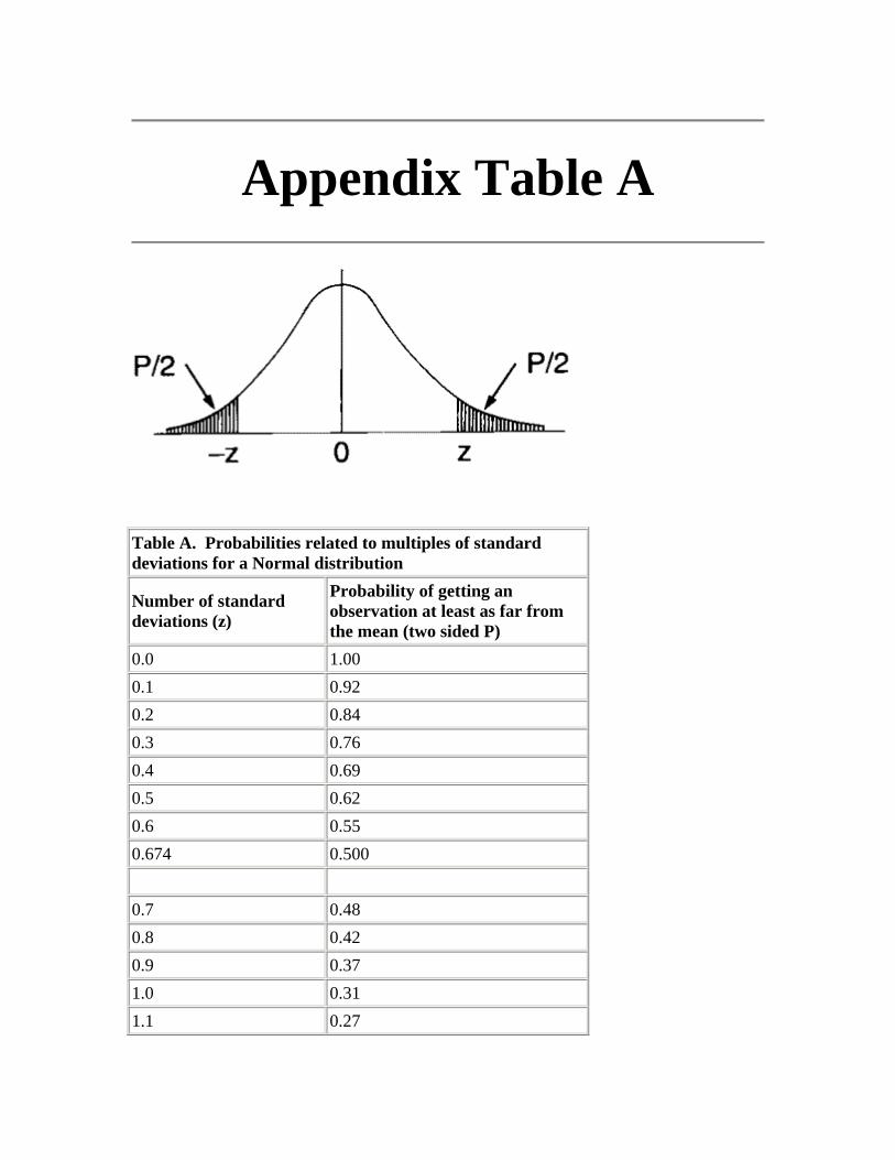
Appendix Table A

Table A. Probabilities related to multiples of standard deviations for a Normal distribution

Number of standard deviations (z)

Probability of getting an observation at least as far from the mean (two sided P)

0.0 1.00 0.1 0.92 0.2 0.84 0.3 0.76 0.4 0.69 0.5 0.62 0.6 0.55 0.674 0.500 0.7 0.48 0.8 0.42 0.9 0.37 1.0 0.31 1.1 0.27

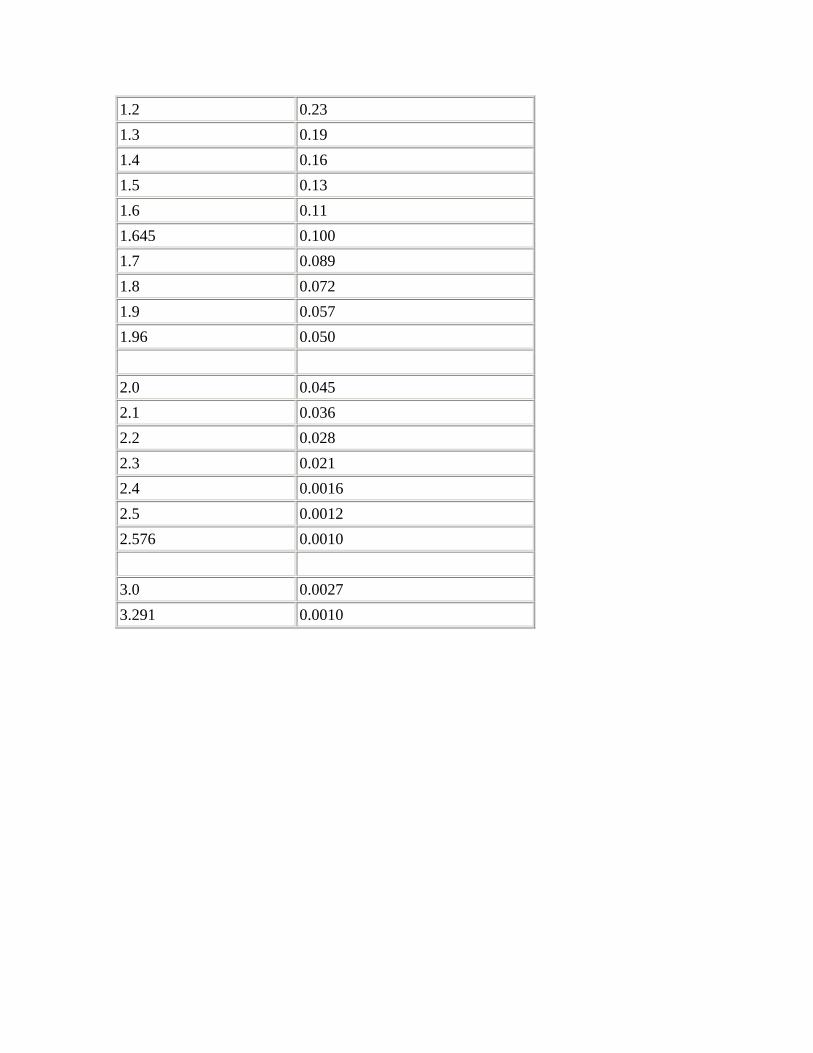
1.2 0.23 1.3 0.19 1.4 0.16 1.5 0.13 1.6 0.11 1.645 0.100 1.7 0.089 1.8 0.072 1.9 0.057 1.96 0.050 2.0 0.045 2.1 0.036 2.2 0.028 2.3 0.021 2.4 0.0016 2.5 0.0012 2.576 0.0010 3.0 0.0027 3.291 0.0010

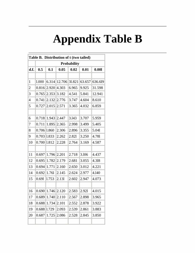
Appendix Table B

Table B. Distribution of t (two tailed)

Probability d.f. 0.5 0.1 0.05 0.02 0.01 0.00l 1 l.000 6.314 12.706 3l.821 63.657 636.6l92 0.816 2.920 4.303 6.965 9.925 31.5983 0.765 2.353 3.182 4.541 5.841 12.9414 0.741 2.132 2.776 3.747 4.604 8.610 5 0.727 2.015 2.571 3.365 4.032 6.859 6 0.718 1.943 2.447 3.l43 3.707 5.959 7 0.711 1.895 2.365 2.998 3.499 5.405 8 0.706 l.860 2.306 2.896 3.355 5.04l 9 0.703 l.833 2.262 2.82l 3.250 4.78l 10 0.700 l.812 2.228 2.764 3.169 4.587 11 0.697 1.796 2.201 2.718 3.l06 4.437 12 0.695 1.782 2.179 2.681 3.055 4.3l8 13 0.694 1.771 2.160 2.650 3.012 4.221 14 0.692 1.76l 2.145 2.624 2.977 4.l40 15 0.69l l.753 2.13l 2.602 2.947 4.073 16 0.690 1.746 2.120 2.583 2.92l 4.015 17 0.689 1.740 2.110 2.567 2.898 3.965 18 0.688 1.734 2.101 2.552 2.878 3.922 19 0.688 l.729 2.093 2.539 2.861 3.883 20 0.687 1.725 2.086 2.528 2.845 3.850

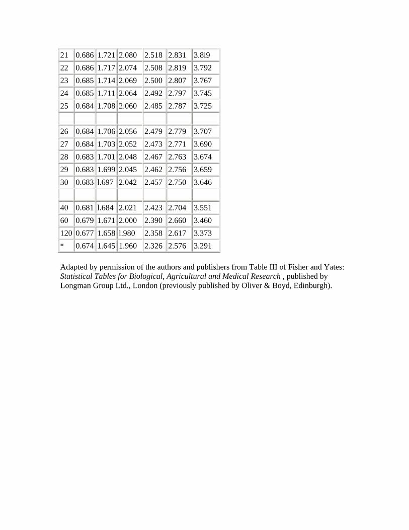
21 0.686 1.721 2.080 2.518 2.831 3.8l9 22 0.686 1.717 2.074 2.508 2.819 3.792 23 0.685 1.714 2.069 2.500 2.807 3.767 24 0.685 1.711 2.064 2.492 2.797 3.745 25 0.684 1.708 2.060 2.485 2.787 3.725 26 0.684 1.706 2.056 2.479 2.779 3.707 27 0.684 1.703 2.052 2.473 2.771 3.690 28 0.683 1.701 2.048 2.467 2.763 3.674 29 0.683 1.699 2.045 2.462 2.756 3.659 30 0.683 l.697 2.042 2.457 2.750 3.646 40 0.681 l.684 2.021 2.423 2.704 3.551 60 0.679 1.671 2.000 2.390 2.660 3.460 120 0.677 1.658 l.980 2.358 2.617 3.373

0.674 1.645 1.960 2.326 2.576 3.291

Adapted by permission of the authors and publishers from Table III of Fisher and Yates: Statistical Tables for Biological, Agricultural and Medical Research , published by Longman Group Ltd., London (previously published by Oliver & Boyd, Edinburgh).

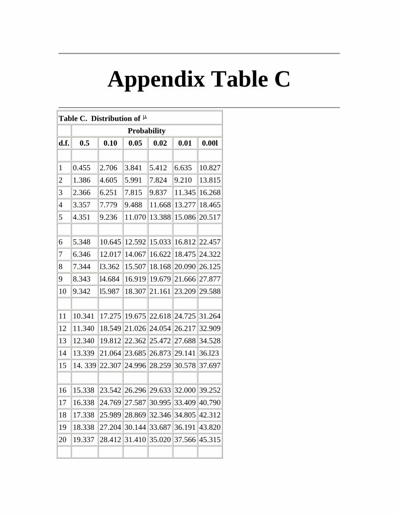
Appendix Table C

Table C. Distribution of

Probability d.f. 0.5 0.10 0.05 0.02 0.01 0.00l 1 0.455 2.706 3.841 5.412 6.635 10.8272 1.386 4.605 5.991 7.824 9.210 13.8153 2.366 6.251 7.815 9.837 11.345 16.2684 3.357 7.779 9.488 11.668 13.277 18.4655 4.351 9.236 11.070 13.388 15.086 20.517 6 5.348 10.645 12.592 15.033 16.812 22.4577 6.346 12.017 14.067 16.622 18.475 24.3228 7.344 l3.362 15.507 18.168 20.090 26.1259 8.343 l4.684 16.919 19.679 21.666 27.87710 9.342 l5.987 18.307 21.161 23.209 29.588 11 10.341 17.275 19.675 22.618 24.725 31.26412 11.340 18.549 21.026 24.054 26.217 32.90913 12.340 19.812 22.362 25.472 27.688 34.52814 13.339 21.064 23.685 26.873 29.141 36.l2315 14. 339 22.307 24.996 28.259 30.578 37.697 16 15.338 23.542 26.296 29.633 32.000 39.25217 16.338 24.769 27.587 30.995 33.409 40.79018 17.338 25.989 28.869 32.346 34.805 42.31219 18.338 27.204 30.144 33.687 36.191 43.82020 19.337 28.412 31.410 35.020 37.566 45.315

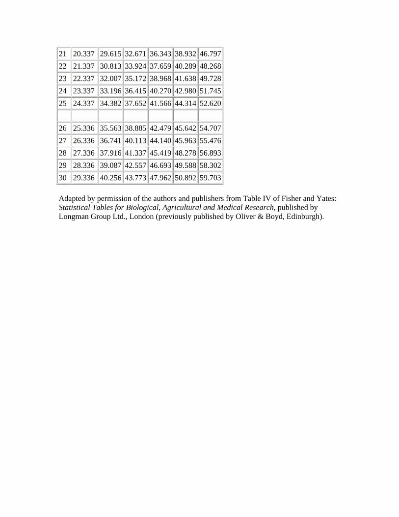
21 20.337 29.615 32.671 36.343 38.932 46.79722 21.337 30.813 33.924 37.659 40.289 48.26823 22.337 32.007 35.172 38.968 41.638 49.72824 23.337 33.196 36.415 40.270 42.980 51.74525 24.337 34.382 37.652 41.566 44.314 52.620 26 25.336 35.563 38.885 42.479 45.642 54.70727 26.336 36.741 40.113 44.140 45.963 55.47628 27.336 37.916 41.337 45.419 48.278 56.89329 28.336 39.087 42.557 46.693 49.588 58.30230 29.336 40.256 43.773 47.962 50.892 59.703

Adapted by permission of the authors and publishers from Table IV of Fisher and Yates: Statistical Tables for Biological, Agricultural and Medical Research, published by Longman Group Ltd., London (previously published by Oliver & Boyd, Edinburgh).

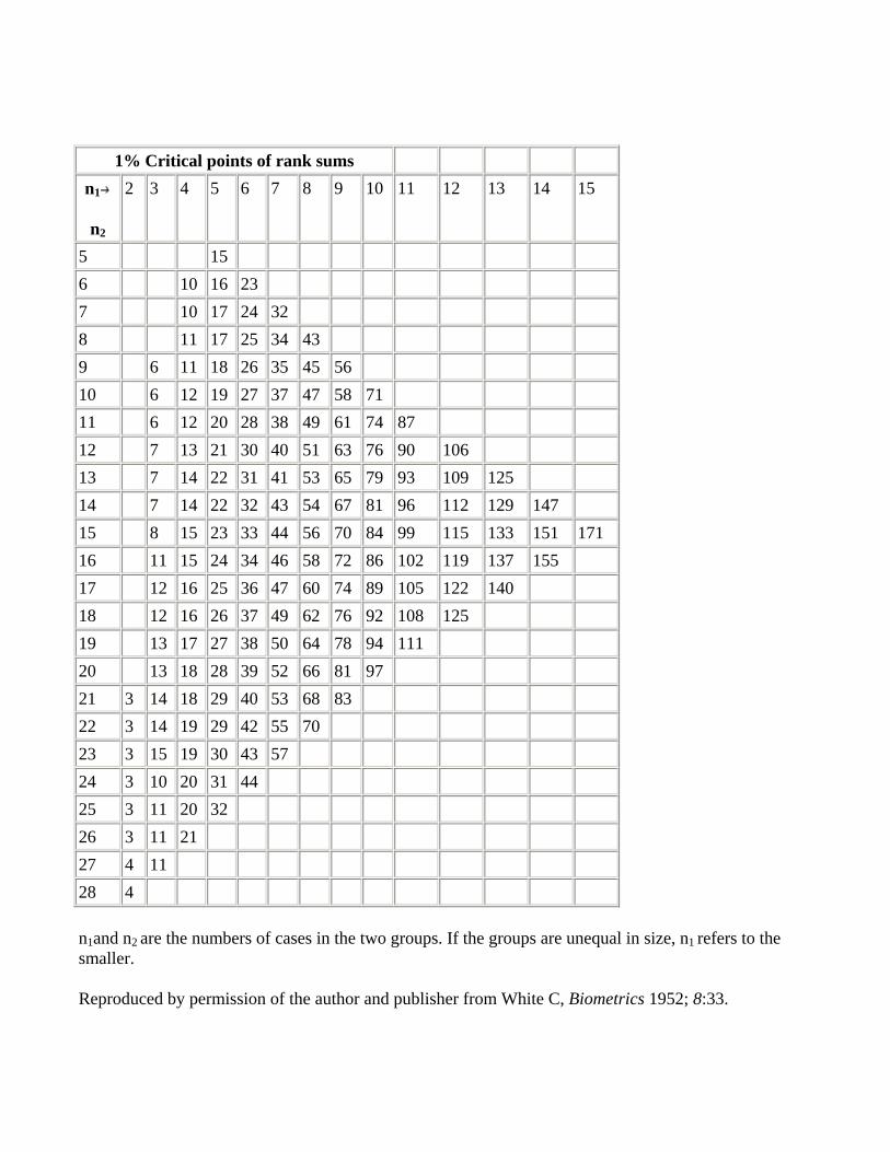
1% Critical points of rank sums n1

n2

2 3 4 5 6 7 8 9 10 11 12 13 14 15

5 15 6 10 16 23 7 10 17 24 32 8 11 17 25 34 43 9 6 11 18 26 35 45 56 10 6 12 19 27 37 47 58 71 11 6 12 20 28 38 49 61 74 87 12 7 13 21 30 40 51 63 76 90 106 13 7 14 22 31 41 53 65 79 93 109 125 14 7 14 22 32 43 54 67 81 96 112 129 147 15 8 15 23 33 44 56 70 84 99 115 133 151 171 16 11 15 24 34 46 58 72 86 102 119 137 155 17 12 16 25 36 47 60 74 89 105 122 140 18 12 16 26 37 49 62 76 92 108 125 19 13 17 27 38 50 64 78 94 111 20 13 18 28 39 52 66 81 97 21 3 14 18 29 40 53 68 83 22 3 14 19 29 42 55 70 23 3 15 19 30 43 57 24 3 10 20 31 44 25 3 11 20 32 26 3 11 21 27 4 11 28 4

n1and n2 are the numbers of cases in the two groups. If the groups are unequal in size, n1 refers to the smaller.

Reproduced by permission of the author and publisher from White C, Biometrics 1952; 8:33.

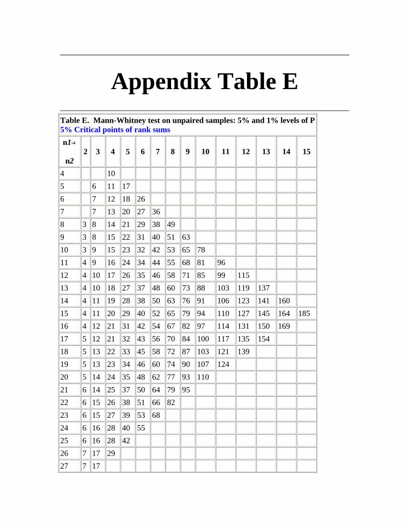
Appendix Table E

Table E. Mann-Whitney test on unpaired samples: 5% and 1% levels of P 5% Critical points of rank sums n1

n2 2 3 4 5 6 7 8 9 10 11 12 13 14 15

4 10 5 6 11 17 6 7 12 18 26 7 7 13 20 27 36 8 3 8 14 21 29 38 49 9 3 8 15 22 31 40 51 63 10 3 9 15 23 32 42 53 65 78 11 4 9 16 24 34 44 55 68 81 96 12 4 10 17 26 35 46 58 71 85 99 115 13 4 10 18 27 37 48 60 73 88 103 119 137 14 4 11 19 28 38 50 63 76 91 106 123 141 160 15 4 11 20 29 40 52 65 79 94 110 127 145 164 185 16 4 12 21 31 42 54 67 82 97 114 131 150 169 17 5 12 21 32 43 56 70 84 100 117 135 154 18 5 13 22 33 45 58 72 87 103 121 139 19 5 13 23 34 46 60 74 90 107 124 20 5 14 24 35 48 62 77 93 110 21 6 14 25 37 50 64 79 95 22 6 15 26 38 51 66 82 23 6 15 27 39 53 68 24 6 16 28 40 55 25 6 16 28 42 26 7 17 29 27 7 17

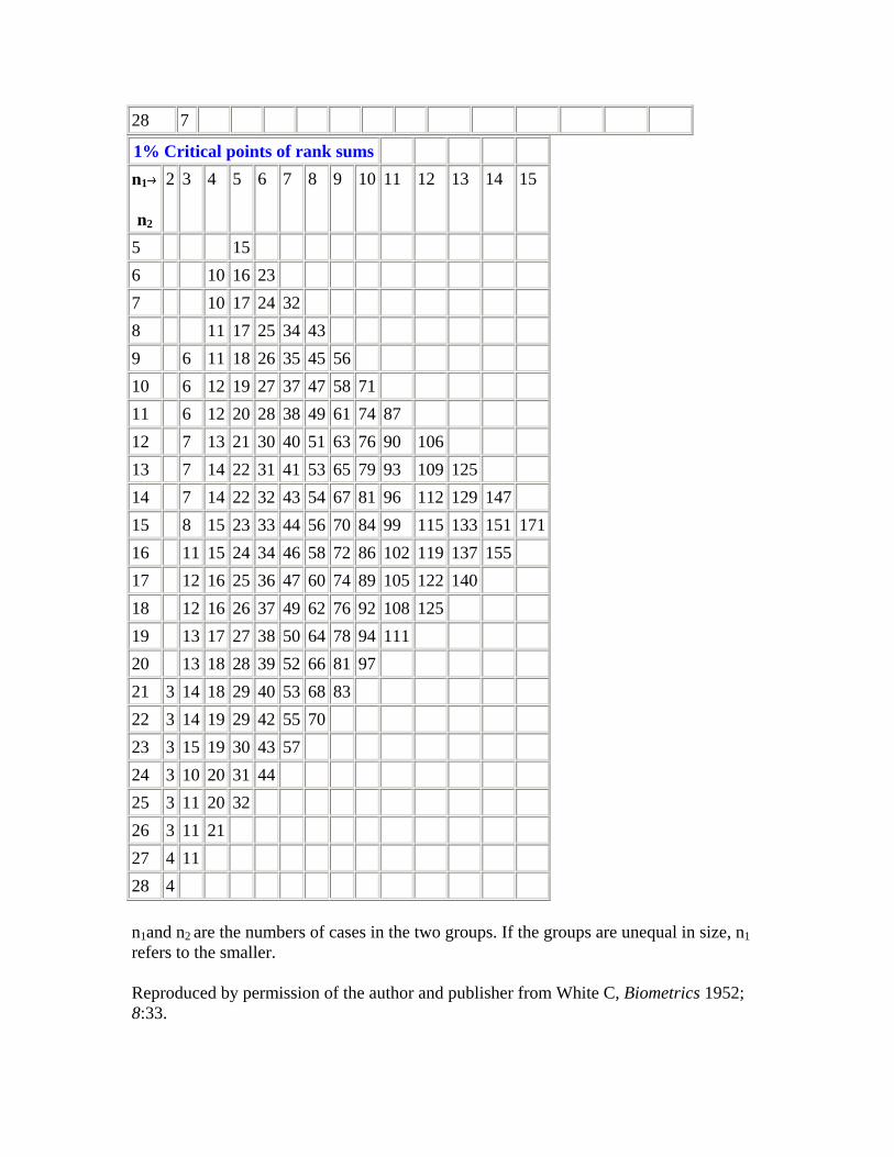
28 7

1% Critical points of rank sums n1

n2

2 3 4 5 6 7 8 9 10 11 12 13 14 15

5 15 6 10 16 23 7 10 17 24 32 8 11 17 25 34 43 9 6 11 18 26 35 45 56 10 6 12 19 27 37 47 58 71 11 6 12 20 28 38 49 61 74 87 12 7 13 21 30 40 51 63 76 90 106 13 7 14 22 31 41 53 65 79 93 109 125 14 7 14 22 32 43 54 67 81 96 112 129 147 15 8 15 23 33 44 56 70 84 99 115 133 151 17116 11 15 24 34 46 58 72 86 102 119 137 155 17 12 16 25 36 47 60 74 89 105 122 140 18 12 16 26 37 49 62 76 92 108 125 19 13 17 27 38 50 64 78 94 111 20 13 18 28 39 52 66 81 97 21 3 14 18 29 40 53 68 83 22 3 14 19 29 42 55 70 23 3 15 19 30 43 57 24 3 10 20 31 44 25 3 11 20 32 26 3 11 21 27 4 11 28 4

n1and n2 are the numbers of cases in the two groups. If the groups are unequal in size, n1 refers to the smaller.

Reproduced by permission of the author and publisher from White C, Biometrics 1952; 8:33.

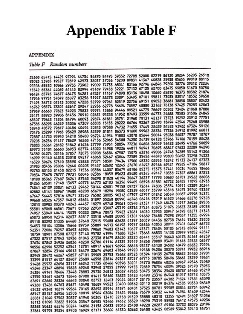
Appendix Table F

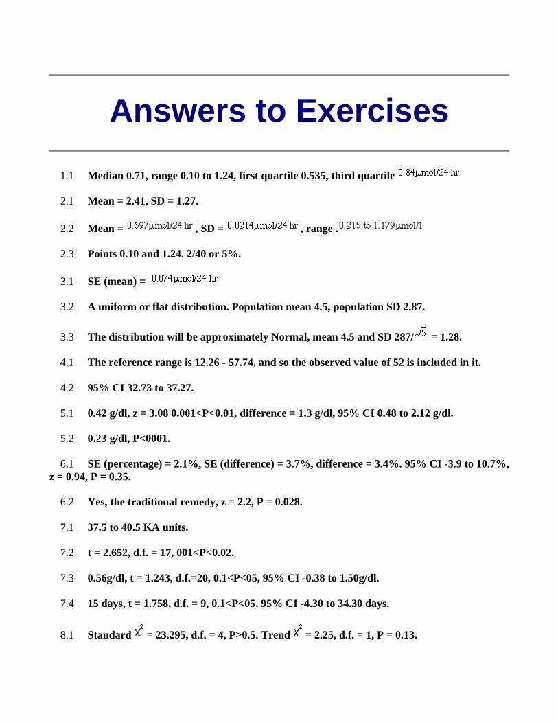
Answers to Exercises

1.1 Median 0.71, range 0.10 to 1.24, first quartile 0.535, third quartile

2.1 Mean = 2.41, SD = 1.27.

2.2 Mean = , SD = , range .

2.3 Points 0.10 and 1.24. 2/40 or 5%.

3.1 SE (mean) =

3.2 A uniform or flat distribution. Population mean 4.5, population SD 2.87.

3.3 The distribution will be approximately Normal, mean 4.5 and SD 287/ = 1.28.

4.1 The reference range is 12.26 - 57.74, and so the observed value of 52 is included in it.

4.2 95% CI 32.73 to 37.27.

5.1 0.42 g/dl, z = 3.08 0.001<P<0.01, difference = 1.3 g/dl, 95% CI 0.48 to 2.12 g/dl.

5.2 0.23 g/dl, P<0001.

6.1 SE (percentage) = 2.1%, SE (difference) = 3.7%, difference = 3.4%. 95% CI -3.9 to 10.7%, z = 0.94, P = 0.35.

6.2 Yes, the traditional remedy, z = 2.2, P = 0.028.

7.1 37.5 to 40.5 KA units.

7.2 t = 2.652, d.f. = 17, 001<P<0.02.

7.3 0.56g/dl, t = 1.243, d.f.=20, 0.1<P<05, 95% CI -0.38 to 1.50g/dl.

7.4 15 days, t = 1.758, d.f. = 9, 0.1<P<05, 95% CI -4.30 to 34.30 days.

8.1 Standard = 23.295, d.f. = 4, P>0.5. Trend = 2.25, d.f. = 1, P = 0.13.

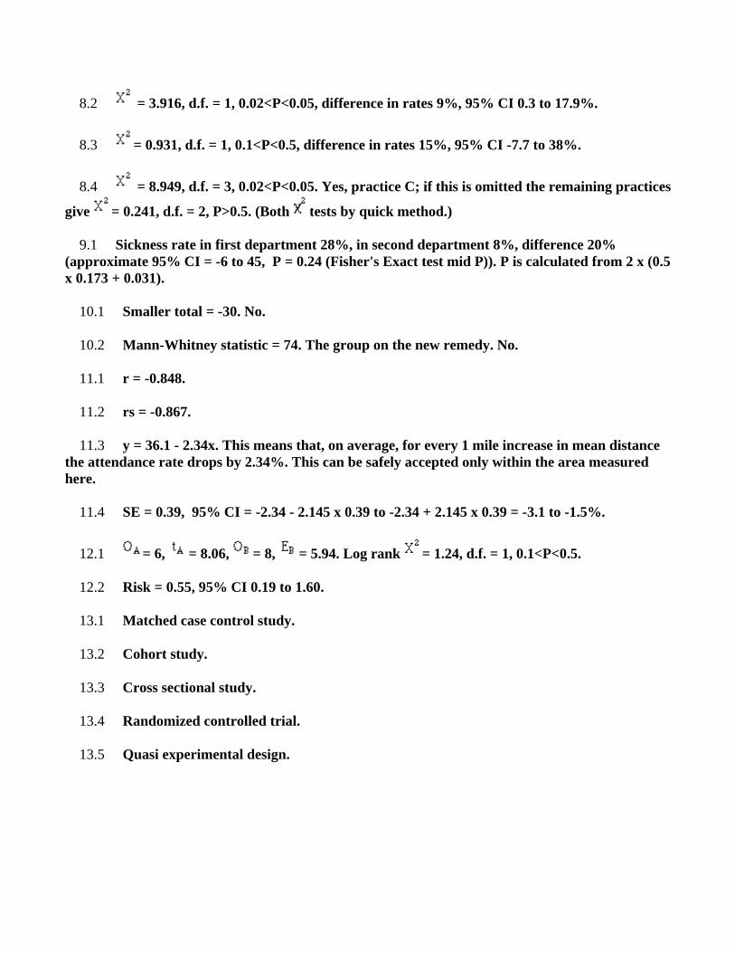
8.2 = 3.916, d.f. = 1, 0.02<P<0.05, difference in rates 9%, 95% CI 0.3 to 17.9%.

8.3 = 0.931, d.f. = 1, 0.1<P<0.5, difference in rates 15%, 95% CI -7.7 to 38%.

8.4 = 8.949, d.f. = 3, 0.02<P<0.05. Yes, practice C; if this is omitted the remaining practices

give = 0.241, d.f. = 2, P>0.5. (Both tests by quick method.)

9.1 Sickness rate in first department 28%, in second department 8%, difference 20% (approximate 95% CI = -6 to 45, P = 0.24 (Fisher's Exact test mid P)). P is calculated from 2 x (0.5 x 0.173 + 0.031).

10.1 Smaller total = -30. No.

10.2 Mann-Whitney statistic = 74. The group on the new remedy. No.

11.1 r = -0.848.

11.2 rs = -0.867.

11.3 y = 36.1 - 2.34x. This means that, on average, for every 1 mile increase in mean distance the attendance rate drops by 2.34%. This can be safely accepted only within the area measured here.

11.4 SE = 0.39, 95% CI = -2.34 - 2.145 x 0.39 to -2.34 + 2.145 x 0.39 = -3.1 to -1.5%.

12.1 = 6, = 8.06, = 8, = 5.94. Log rank = 1.24, d.f. = 1, 0.1<P<0.5.

12.2 Risk = 0.55, 95% CI 0.19 to 1.60.

13.1 Matched case control study.

13.2 Cohort study.

13.3 Cross sectional study.

13.4 Randomized controlled trial.

13.5 Quasi experimental design.

Glossary of Statistical Terms

A B C D E F G H I J K L M N O P Q R S T U V W X Y Z

A Age Distribution The frequency of different ages or age groups in a given population. The distribution may refer to either how many or what proportion of the group. The population is usually patients with a specific disease but the concept is not restricted to humans and is not restricted to medicine.

Age Factors Age as a constituent element or influence contributing to the production of a result. It may be applicable to the cause or the effect of a circumstance. It is used with human or animal concepts but should be differentiated from AGING, a physiological process, and time factors which refers only to the passage of time.

Alternative Hypothesis In hypothesis testing, a null hypothesis (typically, that there is no effect) is compared with an alternative hypothesis (typically, that there is an effect, or that there is an effect of a particular sign). For example, in evaluating whether a new cancer remedy works, the null hypothesis typically would be that the remedy does not work, while the alternative hypothesis would be that the remedy does work. When the data are sufficiently improbable under the assumption that the null hypothesis is true, the null hypothesis is rejected in favor of the alternative hypothesis. (This does not imply that the data are probable under the assumption that the alternative hypothesis is true, nor that the null hypothesis is false, nor that the alternative hypothesis is true.)

Analysis of Variance (ANOVA) An analytical method that compares the means of groups by analyzing each group's contribution to the overall uncertainty of the data, the variance. Arachnid Vectors Members of the class Arachnida, especially spiders, scorpions, mites, and ticks, which transmit infective organisms from one host to another or from an inanimate reservoir to an animate host.

Area Under Curve (AUC) A statistical means of summarizing information from a series of measurements on one individual. It is frequently used in clinical pharmacology where the AUC

from serum levels can be interpreted as the total uptake of whatever has been administered. As a plot of the concentration of a drug against time, after a single dose of medicine, producing a standard shape curve, it is a means of comparing the bioavailability of the same drug made by different companies.

Arthropod Vectors Arthropods, other than insects and arachnids, which transmit infective organisms from one host to another or from an inanimate reservoir to an animate host.

Association Two variables are associated if some of the variability of one can be accounted for by the other. In a scatterplot of the two variables, if the scatter in the values of the variable plotted on the vertical axis is smaller in narrow ranges of the variable plotted on the horizontal axis (i.e., in vertical "slices") than it is overall, the two variables are associated. The correlation coefficient is a measure of linear association, which is a special case of association in which large values of one variable tend to occur with large values of the other, and small values of one tend to occur with small values of the other (positive association), or in which large values of one tend to occur with small values of the other, and vice versa (negative association).

Average Average usually denotes the arithmetic mean, but it can also denote the median, the mode, the geometric mean, and weighted means, among other things. Axioms of Probability There are three axioms of probability: (1) Chances are always at least zero. (2) The chance that something happens is 100%. (3) If two events cannot both occur at the same time (if they are disjoint or mutually exclusive), the chance that either one occurs is the sum of the chances that each occurs. For example, consider an experiment that consists of tossing a coin once. The first axiom says that the chance that the coin lands heads, for instance, must be at least zero. The second axiom says that the chance that the coin either lands heads or lands tails or lands on its edge or doesn't land at all is 100%. The third axiom says that the chance that the coin either lands heads or lands tails is the sum of the chance that the coin lands heads and the chance that the coin lands tails, because both cannot occur in the same coin toss. All other mathematical facts about probability can be derived from these three axioms. For example, it is true that the chance that an event does not occur is (100% - the chance that the event occurs). This is a consequence of the second and third axioms.

top

B Balance The condition in a study in which all subgroups being analyzed have equal numbers of patients.

Bias A measurement procedure or estimator is said to be biased if, on the average, it gives an answer that differs from the truth. The bias is the average (expected) difference between the measurement and the truth. For example, if you get on the scale with clothes on, that

biases the measurement to be larger than your true weight (this would be a positive bias). The design of an experiment or of a survey can also lead to bias. Bias can be deliberate, but it is not necessarily so.

Bimodal Having two modes. Binomial Distribution A random variable has a binomial distribution (with parameters n and p) if it is the number of "successes" in a fixed number n of independent random trials, all of which have the same probability p of resulting in "success." Under these assumptions, the probability of k successes (and n-k failures) is nCk pk(1-p)n-k, where nCk is the number of combinations of n objects taken k at a time: nCk = n!/(k!(n-k)!). The expected value of a random variable with the Binomial distribution is n×p, and the standard error of a random variable with the Binomial distribution is (n×p×(1 - p))½. Bivariate Having or having to do with two variables. For example, bivariate data are data where we have two measurements of each "individual." These measurements might be the heights and weights of a group of people (an "individual" is a person), the heights of fathers and sons (an "individual" is a father-son pair), the pressure and temperature of a fixed volume of gas (an "individual" is the volume of gas under a certain set of experimental conditions), etc. Scatterplots, the correlation coefficient, and regression make sense for bivariate data but not univariate data. C.f. univariate. Blind, Blind Experiment In a blind experiment, the subjects do not know whether they are in the treatment group or the control group. In order to have a blind experiment with human subjects, it is usually necessary to administer a placebo to the control group.

Binomial Distribution The probability distribution associated with two mutually exclusive outcomes; used to model cumulative incidence rates and prevalence rates. The Bernoulli distribution is a special case of binomial distribution.

Biometry The use of statistical methods to analyze biological observations and phenomena.

Birth Certificates Official certifications by a physician recording the individual's birth date, place of birth, parentage and other required identifying data which are filed with the local registrar of vital statistics.

Birth Order The sequence in which children are born into the family.

Birth Rate The number of births in a given population per year or other unit of time.

Bootstrap estimate of Standard Error The name for this idea comes from the idiom "to pull oneself up by one's bootstraps," which connotes getting out of a hole without anything to stand on. The idea of the bootstrap is to assume, for the purposes of estimating uncertainties, that the sample is the population, then use the SE for sampling from the sample to estimate the SE of sampling from the population. For sampling from a box of numbers, the SD of the sample is

the bootstrap estimate of the SD of the box from which the sample is drawn. For sample percentages, this takes a particularly simple form: the SE of the sample percentage of n draws from a box, with replacement, is SD(box)/n½, where for a box that contains only zeros and ones, SD(box) = ((fraction of ones in box)×(fraction of zeros in box) )½. The bootstrap estimate of the SE of the sample percentage consists of estimating SD(box) by ((fraction of ones in sample)×(fraction of zeros in sample))½. When the sample size is large, this approximation is likely to be good.

top

C Catchment Area (Health) A geographic area defined and served by a health program or institution.

Causality The relating of causes to the effects they produce. Causes are termed necessary when they must always precede an effect and sufficient when they initiate or produce an effect. Any of several factors may be associated with the potential disease causation or outcome, including predisposing factors, enabling factors, precipitating factors, reinforcing factors, and risk factors.

Cause of Death Factors which produce cessation of all vital bodily functions. They can be analyzed from an epidemiologic viewpoint.

Censuses Enumerations of populations usually recording identities of all persons in every place of residence with age or date of birth, sex, occupation, national origin, language, marital status, income, relation to head of household, information on the dwelling place, education, literacy, health-related data (e.g., permanent disability), etc.

Chi-Square Distribution A distribution in which a variable is distributed like the sum of the the squares of any given independent random variable, each of which has a normal distribution with mean of zero and variance of one. The chi-square test is a statistical test based on comparison of a test statistic to a chi-square distribution. The oldest of these tests are used to detect whether two or more population distributions differ from one another.

Chi-Square Methods A group of qualitative variable techniques whose results are compared to values found in a theoretical Chi-square distribution table.

Clinical Trials Pre-planned studies of the safety, efficacy, or optimum dosage schedule (if appropriate) of one or more diagnostic, therapeutic, or prophylactic drugs, devices, or techniques selected according to predetermined criteria of eligibility and observed for predefined evidence of favorable and unfavorable effects. This concept includes clinical trials conducted both in the U.S. and in other countries.

Clinical Trials, Phase I Studies performed to evaluate the safety of diagnostic, therapeutic, or prophylactic drugs, devices, or techniques in healthy subjects and to determine the safe dosage range (if appropriate). These tests also are used to determine pharmacologic and pharmacokinetic properties (toxicity, metabolism, absorption, elimination, and preferred route of administration). They involve a small number of persons and usually last about 1 year. This concept includes phase I studies conducted both in the U.S. and in other countries.

Clinical Trials, Phase II Studies that are usually controlled to assess the effectiveness and dosage (if appropriate) of diagnostic, therapeutic, or prophylactic drugs, devices, or techniques. These studies are performed on several hundred volunteers, including a limited number of patients with the target disease or disorder, and last about two years. This concept includes phase II studies conducted in both the U.S. and in other countries.

Clinical Trials, Phase III Comparative studies to verify the effectiveness of diagnostic, therapeutic, or prophylactic drugs, devices, or techniques determined in phase II studies. During these trials, patients are monitored closely by physicians to identify any adverse reactions from long-term use. These studies are performed on groups of patients large enough to identify clinically significant responses and usually last about three years. This concept includes phase III studies conducted in both the U.S. and in other countries.

Clinical Trials, Phase IV Planned post-marketing studies of diagnostic, therapeutic, or prophylactic drugs, devices, or techniques that have been approved for general sale. These studies are often conducted to obtain additional data about the safety and efficacy of a product. This concept includes phase IV studies conducted in both the U.S. and in other countries.

Cochran-Mantel-Haenzel Method A Chi-square method that permits statistical comparison of odds ratios across subgroups and also allows differences in those ratios to be adjusted.

Controlled Clinical Trials Clinical trials involving one or more test treatments, at least one control treatment, specified outcome measures for evaluating the studied intervention, and a bias-free method for assigning patients to the test treatment. The treatment may be drugs, devices, or procedures studied for diagnostic, therapeutic, or prophylactic effectiveness. Control measures include placebos, active medicines, no-treatment, dosage forms and regimens, historical comparisons, etc. When randomization using mathematical techniques, such as the use of a random numbers table, is employed to assign patients to test or control treatments, the trials are characterized as randomized controlled trials. However, trials employing treatment allocation methods such as coin flips, odd-even numbers, patient social security numbers, days of the week, medical record numbers, or other such pseudo- or quasi-random processes, are simply designated as controlled clinical trials.

Correlation Coefficient In linear regression, a measure of the closeness of data points to the best-fit line. It can assume a value between -1 and +1; the nearer the value to either -1 or +1, the nearer are the points to the line.

Cox Regression Method An analytical method in which event data for each group under comparison are transformed to fit a linear model. Models for each group are then compared to determine whether they are equal. This method assumes that hazard rates for each group are at least proportional to each other.

Cluster Analysis A set of statistical methods used to group variables or observations into strongly inter-related subgroups. In epidemiology, it may be used to analyze a closely grouped series of events or cases of disease or other health-related phenomenon with well-defined distribution patterns in relation to time or place or both.

Confidence Intervals A range of values for a variable of interest, e.g., a rate, constructed so that this range has a specified probability of including the true value of the variable.

Confounding Factors (Epidemiology) Factors that can cause or prevent the outcome of interest, are not intermediate variables, and are not associated with the factor(s) under investigation. They give rise to situations in which the effects of two processes are not separated, or the contribution of causal factors cannot be separated, or the measure of the effect of exposure or risk is distorted because of its association with other factors influencing the outcome of the study.

Comorbidity The presence of co-existing or additional diseases with reference to an initial diagnosis or with reference to the index condition that is the subject of study. Comorbidity may affect the ability of affected individuals to function and also their survival; it may be used as a prognostic indicator for length of hospital stay, cost factors, and outcome or survival.

Cross Sectional Study In survey research, a study in which data are obtained only once. Contrast with longitudinal studies in which a panel of individuals is interviewed repeatedly over a period of time. Note that a cross sectional study can ask questions about previous periods of time, though. Categorical Variable A variable whose value ranges over categories, such as {red, green, blue}, {male, female}, {Arizona, California, Montana, New York}, {short, tall}, {Asian, African-American, Caucasian, Hispanic, Native American, Polynesian}, {straight, curly}, etc. Some categorical variables are ordinal. The distinction between categorical variables and qualitative variables is a bit blurry. C.f. quantitative variable. Causation, causal relation Two variables are causally related if changes in the value of one cause the other to change. For example, if one heats a rigid container filled with a gas, that causes the pressure of the gas in the container to increase. Two variables can be associated without having any causal relation, and even if two variables have a causal relation, their correlation can be small or zero. Central Limit Theorem The central limit theorem states that the probability histograms of the sample mean and sample sum of n draws with replacement from a box of labeled tickets converge to a normal curve as the sample size n grows, in the following sense: As n grows, the area of the probability histogram for any range of values approaches the area under the

normal curve for the same range of values, converted to standard units. See also the normal approximation. Certain Event An event is certain if its probability is 100%. Even if an event is certain, it might not occur. However, by the complement rule, the chance that it does not occur is 0%. Chance variation, chance error A random variable can be decomposed into a sum of its expected value and chance variation around its expected value. The expected value of the chance variation is zero; the standard error of the chance variation is the same as the standard error of the random variable---the size of a "typical" difference between the random variable and its expected value. See also sampling error. Chebychev's Inequality For lists: For every number k>0, the fraction of elements in a list that are k SD's or further from the arithmetic mean of the list is at most 1/k2. For random variables: For every number k>0, the probability that a random variable X is k SEs or further from its expected value is at most 1/k2. Chi-square curve The chi-square curve is a family of curves that depend on a parameter called degrees of freedom (d.f.). The chi-square curve is an approximation to the probability histogram of the chi-square statistic for multinomial model if the expected number of outcomes in each category is large. The chi-square curve is positive, and its total area is 100%, so we can think of it as the probability histogram of a random variable. The balance point of the curve is d.f., so the expected value of the corresponding random variable would equal d.f.. The standard error of the corresponding random variable would be (2×d.f.)½. As d.f. grows, the shape of the chi-square curve approaches the shape of the normal curve. Chi-square Statistic The chi-square statistic is used to measure the agreement between categorical data and a multinomial model that predicts the relative frequency of outcomes in each possible category. Suppose there are n independent trials, each of which can result in one of k possible outcomes. Suppose that in each trial, the probability that outcome i occurs is pi, for i = 1, 2, . . . , k, and that these probabilities are the same in every trial. The expected number of times outcome 1 occurs in the n trials is n×p1; more generally, the expected number of times outcome i occurs is expectedi = n×pi. If the model is correct, we would expect the n trials to result in outcome i about n×pi times, give or take a bit. Let observedi denote the number of times an outcome of type i occurs in the n trials, for i = 1, 2, . . . , k. The chi-squared statistic summarizes the discrepancies between the expected number of times each outcome occurs (assuming that the model is true) and the observed number of times each outcome occurs, by summing the squares of the discrepancies, normalized by the expected numbers, over all the categories:

chi-squared =

(observed1 - expected1)2/expected1 + (observed2 - expected2)2/expected2 + . . . + (observedk - expectedk)2/expectedk.

As the sample size n increases, if the model is correct, the sampling distribution of the chi-squared statistic is approximated increasingly well by the chi-squared curve with (#categories -

1) = k - 1 degrees of freedom (d.f.), in the sense that the chance that the chi-squared statistic is in any given range grows closer and closer to the area under the Chi-Squared curve over the same range.

Class Boundary A point that is the left endpoint of one class interval, and the right endpoint of another class interval. Class Interval In plotting a histogram, one starts by dividing the range of values into a set of non-overlapping intervals, called class intervals, in such a way that every datum is contained in some class interval. See the related entries class boundary and endpoint convention. Cluster Sample In a cluster sample, the sampling unit is a collection of population units, not single population units. For example, techniques for adjusting the U.S. census start with a sample of geographic blocks, then (try to) enumerate all inhabitants of the blocks in the sample to obtain a sample of people. This is an example of a cluster sample. (The blocks are chosen separately from different strata, so the overall design is a stratified cluster sample.) Combinations The number of combinations of n things taken k at a time is the number of ways of picking a subset of k of the n things, without replacement, and without regard to the order in which the elements of the subset are picked. The number of such combinations is nCk = n!/(k!(n-k)!), where k! (pronounced "k factorial") is k×(k-1)×(k-2)× · · · × 1. The numbers nCk are also called the Binomial coefficients. From a set that has n elements one can form a total of 2n subsets of all sizes. For example, from the set {a, b, c}, which has 3 elements, one can form the 23 = 8 subsets {}, {a}, {b}, {c}, {a,b}, {a,c}, {b,c}, {a,b,c}. Because the number of subsets with k elements one can form from a set with n elements is nCk, and the total number of subsets of a set is the sum of the numbers of possible subsets of each size, it follows that nC0+nC1+nC2+ . . . +nCn = 2n. The calculator has a button (nCm) that lets you compute the number of combinations of m things chosen from a set of n things. To use the button, first type the value of n, then push the nCm button, then type the value of m, then press the "=" button. Complement The complement of a subset of a given set is the collection of all elements of the set that are not elements of the subset. Complement rule The probability of the complement of an event is 100% minus the probability of the event: P(Ac) = 100% - P(A). Conditional Probability Suppose we are interested in the probability that some event A occurs, and we learn that the event B occurred. How should we update the probability of A to reflect this new knowledge? This is what the conditional probability does: it says how the additional knowledge that B occurred should affect the probability that A occurred quantitatively. For example, suppose that A and B are mutually exclusive. Then if B occurred, A did not, so the conditional probability that A occurred given that B occurred is zero. At the other extreme, suppose that B is a subset of A, so that A must occur whenever B does. Then if we learn that B occurred, A must have occurred too, so the conditional probability that A occurred given that B occurred is 100%. For in-between cases, where A and B intersect, but B is not a subset of A, the conditional probability of A given B is a number between zero and

100%. Basically, one "restricts" the outcome space S to consider only the part of S that is in B, because we know that B occurred. For A to have happened given that B happened requires that AB happened, so we are interested in the event AB. To have a legitimate probability requires that P(S) = 100%, so if we are restricting the outcome space to B, we need to divide by the probability of B to make the probability of this new S be 100%. On this scale, the probability that AB happened is P(AB)/P(B). This is the definition of the conditional probability of A given B, provided P(B) is not zero (division by zero is undefined). Note that the special cases AB = {} (A and B are mutually exclusive) and AB = B (B is a subset of A) agree with our intuition as described at the top of this paragraph. Conditional probabilities satisfy the axioms of probability, just as ordinary probabilities do. Confidence Interval A confidence interval for a parameter is a random interval constructed from data in such a way that the probability that the interval contains the true value of the parameter can be specified before the data are collected. Confidence Level The confidence level of a confidence interval is the chance that the interval that will result once data are collected will contain the corresponding parameter. If one computes confidence intervals again and again from independent data, the long-term limit of the fraction of intervals that contain the parameter is the confidence level. Confounding When the differences between the treatment and control groups other than the treatment produce differences in response that are not distinguishable from the effect of the treatment, those differences between the groups are said to be confounded with the effect of the treatment (if any). For example, prominent statisticians questioned whether differences between individuals that led some to smoke and others not to (rather than the act of smoking itself) were responsible for the observed difference in the frequencies with which smokers and non-smokers contract various illnesses. If that were the case, those factors would be confounded with the effect of smoking. Confounding is quite likely to affect observational studies and experiments that are not randomized. Confounding tends to be decreased by randomization. See also Simpson's Paradox. Continuity Correction In using the normal approximation to the binomial probability histogram, one can get more accurate answers by finding the area under the normal curve corresponding to half-integers, transformed to standard units. This is clearest if we are seeking the chance of a particular number of successes. For example, suppose we seek to approximate the chance of 10 successes in 25 independent trials, each with probability p = 40% of success. The number of successes in this scenario has a binomial distribution with parameters n = 25 and p = 40%. The expected number of successes is np = 10, and the standard error is (np(1-p))½ = 6½ = 2.45. If we consider the area under the normal curve at the point 10 successes, transformed to standard units, we get zero: the area under a point is always zero. We get a better approximation by considering 10 successes to be the range from 9 1/2 to 10 1/2 successes. The only possible number of successes between 9 1/2 and 10 1/2 is 10, so this is exactly right for the binomial distribution. Because the normal curve is continuous and a binomial random variable is discrete, we need to "smear out" the binomial probability over an appropriate range. The lower endpoint of the range, 9 1/2 successes, is (9.5 - 10)/2.45 = -0.20 standard units. The upper endpoint of the range, 10 1/2 successes, is (10.5 - 10)/2.45

= +0.20 standard units. The area under the normal curve between -0.20 and +0.20 is about 15.8%. The true binomial probability is 25C10×(0.4)10×(0.6)15 = 16%. In a similar way, if we seek the normal approximation to the probability that a binomial random variable is in the range from i successes to k successes, inclusive, we should find the area under the normal curve from i-1/2 to k+1/2 successes, transformed to standard units. If we seek the probability of more than i successes and fewer than k successes, we should find the area under the normal curve corresponding to the range i+1/2 to k-1/2 successes, transformed to standard units. If we seek the probability of more than i but no more than k successes, we should find the area under the normal curve corresponding to the range i+1/2 to k+1/2 successes, transformed to standard units. If we seek the probability of at least i but fewer than k successes, we should find the area under the normal curve corresponding to the range i-1/2 to k-1/2 successes, transformed to standard units. Including or excluding the half-integer ranges at the ends of the interval in this manner is called the continuity correction. Continuous Variable A quantitative variable is continuous if its set of possible values is uncountable. Examples include temperature, exact height, exact age (including parts of a second). In practice, one can never measure a continuous variable to infinite precision, so continuous variables are sometimes approximated by discrete variables. A random variable X is also called continuous if its set of possible values is uncountable, and the chance that it takes any particular value is zero (in symbols, if P(X = x) = 0 for every real number x). A random variable is continuous if and only if its cumulative probability distribution function is a continuous function (a function with no jumps). Contrapositive If p and q are two logical propositions, then the contrapositive of the proposition (p IMPLIES q) is the proposition ((NOT q) IMPLIES (NOT p) ). The contrapositive is logically equivalent to the original proposition. Control There are at least three senses of "control" in statistics: a member of the control group, to whom no treatment is given; a controlled experiment, and to control for a possible confounding variable. Controlled experiment An experiment that uses the method of comparison to evaluate the effect of a treatment by comparing treated subjects with a control group, who do not receive the treatment. Controlled, randomized experiment A controlled experiment in which the assignment of subjects to the treatment group or control group is done at random, for example, by tossing a coin. Control for a variable To control for a variable is to try to separate its effect from the treatment effect, so it will not confound with the treatment. There are many methods that try to control for variables. Some are based on matching individuals between treatment and control; others use assumptions about the nature of the effects of the variables to try to model the effect mathematically, for example, using regression. Control group The subjects in a controlled experiment who do not receive the treatment.

Convenience Sample A sample drawn because of its convenience; not a probability sample. For example, I might take a sample of opinions in Columbus (where I live) by just asking my 10 nearest neighbors. That would be a sample of convenience, and would be unlikely to be representative of all of Columbus. Samples of convenience are not typically representative, and it is not typically possible to quantify how unrepresentative results based on samples of convenience will be. Converge, convergence A sequence of numbers x1, x2, x3 . . . converges if there is a number x such that for any number E>0, there is a number k (which can depend on E) such that |xj - x| < E whenever j > k. If such a number x exists, it is called the limit of the sequence x1, x2, x3 . . . . Convergence in probability A sequence of random variables X1, X2, X3 . . . converges in probability if there is a random variable X such that for any number E>0, the sequence of numbers P(|X1 - X| < e), P(|X2 - X| < e), P(|X3 - X| < e), . . . converges to 100%. Converse If p and q are two logical propositions, then the converse of the proposition (p IMPLIES q) is the proposition (q IMPLIES p). Correlation A measure of linear association between two (ordered) lists. Two variables can be strongly correlated without having any causal relationship, and two variables can have a causal relationship and yet be uncorrelated. Correlation coefficient The correlation coefficient r is a measure of how nearly a scatterplot falls on a straight line. The correlation coefficient is always between -1 and +1. To compute the correlation coefficient of a list of pairs of measurements (X,Y), first transform X and Y individually into standard units. Multiply corresponding elements of the transformed pairs to get a single list of numbers. The correlation coefficient is the mean of that list of products. Countable Set A set is countable if its elements can be put in one-to-one correspondence with a subset of the integers. For example, the sets {0, 1, 7, -3}, {red, green, blue}, { . . . ,-2, -1, 0, 1, 2, . . . }, {straight, curly}, and the set of all fractions, are countable. If a set is not countable, it is uncountable. The set of all real numbers is uncountable. Cover A confidence interval is said to cover if the interval contains the true value of the parameter. Before the data are collected, the chance that the confidence interval will contain the parameter value is the coverage probability, which equals the confidence level after the data are collected and the confidence interval is actually computed. Coverage probability The coverage probability of a procedure for making confidence intervals is the chance that the procedure produces an interval that covers the truth. Critical value The critical value in an hypothesis test is the value of the test statistic beyond which we would reject the null hypothesis. The critical value is set so that the probability that

the test statistic is beyond the critical value is at most equal to the significance level if the null hypothesis be true. Cross-sectional study A cross-sectional study compares different individuals to each other at the same time--it looks at a cross-section of a population. The differences between those individuals can confound with the effect being explored. For example, in trying to determine the effect of age on sexual promiscuity, a cross-sectional study would be likely to confound the effect of age with the effect of the mores the subjects were taught as children: the older individuals were probably raised with a very different attitude towards promiscuity than the younger subjects. Thus it would be imprudent to attribute differences in promiscuity to the aging process. C.f. longitudinal study. Cumulative Probability Distribution Function (cdf) The cumulative distribution function of a random variable is the chance that the random variable is less than or equal to x, as a function of x. In symbols, if F is the cdf of the random variable X, then F(x) = P( X <= x). The cumulative distribution function must tend to zero as x approaches minus infinity, and must tend to unity as x approaches infinity. It is a positive function, and increases monotonically: if y > x, then F(y) >= F(x). The cumulative distribution function completely characterizes the probability distribution of a random variable.

top

D Data Collection Systematic gathering of data for a particular purpose from various sources, including questionnaires, interviews, observation, existing records, and electronic devices. The process is usually preliminary to statistical analysis of the data.

Data Interpretation, Statistical Application of statistical procedures to analyze specific observed or assumed facts from a particular study.

Death Certificates Official records of individual deaths including the cause of death certified by a physician, and any other required identifying information.

Demography Statistical interpretation and description of a population with reference to distribution, composition, or structure.

Density, Density Scale The vertical axis of a histogram has units of percent per unit of the horizontal axis. This is called a density scale; it measures how "dense" the observations are in each bin. See also probability density.

Dental Health Surveys A systematic collection of factual data pertaining to dental or oral health and disease in a human population within a given geographic area.

Dependent Events, Dependent Random Variables Two events or random variables are dependent if they are not independent. Dependent Variable In regression, the variable whose values are supposed to be explained by changes in the other variable (the the independent or explanatory variable). Usually one regresses the dependent variable on the independent variable. Deviation A deviation is the difference between a datum and some reference value, typically the mean of the data. In computing the SD, one finds the rms of the deviations from the mean, the differences between the individual data and the mean of the data.

Diet Surveys Systematic collections of factual data pertaining to the diet of a human population within a given geographic area.

Discrete Variable A quantitative variable whose set of possible values is countable. Typical examples of discrete variables are variables whose possible values are a subset of the integers, such as Social Security numbers, the number of people in a family, ages rounded to the nearest year, etc. Discrete variables are "chunky." C.f. continuous variable. A discrete random variable is one whose set of possible values is countable. A random variable is discrete if and only if its cumulative probability distribution function is a stair-step function; i.e., if it is piecewise constant and only increases by jumps.

Discriminant Analysis A statistical analytic technique used with discrete dependent variables, concerned with separating sets of observed values and allocating new values. It is sometimes used instead of regression analysis.

Disease-Free Survival Period after successful treatment in which there is no appearance of the symptoms or effects of the disease.

Disease Notification Notification or reporting by a physician or other health care provider of the occurrence of specified contagious diseases such as tuberculosis and HIV infections to designated public health agencies. The United States system of reporting notifiable diseases evolved from the Quarantine Act of 1878, which authorized the US Public Health Service to collect morbidity data on cholera, smallpox, and yellow fever; each state in the U.S. (as well as the USAF) has its own list of notifiable diseases and depends largely on reporting by the individual health care provider.

Disease Outbreaks Sudden increase in the incidence of a disease. The concept includes epidemics.

Disease Transmission The transmission of infectious disease or pathogens. When transmission is within the same species, the mode can be horizontal or vertical.

Disease Transmission, Horizontal The transmission of infectious disease or pathogens from one individual to another in the same generation.

Disease Transmission, Patient-to-Professional The transmission of infectious disease or pathogens from patients to health professionals or health care workers. It includes transmission via direct or indirect exposure to bacterial, fungal, parasitic, or viral agents.

Disease Transmission, Professional-to-Patient The transmission of infectious disease or pathogens from health professional or health care worker to patients. It includes transmission via direct or indirect exposure to bacterial, fungal, parasitic, or viral agents

Disease Transmission, Vertical The transmission of infectious disease or pathogens from one generation to another. It includes transmission in utero or intrapartum by exposure to blood and secretions, and postpartum exposure via breastfeeding.

Disease Vectors Invertebrates or non-human vertebrates which transmit infective organisms from one host to another.

Disjoint or Mutually Exclusive Events Two events are disjoint or mutually exclusive if the occurrence of one is incompatible with the occurrence of the other; that is, if they can't both happen at once (if they have no outcome in common). Equivalently, two events are disjoint if their intersection is the empty set. Distribution The distribution of a set of numerical data is how their values are distributed over the real numbers. It is completely characterized by the empirical distribution function. Similarly, the probability distribution of a random variable is completely characterized by its probability distribution function. Sometimes the word "distribution" is used as a synonym for the empirical distribution function or the probability distribution function. Distribution Function, Empirical The empirical (cumulative) distribution function of a set of numerical data is, for each real value of x, the fraction of observations that are less than or equal to x. A plot of the empirical distribution function is an uneven set of stairs. The width of the stairs is the spacing between adjacent data; the height of the stairs depends on how many data have exactly the same value. The distribution function is zero for small enough (negative) values of x, and is unity for large enough values of x. It increases monotonically: if y > x, the empirical distribution function evaluated at y is at least as large as the empirical distribution function evaluated at x.

Distribution (or Probability Distribution) A mathematical function characterized by constants, called parameters, that relate the values that a variable can assume to the probability that a particular value will occur.

Double-Blind, Double-Blind Experiment In a double-blind experiment, neither the subjects nor the people evaluating the subjects knows who is in the treatment group and who is in the control group. This mitigates the placebo effect and guards against conscious and unconscious prejudice for or against the treatment on the part of the evaluators.

Double-Blind Method A method of studying a drug or procedure in which both the subjects and investigators are kept unaware of who is actually getting which specific treatment.

top

E Ecological Correlation The correlation between averages of groups of individuals, instead of individuals. Ecological correlation can be misleading about the association of individuals. Effect Modifiers (Epidemiology) Factors that modify the effect of the putative causal factor(s) under study. Empirical Law of Averages The Empirical Law of Averages lies at the base of the frequency theory of probability. This law, which is, in fact, an assumption about how the world works, rather than a mathematical or physical law, states that if one repeats a random experiment over and over, independently and under "identical" conditions, the fraction of trials that result in a given outcome converges to a limit as the number of trials grows without bound. Empty Set The empty set, denoted {} or Ø, is the set that has no members. Endpoint Convention In plotting a histogram, one must decide whether to include a datum that lies at a class boundary with the class interval to the left or the right of the boundary. The rule for making this assignment is called an endpoint convention. The two standard endpoint conventions are (1) to include the left endpoint of all class intervals and exclude the right, except for the rightmost class interval, which includes both of its endpoints, and (2) to include the right endpoint of all class intervals and exclude the left, except for the leftmost interval, which includes both of its endpoints. Estimator An estimator is a rule for "guessing" the value of a population parameter based on a random sample from the population. An estimator is a random variable, because its value depends on which particular sample is obtained, which is random. A canonical example of an estimator is the sample mean, which is an estimator of the population mean. Event An event is a subset of outcome space. An event determined by a random variable is an event of the form A=(X is in A). When the random variable X is observed, that determines whether or not A occurs: if the value of X happens to be in A, A occurs; if not, A does not occur. Exhaustive A collection of events {A1, A2, A3, . . . } is exhaustive if at least one of them must occur; that is, if S = A1 U A2 U A3 U . . . where S is the outcome space. A collection of subsets exhausts another set if that set is contained in the ] union of the collection.

Expectation, Expected Value The expected value of a random variable is the long-term limiting average of its values in independent repeated experiments. The expected value of the random variable X is denoted EX or E(X). For a discrete random variable (one that has a countable number of possible values) the expected value is the weighted average of its possible values, where the weight assigned to each possible value is the chance that the random variable takes that value. One can think of the expected value of a random variable as the point at which its probability histogram would balance, if it were cut out of a uniform material. Taking the expected value is a linear operation: if X and Y are two random variables, the expected value of their sum is the sum of their expected values (E(X+Y) = E(X) + E(Y)), and the expected value of a constant a times a random variable X is the constant times the expected value of X (E(a×X ) = a× E(X)). Experiment What distinguishes an experiment from an observational study is that in an experiment, the experimenter decides who receives the treatment. Explanatory Variable In regression, the explanatory or independent variable is the one that is supposed to "explain" the other. For example, in examining crop yield versus quantity of fertilizer applied, the quantity of fertilizer would be the explanatory or independent variable, and the crop yield would be the dependent variable. In experiments, the explanatory variable is the one that is manipulated; the one that is observed is the dependent variable. Extrapolation See interpolation.

top

F Factor Analysis, Statistical A set of statistical methods for analyzing the correlations among several variables in order to estimate the number of fundamental dimensions that underlie the observed data and to describe and measure those dimensions. It is used frequently in the development of scoring systems for rating scales and questionnaires.

Factorial For an integer k that is greater than or equal to 1, k! (pronounced "k factorial") is k×(k-1)×(k-2)× . . . ×1. By convention, 0! = 1. There are k! ways of ordering k distinct objects. For example, 9! is the number of batting orders of 9 baseball players, and 52! is the number of different ways a standard deck of playing cards can be ordered. The calculator above has a button to compute the factorial of a number. To compute k!, first type the value of k, then press the button labeled "!". False Discovery Rate In testing a collection of hypotheses, the false discovery rate is the fraction of rejected null hypotheses that are rejected erroneously (the number of Type I errors

divided by the number of rejected null hypotheses), with the convention that if no hypothesis is rejected, the false discovery rate is zero.

Family Characteristics Size and composition of the family.

Fatal Outcome Death resulting from the presence of a disease in an individual, as shown by a single case report or a limited number of patients. This should be differentiated from death, the physiological cessation of life and from mortality, an epidemiological or statistical concept.

Finite Population Correction When sampling without replacement, as in a simple random sample, the SE of sample sums and sample means depends on the fraction of the population that is in the sample: the greater the fraction, the smaller the SE. Sampling with replacement is like sampling from an infinitely large population. The adjustment to the SE for sampling without replacement is called the finite population correction. The SE for sampling without replacement is smaller than the SE for sampling with replacement by the finite population correction factor ((N -n)/(N - 1))½. Note that for sample size n=1, there is no difference between sampling with and without replacement; the finite population correction is then unity. If the sample size is the entire population of N units, there is no variability in the result of sampling without replacement (every member of the population is in the sample exactly once), and the SE should be zero. This is indeed what the finite population correction gives (the numerator vanishes). Fisher's exact test (for the equality of two percentages) Consider two populations of zeros and ones. Let p1 be the proportion of ones in the first population, and let p2 be the proportion of ones in the second population. We would like to test the null hypothesis that p1 = p2 on the basis of a simple random sample from each population. Let n1 be the size of the sample from population 1, and let n2 be the size of the sample from population 2. Let G be the total number of ones in both samples. If the null hypothesis be true, the two samples are like one larger sample from a single population of zeros and ones. The allocation of ones between the two samples would be expected to be proportional to the relative sizes of the samples, but would have some chance variability. Conditional on G and the two sample sizes, under the null hypothesis, the tickets in the first sample are like a random sample of size n1 without replacement from a collection of N = n1 + n2 units of which G are labeled with ones. Thus, under the null hypothesis, the number of tickets labeled with ones in the first sample has (conditional on G) an hypergeometric distribution with parameters N, G, and n1. Fisher's exact test uses this distribution to set the ranges of observed values of the number of ones in the first sample for which we would reject the null hypothesis. Football-Shaped Scatterplot In a football-shaped scatterplot, most of the points lie within a tilted oval, shaped more-or-less like a football. A football-shaped scatterplot is one in which the data are homoscedastically scattered about a straight line. Frame, sampling frame A sampling frame is a collection of units from which a sample will be drawn. Ideally, the frame is identical to the population we want to learn about; more typically, the frame is only a subset of the population of interest. The difference between the frame and the population can be a source of bias in sampling design, if the parameter of interest has a different value for the frame than it does for the population. For example, one might desire to

estimate the current annual average income of 1998 graduates of the University of California at Berkeley. I propose to use the sample mean income of a sample of graduates drawn at random. To facilitate taking the sample and contacting the graduates to obtain income information from them, I might draw names at random from the list of 1998 graduates for whom the alumni association has an accurate current address. The population is the collection of 1998 graduates; the frame is those graduates who have current addresses on file with the alumni association. If there is a tendency for graduates with higher incomes to have up-to-date addresses on file with the alumni association, that would introduce a positive bias into the annual average income estimated from the sample by the sample mean. Frequency theory of probability See Probability, Theories of. Frequency table A table listing the frequency (number) or relative frequency (fraction or percentage) of observations in different ranges, called class intervals. Fundamental Rule of Counting If a sequence of experiments or trials T1, T2, T3, . . . , Tk could result, respectively, in n1, n2 n3, . . . , nk possible outcomes, and the numbers n1, n2 n3, . . . , nk do not depend on which outcomes actually occurred, the entire sequence of k experiments has n1× n2 × n3× . . . × nk possible outcomes.

top

G Genetic Screening Searching a population or individuals for persons possessing certain genotypes or karyotypes that: (1) are already associated with disease or predispose to disease; (2) may lead to disease in their descendants; or (3) produce other variations not known to be associated with disease. Genetic screening may be directed toward identifying phenotypic expression of genetic traits. It includes prenatal genetic screening.

Geometric Distribution The geometric distribution describes the number of trials up to and including the first success, in independent trials with the same probability of success. The geometric distribution depends only on the single parameter p, the probability of success in each trial. For example, the number of times one must toss a fair coin until the first time the coin lands heads has a geometric distribution with parameter p = 50%. The geometric distribution assigns probability p×(1 - p)k-1to the event that it takes k trials to the first success. The expected value of the geometric distribution is 1/p, and its SE is (1-p)½/p. Geometric Mean The geometric mean of n numbers {x1, x2, x3, . . . , xn} is the nth root of their product: (x1×x2×x3× . . . ×xn)1/n.

Geriatric Assessment Evaluation of the level of physical, physiological, or mental functioning in the older population group.

Graph of Averages For bivariate data, a graph of averages is a plot of the average values of one variable (say y) for small ranges of values of the other variable (say x), against the value of the second variable (x) at the midpoints of the ranges.

Gravidity The number of pregnancies, complete or incomplete, experienced by a female. It is different from parity, which is the number of offspring born.

top

H Health Status The level of health of the individual, group, or population as subjectively assessed by the individual or by more objective measures.

Health Status Indicators The measurement of the health status for a given population using a variety of indices, including morbidity, mortality, and available health resources.

Health Surveys A systematic collection of factual data pertaining to health and disease in a human population within a given geographic area.

Health Transition Demographic and epidemiologic changes that have occurred in the last five decades in many developing countries and that are characterized by major growth in the number and proportion of middle-aged and elderly persons and in the frequency of the diseases that occur in these age groups. The health transition is the result of efforts to improve maternal and child health via primary care and outreach services and such efforts have been responsible for a decrease in the birth rate; reduced maternal mortality; improved preventive services; reduced infant mortality, and the increased life expectancy that defines the transition.

Heteroscedasticity "Mixed scatter." A scatterplot or residual plot shows heteroscedasticity if the scatter in vertical slices through the plot depends on where you take the slice. Linear regression is not usually a good idea if the data are heteroscedastic. Histogram A histogram is a kind of plot that summarizes how data are distributed. Starting with a set of class intervals, the histogram is a set of rectangles ("bins") sitting on the horizontal axis. The bases of the rectangles are the class intervals, and their heights are such that their areas are proportional to the fraction of observations in the corresponding class intervals. That is, the height of a given rectangle is the fraction of observations in the corresponding class interval, divided by the length of the corresponding class interval. A histogram does not need a vertical scale, because the total area of the histogram must equal 100%. The units of the vertical axis are percent per unit of the horizontal axis. This is called the density scale. The horizontal axis of a histogram needs a scale. If any observations coincide with the endpoints of class intervals, the endpoint convention is important.

Historical Controls Sometimes, the a treatment group is compared with individuals from another epoch who did not receive the treatment; for example, in studying the possible effect of fluoridated water on childhood cancer, we might compare cancer rates in a community before and after fluorine was added to the water supply. Those individuals who were children before fluoridation started would comprise an historical control group. Experiments and studies with historical controls tend to be more susceptible to confounding than those with contemporary controls, because many factors that might affect the outcome other than the treatment tend to change over time as well. (In this example, the level of other potential carcinogens in the environment also could have changed.) Homoscedasticity "Same scatter." A scatterplot or residual plot shows homoscedasticity if the scatter in vertical slices through the plot does not depend much on where you take the slice. C.f. heteroscedasticity.

Hospital Mortality A vital statistic measuring or recording the rate of death from any cause in hospitalized populations.

Hospital Records Compilations of data on hospital activities and programs; excludes patient medical records.

Hypergeometric Distribution The hypergeometric distribution with parameters N, G and n is the distribution of the number of "good" objects in a simple random sample of size n (i.e., a random sample without replacement in which every subset of size n has the same chance of occurring) from a population of N objects of which G are "good." The chance of getting exactly g good objects in such a sample is: GCg × N-GCn-g/NCn, provided g <= n, g <= G, and n - g <= N - G. (The probability is zero otherwise.) The expected value of the hypergeometric distribution is n×G/N, and its standard error is: ((N-n)/(N-1))½ × (n × G/N × (1-G/N) )½. Hypothesis testing Statistical hypothesis testing is formalized as making a decision between rejecting or not rejecting a null hypothesis, on the basis of a set of observations. Two types of errors can result from any decision rule (test): rejecting the null hypothesis when it is true (a Type I error), and failing to reject the null hypothesis when it is false (a Type II error). For any hypothesis, it is possible to develop many different decision rules (tests). Typically, one specifies ahead of time the chance of a Type I error one is willing to allow. That chance is called the significance level of the test or decision rule. For a given significance level, one way of deciding which decision rule is best is to pick the one that has the smallest chance of a Type II error when a given alternative hypothesis is true. The chance of correctly rejecting the null hypothesis when a given alternative hypothesis is true is called the power of the test against that alternative hypothesis.

top

I IFF, if and only if If p and q are two logical propositions, then(p IFF q) is a proposition that is true when both p and q are true, and when both p and q are false. If is logically equivalent to the proposition: ( (p IMPLIES q) AND (q IMPLIES p) ) and to the proposition ( (p AND q) OR ((NOT p) AND (NOT q)) ). Implies, logical implication Logical implication is an operation on two logical propositions. If p and q are two logical propositions, (p IMPLIES q) is a logical proposition that is true if p is false, or if both p and q are true. The proposition (p IMPLIES q) is logically equivalent to the proposition ((NOT p) OR q).

Infant Mortality Perinatal, neonatal, and infant deaths in a given population.

Incidence The number of new cases of a given disease during a given period in a specified population. It also is used for the rate at which new events occur in a defined population. It is differentiated from prevalence; which refers to all cases, new or old, in the population at a given time.

Independent and identically distributed (iid) A collection of two or more random variables {X1, X2, . . . , } is independent and identically distributed if the variables have the same probability distribution, and are independent. Independent, independence Two events A and B are (statistically) independent if the chance that they both happen simultaneously is the product of the chances that each occurs individually; i.e., if P(AB) = P(A)P(B). This is essentially equivalent to saying that learning that one event occurs does not give any information about whether the other event occurred too: the conditional probability of A given B is the same as the unconditional probability of A, i.e., P(A|B) = P(A). Two random variables X and Y are independent if all events they determine are independent, for example, if the event {a < X <= b} is independent of the event {c < Y <= d} for all choices of a, b, c, and d. A collection of more than two random variables is independent if for every proper subset of the variables, every event determined by that subset of the variables is independent of every event determined by the variables in the complement of the subset. For example, the three random variables X, Y, and Z are independent if every event determined by X is independent of every event determined by Y and every event determined by X is independent of every event determined by Y and Z and every event determined by Y is independent of every event determined by X and Z and every event determined by Z is independent of every event determined by X and Y. Independent Variable In regression, the independent variable is the one that is supposed to explain the other; the term is a synonym for "explanatory variable." Usually, one regresses the "dependent variable" on the "independent variable." There is not always a clear choice of the independent variable. The independent variable is usually plotted on the horizontal axis. Independent in this context does not mean the same thing as statistically independent.

Indicator Random Variable The indicator [random variable] of the event A, often written 1A, is the random variable that equals unity if A occurs, and zero if A does not occur. The expected value of the indicator of A is the probability of A, P(A), and the standard error of the indicator of A is (P(A)×(1-P(A))½. The sum 1A + 1B + 1C + . . . of the indicators of a collection of events {A, B, C, . . . } counts how many of the events {A, B, C, . . . } occur in a given trial. The product of the indicators of a collection of events is the indicator of the intersection of the events (the product equals one if and only if all of indicators equal one). The maximum of the indicators of a collection of events is the indicator of the union of the events (the maximum equals one if any of the indicators equals one).

Insect Vectors Insects that transmit infective organisms from one host to another or from an inanimate reservoir to an animate host.

Inter-quartile Range (IQR) The inter-quartile range of a list of numbers is the upper quartile minus the lower quartile. Interpolation Given a set of bivariate data (x, y), to impute a value of y corresponding to some value of x at which there is no measurement of y is called interpolation, if the value of x is within the range of the measured values of x. If the value of x is outside the range of measured values, imputing a corresponding value of y is called extrapolation. Intersection The intersection of two or more sets is the set of elements that all the sets have in common; the elements contained in every one of the sets. The intersection of the events A and B is written "A and B" and "AB." C.f. union. See also Venn diagrams.

Intervention Studies Epidemiologic investigations designed to test a hypothesized cause-effect relation by modifying the supposed causal factor(s) in the study population.

Interviews Conversations with an individual or individuals held in order to obtain information about their background and other personal biographical data, their attitudes and opinions, etc. It includes school admission or job interviews.

top

J

Joint Probability Distribution If X1, X2, . . . , Xk are random variables, their joint probability distribution gives the probability of events determined by the collection of random variables: for any

collection of sets of numbers {A1, . . . , Ak}, the joint probability distribution determines P( (X1 is in A1) and (X2 is in A2) and . . . and (Xk is in Ak) ).

top

K Kaplan-Meier Method (or Product Limit Method) A method for analyzing survival data, based on the distribution of variable time periods between events (or deaths).

Karnofsky Performance Status A performance measure for rating the ability of a person to perform usual activities, evaluating a patient's progress after a therapeutic procedure, and determining a patient's suitability for therapy. It is used most commonly in the prognosis of cancer therapy, usually after chemotherapy and customarily administered before and after therapy.

top

L Law of Averages The Law of Averages says that the average of independent observations of random variables that have the same probability distribution is increasingly likely to be close to the expected value of the random variables as the number of observations grows. More precisely, if X1, X2, X3, . . . , are independent random variables with the same probability distribution, and E(X) is their common expected value, then for every number E > 0, P{|(X1 + X2 + . . . + Xn)/n - E(X) | < E} converges to 100% as n grows. This is equivalent to saying that the sequence of sample means X1, (X1+X2)/2, (X1+X2+X3)/3, . . . converges in probability to E(X). Law of Large Numbers The Law of Large Numbers says that in repeated, independent trials with the same probability p of success in each trial, the percentage of successes is increasingly likely to be close to the chance of success as the number of trials increases. More precisely, the chance that the percentage of successes differs from the probability p by more than a fixed positive amount, E > 0, converges to zero as the number of trials n goes to infinity, for every number e > 0. Note that in contrast to the difference between the percentage of successes and the probability of success, the difference between the number of successes and the expected number of successes, n×p, tends to grow as n grows. The following tool illustrates the law of large numbers; the button toggles between displaying the difference

between the number of successes and the expected number of successes, and the difference between the percentage of successes and the expected percentage of successes.

Life Expectancy A figure representing the number of years, based on known statistics, to which any person of a given age may reasonably expect to live.

Life Tables Summarizing techniques used to describe the pattern of mortality and survival in populations. These methods can be applied to the study not only of death, but also of any defined endpoint such as the onset of disease or the occurrence of disease complications.

Life Table Method A method for analyzing survival data, based on the proportion of study subjects surviving to fixed time intervals after treatment or study initiation.

Least-Squares Analysis A principle of estimation in which the estimates of a set of parameters in a statistical model are those quantities minimizing the sum of squared differences between the observed values of a dependent variable and the values predicted by the model.

Likelihood Functions Functions constructed from a statistical model and a set of observed data which give the probability of that data for various values of the unknown model parameters. Those parameter values that maximize the probability are the maximum likelihood estimates of the parameters.

Limit See converge. Linear association Two variables are linearly associated if a change in one is associated with a proportional change in the other, with the same constant of proportionality throughout the range of measurement. The correlation coefficient measures the degree of linear association on a scale of -1 to 1.

Linear Models Statistical models in which the value of a parameter for a given value of a factor is assumed to be equal to a + bx, where a and b are constants. The models predict a linear regression.

Linear Operation Suppose f is a function or operation that acts on things we shall denote generically by the lower-case Roman letters x and y. Suppose it makes sense to multiply x and y by numbers (which we denote by a), and that it makes sense to add things like x and y together. We say that f is linear if for every number a and every value of x and y for which f(x) and f(y) are defined, (i) f( a×x ) is defined and equals a×f(x), and (ii) f( x + y ) is defined and equals f(x) + f(y). C.f. affine.

Linear Regression Method For a single item, a method for determining the best-fit line through points representing the paired values of two measurement systems (one representing a dependent variable and the other representing an independent variable). Under certain conditions, statistical tests of the slope and intercept can be made, and confidence intervals about the line can be computed.

Location, Measure of A measure of location is a way of summarizing what a "typical" element of a list is---it is a one-number summary of a distribution. See also arithmetic mean, median, and mode.

Log-Linear Modeling Techniques Methods for analyzing qualitative data in which a function of the probability that a particular event will occur is logarithmically transformed to fit a linear model. Logistic Models Statistical models which describe the relationship between a qualitative dependent variable (that is, one which can take only certain discrete values, such as the presence or absence of a disease) and an independent variable. A common application is in epidemiology for estimating an individual's risk (probability of a disease) as a function of a given risk factor. Logistic Regression Method A specialized log-linear modeling technique in which the logarithm of the proportion of a group having a particular characteristic, divided by one minus that proportion, is fit into a multiple regression linear model.

Longitudinal study A study in which individuals are followed over time, and compared with themselves at different times, to determine, for example, the effect of aging on some measured variable. Longitudinal studies provide much more persuasive evidence about the effect of aging than do cross-sectional studies.

top

M Margin of error A measure of the uncertainty in an estimate of a parameter; unfortunately, not everyone agrees what it should mean. The margin of error of an estimate is typically one or two times the estimated standard error of the estimate. Markov's Inequality For lists: If a list contains no negative numbers, the fraction of numbers in the list at least as large as any given constant a>0 is no larger than the arithmetic mean of the list, divided by a. For random variables: if a random variable X must be nonnegative, the chance that X exceeds any given constant a>0 is no larger than the expected value of X, divided by a. Mass Screening Organized periodic procedures performed on large groups of people for the purpose of detecting disease.

Matched-Pair Analysis A type of analysis in which subjects in a study group and a comparison group are made comparable with respect to extraneous factors by individually pairing study subjects with the comparison group subjects (e.g., age-matched controls).

Maternal Mortality Maternal deaths resulting from complications of pregnancy and childbirth in a given population.

Maximum Likelihood Estimate (MLE) The maximum likelihood estimate of a parameter from data is the possible value of the parameter for which the chance of observing the data largest. That is, suppose that the parameter is p, and that we observe data x. Then the maximum likelihood estimate of p is: estimate p by the value q that makes P(observing x when the value of p is q) as large as possible. For example, suppose we are trying to estimate the chance that a (possibly biased) coin lands heads when it is tossed. Our data will be the number of times x the coin lands heads in n independent tosses of the coin. The distribution of the number of times the coin lands heads is binomial with parameters n (known) and p (unknown). The chance of observing x heads in n trials if the chance of heads in a given trial is q is nCx qx(1-q)n-x. The maximum likelihood estimate of p would be the value of q that makes that chance largest. We can find that value of q explicitly using calculus; it turns out to be q = x/n, the fraction of times the coin is observed to land heads in the n tosses. Thus the maximum likelihood estimate of the chance of heads from the number of heads in n independent tosses of the coin is the observed fraction of tosses in which the coin lands heads. Mean, Arithmetic mean The sum of a list of numbers, divided by the number of numbers. See also average. Mean Squared Error (MSE) The mean squared error of an estimator of a parameter is the expected value of the square of the difference between the estimator and the parameter. In symbols, if X is an estimator of the parameter t, then MSE(X) = E( (X-t)2 ). The MSE measures how far the estimator is off from what it is trying to estimate, on the average in repeated experiments. It is a summary measure of the accuracy of the estimator. It combines any tendency of the estimator to overshoot or undershoot the truth (bias), and the variability of the estimator (SE). The MSE can be written in terms of the bias and SE of the estimator: MSE(X) = (bias(X))2 + (SE(X))2. Median "Middle value" of a list. The smallest number such that at least half the numbers in the list are no greater than it. If the list has an odd number of entries, the median is the middle entry in the list after sorting the list into increasing order. If the list has an even number of entries, the median is the smaller of the two middle numbers after sorting. The median can be estimated from a histogram by finding the smallest number such that the area under the histogram to the left of that number is 50%. Medical Records Recording of pertinent information concerning patient's illness or illnesses. Member of a set Something is a member (or element) of a set if it is one of the things in the set. Method of Comparison The most basic and important method of determining whether a treatment has an effect: compare what happens to individuals who are treated (the treatment group) with what happens to individuals who are not treated (the control group).

Mode For lists, the mode is a most common (frequent) value. A list can have more than one mode. For histograms, a mode is a relative maximum ("bump"). Models, Statistical Statistical formulations or analyses which, when applied to data and found to fit the data, are then used to verify the assumptions and parameters used in the analysis. Examples of statistical models are the linear model, binomial model, polynomial model, two-parameter model, etc. Moment The kth moment of a list is the average value of the elements raised to the kth power; that is, if the list consists of the N elements x1, x2, . . . , xN, the kth moment of the list is: ( x1

k + x2k + xN

k )/N. The kth moment of a random variable X is the expected value of Xk, E(Xk).

Morbidity The proportion of patients with a particular disease during a given year per given unit of population.

Mortality All deaths reported in a given population.

Multimodal Distribution A distribution with more than one mode. Multinomial Distribution Consider a sequence of n independent trials, each of which can result in an outcome in any of k categories. Let pj be the probability that each trial results in an outcome in category j, j = 1, 2, . . . , k, so p1 + p2 + . . . + pk = 100%. The number of outcomes of each type has a multinomial distribution. In particular, the probability that the n trials result in n1 outcomes of sub> outcomes of type 2, . . . , and nk outcomes of type k is... n!/(n1! × n2! × . . . × nk!) × p1

n1 × p2

n2 × . . . × pkn

k, if n1, . . . , nk are nonnegative integers that sum to n; the chance is zero otherwise. Multiphasic Screening The simultaneous use of multiple laboratory procedures for the detection of various diseases. These are usually performed on groups of people. Multiple Regression Analysis A multivariate extension of linear regression in which two or more independent variables are fit into a best linear model of a dependent variable. Multiplication rule The chance that events A and B both occur (i.e., that event AB occurs), is the conditional probability that A occurs given that B occurs, times the unconditional probability that B occurs. Multiplicity in hypothesis tests In hypothesis testing, if more than one hypothesis is tested, the actual significance level of the combined tests is not equal to the nominal significance level of the individual tests.

Multivariate Analysis A set of techniques used when variation in several variables has to be studied simultaneously. In statistics, multivariate analysis is interpreted as any analytic method that allows simultaneous study of two or more dependent variables

Multivariate Data A set of measurements of two or more variables per individual. See bivariate. Mutually Exclusive Two events are mutually exclusive if the occurrence of one is incompatible with the occurrence of the other; that is, if they can't both happen at once (if they have no outcome in common). Equivalently, two events are disjoint if their intersection is the empty set.

top

N Nearly normal distribution A population of numbers (a list of numbers) is said to have a nearly normal distribution if the histogram of its values in standard units nearly follows a normal curve. More precisely, suppose that the mean of the list is µ and the standard deviation of the list is SD. Then the list is nearly normally distributed if, for every two numbers a < b, the fraction of numbers in the list that are between a and b is approximately equal to the area under the normal curve between (a - µ)/SD and (a - µ)/SD. Negative Binomial Distribution Consider a sequence of independent trials with the same probability p of success in each trial. The number of trials up to and including the rth success has the negative Binomial distribution with parameters n and r. If the random variable N has the negative binomial distribution with parameters n and r, then P(N=k) = k-1Cr-1 × pr × (1-p)k-r, for k = r, r+1, r+2, . . . , and zero for k < r, because there must be at least r trials to have r successes. The negative binomial distribution is derived as follows: for the rth success to occur on the kth trial, there must have been r-1 successes in the first k-1 trials, and the kth trial must result in success. The chance of the former is the chance of r-1 successes in k-1 independent trials with the same probability of success in each trial, which, according to the Binomial distribution with parameters n=k-1 and p, has probability k-1Cr-1 × pr-1 × (1-p)k-r. The chance of the latter event is p, by assumption. Because the trials are independent, we can find the chance that both events occur by multiplying their chances together, which gives the expression for P(N=k) above.

Neonatal Screening The identification of selected parameters in newborn infants by various tests, examinations, or other procedures. Screening may be performed by clinical or laboratory measures. A screening test is designed to sort out healthy neonates from those not well, but the screening test is not intended as a diagnostic device, rather instead as epidemiologic.

Nonlinear Association The relationship between two variables is nonlinear if a change in one is associated with a change in the other that is depends on the value of the first; that is, if the change in the second is not simply proportional to the change in the first, independent of the value of the first variable.

Nonparametric Statistics A class of statistical methods applicable to a large set of probability distributions used to test for correlation, location, independence, etc. In most nonparametric statistical tests, the original scores or observations are replaced by another variable containing less information. An important class of nonparametric tests employs the ordinal properties of the data. Another class of tests uses information about whether an observation is above or below some fixed value such as the median, and a third class is based on the frequency of the occurrence of runs in the data.

Nonparametric Tests Hypothesis tests that do not require data to be consistent with any particular theoretical distribution, such as normal distribution.

Nonresponse In surveys, it is rare that everyone who is ``invited'' to participate (everyone whose phone number is called, everyone who is mailed a questionnaire, everyone an interviewer tries to stop on the street . . . ) in fact responds. The difference between the "invited" sample sought, and that obtained, is the nonresponse. Nonresponse bias In a survey, those who respond may differ from those who do not, in ways that are related to the effect one is trying to measure. For example, a telephone survey of how many hours people work is likely to miss people who are working late, and are therefore not at home to answer the phone. When that happens, the survey may suffer from nonresponse bias. Nonresponse bias makes the result of a survey differ systematically from the truth. Nonresponse rate The fraction of nonresponders in a survey: the number of nonresponders divided by the number of people invited to participate (the number sent questionnaires, the number of interview attempts, etc.) If the nonresponse rate is appreciable, the survey suffer from large nonresponse bias. Normal approximation The normal approximation to data is to approximate areas under the histogram of data, transformed into standard units, by the corresponding areas under the normal curve. Many probability distributions can be approximated by a normal distribution, in the sense that the area under the probability histogram is close to the area under a corresponding part of the normal curve. To find the corresponding part of the normal curve, the range must be converted to standard units, by subtracting the expected value and dividing by the standard error. For example, the area under the binomial probability histogram for n = 50 and p = 30% between 9.5 and 17.5 is 74.2%. To use the normal approximation, we transform the endpoints to standard units, by subtracting the expected value (for the Binomial random variable, n×p = 15 for these values of n and p) and dividing the result by the standard error (for a Binomial, (n × p × (1-p))1/2 = 3.24 for these values of n and p). The area normal approximation is the area under the normal curve between (9.5 - 15)/3.24 = -1.697 and (17.5 - 15)/3.24 = 0.772; that area is 73.5%, slightly smaller than the corresponding area under the binomial histogram. See also the continuity correction. Normal curve The normal curve is the familiar "bell curve." The mathematical expression for the normal curve is y = (2×pi)-½E-x2/2, where pi is the ratio of the circumference of a circle to its

diameter (3.14159265 . . . ), and E is the base of the natural logarithm (2.71828 . . . ). The normal curve is symmetric around the point x=0, and positive for every value of x. The area under the normal curve is unity, and the SD of the normal curve, suitably defined, is also unity. Many (but not most) histograms, converted into standard units, approximately follow the normal curve. Normal distribution A random variable X has a normal distribution with mean m and standard error s if for every pair of numbers a <= b, the chance that a < (X-m)/s < b is... P(a < (X-m)/s < b) = area under the normal curve between a and b. If there are numbers m and s such that X has a normal distribution with mean m and standard error s, then X is said to have a normal distribution or to be normally distributed. If X has a normal distribution with mean m=0 and standard error s=1, then X is said to have a standard normal distribution. The notation X~N(m,s2) means that X has a normal distribution with mean m and standard error s; for example, X~N(0,1), means X has a standard normal distribution.

Normal Distribution Continuous frequency distribution of infinite range. Its properties are as follows: 1) continuous, symmetrical distribution with both tails extending to infinity; 2) arithmetic mean, mode, and median identical; and 3) shape completely determined by the mean and standard deviation.

NOT, Negation, Logical Negation The negation of a logical proposition p, NOT p, is a proposition that is the logical opposite of p. That is, if p is true, NOT p is false, and if p is false, NOT p is true. Negation takes precedence over other logical operations.

Number Needed to Treat (NNT) The number of patients who need to be treated to prevent 1 adverse outcome.

Null hypothesis In hypothesis testing, the hypothesis we wish to falsify on the basis of the data. The null hypothesis is typically that something is not present, that there is no effect, or that there is no difference between treatment and control.

top

O Observational Study C.f. controlled experiment.

Observer Variation The failure by the observer to measure or identify a phenomenon accurately, which results in an error. Sources for this may be due to the observer's missing an abnormality, or to faulty technique resulting in incorrect test measurement, or to misinterpretation of the data. Two varieties are inter-observer variation (the amount observers vary from one another when reporting on the same material) and intra-observer variation (the

amount one observer varies between observations when reporting more than once on the same material).

Odds The odds in favor of an event is the ratio of the probability that the event occurs to the probability that the event does not occur. For example, suppose an experiment can result in any of n possible outcomes, all equally likely, and that k of the outcomes result in a "win" and n-k result in a "loss." Then the chance of winning is k/n; the chance of not winning is (n-k)/n; and the odds in favor of winning are (k/n)/((n-k)/n) = k/(n-k), which is the number of favorable outcomes divided by the number of unfavorable outcomes. Note that odds are not synonymous with probability, but the two can be converted back and forth. If the odds in favor of an event are q, then the probability of the event is q/(1+q). If the probability of an event is p, the odds in favor of the event are p/(1-p) and the odds against the event are (1-p)/p. One-sided Test C.f. two-sided test. A hypothesis test of the null hypothesis that the value of a parameter, µ, is equal to a null value, µ0, designed to have power against either the alternative hypothesis that µ < µ0 or the alternative µ > µ0 (but not both). For example, a significance level 5%, one-sided z test of the null hypothesis that the mean of a population equals zero against the alternative that it is greater than zero, would reject the null hypothesis for values of

sample mean z = ------------------- > 1.64. SE(sample mean)

OR, Disjunction, Logical Disjunction An operation on two logical propositions. If p and q are two propositions, (p OR) q is a proposition that is true if p is true or if q is true (or both); otherwise, it is false. That is, (p OR) is true unless both p and q are false. C.f. exclusive disjunction, XOR. Ordinal Variable A variable whose possible values have a natural order, such as {short, medium, long}, {cold, warm, hot}, or {0, 1, 2, 3, . . . }. In contrast, a variable whose possible values are {straight, curly} or {Arizona, California, Montana, New York} would not naturally be ordinal. Arithmetic with the possible values of an ordinal variable does not necessarily make sense, but it does make sense to say that one possible value is larger than another. Outcome Space The outcome space is the set of all possible outcomes of a given random experiment. The outcome space is often denoted by the capital letter S. Outlier An outlier is an observation that is many SD's from the mean. It is sometimes tempting to discard outliers, but this is imprudent unless the cause of the outlier can be identified, and the outlier is determined to be spurious. Otherwise, discarding outliers can cause one to underestimate the true variability of the measurement process.

top

P P-value Suppose we have a family of hypothesis tests of a null hypothesis that let us test the hypothesis at any significance level p between 0 and 100% we choose. The P value of the null hypothesis given the data is the smallest significance level p for which any of the tests would have rejected the null hypothesis. For example, let X be a test statistic, and for p between 0 and 100%, let xp be the smallest number such that, under the null hypothesis, P( X <= x ) >= p. Then for any p between 0 and 100%, the rule reject the null hypothesis if X < xp tests the null hypothesis at significance level p. If we observed X = x, the P-value of the null hypothesis given the data would be the smallest p such that x < xp. Paired t-Test A test in which two related samples (such as before and after measurements) arise from a study; the test is based on the difference between the sample values, and the test statistic is a called a Student's t.

Parameter A numerical property of a population, such as its mean.

Parametric Test A hypothesis test that requires data to conform to some well-known theoretical distribution, such as normal distribution.

Parity The number of offspring a female has borne. It is contrasted with gravidity; which refers to the number of pregnancies, regardless of outcome.

Partition A partition of an event B is a collection of events {A1, A2, A3, . . . } such that the events in the collection are disjoint, and their union is B (they exhaust B). That is, AjAk = {} unless j = k, and B = A1 U A2 U A3 U . . . . If the event B is not specified, it is assumed to be the entire outcome space S. Percentile The pth percentile of a list is the smallest number such that at least p% of the numbers in the list are no larger than it. The pth percentile of a random variable is the smallest number such that the chance that the random variable is no larger than it is at least p%. C.f. quantile. Permutation A permutation of a set is an arrangement of the elements of the set in some order. If the set has n things in it, there are n! different orderings of its elements. For the first element in an ordering, there are n possible choices, for the second, there remain n-1 possible choices, for the third, there are n-2, etc., and for the nth element of the ordering, there is a single choice remaining. By the fundamental rule of counting, the total number of sequences is thus n×(n-1)×(n-2)× . . . ×1. Similarly, the number of orderings of length k one can form from n>=k things is n×(n-1)×(n-2)× . . . ×(n-k+1) = n!/(n-k)!. This is denoted nPk, the number of permutations of n things taken k at a time. C.f. combinations. Placebo A "dummy" treatment that has no pharmacological effect; e.g., a sugar pill.

Placebo effect The belief or knowledge that one is being treated can itself have an effect that confounds with the real effect of the treatment. Subjects given a placebo as a pain-killer report statistically significant reductions in pain in randomized experiments that compare them with subjects who receive no treatment at all. This very real psychological effect of a placebo, which has no direct biochemical effect, is called the placebo effect. Administering a placebo to the control group is thus important in experiments with human subjects; this is the essence of a blind experiment. Point of Averages In a scatterplot, the point whose coordinates are the arithmetic means of the corresponding variables. For example, if the variable X is plotted on the horizontal axis and the variable Y is plotted on the vertical axis, the point of averages has coordinates (mean of X, mean of Y). Poisson Distribution The Poisson distribution is a discrete probability distribution that depends on one parameter, m. If X is a random variable with the Poisson distribution with parameter m, then the probability that X = k is E-m × mk/k!, k = 0, 1, 2, . . . , where E is the base of the natural logarithm and ! is the factorial function. For all other values of k, the probability is zero. The expected value the Poisson distribution with parameter m is m, and the standard error of the Poisson distribution with parameter m is m½. Population A collection of units being studied. Units can be people, places, objects, epochs, drugs, procedures, or many other things. Much of statistics is concerned with estimating numerical properties (parameters) of an entire population from a random sample of units from the population.

Population Control Includes mechanisms or programs which control the numbers of individuals in a population of humans or animals.

Population Density Number of individuals in a population relative to space.

Population Dynamics The pattern of any process, or the interrelationship of phenomena, which affects growth or change within a population.

Population Growth Increase, over a specific period of time, in the number of individuals living in a country or region.

Population Mean The mean of the numbers in a numerical population. For example, the population mean of a box of numbered tickets is the mean of the list comprised of all the numbers on all the tickets. The population mean is a parameter. C.f. sample mean. Population Percentage The percentage of units in a population that possess a specified property. For example, the percentage of a given collection of registered voters who are registered as Republicans. If each unit that possesses the property is labeled with "1," and each unit that does not possess the property is labeled with "0," the population percentage is the same as the mean of that list of zeros and ones; that is, the population percentage is the population mean for a population of zeros and ones. The population percentage is a parameter. C.f. sample percentage.

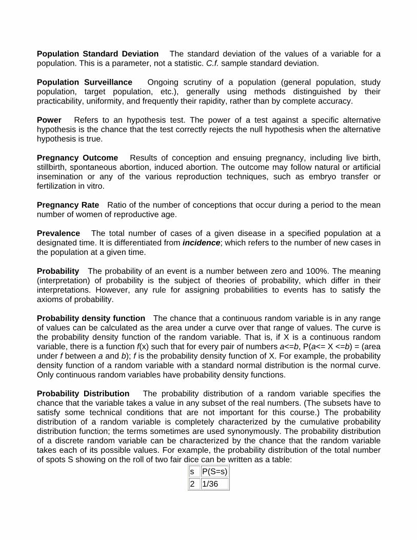
Population Standard Deviation The standard deviation of the values of a variable for a population. This is a parameter, not a statistic. C.f. sample standard deviation.

Population Surveillance Ongoing scrutiny of a population (general population, study population, target population, etc.), generally using methods distinguished by their practicability, uniformity, and frequently their rapidity, rather than by complete accuracy.

Power Refers to an hypothesis test. The power of a test against a specific alternative hypothesis is the chance that the test correctly rejects the null hypothesis when the alternative hypothesis is true.

Pregnancy Outcome Results of conception and ensuing pregnancy, including live birth, stillbirth, spontaneous abortion, induced abortion. The outcome may follow natural or artificial insemination or any of the various reproduction techniques, such as embryo transfer or fertilization in vitro.

Pregnancy Rate Ratio of the number of conceptions that occur during a period to the mean number of women of reproductive age.

Prevalence The total number of cases of a given disease in a specified population at a designated time. It is differentiated from incidence; which refers to the number of new cases in the population at a given time.

Probability The probability of an event is a number between zero and 100%. The meaning (interpretation) of probability is the subject of theories of probability, which differ in their interpretations. However, any rule for assigning probabilities to events has to satisfy the axioms of probability.

Probability density function The chance that a continuous random variable is in any range of values can be calculated as the area under a curve over that range of values. The curve is the probability density function of the random variable. That is, if X is a continuous random variable, there is a function f(x) such that for every pair of numbers a<=b, P(a<= X <=b) = (area under f between a and b); f is the probability density function of X. For example, the probability density function of a random variable with a standard normal distribution is the normal curve. Only continuous random variables have probability density functions. Probability Distribution The probability distribution of a random variable specifies the chance that the variable takes a value in any subset of the real numbers. (The subsets have to satisfy some technical conditions that are not important for this course.) The probability distribution of a random variable is completely characterized by the cumulative probability distribution function; the terms sometimes are used synonymously. The probability distribution of a discrete random variable can be characterized by the chance that the random variable takes each of its possible values. For example, the probability distribution of the total number of spots S showing on the roll of two fair dice can be written as a table:

s P(S=s)2 1/36

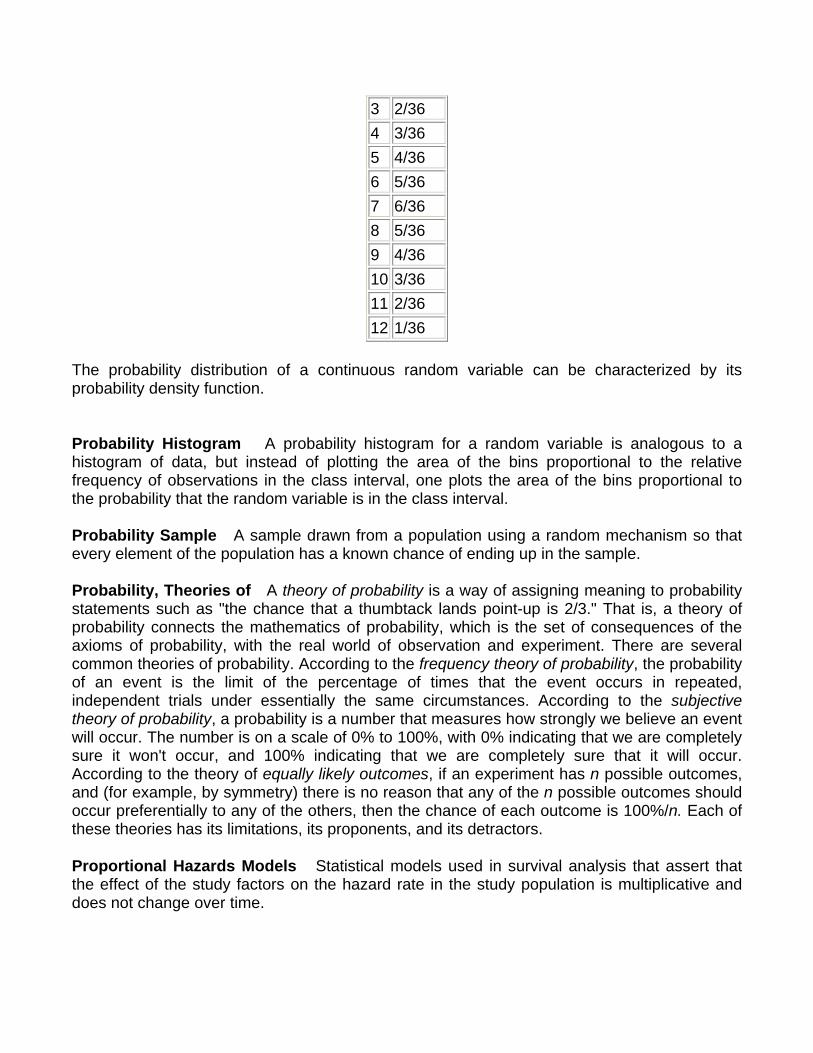
3 2/36 4 3/36 5 4/36 6 5/36 7 6/36 8 5/36 9 4/36 10 3/36 11 2/36 12 1/36

The probability distribution of a continuous random variable can be characterized by its probability density function.

Probability Histogram A probability histogram for a random variable is analogous to a histogram of data, but instead of plotting the area of the bins proportional to the relative frequency of observations in the class interval, one plots the area of the bins proportional to the probability that the random variable is in the class interval. Probability Sample A sample drawn from a population using a random mechanism so that every element of the population has a known chance of ending up in the sample. Probability, Theories of A theory of probability is a way of assigning meaning to probability statements such as "the chance that a thumbtack lands point-up is 2/3." That is, a theory of probability connects the mathematics of probability, which is the set of consequences of the axioms of probability, with the real world of observation and experiment. There are several common theories of probability. According to the frequency theory of probability, the probability of an event is the limit of the percentage of times that the event occurs in repeated, independent trials under essentially the same circumstances. According to the subjective theory of probability, a probability is a number that measures how strongly we believe an event will occur. The number is on a scale of 0% to 100%, with 0% indicating that we are completely sure it won't occur, and 100% indicating that we are completely sure that it will occur. According to the theory of equally likely outcomes, if an experiment has n possible outcomes, and (for example, by symmetry) there is no reason that any of the n possible outcomes should occur preferentially to any of the others, then the chance of each outcome is 100%/n. Each of these theories has its limitations, its proponents, and its detractors.

Proportional Hazards Models Statistical models used in survival analysis that assert that the effect of the study factors on the hazard rate in the study population is multiplicative and does not change over time.

Proposition, logical proposition A logical proposition is a statement that can be either true or false. For example, "the sun is shining in Berkeley right now" is a proposition.

top

Q Qualitative Variable A qualitative variable is one whose values are adjectives, such as colors, genders, nationalities, etc. C.f. quantitative variable and categorical variable. Quantile The qth quantile of a list (0 < q <= 1) is the smallest number such that the fraction q or more of the elements of the list are less than or equal to it. I.e., if the list contains n numbers, the qth quantile, is the smallest number Q such that at least n×q elements of the list are less than or equal to Q. Quantitative Variable A variable that takes numerical values for which arithmetic makes sense, for example, counts, temperatures, weights, amounts of money, etc. For some variables that take numerical values, arithmetic with those values does not make sense; such variables are not quantitative. For example, adding and subtracting social security numbers does not make sense. Quantitative variables typically have units of measurement, such as inches, people, or pounds. Quartiles There are three quartiles. The first or lower quartile (LQ) of a list is a number (not necessarily a number in the list) such that at least 1/4 of the numbers in the list are no larger than it, and at least 3/4 of the numbers in the list are no smaller than it. The second quartile is the median. The third or upper quartile (UQ) is a number such that at least 3/4 of the entries in the list are no larger than it, and at least 1/4 of the numbers in the list are no smaller than it. To find the quartiles, first sort the list into increasing order. Find the smallest integer that is at least as big as the number of entries in the list divided by four. Call that integer k. The kth element of the sorted list is the lower quartile. Find the smallest integer that is at least as big as the number of entries in the list divided by two. Call that integer l. The lth element of the sorted list is the median. Find the smallest integer that is at least as large as the number of entries in the list times 3/4. Call that integer m. The mth element of the sorted list is the upper quartile.

Questionnaires Predetermined sets of questions used to collect data - clinical data, social status, occupational group, etc. The term is often applied to a self-completed survey instrument.

top

R Random Allocation A process involving chance used in therapeutic trials or other research endeavor for allocating experimental subjects, human or animal, between treatment and control groups, or among treatment groups. It may also apply to experiments on inanimate objects.

Random Error All measurements are subject to error, which can often be broken down into two components: a bias or systematic error, which affects all measurements the same way; and a random error, which is in general different each time a measurement is made, and behaves like a number drawn with replacement from a box of numbered tickets whose average is zero. Random Event See random experiment. Random Experiment An experiment or trial whose outcome is not perfectly predictable, but for which the long-run relative frequency of outcomes of different types in repeated trials is predictable. Note that "random" is different from "haphazard," which does not necessarily imply long-term regularity. Random Sample A random sample is a sample whose members are chosen at random from a given population in such a way that the chance of obtaining any particular sample can be computed. The number of units in the sample is called the sample size, often denoted n. The number of units in the population often is denoted N. Random samples can be drawn with or without replacing objects between draws; that is, drawing all n objects in the sample at once (a random sample without replacement), or drawing the objects one at a time, replacing them in the population between draws (a random sample with replacement). In a random sample with replacement, any given member of the population can occur in the sample more than once. In a random sample without replacement, any given member of the population can be in the sample at most once. A random sample without replacement in which every subset of n of the N units in the population is equally likely is also called a simple random sample. The term random sample with replacement denotes a random sample drawn in such a way that every n-tuple of units in the population is equally likely. See also probability sample. Random Variable A random variable is an assignment of numbers to possible outcomes of a random experiment. For example, consider tossing three coins. The number of heads showing when the coins land is a random variable: it assigns the number 0 to the outcome {T, T, T}, the number 1 to the outcome {T, T, H}, the number 2 to the outcome {T, H, H}, and the number 3 to the outcome {H, H, H}. Randomized Controlled Experiment An experiment in which chance is deliberately introduced in assigning subjects to the treatment and control groups. For example, we could write an identifying number for each subject on a slip of paper, stir up the slips of paper, and draw slips without replacement until we have drawn half of them. The subjects identified on the

slips drawn could then be assigned to treatment, and the rest to control. Randomizing the assignment tends to decrease confounding of the treatment effect with other factors, by making the treatment and control groups roughly comparable in all respects but the treatment. Randomized Controlled Trials Clinical trials that involve at least one test treatment and one control treatment, concurrent enrollment and follow-up of the test- and control-treated groups, and in which the treatments to be administered are selected by a random process, such as the use of a random-numbers table. Treatment allocations using coin flips, odd-even numbers, patient social security numbers, days of the week, medical record numbers, or other such pseudo- or quasi-random processes, are not truly randomized and trials employing any of these techniques for patient assignment are designated simply controlled clinical trials. Range The range of a set of numbers is the largest value in the set minus the smallest value in the set. Note that as a statistical term, the range is a single number, not a range of numbers.

Records The commitment in writing, as authentic evidence, of something having legal importance. The concept includes certificates of birth, death, etc., as well as hospital, medical, and other institutional records.

Registries The systems and processes involved in the establishment, support, management, and operation of registers, e.g., disease registers.

Regression Analysis Procedures for finding the mathematical function which best describes the relationship between a dependent variable and one or more independent variables. In linear regression the relationship is constrained to be a straight line and least-squares analysis is used to determine the best fit. In logistic regression the dependent variable is qualitative rather than continuously variable and likelihood functions are used to find the best relationship. In multiple regression the dependent variable is considered to depend on more than a single independent variable. Regression, Linear Regression Linear regression fits a line to a scatterplot in such a way as to minimize the sum of the squares of the residuals. The resulting regression line, together with the standard deviations of the two variables or their correlation coefficient, can be a reasonable summary of a scatterplot if the scatterplot is roughly football-shaped. In other cases, it is a poor summary. If we are regressing the variable Y on the variable X, and if Y is plotted on the vertical axis and X is plotted on the horizontal axis, the regression line passes through the point of averages, and has slope equal to the correlation coefficient times the SD of Y divided by the SD of X. Regression Fallacy The regression fallacy is to attribute the regression effect to an external cause. Regression Toward the Mean, Regression Effect Suppose one measures two variables for each member of a group of individuals, and that the correlation coefficient of the variables is positive (negative). If the value of the first variable for that individual is above average, the

value of the second variable for that individual is likely to be above (below) average, but by fewer standard deviations than the first variable is. That is, the second observation is likely to be closer to the mean in standard units. For example, suppose one measures the heights of fathers and sons. Each individual is a (father, son) pair; the two variables measured are the height of the father and the height of the son. These two variables will tend to have a positive correlation coefficient: fathers who are taller than average tend to have sons who are taller than average. Consider a (father, son) pair chosen at random from this group. Suppose the father's height is 3SD above the average of all the fathers' heights. (The SD is the standard deviation of the fathers' heights.) Then the son's height is also likely to be above the average of the sons' heights, but by fewer than 3SD (here the SD is the standard deviation of the sons' heights).

Relative Risk Assessment An evaluation of the risk of disease in a patient who possesses a certain characteristic relative to one who does not possess that characteristic. Relative risk can be assessed as a property of a clinical test.

Relative Risk Reduction (RRR) The proportional reduction in outcome rates between control and experimental patients in a trial.

Repeated Measures Analysis of Variance An ANOVA that analyzes two or more related measurements of the same variable.

Reproducibility of Results The statistical reproducibility of measurements (often in a clinical context), including the testing of instrumentation or techniques to obtain reproducible results. The concept includes reproducibility of physiological measurements, which may be used to develop rules to assess probability or prognosis, or response to a stimulus; reproducibility of occurrence of a condition; and reproducibility of experimental results.

Reproductive History An important aggregate factor in epidemiological studies of women's health. The concept usually includes the number and timing of pregnancies and their outcomes, the incidence of breast feeding, and may include age of menarche and menopause, regularity of menstruation, fertility, gynecological or obstetric problems, or contraceptive usage.

Residence Characteristics Elements of residence that characterize a population. They are applicable in determining need for and utilization of health services

Residential Mobility Frequent change of residence, either in the same city or town, or between cities, states or communities.

Residual The difference between a datum and the value predicted for it by a model. In linear regression of a variable plotted on the vertical axis onto a variable plotted on the horizontal axis, a residual is the "vertical" distance from a datum to the line. Residuals can be positive (if the datum is above the line) or negative (if the datum is below the line). Plots of residuals can reveal computational errors in linear regression, as well as conditions under which linear regression is inappropriate, such as nonlinearity and heteroscedasticity. If linear regression is

performed properly, the sum of the residuals from the regression line must be zero; otherwise, there is a computational error somewhere. Residual Plot A residual plot for a regression is a plot of the residuals from the regression against the explanatory variable. Resistant A statistic is said to be resistant if corrupting a datum cannot change the statistic much. The mean is not resistant; the median is.

Risk The probability that an event will occur. It encompasses a variety of measures of the probability of a generally unfavorable outcome.

Risk Assessment The qualitative or quantitative estimation of the likelihood of adverse effects that may result from exposure to specified health hazards or from the absence of beneficial influences.

Risk Factors An aspect of personal behavior or lifestyle, environmental exposure, or inborn or inherited characteristic, which, on the basis of epidemiologic evidence, is known to be associated with a health-related condition considered important to prevent.

Root-mean-square (RMS) The RMS of a list is the square-root of the mean of the squares of the elements in the list. It is a measure of the average "size" of the elements of the list. To compute the RMS of a list, you square all the entries, average the numbers you get, and take the square-root of that average. Root-mean-square error (RMSE) The RMSE of an estimator of a parameter is the square-root of the mean squared error (MSE) of the estimator. In symbols, if X is an estimator of the parameter t, then RMSE(X) = ( E( (X-t)2 ) )½. The RMSE of an estimator is a measure of the expected error of the estimator. The units of RMSE are the same as the units of the estimator. See also mean squared error. rms Error of Regression The rms error of regression is the rms of the vertical residuals from the regression line. For regressing Y on X, the rms error of regression is equal to (1 - r2)½×SDY, where r is the correlation coefficient between X and Y and SDY is the standard deviation of the values of Y.

top

S

Sample A sample is a collection of units from a population. See also random sample.

Sample Mean The arithmetic mean of a random sample from a population. It is a statistic commonly used to estimate the population mean. Suppose there are n data, {x1, x2, . . . , xn}. The sample mean is (x1 + x2 + . . . + xn)/n. The expected value of the sample mean is the population mean. For sampling with replacement, the SE of the sample mean is the population standard deviation, divided by the square-root of the sample size. For sampling without replacement, the SE of the sample mean is the finite-population correction ((N-n)/(N-1))½ times the SE of the sample mean for sampling with replacement, with N the size of the population and n the size of the sample. Sample Percentage The percentage of a random sample with a certain property, such as the percentage of voters registered as Democrats in a simple random sample of voters. The sample mean is a statistic commonly used to estimate the population percentage. The expected value of the sample percentage from a simple random sample or a random sample with replacement is the population percentage. The SE of the sample percentage for sampling with replacement is (p(1-p)/n )½, where p is the population percentage and n is the sample size. The SE of the sample percentage for sampling without replacement is the finite-population correction ((N-n)/(N-1))½ times the SE of the sample percentage for sampling with replacement, with N the size of the population and n the size of the sample. The SE of the sample percentage is often estimated by the bootstrap.

Sample Size The number of units (persons, animals, patients, specified circumstances, etc.) in a population to be studied. The sample size should be big enough to have a high likelihood of detecting a true difference between two groups.

Sample Standard Deviation, S The sample standard deviation S is an estimator of the standard deviation of a population based on a random sample from the population. The sample standard deviation is a statistic that measures how "spread out" the sample is around the sample mean. It is quite similar to the standard deviation of the sample, but instead of averaging the squared deviations (to get the rms of the deviations of the data from the sample mean) it divides the sum of the squared deviations by (number of data - 1) before taking the square-root. Suppose there are n data, {x1, x2, . . . , xn}, with mean M = (x1 + x2 + . . . + xn)/n. Then s = ( ((x1 - M)2 + (x2 - M)2 + . . . + (xn - M)2)/(n-1) )½ . The square of the sample standard deviation, S2 (the sample variance) is an unbiased estimator of the square of the SD of the population (the variance of the population). Sample Sum The sum of a random sample from a population. The expected value of the sample sum is the sample size times the population mean. For sampling with replacement, the SE of the sample sum is the population standard deviation, times the square-root of the sample size. For sampling without replacement, the SE of the sample sum is the finite-population correction ((N-n)/(N-1))½ times the SE of the sample sum for sampling with replacement, with N the size of the population and n the size of the sample. Sample Survey A survey based on the responses of a sample of individuals, rather than the entire population.

Sample Variance The sample variance is the square of the sample standard deviation S. It is an unbiased estimator of the square of the population standard deviation, which is also called the variance of the population. Sampling distribution The sampling distribution of an estimator is the probability distribution of the estimator when it is applied to random samples. Sampling error In estimating from a random sample, the difference between the estimator and the parameter can be written as the sum of two components: bias and sampling error. The bias is the average error of the estimator over all possible samples. The bias is not random. Sampling error is the component of error that varies from sample to sample. The sampling error is random: it comes from "the luck of the draw" in which units happen to be in the sample. It is the chance variation of the estimator. The average of the sampling error over all possible samples (the expected value of the sampling error) is zero. The standard error of the estimator is a measure of the typical size of the sampling error.

Sampling Studies Studies in which a number of subjects are selected from all subjects in a defined population. Conclusions based on sample results may be attributed only to the population sampled.

Sampling unit A sample from a population can be drawn one unit at a time, or more than one unit at a time (one can sample clusters of units). The fundamental unit of the sample is called the sampling unit. It need not be a unit of the population. Scatterplot A scatterplot is a way to visualize bivariate data. A scatterplot is a plot of pairs of measurements on a collection of "individuals" (which need not be people). For example, suppose we record the heights and weights of a group of 100 people. The scatterplot of those data would be 100 points. Each point represents one person's height and weight. In a scatterplot of weight against height, the x-coordinate of each point would be height of one person, the y-coordinate of that point would be the weight of the same person. In a scatterplot of height against weight, the x-coordinates would be the weights and the y-coordinates would be the heights. SD line For a scatterplot, a line that goes through the point of averages, with slope equal to the ratio of the standard deviations of the two plotted variables. If the variable plotted on the horizontal axis is called X and the variable plotted on the vertical axis is called Y, the slope of the SD line is the SD of Y, divided by the SD of X. Secular Trend A linear association (trend) with time. Selection Bias A systematic tendency for a sampling procedure to include and/or exclude units of a certain type. For example, in a quota sample, unconscious prejudices or predilections on the part of the interviewer can result in selection bias. Selection bias is a potential problem whenever a human has latitude in selecting individual units for the sample; it tends to be eliminated by probability sampling schemes in which the interviewer is told exactly whom to contact (with no room for individual choice).

Self-Selection Self-selection occurs when individuals decide for themselves whether they are in the control group or the treatment group. Self-selection is quite common in studies of human behavior. For example, studies of the effect of smoking on human health involve self-selection: individuals choose for themselves whether or not to smoke. Self-selection precludes an experiment; it results in an observational study. When there is self-selection, one must be wary of possible confounding from factors that influence individuals' decisions to belong to the treatment group. Sensitivity Measures for assessing the results of diagnostic and screening tests. Sensitivity represents the proportion of truly diseased persons in a screened population who are identified as being diseased by the test. It is a measure of the probability of correctly diagnosing a condition.

Sentinel Surveillance Monitoring of rate of occurrence of specific conditions to assess the stability or change in health levels of a population. It is also the study of disease rates in a specific cohort, geographic area, population subgroup, etc. to estimate trends in larger population.

Set A set is a collection of things, without regard to their order. Significance, Significance level, Statistical significance The significance level of an hypothesis test is the chance that the test erroneously rejects the null hypothesis when the null hypothesis is true. Simple Random Sample A simple random sample of n units from a population is a random sample drawn by a procedure that is equally likely to give every collection of n units from the population; that is, the probability that the sample will consist of any given subset of n of the N units in the population is 1/NCn. Simple random sampling is sampling at random without replacement (without replacing the units between draws). A simple random sample of size n from a population of N >= n units can be constructed by assigning a random number between zero and one to each unit in the population, then taking those units that were assigned the n largest random numbers to be the sample. Simpson's Paradox What is true for the parts is not necessarily true for the whole. See also confounding. Single-Blind Method A method in which either the observer(s) or the subject(s) is kept ignorant of the group to which the subjects are assigned. Skewed Distribution A distribution that is not symmetrical.

Specificity Measures for assessing the results of diagnostic and screening tests. Specificity is the proportion of truly non-diseased persons who are so identified by the screening test. It is a measure of the probability of correctly identifying a non-diseased person.

Severity of Illness Index Levels of severity of illness within a diagnostic group which are established by various measurement criteria.

Sex Distribution The number of males and females in a given population. The distribution may refer to how many men or women or what proportion of either in the group. The population is usually patients with a specific disease but the concept is not restricted to humans and is not restricted to medicine.

Sickness Impact Profile A quality-of-life scale developed in the United States in 1972 as a measure of health status or dysfunction generated by a disease. It is a behaviorally based questionnaire for patients and addresses activities such as sleep and rest, mobility, recreation, home management, emotional behavior, social interaction, and the like. It measures the patient's perceived health status and is sensitive enough to detect changes or differences in health status occurring over time or between groups.

Small-Area Analysis A method of analyzing the variation in utilization of health care in small geographic or demographic areas. It often studies, for example, the usage rates for a given service or procedure in several small areas, documenting the variation among the areas. By comparing high- and low-use areas, the analysis attempts to determine whether there is a pattern to such use and to identify variables that are associated with and contribute to the variation.

Space-Time Clustering A statistically significant excess of cases of a disease, occurring within a limited space-time continuum.

Square-Root Law The Square-Root Law says that the standard error (SE) of the sample sum of n random draws with replacement from a box of tickets with numbers on them is... SE(sample sum) = n½×SD(box), and the standard error of the sample mean of n random draws with replacement from a box of tickets is... SE(sample mean) = n-½×SD(box), where SD(box) is the standard deviation of the list of the numbers on all the tickets in the box (including repeated values). Standard Deviation (SD) The standard deviation of a set of numbers is the rms of the set of deviations between each element of the set and the mean of the set. See also sample standard deviation. Standard Error (SE) The Standard Error of a random variable is a measure of how far it is likely to be from its expected value; that is, its scatter in repeated experiments. The SE of a random variable X is defined to be... SE(X) = [E( (X - E(X))2 )] ½. That is, the standard error is the square-root of the expected squared difference between the random variable and its expected value. The SE of a random variable is analogous to the SD of a list. Standard Units A variable (a set of data) is said to be in standard units if its mean is zero and its standard deviation is one. You transform a set of data into standard units by subtracting the mean from each element of the list, and dividing the results by the standard deviation. A random variable is said to be in standard units if its expected value is zero and its standard

error is one. You transform a random variable to standard units by subtracting its expected value then dividing by its standard error. Standardize To transform into standard units. Statistic A number that can be computed from data, involving no unknown parameters. As a function of a random sample, a statistic is a random variable. Statistics are used to estimate parameters, and to test hypotheses.

Statistical Distributions The complete summaries of the frequencies of the values or categories of a measurement made on a group of items, a population, or other collection of data. The distribution tells either how many or what proportion of the group was found to have each value (or each range of values) out of all the possible values that the quantitative measure can have.

Stratified Sample In a stratified sample, subsets of sampling units are selected separately from different strata, rather than from the frame as a whole. Stratified sampling The act of drawing a stratified sample. Stratum In random sampling, sometimes the sample is drawn separately from different disjoint subsets of the population. Each such subset is called a stratum. (The plural of stratum is strata.) Samples drawn in such a way are called stratified samples. Estimators based on stratified random samples can have smaller sampling errors than estimators computed from simple random samples of the same size, if the average variability of the variable of interest within strata is smaller than it is across the entire population; that is, if stratum membership is associated with the variable. For example, to determine average home prices in the U.S., it would be advantageous to stratify on geography, because average home prices vary enormously with location. We might divide the country into states, then divide each state into urban, suburban, and rural areas; then draw random samples separately from each such division. Studentized score The observed value of a statistic, minus the expected value of the statistic, divided by the estimated standard error of the statistic. Student's t curve Student's t curve is a family of curves indexed by a parameter called the degrees of freedom, which can take the values 1, 2, . . . Student's t curve is used to approximate some probability histograms. Consider a population of numbers that are nearly normally distributed and have population mean is µ. Consider drawing a random sample of size n with replacement from the population, and computing the sample mean M and the sample standard deviation S define the random variable...T = (M - µ)/(S/n½). If the sample size n is large, the probability histogram of T can be approximated accurately by the normal curve. However, for small and intermediate values of n, Student's t curve with n - 1 degrees of freedom gives a better approximation. That is..... P(a < T < b) is approximately the area under Student's T curve with n - 1 degrees of freedom, from a to b. Student's t curve can be used to

test hypotheses about the population mean and construct confidence intervals for the population mean, when the population distribution is known to be nearly normally distributed. Subject, Experimental Subject A member of the control group or the treatment group. Subset A subset of a given set is a collection of things that belong to the original set. Every element of the subset must belong to the original set, but not every element of the original set need be in a subset (otherwise, a subset would always be identical to the set it came from).

Survival Analysis A class of statistical procedures for estimating the survival function (function of time, starting with a population 100% well at a given time and providing the percentage of the population still well at later times). The survival analysis is then used for making inferences about the effects of treatments, prognostic factors, exposures, and other covariates on the function.

Survival Rate The proportion of survivors in a group, e.g., of patients, studied and followed over a period, or the proportion of persons in a specified group alive at the beginning of a time interval who survive to the end of the interval. It is often studied using life table methods.

Symmetric Distribution The probability distribution of a random variable X is symmetric if there is a number a such that the chance that X>=a+b is the same as the chance that X<=a-b for every value of b. A list of numbers has a symmetric distribution if there is a number a such that the fraction of numbers in the list that are greater than or equal to a+b is the same as the fraction of numbers in the list that are less than or equal to a-b, for every value of b. In either case, the histogram or the probability histogram will be symmetrical about a vertical line drawn at x=a. Systematic error An error that affects all the measurements similarly. For example, if a ruler is too short, everything measured with it will appear to be longer than it really is (ignoring random error). If your watch runs fast, every time interval you measure with it will appear to be longer than it really is (again, ignoring random error). Systematic errors do not tend to average out. Systematic random sample A systematic sample starting at a random point in the listing of units in the of frame, instead of starting at the first unit. Systematic random sampling is better than systematic sampling, but typically not as good as simple random sampling. Systematic sample A systematic sample from a frame of units is one drawn by listing the units and selecting every kth element of the list. For example, if there are N units in the frame, and we want a sample of size N/10, we would take every tenth unit: the first unit, the eleventh unit, the 21st unit, etc. Systematic samples are not random samples, but they often behave essentially as if they were random, if the order in which the units appears in the list is haphazard. Systematic samples are a special case of cluster samples.

top

T t-Test A hypothesis test based on approximating the probability histogram of the test statistic by Student's t curve. t tests usually are used to test hypotheses about the mean of a population when the sample size is intermediate and the distribution of the population is known to be nearly normal. Test Statistic A statistic used to test hypotheses. An hypothesis test can be constructed by deciding to reject the null hypothesis when the value of the test statistic is in some range or collection of ranges. To get a test with a specified significance level, the chance when the null hypothesis is true that the test statistic falls in the range where the hypothesis would be rejected must be at most the specified significance level. The Z statistic is a common test statistic. Transformation Transformations turn lists into other lists, or variables into other variables. For example, to transform a list of temperatures in degrees Celsius into the corresponding list of temperatures in degrees Fahrenheit, you multiply each element by 9/5, and add 32 to each product. This is an example of an affine transformation: multiply by something and add something (y = ax + b is the general affine transformation of x; it's the familiar equation of a straight line). In a linear transformation, you only multiply by something (y = ax). Affine transformations are used to put variables in standard units. In that case, you subtract the mean and divide the results by the SD. This is equivalent to multiplying by the reciprocal of the SD and adding the negative of the mean, divided by the SD, so it is an affine transformation. Affine transformations with positive multiplicative constants have a simple effect on the mean, median, mode, quartiles, and other percentiles: the new value of any of these is the old one, transformed using exactly the same formula. When the multiplicative constant is negative, the mean, median, mode, are still transformed by the same rule, but quartiles and percentiles are reversed: the qth quantile of the transformed distribution is the transformed value of the 1-qth quantile of the original distribution (ignoring the effect of data spacing). The effect of an affine transformation on the SD, range, and IQR, is to make the new value the old value times the absolute value of the number you multiplied the first list by: what you added does not affect them. Treatment The substance or procedure studied in an experiment or observational study. At issue is whether the treatment has an effect on the outcome or variable of interest. Treatment Effect The effect of the treatment on the variable of interest. Establishing whether the treatment has an effect is the point of an experiment. Treatment group The individuals who receive the treatment, as opposed to those in the control group, who do not.

Two-sided Hypothesis test C.f. one-sided test. An hypothesis test of the null hypothesis that the value of a parameter, µ, is equal to a null value, µ0, designed to have power against the alternative hypothesis that either µ < µ0 or µ > µ0 (the alternative hypothesis contains values on both sides of the null value). For example, a significance level 5%, two-sided z test of the null hypothesis that the mean of a population equals zero against the alternative that it is greater than zero would reject the null hypothesis for values of

|(sample mean)| |z| = ----------------- > 1.96. SE(sample mean)

Type I and Type II errors These refer to hypothesis testing. A Type I error occurs when the null hypothesis is rejected erroneously when it is in fact true. A Type II error occurs if the null hypothesis is not rejected when it is in fact false.

Trauma Severity Indices Systems for assessing, classifying, and coding injuries. These systems are used in medical records, surveillance systems, and state and national registries to aid in the collection and reporting of trauma.

Twin Studies Methods of detecting genetic etiology in human traits. The basic premise of twin studies is that monozygotic twins, being formed by the division of a single fertilized ovum, carry identical genes, while dizygotic twins, being formed by the fertilization of two ova by two different spermatozoa, are genetically no more similar than two siblings born after separate pregnancies.

top

U

Unbiased Not biased; having zero bias. Uncontrolled Experiment An experiment in which there is no control group; i.e., in which the method of comparison is not used: the experimenter decides who gets the treatment, but the outcome of the treated group is not compared with the outcome of a control group that does not receive treatment. Uncorrelated A set of bivariate data is uncorrelated if its correlation coefficient is zero. Two random variables are uncorrelated if the expected value of their product equals the product of their expected values. If two random variables are independent, they are uncorrelated. (The converse is not true in general.) Uncountable A set is uncountable if it is not countable.

Unimodal Having exactly one mode. Union The union of two or more sets is the set of objects contained by at least one of the sets. The union of the events A and B is denoted "A" plus "B", "A or B", and "AUB". C.f. intersection. Unit A member of a population. Univariate Having or having to do with a single variable. Some univariate techniques and statistics include the histogram, IQR, mean, median, percentiles, quantiles, and SD. C.f. bivariate. Upper Quartile (UQ) See quartiles.

top

V Variable A numerical value or a characteristic that can differ from individual to individual. Variance, population variance The variance of a list is the square of the standard deviation of the list, that is, the average of the squares of the deviations of the numbers in the list from their mean. The variance of a random variable X, Var(X), is the expected value of the squared difference between the variable and its expected value: Var(X) = E((X - E(X))2). The variance of a random variable is the square of the standard error (SE) of the variable. Venn Diagram A pictorial way of showing the relations among sets or events. The universal set or outcome space is usually drawn as a rectangle; sets are regions within the rectangle. The overlap of the regions corresponds to the intersection of the sets. If the regions do not overlap, the sets are disjoint. The part of the rectangle included in one or more of the regions corresponds to the union of the sets.

Vital Statistics Used for general articles concerning statistics of births, deaths, marriages, etc.

top

X

XOR, exclusive disjunction XOR is an operation on two logical propositions. If p and q are two propositions, (p XOR q) is a proposition that is true if either p is true or if q is true, but not both. (p XOR q) is logically equivalent to ((p OR q) AND NOT (p AND q)).

top

Z

z-score The observed value of the Z statistic. Z statistic A Z statistic is a test statistic whose distribution under the null hypothesis has expected value zero and can be approximated well by the normal curve. Usually, Z statistics are constructed by standardizing some other statistic. The Z statistic is related to the original statistic by... Z = (original - expected value of original)/SE(original). z-test An hypothesis test based on approximating the probability histogram of the Z statistic under the null hypothesis by the normal curve.