Embed Size (px)
Citation preview
Submitted to the Annals of Statistics
LOWER BOUNDS ON THE CONVERGENCE RATES OF
ADAPTIVE MCMC METHODS
By Scott C. Schmidler
and Dawn B. Woodard
Duke University and Cornell University
We consider the convergence properties of recently proposed adap-tive Markov chain Monte Carlo (MCMC) algorithms for approxima-tion of high-dimensional integrals arising in Bayesian analysis andstatistical mechanics. Despite their name, in the general case thesealgorithms produce non-Markovian, time-inhomogeneous, irreversiblestochastic processes. Nevertheless, we show that lower bounds onthe mixing times of these processes can be obtained using familiarideas of hitting times and conductance from the theory of reversibleMarkov chains. While loose in some cases, the bounds obtained aresufficient to demonstrate slow mixing of several recently proposedalgorithms including the adaptive Metropolis algorithm of Haarioet al. (2001), the equi-energy sampler (Kou et al., 2006), and theimportance-resampling MCMC algorithm (Atchade, 2009b) on somemultimodal target distributions including mixtures of normal distri-butions and the mean-field Potts model. These results appear to bethe first non-trivial bounds on the mixing times of adaptive MCMCsamplers, and suggest that the adaptive methods considered may notprovide qualitative improvements in mixing over the simpler Markovchain algorithms on which they are based. Our bounds also indicateproperties which adaptive MCMC algorithms must have to achieveexponential speed-ups, suggesting directions for further research inthese methods.
1. Introduction. Markov chain Monte Carlo (MCMC) sampling tech-niques are currently the most widely used approach to approximating thehigh-dimensional integrals arising in Bayesian statistics, as well as in relatedareas such as statistical mechanics. As such, derivation of new MCMC meth-ods, and formal analysis of their properties, has become an important area ofBayesian statistics research (Andrieu and Roberts, 2009; Douc et al., 2007;Ji and Schmidler, 2009; Jones and Hobert, 2001; Kou et al., 2006; Mengersenand Tweedie, 1996; Mira, 2001; Neal, 2003; Roberts and Rosenthal, 2001;Tierney, 1994).
A common construction for MCMC utilizes a (Metropolis-Hastings) ran-dom walk that explores the state space via local moves; however, for some
Keywords and phrases: adaptive Monte Carlo, Markov chain convergence, equi-energysampler, rapid mixing, tempering
1imsart-aos ver. 2009/05/21 file: AdaptiveLowerBounds.tex date: July 16, 2010
2 SCHMIDLER & WOODARD
target distributions this random walk takes an impractically long time toexplore the target distribution. For example, when the target distributionis multimodal, a local random walk may rarely move between modes. Manyalgorithms have been introduced to address the challenge of efficient sam-pling from high-dimensional and multimodal distributions. Parallel temper-ing (Geyer, 1991) supplements a basic Metropolis-Hastings chain with a setof auxiliary chains, the states of which are occasionally swapped, “seeding”the primary chain with samples from other chains. These auxiliary chainsare typically constructed via a temperature parameter, which flattens thetarget distribution in order to enable crossing of energy barriers (regionsof low density), and can allow rapid movement between multiple modes.The related technique of simulated tempering (Geyer and Thompson, 1995;Marinari and Parisi, 1992) uses a single chain with alternating transitionkernels.
An alternative is to adapt the transition kernel of the chain, using informa-tion obtained from previous iterations to speed convergence - such methodsare termed adaptive MCMC. The recently proposed equi-energy sampler(Kou et al., 2006), like parallel tempering, constructs auxiliary samplingchains typically constructed by temperature. However, rather than swap-ping, the equi-energy sampler seeds the primary chain with proposed jumpsto locations visited previously by the other chains, specifically those lo-cations having approximately equal energy (density) to the current state.Such jumps potentially enable movement between distinct modes of the tar-get distribution. Two other adaptive algorithms, the importance-resamplingMCMC (IR-MCMC) algorithm (Atchade, 2009b) and a method proposed byGelfand and Sahu (1994), also utilize multiple (non-Markovian) processeswhich can supplement local moves with jumps to locations previously vis-ited by another process. Again, these methods aim to improve upon theefficiency of a single Markov chain.
Such adaptive algorithms have been shown empirically to have morerapid convergence and more rapid decay of autocorrelation than their non-adaptive counterparts on several examples (Kou et al., 2006; Minary andLevitt, 2006). However, Atchade (2009a) gives an example for which theempirical performance of the equi-energy sampler and IR-MCMC is compa-rable to that of random-walk Metropolis, and argues that the equi-energyand IR-MCMC samplers are not themselves asymptotically as efficient astheir (very efficient) limiting kernels.
Few rigorous bounds on the convergence rates of adaptive MCMC tech-niques are available. Andrieu and Moulines (2006) and Andrieu and Atchade(2007) obtain asymptotic efficiency results for a different class of adaptive
imsart-aos ver. 2009/05/21 file: AdaptiveLowerBounds.tex date: July 16, 2010
CONVERGENCE OF ADAPTIVE MCMC 3
MCMC techniques which tune parameters of a parametric transition kernel.Atchade (2009b) considers an adaptive process that at some fixed set of timesjumps back to a previously visited location, and shows that if the underlyingprocess converges geometrically then the adaptive process converges at leastpolynomially (in the number of steps n, not in problem size).
Here we consider the non-asymptotic behavior of such adaptive algo-rithms, specifically whether they yield convergence (“mixing”) times thatimprove significantly on their non-adaptive counterparts. A major obstacleto obtaining non-asymptotic bounds is the non-Markovian, time-inhomogeneous, irreversible nature of the algorithms, preventing direct ap-plication of spectral analysis and other common methods used for Markovchains. Our main result (Theorem 4.1) extends a bound by Woodard et al.(2009b) for parallel and simulated tempering to these adaptive methods.For a single process, the bound shows that the mixing time of the adaptivesampler, like that of the underlying Markov chain on which it is based, islimited by the conductance of the Markov kernel (Corollary 4.1). This resultholds irrespective of how the non-local jumps are taken and the values ofany adaptation tuning parameters. Therefore this type of adaptivity, whichwe call multichain resampling, cannot provide a qualitative speedup fromslow to rapid mixing (defined formally in Section 3). This result is not im-mediately obvious since it might seem advantageous, if the current routeof exploration proves unfruitful, to jump back to a more promising loca-tion and restart exploration from that point. The same result holds for themulti-process sampler of Gelfand and Sahu (1994), regardless of the numberof processes. Combined with results obtained by Woodard et al. (2009b), ourbounds immediately imply that multichain resampling methods (includingthe equi-energy sampler, IR-MCMC, and Gelfand-Sahu sampler) mix slowlyon two examples considered there: mixtures of normal distributions in R
d,and the mean-field ferromagnetic Potts model.
Our results formalize the intuitive notion that jumping back to locationsalready visited cannot speed exploration of new, as yet unseen, regions ofthe target distribution. However, such adaptation may indeed yield improve-ments in autocorrelation times (and hence asymptotic efficiency) relative totheir non-adaptive counterparts. Indeed, this is suggested by the empiricalresults demonstrated in these papers. However, our lower bounds indicatethat qualitative improvements in convergence to equilibrium may not beobtainable under the type of adaptivity utilized in these algorithms. In-stead, algorithms that encourage exploration of new regions, in additionto speeding mixing among previously visited regions, must be explored. Apreliminary step in this direction is given by Heaton and Schmidler (2009).
imsart-aos ver. 2009/05/21 file: AdaptiveLowerBounds.tex date: July 16, 2010
4 SCHMIDLER & WOODARD
In Section 2 we define the class of adaptive methods under consideration.Section 3 obtains bounds on the mixing time of these techniques and relatesthem to existing results on Markov chains. Section 5 shows slow mixing onthe two examples, and we conclude with some discussion in Section 7.
2. Adaptive MCMC Techniques. We divide adaptive MCMC tech-niques considered here into two classes, which capture the majority of meth-ods proposed to date. The first class simulates one or more parallel chains,and for each chain i attempts to adaptively optimize over a family of tran-sition kernels {Tθ : θ ∈ Θ(i)} that are invariant with respect to the targetdistribution of that chain. We call these methods invariant adaptive Markovchain (IAMC) methods. The second class also simulates one or more paral-lel chains, but sometimes resamples from the history of the chains in orderto share information among the chains, or to speed mixing among previ-ously visited regions. The transition kernels of such methods generally areonly invariant with respect to the target distribution in a limiting sense. Wecall these methods multichain resampling adaptive Markov chain (MRAM)methods.
To fix notation, let π denote the target distribution of interest on statespace X . Let X(1), . . . ,X(I) be a set of discrete time stochastic processes
X(i) = X(i)0 ,X
(i)1 , . . . on X , targeted at distributions π(i). At least one X(i)
is assumed to have π(i) = π; call it X(1).
2.1. IAMC Methods. The most familiar approach to adapting MCMCsamplers is to optimize the proposal kernel of a Metropolis-Hastings chain.More generally, let {Tθ}θ∈Θ(i) be a set of ergodic, π(i)-reversible Markov
transition kernels on X , and denote by X(i)0:n−1 the history of the ith process
at time n. We consider adaptive sampling algorithms for which the X(i) aregenerated by respective time-inhomogeneous but π(i)-invariant transition
kernels Ti,n = Tθi,nwhere θi,n = gi(X
(1:I)0:n−1) ∈ Θ(i). We call such algorithms
IAMC methods. Here gi are functions defining the adaptation; IAMC meth-ods are typically constructed to ensure θi,n
n→∞−→ θ∗ for some optimal valueθ∗, but our results do not depend on this property. For concreteness we re-strict to the case π(i) ≡ π and Θ(i) ≡ Θ for a common set Θ, which capturesall such algorithms proposed to date.
Adaptive Metropolis. The adaptive Metropolis scheme of Haario et al. (2001)was the first of this type to provide formal proof of convergence under con-tinuous adaptation, and helped spark a resurgence of interest in adaptiveMCMC methods. The Haario et al. (2001) scheme uses a single chain withπ-invariant Metropolis-Hastings kernels Tθ on X = R
d constructed from a
imsart-aos ver. 2009/05/21 file: AdaptiveLowerBounds.tex date: July 16, 2010
CONVERGENCE OF ADAPTIVE MCMC 5
multivariate normal random-walk proposal. The adaptive parameter θ is thecovariance matrix of the random-walk proposal.
Parallel Chains. Craiu et al. (2009) propose simulating parallel Metropolis-Hastings chains with common invariant distribution π and a common pro-posal kernel Pθ, adapting the parameters of that kernel using the past sam-ples from all of the chains (“Inter-chain Adaptation”).
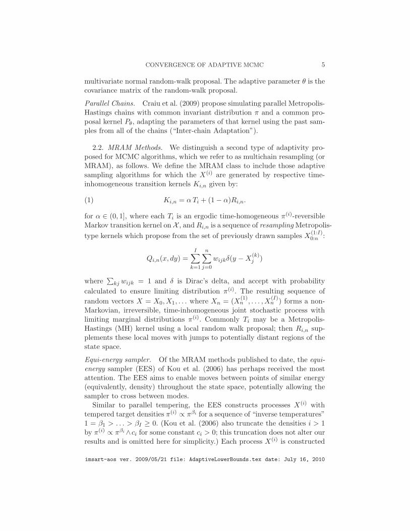
2.2. MRAM Methods. We distinguish a second type of adaptivity pro-posed for MCMC algorithms, which we refer to as multichain resampling (orMRAM), as follows. We define the MRAM class to include those adaptivesampling algorithms for which the X(i) are generated by respective time-inhomogeneous transition kernels Ki,n given by:
(1) Ki,n = αTi + (1 − α)Ri,n.
for α ∈ (0, 1], where each Ti is an ergodic time-homogeneous π(i)-reversibleMarkov transition kernel on X , andRi,n is a sequence of resampling Metropolis-
type kernels which propose from the set of previously drawn samples X(1:I)0:n :
Qi,n(x, dy) =I∑
k=1
n∑
j=0
wijkδ(y −X(k)j )
where∑
kj wijk = 1 and δ is Dirac’s delta, and accept with probability
calculated to ensure limiting distribution π(i). The resulting sequence of
random vectors X = X0,X1, . . . where Xn = (X(1)n , . . . ,X
(I)n ) forms a non-
Markovian, irreversible, time-inhomogeneous joint stochastic process withlimiting marginal distributions π(i). Commonly Ti may be a Metropolis-Hastings (MH) kernel using a local random walk proposal; then Ri,n sup-plements these local moves with jumps to potentially distant regions of thestate space.
Equi-energy sampler. Of the MRAM methods published to date, the equi-energy sampler (EES) of Kou et al. (2006) has perhaps received the mostattention. The EES aims to enable moves between points of similar energy(equivalently, density) throughout the state space, potentially allowing thesampler to cross between modes.
Similar to parallel tempering, the EES constructs processes X(i) withtempered target densities π(i) ∝ πβi for a sequence of “inverse temperatures”1 = β1 > . . . > βI ≥ 0. (Kou et al. (2006) also truncate the densities i > 1by π(i) ∝ πβi ∧ci for some constant ci > 0; this truncation does not alter ourresults and is omitted here for simplicity.) Each process X(i) is constructed
imsart-aos ver. 2009/05/21 file: AdaptiveLowerBounds.tex date: July 16, 2010
6 SCHMIDLER & WOODARD
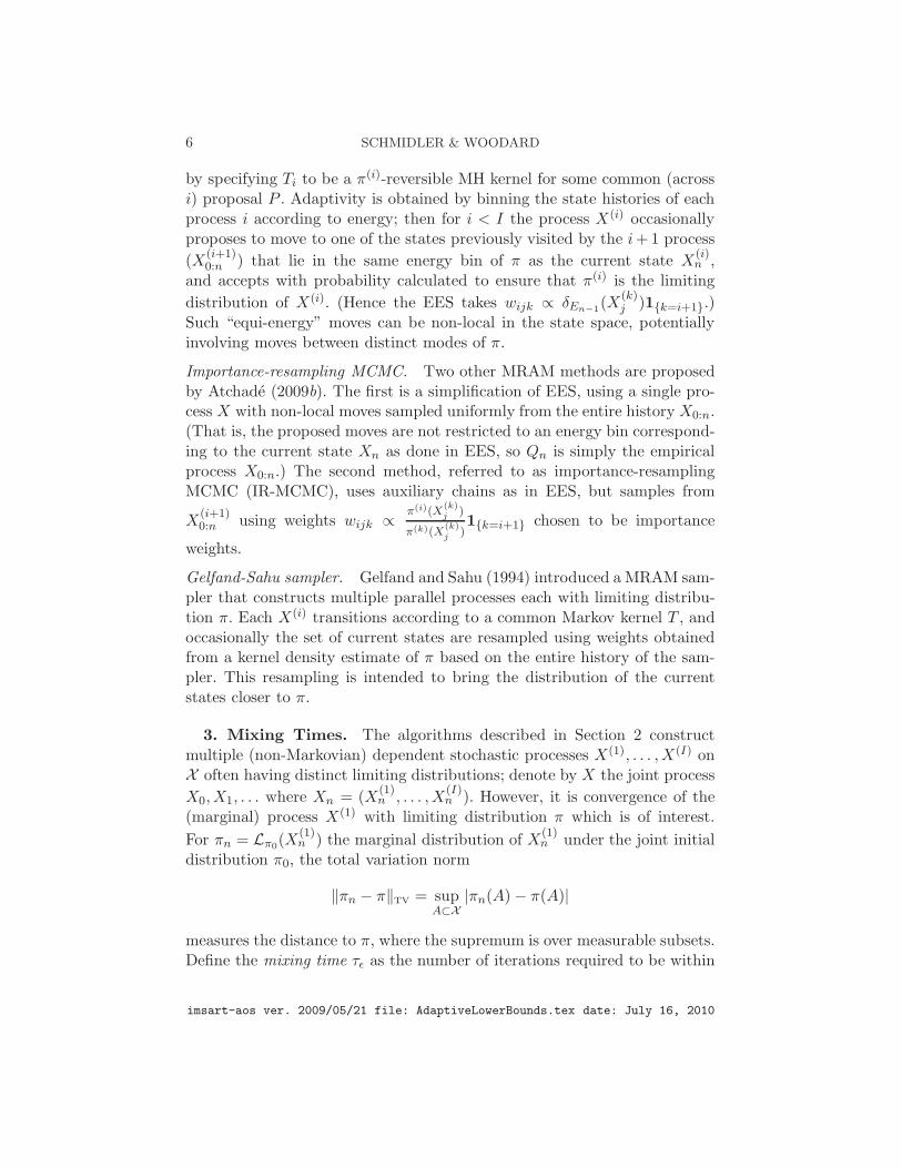
by specifying Ti to be a π(i)-reversible MH kernel for some common (acrossi) proposal P . Adaptivity is obtained by binning the state histories of eachprocess i according to energy; then for i < I the process X(i) occasionallyproposes to move to one of the states previously visited by the i+ 1 process
(X(i+1)0:n ) that lie in the same energy bin of π as the current state X
(i)n ,
and accepts with probability calculated to ensure that π(i) is the limiting
distribution of X(i). (Hence the EES takes wijk ∝ δEn−1(X(k)j )1{k=i+1}.)
Such “equi-energy” moves can be non-local in the state space, potentiallyinvolving moves between distinct modes of π.
Importance-resampling MCMC. Two other MRAM methods are proposedby Atchade (2009b). The first is a simplification of EES, using a single pro-cess X with non-local moves sampled uniformly from the entire history X0:n.(That is, the proposed moves are not restricted to an energy bin correspond-ing to the current state Xn as done in EES, so Qn is simply the empiricalprocess X0:n.) The second method, referred to as importance-resamplingMCMC (IR-MCMC), uses auxiliary chains as in EES, but samples from
X(i+1)0:n using weights wijk ∝ π(i)(X
(k)j
)
π(k)(X(k)j
)1{k=i+1} chosen to be importance
weights.
Gelfand-Sahu sampler. Gelfand and Sahu (1994) introduced a MRAM sam-pler that constructs multiple parallel processes each with limiting distribu-tion π. Each X(i) transitions according to a common Markov kernel T , andoccasionally the set of current states are resampled using weights obtainedfrom a kernel density estimate of π based on the entire history of the sam-pler. This resampling is intended to bring the distribution of the currentstates closer to π.
3. Mixing Times. The algorithms described in Section 2 constructmultiple (non-Markovian) dependent stochastic processes X(1), . . . ,X(I) onX often having distinct limiting distributions; denote by X the joint process
X0,X1, . . . where Xn = (X(1)n , . . . ,X
(I)n ). However, it is convergence of the
(marginal) process X(1) with limiting distribution π which is of interest.
For πn = Lπ0(X(1)n ) the marginal distribution of X
(1)n under the joint initial
distribution π0, the total variation norm
‖πn − π‖TV = supA⊂X
|πn(A) − π(A)|
measures the distance to π, where the supremum is over measurable subsets.Define the mixing time τǫ as the number of iterations required to be within
imsart-aos ver. 2009/05/21 file: AdaptiveLowerBounds.tex date: July 16, 2010
CONVERGENCE OF ADAPTIVE MCMC 7
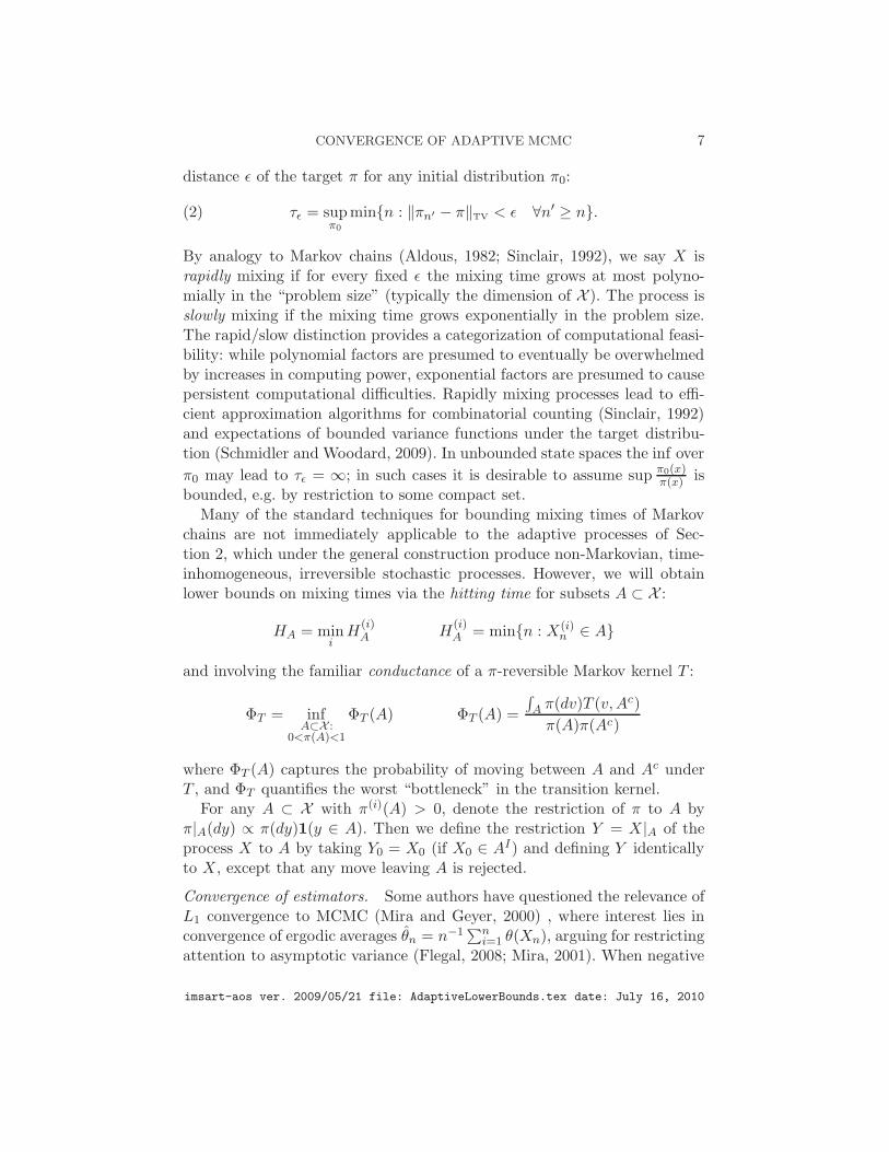
distance ǫ of the target π for any initial distribution π0:
(2) τǫ = supπ0
min{n : ‖πn′ − π‖TV < ǫ ∀n′ ≥ n}.
By analogy to Markov chains (Aldous, 1982; Sinclair, 1992), we say X israpidly mixing if for every fixed ǫ the mixing time grows at most polyno-mially in the “problem size” (typically the dimension of X ). The process isslowly mixing if the mixing time grows exponentially in the problem size.The rapid/slow distinction provides a categorization of computational feasi-bility: while polynomial factors are presumed to eventually be overwhelmedby increases in computing power, exponential factors are presumed to causepersistent computational difficulties. Rapidly mixing processes lead to effi-cient approximation algorithms for combinatorial counting (Sinclair, 1992)and expectations of bounded variance functions under the target distribu-tion (Schmidler and Woodard, 2009). In unbounded state spaces the inf over
π0 may lead to τǫ = ∞; in such cases it is desirable to assume sup π0(x)π(x) is
bounded, e.g. by restriction to some compact set.Many of the standard techniques for bounding mixing times of Markov
chains are not immediately applicable to the adaptive processes of Sec-tion 2, which under the general construction produce non-Markovian, time-inhomogeneous, irreversible stochastic processes. However, we will obtainlower bounds on mixing times via the hitting time for subsets A ⊂ X :
HA = miniH
(i)A H
(i)A = min{n : X(i)
n ∈ A}
and involving the familiar conductance of a π-reversible Markov kernel T :
ΦT = infA⊂X :
0<π(A)<1
ΦT (A) ΦT (A) =
∫
A π(dv)T (v,Ac)
π(A)π(Ac)
where ΦT (A) captures the probability of moving between A and Ac underT , and ΦT quantifies the worst “bottleneck” in the transition kernel.
For any A ⊂ X with π(i)(A) > 0, denote the restriction of π to A byπ|A(dy) ∝ π(dy)1(y ∈ A). Then we define the restriction Y = X|A of theprocess X to A by taking Y0 = X0 (if X0 ∈ AI) and defining Y identicallyto X, except that any move leaving A is rejected.
Convergence of estimators. Some authors have questioned the relevance ofL1 convergence to MCMC (Mira and Geyer, 2000) , where interest lies inconvergence of ergodic averages θn = n−1∑n
i=1 θ(Xn), arguing for restrictingattention to asymptotic variance (Flegal, 2008; Mira, 2001). When negative
imsart-aos ver. 2009/05/21 file: AdaptiveLowerBounds.tex date: July 16, 2010
8 SCHMIDLER & WOODARD
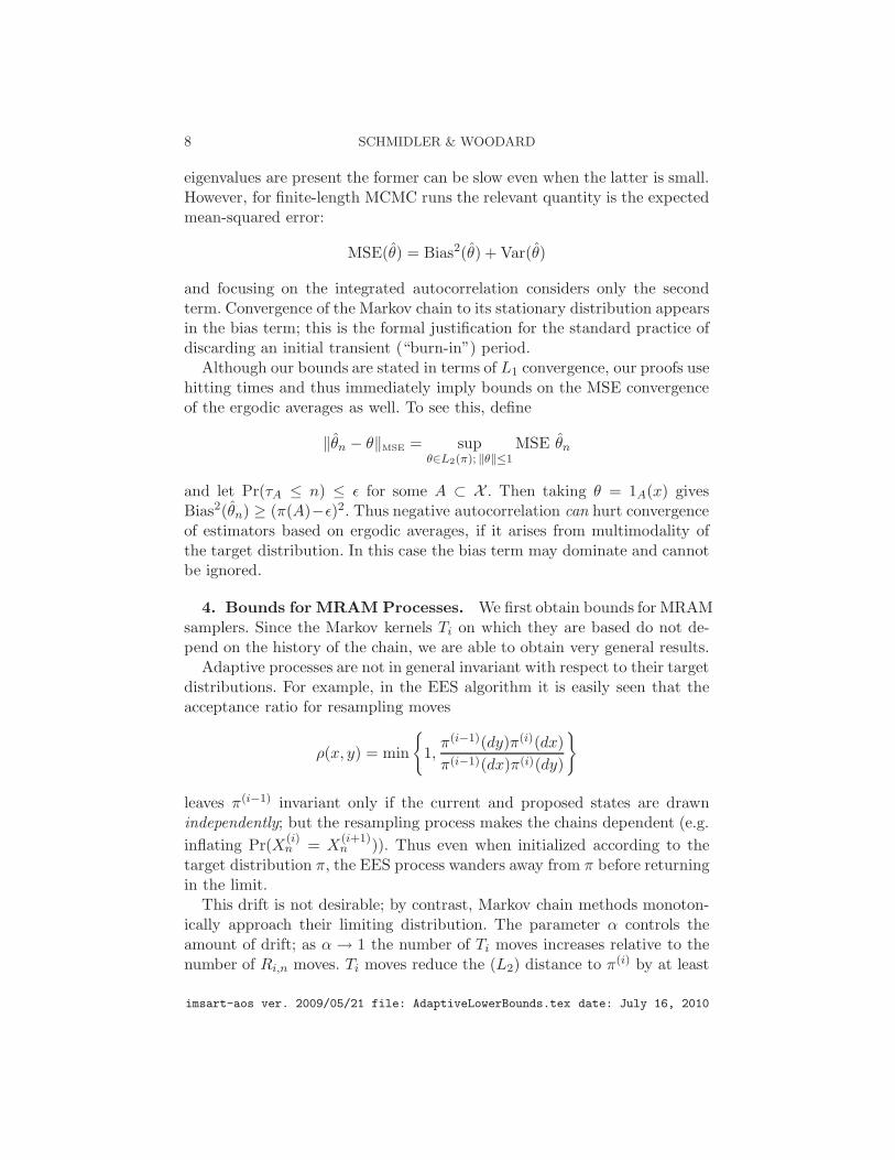
eigenvalues are present the former can be slow even when the latter is small.However, for finite-length MCMC runs the relevant quantity is the expectedmean-squared error:
MSE(θ) = Bias2(θ) + Var(θ)
and focusing on the integrated autocorrelation considers only the secondterm. Convergence of the Markov chain to its stationary distribution appearsin the bias term; this is the formal justification for the standard practice ofdiscarding an initial transient (“burn-in”) period.
Although our bounds are stated in terms of L1 convergence, our proofs usehitting times and thus immediately imply bounds on the MSE convergenceof the ergodic averages as well. To see this, define
‖θn − θ‖MSE = supθ∈L2(π); ‖θ‖≤1
MSE θn
and let Pr(τA ≤ n) ≤ ǫ for some A ⊂ X . Then taking θ = 1A(x) givesBias2(θn) ≥ (π(A)−ǫ)2. Thus negative autocorrelation can hurt convergenceof estimators based on ergodic averages, if it arises from multimodality ofthe target distribution. In this case the bias term may dominate and cannotbe ignored.
4. Bounds for MRAM Processes. We first obtain bounds for MRAMsamplers. Since the Markov kernels Ti on which they are based do not de-pend on the history of the chain, we are able to obtain very general results.
Adaptive processes are not in general invariant with respect to their targetdistributions. For example, in the EES algorithm it is easily seen that theacceptance ratio for resampling moves
ρ(x, y) = min
{
1,π(i−1)(dy)π(i)(dx)
π(i−1)(dx)π(i)(dy)
}
leaves π(i−1) invariant only if the current and proposed states are drawnindependently; but the resampling process makes the chains dependent (e.g.
inflating Pr(X(i)n = X
(i+1)n )). Thus even when initialized according to the
target distribution π, the EES process wanders away from π before returningin the limit.
This drift is not desirable; by contrast, Markov chain methods monoton-ically approach their limiting distribution. The parameter α controls theamount of drift; as α → 1 the number of Ti moves increases relative to thenumber of Ri,n moves. Ti moves reduce the (L2) distance to π(i) by at least
imsart-aos ver. 2009/05/21 file: AdaptiveLowerBounds.tex date: July 16, 2010
CONVERGENCE OF ADAPTIVE MCMC 9
a factor equal to the spectral gap of Ti, while Ri,n moves can inflate thisdistance. For α relatively large the drift should be minimal; in order to an-alyze adaptive methods in the presence of this drift, we assume that it isbounded as follows.
Assumption 4.1. There exists a constant 1 ≤ c < ∞ (independent ofproblem size) such that for any A ⊂ X having π(i)(A) > 0 for all i, the
sampler Y = X|A with Y(i)0
ind.∼ π(i)|A satisfies the following for all i and n:
the marginal distribution L(Y(i)n ) has a density with respect to π(i)|A that is
everywhere ≤ c.
This holds with c = 1 for the single-chain method of Atchade (2009b), andfor the degenerate case α = 1.
The bound we obtain for MRAM algorithms is a generalization of a mixingtime bound for parallel tempering given by Woodard et al. (2009b). Definethe persistence for any A ⊂ X and any i ∈ {1, . . . , I} as:
γ(A, i) = min
{
1,π(i)(A)
π(A)
}
.
Then the following bound for parallel tempering follows directly from thespectral gap bounds obtained in Woodard et al. (2009b):
Theorem A. (Woodard et al., 2009b)For X finite, ǫ > 0, and any A ⊂ X with 0 < π(i)(A) < 1 for all i, the
mixing time τ∗ǫ of parallel tempering satisfies
τ∗ǫ ≥ 2−8 ln(2ǫ)−1[
maxiγ(A, i)ΦTi
(A)
]−1/2
.
Now let X be a MRAM process on general X as defined in Section 2, satis-fying Assumption 4.1. We have the following result:
Theorem 4.1. For any ǫ > 0 and any A ⊂ X such that 0 < π(i)(A) < 1for all i, the mixing time τǫ of the MRAM process satisfies:
τǫ ≥ (π(A) − ǫ)
[
cImaxiγ(A, i)ΦTi
(A)
]−1
.
Proof. Let X(i)0
ind.∼ π(i)|Ac and let Y = X|Ac , so that ψi,n = L(Y(i)n ) has
a density with respect to π(i)|Ac that is everywhere ≤ c. Define the sequences
imsart-aos ver. 2009/05/21 file: AdaptiveLowerBounds.tex date: July 16, 2010
10 SCHMIDLER & WOODARD
Z(i) of Boolean random variables, where Z(i)n is true if a move of Y (i) at time
n is rejected because it would leave Ac, and false otherwise.
Consider the hitting time HA for X. Since H(1)A ≥ HA, for any n such
that Pr(HA ≤ n) ≤ π(A) − ǫ we have ‖πn − π‖TV ≥ ǫ and so τǫ > n. Theprobability that HA = n is equal to the probability that Y first attempts amove to A at time n but rejects due to restriction, so
Pr(HA ≤ n) ≤I∑
i=1
n∑
j=1
Pr(Z(i)j ) ≤
I∑
i=1
n∑
j=1
∫
AcTi(y,A)ψi,j−1(dy)
≤ cI∑
i=1
n∑
j=1
∫
AcTi(y,A)π(i)|Ac(dy)
= cnI∑
i=1
π(i)(A)ΦTi(A)
where the second inequality comes from the mixture representation of (1),since for the sampler Y we have Qi,j(y,A) = 0 for all y, i, and j. The lastequality uses reversibility of Ti. Now define nǫ(A) = min{n : Pr(HA ≤ n) >π(A) − ǫ}, so that
τǫ ≥ nǫ(A) ≥ (π(A) − ǫ)
[
c∑
i
π(i)(A)ΦTi(A)
]−1
≥ (π(A) − ǫ)
[
cI maxiπ(i)(A)ΦTi
(A)
]−1
.
Then π(i)(A) ≤ γ(A, i) gives the desired result.
The factor of I appearing in Theorem 4.1 but not Theorem A comesfrom the slightly different definitions of mixing in the two cases: the paralleltempering mixing time is for convergence of the joint chain process to itslimiting product distribution, required for the spectral analysis of Woodardet al. (2009b).
The difference in the dependence on ǫ between the two theorems comesfrom our use of hitting times to bound variation distance directly for thetime-inhomogeneous MRAM processes, compared to standard time-changearguments for time-homogeneous processes. We suspect this can be im-proved; the bound in Theorem 4.1 is certainly loose as a function of ǫ forsome MRAM processes, since parallel tempering is trivially in this set. How-ever, we can use Theorem 4.1 to analyze the effect of problem size on mixingtime for fixed ǫ (as in Section 5).
imsart-aos ver. 2009/05/21 file: AdaptiveLowerBounds.tex date: July 16, 2010
CONVERGENCE OF ADAPTIVE MCMC 11
4.1. Single Chain Resampling. Consider a MRAM process with a singlechain (I = 1), i.e. an adaptive process constructed from a Markov kernelT mixed with occasional jumps back to previously visited locations. Thesejumps can be made in any manner, subject to Assumption 4.1. In this case,Theorem 4.1 simplifies:
Corollary 4.1. For any 0 < ǫ < 1/4, the mixing time τǫ of a MRAMsampler based on T , with I = 1, satisfies:
τǫ ≥1
4cΦT.
Proof. For measurable A ⊂ X such that 1/2 ≤ π(A) < 1, Theorem 4.1gives τǫ ≥ (π(A) − ǫ)[cΦT (A)]−1, and the result follows from ǫ < 1/4 andΦT (A) = ΦT (Ac).
We can compare this result with standard results for Markov chains. Forthe case of X finite, if we assume that T (x, x) ≥ 3/4 for all x ∈ X (which canbe achieved by simply adding a holding probability of 3/4), results in Sinclair(1992) give the following bounds on the mixing time τ∗ǫ of the Markov chainT
(3)1
8ΦTln(2ǫ)−1 ≤ τ∗ǫ ≤ 8
Φ2T
[
ln(maxx
π(x)−1) + ln(ǫ−1)]
.
The lower bounds in (3) and Corollary 4.1 on the mixing times τ∗ǫ of theMarkov chain and τǫ of the adaptive sampler are of the same order as afunction of ΦT . Combining with results in Lawler and Sokal (1988) we have:
Corollary 4.2. For general X and T geometrically ergodic, if the spec-tral gap of T decreases exponentially in the problem size then any MRAMprocess based on T with I = 1 is slowly mixing.
Corollary 4.3. For finite X , if ln(maxx π(x)−1) grows polynomiallyas a function of the problem size, then slow mixing of the Markov chain withtransition kernel T implies slow mixing of any MRAM process based on Tthat has I = 1.
In particular, Corollary 4.2 proves for the first time the hypothesis of Atchade(2009b) that the single-chain sampler defined in that paper is never quali-tatively more efficient than the Markov chain on which it is based.
The condition on maxx π(x)−1 means that the smallest probability π(x)can decrease exponentially in the problem size, but not, e.g., doubly-
imsart-aos ver. 2009/05/21 file: AdaptiveLowerBounds.tex date: July 16, 2010
12 SCHMIDLER & WOODARD
exponentially, and comes from the consideration of worst-case (over initialdistributions) mixing time. This condition is satisfied by the mean-field Pottsmodel example of Section 5. When it does not hold for a particular example,it is often possible to remove the low-probability states from the state spacewithout significantly altering either the mixing time of the sampler or theMonte Carlo estimates.
4.2. Gelfand-Sahu Sampler. The sampler proposed by Gelfand and Sahu(1994) and described in Section 2 is constructed from multiple processeswith common Markov kernel T and common limiting density π(i) ≡ π. ThenTheorem 4.1 simplifies:
Corollary 4.4. For any 0 < ǫ < 1/4, the mixing time τǫ of theGelfand-Sahu sampler based on T satisfies:
τǫ ≥1
4cIΦT.
Combining this result with (3) we find that:
Corollary 4.5. For general X and T geometrically ergodic, if the spec-tral gap of T decreases exponentially in the problem size then any Gelfand-Sahu sampler based on T is slowly mixing.
Corollary 4.6. For finite X , if ln(maxx π(x)−1) grows polynomiallyas a function of the problem size then slow mixing of the Markov chain withtransition kernel T implies slow mixing of any Gelfand-Sahu sampler basedon T .
Note that we discount the possibility of obtaining rapid mixing when thenumber of processes I grows exponentially in the problem size, since thiscase automatically requires exponential computational effort.
Therefore the mixing time of the Gelfand-Sahu sampler is limited by theconductance of the Markov kernel, and it cannot be rapidly mixing unlessthe underlying Markov chain is already rapidly mixing.
5. Examples of Slow Mixing.
5.1. MRAM Samplers on a Mixture of Normals. Consider sampling froma target distribution given by a mixture of two multivariate normal distri-butions in R
d, with density:
(4) π(x) =1
2Nd(x;−µ1d, σ
21Id) +
1
2Nd(x;µ1d, σ
22Id)
imsart-aos ver. 2009/05/21 file: AdaptiveLowerBounds.tex date: July 16, 2010
CONVERGENCE OF ADAPTIVE MCMC 13
where Nd(x; ν,Σ) denotes the multivariate normal density for x ∈ Rd with
mean vector ν and d×d covariance matrix Σ, and 1d and Id denote the vectorof d ones and the d × d identity matrix, respectively. This can be expectedto reasonably approximate many multimodal posterior distributions arisingin Bayesian statistics.
Restrict to any convex K ⊂ Rd such that π(K)
d→∞−→ 1 and such thatln(supx∈K π(x)−1) increases polynomially in d; it is under such restrictedconditions that Frieze et al. (1994) show rapid mixing of Metropolis-Hastingswith local proposals on log-concave target densities in R
d. (The unrestrictedcase leads to τǫ = ∞ due to the presence of starting states arbitrarily farfrom the modes.)
Let S be the proposal kernel that is uniform on the ball of radius d−1
centered at the current state. When σ1 = σ2, Woodard et al. (2009a) havegiven an explicit construction of parallel and simulated tempering chainsthat is rapidly mixing. However, when σ1 > σ2, Woodard et al. (2009b)set A = {x ∈ R
d :∑
i xi ≥ 0} and show that if the target distributionsπ(i) are tempered versions of π, then maxi γ(A, i)ΦTi
(A) is exponentiallydecreasing for any choice of I temperatures whenever I is polynomial, andthat consequently parallel tempering is slowly mixing. Since π(A) ≥ 1/2 forall d large enough, it follows immediately from Theorem 4.1 that
Corollary 5.1. Any MRAM process satisfying Assumption 4.1 that isbased on the proposal S and uses tempered densities is slowly mixing on thenormal mixture (4) for σ1 6= σ2.
5.2. MRAM Samplers on the Mean-Field Potts Model. Potts models areGibbs random fields defined on graphs, which arise in statistical physics(Binder and Heermann, 2002), image processing (Geman and Geman, 1984),and spatial statistics (Green and Richardson, 2002). The mean-field Pottsmodel is the special case of a complete interaction graph, which admits sim-pler analysis but nonetheless retains the important characteristics of generalPotts models, namely a first-order phase transition at a critical temperature(for q ≥ 3). A mean-field Potts model with M sites has distribution onz ∈ Z
Mq given by:
π(z) ∝ exp
{
α
2M
∑
i,j
1(zi = zj)
}
and we will be concerned with the “ferromagnetic” case α ≥ 0. We considerthe standard single-site (Glauber) dynamics as the base Metropolis kernel,
imsart-aos ver. 2009/05/21 file: AdaptiveLowerBounds.tex date: July 16, 2010
14 SCHMIDLER & WOODARD
which proposes changing the color of a single site chosen uniformly at ran-dom at each time. The convergence rate of single-site dynamics on Pottsmodels exhibits a phase transition, slowing down dramatically at a criti-cal value αc of the interaction parameter. For the mean-field ferromagneticPotts (q ≥ 3) model with α ≥ αc, the Metropolis chain is slowly mixing, asis the Swendsen-Wang algorithm (Gore and Jerrum, 1999) and parallel andsimulated tempering (Bhatnagar and Randall, 2004). From Theorem 4.1, wehave the following:
Corollary 5.2. Any MRAM process satisfying Assumption 4.1 basedon single-site dynamics and using tempered densities is slowly mixing in Mfor the mean-field Potts model with α > αc.
We suspect Lemma 5.2 to hold for α = αc, but this cannot be proven usingTheorem 4.1 due to the term (π(A) − ǫ).
Proof. Define the subsetA ={
z :∑
i 1(zi = 1) > M2
}
of the Potts model
state space. Woodard et al. (2009b) show that for α ≥ αc and any choice ofa polynomial number I of temperatures, the quantity maxi {γ(A, i)ΦTi
(A)}decreases exponentially as a function of M . We show that for α > αc and allM large enough, π(A) > b for some positive constant b (see Appendix B).It then follows immediately from Theorem 4.1 that the mixing time of theMRAM sampler increases exponentially in M for any fixed ǫ ∈ (0, b), i.e. thesampler is slowly mixing.
6. Bounds for IAMC Processes. While in MRAM methods the tran-sition kernel is a mixture of a fixed transition kernel Ti and a resamplingkernel, in IAMC samplers the parameters θ of the transition kernel Tθ de-pend on the entire history of the sampler. This makes it harder to obtaingeneral bounds on the mixing time of IAMC algorithms. Instead we showhow to obtain bounds for two IAMC methods on the example (4). Ourproof technique bounds the hitting time of a set A that has low conduc-tance ΦTθ
(A) for “most” θ. We expect that this approach can be used toobtain lower bounds on mixing time for other examples and other IAMCtechniques.
Subject to Assumption 4.1, we have:
Theorem 6.1. The Adaptive Metropolis method of Haario et al. (2001)and the Inter-chain Adaptation method of Craiu et al. (2009) are slowlymixing in d for the mixture of normals (4) with any fixed values of µ, σ1,and σ2 such that σ1 > σ2, µ > 2σ1 and σ1/σ2 <
√e.
imsart-aos ver. 2009/05/21 file: AdaptiveLowerBounds.tex date: July 16, 2010
CONVERGENCE OF ADAPTIVE MCMC 15
We expect that the result in fact holds for any fixed values of µ, σ1, and σ2.
Proof. Take any δ ∈ (exp{−1/4}, 1) and define the sets:
B1 = {x ∈ Rd : |x+ µ1d| ≤ σ1
√2d}
B2 = {x ∈ Rd : |x− µ1d| ≤ 2σ2
√d}
A =
{
x ∈ Rd :
Nd(x;µ1d, σ22Id)
Nd(x;−µ1d, σ21Id)
≤ δd
}
.(5)
B1 and B2 are hyperspheres, each centered at one of the modes of π. Aswe will see, π concentrates in B1 and B2 as d → ∞, and the AdaptiveMetropolis and Inter-chain Adaptation algorithms have increasing difficultymoving between B1 and B2, causing slow mixing. We have B1 ⊂ A andB2 ⊂ Ac (Proposition A.1 in Appendix A).
Initialize X(i)0
ind.∼ Nd(−µ1d, σ21Id), and recall that HAc is the hitting time
of Ac. As in the proof of Theorem 4.1, define nǫ(Ac) = min{n : Pr(HAc ≤
n) > π(Ac) − ǫ} and observe that τǫ ≥ nǫ(Ac).
Prop. A.3 in Appendix A constructs a coupling to show ∃β < 1 such thatPr(HAc ≤ n) ≤ nβd . Since π(Ac) ≥ 1/3 (Prop. A.2 in Appendix A), forany ǫ < 1/6 we have that τǫ ≥ 1/(6βd), which grows exponentially in d; thisproves Theorem 6.1.
Theorem 6.1 says that these IAMC samplers do not qualitatively improvethe convergence rate over their simpler, non-adaptive counterparts. Instead,in multimodal target distributions the chain adapts to the local shape ofthe distribution, and may actually prevent it from exploring more globally,decreasing the rate of convergence. (See Heaton and Schmidler (2009) foran empirical demonstration of this behavior.)
7. Conclusions. These results appear to be the first non-asymptoticbounds on convergence for adaptive MCMC samplers. Our results for IAMCsamplers show that commonly used adaptive schemes can perform no better,and may perform worse, than their non-adaptive counterparts on multimodaltarget distributions. We then use this to show that current methods canconverge exponentially slowly on simple multimodal target distributions,suggesting that some caution is needed in applying these methods.
Our results for the MRAM class formalize the intuitive notion that jump-ing back to locations already visited cannot speed exploration of unseenregions of the target distribution (convergence rate), although it may im-prove mixing among previously visited regions (autocorrelation). Thus for
imsart-aos ver. 2009/05/21 file: AdaptiveLowerBounds.tex date: July 16, 2010
16 SCHMIDLER & WOODARD
the multimodal problems where sophisticated MCMC methods are mostneeded, the adaptive MRAM methods are slowly mixing when the underly-ing non-adaptive chain is, and so do not provide a qualitative improvementover simpler methods. Our lower bounds indicate that qualitative improve-ments in convergence to equilibrium may not be obtainable under the typeof adaptivity utilized in MRAM algorithms, emphasizing the need to developalgorithms that encourage exploration of new regions in addition to speed-ing mixing among previously visited regions.Thus an adaptive sampling al-gorithm must achieve both of two criteria: it must (i) adapt to mix efficientlyamong previously visited regions, and (ii) adapt to encourage exploration ofunseen regions. Trading off these desiderata will require further exploration,and may be thought of as a standard bandit (exploration/exploitation) typeproblem. As one approach, we suggest that a guiding principle for designingadaptive algorithms may be to use a mixture kernel of the form:
Kadapt = αKAMIS + (1 − α)Kexplore
where one component adapts to the previously seen samples and the otheruses methods to encourage moving away from previous samples. Examplesof the latter have received significant interest in recent years especially instatistical physics (Wang and Landau, 2001), and have recently been intro-duced in statistics (Liu et al., 2001); other examples include Heaton andSchmidler (2009); Liang and Wong (1999). A preliminary step in this direc-tion is given by Heaton and Schmidler (2009), but this seems a fruitful areafor further research.
Acknowledgments. We thank Jeff Rosenthal for pointing out an errorin a previous statement of Theorem 6.1.
imsart-aos ver. 2009/05/21 file: AdaptiveLowerBounds.tex date: July 16, 2010
CONVERGENCE OF ADAPTIVE MCMC 17
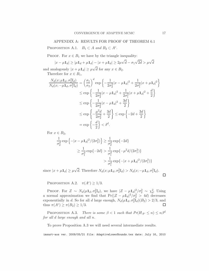
APPENDIX A: RESULTS FOR PROOF OF THEOREM 6.1
Proposition A.1. B1 ⊂ A and B2 ⊂ Ac.
Proof. For x ∈ B1 we have by the triangle inequality:
|x− µ1d| ≥ |µ1d + µ1d| − |x+ µ1d| ≥ 2µ√d− σ1
√2d > µ
√d
and analogously |x+ µ1d| ≥ µ√d for any x ∈ B2.
Therefore for x ∈ B1,
Nd(x;µ1d, σ22Id)
Nd(x;−µ1d, σ21Id)
=
(
σ1
σ2
)d
exp
{
− 1
2σ22
|x− µ1d|2 +1
2σ21
|x+ µ1d|2}
≤ exp
{
− 1
2σ22
|x− µ1d|2 +1
2σ21
|x+ µ1d|2 +d
2
}
≤ exp
{
− 1
2σ22
|x− µ1d|2 +3d
2
}
≤ exp
{
−µ2d
2σ22
+3d
2
}
≤ exp
{
−2d+3d
2
}
= exp
{
−d2
}
< δd.
For x ∈ B2,
1
σd2
exp{
−|x− µ1d|2/(2σ22)}
≥ 1
σd2
exp{−2d}
≥ 1
σd1
exp{−2d} > 1
σd1
exp{−µ2d/(2σ21)}
>1
σd1
exp{−|x+ µ1d|2/(2σ21)}
since |x+ µ1d| ≥ µ√d. Therefore Nd(x;µ1d, σ
22Id) > Nd(x;−µ1d, σ
21Id).
Proposition A.2. π(Ac) ≥ 1/3.
Proof. For Z ∼ Nd(µ1d, σ22Id), we have |Z − µ1d|2/σ2
2 ∼ χ2d. Using
a normal approximation we find that Pr(|Z − µ1d|2/σ22 > 4d) decreases
exponentially in d. So for all d large enough, Nd(µ1d, σ22Id)(B2) > 2/3, and
thus π(Ac) ≥ π(B2) ≥ 1/3.
Proposition A.3. There is some β < 1 such that Pr(HAc ≤ n) ≤ nβd
for all d large enough and all n.
To prove Proposition A.3 we will need several intermediate results.
imsart-aos ver. 2009/05/21 file: AdaptiveLowerBounds.tex date: July 16, 2010
18 SCHMIDLER & WOODARD
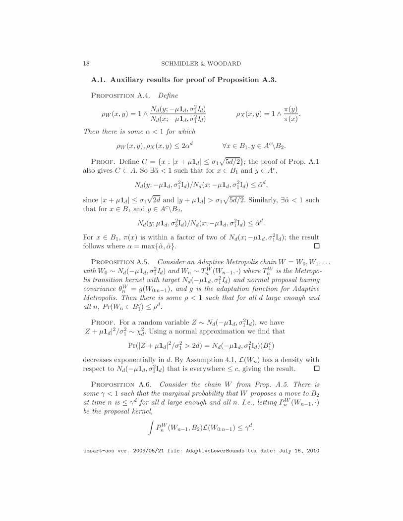
A.1. Auxiliary results for proof of Proposition A.3.
Proposition A.4. Define
ρW (x, y) = 1 ∧ Nd(y;−µ1d, σ21Id)
Nd(x;−µ1d, σ21Id)
ρX(x, y) = 1 ∧ π(y)
π(x).
Then there is some α < 1 for which
ρW (x, y), ρX (x, y) ≤ 2αd ∀x ∈ B1, y ∈ Ac\B2.
Proof. Define C = {x : |x + µ1d| ≤ σ1
√
5d/2}; the proof of Prop. A.1also gives C ⊂ A. So ∃α < 1 such that for x ∈ B1 and y ∈ Ac,
Nd(y;−µ1d, σ21Id)/Nd(x;−µ1d, σ
21Id) ≤ αd,
since |x + µ1d| ≤ σ1
√2d and |y + µ1d| > σ1
√
5d/2. Similarly, ∃α < 1 suchthat for x ∈ B1 and y ∈ Ac\B2,
Nd(y;µ1d, σ22Id)/Nd(x;−µ1d, σ
21Id) ≤ αd.
For x ∈ B1, π(x) is within a factor of two of Nd(x;−µ1d, σ21Id); the result
follows where α = max{α, α}.
Proposition A.5. Consider an Adaptive Metropolis chain W = W0,W1, . . .with W0 ∼ Nd(−µ1d, σ
21Id) and Wn ∼ TW
n (Wn−1, ·) where TWn is the Metropo-
lis transition kernel with target Nd(−µ1d, σ21Id) and normal proposal having
covariance θWn = g(W0:n−1), and g is the adaptation function for Adaptive
Metropolis. Then there is some ρ < 1 such that for all d large enough andall n, Pr(Wn ∈ Bc
1) ≤ ρd.
Proof. For a random variable Z ∼ Nd(−µ1d, σ21Id), we have
|Z + µ1d|2/σ21 ∼ χ2
d. Using a normal approximation we find that
Pr(|Z + µ1d|2/σ21 > 2d) = Nd(−µ1d, σ
21Id)(B
c1)
decreases exponentially in d. By Assumption 4.1, L(Wn) has a density withrespect to Nd(−µ1d, σ
21Id) that is everywhere ≤ c, giving the result.
Proposition A.6. Consider the chain W from Prop. A.5. There issome γ < 1 such that the marginal probability that W proposes a move to B2
at time n is ≤ γd for all d large enough and all n. I.e., letting PWn (Wn−1, ·)
be the proposal kernel,∫
PWn (Wn−1, B2)L(W0:n−1) ≤ γd.
imsart-aos ver. 2009/05/21 file: AdaptiveLowerBounds.tex date: July 16, 2010
CONVERGENCE OF ADAPTIVE MCMC 19
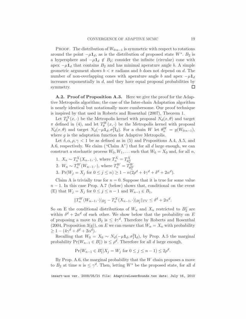
Proof. The distribution ofW0:n−1 is symmetric with respect to rotationsaround the point −µ1d, as is the distribution of proposed state W ∗. B2 isa hypersphere and −µ1d 6∈ B2; consider the infinite (circular) cone withapex −µ1d that contains B2 and has minimal aperature angle b. A simplegeometric argument shows b < π radians and b does not depend on d. Thenumber of non-overlapping cones with aperature angle b and apex −µ1d
increases exponentially in d, and they have equal proposal probabilities bysymmetry.
A.2. Proof of Proposition A.3. Here we give the proof for the Adap-tive Metropolis algorithm; the case of the Inter-chain Adaptation algorithmis nearly identical but notationally more cumbersome. Our proof techniqueis inspired by that used in Roberts and Rosenthal (2007), Theorem 1.
Let TXθ (x, ·) be the Metropolis kernel with proposal Nd(x, θ) and target
π defined in (4), and let TWθ (x, ·) be the Metropolis kernel with proposal
Nd(x, θ) and target Nd(−µ1d, σ21Id). For a chain W let θW
n = g(W0:n−1),where g is the adaptation function for Adaptive Metropolis.
Let δ, α, ρ, γ < 1 be as defined as in (5) and Propositions A.4, A.5, andA.6, respectively. We claim (“Claim A”) that for all d large enough, we canconstruct a stochastic process W0,W1, . . . such that W0 = X0 and, for all n,
1. Xn ∼ TXn (Xn−1, ·), where TX
n = TXθXn
2. Wn ∼ TWn (Wn−1, ·), where TW
n = TWθWn
3. Pr(Wj = Xj for 0 ≤ j ≤ n) ≥ 1 − n(2ρd + 4γd + δd + 2αd).
Claim A is trivially true for n = 0. Suppose that it is true for some valuen − 1. In this case Prop. A.7 (below) shows that, conditional on the event(E) that Wj = Xj for 0 ≤ j ≤ n− 1 and Wn−1 ∈ B1,
‖TWn (Wn−1, ·)|Bc
2− TX
n (Xn−1, ·)|Bc2‖TV ≤ δd + 2αd.
So on E the conditional distributions of Wn and Xn restricted to Bc2 are
within δd + 2αd of each other. We show below that the probability on Eof proposing a move to B2 is ≤ 4γd. Therefore by Roberts and Rosenthal(2004, Proposition 3(g)), on E we can ensure that Wn = Xn with probability≥ 1 − (4γd + δd + 2αd).
Recalling that W0 = X0 ∼ Nd(−µ1d, σ21Id), by Prop. A.5 the marginal
probability Pr(Wn−1 ∈ Bc1) is ≤ ρd. Therefore for all d large enough,
Pr(Wn−1 ∈ Bc1|Xj = Wj for 0 ≤ j ≤ n− 1) ≤ 2ρd.
By Prop. A.6, the marginal probability that the W chain proposes a moveto B2 at time n is ≤ γd. Then, letting W ∗ be the proposed state, for all d
imsart-aos ver. 2009/05/21 file: AdaptiveLowerBounds.tex date: July 16, 2010
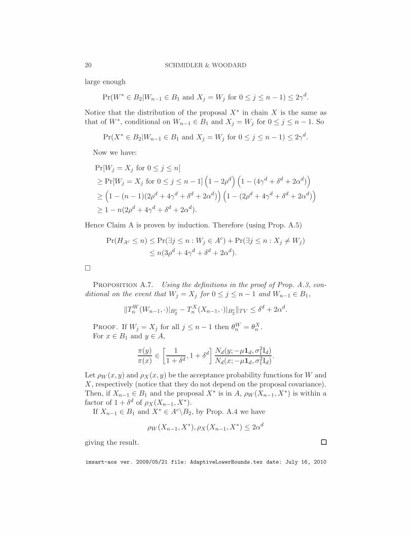
20 SCHMIDLER & WOODARD
large enough
Pr(W ∗ ∈ B2|Wn−1 ∈ B1 and Xj = Wj for 0 ≤ j ≤ n− 1) ≤ 2γd.
Notice that the distribution of the proposal X∗ in chain X is the same asthat of W ∗, conditional on Wn−1 ∈ B1 and Xj = Wj for 0 ≤ j ≤ n− 1. So
Pr(X∗ ∈ B2|Wn−1 ∈ B1 and Xj = Wj for 0 ≤ j ≤ n− 1) ≤ 2γd.
Now we have:
Pr[Wj = Xj for 0 ≤ j ≤ n]
≥ Pr[Wj = Xj for 0 ≤ j ≤ n− 1](
1 − 2ρd) (
1 − (4γd + δd + 2αd))
≥(
1 − (n− 1)(2ρd + 4γd + δd + 2αd)) (
1 − (2ρd + 4γd + δd + 2αd))
≥ 1 − n(2ρd + 4γd + δd + 2αd).
Hence Claim A is proven by induction. Therefore (using Prop. A.5)
Pr(HAc ≤ n) ≤ Pr(∃j ≤ n : Wj ∈ Ac) + Pr(∃j ≤ n : Xj 6= Wj)
≤ n(3ρd + 4γd + δd + 2αd).
�
Proposition A.7. Using the definitions in the proof of Prop. A.3, con-ditional on the event that Wj = Xj for 0 ≤ j ≤ n− 1 and Wn−1 ∈ B1,
‖TWn (Wn−1, ·)|Bc
2− TX
n (Xn−1, ·)|Bc2‖TV ≤ δd + 2αd.
Proof. If Wj = Xj for all j ≤ n− 1 then θWn = θX
n .For x ∈ B1 and y ∈ A,
π(y)
π(x)∈[
1
1 + δd, 1 + δd
]
Nd(y;−µ1d, σ21Id)
Nd(x;−µ1d, σ21Id)
.
Let ρW (x, y) and ρX(x, y) be the acceptance probability functions for W andX, respectively (notice that they do not depend on the proposal covariance).Then, if Xn−1 ∈ B1 and the proposal X∗ is in A, ρW (Xn−1,X
∗) is within afactor of 1 + δd of ρX(Xn−1,X
∗).If Xn−1 ∈ B1 and X∗ ∈ Ac\B2, by Prop. A.4 we have
ρW (Xn−1,X∗), ρX(Xn−1,X
∗) ≤ 2αd
giving the result.
imsart-aos ver. 2009/05/21 file: AdaptiveLowerBounds.tex date: July 16, 2010
CONVERGENCE OF ADAPTIVE MCMC 21
APPENDIX B: PROOF THAT π(A) > B FOR THE POTTS MODEL
Letting σ(z) = (σ1(z), . . . , σq(z)) denote the sufficient statistic vectorσk(z) =
∑
i 1(zi = k), we have
π(z) ∝ exp
{
α
2M
q∑
k=1
σk(z)2}
and the marginal distribution of σ is given by
ρ(σ) ∝(
M
σ1, . . . , σq
)
exp
{
α
2M
q∑
k=1
σ2k
}
.
For q ≥ 3 the critical value of the interaction parameter is αc = 2(q−1) ln(q−1)q−2 .
Using Stirling’s formula, Gore and Jerrum (1999) write( Mσ1,...,σq
)
in terms of
a = (a1, . . . , aq) = σ/M (the proportion of sites in each color):
(
M
σ1, . . . , σq
)
= exp
{
−Mq∑
k=1
ak ln ak + ∆(a)
}
where ∆(a) satisfies supa
|∆(a)| = O(lnM), and apply this to obtain:
ρ(σ) ∝ exp {fα(a)M + ∆(a)} where fα(a) =q∑
k=1
[
α
2a2
k − ak ln ak
]
Note fα does not depend on M , and for α > αc has global maxima at
permutations of a =(
x, 1−xq−1 , . . . ,
1−xq−1
)
for some x ∈[
q−1q , 1
)
(Gore and
Jerrum, 1999; Woodard et al., 2009b).
Consider subsets Ai ={
z : σi(z) >M2
}
, and observe that when q = 3
we have π(A1) = π(A2) = π(A3) by symmetry. The distribution π con-centrates near the global maxima of fα, in the sense that for any ǫ > 0,Pr{mins∈S3 ‖a(z) − sa‖2 < ǫ} → 1 as M → ∞ (Gore and Jerrum, 1999),where S3 is the symmetric group of 3 elements. If mins∈S3 ‖a(z)−sa‖2 < 1/6then z ∈ A1 ∪ A2 ∪ A3, so π(A1 ∪ A2 ∪ A3) → 1 as M → ∞, and there issome M∗ such that π(A1) ≥ 1
4 for M > M∗. For q > 3, the same argumentyields some M∗∗ such that π(A) ≥ 1
q+1 for M > M∗∗.
REFERENCES
Aldous, D. (1982), “Some inequalities for reversible Markov chains,” Journal of the LondonMathematical Society, 25, 564–576.
imsart-aos ver. 2009/05/21 file: AdaptiveLowerBounds.tex date: July 16, 2010
22 SCHMIDLER & WOODARD
Andrieu, C., and Atchade, Y. F. (2007), “On the efficiency of adaptive MCMC algorithms,”Electronic Communications in Probability, 12, 336–349.
Andrieu, C., and Moulines, E. (2006), “On the ergodicity properties of some adaptiveMCMC algorithms,” Annals of Applied Probability, 16, 1462–1505.
Andrieu, C., and Roberts, G. O. (2009), “The Pseudo-Marginal Approach for EfficientMonte Carlo Computations,” Annals of Statistics, 37(2), 697–725.
Atchade, Y. F. (2009a), “A cautionary tale on the efficiency of some adaptive Monte Carloschemes,” Annals of Applied Probability, . Accepted.
Atchade, Y. F. (2009b), “Resampling from the past to improve on MCMC algorithms,”Far East Journal of Theoretical Probability, 27, 81–99.
Bhatnagar, N., and Randall, D. (2004), Torpid mixing of simulated tempering on the Pottsmodel,, in Proceedings of the 15th ACM/SIAM Symposium on Discrete Algorithms,pp. 478–487.
Binder, K., and Heermann, D. W. (2002), Monte Carlo Simulation in Statistical Physics,4th edn Springer.
Craiu, R. V., Rosenthal, J., and Yang, C. (2009), “Learn from thy neighbor: Parallel-chainand regional adaptive MCMC,” Journal of the American Statistical Association, . Inpress.
Douc, R., Guillin, A., Marin, J., and Robert, C. P. (2007), “Convergence of AdaptiveMixtures of Importance Sampling Schemes,” Annals of Statistics, 35(1), 420–448.
Flegal, J. M. (2008), “Markov Chain Monte Carlo: Can We Trust the Third SignificantFigure?,” Statistical Science, 23(2), 250–260.
Frieze, A., Kannan, R., and Polson, N. (1994), “Sampling from log-concave distributions,”Annals of Applied Probability, 4, 812–837.
Gelfand, A. E., and Sahu, S. K. (1994), “On Markov chain Monte Carlo acceleration,”Journal of Computational and Graphical Statistics, 3, 261–276.
Geman, S., and Geman, D. (1984), “Stochastic relaxation, Gibbs distributions, and theBayesian restoration of images,” IEEE Transactions on Pattern Analysis and MachineIntelligence, 6, 721–741.
Geyer, C. J. (1991), Markov chain Monte Carlo maximum likelihood,, in Computing Sci-ence and Statistics, Volume 23: Proceedings of the 23rd Symposium on the Interface, ed.E. Keramidas, Interface Foundation of North America, Fairfax Station, VA, pp. 156–163.
Geyer, C. J., and Thompson, E. A. (1995), “Annealing Markov chain Monte Carlo withapplications to ancestral inference,” Journal of the American Statistical Association,90, 909–920.
Gore, V. K., and Jerrum, M. R. (1999), “The Swendsen-Wang process does not alwaysmix rapidly,” J. of Statist. Physics, 97, 67–85.
Green, P. J., and Richardson, S. (2002), “Hidden Markov models and disease mapping,”Journal of the American Statistical Association, 97, 1055–1070.
Haario, H., Saksman, E., and Tamminen, J. (2001), “An adaptive Metropolis algorithm,”Bernoulli, 7, 223–242.
Heaton, M., and Schmidler, S. C. (2009), A Multiscale Adaptive MCMC Algorithm,.(submitted).
Ji, C., and Schmidler, S. C. (2009), “Adaptive Markov chain Monte Carlo for BayesianVariable Selection,” Journal of Computational and Graphical Statistics, (to appear).
Jones, G. L., and Hobert, J. P. (2001), “Honest Exploration of Intractable ProbabilityDistributions via Markov Chain Monte Carlo,” Statistical Science, 16(4), 312–334.
Kou, S. C., Zhou, Q., and Wong, W. H. (2006), “Equi-Energy Sampler with Applicationsin Statistical Inference and Statistical Mechanics,” Annals of Statistics, 34, 1581–1619.
imsart-aos ver. 2009/05/21 file: AdaptiveLowerBounds.tex date: July 16, 2010
CONVERGENCE OF ADAPTIVE MCMC 23
Lawler, G. F., and Sokal, A. D. (1988), “Bounds on the L2 spectrum for Markov chains
and Markov processes: a generalization of Cheeger’s inequality,” Transactions of theAmerican Mathematical Society, 309, 557–580.
Liang, F., and Wong, W. H. (1999), “Dynamics Weighting in Simulatinos of Spin Systems,”PhysLettA, 252, 257–262.
Liu, J. S., Liang, F., and Wong, W. H. (2001), “A Theory for Dynamics Weighting in MonteCarlo Computation,” Journal of the American Statistical Association, 96(454), 561–573.
Madras, N., ed (2000), Fields Institute Communications Volume 26: Monte Carlo Methods,Providence, RI: American Mathematical Society.
Marinari, E., and Parisi, G. (1992), “Simulated tempering: a new Monte Carlo scheme,”Europhysics Letters, 19, 451–458.
Mengersen, K. L., and Tweedie, R. L. (1996), “Rates of Convergence of Hastings andMetropolis Algorithms,” Annals of Statistics, 24(1), 101–121.
Minary, P., and Levitt, M. (2006), “Discussion of ”Equi-energy sampler” by Kou, Zhou,and Wong,” Annals of Statistics, 34, 1636–1641.
Mira, A. (2001), “Ordering and Improving the Performance of Monte Carlo MarkovChains,” Statistical Science, 16(4), 340–350.
Mira, A., and Geyer, C. J. (2000), “On Non-Reversible Markov Chains,”. In Madras(2000).
Neal, R. (2003), “Slice sampling (with discussion),” Annals of Statistics, 31, 705–767.Roberts, G. O., and Rosenthal, J. S. (2001), “Optimal Scaling for Various Metropolis-
Hastings Algorithms,” Statistical Science, 16(4), 351–367.Roberts, G. O., and Rosenthal, J. S. (2004), “General state space Markov chains and
MCMC algorithms,” Probability Surveys, 1, 20–71.Roberts, G. O., and Rosenthal, J. S. (2007), “Coupling and Ergodicity of Adaptive
MCMC,” Journal of Applied Probability, 44, 458–475.Schmidler, S. C., and Woodard, D. B. (2009), Computational complexity and Bayesian
analysis,. In preparation.Sinclair, A. (1992), “Improved bounds for mixing rates of Markov chains and multicom-
modity flow,” Combinatorics, Probability, and Computing, 1, 351–370.Tierney, L. (1994), “Markov Chains for Exploring Posterior Distributions,” Annals of
Statistics, 22(4), 1701–1728.Wang, F. G., and Landau, D. P. (2001), “Efficient, Multiple-Range Random Walk Algo-
rithm to Calculate the Density of States,” Physical Review Letters, 86(10), 2050–2053.Woodard, D. B., Schmidler, S. C., and Huber, M. (2009a), “Conditions for rapid mixing
of parallel and simulated tempering on multimodal distributions,” Annals of AppliedProbability, 19, 617–640.
Woodard, D. B., Schmidler, S. C., and Huber, M. (2009b), “Sufficient conditions for torpidmixing of parallel and simulated tempering,” Electronic Journal of Probability, 14, 780–804.
E-mail: [email protected] E-mail: [email protected]
Department of Statistical Science
Box 90251
Duke University
Durham, NC 27708-0251
E-mail: [email protected]: http://www.stat.duke.edu/∼scs
School of Operations Research and
Information Engineering
206 Rhodes Hall
Ithaca, NY
E-mail: [email protected]: http://people.orie.cornell.edu/∼woodard
imsart-aos ver. 2009/05/21 file: AdaptiveLowerBounds.tex date: July 16, 2010