CALIBRATING A HEC-RAS MODEL OF V-NOTCH WEIR AS …

CALIBRATING A HEC-RAS MODEL OF V-NOTCH WEIR AS INLINE

STRUCTURE USING OPEN CHANNEL FLUME FLOW METHOD AND ITS

APPLICATION FOR SEDIMENT TRANSPORT

RABIATUL ARBAIYAH BINTI RUSLAN

Report submitted in partial fulfilment of the requirements

for the award of the degree of

B.Eng (Hons.) of Civil Engineering

Faculty of Civil Engineering and Earth Resources

UNIVERSITI MALAYSIA PAHANG

JUNE 2015

vi

ABSTRACT

The Hydrologic Engineering Center’s River Analysis System (HEC- RAS) is a one-

dimensional computer model intended to perform hydraulic calculations for a network

of open channels. This model is widely available, free of cost and the most commonly

used hydraulic model in the United States. Most HEC-RAS models are steady state.

Unsteady flow analysis in HEC-RAS differs in many ways from the traditional steady

state analysis. The main objective of this study is to compare the results of the water

surface profile between HEC-RAS and the laboratory experiment. The procedure and

methodology to collect the data are described. HEC-RAS will determine the water

surface profile with three different discharge and manning value. The data is collected

along the flume with V-notch weir is placed at fixed point. After the laboratory work is

done, the computational work will obtained the result and the comparison is made.

HEC-RAS’s result will determine whether it is reliable to use. The prediction of

sediment transport in the upstream is determined in this study. From the result and

discussion the appropriate manning value is 0.010 s/m1/3

with the value of root mean

square error of 0.026358m from the upstream. The sediment transport is occur at the

upstream. This research can be conclude that HEC-RAS is reliable to be used.

vii

ABSTRAK

Hydrologic Engineering Center’s River Analysis System (HEC- RAS) adalah model

komputer satu dimensi yang bertujuan untuk melakukan pengiraan hidraulik untuk

rangkaian saluran terbuka. Model ini boleh didapati secara meluas, bebas daripada kos

dan model yang paling biasa digunakan hidraulik di Amerika Syarikat. Kebanyakan

model HEC-RAS adalah keadaan mantap. Analisis aliran tak mantap dalam HEC-RAS

banyak berbeza daripada analisis keadaan mantap tradisional. Objektif utama kajian ini

adalah untuk membandingkan keputusan profil permukaan air di antara HEC-RAS dan

eksperimen makmal. Prosedur dan kaedah untuk mengumpul data adalah seperti yang

dinyatakan. HEC-RAS akan menentukan profil permukaan air dengan tiga pelepasan

yang berbeza dan nilai pengendalian. Data yang dikumpul sepanjang flum dengan

empang V-takuk diletakkan pada titik tetap. Selepas kerja-kerja makmal yang

dilakukan, kerja-kerja pengkomputeran akan mendapat keputusan dan perbandingan itu

dibuat. Hasil HEC-RAS akan menentukan sama ada ia boleh dipercayai untuk

digunakan. Ramalan pengangkutan sedimen di hulu yang ditentukan dalam kajian ini.

Dari hasil dan perbincangan nilai pengendalian yang sesuai adalah 0.010 s/m1/3

dengan

nilai punca min kuasa dua ralat 0.026358m dari hulu. Pengangkutan sedimen adalah

berlaku di hulu. Kajian ini boleh membuat kesimpulan bahawa HEC-RAS boleh

dipercayai yang akan digunakan.

viii

TABLE OF CONTENT

SUPERVISOR’S DECLARATION ii

STUDENT’S DECLARATION iii

DEDICATIONS iv

ACKNOWLEDGEMENTS v

ABSTRACT vi

ABSTRAK vii

TABLE OF CONTENTS viii

LIST OF TABLES x

LIST OF FIGURES xi

LIST OF SYMBOLS xiv

CHAPTER 1 INTRODUCTION

1.1 Introduction 1

1.2 Background of Study 1

1.3 Problem Statement 2

1.4 Objectives 2

1.5 Scope of Study 2

1.6 Research Significance 3

CHAPTER 2 LITERATURE REVIEW

2.1 Introduction 4

2.2 Open channel flume hydraulic 4

2.2.1 Manning equation

2.2.2 Manning Roughness Coefficient

2.2.3 Flume and V-Notch Weir

2.2.4 Hydraulic Jump

2.2.5 Froude Number

2.2.6 Water Surface Profile

5

6

10

11

12

14

2.3 HEC-RAS 16

2.3.1 Unsteady flow

2.3.2 Root mean square error

2.3.3 Finite difference approximation

2.3.4 Sediment transport

17

18

18

19

ix

CHAPTER 3 RESEARCH METHODOLOGY

3.1 Introduction 21

3.2 Research design 21

3.3 Flow chart of project methodology 21

3.4 Laboratory work 23

3.5 Computational work

3.5.1 Geometric Data


25

25

28

3.6 Analyze result 28

CHAPTER 4 RESULT ANALYSIS AND DISCUSSION

4.1 Introduction 29

4.2 Result and discussion 29

4.2.1 Laboratory experiment result

4.2.2 HEC-RAS result

4.2.3 Root mean square error


30

33

36

46

CHAPTER 5 CONCLUSION AND RECOMMENDATIONS

5.1 Conclusion 47

5.2 Recommendations 48

REFERENCES 49

APPENDICES 50

x

LIST OF TABLES

Table No. Title Page

2.1 Manning roughness coefficient

7

2.2 Classification of hydraulic jumps according to Froude Number

13

2.3 Description of hydraulic curve

14

2.4 Description of Froude number

15

2.5 Non-transported sediment: Bed material

19

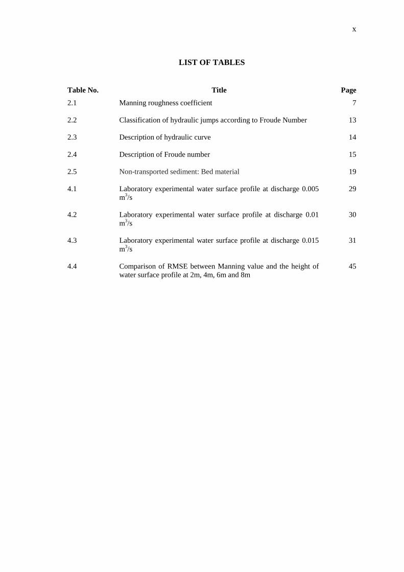
4.1 Laboratory experimental water surface profile at discharge 0.005

m3/s

29


m3/s

30


m3/s

31

4.4 Comparison of RMSE between Manning value and the height of

water surface profile at 2m, 4m, 6m and 8m

45

xi

LIST OF FIGURES

Figure No. Title Page

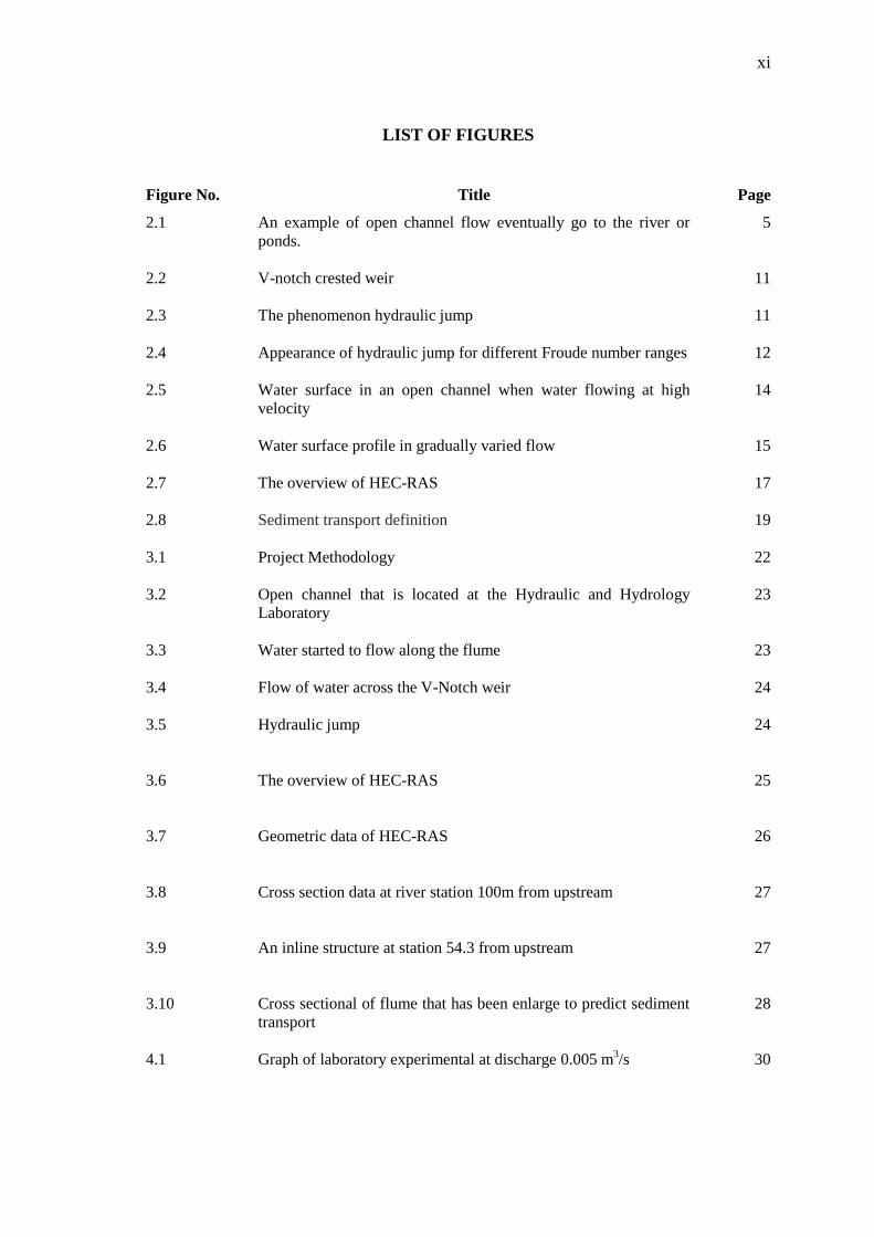
2.1 An example of open channel flow eventually go to the river or

ponds.

5

2.2 V-notch crested weir

11

2.3 The phenomenon hydraulic jump

11

2.4 Appearance of hydraulic jump for different Froude number ranges

12

2.5 Water surface in an open channel when water flowing at high

velocity

14

2.6 Water surface profile in gradually varied flow

15

2.7 The overview of HEC-RAS

17

2.8 Sediment transport definition

19

3.1 Project Methodology

22

3.2 Open channel that is located at the Hydraulic and Hydrology

Laboratory

23

3.3 Water started to flow along the flume

23

3.4 Flow of water across the V-Notch weir

24

3.5 Hydraulic jump

24

3.6 The overview of HEC-RAS

25

3.7 Geometric data of HEC-RAS

26

3.8 Cross section data at river station 100m from upstream

27

3.9 An inline structure at station 54.3 from upstream

27

3.10 Cross sectional of flume that has been enlarge to predict sediment

transport

28

4.1 Graph of laboratory experimental at discharge 0.005 m3/s

30

xii

4.3 Graph of laboratory experimental at discharge 0.015 m3/s

32

4.4 Comparison of water surface profile between HEC-RAS and

Laboratory Experiment with the discharge of 0.015 m3/s with the

Manning value of 0.010 s/m1/

33



Manning value of 0.010 s/m1/3

34



Manning value of 0.010 s/m1/3

35

4.7 The height of the water surface profile against discharge when the

Manning value is 0.009 s/m1/3

at 2m from upstream

36



at 4m from upstream

37



at 6m from upstream

37



at 8m from upstream

38



at 10m from upstream

38



at 2m from upstream

39



at 4m from upstream

40



at 6m from upstream

40



at 8m from upstream

41




41



at 2m from upstream

42



at 4m from upstream

43



at 6m from upstream

43

xiii



at 8m from upstream

44




44

4.22 Sediment transport occurs at the upstream 46

xiv

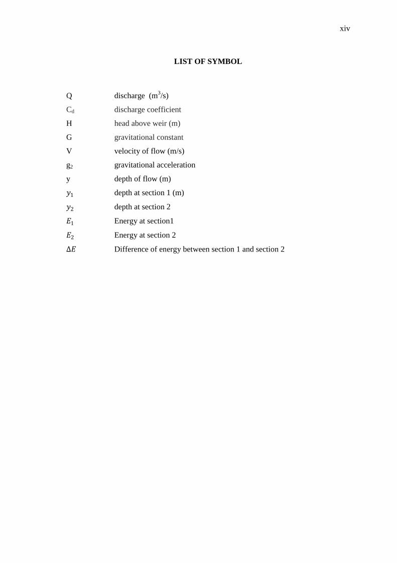
LIST OF SYMBOL

Q discharge (m3/s)

Cd discharge coefficient

H head above weir (m)

G gravitational constant

V velocity of flow (m/s)

g2 gravitational acceleration

y depth of flow (m)

𝑦1 depth at section 1 (m)

𝑦2 depth at section 2

𝐸1 Energy at section1

𝐸2 Energy at section 2

∆𝐸 Difference of energy between section 1 and section 2

CHAPTER 1

INTRODUCTION

1.1 INTRODUCTION

The Hydrologic Engineering Center’s River Analysis System (HEC- RAS) is a

one-dimensional computer model intended to perform hydraulic calculations for a

network of open channels. This model is widely available, free of cost and the most

commonly used hydraulic model in the United States. Most HEC-RAS models are

steady state. Unsteady flow analysis in HEC-RAS differs in many ways from the

traditional steady state analysis. The largest difference involves the ability to input a full

hydrograph to analyze the response of the river system to flows that vary with time.

1.2 BACKGROUND OF STUDY

Manning value plays an important role in river analysis. It will determine the

flow of the water and also the height of the water surface profile. The complex nature of

the flow, standard hydraulic modeling tools, such as HEC-RAS program, could not be

used accurately to determine the flow.

Laboratory experiment is carried out to compare the result of the HEC-RAS

program. Prediction of sediment transport using HEC-RAS to determine whether there

is transport in the inline structure.

2

1.3 PROBLEM STATEMENT

HEC-RAS have been used for almost 20 years and up till today HEC-RAS has

difficulty in the stimulation of a steep channel or stream. Besides that, many users

around the world find instability numerical unsteady flow. It is 1 dimensional

hydrodynamic modeling and might not be able to work well in multi-dimensioning

modeling. HEC-RAS is used to stimulate Tawau design spillway design and it is found

that the results obtained in the hydraulic jump and water surface profile does not same

as in manual calculation.

1.4 OBJECTIVES

The objectives of this research are:

i. To determine the water surface profile height at upstream of V-notch weir

by using different.

ii. To compare the results of the water surface profile height between HEC-

RAS and laboratory experimental.

iii. To obtain the appropriate manning value.

iv. To predict the sediment transport pattern in the upstream of V-notch weir.

1.5 SCOPE OF STUDY

A prototype model of an open channel is constructed in laboratory for testing

purpose. The water flow through the V-notch weir model indicates the actual flow of

water from the reservoir. Study scopes that have been fixed are:

i. Experiment is conducted in Hydraulic & Hydrology Laboratory of Faculty of

Civil Engineering & Earth Resources, Universiti Malaysia Pahang.

ii. The model structure associated with a V-notch weir.

iii. Take into account of various water discharge and Manning value.

3

Once experiment conducted, the result will be compared with the HEC-RAS. In

addition, HEC-RAS will determine the sediment transport in the upstream.

1.6 RESARCH SIGNIFICANCE

HEC-RAS is an important tool for engineers to make decisions and to stimulate

the design. It is widely used by the engineers around the world for steady flow water

surface profile computation, unsteady flow simulation, movable boundary sediment

transport computation and water quality analysis. Besides that, this software is freely

distributed which make it more people using it. The comparison between HEC-RAS

and laboratory experiment is used to determine the accuracy of the manning value.

HEC-RAS also provide the other utilities such as one dimensional Quasi-Unsteady

Sediment Transport and to predict whether there is sediment transport in the inline

structure.

CHAPTER 2

LITERATURE REVIEW

2.1 INTRODUCTION

This chapter will divided into two parts. First part is the open channel. It will

subdivide into manning equation, hydraulic jump, flume and v-notch weir, Froude

number and water surface profile. Second part is HEC-RAS. It will subdivide into Root

Mean Square Error, Finite Difference Method and sediment transport.

2.2 OPEN CHANNEL

Open channel flow can be said to be as the flow of fluid (water) over the deep

hollow surface (channel) with the cover of atmosphere on the top. Examples of open

channels flow are river, streams, flumes, sewers, ditches and lakes etc. we can be said to

be as open channel is a way for flow of fluid having pressure equal to the atmospheric

pressure. While on the other hand flow under pressure is said to be as pipe flow. In

example, flow of fluid through the sewer pipes.

Open-channel flow is usually categorized on the basis of steadiness. Flow is said

to be steady when the velocity at any point of observation does not change with time; if

it changes from time to time, flow is said to be unsteady. At every instant, if the velocity

is the same at all points along the channel, flow is said to be uniform; if it is not the

same, flow is said to be non-uniform. Non-uniform flow which is also steady is called

as varied flow; non-uniform flow which is unsteady is called as variable flow. Flow

occurs from a higher to a lower concentration by aid of gravity. Another important

http://www.aboutcivil.org/open-channel-flows-definition-types-comparison.html

5

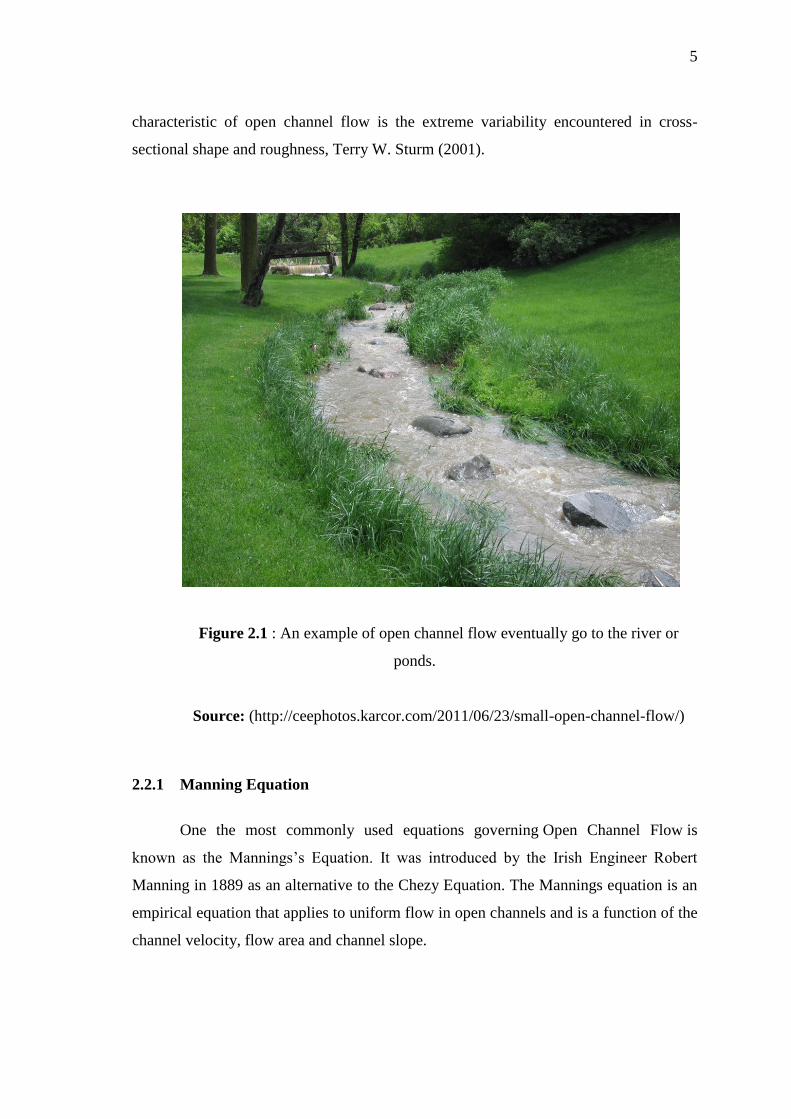
characteristic of open channel flow is the extreme variability encountered in cross-

sectional shape and roughness, Terry W. Sturm (2001).

Figure 2.1 : An example of open channel flow eventually go to the river or

ponds.

Source: (http://ceephotos.karcor.com/2011/06/23/small-open-channel-flow/)

2.2.1 Manning Equation

One the most commonly used equations governing Open Channel Flow is

known as the Mannings’s Equation. It was introduced by the Irish Engineer Robert

Manning in 1889 as an alternative to the Chezy Equation. The Mannings equation is an

empirical equation that applies to uniform flow in open channels and is a function of the

channel velocity, flow area and channel slope.

http://ceephotos.karcor.com/2011/06/23/small-open-channel-flow/

http://www.fsl.orst.edu/geowater/FX3/help/8_Hydraulic_Reference/Open_Channel_Flow.htm

6

It can also be used to calculate values of other uniform open channel flow

parameters such as channel slope. Manning roughness coefficient or normal depth,

when the water flow rate through the open channel is known. An example set of

calculations includes average flow velocity determination and water flow calculation for

a given channel and flow depth. The Manning equation applies to open channel flow in

natural channels as well as to man-made channels. For example, river discharge can be

related to the depth of water flow and river parameters like slope, width and cross-

sectional shape.

The Manning equation is:

𝑄 = 𝑉𝐴 =(1)𝐴𝑅

23 𝑆

𝑛

(2.1)

Where:

V= velocity (m/s)

A= flow area (m2)

R= hydraulic radius (m)

S= channel slope (m/m)

n= manning roughness coefficient

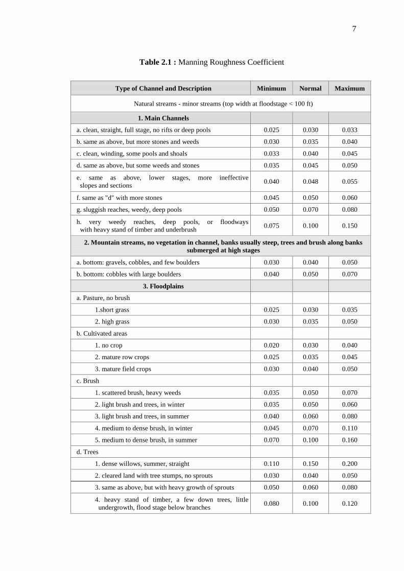
2.2.2 Manning Roughness Coefficient

The Manning roughness coefficient, n, is an experimentally determined

constant. It value depends depends upon the nature of the channel and its surface.

Tables giving values of n for different man-made and natural channel types and

surfaces are available in many textbooks, handbooks and on-line. The table below

gave by Chow (1959) an idea of variability to be expected in Manning’s, n. Manning

roughness coefficient values for several surfaces commonly used for open channel

flow. In general smoother surfaces have lower Manning roughness coefficient values

and rougher surfaces have higher Manning roughness coefficient values

.

7

Table 2.1 : Manning Roughness Coefficient

Type of Channel and Description Minimum Normal Maximum

Natural streams - minor streams (top width at floodstage < 100 ft)

1. Main Channels

a. clean, straight, full stage, no rifts or deep pools 0.025 0.030 0.033

b. same as above, but more stones and weeds 0.030 0.035 0.040

c. clean, winding, some pools and shoals 0.033 0.040 0.045

d. same as above, but some weeds and stones 0.035 0.045 0.050

e. same as above, lower stages, more ineffective

slopes and sections 0.040 0.048 0.055

f. same as "d" with more stones 0.045 0.050 0.060

g. sluggish reaches, weedy, deep pools 0.050 0.070 0.080

h. very weedy reaches, deep pools, or floodways

with heavy stand of timber and underbrush 0.075 0.100 0.150

2. Mountain streams, no vegetation in channel, banks usually steep, trees and brush along banks

submerged at high stages

a. bottom: gravels, cobbles, and few boulders 0.030 0.040 0.050

b. bottom: cobbles with large boulders 0.040 0.050 0.070

3. Floodplains

a. Pasture, no brush

1.short grass 0.025 0.030 0.035

2. high grass 0.030 0.035 0.050

b. Cultivated areas

1. no crop 0.020 0.030 0.040

2. mature row crops 0.025 0.035 0.045

3. mature field crops 0.030 0.040 0.050

c. Brush

1. scattered brush, heavy weeds 0.035 0.050 0.070

2. light brush and trees, in winter 0.035 0.050 0.060

3. light brush and trees, in summer 0.040 0.060 0.080

4. medium to dense brush, in winter 0.045 0.070 0.110

5. medium to dense brush, in summer 0.070 0.100 0.160

d. Trees

1. dense willows, summer, straight 0.110 0.150 0.200

2. cleared land with tree stumps, no sprouts 0.030 0.040 0.050

3. same as above, but with heavy growth of sprouts 0.050 0.060 0.080

4. heavy stand of timber, a few down trees, little

undergrowth, flood stage below branches 0.080 0.100 0.120

8

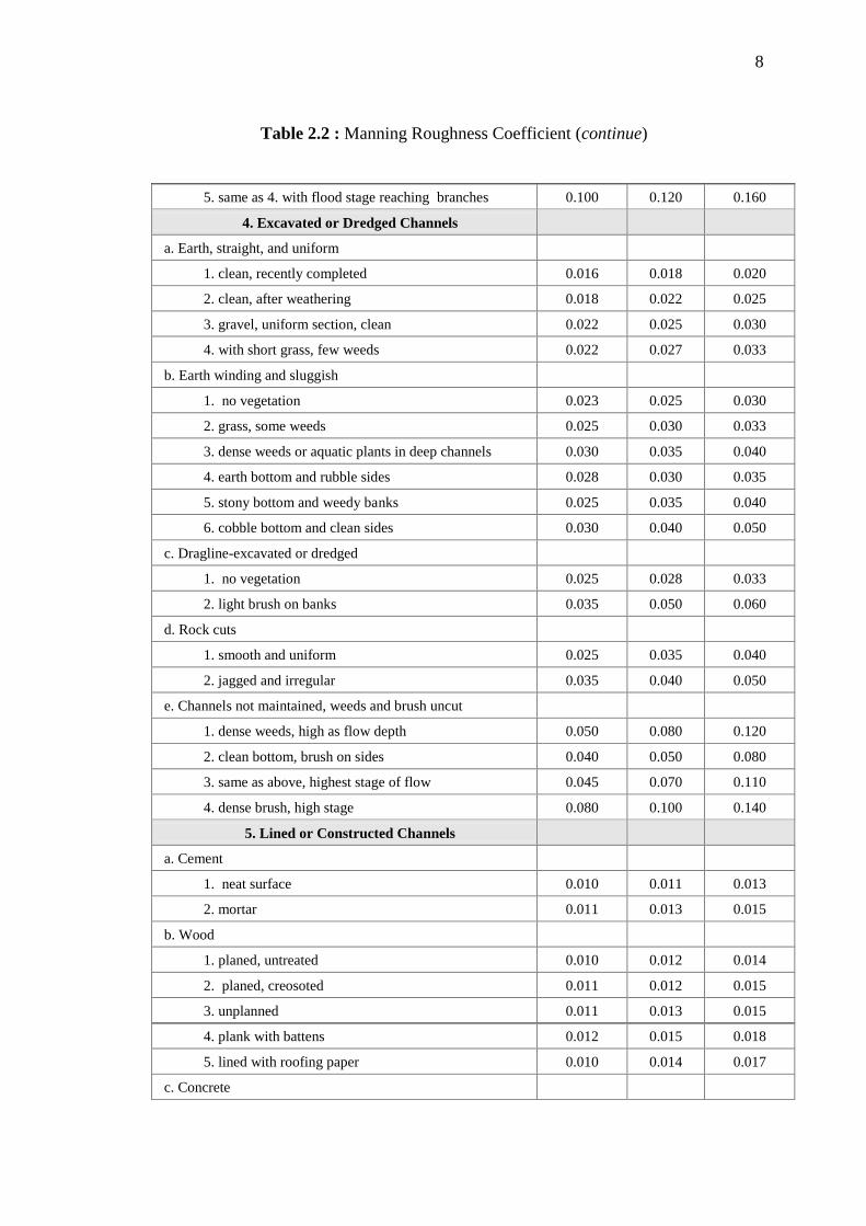
Table 2.2 : Manning Roughness Coefficient (continue)

5. same as 4. with flood stage reaching branches 0.100 0.120 0.160

4. Excavated or Dredged Channels

a. Earth, straight, and uniform

1. clean, recently completed 0.016 0.018 0.020

2. clean, after weathering 0.018 0.022 0.025

3. gravel, uniform section, clean 0.022 0.025 0.030

4. with short grass, few weeds 0.022 0.027 0.033

b. Earth winding and sluggish

1. no vegetation 0.023 0.025 0.030

2. grass, some weeds 0.025 0.030 0.033

3. dense weeds or aquatic plants in deep channels 0.030 0.035 0.040

4. earth bottom and rubble sides 0.028 0.030 0.035

5. stony bottom and weedy banks 0.025 0.035 0.040

6. cobble bottom and clean sides 0.030 0.040 0.050

c. Dragline-excavated or dredged

1. no vegetation 0.025 0.028 0.033

2. light brush on banks 0.035 0.050 0.060

d. Rock cuts

1. smooth and uniform 0.025 0.035 0.040

2. jagged and irregular 0.035 0.040 0.050

e. Channels not maintained, weeds and brush uncut

1. dense weeds, high as flow depth 0.050 0.080 0.120

2. clean bottom, brush on sides 0.040 0.050 0.080

3. same as above, highest stage of flow 0.045 0.070 0.110

4. dense brush, high stage 0.080 0.100 0.140

5. Lined or Constructed Channels

a. Cement

1. neat surface 0.010 0.011 0.013

2. mortar 0.011 0.013 0.015

b. Wood

1. planed, untreated 0.010 0.012 0.014

2. planed, creosoted 0.011 0.012 0.015

3. unplanned 0.011 0.013 0.015

4. plank with battens 0.012 0.015 0.018

5. lined with roofing paper 0.010 0.014 0.017

c. Concrete

9

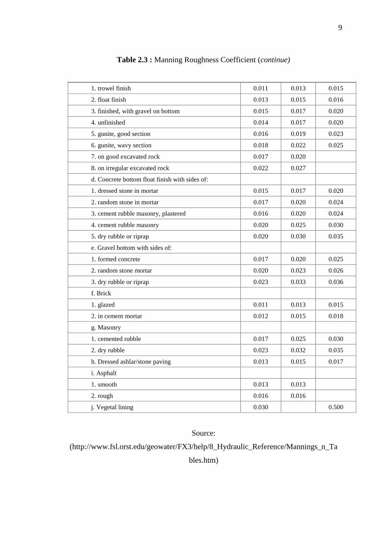
Table 2.3 : Manning Roughness Coefficient (continue)

1. trowel finish 0.011 0.013 0.015

2. float finish 0.013 0.015 0.016

3. finished, with gravel on bottom 0.015 0.017 0.020

4. unfinished 0.014 0.017 0.020

5. gunite, good section 0.016 0.019 0.023

6. gunite, wavy section 0.018 0.022 0.025

7. on good excavated rock 0.017 0.020

8. on irregular excavated rock 0.022 0.027

d. Concrete bottom float finish with sides of:

1. dressed stone in mortar 0.015 0.017 0.020

2. random stone in mortar 0.017 0.020 0.024

3. cement rubble masonry, plastered 0.016 0.020 0.024

4. cement rubble masonry 0.020 0.025 0.030

5. dry rubble or riprap 0.020 0.030 0.035

e. Gravel bottom with sides of:

1. formed concrete 0.017 0.020 0.025

2. random stone mortar 0.020 0.023 0.026

3. dry rubble or riprap 0.023 0.033 0.036

f. Brick

1. glazed 0.011 0.013 0.015

2. in cement mortar 0.012 0.015 0.018

g. Masonry

1. cemented rubble 0.017 0.025 0.030

2. dry rubble 0.023 0.032 0.035

h. Dressed ashlar/stone paving 0.013 0.015 0.017

i. Asphalt

1. smooth 0.013 0.013

2. rough 0.016 0.016

j. Vegetal lining 0.030

0.500

Source:

(http://www.fsl.orst.edu/geowater/FX3/help/8_Hydraulic_Reference/Mannings_n_Ta

bles.htm)

10

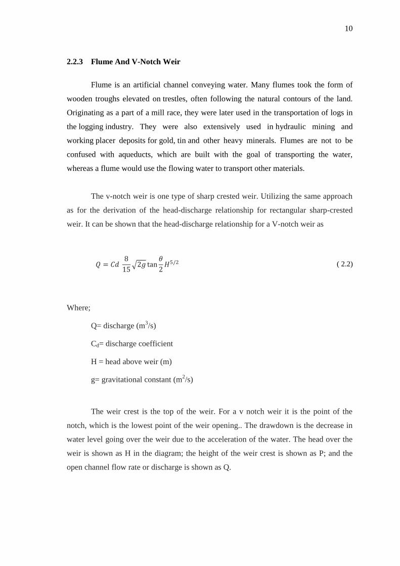
2.2.3 Flume And V-Notch Weir

Flume is an artificial channel conveying water. Many flumes took the form of

wooden troughs elevated on trestles, often following the natural contours of the land.

Originating as a part of a mill race, they were later used in the transportation of logs in

the logging industry. They were also extensively used in hydraulic mining and

working placer deposits for gold, tin and other heavy minerals. Flumes are not to be

confused with aqueducts, which are built with the goal of transporting the water,

whereas a flume would use the flowing water to transport other materials.

The v-notch weir is one type of sharp crested weir. Utilizing the same approach

as for the derivation of the head-discharge relationship for rectangular sharp-crested

weir. It can be shown that the head-discharge relationship for a V-notch weir as

𝑄 = 𝐶𝑑 8

15 2𝑔 tan

𝜃

2𝐻5/2

( 2.2)

Where;

Q= discharge (m3/s)

Cd= discharge coefficient

H = head above weir (m)

g= gravitational constant (m2/s)

The weir crest is the top of the weir. For a v notch weir it is the point of the

notch, which is the lowest point of the weir opening.. The drawdown is the decrease in

water level going over the weir due to the acceleration of the water. The head over the

weir is shown as H in the diagram; the height of the weir crest is shown as P; and the

open channel flow rate or discharge is shown as Q.

http://en.wikipedia.org/wiki/Trestle

http://en.wikipedia.org/wiki/Mill_race

http://en.wikipedia.org/wiki/Logging

http://en.wikipedia.org/wiki/Hydraulic_mining

http://en.wikipedia.org/wiki/Placer_deposit

http://en.wikipedia.org/wiki/Gold

http://en.wikipedia.org/wiki/Tin

11

Figure 2.2: V-notch crested weir

Source : (http://www.engineeringexcelspreadsheets.com/2011/04/v-notch-weir-

calculator-excel-spreadsheet/)

2.2.4 Hydraulic Jump

An Italian engineer, Bidone (1818) found that hydraulic jump is the

phenomenon when supercritical stream meets a subcritical stream of sufficient depth.

The supercritical stream jumps up to meet the alternate depth. The hydraulic jump

serves as an energy dissipater to dissipate the excess energy of flowing water

downstream of hydraulic structure.

Figure 2.3: The phenomenon hydraulic jump

Source : (krcproject.groups.et.byu.net)

12

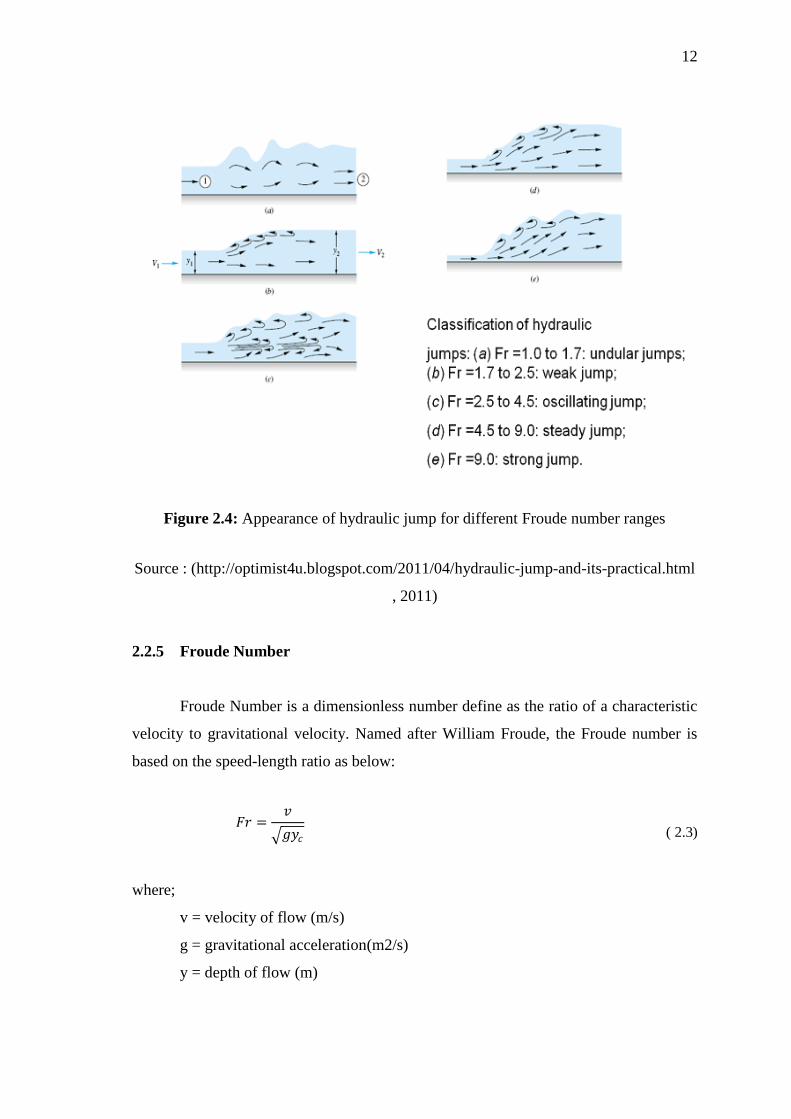
Figure 2.4: Appearance of hydraulic jump for different Froude number ranges

Source : (http://optimist4u.blogspot.com/2011/04/hydraulic-jump-and-its-practical.html

, 2011)

2.2.5 Froude Number

Froude Number is a dimensionless number define as the ratio of a characteristic

velocity to gravitational velocity. Named after William Froude, the Froude number is

based on the speed-length ratio as below:

𝐹𝑟 =𝑣

𝑔𝑦𝑐

( 2.3)

where;

v = velocity of flow (m/s)

g = gravitational acceleration(m2/s)

y = depth of flow (m)

http://optimist4u.blogspot.com/2011/04/hydraulic-jump-and-its-practical.html

13

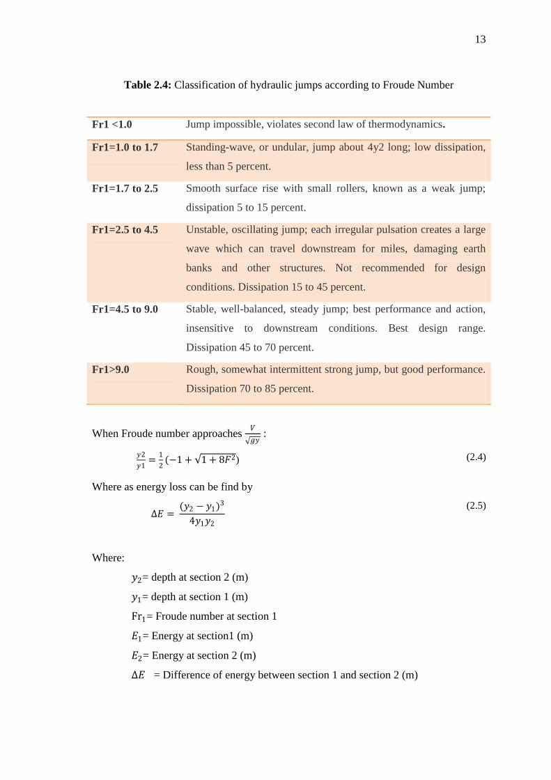
Table 2.4: Classification of hydraulic jumps according to Froude Number

Fr1 <1.0 Jump impossible, violates second law of thermodynamics.

Fr1=1.0 to 1.7 Standing-wave, or undular, jump about 4y2 long; low dissipation,

less than 5 percent.

Fr1=1.7 to 2.5 Smooth surface rise with small rollers, known as a weak jump;

dissipation 5 to 15 percent.

Fr1=2.5 to 4.5 Unstable, oscillating jump; each irregular pulsation creates a large

wave which can travel downstream for miles, damaging earth

banks and other structures. Not recommended for design

conditions. Dissipation 15 to 45 percent.

Fr1=4.5 to 9.0 Stable, well-balanced, steady jump; best performance and action,

insensitive to downstream conditions. Best design range.

Dissipation 45 to 70 percent.

Fr1>9.0 Rough, somewhat intermittent strong jump, but good performance.

Dissipation 70 to 85 percent.

When Froude number approaches 𝑉

𝑔𝑦 :

𝑦2

𝑦1=

1

2(−1 + 1 + 8𝐹2) (2.4)

Where as energy loss can be find by

∆𝐸 = (𝑦2 − 𝑦1)3

4𝑦1𝑦2

(2.5)

Where:

𝑦2= depth at section 2 (m)

𝑦1= depth at section 1 (m)

Fr1= Froude number at section 1

𝐸1= Energy at section1 (m)

𝐸2= Energy at section 2 (m)

∆𝐸 = Difference of energy between section 1 and section 2 (m)

14

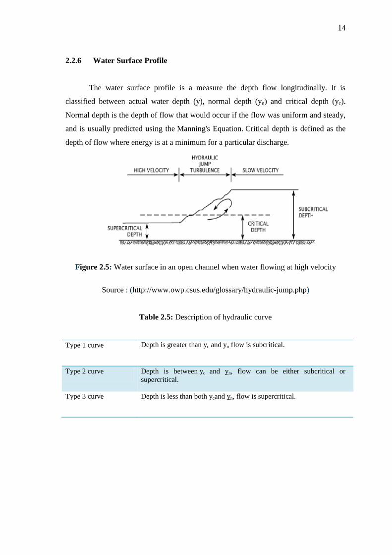
2.2.6 Water Surface Profile

The water surface profile is a measure the depth flow longitudinally. It is

classified between actual water depth (y), normal depth (yn) and critical depth (yc).

Normal depth is the depth of flow that would occur if the flow was uniform and steady,

and is usually predicted using the Manning's Equation. Critical depth is defined as the

depth of flow where energy is at a minimum for a particular discharge.

Figure 2.5: Water surface in an open channel when water flowing at high velocity

Source : (http://www.owp.csus.edu/glossary/hydraulic-jump.php)

Table 2.5: Description of hydraulic curve

Type 1 curve Depth is greater than yc and yn flow is subcritical.

Type 2 curve Depth is between yc and yn, flow can be either subcritical or

supercritical.

Type 3 curve Depth is less than both ycand yn, flow is supercritical.

http://www.fsl.orst.edu/geowater/FX3/help/8_Hydraulic_Reference/Manning_s_Equation.htm

http://www.owp.csus.edu/glossary/hydraulic-jump.php

Documents

CALIBRATING A HEC-RAS MODEL OF V-NOTCH WEIR AS …