Embed Size (px)
Citation preview
1 Carbon Credit Program Report
RUC Actuarial Consulting
2 Carbon Credit Program Report
RUC Actuarial Consulting
Contents
Executive Summary......................................................................................................................................................... 3
1.Purpose and Background ............................................................................................................................................. 3
1.1 The urgency of Pullanta to implement the emission reduction project ......................................................... 3
1.2 Introduction to Carbon Market ........................................................................................................................ 6
1.3 Introduction to carbon financial market .......................................................................................................... 7
1.4 Research Purpose .............................................................................................................................................. 8
1.5 Research Route.................................................................................................................................................. 9
2. Model Construction ..................................................................................................................................................... 9
2.1 Program Framework ......................................................................................................................................... 9
2.2 Allocation of Carbon Credits ......................................................................................................................... 10
2.3Auction model for carbon credit ..................................................................................................................... 15
2.4 Auction Base Price Model .............................................................................................................................. 19
3. Case interpretation ..................................................................................................................................................... 25
3.1 Assign the emission reduction goals of three stages .................................................................................... 25
3.2 Design the proportion of free allocation and auction in each sector ........................................................... 27
4. Carbon Credit Financial Instruments ....................................................................................................................... 28
4.1 Basic assumptions ........................................................................................................................................... 28
4.2 Carbon spot price model................................................................................................................................. 29
4.3 Design of Futures and Options....................................................................................................................... 33
4.4 Design of Bonds .............................................................................................................................................. 34
5.Social cost and government revenue ......................................................................................................................... 40
5.1 Social cost ........................................................................................................................................................ 40
6. Sensitivity Analysis ................................................................................................................................................... 44
6.1 Carbon emission quota ................................................................................................................................... 45
6.2 Emission reduction.......................................................................................................................................... 45
6.3 GDP reduction ................................................................................................................................................. 46
7. Risks and Alternatives ............................................................................................................................................... 47
7.1 Risks and its Impact of Stakeholders............................................................................................................. 47
7.2 Alternatives Comparison ................................................................................................................................ 49
8. Data Limitations and assumptions ........................................................................................................................... 50
9. Conclusion ................................................................................................................................................................. 51
10. References ................................................................................................................................................................ 52
A. Appendix: R Codes & Summaries........................................................................................................................... 55
3 Carbon Credit Program Report
RUC Actuarial Consulting
Executive Summary
The government of Pullanta recently set a goal of reducing carbon emissions to 25% below
the 2018 level by the end of the year 2030. Our team design a carbon credit program for Pullanta’s
Department of Environment Concerns. In the report, we first formulate the number of available
carbon credits of each year, then design the allocation of carbon credits and establish a phased,
sector-specific program to reduce emissions. Besides, we establish the operating mechanism of
carbon credits auction market. After that, we model the carbon spot price by using the jump frac-
tional Brownian process. Based on this, we design three carbon credit financial instrument and
give pricing models. In addition, we show some important results from our data analysis, and
conduct a sensitivity analysis. We also analyze the specific risks that the various stakeholders will
face. Finally, we state some model limitations and suggestions for the carbon credit program.
1.Purpose and Background
1.1 The urgency of Pullanta to implement the emission reduction project
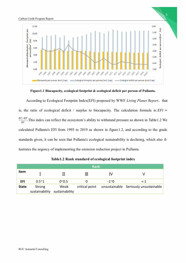
Analyzing the biocapacity(EC) and ecological footprint(EF) of Pullanta, we know the bio-
capacity per person fluctuates slightly and the overall trend is declining as shown in Table1.1 and
Figure1.1 The ecological footprint per person fluctuates more obviously and generally shows an
upward trend. What’s more important, an ecological deficit occur, that is, ecological footprint of
each year is greater than biocapacity. And the deficit is increasing, which means Pullanta is con-
suming natural resources faster than the ecosystem can recover, putting a lot of pressure on the
ecosystem and going against the concept of sustainable development. This means it’s urgent for
4 Carbon Credit Program Report
RUC Actuarial Consulting
Pullanta to take measures to reduce emission.
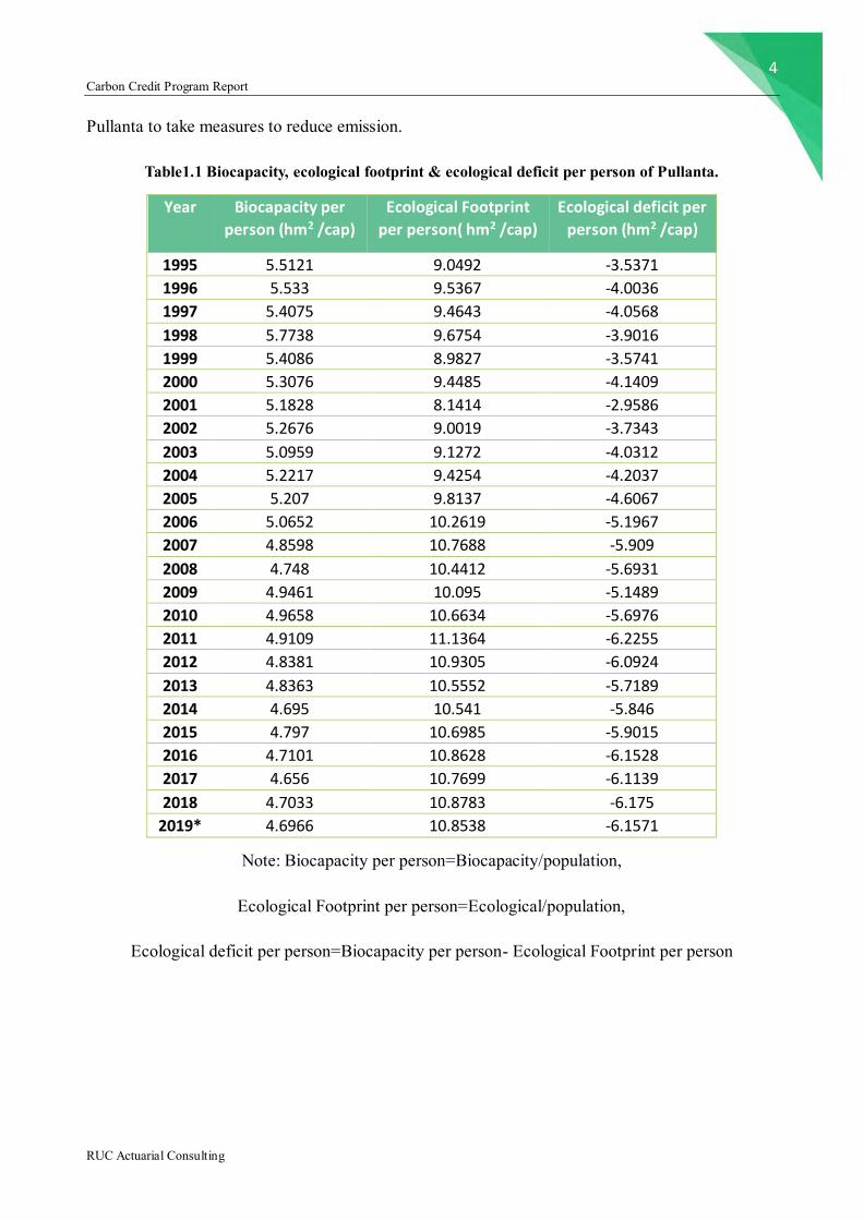
Table1.1 Biocapacity, ecological footprint & ecological deficit per person of Pullanta.
Year Biocapacity per
person (hm2 /cap)
Ecological Footprint
per person( hm2 /cap)
Ecological deficit per
person (hm2 /cap)
1995 5.5121 9.0492 -3.5371
1996 5.533 9.5367 -4.0036
1997 5.4075 9.4643 -4.0568
1998 5.7738 9.6754 -3.9016
1999 5.4086 8.9827 -3.5741
2000 5.3076 9.4485 -4.1409
2001 5.1828 8.1414 -2.9586
2002 5.2676 9.0019 -3.7343
2003 5.0959 9.1272 -4.0312
2004 5.2217 9.4254 -4.2037
2005 5.207 9.8137 -4.6067
2006 5.0652 10.2619 -5.1967
2007 4.8598 10.7688 -5.909
2008 4.748 10.4412 -5.6931
2009 4.9461 10.095 -5.1489
2010 4.9658 10.6634 -5.6976
2011 4.9109 11.1364 -6.2255
2012 4.8381 10.9305 -6.0924
2013 4.8363 10.5552 -5.7189
2014 4.695 10.541 -5.846
2015 4.797 10.6985 -5.9015
2016 4.7101 10.8628 -6.1528
2017 4.656 10.7699 -6.1139
2018 4.7033 10.8783 -6.175
2019* 4.6966 10.8538 -6.1571
Note: Biocapacity per person=Biocapacity/population,
Ecological Footprint per person=Ecological/population,
Ecological deficit per person=Biocapacity per person- Ecological Footprint per person
5 Carbon Credit Program Report
RUC Actuarial Consulting
Figure1.1 Biocapacity, ecological footprint & ecological deficit per person of Pullanta.
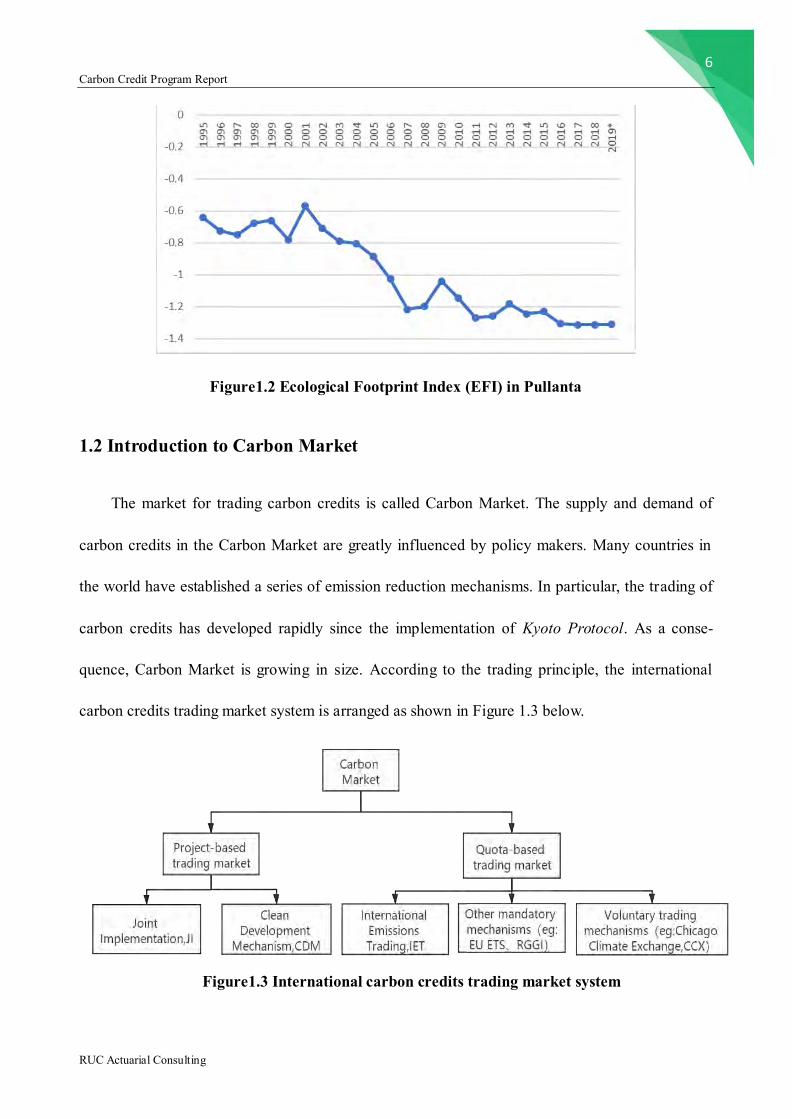
According to Ecological Footprint Index(EFI) proposed by WWF Living Planet Report,that
is, the ratio of ecological deficit / surplus to biocapacity. The calculation formula is:𝐸𝐹𝐼 =
𝐸𝐶−𝐸𝐹
𝐸𝐶.This index can reflect the ecosystem’s ability to withstand pressure as shown in Table1.2 We
calculated Pullanta's EFI from 1995 to 2019 as shown in figure1.2, and according to the grade
standards given, it can be seen that Pullanta's ecological sustainability is declining, which also il-
lustrates the urgency of implementing the emission reduction project in Pullanta.
Table1.2 Rank standard of ecological footprint index
Rank
Item Ⅰ Ⅱ Ⅲ Ⅳ Ⅴ
EFI 0.5~1 0~0.5 0 -1~0 <-1
State Strong
sustainability
Weak
sustainability
critical point unsustainable Seriously unsustainable
6 Carbon Credit Program Report
RUC Actuarial Consulting
Figure1.2 Ecological Footprint Index (EFI) in Pullanta
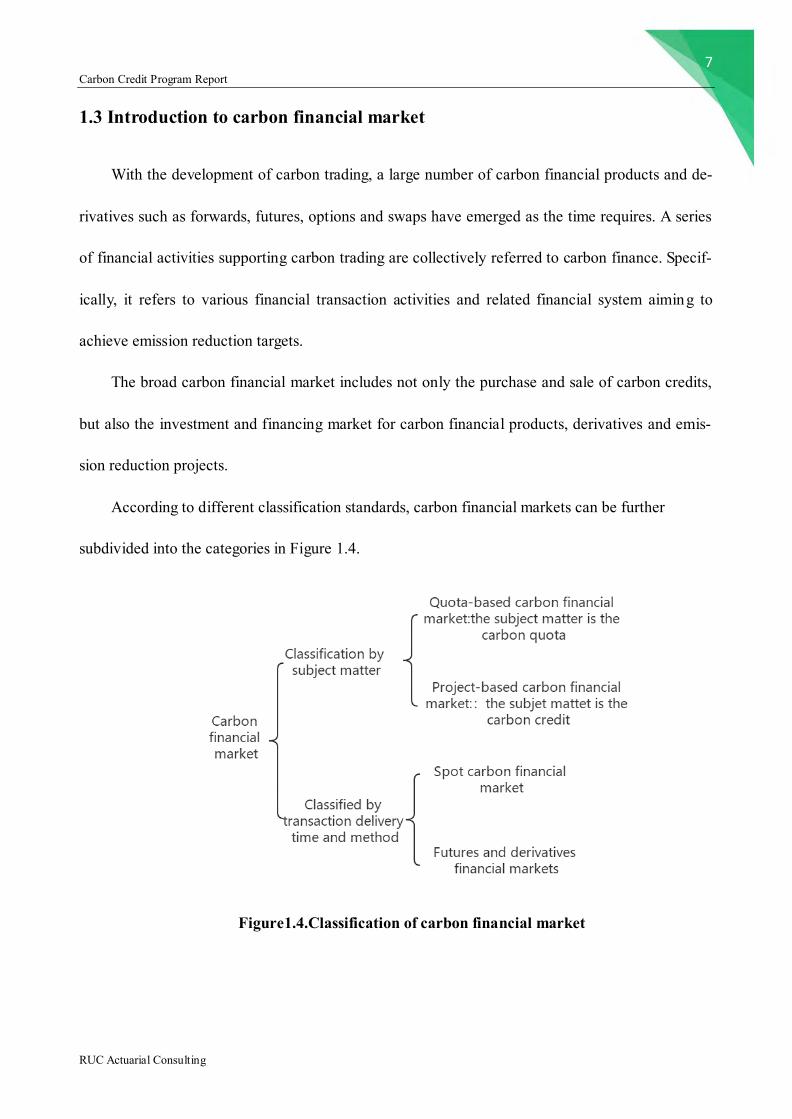
1.2 Introduction to Carbon Market
The market for trading carbon credits is called Carbon Market. The supply and demand of
carbon credits in the Carbon Market are greatly influenced by policy makers. Many countries in
the world have established a series of emission reduction mechanisms. In particular, the trading of
carbon credits has developed rapidly since the implementation of Kyoto Protocol. As a conse-
quence, Carbon Market is growing in size. According to the trading principle, the international
carbon credits trading market system is arranged as shown in Figure 1.3 below.
Figure1.3 International carbon credits trading market system
7 Carbon Credit Program Report
RUC Actuarial Consulting
1.3 Introduction to carbon financial market
With the development of carbon trading, a large number of carbon financial products and de-
rivatives such as forwards, futures, options and swaps have emerged as the time requires. A series
of financial activities supporting carbon trading are collectively referred to carbon finance. Specif-
ically, it refers to various financial transaction activities and related financial system aiming to
achieve emission reduction targets.
The broad carbon financial market includes not only the purchase and sale of carbon credits,
but also the investment and financing market for carbon financial products, derivatives and emis-
sion reduction projects.
According to different classification standards, carbon financial markets can be further
subdivided into the categories in Figure 1.4.
Figure1.4.Classification of carbon financial market

8 Carbon Credit Program Report
RUC Actuarial Consulting
1.4 Research Purpose
Our team will design a carbon credit plan for Pullanta to help it achieve emission reduction
targets and improve its ecological environment. At the same time, it will allow the government to
obtain revenue, and then invest in energy-saving and emission-reduction projects such as clean
energy and equipment renovation. With I view to alleviating the pressure on ecosystems and cli-
mate conditions.
We will also study the mechanism of carbon credit price formation, the price operation and
pricing mechanism of carbon spot, futures, and options. With a view to providing decision refer-
ence for the construction and development of Pullanta's carbon financial market.
In addition, we also hope that Pullanta’s plan can provide some experience for other countries
in the world.
9 Carbon Credit Program Report
RUC Actuarial Consulting
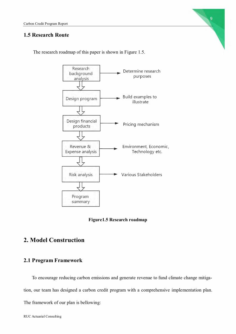
1.5 Research Route
The research roadmap of this paper is shown in Figure 1.5.
Figure1.5 Research roadmap
2. Model Construction
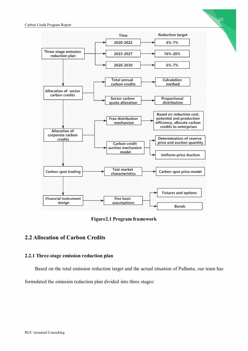
2.1 Program Framework
To encourage reducing carbon emissions and generate revenue to fund climate change mitiga-
tion, our team has designed a carbon credit program with a comprehensive implementation plan.
The framework of our plan is bellowing:
10 Carbon Credit Program Report
RUC Actuarial Consulting
Figure2.1 Program framework
2.2 Allocation of Carbon Credits
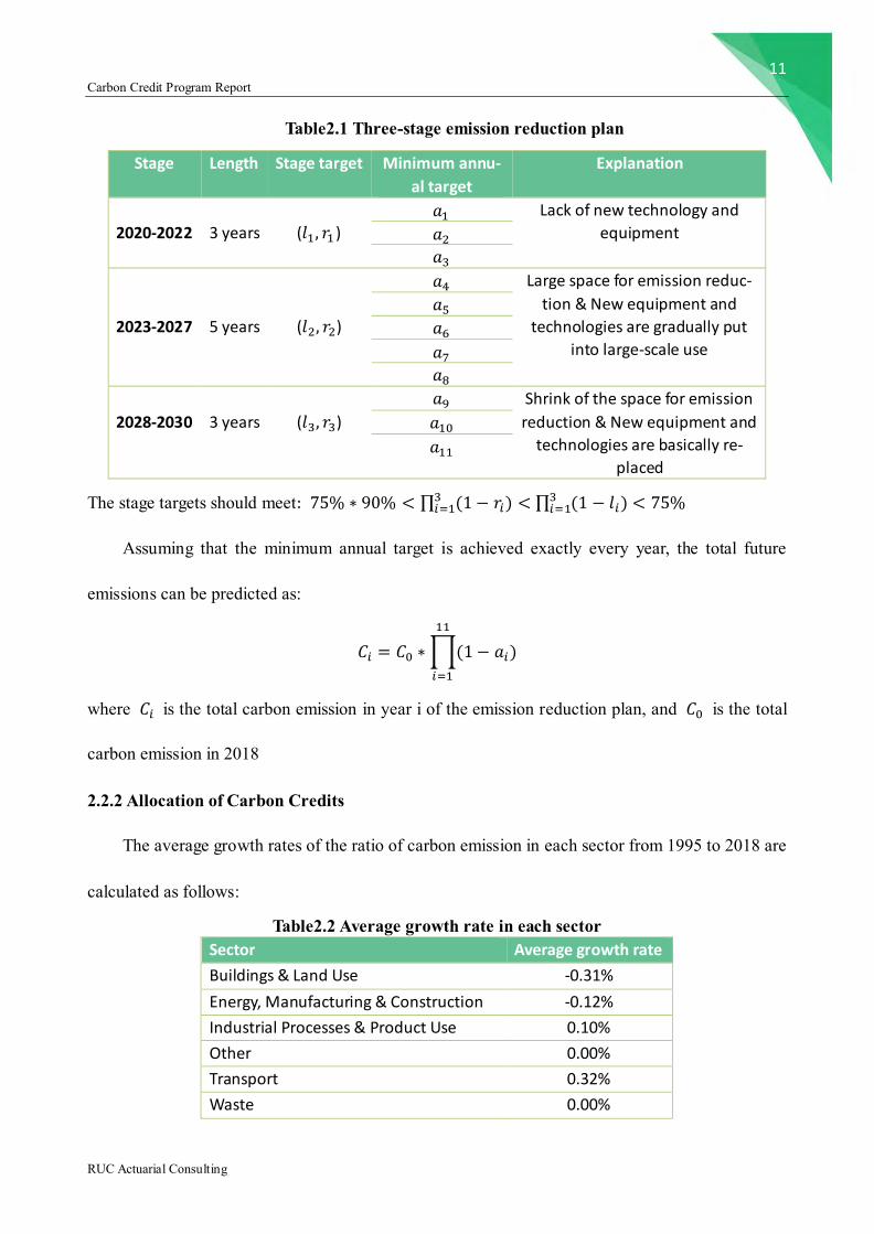
2.2.1 Three-stage emission reduction plan
Based on the total emission reduction target and the actual situation of Pullanta, our team has
formulated the emission reduction plan divided into three stages:
11 Carbon Credit Program Report
RUC Actuarial Consulting
Table2.1 Three-stage emission reduction plan
Stage Length Stage target Minimum annu-
al target
Explanation
2020-2022
3 years
(𝑙1, 𝑟1 )
𝑎1 Lack of new technology and
equipment 𝑎2
𝑎3
2023-2027
5 years
(𝑙2, 𝑟2)
𝑎4 Large space for emission reduc-
tion & New equipment and
technologies are gradually put
into large-scale use
𝑎5
𝑎6
𝑎7
𝑎8
2028-2030
3 years
(𝑙3, 𝑟3)
𝑎9 Shrink of the space for emission
reduction & New equipment and
technologies are basically re-
placed
𝑎10
𝑎11
The stage targets should meet: 75% ∗ 90% < ∏ (1− 𝑟𝑖)3𝑖=1 < ∏ (1 − 𝑙𝑖)
3𝑖=1 < 75%
Assuming that the minimum annual target is achieved exactly every year, the total future
emissions can be predicted as:
𝐶𝑖 = 𝐶0 ∗∏(1− 𝑎𝑖)
11
𝑖=1
where 𝐶𝑖 is the total carbon emission in year i of the emission reduction plan, and 𝐶0 is the total
carbon emission in 2018
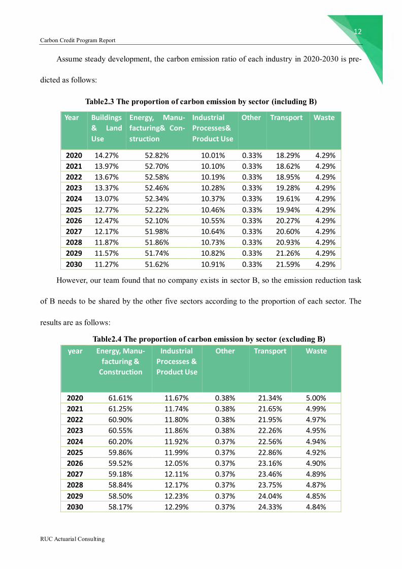
2.2.2 Allocation of Carbon Credits
The average growth rates of the ratio of carbon emission in each sector from 1995 to 2018 are
calculated as follows:
Table2.2 Average growth rate in each sector Sector Average growth rate
Buildings & Land Use -0.31%
Energy, Manufacturing & Construction -0.12%
Industrial Processes & Product Use 0.10%
Other 0.00%
Transport 0.32%
Waste 0.00%
12 Carbon Credit Program Report
RUC Actuarial Consulting
Assume steady development, the carbon emission ratio of each industry in 2020-2030 is pre-
dicted as follows:
Table2.3 The proportion of carbon emission by sector (including B)
Year Buildings
& Land
Use
Energy, Manu-
facturing& Con-
struction
Industrial
Processes&
Product Use
Other Transport Waste
2020 14.27% 52.82% 10.01% 0.33% 18.29% 4.29%
2021 13.97% 52.70% 10.10% 0.33% 18.62% 4.29%
2022 13.67% 52.58% 10.19% 0.33% 18.95% 4.29%
2023 13.37% 52.46% 10.28% 0.33% 19.28% 4.29%
2024 13.07% 52.34% 10.37% 0.33% 19.61% 4.29%
2025 12.77% 52.22% 10.46% 0.33% 19.94% 4.29%
2026 12.47% 52.10% 10.55% 0.33% 20.27% 4.29%
2027 12.17% 51.98% 10.64% 0.33% 20.60% 4.29%
2028 11.87% 51.86% 10.73% 0.33% 20.93% 4.29%
2029 11.57% 51.74% 10.82% 0.33% 21.26% 4.29%
2030 11.27% 51.62% 10.91% 0.33% 21.59% 4.29%
However, our team found that no company exists in sector B, so the emission reduction task
of B needs to be shared by the other five sectors according to the proportion of each sector. The
results are as follows:
Table2.4 The proportion of carbon emission by sector (excluding B) year Energy, Manu-
facturing &
Construction
Industrial
Processes &
Product Use
Other Transport Waste
2020 61.61% 11.67% 0.38% 21.34% 5.00%
2021 61.25% 11.74% 0.38% 21.65% 4.99%
2022 60.90% 11.80% 0.38% 21.95% 4.97%
2023 60.55% 11.86% 0.38% 22.26% 4.95%
2024 60.20% 11.92% 0.37% 22.56% 4.94%
2025 59.86% 11.99% 0.37% 22.86% 4.92%
2026 59.52% 12.05% 0.37% 23.16% 4.90%
2027 59.18% 12.11% 0.37% 23.46% 4.89%
2028 58.84% 12.17% 0.37% 23.75% 4.87%
2029 58.50% 12.23% 0.37% 24.04% 4.85%
2030 58.17% 12.29% 0.37% 24.33% 4.84%
13 Carbon Credit Program Report
RUC Actuarial Consulting
The carbon quota of each sector can be obtained by multiplying the proportion of each sector
by the total carbon emission each year. After obtaining the sector quota forecast, carbon quota is
allocated to enterprises in each sector according to their carbon emission ratio. Enterprises obtain
carbon credits through auction and free allocation from the government of Pullanta.
As for the proportion of free allocation and auction in each sector, different proportions can be
set at each stage or each year according to the actual situation of the emission reduction cost and
emission reduction potential of each sector.
2.2.3 Understanding of the emission reduction goal
Pullanta has a goal of reducing carbon emissions to 25% below the 2018 level by the end of
the year 2030 and needs a carbon credit program that is expected to result in total carbon emissions
staying within 90% of Pullanta’s goals with 90% certainty. From the perspective of probability
statistics, the probability of the total annual carbon emissions of 2030 is less than 75% of the total
annual carbon emissions of 2018 is 1, and the probability of the total annual carbon emissions of
2030 is less than 67.5% (=90%*75%) of the total annual carbon emissions of 2018 is 0.9.
In our program, the actual annual carbon emission reduction (the amount of actual annual
carbon emission reduction compared with 2018) is taken as the random variable X. 𝑋𝑡 represents
the actual emission reduction in year t. According to the overview, there is a lower limit for the
emission reduction, that is, the emission reduction must be greater than a certain value, in order to
be meaningful. The lower limit varies from year to year and is determined by the reduction target
for that year. Considering the characteristics of carbon emissions reduction, X, this article assumes
that X obeys the Single-parameter Pareto distribution.
The probability density function of the Single-parameter Pareto distribution is:
14 Carbon Credit Program Report
RUC Actuarial Consulting
𝑓(𝑥) =𝛼𝜃𝛼
𝑥𝛼+1, 𝑥 > 𝜃
And the cumulative distribution function is,
𝐹(𝑥) = 1 − (𝜃/𝑥)𝛼 , 𝑥 > 𝜃
In our program, we are interested in its tail distribution function, which is,
�̅�(𝑥) = Pr(𝑋 > 𝑥) = (𝜃/𝑥)𝛼 , 𝑥 > 𝜃
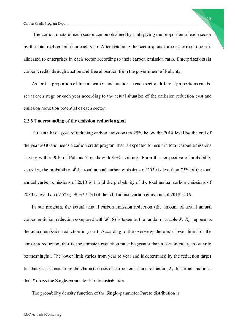
where, 𝜃 is the lower limit of carbon emissions reduction. Taking year of 2030 as an example,
the situation is as follows.
Figure2.2 Distribution of the actual carbon emissions in 2030
We can solve for 𝜃 = 230610266.1, 𝛼 = 0.4016.
Since the actual annual carbon emissions are also random variables, there must be a superior
limit of the total amount of carbon credits from government each year to ensure that the target can
be realized. In this model, the annual superior limit is equal to the difference between carbon
emissions in 2018 and the annual lower limit, 𝜃𝑡. The superior limit of the total amount of carbon
credits issued in the year t is 𝑌𝑡, because emission reduction will cause the increase of production

15 Carbon Credit Program Report
RUC Actuarial Consulting
costs of enterprises, which will lead to the increase of social costs, these increases will be passed
on to consumers. Considering the cost minimization, the total amount of carbon emission rights
issued by the government every year is 𝑌𝑡 .
2.3Auction model for carbon credit
Due to differences in emission reduction targets and freely allocated carbon credits in
different sectors, auctions will be conducted in different sectors. Pullanta can establish an online
auction system and require companies to submit bid prices and bid quantities within the prescribed
time once a quarter.
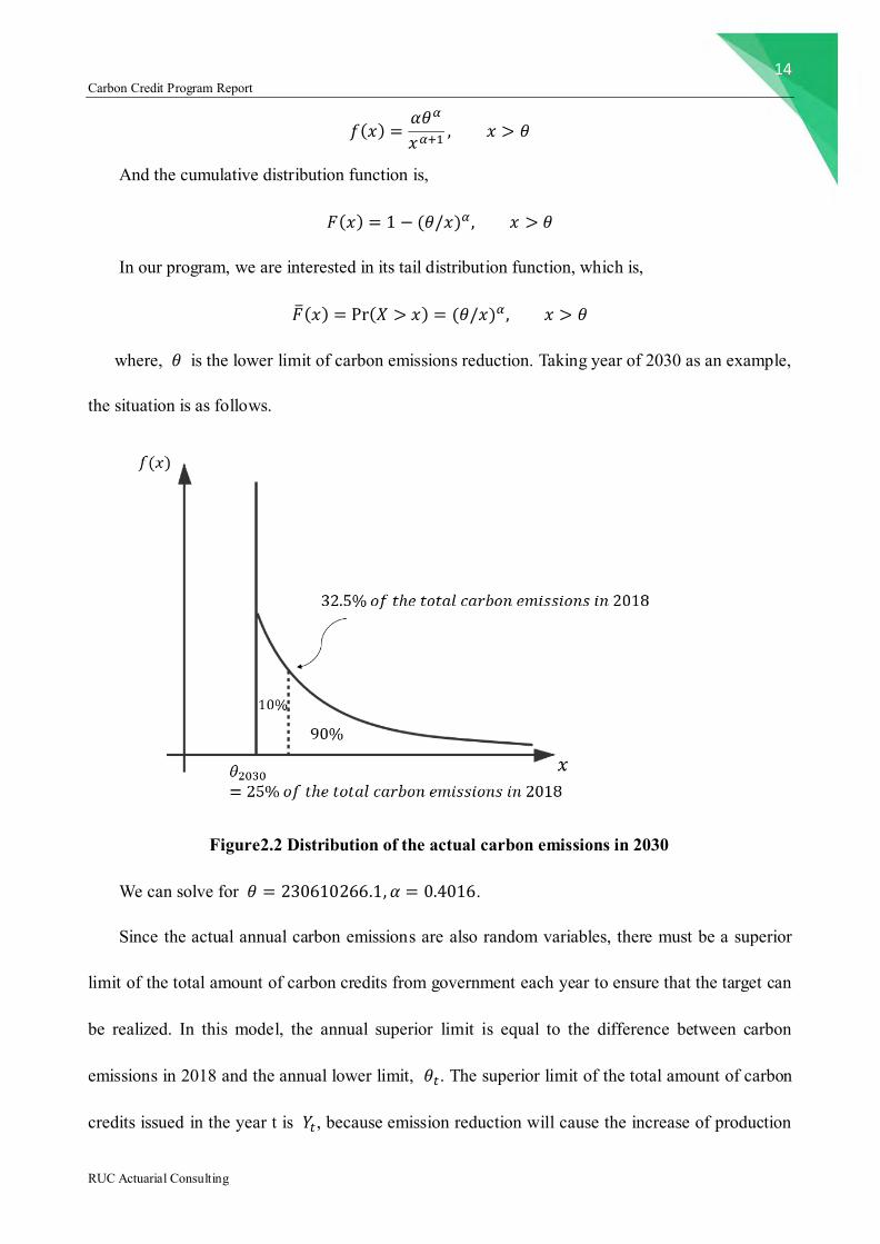
2.3.1 Liability of auction market agent
The relationship between auction market agents as shown below:
(1) Because the government is the seller and supervisor, it needs to:
①Determine the total carbon credits 𝑄𝑡 for each auction according to the overall emission
reduction targets of Pullanta;
②Determine the reserve price 𝑅𝑃𝑡 and maximum floating ratio 𝛼𝑡 for the 𝑡𝑡ℎ auction. We
can set the price based on revelent factors and pricing model which are mentioned in 2.4 as
original price 𝑂𝑅𝑃𝑡 . Then the government determines downscale 𝛽𝑡. Finally,
The reserve price 𝑅𝑃𝑡= original price 𝑂𝑅𝑃𝑡 × (1 − 𝛽𝑡).
The setting of these two ratios is mainly based on the actual situation in Pullanta. The
government should take the implementation effect of program, the feedback of enterprises, the
operational condition of carbon market, the emission pressure of enterprises and so on into
consideration. Besides, the government should refer to the setting of other international emission
16 Carbon Credit Program Report
RUC Actuarial Consulting
reduction programs.
(2) Companies are bidders.The model assumes that all companies make bidding strategies
based on profit-seeking purposes. And they make decisions independently, that is, they don’t
depend on other companies’ bidding information. In order to obtain the maximum economic
benefits, the bidder I needs to:
① adjust bidding strategies based on its own situation and previous external market
information;
②determines the bid price 𝑃𝑏𝑖,𝑡 and quantity 𝑞𝑖,𝑡 for the 𝑡𝑡ℎ auction.
Figure2.3 Relationship between carbon credit right auction market agents for any sector
17 Carbon Credit Program Report
RUC Actuarial Consulting
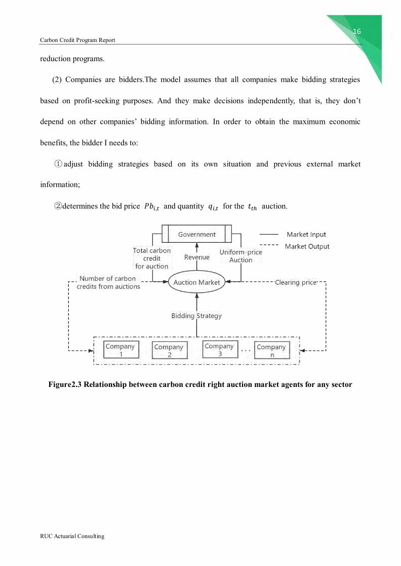
2.3.2 Auction market rules
Rules of the auction market as shown below:
Figure2.4 Process of auction of any time
There is a more detailed explanation about the purchase price 𝑃𝑖,𝑡 and market clearing price
𝐶𝑃𝑡 as follows. Note that purchase price 𝑃𝑖,𝑡 is the same as market clearing price 𝐶𝑃𝑡 because
the government adopts uniform-price auctions.
𝑃𝑖,𝑡 = 𝐶𝑃𝑡 =
{
𝑃𝑏𝑢+1,𝑡
∗ , 𝑖𝑓∑𝑞𝑖,𝑡∗ < 𝑄𝑡 ,
𝑢
𝑖=1
∑𝑞𝑖,𝑡∗ ≥ 𝑄𝑡
𝑢+1
𝑖=1
, 𝑖 ≤ 𝑢 + 1 (𝑎)
+∞, 𝑖𝑓∑𝑞𝑖,𝑡∗ < 𝑄𝑡 ,
𝑢
𝑖=1
∑𝑞𝑖,𝑡∗ ≥ 𝑄𝑡
𝑢+1
𝑖=1
, 𝑖 ≥ 𝑢 + 1 (𝑏)
𝑃𝑏𝑛,𝑡∗ , 𝑖𝑓∑𝑞𝑖,𝑡
∗ < 𝑄𝑡
𝑛
𝑖=1
(𝑐)
Figure 2.5 Clearing & purchase prices under different circumstances
18 Carbon Credit Program Report
RUC Actuarial Consulting
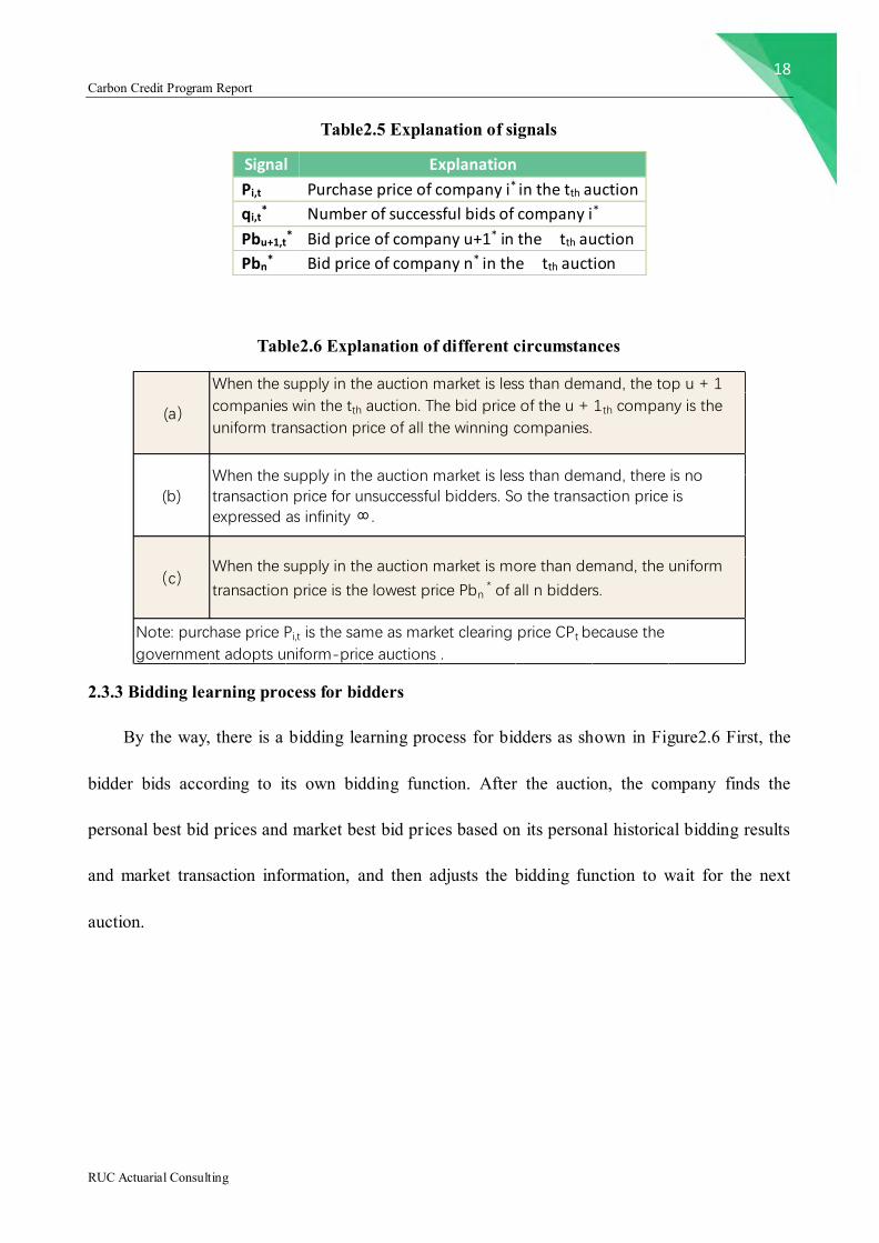
Table2.5 Explanation of signals
Signal Explanation
Pi,t Purchase price of company i* in the tth auction
qi,t* Number of successful bids of company i*
Pbu+1,t* Bid price of company u+1* in the tth auction
Pbn* Bid price of company n* in the tth auction
Table2.6 Explanation of different circumstances
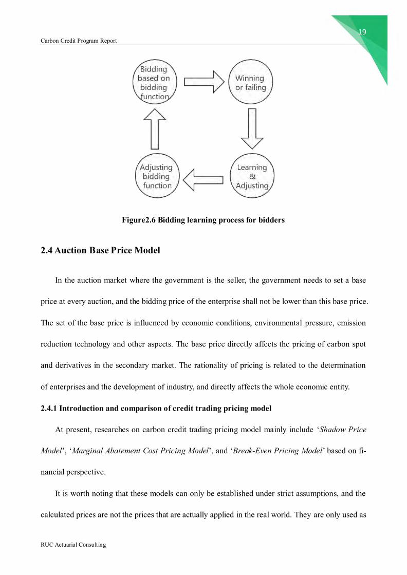
2.3.3 Bidding learning process for bidders
By the way, there is a bidding learning process for bidders as shown in Figure2.6 First, the
bidder bids according to its own bidding function. After the auction, the company finds the
personal best bid prices and market best bid prices based on its personal historical bidding results
and market transaction information, and then adjusts the bidding function to wait for the next
auction.
Note: purchase price Pi,t is the same as market clearing price CPt because the
government adopts uniform-price auctions .
(a)
When the supply in the auction market is less than demand, the top u + 1
companies win the tth auction. The bid price of the u + 1th company is the
uniform transaction price of all the winning companies.
(b)When the supply in the auction market is less than demand, there is notransaction price for unsuccessful bidders. So the transaction price isexpressed as infinity ∞.
(c)When the supply in the auction market is more than demand, the uniform
transaction price is the lowest price Pbn * of all n bidders.
19 Carbon Credit Program Report
RUC Actuarial Consulting
Figure2.6 Bidding learning process for bidders
2.4 Auction Base Price Model
In the auction market where the government is the seller, the government needs to set a base
price at every auction, and the bidding price of the enterprise shall not be lower than this base price.
The set of the base price is influenced by economic conditions, environmental pressure, emission
reduction technology and other aspects. The base price directly affects the pricing of carbon spot
and derivatives in the secondary market. The rationality of pricing is related to the determination
of enterprises and the development of industry, and directly affects the whole economic entity.
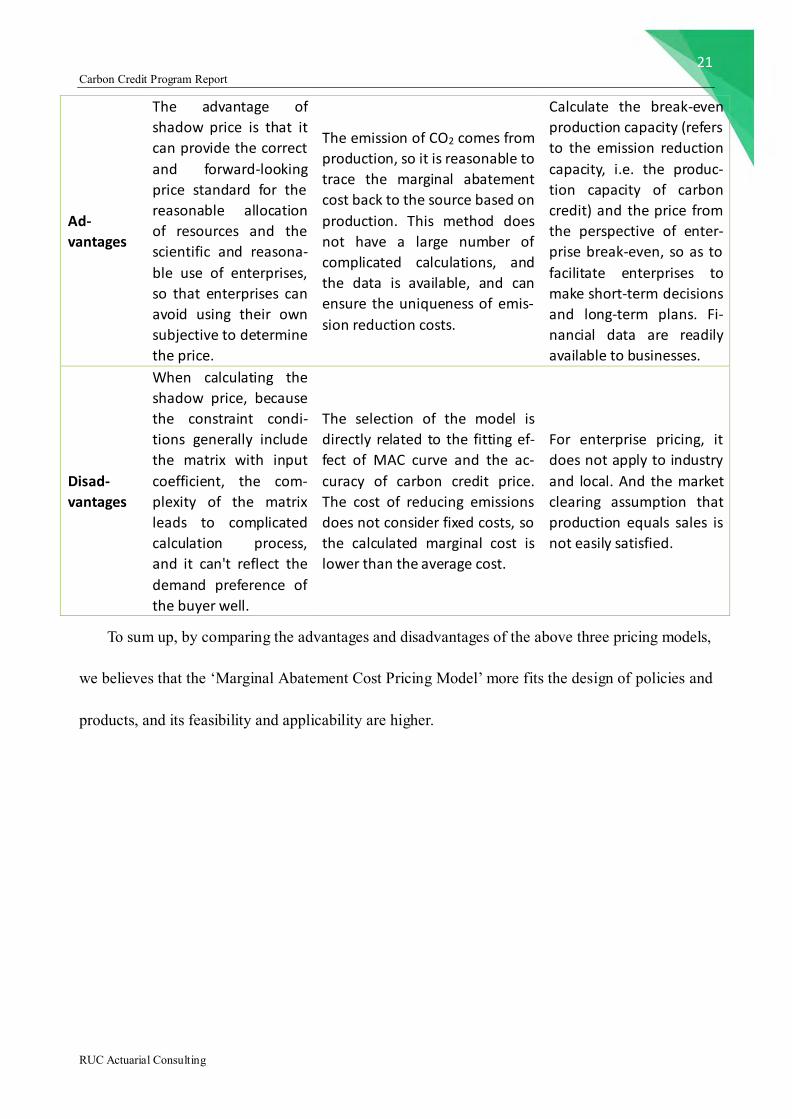
2.4.1 Introduction and comparison of credit trading pricing model
At present, researches on carbon credit trading pricing model mainly include ‘Shadow Price
Model’, ‘Marginal Abatement Cost Pricing Model’, and ‘Break-Even Pricing Model’ based on fi-
nancial perspective.
It is worth noting that these models can only be established under strict assumptions, and the
calculated prices are not the prices that are actually applied in the real world. They are only used as
20 Carbon Credit Program Report
RUC Actuarial Consulting
a reference for pricing, and the actual pricing needs to consider about various uncertain factors.
The following table compares these three kinds of models.
Table2.7 Three kinds of carbon credit pricing models
Pricing
Methods Shadow Price Model
Marginal Abatement Cost Pric-
ing Model Break-Even Pricing Model
Details
Shadow price, also
known as optimal plan
price or optimal calcu-
lated price. The United
Nations believes that
shadow prices is a kind
of opportunity cost for
enterprises from put-
ting financial resources,
material resources and
human resources into
their production.
Shadow prices actually
measure the marginal
benefit, or marginal
contribution, of an ex-
tra unit of resources,
reflecting the scarcity
and true value of re-
sources.
Marginal Abatement Cost (MAC)
refers to the economic cost of
reducing one unit of CO2 emis-
sion at a certain emission level.
With the increase of emission
reduction, the difficulty of emis-
sion reduction gradually in-
creases, and the marginal
abatement cost increases (de-
creases first and then increases
later).
Marginal abatement cost is a
pricing method based on mar-
ginal cost theory. Enterprises
whose marginal abatement cost
is lower than the market price of
carbon credit will choose to re-
duce emissions as much as pos-
sible, while other enterprises
will choose to buy carbon credit
to meet the emission standards.
All enterprises will optimize
their behaviors for the maxi-
mum profit and ultimately
achieve ‘Pareto Optimization’.
Break-Even pricing meth-
ods, refers to when the
sales is certain, the price
of products must reach a
certain level to achieve
break-even. The key of
break-even analysis is to
determine the break-even
point, which is the state
when profit is zero.
Assump-
tion
Perfectly competitive
market
Sales volume is the only
cost driver of market
clearing
Calculate
Methods
Dual solutions for linear
programming;
Lagrange multiplier
method
By deducing the marginal
abatement cost curve of a cer-
tain place or a certain industry
through the model, and then
the marginal abatement cost of
CO2, namely carbon credit price,
can be further eliminated by
maximizing corporate profits.
Cost-Volume-Profit Analy-
sis, CVP, the price of the
equilibrium point is the
price when the company's
sales revenue is equal to
total cost (fixed cost +
variable cost)
21 Carbon Credit Program Report
RUC Actuarial Consulting
Ad-
vantages
The advantage of
shadow price is that it
can provide the correct
and forward-looking
price standard for the
reasonable allocation
of resources and the
scientific and reasona-
ble use of enterprises,
so that enterprises can
avoid using their own
subjective to determine
the price.
The emission of CO2 comes from
production, so it is reasonable to
trace the marginal abatement
cost back to the source based on
production. This method does
not have a large number of
complicated calculations, and
the data is available, and can
ensure the uniqueness of emis-
sion reduction costs.
Calculate the break-even
production capacity (refers
to the emission reduction
capacity, i.e. the produc-
tion capacity of carbon
credit) and the price from
the perspective of enter-
prise break-even, so as to
facilitate enterprises to
make short-term decisions
and long-term plans. Fi-
nancial data are readily
available to businesses.
Disad-
vantages
When calculating the
shadow price, because
the constraint condi-
tions generally include
the matrix with input
coefficient, the com-
plexity of the matrix
leads to complicated
calculation process,
and it can't reflect the
demand preference of
the buyer well.
The selection of the model is
directly related to the fitting ef-
fect of MAC curve and the ac-
curacy of carbon credit price.
The cost of reducing emissions
does not consider fixed costs, so
the calculated marginal cost is
lower than the average cost.
For enterprise pricing, it
does not apply to industry
and local. And the market
clearing assumption that
production equals sales is
not easily satisfied.
To sum up, by comparing the advantages and disadvantages of the above three pricing models,
we believes that the ‘Marginal Abatement Cost Pricing Model’ more fits the design of policies and
products, and its feasibility and applicability are higher.
22 Carbon Credit Program Report
RUC Actuarial Consulting
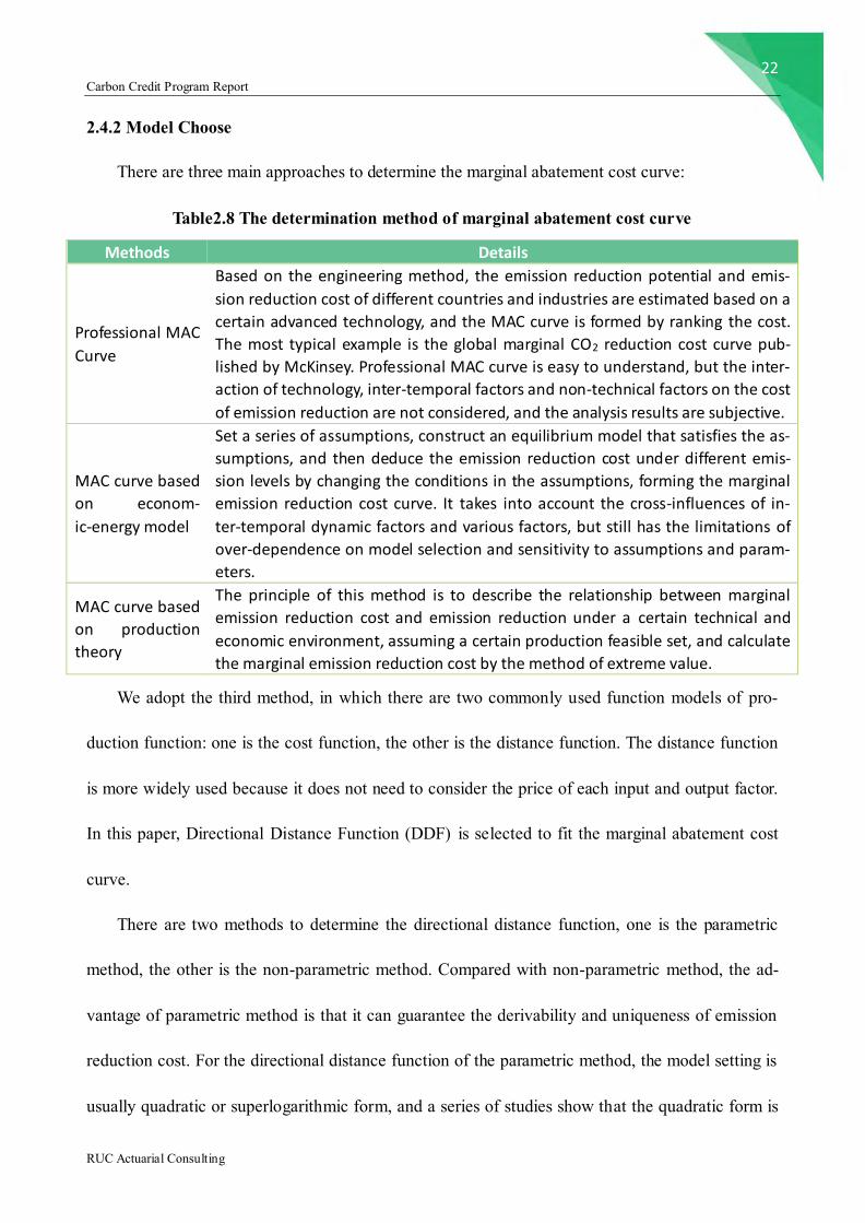
2.4.2 Model Choose
There are three main approaches to determine the marginal abatement cost curve:
Table2.8 The determination method of marginal abatement cost curve
Methods Details
Professional MAC
Curve
Based on the engineering method, the emission reduction potential and emis-
sion reduction cost of different countries and industries are estimated based on a
certain advanced technology, and the MAC curve is formed by ranking the cost.
The most typical example is the global marginal CO2 reduction cost curve pub-
lished by McKinsey. Professional MAC curve is easy to understand, but the inter-
action of technology, inter-temporal factors and non-technical factors on the cost
of emission reduction are not considered, and the analysis results are subjective.
MAC curve based
on econom-
ic-energy model
Set a series of assumptions, construct an equilibrium model that satisfies the as-
sumptions, and then deduce the emission reduction cost under different emis-
sion levels by changing the conditions in the assumptions, forming the marginal
emission reduction cost curve. It takes into account the cross-influences of in-
ter-temporal dynamic factors and various factors, but still has the limitations of
over-dependence on model selection and sensitivity to assumptions and param-
eters.
MAC curve based
on production
theory
The principle of this method is to describe the relationship between marginal
emission reduction cost and emission reduction under a certain technical and
economic environment, assuming a certain production feasible set, and calculate
the marginal emission reduction cost by the method of extreme value.
We adopt the third method, in which there are two commonly used function models of pro-
duction function: one is the cost function, the other is the distance function. The distance function
is more widely used because it does not need to consider the price of each input and output factor.
In this paper, Directional Distance Function (DDF) is selected to fit the marginal abatement cost
curve.
There are two methods to determine the directional distance function, one is the parametric
method, the other is the non-parametric method. Compared with non-parametric method, the ad-
vantage of parametric method is that it can guarantee the derivability and uniqueness of emission
reduction cost. For the directional distance function of the parametric method, the model setting is
usually quadratic or superlogarithmic form, and a series of studies show that the quadratic form is
23 Carbon Credit Program Report
RUC Actuarial Consulting
better than the superlogarithmic form. Therefore, we choose the quadratic directional distance
function to estimate the marginal abatement cost of CO2, so as to provide the reference price of
carbon credit in the auction market.
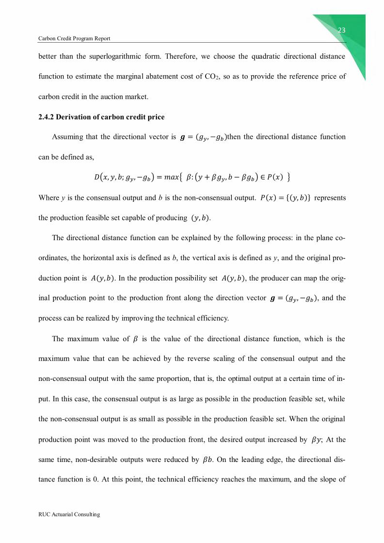
2.4.2 Derivation of carbon credit price
Assuming that the directional vector is 𝒈 = (𝑔𝑦, −𝑔𝑏)then the directional distance function
can be defined as,
𝐷(𝑥, 𝑦, 𝑏; 𝑔𝑦, −𝑔𝑏) = 𝑚𝑎𝑥{ 𝛽: (𝑦 + 𝛽𝑔𝑦, 𝑏 − 𝛽𝑔𝑏) ∈ 𝑃(𝑥) }
Where y is the consensual output and b is the non-consensual output. 𝑃(𝑥) = {(𝑦, 𝑏)} represents
the production feasible set capable of producing (𝑦, 𝑏).
The directional distance function can be explained by the following process: in the plane co-
ordinates, the horizontal axis is defined as b, the vertical axis is defined as y, and the original pro-
duction point is 𝐴(𝑦,𝑏). In the production possibility set 𝐴(𝑦, 𝑏), the producer can map the orig-
inal production point to the production front along the direction vector 𝒈 = (𝑔𝑦, −𝑔𝑏), and the
process can be realized by improving the technical efficiency.
The maximum value of 𝛽 is the value of the directional distance function, which is the
maximum value that can be achieved by the reverse scaling of the consensual output and the
non-consensual output with the same proportion, that is, the optimal output at a certain time of in-
put. In this case, the consensual output is as large as possible in the production feasible set, while
the non-consensual output is as small as possible in the production feasible set. When the original
production point was moved to the production front, the desired output increased by 𝛽𝑦; At the
same time, non-desirable outputs were reduced by 𝛽𝑏. On the leading edge, the directional dis-
tance function is 0. At this point, the technical efficiency reaches the maximum, and the slope of
24 Carbon Credit Program Report
RUC Actuarial Consulting
the tangent line on the direction front is − 𝑞
𝑝, where 𝑞 is the price of the non-desirable output, and
𝑝 is the price of the desirable output.
Let 𝑅 represent the maximum return that the producer can get, that is, the return
𝑅(𝑥, 𝑝, 𝑞) = 𝑚𝑎𝑥{ 𝑝𝑦 − 𝑞𝑏:𝐷(𝑥, 𝑦, 𝑏; 𝑔𝑦, −𝑔𝑏) ≥ 0 }
When 𝒈 = (𝑔𝑦, −𝑔𝑏) = (1, −1), the expression for the return can be expressed as,
𝑅(𝑥, 𝑝, 𝑞) = max𝑦,𝑏
{ 𝑝𝑦 − 𝑞𝑏:𝐷(𝑥, 𝑦, 𝑏; 1, −1) ≥ 0 }
Construct the Lagrangian function and take the derivative,
{
(𝑝 × 1 + 𝑞 × 1) ×𝜕𝐷(𝑥,𝑦, 𝑏; 1, −1)
𝜕𝑦= −𝑝
(𝑝 × 1 + 𝑞 × 1) ×𝜕𝐷(𝑥,𝑦, 𝑏; 1, −1)
𝜕𝑏= 𝑞
If we take the ratio of the two equations, we can get the price of undesirable output as fol-
lows,
𝑞 = −𝑝 ×𝜕𝐷/𝜕𝑏
𝜕𝐷/𝜕𝑦
In our program, desirable output 𝑦 is the GDP, output 𝑏 represents CO2 emissions, GDP is
priced by Pulo (Ƥ), the price of 𝑝 can be normalized to 1, then the price of CO2 marginal cost is,
𝑞 = −𝜕𝐷/𝜕𝑏
𝜕𝐷/𝜕𝑦
The specific form of quadratic directional distance function is as follows,
𝐷(𝑥, 𝑦,𝑏; 1,−1) = 𝛼0 + ∑ 𝛼𝑛𝑥𝑛3𝑛=1 + 𝛽1𝑦 + 𝛾1𝑏 +
1
2∑ ∑ 𝛼𝑛𝑚𝑥𝑛𝑥𝑚
3𝑚=1
3𝑛=1 +
1
2𝛽2𝑦
2 +1
2𝛾2𝑏
2 +
∑ 𝛿𝑛𝑥𝑛𝑦3𝑛=1 +∑ 𝜎𝑛𝑥𝑛𝑏
3𝑛=1 + 𝜇𝑦𝑏
Thus, the expression of marginal emission reduction cost is derived as,
𝑞 = −
𝜕𝐷𝜕𝑏𝜕𝐷𝜕𝑦
= −𝛾1 + 𝛾2𝑏 + ∑ 𝜎𝑛𝑥𝑛
3𝑛=1 + 𝜇𝑦
𝛽1 + 𝛽2𝑦 + ∑ 𝛿𝑛𝑥𝑛3𝑛=1 + 𝜇𝑏
25 Carbon Credit Program Report
RUC Actuarial Consulting
3. Case interpretation
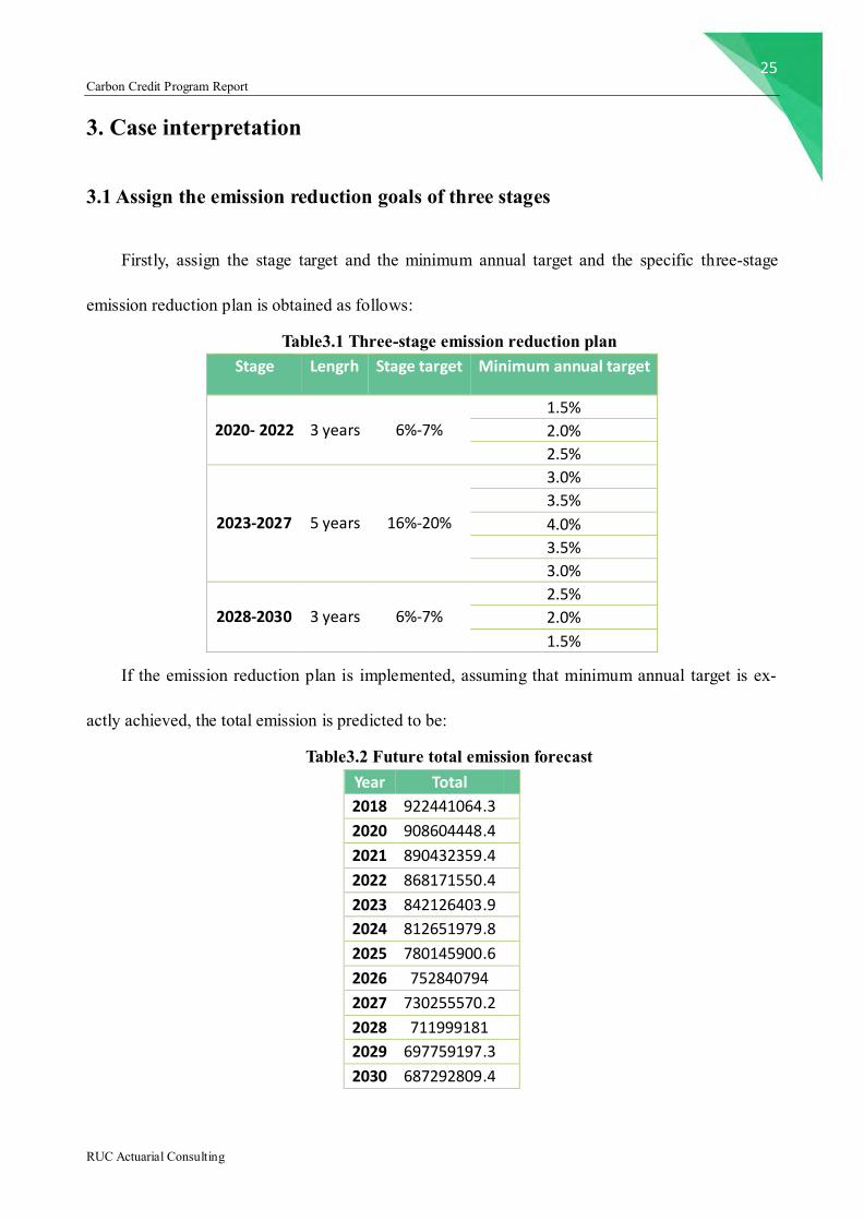
3.1 Assign the emission reduction goals of three stages
Firstly, assign the stage target and the minimum annual target and the specific three-stage
emission reduction plan is obtained as follows:
Table3.1 Three-stage emission reduction plan Stage Lengrh Stage target Minimum annual target
2020- 2022
3 years
6%-7%
1.5%
2.0%
2.5%
2023-2027
5 years
16%-20%
3.0%
3.5%
4.0%
3.5%
3.0%
2028-2030
3 years
6%-7%
2.5%
2.0%
1.5%
If the emission reduction plan is implemented, assuming that minimum annual target is ex-
actly achieved, the total emission is predicted to be:
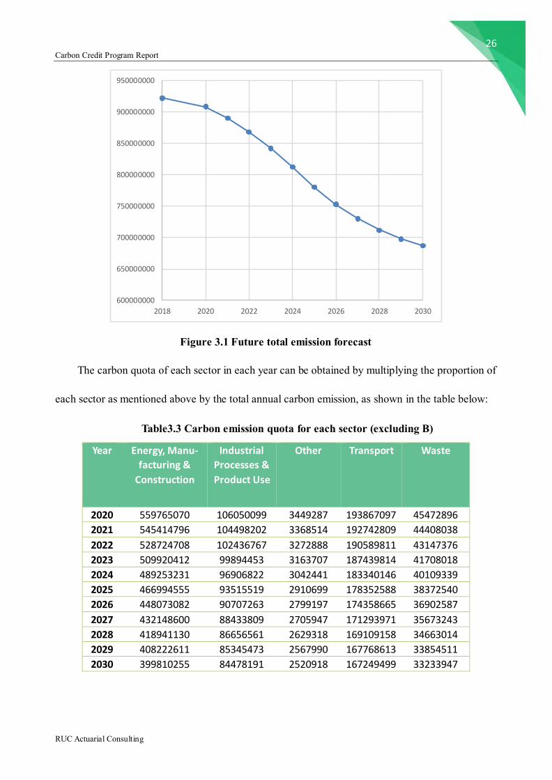
Table3.2 Future total emission forecast Year Total 2018 922441064.3 2020 908604448.4 2021 890432359.4 2022 868171550.4 2023 842126403.9 2024 812651979.8 2025 780145900.6 2026 752840794 2027 730255570.2 2028 711999181 2029 697759197.3 2030 687292809.4
26 Carbon Credit Program Report
RUC Actuarial Consulting
Figure 3.1 Future total emission forecast
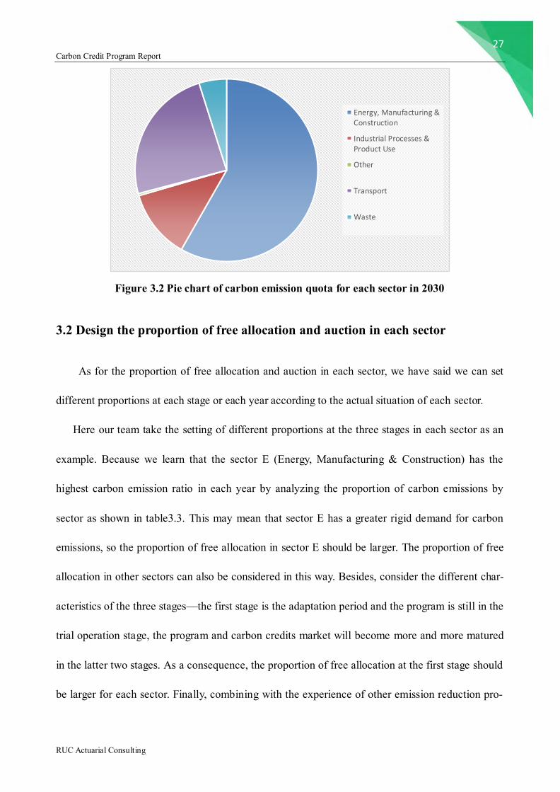
The carbon quota of each sector in each year can be obtained by multiplying the proportion of
each sector as mentioned above by the total annual carbon emission, as shown in the table below:
Table3.3 Carbon emission quota for each sector (excluding B)
Year Energy, Manu-
facturing &
Construction
Industrial
Processes &
Product Use
Other Transport Waste
2020 559765070 106050099 3449287 193867097 45472896
2021 545414796 104498202 3368514 192742809 44408038
2022 528724708 102436767 3272888 190589811 43147376
2023 509920412 99894453 3163707 187439814 41708018
2024 489253231 96906822 3042441 183340146 40109339
2025 466994555 93515519 2910699 178352588 38372540
2026 448073082 90707263 2799197 174358665 36902587
2027 432148600 88433809 2705947 171293971 35673243
2028 418941130 86656561 2629318 169109158 34663014
2029 408222611 85345473 2567990 167768613 33854511
2030 399810255 84478191 2520918 167249499 33233947
600000000
650000000
700000000
750000000
800000000
850000000
900000000
950000000
2018 2020 2022 2024 2026 2028 2030
27 Carbon Credit Program Report
RUC Actuarial Consulting
Figure 3.2 Pie chart of carbon emission quota for each sector in 2030
3.2 Design the proportion of free allocation and auction in each sector
As for the proportion of free allocation and auction in each sector, we have said we can set
different proportions at each stage or each year according to the actual situation of each sector.
Here our team take the setting of different proportions at the three stages in each sector as an
example. Because we learn that the sector E (Energy, Manufacturing & Construction) has the
highest carbon emission ratio in each year by analyzing the proportion of carbon emissions by
sector as shown in table3.3. This may mean that sector E has a greater rigid demand for carbon
emissions, so the proportion of free allocation in sector E should be larger. The proportion of free
allocation in other sectors can also be considered in this way. Besides, consider the different char-
acteristics of the three stages—the first stage is the adaptation period and the program is still in the
trial operation stage, the program and carbon credits market will become more and more matured
in the latter two stages. As a consequence, the proportion of free allocation at the first stage should
be larger for each sector. Finally, combining with the experience of other emission reduction pro-
Energy, Manufacturing &Construction
Industrial Processes &Product Use
Other
Transport
Waste
28 Carbon Credit Program Report
RUC Actuarial Consulting
grams in the world, we list the table of auction proportions of each sector at three stages as an ex-
ample.
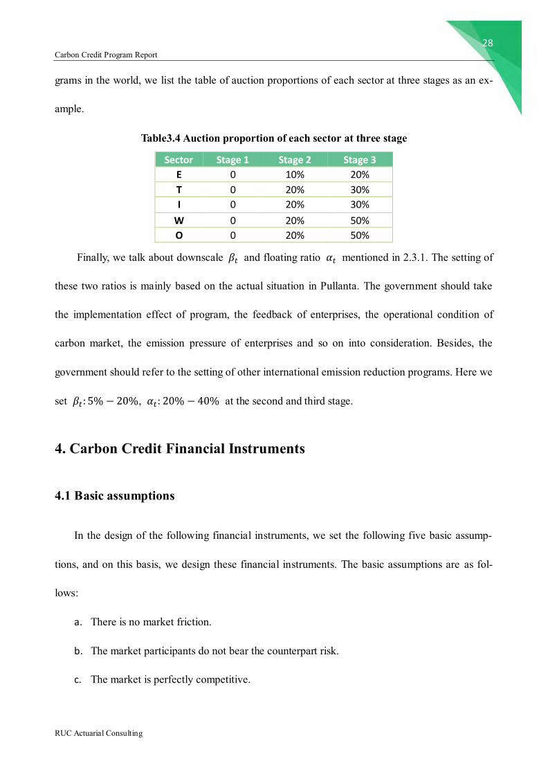
Table3.4 Auction proportion of each sector at three stage
Sector Stage 1 Stage 2 Stage 3
E 0 10% 20%
T 0 20% 30%
I 0 20% 30%
W 0 20% 50%
O 0 20% 50%
Finally, we talk about downscale 𝛽𝑡 and floating ratio 𝛼𝑡 mentioned in 2.3.1. The setting of
these two ratios is mainly based on the actual situation in Pullanta. The government should take
the implementation effect of program, the feedback of enterprises, the operational condition of
carbon market, the emission pressure of enterprises and so on into consideration. Besides, the
government should refer to the setting of other international emission reduction programs. Here we
set 𝛽𝑡: 5% − 20%, 𝛼𝑡: 20% − 40% at the second and third stage.
4. Carbon Credit Financial Instruments
4.1 Basic assumptions
In the design of the following financial instruments, we set the following five basic assump-
tions, and on this basis, we design these financial instruments. The basic assumptions are as fol-
lows:
a. There is no market friction.
b. The market participants do not bear the counterpart risk.
c. The market is perfectly competitive.
29 Carbon Credit Program Report
RUC Actuarial Consulting
d. Market participants are risk averse and want as much wealth as possible.
e. There is no arbitrage opportunity in the market.
4.2 Carbon spot price model
Analyzing existing empirical results, we know that the carbon trading market has fractal and
jump characteristics. Therefore, the jump fractional Brownian process may be a more suitable sto-
chastic process for modeling carbon trading prices. The jump fractal process is further applied to
the valuation of carbon financial products.
4.2.1 Testing of market characteristics
Due to the limited availability of data and considering that EU ETS is more mature, we use
the BlueNext Exchange CER cash and futures trading data from 2011 to 2013 as research objects.
And we mainly carry out empirical test of the fractal and jump characteristics of carbon trading
market.
4.2.1.1Testing of fractal characteristic
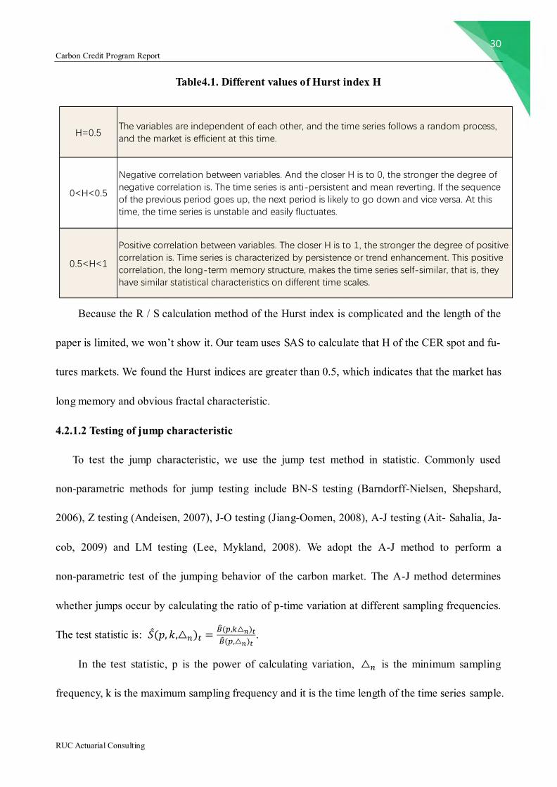
To test the fractal characteristic, we use R/S method proposed by Hurst (1951). Hurst discov-
ered the relation in 1951: log(𝑅𝑆) = 𝐻𝑙𝑜𝑔𝑛 + 𝑙𝑜𝑔𝑐, where R / S is the recalibration domain, c is a
constant, n is the number of observations, H is the Hurst index. Different values of Hurst index can
reveal different problems, as shown in Table4.1
30 Carbon Credit Program Report
RUC Actuarial Consulting
Table4.1. Different values of Hurst index H
Because the R / S calculation method of the Hurst index is complicated and the length of the
paper is limited, we won’t show it. Our team uses SAS to calculate that H of the CER spot and fu-
tures markets. We found the Hurst indices are greater than 0.5, which indicates that the market has
long memory and obvious fractal characteristic.
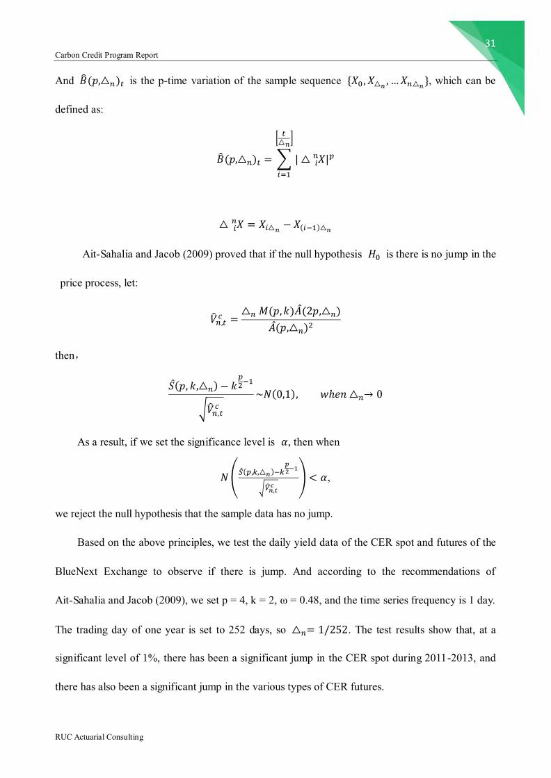
4.2.1.2 Testing of jump characteristic
To test the jump characteristic, we use the jump test method in statistic. Commonly used
non-parametric methods for jump testing include BN-S testing (Barndorff-Nielsen, Shepshard,
2006), Z testing (Andeisen, 2007), J-O testing (Jiang-Oomen, 2008), A-J testing (Ait- Sahalia, Ja-
cob, 2009) and LM testing (Lee, Mykland, 2008). We adopt the A-J method to perform a
non-parametric test of the jumping behavior of the carbon market. The A-J method determines
whether jumps occur by calculating the ratio of p-time variation at different sampling frequencies.
The test statistic is: 𝑆(𝑝, 𝑘,△𝑛)𝑡 =�̂�(𝑝,𝑘△𝑛)𝑡
�̂�(𝑝,△𝑛)𝑡.
In the test statistic, p is the power of calculating variation, △𝑛 is the minimum sampling
frequency, k is the maximum sampling frequency and it is the time length of the time series sample.
H=0.5
0<H<0.5
0.5<H<1
Positive correlation between variables. The closer H is to 1, the stronger the degree of positivecorrelation is. Time series is characterized by persistence or trend enhancement. This positivecorrelation, the long-term memory structure, makes the time series self-similar, that is, theyhave similar statistical characteristics on different time scales.
The variables are independent of each other, and the time series follows a random process,and the market is efficient at this time.
Negative correlation between variables. And the closer H is to 0, the stronger the degree ofnegative correlation is. The time series is anti-persistent and mean reverting. If the sequenceof the previous period goes up, the next period is likely to go down and vice versa. At thistime, the time series is unstable and easily fluctuates.
31 Carbon Credit Program Report
RUC Actuarial Consulting
And �̂�(𝑝,△𝑛)𝑡 is the p-time variation of the sample sequence {𝑋0 , 𝑋△𝑛 , …𝑋𝑛△𝑛}, which can be
defined as:
�̂�(𝑝,△𝑛)𝑡 = ∑ |△ 𝑋𝑖𝑛 |𝑝
[𝑡△𝑛
]
𝑖=1
△ 𝑋𝑖𝑛 = 𝑋𝑖△𝑛
− 𝑋(𝑖−1)△𝑛
Ait-Sahalia and Jacob (2009) proved that if the null hypothesis 𝐻0 is there is no jump in the
price process, let:
�̂�𝑛,𝑡𝑐 =
△𝑛 𝑀(𝑝,𝑘)�̂�(2𝑝,△𝑛)
�̂�(𝑝,△𝑛)2
then,
𝑆(𝑝, 𝑘,△𝑛) − 𝑘𝑝2−1
√�̂�𝑛,𝑡𝑐
~𝑁(0,1), 𝑤ℎ𝑒𝑛 △𝑛→ 0
As a result, if we set the significance level is 𝛼, then when
𝑁(�̂�(𝑝,𝑘,△𝑛)−𝑘
𝑝2−1
√𝑉𝑛,𝑡𝑐
) < 𝛼,
we reject the null hypothesis that the sample data has no jump.
Based on the above principles, we test the daily yield data of the CER spot and futures of the
BlueNext Exchange to observe if there is jump. And according to the recommendations of
Ait-Sahalia and Jacob (2009), we set p = 4, k = 2, ω = 0.48, and the time series frequency is 1 day.
The trading day of one year is set to 252 days, so △𝑛= 1/252. The test results show that, at a
significant level of 1%, there has been a significant jump in the CER spot during 2011-2013, and
there has also been a significant jump in the various types of CER futures.

32 Carbon Credit Program Report
RUC Actuarial Consulting
So far, we have verified that it is appropriate to model carbon prices by using the jump frac-
tional Brownian process.
4.2.2 Modeling carbon spot price
In order to represent the model conveniently, we firstly give the symbols used in this section
in the table below.
Table 4.2 Explanation of signals
Signal Meaning Signal Meaning
St Carbon spot price at
time t
{BtH} Fractional Brownian motion with Hurst
index H
{Nt} Poisson process with
intensity λ
{Yt} The jump amplitude following the
lognormal distribution, ln(Yt)~N(μy,σy)
X Option strike price rf Pulo's risk-free interest rate, set to con-
stant
σB Yield volatility of un-
derlying asset
rq Euro's risk-free interest rate, set to con-
stant
Δt Time interval of time
series data: Year
T Option expiration date
Suppose that the carbon spot price obeys the geometric fractal Brownian motion. The price
process under risk neutrality is:
𝑑𝑆𝑡 = 𝑟𝑞𝑆𝑡𝑑𝑡 + 𝜎𝑆𝑡𝑑𝐵𝑡𝐻, 𝑡 ≥ 0
From the Ito formula under Wick-Ito-Skorohod integral, we can get:
𝑑𝑙𝑛𝑆𝑡 = 𝑟𝑞𝑑𝑡 + 𝜎𝑑𝐵𝑡𝐻 − 𝜎2𝐻𝑡2𝐻−1𝑑𝑡
so
𝑣𝑎𝑟(△ 𝑙𝑛𝑆(𝑡)) = 𝜎2𝐻(△ 𝑡)2
As for the price volatility of carbon spot, it can be estimated by using historical carbon price data.
The estimation formula is:
33 Carbon Credit Program Report
RUC Actuarial Consulting
𝜎2 =1
(△ 𝑡)2𝐻∗
1
𝑛 − 1∑(𝑟𝑡𝑖 − �̅�
𝑛
𝑖=1
)2
where,𝑟𝑡𝑖 = 𝑙𝑛𝑆𝑡𝑖 − 𝑙𝑛𝑠𝑡𝑖−1, �̅� =1
𝑛∑ 𝑟𝑡𝑖𝑛𝑖=1 .
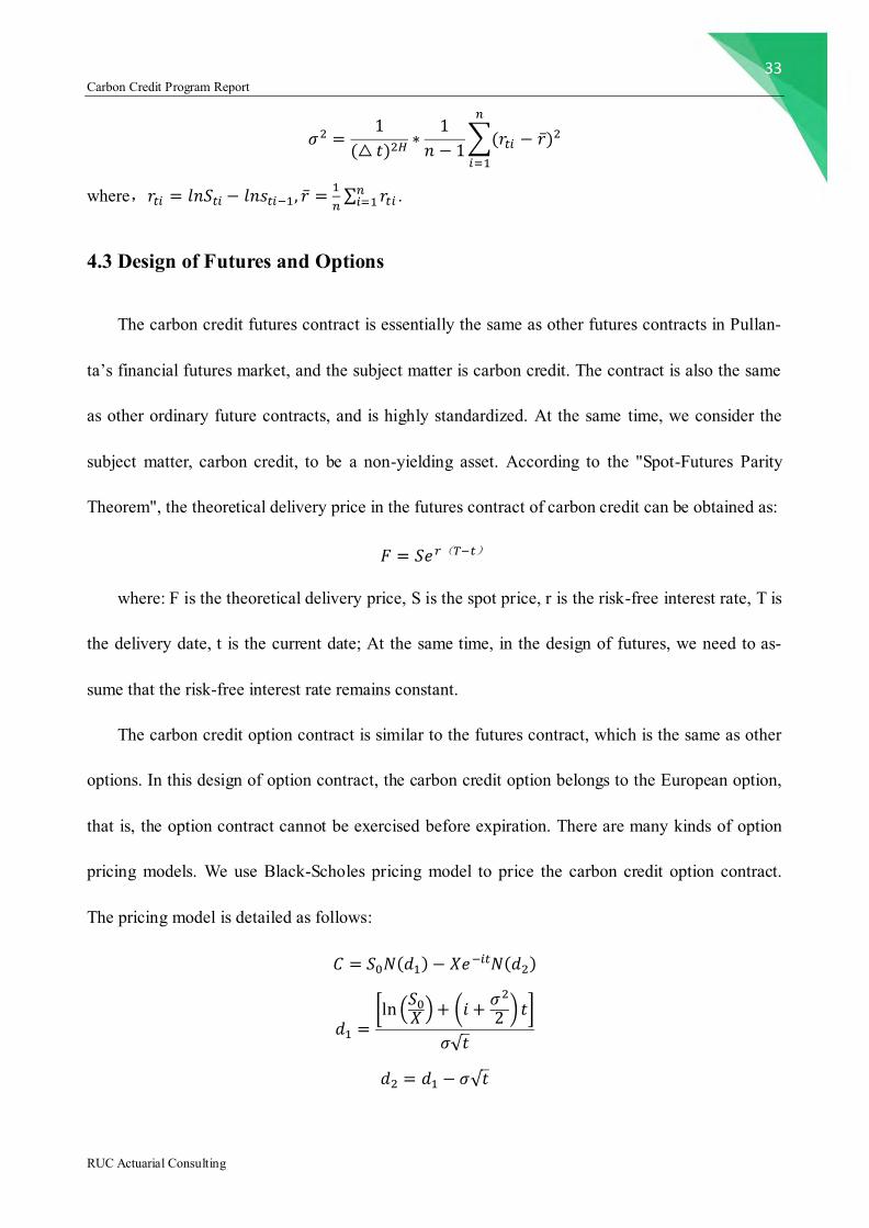
4.3 Design of Futures and Options
The carbon credit futures contract is essentially the same as other futures contracts in Pullan-
ta’s financial futures market, and the subject matter is carbon credit. The contract is also the same
as other ordinary future contracts, and is highly standardized. At the same time, we consider the
subject matter, carbon credit, to be a non-yielding asset. According to the "Spot-Futures Parity
Theorem", the theoretical delivery price in the futures contract of carbon credit can be obtained as:
𝐹 = 𝑆𝑒𝑟(𝑇−𝑡)
where: F is the theoretical delivery price, S is the spot price, r is the risk-free interest rate, T is
the delivery date, t is the current date; At the same time, in the design of futures, we need to as-
sume that the risk-free interest rate remains constant.
The carbon credit option contract is similar to the futures contract, which is the same as other
options. In this design of option contract, the carbon credit option belongs to the European option,
that is, the option contract cannot be exercised before expiration. There are many kinds of option
pricing models. We use Black-Scholes pricing model to price the carbon credit option contract.
The pricing model is detailed as follows:
𝐶 = 𝑆0𝑁(𝑑1) − 𝑋𝑒−𝑖𝑡𝑁(𝑑2)
𝑑1 =[ln (
𝑆0𝑋 )+ (𝑖 +
𝜎2
2 )𝑡]
𝜎√𝑡
𝑑2 = 𝑑1 − 𝜎√𝑡
34 Carbon Credit Program Report
RUC Actuarial Consulting
where: C is the price of the call option, S0 is the initial price of the subject matter, X is the
strike price, i is the risk-free interest rate, t is the length of the contract time, and is the standard
deviation of the change of the corresponding asset price;
4.4 Design of Bonds
4.4.1 Profit and loss structure of products
According to the calculation of the CER daily cash from 2011 to 2013, we know the average
price volatility reaches about 32%. It shows carbon spot prices are highly volatile. Therefore, the
bonds are designed to give investors the lowest return, that is, our products are guaranteed finan-
cial products. At the same time, in order to control financing costs and avoid excessive carbon
credits issuance, we set a ceiling for returns.
We design two bonds and both bonds pay interest at the end of each year. They are both
5-year spread-guaranteed bonds. Because 5 years is a key term in the term structure of interest
rates. They are:
①Bond A: a floating-rate carbon bond embedded in European bull spread options, which is
equivalent to a combination of 1 fixed-rate bond and 5 European bull spread options;
②Bond B: a floating-rate carbon bond embedded in Asian bull spread options, which is
equivalent to a combination of 1 fixed-rate bond and 5 Asian bull spread options. So bond B has a
strong path-dependent nature of the carbon spot price, which can reduce the impact of price fluc-
tuations to a certain extent.
The interest payment profit and loss charts of the two products in each period are similar, as
shown in Figures 3.3below.
s

35 Carbon Credit Program Report
RUC Actuarial Consulting
Figure 3.3. Bull spread & Fixed-rate bond & Spread-guaranteed bond
According the structure of bond A and B, we can write the formula of profit and loss at ma-
turity, consisting of two parts:
①the part of fixed income:
𝑃𝐵 =∑𝜂𝐵
(1 + 𝑖)𝑡+
𝐵
(1 + 𝑖)𝑇
𝑇
𝑡=1
②the part of floating income:
a. European bull spread option:
𝑃𝐶_𝑒𝑢𝑟𝑜 =
{
0, 𝑖𝑓 𝑆𝑡 < 𝑋1
𝐵 × 𝜃 (𝑆𝑡 − 𝑋1𝑆0
) , 𝑖𝑓 𝑋1 ≤ 𝑆𝑡 < 𝑋2 , 𝑡 = 1, …5
𝐵 × 𝜃 (𝑋2 − 𝑋1𝑆0
) , 𝑖𝑓 𝑆𝑡 ≥ 𝑋2
=𝐵 × 𝜃
𝑆0(max(𝑆𝑡 − 𝑋1 , 0) − max(𝑆𝑡 − 𝑋2, 0))
We set 𝐶1∗(𝑇) = max(𝑆𝑇 − 𝑋1 , 0),𝐶2∗(𝑇) = max(𝑆𝑇 − 𝑋2 , 0),to represent the value of two
embedded options at expiration.
b. Asian bull spread option:
𝑃𝐶_𝑎𝑠𝑖𝑎𝑛 =
{
0, 𝑖𝑓 𝐴𝑣𝑒𝑟𝑎𝑔𝑒𝑠𝑡 < 𝑋1
𝐵 × 𝜃 (𝐴𝑣𝑒𝑟𝑎𝑔𝑒𝑠𝑡 − 𝑋1
𝑆0) , 𝑖𝑓𝑋1 ≤ 𝐴𝑣𝑒𝑟𝑎𝑔𝑒𝑠𝑡 < 𝑋2 , 𝑡 = 1, … ,5
𝐵 × 𝜃 (𝑋2 − 𝑋1𝑆0
) , 𝑖𝑓𝐴𝑣𝑒𝑟𝑎𝑔𝑒𝑠𝑡 ≥ 𝑋2
The average value 𝐴𝑣𝑒𝑟𝑎𝑔𝑒𝑠𝑡 here is the average of the carbon spot prices at the end of each
month in each interest-paying year.
36 Carbon Credit Program Report
RUC Actuarial Consulting
In the formula above, B represents face value, 𝜂 is the principal guaranteed rate and 𝜃 rep-
resents the participation rate. 𝑋1,𝑋2 are the lower and upper limits of the price of the underlying
asset. The purpose of setting 𝜂 and θ here is to show that the product can be designed as a finan-
cial product.
4.4.2 Basic terms design of carbon bonds
The fixed-income characteristics of two bonds are achieved through the determination of
coupon rates. As for the parts linked to carbon spot price, we assume a group of European or Asian
bull spread options with carbon credit prices as the target are purchased.
4.4.2.1. Terms design of coupon bonds
Face value: B =100
Expiry date: T=5 year,and interest is paid once a year.
Coupon rate/ principal guaranteed rate:𝜂, that is, the 𝑓𝑎𝑐𝑒 𝑣𝑎𝑢𝑙𝑒 ∗ 𝜂 is paid as interest at
the end of each year.
Enforcement terms:it is not callable, not puttable and it can’t be converted into equity upon
maturity.
4.4.2.2 Terms design of options
Strike price:it is a call option. The parity method is adopted, which means the price of the
underlying asset on the product issue date is set as the strike price, that is,𝑋1 = 𝑆0 is set. This set-
ting can reflect the volatility value of options better. At the same time, suppose the maximum re-
turn limit of Pullanta’s financial products is 𝛿, we can set 𝑋2 = (1+ 𝛿) ∗ 𝑆0.
Underlying asset:the CER spot price of BlueNext Exchange
Because BlueNext Exchange is the largest CER trading market in the world and may have a
37 Carbon Credit Program Report
RUC Actuarial Consulting
great impact on the running of Pullanta’s carbon credits trading market, we set CER spot of
BlueNext Exchange as underlying asset. However, it should be noted that the price of CER is de-
nominated in Euro, and the bonds are issued in Pullanta and denominated in Pulo.
The basic terms of the carbon bonds are shown in table 4.3
Table4.3 Basic terms of carbon bonds
Coupon bonds Options
Face value:B=100 Strike price:X1=S0,X2=(1+δ)*S0
Expiry date:T=5year Underlying asset:carbon credits in exchange
Principal guaranteed rate: η Participation rate:θ
Non-callable, non-puttable, non-convertible, due to be executed at the expiry date;
The denomination currency is Pulo
4.4.3 Option valuation
In the options part, for Bond A- -the valuation of European floating-rate bond, the options
part is the sum of five bull spread options for one year, two years, three years, four years, and five
years. For Bond B--the Asian floating-rate bond, the options part involves the characteristics of
forward and path dependence, so it is necessary to use numerical simulation methods to value for-
ward options.
Combined with the foregoing, we use the European option pricing formula of the jump fractal
Brownian process to calculate the value of the options part. The calculation of Bond B is similar,
but some improvements need to be added.
4.4.3.1 Valuation process of European bull spread options
For European bull spread options, we only need to compare the relationship between the car-
bon spot price at the expiration date and the strike price to make a valuation.
38 Carbon Credit Program Report
RUC Actuarial Consulting
In the case that the carbon spot price obeys the geometric fractal Brownian motion, the fractal
BS formula can be used to calculate the value of the European bull spread option. Refer to the
fractal BS formula of the European call option at any time 𝑡 ∈ [0,𝑇] given by Necula (2002):
𝐶1∗(𝑡) = 𝑆𝑡𝑁(𝑑1) − 𝑋1𝑒
−𝑟𝑞(𝑇−𝑡)𝑁(𝑑2)
𝑑1 =ln(
𝑆𝑡𝑋1)+ 𝑟𝑞(𝑇 − 𝑡) +
12𝜎
2(𝑇2𝐻 − 𝑡2𝐻)
√𝑇2𝐻− 𝑡2𝐻𝜎
𝑑2 = 𝑑1 − √𝑇2𝐻 − 𝑡2𝐻𝜎
where 𝐶1∗(𝑡) = 𝐸𝑡∗(𝑒−𝑟𝑞(𝑇−𝑡)max (𝑆𝑇 − 𝑋1 , 0)), is the value of a standard Euro-denominated Eu-
ropean call option at time t.
Assuming that the Euro-Pulo exchange rate is independent of the carbon spot price, the value
of the two embedded options in carbon bonds can be calculated by the following formulas. Since
the pricing process of the two options 𝐶1(𝑡) and 𝐶2(𝑡) is similar, we just give the pricing for-
mula of option 1--𝐶1(𝑡) as an example. According to Hu and ksendal (2011), under the
risk-neutral measure, the current value of option 1--𝐶1(𝑡) is:
𝐶1(𝑡) = 𝐸𝑡∗ (𝑒−𝑟𝑓(𝑇−𝑡)𝐶1(𝑇)) =
𝐵𝜃
𝑆0𝑒(𝑟𝑞−𝑟𝑓)(𝑇−𝑡)𝐶1
∗(𝑡)
4.4.3.2 Valuation process of Asian bull spread options
For Asian floating-rate bonds, the payment of the floating-rate part of each period is not re-
lated to the carbon price on the date of interest payment, but to the average carbon price over the
entire floating-rate interval. Because such options have forward options and are path-dependent,
pricing should be approximated by numerical methods. With reference to Asmussen (1999), our
team uses Monte Carlo method to simulate the five-year carbon spot price under the fractal
Brownian motion, and then evaluates the Asian bull spread option. Specific steps are as follows:
a. assume that carbon spot price obeys the geometric fractal Brownian motion just like
39 Carbon Credit Program Report
RUC Actuarial Consulting
𝑑𝑙𝑛𝑆𝑡 = 𝑟𝑞𝑑𝑡 + 𝜎𝑑𝐵𝑡𝐻 − 𝜎2𝐻𝑡2𝐻−1𝑑𝑡,
then discretize Eulerian as:
Δ𝑙𝑛𝑆𝑡 = 𝑟𝑞Δ𝑡 + 𝜎Δ𝐵𝑡𝐻 − 𝜎2𝐻𝑡2𝐻−1Δ𝑡 (*)
Due to the incremental correlation of fractal Brownian motion, when the validity period of
claims is divided into n parts, using the autocorrelation feature of fractal Brownian motion, the
variance-covariance matrix between the increments of n fractal Brownian motion is:
Σ =1
2(Δ𝑡)2𝐻 {
𝐶11, 𝐶12 ,… , 𝐶1𝑛…
𝐶𝑛1, 𝐶𝑛2,… , 𝐶𝑛𝑛
}
𝑤ℎ𝑒𝑟𝑒 𝐶𝑖𝑗 = |𝑖 − 𝑗 + 1|2𝐻 + |𝑖 − 𝑗 − 1|2𝐻 − 2|𝑖 − 𝑗|2𝐻, 𝑖, 𝑗 = 1, … , 𝑛.
Therefore, an incremental random number of fractal Brownian motion on a path can be ob-
tained by extracting an n-dimensional joint normal distribution random number whose mean vec-
tor is 0 vector and variance-covariance matrix is Σ, and then obtain a path of carbon credits price
by recursion (*);
b. use Monte Carlo simulation method to generate enough (assuming 100,000) five-year carbon
credits price paths. For each path, take 60 observation points, that is, N = 60, then there are 12 ob-
servation points each year, △ 𝑡 = 𝑇/𝑁;
c. for each path, on the floating interest payment date at the end of each year, the arithmetic aver-
age of the carbon price of 12 observation points of the year is calculated. Then compare it with the
strike price, and then discount through the term structure of the Pulo’s risk-free interest rate to ob-
tain the Asian bull spread. So, a sample of the value of the option is obtained;
d. the arithmetic mean of the valuation of 100,000 paths is the valuation of the Asian bull spread
option.
40 Carbon Credit Program Report
RUC Actuarial Consulting
5.Social cost and government revenue
5.1 Social cost
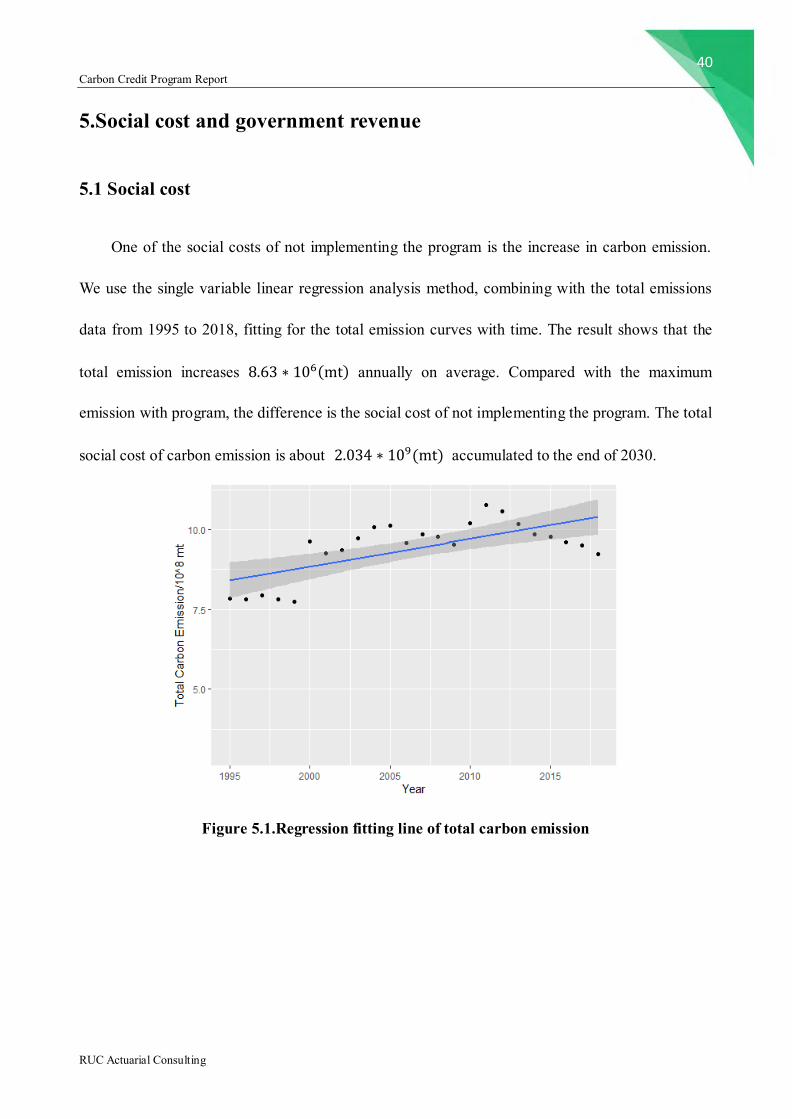
One of the social costs of not implementing the program is the increase in carbon emission.
We use the single variable linear regression analysis method, combining with the total emissions
data from 1995 to 2018, fitting for the total emission curves with time. The result shows that the
total emission increases 8.63 ∗ 106(mt) annually on average. Compared with the maximum
emission with program, the difference is the social cost of not implementing the program. The total
social cost of carbon emission is about 2.034 ∗ 109(mt) accumulated to the end of 2030.
Figure 5.1.Regression fitting line of total carbon emission
41 Carbon Credit Program Report
RUC Actuarial Consulting
Table 5.1 Social cost: Carbon emissions
Year Average emission
without program
Maximum emission
with program
difference
2018 922441064.3 922441064.3 0
2020 931070064.3 908604448.4 22465615.9
2021 939699064.3 890432359.4 49266704.9
2022 948328064.3 868171550.4 80156513.9
2023 956957064.3 842126403.9 114830660.4
2024 965586064.3 812651979.8 152934084.5
2025 974215064.3 780145900.6 194069163.7
2026 982844064.3 752840794 230003270.3
2027 991473064.3 730255570.2 261217494.1
2028 1000102064 711999181 288102883.3
2029 1008731064 697759197.3 310971867
2030 1017360064 687292809.4 330067254.9
Sum 2034085513
Enterprises may adopt two types of emission reduction measures: one is to reduce production,
and the other is to develop emission reduction technologies. The former has led to a reduction in
GDP, while the latter has led to an increase in the production costs of enterprises. Both are social
costs. It is difficult to predict the increased costs of enterprises due to the development of emission
reduction technologies, and it depends on the actual situation each year. The following is a forecast
of the increased social costs caused by the reduction of GDP.
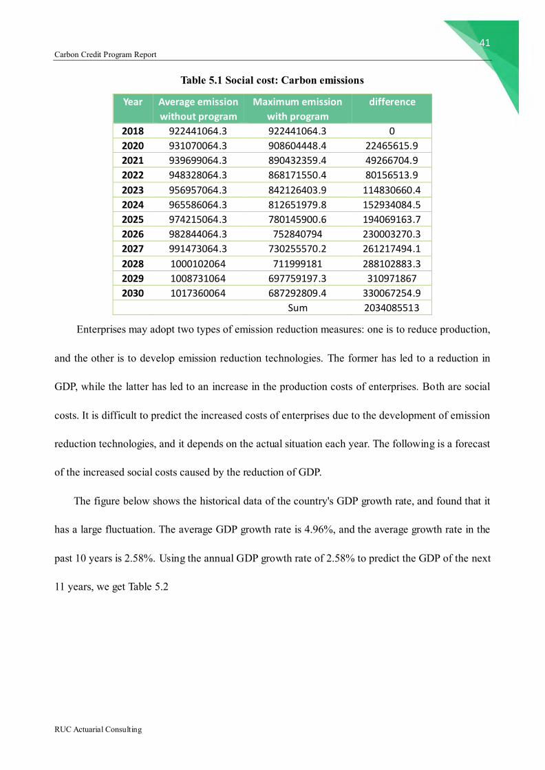
The figure below shows the historical data of the country's GDP growth rate, and found that it
has a large fluctuation. The average GDP growth rate is 4.96%, and the average growth rate in the
past 10 years is 2.58%. Using the annual GDP growth rate of 2.58% to predict the GDP of the next
11 years, we get Table 5.2
42 Carbon Credit Program Report
RUC Actuarial Consulting
Figure 5.2. GDP Growth Rate from 1996 to 2019
Table 5.2 Social cost: the reduction of GDP
Year GDP without program GDP with program Difference
2020 744471634445 757341830908 12870196463
2021 763679002613 766651759174 2972756561
2022 783381920881 777412343526 -5969577355
2023 803593174440 789505584888 -14087589552
2024 824325878340 802800088211 -21525790129
2025 845593486001 817153459639 -28440026362
2026 867409797940 828054467486 -39355330454
2027 889788970727 836866115506 -52922855221
2028 912745526172 843739200990 -69006325182
2029 936294360747 848790918772 -87503441975
2030 960450755254 852396991551 -1.08054E+11
Total -4.11022E+11
By the end of 2030, the country's total GDP reduction due to the implementation of emission
reduction program is expected to be -4.11022E + 11.
43 Carbon Credit Program Report
RUC Actuarial Consulting
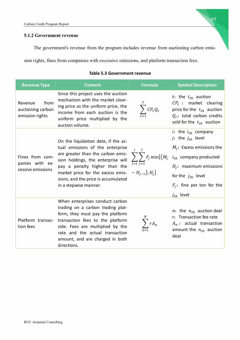
5.1.2 Government revenue
The government's revenue from the program includes revenue from auctioning carbon emis-
sion rights, fines from companies with excessive emissions, and platform transaction fees.
Table 5.3 Government revenue
Revenue Type Content Formula Symbol Description
Revenue from
auctioning carbon
emission rights
Since this project uses the auction
mechanism with the market clear-
ing price as the uniform price, the
income from each auction is the
uniform price multiplied by the
auction volume.
∑𝐶𝑃𝑡𝑄𝑡
𝑇
𝑡=1
t:the 𝑡𝑡ℎ auction
𝐶𝑃𝑡 : market clearing
price for the 𝑡𝑡ℎ auction
𝑄𝑡:total carbon credits
sold for the 𝑡𝑡ℎ auction
Fines from com-
panies with ex-
cessive emissions
On the liquidation date, if the ac-
tual emissions of the enterprise
are greater than the carbon emis-
sion holdings, the enterprise will
pay a penalty higher than the
market price for the excess emis-
sions, and the price is accumulated
in a stepwise manner.
∑∑𝐹𝑗min{(𝑀𝑗
𝐽
𝑗=1
𝐼
𝑖=1
−𝐻𝑗−1), 𝐻𝑗}
i:the 𝑖𝑡ℎ company
j:the 𝑗𝑡ℎ level
𝑀𝑗:Excess emissions the
𝑖𝑡ℎ company producted
𝐻𝑗:maximum emissions
for the 𝑗𝑡ℎ level
𝐹𝑗:fine per ton for the
𝑗𝑡ℎ level
Platform transac-
tion fees
When enterprises conduct carbon
trading on a carbon trading plat-
form, they must pay the platform
transaction fees to the platform
side. Fees are multiplied by the
rate and the actual transaction
amount, and are charged in both
directions.
∑𝑟𝐴𝑛
𝑁
𝑛=1
n:the 𝑛𝑡ℎ auction deal
r:Transaction fee rate
𝐴𝑛 : actual transaction
amount the 𝑛𝑡ℎ auction
deal
44 Carbon Credit Program Report
RUC Actuarial Consulting
6. Sensitivity Analysis
The emission reduction plan used in the case in the third part of this article is a three-stage
emission reduction. The intensity of emission reduction increases first and then decreases. It is
formulated by predicting the development of emission reduction technology in Pullanta in the fu-
ture. If the development status does not meet our assumptions, the emission reduction plan will
change accordingly, and the following four plans (including one used in this article) will be ana-
lyzed for sensitivity.
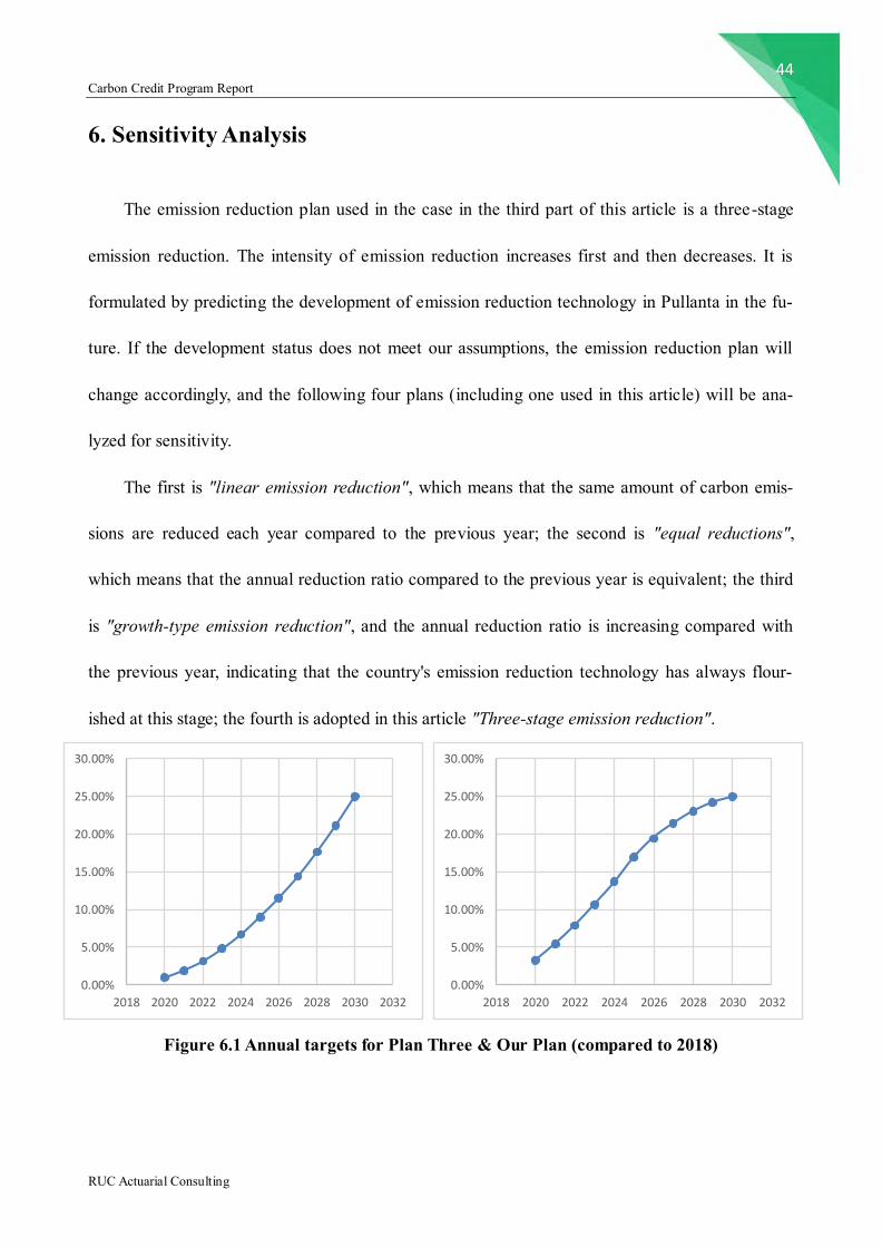
The first is "linear emission reduction", which means that the same amount of carbon emis-
sions are reduced each year compared to the previous year; the second is "equal reductions",
which means that the annual reduction ratio compared to the previous year is equivalent; the third
is "growth-type emission reduction", and the annual reduction ratio is increasing compared with
the previous year, indicating that the country's emission reduction technology has always flour-
ished at this stage; the fourth is adopted in this article "Three-stage emission reduction".
Figure 6.1 Annual targets for Plan Three & Our Plan (compared to 2018)
0.00%
5.00%
10.00%
15.00%
20.00%
25.00%
30.00%
2018 2020 2022 2024 2026 2028 2030 2032
0.00%
5.00%
10.00%
15.00%
20.00%
25.00%
30.00%
2018 2020 2022 2024 2026 2028 2030 2032
45 Carbon Credit Program Report
RUC Actuarial Consulting
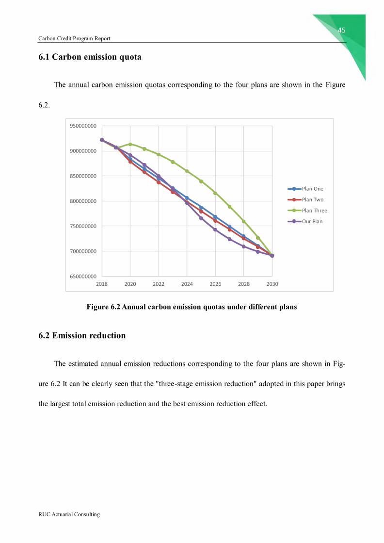
6.1 Carbon emission quota
The annual carbon emission quotas corresponding to the four plans are shown in the Figure
6.2.
Figure 6.2 Annual carbon emission quotas under different plans
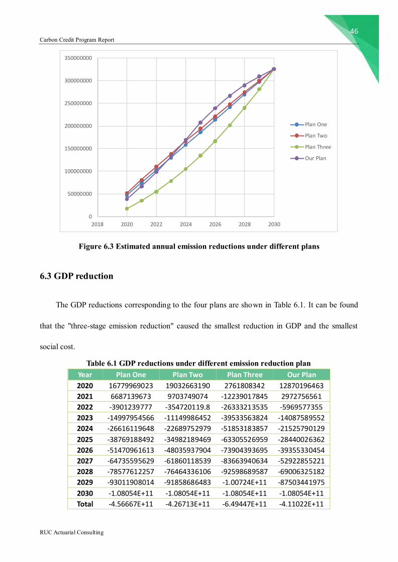
6.2 Emission reduction
The estimated annual emission reductions corresponding to the four plans are shown in Fig-
ure 6.2 It can be clearly seen that the "three-stage emission reduction" adopted in this paper brings
the largest total emission reduction and the best emission reduction effect.
650000000
700000000
750000000
800000000
850000000
900000000
950000000
2018 2020 2022 2024 2026 2028 2030
Plan One
Plan Two
Plan Three
Our Plan
46 Carbon Credit Program Report
RUC Actuarial Consulting
Figure 6.3 Estimated annual emission reductions under different plans
6.3 GDP reduction
The GDP reductions corresponding to the four plans are shown in Table 6.1. It can be found
that the "three-stage emission reduction" caused the smallest reduction in GDP and the smallest
social cost.
Table 6.1 GDP reductions under different emission reduction plan Year Plan One Plan Two Plan Three Our Plan
2020 16779969023 19032663190 2761808342 12870196463
2021 6687139673 9703749074 -12239017845 2972756561
2022 -3901239777 -354720119.8 -26333213535 -5969577355
2023 -14997954566 -11149986452 -39533563824 -14087589552
2024 -26616119648 -22689752979 -51853183857 -21525790129
2025 -38769188492 -34982189469 -63305526959 -28440026362
2026 -51470961613 -48035937904 -73904393695 -39355330454
2027 -64735595629 -61860118539 -83663940634 -52922855221
2028 -78577612257 -76464336106 -92598689587 -69006325182
2029 -93011908014 -91858686483 -1.00724E+11 -87503441975
2030 -1.08054E+11 -1.08054E+11 -1.08054E+11 -1.08054E+11
Total -4.56667E+11 -4.26713E+11 -6.49447E+11 -4.11022E+11
0
50000000
100000000
150000000
200000000
250000000
300000000
350000000
2018 2020 2022 2024 2026 2028 2030
Plan One
Plan Two
Plan Three
Our Plan
47 Carbon Credit Program Report
RUC Actuarial Consulting
It is not difficult to see from the sensitivity analysis that the "three-stage emission reduction"
plan is effective.
7. Risks and Alternatives
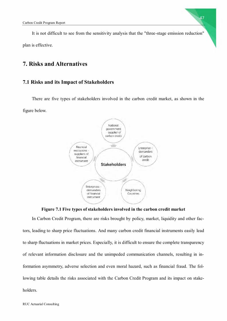
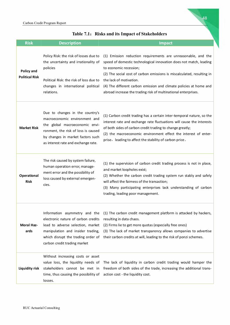
7.1 Risks and its Impact of Stakeholders
There are five types of stakeholders involved in the carbon credit market, as shown in the
figure below.
Figure 7.1 Five types of stakeholders involved in the carbon credit market
In Carbon Credit Program, there are risks brought by policy, market, liquidity and other fac-
tors, leading to sharp price fluctuations. And many carbon credit financial instruments easily lead
to sharp fluctuations in market prices. Especially, it is difficult to ensure the complete transparency
of relevant information disclosure and the unimpeded communication channels, resulting in in-
formation asymmetry, adverse selection and even moral hazard, such as financial fraud. The fol-
lowing table details the risks associated with the Carbon Credit Program and its impact on stake-
holders.
48 Carbon Credit Program Report
RUC Actuarial Consulting
Table 7.1:Risks and its Impact of Stakeholders
Risk Description Impact
Policy and
Political Risk
Policy Risk: the risk of losses due to
the uncertainty and irrationality of
policies
Political Risk: the risk of loss due to
changes in international political
relations.
(1) Emission reduction requirements are unreasonable, and the
speed of domestic technological innovation does not match, leading
to economic recession;
(2) The social cost of carbon emissions is miscalculated, resulting in
the lack of motivation.
(4) The different carbon emission and climate policies at home and
abroad increase the trading risk of multinational enterprises.
Market Risk
Due to changes in the country's
macroeconomic environment and
the global macroeconomic envi-
ronment, the risk of loss is caused
by changes in market factors such
as interest rate and exchange rate.
(1) Carbon credit trading has a certain inter-temporal nature, so the
interest rate and exchange rate fluctuations will cause the interests
of both sides of carbon credit trading to change greatly;
(2) the macroeconomic environment effect the interest of enter-
prise,leading to affect the stability of carbon price。
Operational
Risk
The risk caused by system failure,
human operation error, manage-
ment error and the possibility of
loss caused by external emergen-
cies.
(1) the supervision of carbon credit trading process is not in place,
and market loopholes exist;
(2) Whether the carbon credit trading system run stably and safely
will affect the fairness of the transaction;
(3) Many participating enterprises lack understanding of carbon
trading, leading poor management.
Moral Haz-
ards
Information asymmetry and the
electronic nature of carbon credits
lead to adverse selection, market
manipulation and insider trading,
which disrupt the trading order of
carbon credit trading market
(1) The carbon credit management platform is attacked by hackers,
resulting in data chaos.
(2) Firms lie to get more quotas (especially free ones)
(3) The lack of market transparency allows companies to advertise
their carbon credits at will, leading to the risk of ponzi schemes.
Liquidity risk
Without increasing costs or asset
value loss, the liquidity needs of
stakeholders cannot be met in
time, thus causing the possibility of
losses.
The lack of liquidity in carbon credit trading would hamper the
freedom of both sides of the trade, increasing the additional trans-
action cost - the liquidity cost.
49 Carbon Credit Program Report
RUC Actuarial Consulting
Without a carbon credit program, society will face the risk of global warming, increased
global desertification and declining biodiversity caused by carbon emissions. The cost of these
risks will be non-financial.
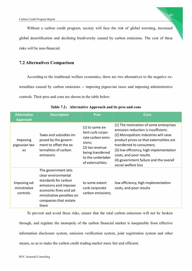
7.2 Alternatives Comparison
According to the traditional welfare economics, there are two alternatives to the negative ex-
ternalities caused by carbon emissions -- imposing pigouvian taxes and imposing administrative
controls. Their pros and cons are shown in the table below:
Table 7.2:Alternative Approach and its pros and cons
Alternative
Approach
Description Pros Cons
Imposing
pigouvian tax-
es
Taxes and subsidies im-
posed by the govern-
ment to offset the ex-
ternalities of carbon
emissions
(1) to some ex-
tent curb corpo-
rate carbon emis-
sions;
(2) tax revenue
being transferred
to the undertaker
of externalities.
(1) The motivation of some enterprises
emission reduction is insufficient;
(2) Monopolistic industries will raise
product prices so that externalities are
transferred to consumers;
(3) low efficiency, high implementation
costs, and poor results
(4) government failure and the overall
social welfare loss
Imposing ad-
ministrative
controls.
The government sets
clear environmental
standards for carbon
emissions and imposes
economic fines and ad-
ministrative penalties on
companies that violate
them
to some extent
curb corporate
carbon emissions;
low efficiency, high implementation
costs, and poor results
To prevent and avoid these risks, ensure that the total carbon emissions will not be broken
through, and regulate the monopoly of the carbon financial market is inseparable from effective
information disclosure system, emission verification system, joint registration system and other
means, so as to make the carbon credit trading market more fair and efficient.
50 Carbon Credit Program Report
RUC Actuarial Consulting
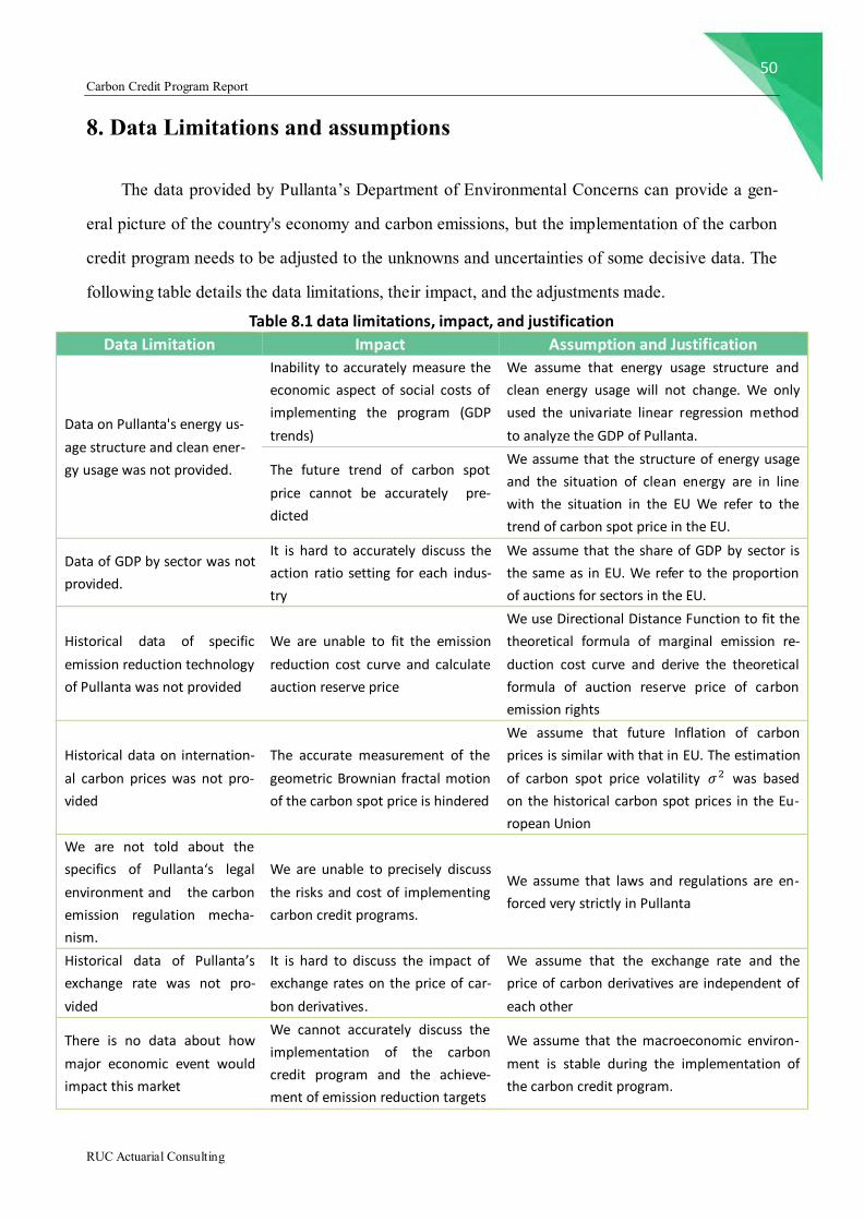
8. Data Limitations and assumptions
The data provided by Pullanta’s Department of Environmental Concerns can provide a gen-
eral picture of the country's economy and carbon emissions, but the implementation of the carbon
credit program needs to be adjusted to the unknowns and uncertainties of some decisive data. The
following table details the data limitations, their impact, and the adjustments made.
Table 8.1 data limitations, impact, and justification
Data Limitation Impact Assumption and Justification
Data on Pullanta's energy us-
age structure and clean ener-
gy usage was not provided.
Inability to accurately measure the
economic aspect of social costs of
implementing the program (GDP
trends)
We assume that energy usage structure and
clean energy usage will not change. We only
used the univariate linear regression method
to analyze the GDP of Pullanta.
The future trend of carbon spot
price cannot be accurately pre-
dicted
We assume that the structure of energy usage
and the situation of clean energy are in line
with the situation in the EU We refer to the
trend of carbon spot price in the EU.
Data of GDP by sector was not
provided.
It is hard to accurately discuss the
action ratio setting for each indus-
try
We assume that the share of GDP by sector is
the same as in EU. We refer to the proportion
of auctions for sectors in the EU.
Historical data of specific
emission reduction technology
of Pullanta was not provided
We are unable to fit the emission
reduction cost curve and calculate
auction reserve price
We use Directional Distance Function to fit the
theoretical formula of marginal emission re-
duction cost curve and derive the theoretical
formula of auction reserve price of carbon
emission rights
Historical data on internation-
al carbon prices was not pro-
vided
The accurate measurement of the
geometric Brownian fractal motion
of the carbon spot price is hindered
We assume that future Inflation of carbon
prices is similar with that in EU. The estimation
of carbon spot price volatility 𝜎2 was based
on the historical carbon spot prices in the Eu-
ropean Union
We are not told about the
specifics of Pullanta‘s legal
environment and the carbon
emission regulation mecha-
nism.
We are unable to precisely discuss
the risks and cost of implementing
carbon credit programs.
We assume that laws and regulations are en-
forced very strictly in Pullanta
Historical data of Pullanta’s
exchange rate was not pro-
vided
It is hard to discuss the impact of
exchange rates on the price of car-
bon derivatives.
We assume that the exchange rate and the
price of carbon derivatives are independent of
each other
There is no data about how
major economic event would
impact this market
We cannot accurately discuss the
implementation of the carbon
credit program and the achieve-
ment of emission reduction targets
We assume that the macroeconomic environ-
ment is stable during the implementation of
the carbon credit program.
51 Carbon Credit Program Report
RUC Actuarial Consulting
9. Conclusion
Based on the analysis and model construction above, we can believe that the carbon credit
program above can complete the emission reduction plan of the Department of Environmental
Concerns of Pullanta, and can provide revenue for the government during the emission reduction
process, promote the diversity and liquidity of the financial market of Pullanta. We model carbon
credit price by using the jump fractional Brownian process, and use ‘Marginal Abatement Cost
Pricing Model’ to construct the auction market of carbon credit. Meanwhile, secondary market
construction are adopted in this plan to ensure the normal operation of Pullanta's carbon credit
market. However, there are still some limitations in the formulation of this plan, which still needs
to be adjusted according to the actual situation of Pullanta and the implementation of the plan.
52 Carbon Credit Program Report
RUC Actuarial Consulting
10. References
[1] Pauline Barrieu & Max Fehr. (2011). Integrated EUA and CER price modeling and appli-
cation for spread option pricing. Retrieved from https: //ssrn.lom/abstract=1737637.
[2] Hurst H. (1951). Long term storage capacity of reservoirs .Transactions of the American Soci-
ety of Civil Engineers, 116,770-799.
[3] George Daskalakis. & Raphael N. Markellos. (2008). are the European carbon market effi-
cient[J] . Review of Futures Markets,17(2),103-128.
[4] Ciprian Necula. (2002) Option Pricing in a Fractional Brownian Motion Environment. Acade-
my of Economic Studies Bucharest, Romania.
[5] Pauline Barrieu & Max Fehr (2011), Integrated EUA and CER Price Modeling and Applica-
tion for Spread Option Pricing. working paper.
[6] S. Asmussen. (1999),Stochastic Simulation with a View Towards Stochastic Processes. Notes
of a Concentrated Advance Course at MaPhySto, Aarhus Denmark, 2
[6] Dutschkea. Metal. (2004). Value and Risks of Expiring Carbon Credits from CDM Afforesta-
tion and Reforestation HWWA Discussion Paper. 290.
[7] Seifert, J. Uhrig-Homburg, M. & Wagner, M. (2008). Dynamic behavior of co2 spot prices.
Journal of Environmental Economics and Management, 56.
[8] Labatt, S., & White, R. R. (2015). Carbon Finance: The Financial Implications of Climate
Change.
[9] The Wrong Sort of Recycling, THE ECONOMIST. (2010, Mar. 25). Retrieved Feb 21, 2020,
from http: / /www. economist. com /node /15774368.
53 Carbon Credit Program Report
RUC Actuarial Consulting
[10] Michael Szabo. (2008, Dec 2). DNV Suspension Another Jab at Battered CO2 Scheme,
REUTERS, Retrieved Feb 21, 2020, from http: / /www. reuters. com /article /2008 /12 /02 /us -
carbon - dnv - idUSTRE4B04K120081202.
[11] Mark Schapiro. (2010). Conning the Climate: Inside the Carbon Trading Shell Game.
Harper's Magazine,21, 31-39
[12]Zheng, Y.H.(2016). Tan jinrong shichang de dingjia yu jiage yunxing jizhi yanjiu [Research on
the Pricing Mechanism and Price Operation Mechanism of Carbon Financial Market]. Zhongguo
kuangye daxue(Beijing)
[13]Feng, J.F. & Xia, C.X. & Wang, C.X.(2018). Tan paifang quan jiage jianmo yu tan zhaiquan
guzhi. [Carbon Emission Right Price Modeling and Carbon Bond Valuation]. Hebei jingmao daxue
xuebao, 39(01), 66-72.
[14]Gao, S. & Li, M.Y. & Duan, M.S. et al.(2019). Bali Xieding xia de guoji tan shichang jizhi:
jiben xingshi he qianjing zhanwang. [International market mechanisms under Paris Agreement:
basic form and future prospects]. Qihou bianhua yanjiu jinzhan, 15 (3), 222-231
[15] Chen, J.M. & Li H.D. & Wang, X.S.(2013). Aodaliya tan paifang jiaoyi tixi de tese fenxi ji
qishi. [Characteristics Analysis and Enlightenment of Carbon Emission Trading System in Aus-
tralia].Shengtai jingji, 04, 70-74+87.
[16]Feng, J.F. & Chen, J. & Du, D.Y. & Liu, Q.M.(2015). Tan zhaiquan de guzhi ji minganxing
fenxi. [Carbon Bond Pricing and Sensitivity Analysis]. Kexue juece, 10, 17-32.
[17]Zhang, Y. & Li, Y. (2018). Guoji tan paifang quan jiaoyi tixi yanjiu ji dui zhongguo de qishi.
[Research on the International Carbon Emission Trading Scheme and Its Implications to China].
Shengtai jingji, 34(02):66-70.
54 Carbon Credit Program Report
RUC Actuarial Consulting
[18]Chen, N. & Lian, N.N. (2019). Qianxi woguo tan paifangquan jiaoyi shichang youhua
lujing——jiyu tan paifangquan jiage shijiao. [Analysis on Optimized Path to Trading Market of
Carbon Emission in China——from the price perspective of carbon emission rights]. Hunan
shewai jingji xueyuan xuebao, 19(03):35-44.
[19] Onno Kuik, Luke Brander & Richard S.J. Tol. (2009). Marginal abatement costs of green-
house gas emissions: A meta-analysis. Energy policy, 37(4): 1395-1403.
[20] Liao, C., H. & Onal, M. H. Chen. (2009). Average shadow price and equilibrium price: case
study of tradable pollution permit markets. European Journal of Operational Research,
196(3):1207-1213.
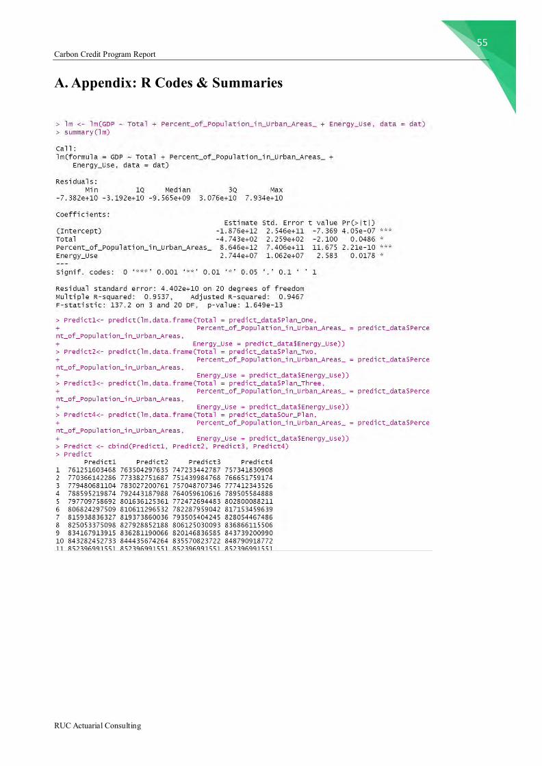
55 Carbon Credit Program Report
RUC Actuarial Consulting
A. Appendix: R Codes & Summaries
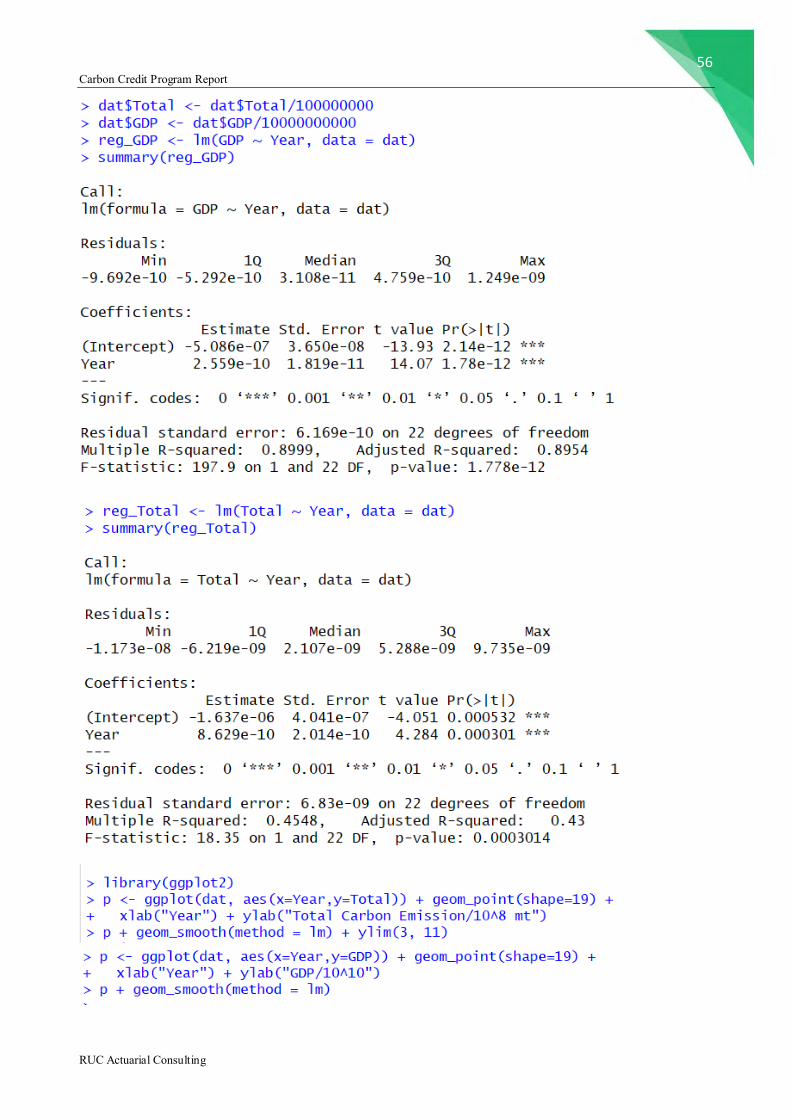
56 Carbon Credit Program Report
RUC Actuarial Consulting