Embed Size (px)
Citation preview
Carbon Dioxide Emission Pathways Avoiding Dangerous Ocean Impacts
K. KVALE* AND K. ZICKFELD1
University of Victoria, Victoria, British Columbia, Canada
T. BRUCKNER
Institute for Infrastructure and Resources Management, University of Leipzig, Leipzig, Germany
K. J. MEISSNER
University of Victoria, Victoria, British Columbia, Canada
K. TANAKA
International Institute for Applied Systems Analysis, Laxenburg, Austria, Center for International Climate and Environmental
Research, Oslo, Norway, and Institute for Atmospheric and Climate Science, ETH Zurich, Zurich, Switzerland
A. J. WEAVER
University of Victoria, Victoria, British Columbia, Canada
(Manuscript received 26 July 2011, in final form 21 June 2012)
ABSTRACT
Anthropogenic emissions of greenhouse gases could lead to undesirable effects on oceans in coming centuries.
Drawing on recommendations published by the German Advisory Council on Global Change, levels of un-
acceptable global marine change (so-called guardrails) are defined in terms of global mean temperature, sea level
rise, and ocean acidification. A global-mean climate model [the Aggregated Carbon Cycle, Atmospheric
Chemistry andClimateModel (ACC2)] is coupledwith an economicmodule [taken from theDynamic Integrated
Climate–EconomyModel (DICE)] to conduct a cost-effectiveness analysis to derive CO2 emission pathways that
both minimize abatement costs and are compatible with these guardrails. Additionally, the ‘‘tolerable windows
approach’’ is used to calculate a range of CO2 emissions paths that obey the guardrails as well as a restriction on
mitigation rate. Prospects of meeting the global mean temperature change guardrail (28 and 0.28C decade21
relative to preindustrial) depend strongly on assumed values for climate sensitivity: at climate sensitivities .38Cthe guardrail cannot be attained under any CO2 emissions reduction strategy without mitigation of non-CO2
greenhouse gases. The ocean acidification guardrail (0.2 unit pH decline relative to preindustrial) is less restrictive
than the absolute temperature guardrail at climate sensitivities .2.58C but becomes more constraining at lower
climate sensitivities. The sea level rise and rate of rise guardrails (1 m and 5 cm decade21) are substantially less
stringent for ice sheet sensitivities derived in the Intergovernmental Panel on Climate Change (IPCC) Fourth
Assessment Report, but they may already be committed to violation if ice sheet sensitivities consistent with
semiempirical sea level rise projections are assumed.
1. Introduction
As the body of knowledge grows regarding the pos-
sible worsening effects of an increasingly altered climate
state, so too do concerns over how to avoid the most
drastic outcomes. Intergovernmental collaboration on
this topic was proclaimed by Article 2 of the United
Nations Framework Convention on Climate Change
(UNFCCC), which calls for the avoidance of ‘‘dangerous
* Current affiliation: Climate Change Research Centre, Univer-
sity of New South Wales, Sydney, New South Wales, Australia.1Current affiliation: Department of Geography, Simon Fraser
University, Burnaby, British Columbia, Canada.
Corresponding author address: Karin Kvale, Climate Change
Research Centre, Level 4 Mathews Building, University of New
South Wales, Sydney, NSW 2052, Australia.
E-mail: [email protected]
212 WEATHER , CL IMATE , AND SOC IETY VOLUME 4
DOI: 10.1175/WCAS-D-11-00030.1
� 2012 American Meteorological Society
anthropogenic interference with the climate system’’
(UNFCCC 1992). Clearly any definition of ‘‘dangerous
anthropogenic interference’’ (DAI) involves a value
judgment as perceptions of danger vary among individuals
and social groups (Dessai et al. 2004). Such value judg-
ments are ideally excluded from scientific analysis, so
quantitative studies often address Article 2 obliquely,
such as via risk or vulnerability assessments [e.g., ‘‘rea-
sons for concern,’’ ‘‘concepts of danger,’’ or ‘‘key vul-
nerabilities,’’ terms used respectively in Smith et al.
(2001); ECF (2004), and Schneider et al. 2007], and leave
to policymakers the task of determining what is ac-
ceptable. In an alternative approach, thresholds for DAI
are defined based on expert judgments of systemic
physical, ecological, or societal tolerances (e.g., Parry
et al. 2001; O’Neill and Oppenheimer 2002; Barnett and
Adger 2003; Corfee-Morlot and Hohne 2003; Graßl
et al. 2003; Oppenheimer and Alley 2004; Hansen 2005;
Keller et al. 2005; Schubert et al. 2006; Harvey 2007;
Funk et al. 2008). Despite varied approaches and per-
spectives, general consensus suggests that common
definitions of danger include singular events with irre-
versible and widespread consequences that have been
referred to as ‘‘tipping points’’ in the recent literature
(Lenton et al. 2007; e.g., collapse of the thermohaline
circulation, disintegration of one or both polar ice sheets)
and lasting conditions with broad ecological and eco-
nomic impacts (e.g., widespread and frequent coral reef
bleaching, rapid sea level rise, increased frequency of
extreme weather). The European Union has settled
upon a precautionary 28C target for avoiding the most
dangerous impacts, a target that is now supported by
numerous scientific and environmental groups and most
nations on Earth (e.g., Graßl et al. 2003; Bali Declaration
2007; Union of Concerned Scientists 2007; Greenpeace
2008; Copenhagen Accord 2009).
What avoiding DAI implies in terms of greenhouse
gas (GHG) emissions can be explored through the use of
integrated assessment models including relevant social
and environmental aspects. A number of climatic thresh-
olds (e.g., global mean temperature, thermohaline circu-
lation stability) have been used to calculate least-cost
emissions pathways (e.g., Keller et al. 2000;Mastrandrea
and Schneider 2004; Keller et al. 2005; Bruckner and
Zickfeld 2009; McInerney and Keller 2008). Emissions
corridors compatible with such thresholds can also be
calculated using the ‘‘tolerable windows approach’’
(TWA; Bruckner et al. 1999; Petschel-Held et al. 1999).
Corridors define a solution space for emissions pathways
that satisfy prescribed constraints or ‘‘guardrails.’’ Emis-
sions corridors constrained simultaneously by environ-
mental and economic considerations have been calculated
by Petschel-Held et al. (1999) and Kriegler and Bruckner
(2004) for global mean temperature guardrails, by Toth
et al. (2003) for degree of ecological transformation, and
by Zickfeld and Bruckner (2003, 2008) and Bruckner and
Zickfeld (2009) for thermohaline circulation stability.
Because of their societal importance, climatic thresh-
olds other than global mean temperature and thermoha-
line circulation merit examination using the above
approaches. Sea level rise threatens a growing proportion
of the world population as coastal cities expand; a 40-cm
rise in mean sea level by the 2080s could flood 100 million
people per year for even low emission Special Report on
Emissions (SRES) scenarios (Nakicenovic et al. 2000),
assuming no additional flood defenses are put in place
(Nicholls et al. 2007). Globally ocean pH has decreased
0.1 units from the average acidity in 1750 (Orr et al. 2005),
with a continuing decline expected to have detrimental
consequences for marine life that has evolved in a
slightly alkaline and relatively stable chemical environ-
ment. A decrease in seawater pH lowers the saturation
state for carbonate minerals such as calcite and arago-
nite. This affects the stability and production rates of
carbonate minerals, which are the building blocks of
coral reefs and form the shells and skeletons of other
marine calcifying organisms. Coral reefs contain 25%
of marine species (Buddemeier et al. 2004) and supply
2%–5% of the annual global fisheries harvest (Fischlin
et al. 2007), mostly in developing nations (Pauly et al.
2005). Using ocean acidity as a threshold for allowable
carbon emissions was recently suggested to be critical
but utterly lacking (Zeebe et al. 2008). Because ocean
acidification is largely dependent on carbon dioxide
(with minimal dependence on temperature), application
of an ocean acidification threshold is essentially equiv-
alent to setting a CO2 concentration target.
Cost-effective pathways and emissions corridors are
derived here using a set of indicators for undesirable
climate changes (global mean temperature change, sea
level rise, and ocean acidification) to constrain future
CO2 emissions pathways.
These so-called guardrails were published by the
German Advisory Council on Global Change (WBGU;
Schubert et al. 2006) and are to be interpreted as rec-
ommended boundaries on acceptable levels of anthro-
pogenic alteration of the Earth system, for the purpose
of giving decision makers quantitative guidelines for
avoiding DAI. The set of guardrails is as follows (in the
following referred to as ‘‘WBGU guardrails’’):
d Climate protection: The globalmean rise in near-surface
air temperature must be limited to a maximum of 28Crelative to the preindustrial value while also limiting the
rate of temperature change to a maximum of 0.28Cdecade21 (originally proposed in Graßl et al. 2003).
JULY 2012 KVALE ET AL . 213
d Sea level rise: Absolute sea level rise should not
exceed 1 m in the long term (implied to be steady
state in the document), and the rate should remain
below 5 cm decade21 at all times.d Ocean acidification: The pH of near-surface water
should not drop more than 0.2 units below the pre-
industrial average value in any larger ocean region
(nor in the global mean).
The absolute guardrails reflect both human and envi-
ronmental limits of intolerable change, while the rate
guardrails reflect the maximum estimated rates of hu-
man and environmental adaptive capacity. The WBGU
report (Schubert et al. 2006) also recommends a pro-
tection of 20%–30% of the area of marine ecosystems
and mentions the risk of triggering the release of
methane hydrate under global warming, but these issues
are not addressed in this study. The WBGU guardrails
are used as constraints in a coupled climate–economy
model to calculate least-cost emissions pathways and
emissions corridors.
2. Methods
A globally averaged climate–carbon cycle model, the
Aggregated Carbon Cycle, Atmospheric Chemistry and
Climate Model (ACC2 3.1; Tanaka et al. 2007; Tanaka
2008), is coupled with a simple model of the world econ-
omy, based on the economic module in the Dynamic
Integrated Climate–Economy Model (DICE; Nordhaus
1992, 1994; Nordhaus and Boyer 2000; Nordhaus 2008),
in order to assess the social mitigation burden associated
with time-dependent emissions mitigation efforts. The
sea level component of ACC2 ismodified to improve the
representation of thermal expansion and the sea level
rise contribution from ice caps and small glaciers, and to
reflect new estimates of the mass balance sensitivity of
the Greenland and Antarctic ice sheets. A detailed de-
scription of the modifications made to the thermal ex-
pansion and sea level rise calculations in ACC2 can be
found in the appendix. The DICE version used is DICE-
2007, which is described in Nordhaus (2008).
a. Model ACC2
The model ACC2 (Tanaka 2008) describes major
physical and biogeochemical processes in the Earth
system on a global-annual-mean level.1 ACC2 is a de-
scendant of the Integrated Assessment of Climate Pro-
tection Strategies (ICLIPS) Climate Model (ICM)
(Bruckner et al. 2003) and has been used for several
applications (e.g., Tanaka et al. 2009a,b; Tanaka and
Raddatz 2011). Ocean and land CO2 uptake are de-
scribed by two separate four-reservoir box models
tuned to the respective impulse response functions, which
are the measured temporal response of a state variable
calculated from the perturbation of the control run of a
more complex model (Hooss et al. 2001; Joos et al.
1996). Parameterizations of atmospheric chemistry involve
direct radiative forcing agents (CO2, CH4, N2O, SF6, 29
species of halocarbons, tropospheric and stratospheric
O3, and stratospheric water vapor) and indirect radiative
forcing agents (OH, NOx, CO, and VOC) (Joos et al.
2001). The radiative forcing due to aerosols is repre-
sented by the following three types: the direct effect
of sulfate aerosols, the direct effect of carbonaceous
aerosols (black carbon and organic carbon), and the
indirect effect of all aerosols. The sum of the individual
radiative forcing terms is the total radiative forcing,
which is used by an energy balance model, the Diffusion
Ocean Energy Balance Climate Model (DOECLIM;
Kriegler 2005) to calculate surface air temperature.
DOECLIM comprises essentially two boxes: 1) land
coupled with the troposphere over land and 2) ocean
coupled with the troposphere over ocean. Coupled to
the ocean box is a heat diffusion model that describes
heat transfer to the deep ocean, which is described in
greater detail in Tanaka et al. (2007, section 2.3) and also
in the appendix. Changes in large-scale ocean circula-
tion due to temperature change are not modeled. The
temperature feedback to ocean CO2 uptake is provided
with the equilibrium constants for marine carbonate
species that are given as functions of the seawater tem-
perature (Millero 1995; Millero et al. 2006). A detailed
description of the inorganic carbon ocean module can
be found in Tanaka (2008, ch. 2.1.2) and Tanaka et al.
(2009b); briefly, it contains a four-layer box model
where the first layer is in equilibrium with the atmo-
sphere and the second through fourth layers represent
the total anthropogenic contribution to ocean inorganic
carbon inventory. A detailed description of the pH cal-
culation can be found in the appendix. The temperature
feedback to the land CO2 uptake is modeled with a Q10
parameter, which indicates how much the rate of soil
respiration increases with a temperature increase of 108C.
1) PARAMETER ESTIMATION
In the model ACC2, the values of uncertain parame-
ters are estimated against geophysical observational
data between the years 1750 and 2005. Such parameter
estimates are used in the simulations from year 2005
onward so that assumptions on uncertain parameters are
consistent from the past to the future. In the original
1 ACC2 model code is freely available upon request from
K. Tanaka.
214 WEATHER , CL IMATE , AND SOC IETY VOLUME 4
ACC2 3.1, the spinup mode ran from 1750 to 2000. The
model is updated with an additional 5 yr of data. Ex-
amples of uncertain parameters are preindustrial land
and ocean CO2 uptake, and the beta factor (parame-
terization for CO2 fertilization). Climate sensitivity
(defined herein as the equilibrium global temperature
change resulting from a doubling of atmospheric CO2
concentration from the preindustrial value) is pre-
scribed in each spinup mode integration for consistency
with each future mode integration. Data include at-
mospheric concentrations of CO2, CH4, and N2O, and
global-mean surface air temperature change each year
[from 1750 to 2005; for the lists of parameters and data
for 1750–2000, see Tables 3.1 and 3.2 of Tanaka (2008)].
In the ACC2 inversion approach, a best estimate of un-
certain parameters is obtained by minimizing the cost
function that consists of the sum of the squared de-
viations of parameters and data from their a priori values
weighted by their uncertainty. From the perspective of the
inverse estimation theory (Tarantola 2005), underlying
assumptions that should be explicitly noted here are 1)
Gaussian error assumptions and 2) independent error
assumptions (Tanaka et al. 2009b). For more detailed
discussion related to the assumptions, see Tanaka (2008,
ch. 3). Of the three major uncertainties in the climate
system (climate sensitivity, aerosol forcing, and ocean
diffusivity), climate sensitivity is prescribed while aerosol
forcing is simultaneously computed against historical
observations (Tanaka and Raddatz 2011). The ocean
diffusivity is assumed to be 0.55 cm2 s21 (Tanaka et al.
2007, section 3.4).
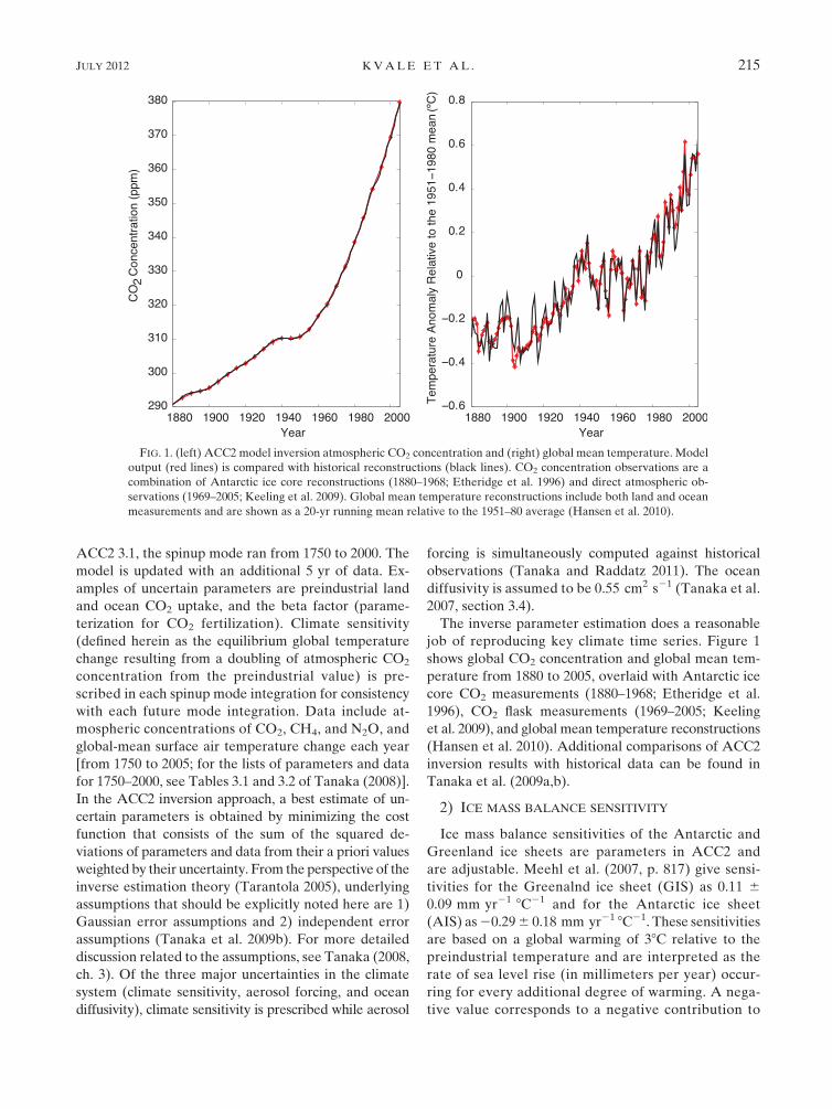
The inverse parameter estimation does a reasonable
job of reproducing key climate time series. Figure 1
shows global CO2 concentration and global mean tem-
perature from 1880 to 2005, overlaid with Antarctic ice
core CO2 measurements (1880–1968; Etheridge et al.
1996), CO2 flask measurements (1969–2005; Keeling
et al. 2009), and global mean temperature reconstructions
(Hansen et al. 2010). Additional comparisons of ACC2
inversion results with historical data can be found in
Tanaka et al. (2009a,b).
2) ICE MASS BALANCE SENSITIVITY
Ice mass balance sensitivities of the Antarctic and
Greenland ice sheets are parameters in ACC2 and
are adjustable. Meehl et al. (2007, p. 817) give sensi-
tivities for the Greenalnd ice sheet (GIS) as 0.11 60.09 mm yr21 8C21 and for the Antarctic ice sheet
(AIS) as20.296 0.18 mm yr21 8C21. These sensitivities
are based on a global warming of 38C relative to the
preindustrial temperature and are interpreted as the
rate of sea level rise (in millimeters per year) occur-
ring for every additional degree of warming. A nega-
tive value corresponds to a negative contribution to
FIG. 1. (left) ACC2 model inversion atmospheric CO2 concentration and (right) global mean temperature. Model
output (red lines) is compared with historical reconstructions (black lines). CO2 concentration observations are a
combination of Antarctic ice core reconstructions (1880–1968; Etheridge et al. 1996) and direct atmospheric ob-
servations (1969–2005; Keeling et al. 2009). Global mean temperature reconstructions include both land and ocean
measurements and are shown as a 20-yr running mean relative to the 1951–80 average (Hansen et al. 2010).
JULY 2012 KVALE ET AL . 215
sea level, or net growth of the ice sheet. Aside from
different parameter values for ice mass balance,
ACC2 treats both ice sheets identically so it is useful to
think of the combined GIS and AIS sensitivities as
a ‘‘total’’ ice sheet sensitivity. The Meehl et al. (2007,
p. 817) total sensitivity used for base runs is therefore
20.18 mm yr21 8C21.
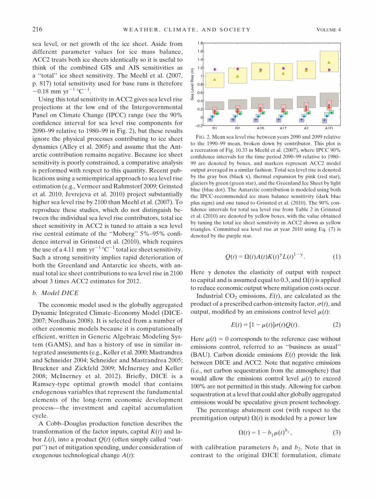
Using this total sensitivity in ACC2 gives sea level rise
projections at the low end of the Intergovernmental
Panel on Climate Change (IPCC) range (see the 90%
confidence interval for sea level rise components for
2090–99 relative to 1980–99 in Fig. 2), but these results
ignore the physical processes contributing to ice sheet
dynamics (Alley et al. 2005) and assume that the Ant-
arctic contribution remains negative. Because ice sheet
sensitivity is poorly constrained, a comparative analysis
is performed with respect to this quantity. Recent pub-
lications using a semiempirical approach to sea level rise
estimation (e.g., Vermeer andRahmstorf 2009; Grinsted
et al. 2010; Jevrejeva et al. 2010) project substantially
higher sea level rise by 2100 thanMeehl et al. (2007). To
reproduce these studies, which do not distinguish be-
tween the individual sea level rise contributors, total ice
sheet sensitivity in ACC2 is tuned to attain a sea level
rise central estimate of the ‘‘Moberg’’ 5%–95% confi-
dence interval in Grinsted et al. (2010), which requires
the use of a 4.11 mm yr21 8C21 total ice sheet sensitivity.
Such a strong sensitivity implies rapid deterioration of
both the Greenland and Antarctic ice sheets, with an-
nual total ice sheet contributions to sea level rise in 2100
about 3 times ACC2 estimates for 2012.
b. Model DICE
The economic model used is the globally aggregated
Dynamic Integrated Climate–Economy Model (DICE-
2007; Nordhaus 2008). It is selected from a number of
other economic models because it is computationally
efficient, written in Generic Algebraic Modeling Sys-
tem (GAMS), and has a history of use in similar in-
tegrated assessments (e.g., Keller et al. 2000;Mastrandrea
and Schneider 2004; Schneider and Mastrandrea 2005;
Bruckner and Zickfeld 2009; McInerney and Keller
2008; McInerney et al. 2012). Briefly, DICE is a
Ramsey-type optimal growth model that contains
endogenous variables that represent the fundamental
elements of the long-term economic development
process—the investment and capital accumulation
cycle.
A Cobb–Douglas production function describes the
transformation of the factor inputs, capital K(t) and la-
bor L(t), into a product Q(t) (often simply called ‘‘out-
put’’) net of mitigation spending, under consideration of
exogenous technological change A(t):
Q(t)5V(t)A(t)K(t)gL(t)12g . (1)
Here g denotes the elasticity of output with respect
to capital and is assumed equal to 0.3, andV(t) is applied
to reduce economic output wheremitigation costs occur.
Industrial CO2 emissions, E(t), are calculated as the
product of a prescribed carbon-intensity factor, s(t), and
output, modified by an emissions control level m(t):
E(t)5 [12m(t)]s(t)Q(t) . (2)
Here m(t) 5 0 corresponds to the reference case without
emissions control, referred to as ‘‘business as usual’’
(BAU). Carbon dioxide emissions E(t) provide the link
between DICE and ACC2. Note that negative emissions
(i.e., net carbon sequestration from the atmosphere) that
would allow the emissions control level m(t) to exceed
100% are not permitted in this study. Allowing for carbon
sequestration at a level that could alter globally aggregated
emissions would be speculative given present technology.
The percentage abatement cost (with respect to the
premitigation output) V(t) is modeled by a power law
V(t)5 12 b1m(t)b2 , (3)
with calibration parameters b1 and b2. Note that in
contrast to the original DICE formulation, climate
FIG. 2. Mean sea level rise between years 2090 and 2099 relative
to the 1990–99 mean, broken down by contributor. This plot is
a recreation of Fig. 10.33 in Meehl et al. (2007), where IPCC 90%
confidence intervals for the time period 2090–99 relative to 1980–
99 are denoted by boxes, and markers represent ACC2 model
output averaged in a similar fashion. Total sea level rise is denoted
by the gray box (black x), thermal expansion by pink (red star),
glaciers by green (green star), and the Greenland Ice Sheet by light
blue (blue dot). The Antarctic contribution is modeled using both
the IPCC-recommended ice mass balance sensitivity (dark blue
plus signs) and one tuned to Grinsted et al. (2010). The 90% con-
fidence intervals for total sea level rise from Table 2 in Grinsted
et al. (2010) are denoted by yellow boxes, with the value obtained
by tuning the total ice sheet sensitivity in ACC2 shown as yellow
triangles. Committed sea level rise at year 2010 using Eq. (7) is
denoted by the purple star.
216 WEATHER , CL IMATE , AND SOC IETY VOLUME 4
change damages are not taken into account. This implies
that cost-effective pathways do not include damage costs
to the economy, except for those associated with the
applied guardrails.2
In the original version of DICE, a globally aggregated
intertemporal social welfare functionW is maximized in
order to derive optimal climate change abatement.W is
modeled according to
W5
ðtU[C(t),L(t)](11 q)2t , (4)
U[C(t),L(t)]5L(t)[c(t)12a/(12a)] , (5)
where c(t) is per capita consumption [derived fromC(t)],
L(t) is labor, q is a social rate of time preference factor,
and a is the elasticity of the marginal utility of con-
sumption. The pure rate of social time preference is set
to 1.5% yr21, and the elasticity of the marginal utility of
consumption is set to 2 in order to achieve a real return
on capital of 5.5% yr21 over the first five decades of the
simulations (Nordhaus 2008).
Here, either 1) constrained optimal mitigation strate-
gies that obey prescribed environmental guardrails or
2) emissions corridors representing the set of all emis-
sions paths that do not violate elected environmental
guardrails and, simultaneously, a constraint on accept-
able mitigation rates are derived. In the first case (cost-
effectiveness analysis), W will be maximized subject to
the prescribed guardrails (in the absence of climate
damages, W is effectively an abatement cost function).3
In the second case (tolerable windows analysis), W is
a diagnostic variable used to compute welfare relative to
the reference case without emissions control (BAU).
Note that in contrast to traditional cost/benefit analysis
and the original formulation of Nordhaus, the welfare
function defined in this paper only takes into account
welfare losses due to mitigation measures. As long
as the pathway stays within the selected guardrails,
welfare losses due to remaining climate damages are
neglected.
c. Coupled ACC2–DICE
ACC2 contains a 255-yr spinup mode (1750–2005)
that utilizes an inversion approach to estimate uncertain
parameters and calculate starting points for the year
2005. ACC2 is run in standalone mode for the spinup
before being coupled to the mitigation cost–related
economic relationships of the DICE model for the fu-
ture runs (2005–2195). DICE operates with 10-yr time
steps, and ACC2 uses an annual iteration, so CO2
emissions from sequential iterations in DICE are lin-
early interpolated into annual values for coupling.
ACC2–DICE is run to year 2195 in order to avoid end
point effects in the time series of interest (2005–2100)
and to partially account for inertia in the climate system.
Energy-related CO2 emissions are calculated in DICE,
while CO2 emissions from land-use change and emis-
sions of non-CO2 GHGs and pollutants are prescribed
to follow IPCC SRES scenario A1B (Nakicenovic et al.
2000) until 2100. Afterward these emissions are held
constant at year 2100 levels. It is assumed that emissions
of SO2 are coupled to energy-related CO2 emissions,
considering that SO2 emissions originate mainly from
the burning of fossil fuels. A desulfurization rate of
1.5% yr21 is prescribed to account for implementation
of low-sulfur alternatives, a rate below the 2% yr21
judged to be unsustainable over the long term by
Alcamo and Kreileman (1996). Zickfeld and Bruckner
(2008) performed a sensitivity study of emissions corri-
dors with respect to the desulfurization rate and found
that reduced allowable CO2 emissions correspond with
higher desulfurization rates, owing to the faster reduction
of the aerosol cooling effect.
d. Model application schemes
1) COST-EFFECTIVENESS ANALYSIS
The objective of cost-effectiveness analysis is to cal-
culate CO2 emissions pathways that minimize abatement
costs while obeying prescribed constraints (WBGU
guardrails on global marine change, in this case). To
achieve this goal, welfare is used as the objective func-
tion. Least-cost4 emissions paths are calculated from a
start year of 2005 but constrained with WBGU guard-
rails from 2011 onward.
Note that in contrast to traditional cost/benefit
analysis, within the cost-effectiveness framework the
cost of emissions reduction and the damages caused
by climate change are not traded off. In the cost-
effectiveness framework, higher climate sensitivities
imply lower cost-effective emission trajectories. For
sufficiently high climate sensitivities, it might not be
possible to stay below the temperature limit.
2 Alternatively, the calculation presented here could be viewed
as replacing the standard DICE quasi-quadratic damage functions
with step functions that are zero within the guardrails and very high
everywhere else.3 In a strict sense, instead of minimizing pure mitigation costs,
the approach minimizes the welfare implication (losses) of miti-
gation measures.
4 ‘‘Least-cost’’ is used here in a broad sense, referring to con-
strained welfare maximization.
JULY 2012 KVALE ET AL . 217
2) TOLERABLE WINDOWS APPROACH
Cost-effectiveness analysis provides emissions path-
ways that minimize the costs of mitigation while respect-
ing climate change guardrails. From an environmental
standpoint one might rather seek to minimize climate
change subject tomitigation cost constraints. The tolerable
windows approach (Bruckner et al. 1999; Petschel-Held
et al. 1999) is a compromise between these two different
approaches as it places constraints on both environmental
impacts and mitigation costs.5 The TWA provides a
bundle of emissions paths (an ‘‘emissions corridor’’) re-
specting both climate change guardrails and an economic
constraint.
The upper (lower) bound of the emissions corridor is
calculated by maximizing (minimizing) CO2 emissions
every 10 yr, and aggregating the maxima (minima) of
the resulting paths into boundaries (Fig. 8). Stepping
outside of or even following the boundaries of the
emissions corridor violates either economic or envi-
ronmental guardrails. The converse is not necessarily
true; not all conceivable pathways within the corridor
are admissible.
Emissions corridors that comply with the WBGU
guardrails described earlier are computed here. In ad-
dition, a socioeconomic constraint is imposed to satisfy
expectations about the socioeconomically acceptable
pace of emissions reductions [see also Bruckner and
Zickfeld (2009), and references therein].
The emissions control level m(t) is not allowed to in-
crease faster than some prescribed value:
0# _m(t)# _mmax , (6)
where _mmax is set to 1.33% yr21 in this analysis. This
upper value of _mmax is based on the observed emis-
sions reductions in Germany over the 1990s (i.e., in
the years after reunification), where it is assumed
that all of the reductions are due to active mitiga-
tion in order to establish an extreme case of in-
tentional reductions (Bruckner and Zickfeld 2009).
Furthermore, in order to avoid artificial oscillations
in the emissions control level, m(t) is not allowed to
decline.
3. Results
a. Least-cost emissions paths
1) GLOBAL MEAN TEMPERATURE GUARDRAILS
The WBGU-recommended limits on global mean
temperature (28C absolute, 0.28C decade21) prove
highly constraining over the range of climate sensitivities
examined (28 to 4.58C per CO2 doubling, suggested by
the IPCC as the ‘‘likely’’ range; Meehl et al. 2007). For
climate sensitivities equal or greater than 28C, a maxi-
mum rate of temperature change of 0.28C decade21 is
not attainable because of rapid temperature increases in
the first 15 years of the twenty-first century (Fig. 3, top
middle panel). The temperature change rate guardrail is
influenced more in these early years by non-CO2 GHG
species, rendering CO2 mitigation ineffective for re-
specting temperature rate thresholds over the near term.
While the rate of temperature rise can be restrained
below the guardrail in latter decades for the higher cli-
mate sensitivities, this rate guardrail is omitted in the
rest of the analysis.
Using a 28C guardrail without a rate constraint reveals
a large dependence of the emissions pathway on the
equilibrium climate sensitivity used in the model. Figure
3 shows least-cost pathways for the 28C absolute tem-
perature change guardrail using climate sensitivities of
28, 2.58, and 38C, where a half degree of climate sensi-
tivity necessitates an additional 2–3 GtC yr21 emission
reduction by 2020, with differences increasing over the
run. For these pathways, non-CO2 GHGs and CO2
emissions from land use change are prescribed following
the IPCC SRES scenario A1B (Nakicenovic et al. 2000).
Of the climate sensitivities in the range 28 to 4.58C, only28, 2.58, and 38C produced least-cost pathways that were
able to respect the prescribed maximum temperature.
According to this analysis, should the global climate
sensitivity be greater than 38C, it would be impossible to
prevent global temperature rising beyond 28C over the
model run without emissions reduction strategies for
non-CO2 GHGs. IPCC (Meehl et al. 2007) gives a most
likely sensitivity value of about 38C, which suggests that
respecting the 28C guardrail may prove challenging if
CO2 emissions alone are mitigated. Certainly any CO2
emission pathway that does respect the WBGU global
temperature limit must depart substantially from the
DICE business-as-usual pathway within the next 5 to
10 yr (shown as a thin dotted line in Fig. 3). For a climate
sensitivity of 38C, emissions would have to be reduced by
60% (relative to BAU) by 2015 in order to respect the
absolute temperature guardrail.
The cooling role of aerosols is highlighted by the dif-
ference in the global mean temperature pathways of the
5 In a nutshell, the TWA can be described as follows: on the
basis of a set of prescribed constraints (guardrails) that exclude
intolerable climate change impacts and unacceptable mitiga-
tion measures, the admissible range of future emissions paths
is sought by investigating the dynamic relationships linking the
causes and effects of global climate change (Bruckner et al.
2003).
218 WEATHER , CL IMATE , AND SOC IETY VOLUME 4
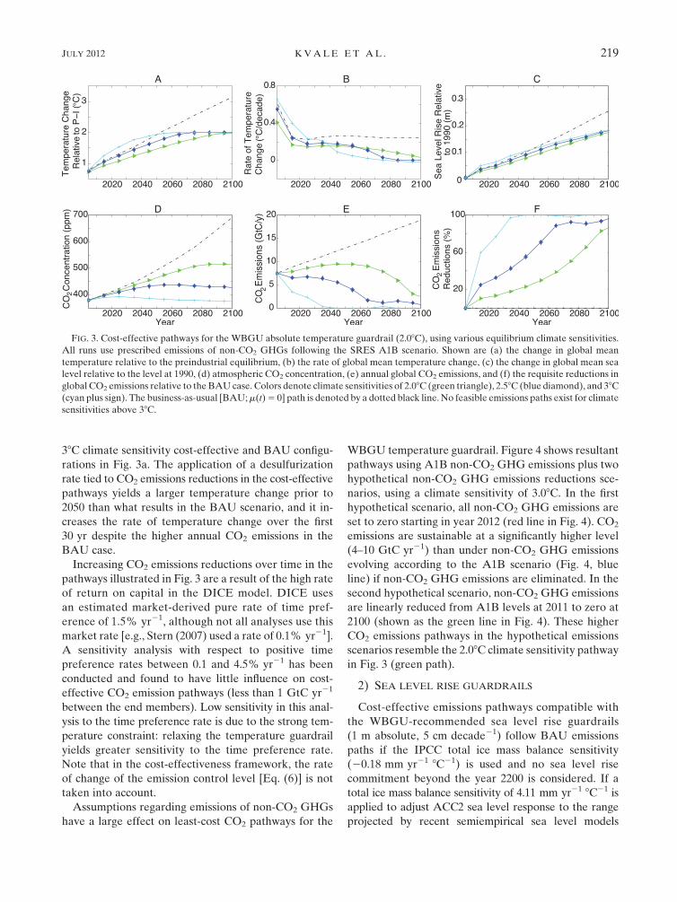
38C climate sensitivity cost-effective and BAU configu-
rations in Fig. 3a. The application of a desulfurization
rate tied to CO2 emissions reductions in the cost-effective
pathways yields a larger temperature change prior to
2050 than what results in the BAU scenario, and it in-
creases the rate of temperature change over the first
30 yr despite the higher annual CO2 emissions in the
BAU case.
Increasing CO2 emissions reductions over time in the
pathways illustrated in Fig. 3 are a result of the high rate
of return on capital in the DICE model. DICE uses
an estimated market-derived pure rate of time pref-
erence of 1.5% yr21, although not all analyses use this
market rate [e.g., Stern (2007) used a rate of 0.1% yr21].
A sensitivity analysis with respect to positive time
preference rates between 0.1 and 4.5% yr21 has been
conducted and found to have little influence on cost-
effective CO2 emission pathways (less than 1 GtC yr21
between the end members). Low sensitivity in this anal-
ysis to the time preference rate is due to the strong tem-
perature constraint: relaxing the temperature guardrail
yields greater sensitivity to the time preference rate.
Note that in the cost-effectiveness framework, the rate
of change of the emission control level [Eq. (6)] is not
taken into account.
Assumptions regarding emissions of non-CO2 GHGs
have a large effect on least-cost CO2 pathways for the
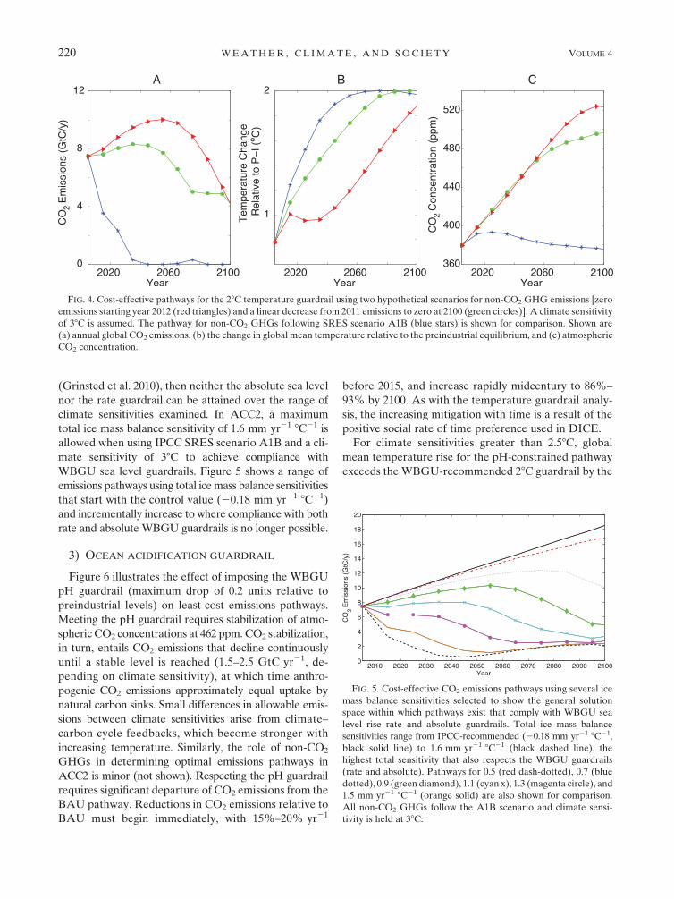
WBGU temperature guardrail. Figure 4 shows resultant
pathways using A1B non-CO2 GHG emissions plus two
hypothetical non-CO2 GHG emissions reductions sce-
narios, using a climate sensitivity of 3.08C. In the first
hypothetical scenario, all non-CO2 GHG emissions are
set to zero starting in year 2012 (red line in Fig. 4). CO2
emissions are sustainable at a significantly higher level
(4–10 GtC yr21) than under non-CO2 GHG emissions
evolving according to the A1B scenario (Fig. 4, blue
line) if non-CO2 GHG emissions are eliminated. In the
second hypothetical scenario, non-CO2 GHG emissions
are linearly reduced from A1B levels at 2011 to zero at
2100 (shown as the green line in Fig. 4). These higher
CO2 emissions pathways in the hypothetical emissions
scenarios resemble the 2.08C climate sensitivity pathway
in Fig. 3 (green path).
2) SEA LEVEL RISE GUARDRAILS
Cost-effective emissions pathways compatible with
the WBGU-recommended sea level rise guardrails
(1 m absolute, 5 cm decade21) follow BAU emissions
paths if the IPCC total ice mass balance sensitivity
(20.18 mm yr21 8C21) is used and no sea level rise
commitment beyond the year 2200 is considered. If a
total ice mass balance sensitivity of 4.11 mm yr21 8C21 is
applied to adjust ACC2 sea level response to the range
projected by recent semiempirical sea level models
FIG. 3. Cost-effective pathways for the WBGU absolute temperature guardrail (2.08C), using various equilibrium climate sensitivities.
All runs use prescribed emissions of non-CO2 GHGs following the SRES A1B scenario. Shown are (a) the change in global mean
temperature relative to the preindustrial equilibrium, (b) the rate of global mean temperature change, (c) the change in global mean sea
level relative to the level at 1990, (d) atmospheric CO2 concentration, (e) annual global CO2 emissions, and (f) the requisite reductions in
global CO2 emissions relative to theBAUcase. Colors denote climate sensitivities of 2.08C (green triangle), 2.58C (blue diamond), and 38C(cyan plus sign). The business-as-usual [BAU;m(t)5 0] path is denoted by a dotted black line. No feasible emissions paths exist for climate
sensitivities above 38C.
JULY 2012 KVALE ET AL . 219
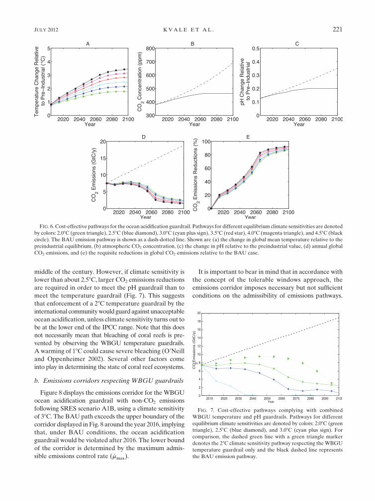
(Grinsted et al. 2010), then neither the absolute sea level
nor the rate guardrail can be attained over the range of
climate sensitivities examined. In ACC2, a maximum
total ice mass balance sensitivity of 1.6 mm yr21 8C21 is
allowed when using IPCC SRES scenario A1B and a cli-
mate sensitivity of 38C to achieve compliance with
WBGU sea level guardrails. Figure 5 shows a range of
emissions pathways using total icemass balance sensitivities
that start with the control value (20.18 mm yr21 8C21)
and incrementally increase to where compliance with both
rate and absolute WBGU guardrails is no longer possible.
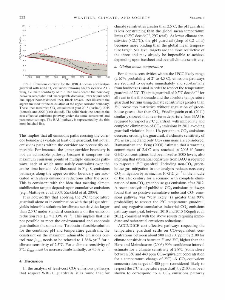
3) OCEAN ACIDIFICATION GUARDRAIL
Figure 6 illustrates the effect of imposing the WBGU
pH guardrail (maximum drop of 0.2 units relative to
preindustrial levels) on least-cost emissions pathways.
Meeting the pH guardrail requires stabilization of atmo-
sphericCO2 concentrations at 462 ppm. CO2 stabilization,
in turn, entails CO2 emissions that decline continuously
until a stable level is reached (1.5–2.5 GtC yr21, de-
pending on climate sensitivity), at which time anthro-
pogenic CO2 emissions approximately equal uptake by
natural carbon sinks. Small differences in allowable emis-
sions between climate sensitivities arise from climate–
carbon cycle feedbacks, which become stronger with
increasing temperature. Similarly, the role of non-CO2
GHGs in determining optimal emissions pathways in
ACC2 is minor (not shown). Respecting the pH guardrail
requires significant departure of CO2 emissions from the
BAU pathway. Reductions in CO2 emissions relative to
BAU must begin immediately, with 15%–20% yr21
before 2015, and increase rapidly midcentury to 86%–
93% by 2100. As with the temperature guardrail analy-
sis, the increasing mitigation with time is a result of the
positive social rate of time preference used in DICE.
For climate sensitivities greater than 2.58C, global
mean temperature rise for the pH-constrained pathway
exceeds the WBGU-recommended 28C guardrail by the
FIG. 4. Cost-effective pathways for the 28C temperature guardrail using two hypothetical scenarios for non-CO2 GHG emissions [zero
emissions starting year 2012 (red triangles) and a linear decrease from 2011 emissions to zero at 2100 (green circles)]. A climate sensitivity
of 38C is assumed. The pathway for non-CO2 GHGs following SRES scenario A1B (blue stars) is shown for comparison. Shown are
(a) annual global CO2 emissions, (b) the change in global mean temperature relative to the preindustrial equilibrium, and (c) atmospheric
CO2 concentration.
FIG. 5. Cost-effective CO2 emissions pathways using several ice
mass balance sensitivities selected to show the general solution
space within which pathways exist that comply with WBGU sea
level rise rate and absolute guardrails. Total ice mass balance
sensitivities range from IPCC-recommended (20.18 mm yr21 8C21,
black solid line) to 1.6 mm yr21 8C21 (black dashed line), the
highest total sensitivity that also respects the WBGU guardrails
(rate and absolute). Pathways for 0.5 (red dash-dotted), 0.7 (blue
dotted), 0.9 (green diamond), 1.1 (cyan x), 1.3 (magenta circle), and
1.5 mm yr21 8C21 (orange solid) are also shown for comparison.
All non-CO2 GHGs follow the A1B scenario and climate sensi-
tivity is held at 38C.
220 WEATHER , CL IMATE , AND SOC IETY VOLUME 4
middle of the century. However, if climate sensitivity is
lower than about 2.58C, larger CO2 emissions reductions
are required in order to meet the pH guardrail than to
meet the temperature guardrail (Fig. 7). This suggests
that enforcement of a 28C temperature guardrail by the
international communitywould guard against unacceptable
ocean acidification, unless climate sensitivity turns out to
be at the lower end of the IPCC range. Note that this does
not necessarily mean that bleaching of coral reefs is pre-
vented by observing the WBGU temperature guardrails.
A warming of 18C could cause severe bleaching (O’Neill
and Oppenheimer 2002). Several other factors come
into play in determining the state of coral reef ecosystems.
b. Emissions corridors respecting WBGU guardrails
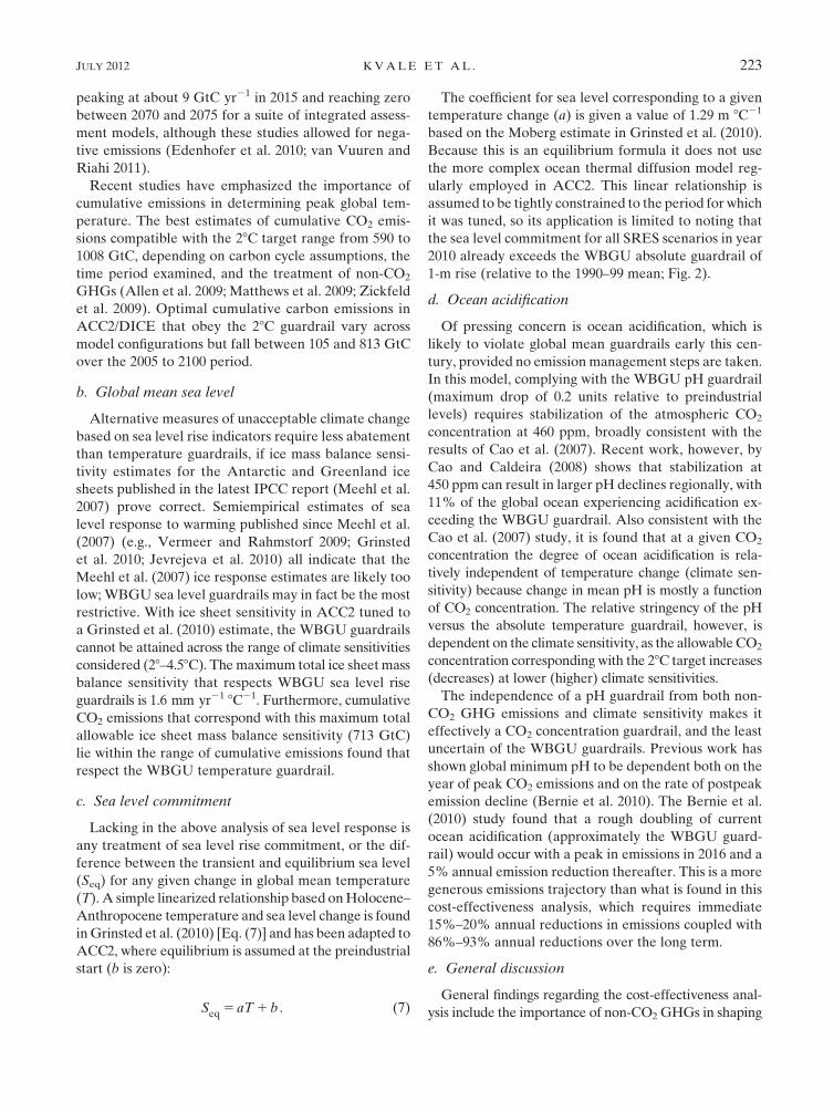
Figure 8 displays the emissions corridor for theWBGU
ocean acidification guardrail with non-CO2 emissions
following SRES scenario A1B, using a climate sensitivity
of 38C. The BAU path exceeds the upper boundary of the
corridor displayed in Fig. 8 around the year 2016, implying
that, under BAU conditions, the ocean acidification
guardrail would be violated after 2016. The lower bound
of the corridor is determined by the maximum admis-
sible emissions control rate ( _mmax).
It is important to bear in mind that in accordance with
the concept of the tolerable windows approach, the
emissions corridor imposes necessary but not sufficient
conditions on the admissibility of emissions pathways.
FIG. 6. Cost-effective pathways for the ocean acidification guardrail. Pathways for different equilibrium climate sensitivities are denoted
by colors: 2.08C (green triangle), 2.58C (blue diamond), 3.08C (cyan plus sign), 3.58C (red star), 4.08C (magenta triangle), and 4.58C (black
circle). The BAU emission pathway is shown as a dash-dotted line. Shown are (a) the change in global mean temperature relative to the
preindustrial equilibrium, (b) atmospheric CO2 concentration, (c) the change in pH relative to the preindustrial value, (d) annual global
CO2 emissions, and (e) the requisite reductions in global CO2 emissions relative to the BAU case.
FIG. 7. Cost-effective pathways complying with combined
WBGU temperature and pH guardrails. Pathways for different
equilibrium climate sensitivities are denoted by colors: 2.08C (green
triangle), 2.58C (blue diamond), and 3.08C (cyan plus sign). For
comparison, the dashed green line with a green triangle marker
denotes the 28C climate sensitivity pathway respecting the WBGU
temperature guardrail only and the black dashed line represents
the BAU emission pathway.
JULY 2012 KVALE ET AL . 221
This implies that all emissions paths crossing the corri-
dor boundaries violate at least one guardrail, but not all
emissions paths within the corridor are necessarily ad-
missible. For instance, the upper corridor boundary is
not an admissible pathway because it comprises the
maximum emissions points of multiple emissions path-
ways, each of which must satisfy constraints over the
entire time horizon. As illustrated in Fig. 8, emissions
pathways along the upper corridor boundary are asso-
ciated with steep emissions reductions after the peak.
This is consistent with the idea that meeting climate
stabilization targets depends upon cumulative emissions
(e.g., Matthews et al. 2009; Zickfeld et al. 2009).
It is noteworthy that applying the 28C temperature
guardrail alone or in combination with the pH guardrail
yields infeasible solutions for climate sensitivities larger
than 2.58C under standard constraints on the emission
reduction rate ( _m# 1:33% yr21). This implies that it is
not possible to meet the environmental and economic
guardrails at the same time. To obtain a feasible solution
for the combined pH and temperature guardrails, the
constraint on the maximum admissible emissions con-
trol rate _mmax needs to be relaxed to 1.38% yr21 for a
climate sensitivity of 2.58C. For a climate sensitivity of
38C, _mmax must be increased substantially, to 4.5% yr21.
4. Discussion
In the analysis of least-cost CO2 emissions pathways
that respect WBGU guardrails, it is found that for
climate sensitivities greater than 2.58C, the pH guardrail
is less constraining than the global mean temperature
limits (0.28C decade21, 28C total). At lower climate sen-
sitivities (,2.58C), the pH guardrail (drop of 0.2 units)
becomes more binding than the global mean tempera-
ture target. Sea level targets are the most restrictive of
the three and may already be impossible to achieve
depending upon ice sheet and overall climate sensitivity.
a. Global mean temperature
For climate sensitivities within the IPCC likely range
(a 67% probability of 28 to 4.58C), emissions pathways
are required to deviate immediately and substantially
from business as usual in order to respect the temperature
guardrail of 28C. The rate guardrail of 0.28C decade21 for
all runs in the first decade and the absolute temperature
guardrail for runs using climate sensitivities greater than
38C prove too restrictive without regulation of green-
house gases other than CO2. Friedlingstein et al. (2011)
similarly showed that near-term departure from BAU is
required to respect a 28C guardrail, with immediate and
complete elimination of CO2 emissions in 2011 avoiding
guardrail violation, but a 1% per annum CO2 emissions
decrease crossing the guardrail, if a climate sensitivity of
38C is assumed and only CO2 emissions are considered.
Ramanathan and Feng (2008) estimate that a warming
commitment of 2.48C was reached in 2005 if future
GHG concentrations had been fixed at 2005 levels, also
implying that substantial departure from BAU is required
to respect a 28C guardrail. Including non-CO2 green-
house gas mitigation in our analysis reduces necessary
CO2 mitigation by as much as 10 GtC yr21 in the middle
of the 21st century for a scenario with complete elimi-
nation of non-CO2 greenhouse gas emissions after 2012.
A recent analysis of published CO2 emissions pathways
found that no positive cumulative industrial CO2 emis-
sions pathway was ‘‘very likely’’ (a greater than 90%
probability) to respect the 28C temperature guardrail,
and any negative cumulative industrial CO2 emissions
pathway must peak between 2010 and 2015 (Rogelj et al.
2011), consistent with the above results requiring imme-
diate and substantial emissions reductions.
ACC2/DICE cost-effective pathways respecting the
temperature guardrail settle on CO2-equivalent con-
centrations between about 500 and 700 ppm by 2100 for
climate sensitivities between 28 and 38C, higher than the
Hare and Meinshausen (2006) 90% confidence interval
estimate for a climate sensitivity of 2.88C (somewhere
between 350 and 440 ppm CO2-equivalent concentration
for a temperature change of 28C). A CO2-equivalent
concentration target of 400 ppm (considered likely to
respect the 28C temperature guardrail) by 2100 has been
shown to correspond to a CO2 emissions pathway
FIG. 8. Emissions corridor for the WBGU ocean acidification
guardrail with non-CO2 emissions following SRES scenario A1B
using a climate sensitivity of 38C. Red lines denote the boundary
between acceptable and unacceptable domains (lower bound: solid
line; upper bound: dashed line). Black broken lines illustrate the
algorithm used for the calculation of the upper corridor boundary.
These lines maximize CO2 emissions in year 2015 (dashed), 2045
(dotted), and 2095 (dash-dotted). The solid black line denotes the
cost-effective emissions pathway under the same constraints and
parameter settings. The BAU pathway is represented by the thin
cross-hatched line.
222 WEATHER , CL IMATE , AND SOC IETY VOLUME 4
peaking at about 9 GtC yr21 in 2015 and reaching zero
between 2070 and 2075 for a suite of integrated assess-
ment models, although these studies allowed for nega-
tive emissions (Edenhofer et al. 2010; van Vuuren and
Riahi 2011).
Recent studies have emphasized the importance of
cumulative emissions in determining peak global tem-
perature. The best estimates of cumulative CO2 emis-
sions compatible with the 28C target range from 590 to
1008 GtC, depending on carbon cycle assumptions, the
time period examined, and the treatment of non-CO2
GHGs (Allen et al. 2009; Matthews et al. 2009; Zickfeld
et al. 2009). Optimal cumulative carbon emissions in
ACC2/DICE that obey the 28C guardrail vary across
model configurations but fall between 105 and 813 GtC
over the 2005 to 2100 period.
b. Global mean sea level
Alternative measures of unacceptable climate change
based on sea level rise indicators require less abatement
than temperature guardrails, if ice mass balance sensi-
tivity estimates for the Antarctic and Greenland ice
sheets published in the latest IPCC report (Meehl et al.
2007) prove correct. Semiempirical estimates of sea
level response to warming published since Meehl et al.
(2007) (e.g., Vermeer and Rahmstorf 2009; Grinsted
et al. 2010; Jevrejeva et al. 2010) all indicate that the
Meehl et al. (2007) ice response estimates are likely too
low; WBGU sea level guardrails may in fact be the most
restrictive. With ice sheet sensitivity in ACC2 tuned to
a Grinsted et al. (2010) estimate, the WBGU guardrails
cannot be attained across the range of climate sensitivities
considered (28–4.58C). Themaximum total ice sheetmass
balance sensitivity that respects WBGU sea level rise
guardrails is 1.6 mm yr21 8C21. Furthermore, cumulative
CO2 emissions that correspond with this maximum total
allowable ice sheet mass balance sensitivity (713 GtC)
lie within the range of cumulative emissions found that
respect the WBGU temperature guardrail.
c. Sea level commitment
Lacking in the above analysis of sea level response is
any treatment of sea level rise commitment, or the dif-
ference between the transient and equilibrium sea level
(Seq) for any given change in global mean temperature
(T). A simple linearized relationship based onHolocene–
Anthropocene temperature and sea level change is found
inGrinsted et al. (2010) [Eq. (7)] and has been adapted to
ACC2, where equilibrium is assumed at the preindustrial
start (b is zero):
Seq5 aT1 b . (7)
The coefficient for sea level corresponding to a given
temperature change (a) is given a value of 1.29 m 8C21
based on the Moberg estimate in Grinsted et al. (2010).
Because this is an equilibrium formula it does not use
the more complex ocean thermal diffusion model reg-
ularly employed in ACC2. This linear relationship is
assumed to be tightly constrained to the period for which
it was tuned, so its application is limited to noting that
the sea level commitment for all SRES scenarios in year
2010 already exceeds the WBGU absolute guardrail of
1-m rise (relative to the 1990–99 mean; Fig. 2).
d. Ocean acidification
Of pressing concern is ocean acidification, which is
likely to violate global mean guardrails early this cen-
tury, provided no emission management steps are taken.
In this model, complying with the WBGU pH guardrail
(maximum drop of 0.2 units relative to preindustrial
levels) requires stabilization of the atmospheric CO2
concentration at 460 ppm, broadly consistent with the
results of Cao et al. (2007). Recent work, however, by
Cao and Caldeira (2008) shows that stabilization at
450 ppm can result in larger pH declines regionally, with
11% of the global ocean experiencing acidification ex-
ceeding the WBGU guardrail. Also consistent with the
Cao et al. (2007) study, it is found that at a given CO2
concentration the degree of ocean acidification is rela-
tively independent of temperature change (climate sen-
sitivity) because change in mean pH is mostly a function
of CO2 concentration. The relative stringency of the pH
versus the absolute temperature guardrail, however, is
dependent on the climate sensitivity, as the allowable CO2
concentration corresponding with the 28C target increases
(decreases) at lower (higher) climate sensitivities.
The independence of a pH guardrail from both non-
CO2 GHG emissions and climate sensitivity makes it
effectively a CO2 concentration guardrail, and the least
uncertain of the WBGU guardrails. Previous work has
shown global minimum pH to be dependent both on the
year of peak CO2 emissions and on the rate of postpeak
emission decline (Bernie et al. 2010). The Bernie et al.
(2010) study found that a rough doubling of current
ocean acidification (approximately the WBGU guard-
rail) would occur with a peak in emissions in 2016 and a
5% annual emission reduction thereafter. This is a more
generous emissions trajectory than what is found in this
cost-effectiveness analysis, which requires immediate
15%–20% annual reductions in emissions coupled with
86%–93% annual reductions over the long term.
e. General discussion
General findings regarding the cost-effectiveness anal-
ysis include the importance of non-CO2 GHGs in shaping
JULY 2012 KVALE ET AL . 223
optimal emissions pathways, which suggests regulation
of a suite of GHGs to be necessary given the difficulty
already faced with meeting temperature and sea level
rate and absolute guardrails. This is corroborated by
Toth et al. (2003), Ramanathan and Feng (2008),
Zickfeld and Bruckner (2008), Gillett and Matthews
(2010), Solomon et al. (2010), and Tanaka et al. (2010),
and is particularly true should climate sensitivity prove
to be at the higher end of the IPCC range (Meehl et al.
2007). Reducing emissions of non-CO2 GHGs would
increase optimal CO2 emission pathways over the next
century, significantly so if strong reductions occur.
Declarations by the Group of Eight (G8) in recent
years for a nonbinding commitment to a 50% reduction
in global CO2 emissions (relative to some unspecified
year) by 2050 are insufficient for respecting WBGU
guardrails for any climate sensitivity above 2.58C ac-
cording to this analysis. The Stern report (Stern 2007)
concludes that CO2-equivalent concentrations should
not exceed 550 ppm if the risks of the worst climate
change impacts are to be reduced. In this modeling frame-
work, stabilizing CO2-equivalent concentration at this
level could violate all WBGU guardrails, depending upon
the climate and ice sheet mass balance sensitivities.
The emission cuts required to respect WBGU guard-
rails also respect thresholds safeguarding the stability of
the thermohaline circulation. Keller et al. (2000) found
that stabilizing CO2 concentrations between 700 to
840 ppm by 2100 would prevent a thermohaline circu-
lation collapse. CO2 concentrations admissible under the
WBGU guardrails stabilize at between 370 and 500 ppm
(roughly 500 to 700 ppm factoring in all GHGs as CO2
equivalent) in ACC2/DICE, which would maintain a
safe margin. McInerney and Keller (2008), however, point
out that the probability of crossing climate thresholds
can never be eliminated, given current parameter un-
certainty. Currently unrecognized climatic feedbacks, or
actual forcing sensitivities higher than model estimates,
could lead to unanticipated violation of WBGU guard-
rails. Furthermore, welfare or abatement optimizing
methods may give less robust mitigation strategies with
respect to avoiding dangerous climate thresholds than
those that balance uncertainty against worst-case losses
in utility (McInerney et al. 2012).
f. Tolerable emissions corridors
The tolerable windows approach addresses a criticism
of cost-effectiveness analysis in that instead of providing
one stringent pathway that might be difficult to follow
precisely or difficult to negotiate, it calculates a tolerable
emissions corridor. This analysis of the WBGU guard-
rail for temperature suggests that attaining both eco-
nomic and environmental guardrails is feasible only for
climate sensitivities #2.58C, if non-CO2 GHGs are not
also mitigated. This infeasible result for the temperature
guardrail using higher climate sensitivities highlights the
quickly diminishing options. Earlier work by Kriegler
and Bruckner (2004) examined a 28C temperature guard-
rail for a climate sensitivity of 3.58C using similar methods
and found a feasible corridor peaking at 10 GtC yr21.
Emissions corridors complying with the pH guardrail
alone are feasible solutions in this analysis. These cor-
ridors would simultaneously safeguard against thermo-
haline circulation collapse, which requires the upper
corridor bound to peak between 20 and 90 GtC yr21
(depending on the value of hydrological sensitivity) for a
3.58C climate sensitivity (Zickfeld and Bruckner 2008).
g. Sensitivity of economic parameters
There are several contentious assumptions and pa-
rameters within the DICE model, most notably the
market-derived social rate of time preference factor (q)
[see discussions in Nordhaus (2008) and Stern (2007)]. A
sensitivity study is conducted with regard to both the
social rate of time preference and abatement cost func-
tion parameters in the DICE model, and cost-effective
CO2 emissions pathways are found to be insensitive
(less than 1 GtC yr21) to parameter choice owing to the
dominance of the temperature and pH guardrails in
determining optimal pathways and corridors. Emissions
corridors, however, are sensitive to the mitigation con-
straint ( _mmax # 1:33% yr21). Relaxing the constraint on
the maximum rate of emissions reductions affects only
the lower corridor boundary, consistent with the results of
Bruckner and Zickfeld (2009). Tolerable maximum
levels of mitigation are, however, open political questions
and this analysis foreshadows a looming choice between
respecting either tolerable economic or tolerable climate
guardrails.
5. Conclusions
Given commonly assumed central estimates of cli-
mate sensitivity, and an ice sheet sensitivity estimate
derived from past ice sheet changes, the rate threshold
for temperature (0.28C decade21) and the absolute
and rate thresholds for sea level rise (1 m absolute,
5 cm decade21) are not attainable in this simulation
framework. Limiting absolute temperature change to
28C is still an achievable target should climate sensitivity
be 38C or less, but immediate and drastic mitigative ac-
tion is required, which might violate assumed tolerable
decarbonization rates. Emissions reductions required
to limit changes in surface ocean pH to less than 0.2 units
globally are less stringent, provided emissions reduc-
tions start now. These results indicate that because of
224 WEATHER , CL IMATE , AND SOC IETY VOLUME 4
global inaction on climate change, achievement of cli-
mate targets avoiding dangerous ocean impacts has be-
come very difficult, and in some cases impossible.
This analysis addresses mitigation of CO2 emissions
only. Neglecting non-CO2 mitigation biases results in
unrealistic high/fast CO2 emissions reduction. Mitigat-
ing emissions of other non-CO2 GHGs would increase
the leeway for action and could have a large influence
on the attainability of the temperature guardrails in par-
ticular. In the case of sea level rise, the current primary
uncertainty in allowable emissions is the sensitivity of
ice sheets to warming. Emissions complying with ocean
acidification guardrails are the least uncertain of those
examined as they are independent of both climate sensi-
tivity and non-CO2 GHG emissions. Emissions pathways
obeying the temperature and sea level rise guardrails are
influenced by the relatively short time horizon of the
analysis owing to the thermal inertia of the earth system.
Allowable twenty-first-century emissions would likely
be lower if the long-term climate commitment was
considered.
Acknowledgments. The authors thank Ed Wiebe and
Michael Eby for technical support. KJM is grateful for
research grant support under the University Faculty
Award program and the Discovery Program from the
Natural Sciences and Engineering Research Council
of Canada (NSERC). We are grateful for funding sup-
port from NSERC and the Canadian Foundation for
Climate and Atmospheric Sciences. K. Tanaka is partly
supported by the Marie Curie Intra-European Fellow-
ship within the 7th European Community Framework
Programme (Proposal N255568 under FP7-PEOPLE-
2009-IEF).
APPENDIX
Additional ACC2 Model Description
a. Computation of pH
Global mean pH and the thermodynamic equilibria of
marine carbonate species [CO2(aq), HCO23 , and CO22
3 ]
are computed in ACC2 to model the saturation effect in
ocean CO2 uptake under rising CO2 concentration. A
more detailed description can be found in Tanaka (2008,
sections 2.1.2 and 2.1.4). The following chemical re-
actions govern the marine carbonate system:
CO2(g) 4 CO2(aq), (A1)
CO2(aq)1H2O 4 H11HCO23 , (A2)
HCO23 4 H11CO22
3 , (A3)
H2O 4 H11OH2 , (A4)
B(OH)24 1H1 4 B(OH)31H2O. (A5)
These equations represent the dissolution and hy-
dration of carbon dioxide [Eq. (A1)], the dissociation of
carbon dioxide into bicarbonate, hydrogen, and carbonate
[Eqs. (A2) and (A3)], the self-dissociation of water [Eq.
(A4)], and the dissociation of borate [Eq. (A5)].
Characterization of the carbonate system requires
the estimates of two of the following four measurable
quantities: pH, total alkalinity ([TA]), dissolved in-
organic carbon ([DIC]), and the CO2 partial pressure
(pCO2) (Park 1969; Millero 2006). These quantities
are defined as follows:
pH52log10([H1]) , (A6)
[TA]5 2[CO223 ]1 [HCO2
3 ]1 [B(OH)24 ]
1 [OH2]2 [H1] , (A7)
[DIC]5 [CO223 ]1 [HCO2
3 ]1 [CO2(aq)] , (A8)
pCO251
K0*[CO2(aq)] . (A9)
In Eq. (A9), K0* is the inverse of Henry’s constant. A
constant value for [TA] is assumed because a significant
amount of carbonate precipitation or dissolution or
addition of alkalinity from land did not occur during the
historical period of the model run (Mackenzie and
Lerman 2006) and is assumed negligible for the next
hundreds of years. Also, pCO2 is given in each time
step in the model. The remaining two variables pH and
[DIC] are determined by solving the following two
equations:
[TA]5 pCO2K0*
11
K1*
[H1]1
K1*K2*
[H1]2
!
1[B(OH)24 ]1 [B(OH)3]
11[H1]
KB*
1Kw*
[H1]2 [H1] ,
(A10)
[DIC]5 pCO2K0*
11
K1*
[H1]1
K1*K2*
[H1]2
!. (A11)
Here K1*, K2*, Kw*, and KB* are the thermodynamic
equilibrium constants associated with Eqs. (A2)–(A5),
respectively. These constants are given as a function of
mixed-layer temperature (Millero 1995; Millero et al.
2006).
JULY 2012 KVALE ET AL . 225
b. Sea level calculation
Global sea level rise in ACC2 is calculated following
expressions given in the Third Assessment Report (TAR)
of the IPCC (Houghton et al. 2001, appendix 11.1),
where it is a sum of contributions from mass loss from
the Greenland and Antarctic ice sheets in response to
ongoing and past climate change, thermal expansion, the
loss of mass from glaciers and small ice caps, runoff from
thawing permafrost, and sediment deposition on the sea
floor. Contributions from the AIS, GIS, permafrost,
thermal expansion, and sediment deposition are parame-
terized as functions of global mean temperature. The
contribution of glaciers and small ice caps (g) is calcu-
lated as
g(t)5 0:934gu(t)2 1:165g2u(t) , (A12)
where gu is the loss of mass with respect to the glacier
steady state without consideration of area contraction
and is derived from an integration of global temperature
with respect to time. This is an empirical relationship
taken from a quadratic fit to the atmosphere–ocean
GCM (AOGCM) scenario IS92a (Houghton et al. 2001,
ch. 11). This relationship holds until around 2160,
whereupon the second term grows larger than the first
and glaciers and small ice caps show net growth, an
unphysical result.
Two modifications are made to the sea level calcula-
tion in ACC2 for the purposes of this study. To avoid the
unphysical result of growing glacier and small ice caps
after 2160, a smoothing function is implemented after a
critical level of sea level rise (gcritical, with a corre-
sponding temperatureTcritical) where contribution to sea
level rise from glaciers and small ice caps follows an
exponential curve to a prescribed maximum. This
smoothing function is described in Eq. (A13), where
gsmooth is the difference between the prescribed maxi-
mum sea level rise and gcritical, and Sinit is the slope of the
function immediately before gcritical:
g(T)5 gcritical 1 gsmooth[12 e[sinit /(2gsmooth
)](T2Tcritical
)] .
(A13)
Meehl et al. (2007) estimate the total potential sea level
contribution fromglaciers and small ice caps to be between
0.15 and 0.37 m. The values of gcritical (0.28 m relative to
preindustrial equilibrium, of which 0.03 m had already
occurred by 2000 in ACC2) and gsmooth (0.07 m) are
selected based on these estimates, so that total glacial
contribution does not exceed 0.35 m for any scenario. In
this new method, Eq. (A12) calculates glacier contri-
bution to sea level rise up until the gcritical value is
reached, whereupon it is replaced by Eq. (A13). Having
a continuous sea level contribution for glaciers and small
ice caps is critical for setting a guardrail in DICE.
Second the calculation of thermal expansion is modi-
fied from one based on surface temperature to one
derived from the thermal anomaly throughout the water
column as calculated by the energy balance model
DOECLIM. The parameterization in Houghton et al.
(2001, appendix 11.1) is used, where sea level rise due to
thermal expansion is relative to that in year 1990. To
calculate thermal expansion explicitly, the interior ocean
temperature is first found as a function of depth and time
(T0). Using a pure diffusion model without upwelling,
where heat diffusion is described as follows,
for 0, z, zB :›
›tTo(z, t)5 ky
›2
›z2To(z, t) , (A14)
B.C: : To(0, t)5Ts(t),›
›zTo(zB, t)5 0, (A15)
I.C. :To(z, 0)5 0: (A16)
In this case, the upper boundary (z 5 0) to the mixed
layer has the same temperature as the mixed layer Ts,
and the heat flux into the ocean floor at z5 zB vanishes.
The solution for To is solved analytically by Kriegler
(2005, appendix B):
To(z, t)5Ts(t)2
ðt0
_Ts(t9) Erf
"z
2ffiffiffiffiffiffiffiffiffiffiffiffiffiffiffiffiffiffiffiky(t2 t9)
p#dt91 �
1‘
n51
(21)nðt0
_Ts(t9)
(Erf
"2nzB 2 z
2ffiffiffiffiffiffiffiffiffiffiffiffiffiffiffiffiffiffiffiffiffiky(t 2 t9)
p#2Erf
"2nzB 1 z
2ffiffiffiffiffiffiffiffiffiffiffiffiffiffiffiffiffiffiffiffiffiky(t 2 t9)
p#)
dt9 ,
(A17)
where Ts is ocean surface temperature, z is ocean depth,
ky is the vertical diffusivity with a value of 0.55 cm2 s21, n
is a bottom correction term, and Erf is the error function.
The series in Eq. (A17) converges quickly, so the only
terms of importance are that of the zeroth-order term
describing the behavior of an infinitely deep ocean and
one to three next-order bottom correction terms. Inclu-
sion of the bottom correction terms in Eq. (A17) is not
necessary for the length of time the model is run as it
makes only a small difference in the thermal profile
(roughly 9 mm by 2200). Once the thermal profile is cal-
culated, To is plugged in to the linearized equation of state:
226 WEATHER , CL IMATE , AND SOC IETY VOLUME 4
r(z, t) 5 r0(z)f1 2 a[To(z, t) 2 T0(z)]
1b[S(z, t) 2 S0(z)]g . (A18)
In Eq. (A18), r is density, a is a coefficient of thermal
expansion (1.7 exp24 K21), b is the coefficient of saline
contraction, and S is salinity. Constant salinity is as-
sumed for simplification, and the last term drops out.
Rearranging Eq. (A18) to isolate both r terms on one
side gives a ratio of change for each time step in each
depth. Multiplying this ratio by the layer thickness at
each depth and summing over z yields the thermal ex-
pansion in meters.
This explicit calculation adds the capability of track-
ing the evolution of interior ocean temperature and
density profiles, an improvement over the impulse re-
sponse approach. The estimate of thermal expansion pro-
duced using the updated equation is lower than
that produced by the impulse response function while still
being within the range estimated by Meehl et al. (2007).
REFERENCES
Alcamo, J., and E. Kreileman, 1996: Emission scenarios and
global climate protection. Global Environ. Change, 6, 305–334, doi:10.1016/S0959-3780(96)00030-1.
Allen, M. R., D. J. Frame, C. Huntingford, C. D. Jones, J. A. Lowe,
M. Meinshausen, and N. Meinshausen, 2009: Warming caused
by cumulative carbon emissions towards the trillionth tonne.
Nature, 458, 1163–1166.
Alley, R., P. Clark, P. Huybrechts, and I. Joughin, 2005: Ice-sheet
and sea-level changes. Science, 310, 456–460, doi:10.1126/
science.1114613.
Bali Declaration, 2007: 2007 Bali Climate Declaration by Scien-
tists. [Available online at http://www.ccrc.unsw.edu.au/news/
2007/Bali.html.]
Barnett, J., and W. Adger, 2003: Climate dangers and atoll coun-
tries. Climatic Change, 61, 321–337.
Bernie, D., J. Lowe, T. Tyrrell, and O. Legge, 2010: Influence of
mitigation policy on ocean acidification. Geophys. Res. Lett.,
37, L15704, doi:10.1029/2010GL043181.
Bruckner, T., and K. Zickfeld, 2009: Emissions corridors for re-
ducing the risk of a collapse of the Atlantic thermohaline
circulation. Mitigation Adapt. Strategies Global Change, 14,61–83.
——,G. Petschel-Held, F. Toth,H.-M. Fussel, C.Helm,M. Leimbach,
and H.-J. Schellnhuber, 1999: Climate change decision-
support and the tolerable windows approach.Environ.Model.
Assess., 4, 217–234.
——, ——, M. Leimbach, and F. Toth, 2003: Methodological as-
pects of the tolerable windows approach. Climatic Change, 56,73–89.
Buddemeier, R. W., J. A. Kleypas, and R. B. Aronson, 2004: Coral
reefs and global climate change: Potential contributions of
climate change to stresses on coral reef ecosystems. Pew
Center on Global Climate Change, 44 pp.
Cao, L., and K. Caldeira, 2008: Atmospheric CO2 stabilization
and ocean acidification. Geophys. Res. Lett., 35, L19609,
doi:10.1029/2008GL035072.
——, ——, and A. K. Jain, 2007: Effects of carbon dioxide and
climate change on ocean acidification and carbonate min-
eral saturation. Geophys. Res. Lett., 34, L05607, doi:10.1029/
2006GL028605.
Copenhagen Accord, 2009: Copenhagen Accord. [Available
online at http://unfccc.int/resource/docs/2009/cop15/eng/11a01.
pdf.]
Corfee-Morlot, J., andN.Hohne, 2003: Climate change: Long-term
targets and short-term commitments. Global Environ. Change,
13, 277–293, doi:10.1016/j.gloenvcha.2003.09.001.
Dessai, S., W. Adger, M. Hulme, J. Turnpenny, J. Kohler,
and R. Warren, 2004: Defining and experiencing dangerous
climate change: An editorial essay. Climatic Change, 64,
11–25.
ECF, 2004: What is dangerous climate change? Initial results of
a symposium on key vulnerable regions: Climate change and
article 2 of the UNFCCC. [Available online at http://www.
globalclimateforum.org/fileadmin/ecf-documents/publications/
articles-and-papers/what-is-dangerous-climate-change.pdf.]
Edenhofer, O., and Coauthors, 2010: The economics of low stabi-
lization: Model comparison of mitigation strategies and costs.
Energy J., 31, 11–48.
Etheridge, D., L. Steele, R. Langenfelds, R. Francey, J. Barnola,
and V. Morgan, 1996: Natural and anthropogenic changes
in atmospheric CO2 over the last 1000 years from air in
Antarctic ice and firn. J. Geophys. Res., 101, 4115–4128.Fischlin, A., and Coauthors, 2007: Ecosystems, their properties,
goods and services.Climate Change 2007: Impacts, Adaptation
and Vulnerability, M. L. Parry et al., Eds., Cambridge Uni-
versity Press, 211–272.
Friedlingstein, P., S. Solomon, G.-K. Plattner, R. Knutti, P. Ciais,
and M. R. Raupach, 2011: Long-term climate implications
of twenty-first century options for carbon dioxide emission
mitigation. Nature Climate Change, 1, 457–461, doi:10.1038/nclimate1302.
Funk, C., M. D. Dettinger, J. C. Michaelsen, J. P. Verdin, M. E.
Brown,M. Barlow, andA. Hoell, 2008:Warming of the Indian
Ocean threatens eastern and southern African food security
but could be mitigated by agricultural development. Proc.
Natl. Acad. Sci. USA, 105, 11 081–11 086, doi:10.1073/pnas.
0708196105.
Gillett, N. P., and H. D. Matthews, 2010: Accounting for carbon
cycle feedbacks in a comparison of the global warming effects
of greenhouse gases. Environ. Res. Lett., 5, 034011, doi:10.1088/
1748-9326/5/3/034011.
Graßl, H., and Coauthors, 2003: Climate protection strategies for
the 21st century: Kyoto and beyond. German Advisory
Council on Global Change, 77 pp. [Available online at http://
www.wbgu.de/en/special-reports/sr-2003-kyoto-and-beyond/.]
Greenpeace, 2008: Greenpeace demands at G8: Real action on
climate change and food crisis, business as usual is not an option.
[Available online at http://www.greenpeace.org/international/
press/releases/greenpeace-demands-at-g8.]
Grinsted, A., J. C. Moore, and S. Jevrejeva, 2010: Reconstructing
sea level from paleo and projected temperatures 200 to 2100
AD. Climate Dyn., 34, 461–472, doi:10.1007/s00382-008-
0507-2.
Hansen, J., 2005: A slippery slope: How much global warming
constitutes ‘‘dangerous anthropogenic interference’’? Climatic
Change, 68, 269–279.——, R. Ruedy, M. Sato, and K. Lo, 2010: Global surface tem-
perature change. Rev. Geophys., 48, RG4004, doi:10.1029/
2010RG000345.
JULY 2012 KVALE ET AL . 227
Hare, B., and M. Meinshausen, 2006: How much warming are
we committed to and how much can be avoided? Climatic
Change, 75, 111–149, doi:10.1007/s10584-005-9027-9.
Harvey, L. D. D., 2007: Allowable CO2 concentrations under the
United Nations Framework Convention on Climate Change
as a function of the climate sensitivity probability distribution
function.Environ. Res. Lett., 2, 014001, doi:10.1088/1748-9326/
2/1/014001.
Hooss, G., R. Voss, K. Hasselmann, E. Maier-Reimer, and F. Joos,
2001: A nonlinear impulse response model of the coupled
carbon cycle–climate system (NICCS). Climate Dyn., 18, 189–
202.
Houghton, J., Y. Ding, D. Griggs, M. Noguer, P. van der Linden,
X. Dai, K. Maskell, and C. Johnson, 2001: Climate Change
2001: The Scientific Basis. Cambridge University Press, 881 pp.
Jevrejeva, S., J. C.Moore, andA.Grinsted, 2010:Howwill sea level
respond to changes in natural and anthropogenic forcings
by 2100? Geophys. Res. Lett., 37, L07703, doi:10.1029/
2010GL042947.
Joos, F., M. Bruno, R. Fink, U. Siegenthaler, and T. Stocker, 1996:
An efficient and accurate representation of complex oceanic
and biospheric models of anthropogenic carbon uptake.
Tellus, 48B, 397–417.——, I. Prentice, S. Sitch, R. Meyer, G. Hooss, G. Plattner,
S. Gerber, and K. Hasselmann, 2001: Global warming feed-
backs on terrestrial carbon uptake under the Intergovern-
mental Panel on Climate Change (IPCC) emission scenarios.
Global Biogeochem. Cycles, 15, 891–907.
Keeling, C. D., S. C. Piper, A. F. Bollenbacher, and J. S. Walker,
cited 2009: Atmospheric CO2 records from sites in the SIO air
sampling network. [Available online at http://cdiac.ornl.gov/
trends/co2/sio-keel.html.]
Keller, K., K. Tan, F. Morel, and D. Bradford, 2000: Preserving the
ocean circulation: Implications for climate policy. Climatic
Change, 47, 17–43.
——, M. Hall, S. Kim, D. Bradford, and M. Oppenheimer, 2005:
Avoiding dangerous anthropogenic interference with the cli-
mate system. Climatic Change, 73, 227–238.
Kriegler, E., 2005: Imprecise probability analysis for integrated
assessment of climate change. Ph.D. thesis, University of
Potsdam, 258 pp.
——, and T. Bruckner, 2004: Sensitivity analysis of emissions cor-
ridors for the 21st century. Climatic Change, 66, 345–387.
Lenton, T. M., and Coauthors, 2007: Effects of atmospheric dy-
namics and ocean resolution on bi-stability of the thermoha-
line circulation examined using the Grid Enabled Integrated
Earth system modelling (GENIE) framework. Climate Dyn.,
29, 591–613, doi:10.1007/s00382-007-0254-9.
Mackenzie, F., and A. Lerman, 2006: Carbon in the Geobiosphere:
Earth’s Outer Shell. Springer, 402 pp.
Mastrandrea, M., and S. Schneider, 2004: Probabilistic integrated
assessment of ‘‘dangerous’’ climate change. Science, 304, 571–575.
Matthews, H. D., N. P. Gillett, P. A. Stott, and K. Zickfeld, 2009:
The proportionality of global warming to cumulative carbon
emissions. Nature, 459, 829–832.McInerney, D., and K. Keller, 2008: Economically optimal risk
reduction strategies in the face of uncertain climate thresh-
olds. Climatic Change, 91, 29–41, doi:10.1007/s10584-006-
9137-z.
——, R. Lempert, and K. Keller, 2012: What are robust strategies
in the face of uncertain climate threshold responses? Climatic
Change, 112, 547–568, doi:10.1007/s10584-011-0377-1.
Meehl, G., and Coauthors, 2007: Global climate projections. Cli-
mate Change 2007: The Physical Science Basis, S. Solomon
et al., Eds., Cambridge University Press, 747–845.
Millero, F., 1995: Thermodynamics of the carbon-dioxide system in
the oceans. Geochim. Cosmochim. Acta, 59, 661–677.
——, 2006: Chemical Oceanography. 3rd ed. CRC Press, 496 pp.
——, T. Graham, F. Huang, H. Bustos-Serrano, and D. Pierrot,
2006: Dissociation constants of carbonic acid in seawater as
a function of salinity and temperature.Marine Chem., 100, 80–
94, doi:10.1016/j.marchem.2005.12.001.
Nakicenovic, N., and Coauthors, 2000: Special Report on Emissions
Scenarios. Cambridge University Press, 599 pp.
Nicholls, R., P. P. Wong, V. Burkett, J. Codignotto, J. Hay,
R. McLean, S. Ragoonaden, and C. Woodroffe, 2007: Coastal
systems and low-lying areas. Climate Change 2007: Climate
Change Impacts, Adaptation and Vulnerability. M. L. Parry
et al., Eds., Cambridge University Press, 315–356.
Nordhaus, W., 1992: An optimal transition path for controlling
greenhouse gases. Science, 258, 1315–1319.——, 1994: Managing the Global Commons: The Economics of
Climate Change. MIT Press, 213 pp.
——, 2008:AQuestion of Balance:Weighing theOptions onGlobal
Warming Policies. Yale University Press, 234 pp.
——, and J. Boyer, 2000:Warming the World: Economic Models of
Global Warming. MIT Press, 244 pp.
O’Neill, B., and M. Oppenheimer, 2002: Dangerous climate im-
pacts and the Kyoto protocol. Science, 296, 1971–1972.
Oppenheimer, M., and R. Alley, 2004: The West Antarctic ice
sheet and long term climate policy: An editorial comment.
Climatic Change, 64, 1–10.Orr, J., and Coauthors, 2005: Anthropogenic ocean acidification
over the twenty-first century and its impact on calcifying or-
ganisms. Nature, 437, 681–686, doi:10.1038/nature04095.
Park, K., 1969: Oceanic CO2 system: An evaluation of ten methods
of investigation. Limnol. Oceanogr., 14, 179–186.
Parry, M., and Coauthors, 2001: Millions at risk: Defining critical
climate change threats and targets. Global Environ. Change,
11, 181–183.
Pauly, D., R. Watson, and J. Alder, 2005: Global trends in world
fisheries: Impacts on marine ecosystems and food security.
Philos. Trans. Roy. Soc., 360B, 5–12, doi:10.1098/rstb.
2004.1574.
Petschel-Held, G., H. Schellnhuber, T. Bruckner, F. Toth, and
K. Hasselmann, 1999: The tolerable windows approach: The-
oretical andmethodological foundations.Climatic Change, 41,303–331.
Ramanathan, V., and Y. Feng, 2008: On avoiding dangerous an-
thropogenic interference with the climate system: Formidable
challenges ahead. Proc. Natl. Acad. Sci. USA, 105, 14 245–
14 250, doi:10.1073/pnas.0803838105.
Rogelj, J., and Coauthors, 2011: Emission pathways consistent with
a 28Cglobal temperature limit.Nature Climate Change, 1, 413–418, doi:10.1038/nclimate1258.
Schneider, S., and M. Mastrandrea, 2005: Probabilistic assessment
‘‘dangerous’’ climate change and emissions pathways. Proc.
Natl. Acad. Sci. USA, 102, 15 728–15 735, doi:10.1073/pnas.
0506356102.
——, and Coauthors, 2007: Assessing key vulnerabilities and the
risk from climate change. Climate Change 2007: Impacts,
Adaptation and Vulnerability. M. L. Parry et al., Eds., Cam-
bridge University Press, 779–810.
Schubert, R., and Coauthors, 2006: The future oceans: Warming
up, rising high, turning sour. German Advisory Council on
228 WEATHER , CL IMATE , AND SOC IETY VOLUME 4
Global Change, 110 pp. [Available online at http://cmbc.ucsd.
edu/Research/Climate_Change/Future%20Oceans.pdf.]
Smith, J., and Coauthors, 2001: Vulnerability to climate change
and reasons for concern: A synthesis. Climate Change 2001:
Impacts, Adaptation and Vulnerability, J. J. McCarthy et al.,
Eds., Cambridge University Press, 913–967.
Solomon, S., J. S. Daniel, T. J. Sanford, D. M. Murphy, G.-K.
Plattner, R. Knutti, and P. Friedlingstein, 2010: Persistence of
climate changes due to a range of greenhouse gases. Proc. Natl.
Acad. Sci. USA, 107, 18 354–18 359, doi:10.1073/pnas.1006282107.
Stern, N., 2007: The Economics of Climate Change. Cambridge
University Press, 692 pp.
Tanaka, K., 2008: Inverse estimation for the simple earth system
model ACC2 and its applications. Ph.D. thesis, Hamburg
University, International Max Planck Research School on
Earth System Modelling, 296 pp. [Available online at http://
www.sub.uni-hamburg.de/opus/volltexte/2008/3654.]
——, and T. Raddatz, 2011: Correlation between climate sensitivity
and aerosol forcing and its implication for the ‘‘climate trap.’’
Climatic Change, 109, 815–825, doi:10.1007/s10584-011-0323-2.
——, E. Kriegler, T. Bruckner, G. Hooss, W. Knorr, and T. Raddatz,
2007: Aggregated carbon cycle, atmospheric chemistry, and cli-
mate model (ACC2): Description of the forward and inverse
modes. Reports on Earth System Science No. 40, Max Planck
Institute for Meteorology, 188 pp.
——, B. O’Neill, D. Rokityanskiy, M. Obersteiner, and R. Tol,
2009a: Evaluating global warming potentials with historical
temperature. Climatic Change, 96, 443–466.
——, T. Raddatz, B. O’Neill, and C. Reick, 2009b: Insufficient
forcing uncertainty underestimates the risk of high climate
sensitivity. Geophys. Res. Lett., 36, L16709, doi:10.1029/
2009GL039642.
——, G. Peters, and J. Fuglestvedt, 2010: Multicomponent climate
policy: Why do emission metrics matter? Carbon Manage., 1,191–197.
Tarantola, A., 2005: Inverse Problem Theory and Methods for
Model Parameter Estimation. Society for Industrial and Ap-
plied Mathematics, 342 pp.
Toth, F., T. Bruckner,H. Fussel,M. Leimbach, andG. Petschel-Held,
2003: Integrated assessment of long-term climate policies. Part
2: Model results and uncertainty analysis. Climatic Change, 56,
57–72.
UNFCCC, 1992:UnitedNations FrameworkConvention onClimate
Change. [Available online at http://unfccc.int/key_documents/
the_convention/items/2853.php.]
Union of Concerned Scientists, 2007: A target for U.S. emissions
reductions. [Available online at http://www.ucsusa.org/global_
warming/solutions/big_picture_solutions/a-target-for-us-emissions.
html.]
van Vuuren, D. P., and K. Riahi, 2011: The relationship between
short-term emissions and long-term concentration targets.
Climatic Change, 104, 793–801, doi:10.1007/s10584-010-
0004-6.
Vermeer, M., and S. Rahmstorf, 2009: Global sea level linked to
global temperature. Proc. Natl. Acad. Sci. USA, 106, 21 527–
21 532, doi:10.1073/pnas.0907765106.
Zeebe, R. E., J. C. Zachos, K. Caldeira, and T. Tyrrell, 2008:
Carbon emissions and acidification. Science, 321, 51–52,
doi:10.1126/science.1159124.
Zickfeld, K., and T. Bruckner, 2003: Reducing the risk of abrupt
climate change: Emissions corridors preserving the Atlantic
thermohaline circulation. Integr. Assess., 4, 106–115.
——, and——, 2008: Reducing the risk of Atlantic thermohaline
circulation collapse: Sensitivity analysis of emissions corri-
dors. Climatic Change, 91, 291–315, doi:10.1007/s10584-008-9467-0.
——, M. Eby, H. Matthews, and A. Weaver, 2009: Setting cu-
mulative emissions targets to reduce the risk of dangerous
climate change. Proc. Natl. Acad. Sci. USA, 106, 16 129–
16 134, doi:10.1073/pnas.0805800106.
JULY 2012 KVALE ET AL . 229