12/2/2014

1

Risk and Uncertainty

Overview This chapter deals with the role of risk and uncertainty in an economy. Buying stocks is an example of this scenario, where there is a potential payoff, but also a potential risk of losing money.  

We will analyze how to describe these situations, and how to predict how a decision‐maker will act in the face of risk. 

Lottery A lottery is simply any event in which the outcome is uncertain, much like our example about investing in stocks or the outcome of a college football game

Probability is the likelihood that a specific outcome will occur (e.g. ,the likelihood of earning a positive return on the stock you purchased)

We can illustrate a lottery in the form of a chart…

Furthermore, the probability distribution is a graph that depicts all possible outcomes and their associated probabilities, as depicted below.

30%

40%

30%

12/2/2014

2

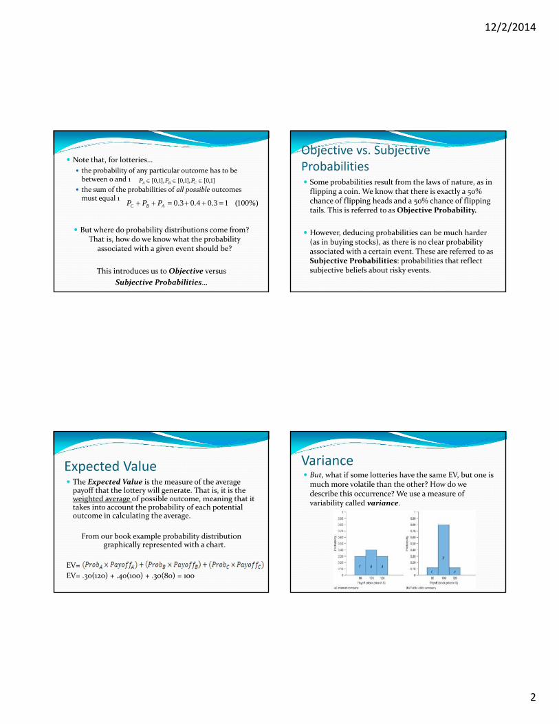
Note that, for lotteries…

the probability of any particular outcome has to be between 0 and 1

the sum of the probabilities of all possible outcomes must equal 1

But where do probability distributions come from?  That is, how do we know what the probability 

associated with a given event should be?

This introduces us to Objective versus 

Subjective Probabilities…

PA [0,1],PB [0,1],PC [0,1]

PC PB PA 0.3 0.4 0.3 1 (100%)

Objective vs. Subjective Probabilities Some probabilities result from the laws of nature, as in flipping a coin. We know that there is exactly a 50% chance of flipping heads and a 50% chance of flipping tails. This is referred to as Objective Probability. 

However, deducing probabilities can be much harder (as in buying stocks), as there is no clear probability associated with a certain event. These are referred to as Subjective Probabilities: probabilities that reflect subjective beliefs about risky events.

Expected Value The Expected Value is the measure of the average payoff that the lottery will generate. That is, it is the weighted average of possible outcome, meaning that it takes into account the probability of each potential outcome in calculating the average. 

From our book example probability distribution graphically represented with a chart.

EV=

EV= .30(120) + .40(100) + .30(80) = 100

Variance But, what if some lotteries have the same EV, but one is much more volatile than the other? How do we describe this occurrence? We use a measure of variability called variance. 

12/2/2014

3

Stock of an internet company (left hand side)

EVInt.=

Stock of a Public Utility Company (right hand side)

EVP.U.=

Both stocks have the same EV (expected value), but…which one is less risky (lower variance)? 

PA PayoffA PB PayoffB PC PayoffC

0.30 $120 0.40 $100 0.30 $80

$100

PA PayoffA PB PayoffB PC PayoffC

0.10 $120 0.80 $100 0.10 $80

$100

Variance – The sum of the probability‐weighted squared deviations of the possible outcomes of the lottery.  That is, the variance gives us a measure of how the potential outcomes (taking into account their associated probabilities) deviate from the expected value we calculated above.  

From the initial example….

Variance = 

Variance of the stock in the Internet Company: (Left Figure)

Variance PA [PayoffA EV ]2 PB [PayoffB EV ]2

PC [PayoffC EV ]2

0.30[120 100]2 0.40[100 100]2 0.30[80 100]2

0.30 400 0.40 0 0.30 400

120 0120

$240

Variance of the Public Utility Company: (Right Figure)

Variance PA [PayoffA EV ]2 PB [PayoffB EV ]2

PC [PayoffC EV ]2

0.10[120 100]2 0.80[100 100]2 0.10[80 100]2

0.10 400 0.80 0 0.10 400

40 0 40

$80

12/2/2014

4

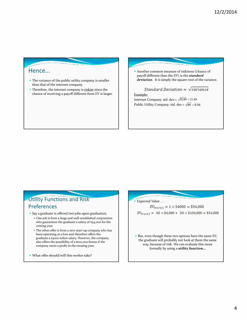
Hence…

The variance of the public utility company is smaller than that of the internet company.

Therefore, the internet company is riskier since the chance of receiving a payoff different from EV is larger. 

Another common measure of riskiness (chance of payoff different than the EV) is the standard deviation.  It is simply the square root of the variance.

Example:

Internet Company: std. dev.=

Public Utility Company: std. dev.= 

49.15240$

80 8.94

Utility Functions and Risk Preferences Say a graduate is offered two jobs upon graduation. 

One job is from a large and well‐established corporation who guarantees the graduate a salary of $54,000 for the coming year. 

The other offer is from a new start‐up company who has been operating at a loss and therefore offers the graduate a $4000 token salary. However, the company also offers the possibility of a $100,000 bonus if the company earns a profit in the ensuing year.  

What offer should/will this worker take?

Expected Value . . . 

But, even though these two options have the same EV, the graduate will probably not look at them the same 

way, because of risk. We can evaluate this more formally by using a utility function…

12/2/2014

5

Note that this utility function satisfies the usual properties of:

Increasing (more is better) in income

Diminishing marginal utility‐ slope is decreasing. 

That is, even if EVwork 1 = EVwork 2, this shows that EUwork 1 > EUwork 2, where EU is the Expected Utility

If I was offered the EV of a lottery (54) with certainty, I would prefer that (obtaining U(EV) = 230) rather than actually playing the lottery, obtaining EU = 190

B is higher than D

U(EV)

EU2

Utility from the established company

Expected utility from the start‐up company:

EV1 = EV2

Expected Utility – it is simply the expected value of the utility levels that the decision maker receives from the payoffs in the lottery. 

That is, you find the Utility from the payoff for each possible outcome of the lottery, and then find their expectation. 

We can then use this Expected Utility to see which option the decision maker would chose.

Risk Preferences Risk Averse – A characteristic of a decision maker who prefers a sure thing to a lottery of equal expected value.  That is, the decision maker above is clearly risk averse.  This is represented by all concave utility functions, i.e., utility functions that increase in income, but at a decreasing rate.  

Example…

Generally,  , where  , e.g.     As in 

12/2/2014

6

Risk averse individuals Out of 2 lotteries (or stocks, or job offers) with the sameEV, a risk averse individual selects that with the lowestvariance (e.g., the job with the sure salary rather than therisky one).

Because of diminishing marginal utility, the reduction inutility that this individual suffers from the downside of thelottery ($230‐60=170) is larger than the increase in utilityfrom the upside of the lottery ($320‐230=$90).

With utility function 

Expected Utility of Internet Company  Stock:

Expected Utility of Public Utility:

Since the EUpublic‐utility > EUinternetstock then a risk‐averse person will choose to purchase the public utility stock

EUInternet

EUPublic

Risk averse individuals Hence, if two lotteries

Have the same EV, i.e., EV1=EV2, but…

Variance1>Variance2

We can then anticipate that a risk averse individualwill find that

EU2>EU1

And therefore the risk averse individual prefers thelottery with the lowest variance.

Risk Neutral – A characteristic of a decision maker who compares lotteries according to their expected value (not EU) and is therefore indifferent between a sure thing and a lottery with the same expected value.

This is characterized by a linear utility function, example:  , where a > 0 and b > 0

12/2/2014

7

1) Marginal Utility is constant (slope of utility function is constant).2) Example: U(I)= a+bI, where MUI=b (constant).

Example , where a=0, b=100, i.e., 

EU of internet stock

EU of Public Utility

That is, when an individual is indifferent between two lotteries that, despite having the same EV, have different variances, we refer to this individual as “risk neutral.”

EUInt=EUPublic Util Risk Neutral

Risk Loving ‐ A characteristic of a decision maker who prefers a lottery to a sure thing that is equal to the expected value of the lottery. In the job offer example, a risk‐loving person would prefer the start‐up company to the established company. 

This is characterized by increasing marginal utility

Generally, the utility function is convex in income, as follows:

Let’s see this property in a figure

,  where β > 1

e.g., β = 2, A = 50

Utility

Income

                            

Utility from income of a risk‐loving individual

A

B

C

IA EV IE

$4,000 $54,000 $104,000

D

Expected utility from the start‐up company

Expected utility from the established 

company

U(I)

SummaryNote: The utility function U(I) must be:  Concave ‐> Risk‐averse

     Linear ‐> Risk neutral     Convex ‐> Risk loving

12/2/2014

8

Example‐ Risk LoverU(I) 100 I 2

a) Exp. Utility from the Internet Stock:

000,024,1

)120100(3.0)100100(4.0)80100(3.0 222

b) Exp. Utility from the Public Utility Stock:

000,008,1

)120100(1.0)100100(8.0)80100(1.0 222

Of course, the risk lover prefers the stock with the highest variance. 

If EV1=EV2 but Variance1>Variance2, then a risk lover prefers lottery (or stock, or job) 1 to lottery 2. 

That is, EU1>EU2

Bearing and Eliminating Risk We have described lotteries and how to calculate expected utilities to determine a consumer’s preferences amongst different lotteries.

We will now move into analyzing when an agent will choose to bear risk and when he will choose to eliminate it.

In particular, an agent might choose to take the riskier offer if the expected payoff from the gamble is sufficiently larger than that of the sure thing.  

Let’s start…

If the EV of the lottery is above the EV of the sure thing, we have

EULottery > EUSureThing

Initially, a risk averse decision maker preferred the sure thing rather than the lottery when EVLottery = EVSureThing.

However, if we decrease EVSureThing enough, at some point the decision maker will be indifferent between the lottery and the sure thing. That is,

EULottery = EUSureThing

12/2/2014

9

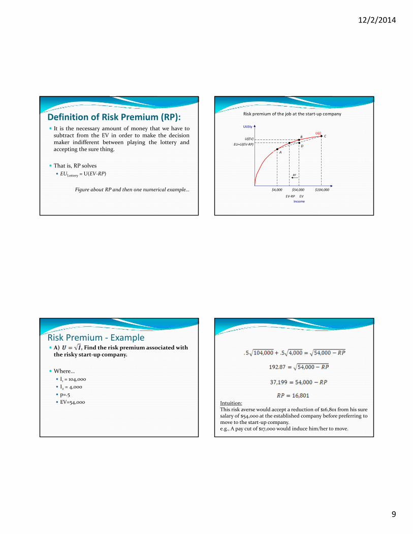
Definition of Risk Premium (RP): It is the necessary amount of money that we have tosubtract from the EV in order to make the decisionmaker indifferent between playing the lottery andaccepting the sure thing.

That is, RP solves

EULottery = U(EV‐RP)

Figure about RP and then one numerical example…

Utility

Income

Risk premium of the job at the start‐up company

A

B C

$4,000 $54,000 $104,000

D

U(I)

U(EV)

EU=U(EV‐RP)

RP

EVEV‐RP

Risk Premium ‐ Example A)  , Find the risk premium associated with the risky start‐up company.

Where…

I1 = 104,000

I2 = 4,000 

p=.5  

EV=54,000 Intuition:This risk averse would accept a reduction of $16,801 from his sure salary of $54,000 at the established company before preferring to move to the start‐up company. e.g., A pay cut of $17,000 would induce him/her to move. 

12/2/2014

10

B) What if the wage offer of the start‐up company changes to I1 = 0, I2 = 108,000 (more extreme variance!), then what is the RP?

Squaring both sides,

So, as the variance of the lottery increases, the RP also increases. 

Intuitively, since the worker is risk averse, he is willing to accept a larger pay cut in his sure salary of $54,000 before 

being induced to move to the start‐up company.

First, note that EV is

EV is still $54,000

EULottery =

EULottery=U(EV‐RP)   

pU(I1)+(1‐p)U(I2)=U(54,000‐RP)

.5 104,000 .5 4,000 54,000

192.87 54,000

37,199 54,000

16,801

Intuition:This risk averse individual would accept a reduction of $16,801 from his/her sure salary of $54,000 at the established company, before preferring to move to the start‐up company.For example, a pay cut of $17,000 would induce him/her to move to the start‐up company.

Fairly Priced Insurance The logic of risk aversion also sheds light on the circumstances under which a risk‐averse person would choose to eliminate risk by buying insurance.

When the insurance policy has a premium equal to the expected value of the promised insurance payment, we call this Fairly Priced Insurance.

This image cannot currently be displayed.

What you pay every month/yearExample

Example: Fairly priced insurance Let’s consider an example where a person has to decide whether or not to purchase insurance. 

Insurance Premium = 500

Insurance Coverage (if accident occurs) = $10,000 (full coverage)

Prob of accident = .05

Prob of no accident = .95

500 = .05(10,000) + .95(0)

500=500

Hence, this insurance policy is fairly priced. 

12/2/2014

11

Insurance: No accident: 50,000‐500 = 49,500

Accident: 50,000‐500 ‐10,000 + 10,000 = 49,500

So 49,500 is a sure thing, no matter what happens

No Insurance: No Accident: 50,000 = 50,000

Accident: 50,000‐10,000 = 40,000

EV = .5(40,000) + .95(50,000) = 49,500

And so, a risk averse person will therefore pick the sure thing (buying insurance) instead of picking the lottery.

Learning‐by‐Doing 15.4 –Willingness to pay for insurance Consider your disposable income is $90,000. 

There is a 1% chance that your house may burn, and if it does, the cost of repairing it will be $80,000, reducing your disposable income to only $10,000. 

Suppose too that your utility function is U(I)=I0.5.

( )u I I

a) Would you be willing to spend $500 to purchase an insurance policy that fully insures you against your loss?

If you don’t purchase insurance, your expected utility is

If you purchase insurance at a price of $500, your disposable income becomes $89,500 whether or not your house burns.

Hence, your utility from insurance is

298$000,1001.0000,9099.0

89,500 $299.17

a) (Cont.) Since your expected utility is higher with the policy than without it, you would be willing to purchase insurance at a price of $500.

b) What is the highest price that you would be willing to pay for this insurance policy?

Let P be the highest price that you would be willing to pay. 

If you purchase the policy, your utility is

Both when the house burns and when it doesn’t, since the insurance policy fully compensates you for repairs

P000,90

12/2/2014

12

If instead you don’t purchase insurance, your expected utility is $298, ,

(we found this in part a). 

Hence, you are indifferent between purchasing and not purchasing insurance when its price P satisfies

That is, the most you’d be willing to pay for this insurance policy is $1,196.

LotteryEURPEV

PP

804,88000,90298000,90

Asymmetric Information Asymmetric Information – it is basically a situation in which one party knows more about its own actions or characteristics than another party.

For instance, you know more about your driving habits than a car insurance company. 

For this reason, car insurance companies charge a premium to safeguard against their lack of information 

Similarly, think about health insurance deductibles.

Suppose your car is fully insured. How careful would you be? Probably not as careful as you would be without 

insurance, or with partial insurance. That is, insurance in a way incentivizes less careful driving. 

This is a form of moral hazard – a phenomenon whereby an insured party exercises less care than he or she would in the absence of insurance. 

How to provide incentives for careful driving?

Including deductible into the insurance policy.

But not too big! Otherwise good drivers (if very risk averse) might not be attracted to the policy. 

Another reason insurance companies do not provide full coverage is adverse selection – a phenomenon whereby an increase in the premium increases the overall riskiness of the pool of individuals who buy an insurance policy. 

That is, the higher the premium the insurance company charges, the more likely that only people truly in need of insurance (reckless car drivers, unhealthy people, etc.) will buy the policy

12/2/2014

13

How to avoid adverse selection?

One solution: Offering a “menu” of insurance policies to customers, and allow each customer to select the particular policy that he/she most prefers.

A policy with a large deductible and low premium would appeal to someone who is convinced his/her chances of illness are low, whereas…

A policy with a small deductible and high premium would appeal to someone who is convinced that his/her chances of illness are high.

How to avoid adverse selection?

Another solution: 

Pooling good and bad risks together: 

For instance, if all employees in a company participate in a mandatory companywide health insurance plan, the insurance company offering the group plan will face a mix of high and low‐risk individuals, reducing its costs as a consequence.

Decision trees A Decision tree is a diagram that describes theoptions available to a decision maker…

as well as the risky events that can occur at each point intime.

Let’s see one simple example for an oil company thathas just discovered a new reserve of oil

(next page).

Company

Chance

Chance

Build small

Build large

Reservoir is small

Reservoir is large

Reservoir is large

Reservoir is small

p=1/2

1‐p=1/2

q=1/2

1‐q=1/2

Oil company’s payoff

$50

$10

$30

$20

12/2/2014

14

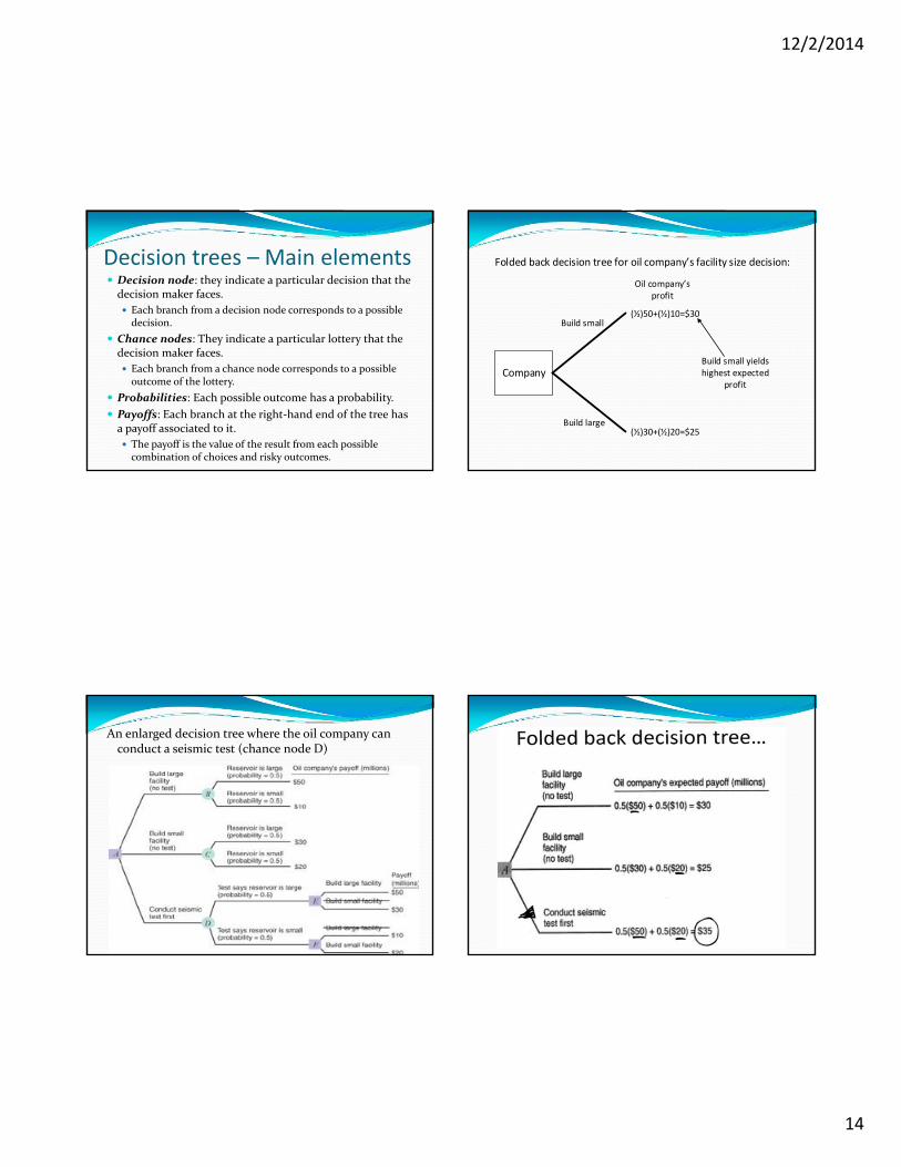
Decision trees – Main elements Decision node: they indicate a particular decision that the decision maker faces. 

Each branch from a decision node corresponds to a possible decision.

Chance nodes: They indicate a particular lottery that the decision maker faces. 

Each branch from a chance node corresponds to a possible outcome of the lottery.

Probabilities: Each possible outcome has a probability.

Payoffs: Each branch at the right‐hand end of the tree has a payoff associated to it. 

The payoff is the value of the result from each possible combination of choices and risky outcomes. 

Company

Build small

Build large

Folded back decision tree for oil company’s facility size decision:

(½)50+(½)10=$30

(½)30+(½)20=$25

Oil company’s profit

Build small yields highest expected 

profit

An enlarged decision tree where the oil company can conduct a seismic test (chance node D)

12/2/2014

15

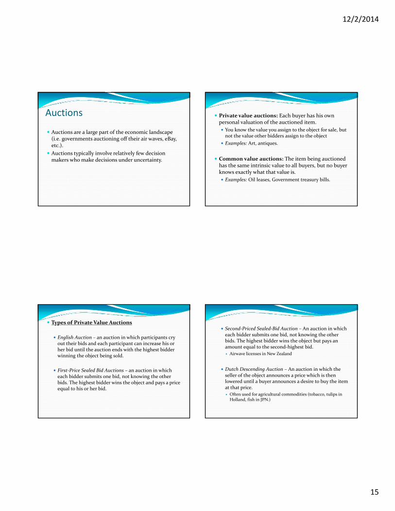
Auctions

Auctions are a large part of the economic landscape (i.e. governments auctioning off their air waves, eBay, etc.).  

Auctions typically involve relatively few decision makers who make decisions under uncertainty.  

Private value auctions: Each buyer has his own personal valuation of the auctioned item. 

You know the value you assign to the object for sale, but not the value other bidders assign to the object 

Examples: Art, antiques. 

Common value auctions: The item being auctioned has the same intrinsic value to all buyers, but no buyer knows exactly what that value is. 

Examples: Oil leases, Government treasury bills. 

Types of Private Value Auctions

English Auction – an auction in which participants cry out their bids and each participant can increase his or her bid until the auction ends with the highest bidder winning the object being sold. 

First‐Price Sealed Bid Auctions – an auction in which each bidder submits one bid, not knowing the other bids. The highest bidder wins the object and pays a price equal to his or her bid.  

Second‐Priced Sealed‐Bid Auction – An auction in which each bidder submits one bid, not knowing the other bids. The highest bidder wins the object but pays an amount equal to the second‐highest bid.

Airwave licenses in New Zealand 

Dutch Descending Auction – An auction in which the seller of the object announces a price which is then lowered until a buyer announces a desire to buy the item at that price. 

Often used for agricultural commodities (tobacco, tulips in Holland, fish in JPN.)

12/2/2014

16

Auctions N bidders, each bidder i with a valuation vi for the object.

One seller.

We can design many different rules for the auction:

1. First price auction: the winner is the bidder submitting the highest bid, and he/she must pay the highest bid (which is his/hers).

2. Second price auction: the winner is the bidder submitting the highest bid, but he/she must pay the second highest bid.

3. Third price auction: the winner is the bidder submitting the highest bid, but he/she must pay the third highest bid.

4. All‐pay auction: the winner is the bidder submitting the highest bid, but every single bidder must pay the price he/she submitted.

Auctions Note that all auctions can be interpreted as allocation mechanisms: each auction specifies1. An allocation rule (who gets the object):

1. The allocation rule for most auctions determines the object is allocated to the individual submitting the highest bid. However, we could assign the object by a lottery, where 

⋯as in “Chinese auctions”.

2. A payment rule (how much every bidder must pay):1. The payment rule in the FPA determines that the individual 

submitting the highest bid pays his/her bid, while everybody else pays zero.

2. The payment rule in the SPA determines that the individual submitting the highest bid pays the second highest bid, while everybody else pays zero.

3. The payment rule in the APA determines that every individual must pay the bid he/she submitted.

Auctions Auctions as incomplete information games:

1. I know my valuation for the object, vi, but…

2. I don’t know your valuation for the object, vj, but I know that it is drawn from a distribution function.

1. Easiest case:10withprobability0.4, or5withprobability0.6

2. Moregenerally,c.d.f.  F(v) = prob(vj<v)

3. We will normally assume that every bidder’s valuation for the object is drawn from a uniform distribution function between 0and 1,  0,1 .

3. Symmetry in the bidding function:∶ 0,1 → foreverybidderi

Cumulative Probability,F(v)

vj

1

10

Prob(vj>v)=1‐F(v)=1‐v

Prob(vj<v)=F(v)=v

v

v

vj<v vj>v

12/2/2014

17

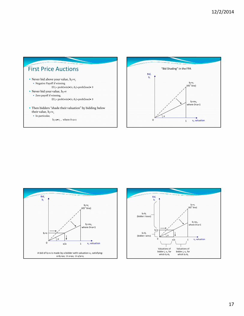
First Price Auctions

Never bid above your value, bi>vi Negative Payoff if winning

EUi= prob(win)(vi‐bi)+prob(lose) 0

Never bid your value, bi=v

Zero payoff if winning, 

EUi= prob(win)(vi‐bi)+prob(lose) 0

Then bidders “shade their valuation” by bidding below their value, bi<vi. In particular,

bi=avi ,  where 0<a<1

Bid, bj

vj, valuation10

bj=vj(45o line)

bj=avj,where 0<a<1

a

“Bid Shading” in the FPA

Bid, bj

vj, valuation10

bj=vj(45o line)

bj=avj,where 0<a<1

a

bi=x

x/a

A bid of bi=x is made by a bidder with valuation vi, satisfying:x=bi=avi → x=avi → x/a=vi

Bid, bj

vj, valuation10

bj=vj(45o line)

bj=avj,where 0<a<1

a

bi=x

x/a

bi<bj

(bidder i loses)

bi>bj

(bidder i wins)

Valuations of bidder j, vj, for which bi>bj

Valuations of bidder j, vj, for which bi<bj

12/2/2014

18

What is the probability of winning?

Of course, prob(win)= prob(bi>bj)

And, according to the previous figure,

prob(bi>bj)=prob(x>bj)

And  from the point of view of valuations (horizontal 

axis), prob(x>bj)=prob( >vj)

See shaded region of vertical axis

See shaded region of horizontal axis

Assuming that all valuations are uniformly distributed between 0 and 1, prob( )=

Recall that: 

Prob(x>vj)=x

Prob(x<vj)=1‐x

We are now ready to write the bidder’s expected utility bi=x, for a given valuation vi,

EUi(bi|vi)=(vi‐x)xa+0(1‐xa)

=vix−x

2

a

vj0

x

1

x 1‐x

Payoff if winning

Payoff if losing

Prob of winning

Prob of losing

Taking F.O.C. with respect to bidder i’s bid, x,

0 2

And solving for the bid x, we obtain the optimal bidding function

12

That is, the bidder submits bid equal to half of his valuation for the object.

Bid, bj

vj, valuation10

bj=vj(45o line)

bi=½vi,

1/2

1/2

1

Optimal bidding function   

12/2/2014

19

What if we are dealing with N bidders?

Prob(win)=prob(xa v

1)prob(xa v )…prob(xa v )

prob(xa v )…prob(xa v )

= xa xa… xa = (

xa )

 

Therefore, the EUi is: 

EUi(bi|vi)=(vi‐x)(xa )

  + 0 [1‐( xa ) 

Payoff if winning

Payoff if losing

Prob of winning

Prob of losing

Taking F.O.C. with respect to bid x:

‐(xa )

  +(vi‐x)(n‐1)(xa )

  1a = 0

Rearranging,

1x a(

xa )

  [(n‐1)vi‐nx]= 0

And solving for x,

(n‐1)vi=nx

x(vi)=n 1n vi

Optimal bidding function

Note that for very large N, e.g., N=2,000, we have bi=,

,vi, 

and bivi (almost coinciding with the bidder’s valuation, in 45o line, i.e., very small “bid shading”).

Bid, bi

vi, valuation10

bi=vi(45o line)

bi=½vi (if N=2)½ 

1

¾ 

⅔ 

bi=¾vi (if N=4)

bi=⅔vi (if N=3)

Second Price Auction, SPA

Bidding your valuation, bi=vi, is a weakly dominant strategy for all players.

That is, there is no other bidding strategy that provides a bidder with a strictly larger payoff. 

In other words, all other strategies yield a lower or equal payoff as bidding my own valuation, bi=vi.

12/2/2014

20

Second Price Auction, SPA Let’s show it by comparing the payoffs from bidding bi=vi versus any other bidding strategy.

1. If the bidder bids bi=vi, then either

a) hi>bi, and he loses the auction, or

b) hi<bi, and he wins with a payoff vi‐hi, or

c) hi=bi, a tie, then the object is randomly assigned

½(vi‐hi)

(Or among the number of K bidders submitting the same highest bid)

2. If the bidder shades his bid, bi<vi, then either

a) hi>bi, and he loses the auction, or

b) hi<bi, and he wins with a payoff vi‐hi, or

c) hi=bi, a tie occurs, and the object is randomly assigned yielding a expected payoff of ½(vi‐hi)

bihi

(+) Payoff(‐) Payoff vi

2. If the bidder bids above his valuation, bi>vi, either

a) hi>bi, and he loses the auction, or

b) hi<bi, and he wins, and:

He gets a payoff of vi‐hi>0 if vi>hi, or

He gets a negative payoff if vi<hi.

c) hi=bi, a tie, with the expected payoff:

½(vi‐hi)> 0 if vi>hi

½(vi‐hi)< 0 if vi<hi

bihi

(+) Payoff(‐) Payoff vi Second‐price auctions Summary:

Hence, there is no bidding strategy providing a strictly higher payoff than bi=vi in the SPA.

Efficiency:

1. In auctions, we say that an auction (or any allocation mechanism) is efficient if the bidder with the highest valuation for the object is indeed the person receiving the object.

2. In this sense, both the FPA and the SPA are efficient.

12/2/2014

21

English auction Easy!

They are equivalent to second‐price auctions (SPA) since…

If you are the bidder with the highest willingness to pay for the good, you increase your bid until the last bidder drops and…

You pay just a few bit more than the second highest bid (the last bid your closest competitor submitted).

Common Value Auctions:

When bidders have common values, a complication arises that does not occur when bidders have private values, the winner’s curse: The winning bidder might bid an amount that exceeds the item’s intrinsic value

True value! My bid (some bid shading)

My estimate

Winner’s curse In auctions where all bidders assign the same valuation to the object (common value auctions), and where every bidder receives an inexact signal of the object’s true value…

The fact that you won just means that you received an overestimated signal of the true value of the object for sale (oil lease).

How to avoid the winner’s curse?

Bid b=s‐2 or less, in order to take into account the possibility that you receive an overestimated signal.

Winner’s curse Empirically tested:

The winner’s curse in the classroom: 

A jar of nickels which every student can look at for a few minutes before submitting his/her bid

12/2/2014

22

Winner’s curse Empirically tested:

The winner’s curse in the field:

Texaco in auctions selling mineral rights to off‐shore properties owned by the US government. 

All firms avoided the winner’s curse, except for Texaco.

Were the executives sent back to school for some remedial microeconomics?

More on auction theory and related topics on…

Course on

Strategy and Game Theory 

EconS 424 – Spring 2015