Chap004 - North Seattle Collegefaculty.northseattle.edu/wholt/bus210/files/powerpoint/bus210_Ch04.pdf · 9/28/12 4 4-19 • Useful for comparing variables measured in different units

9/28/12

1

McGraw-Hill/Irwin Copyright © 2013 by The McGraw-Hill Companies, Inc. All rights reserved.

A PowerPoint Presentation Package to Accompany

Applied Statistics in Business & Economics, 4th edition

David P. Doane and Lori E. Seward

Prepared by Lloyd R. Jaisingh

4-2

Descriptive Statistics

Chapter Contents

4.1 Numerical Description 4.2 Measures of Center 4.3 Measures of Variability 4.4 Standardized Data 4.5 Percentiles, Quartiles, and Box Plots 4.6 Correlation and Covariance 4.7 Grouped Data 4.8 Skewness and Kurtosis

Chapter 4

4-3

Chapter Learning Objectives LO4-1: Explain the concepts of center, variability, and shape.

LO4-2: Use Excel to obtain descriptive statistics and visual displays.

LO4-3: Calculate and interpret common measures of center.

LO4-4: Calculate and interpret common measures of variability.

LO4-5: Transform a data set into standardized values.

LO4-6: Apply the Empirical Rule and recognize outliers.

Chapter 4


4-4

Chapter Learning Objectives LO4-7: Calculate quartiles and other percentiles.

LO4-8: Make and interpret box plots.

LO4-9: Calculate and interpret a correlation coefficient and covariance.

LO4-10: Calculate the mean and standard deviation from grouped data.

LO4-11: Assess skewness and kurtosis in a sample.

Chapter 4


4-5

Chapter 4

4.1 Numerical Description

LO4-1: Explain the concepts of center, variability, and shape.

Three key characteristics of numerical data:

LO4-1

4-6

Chapter 4

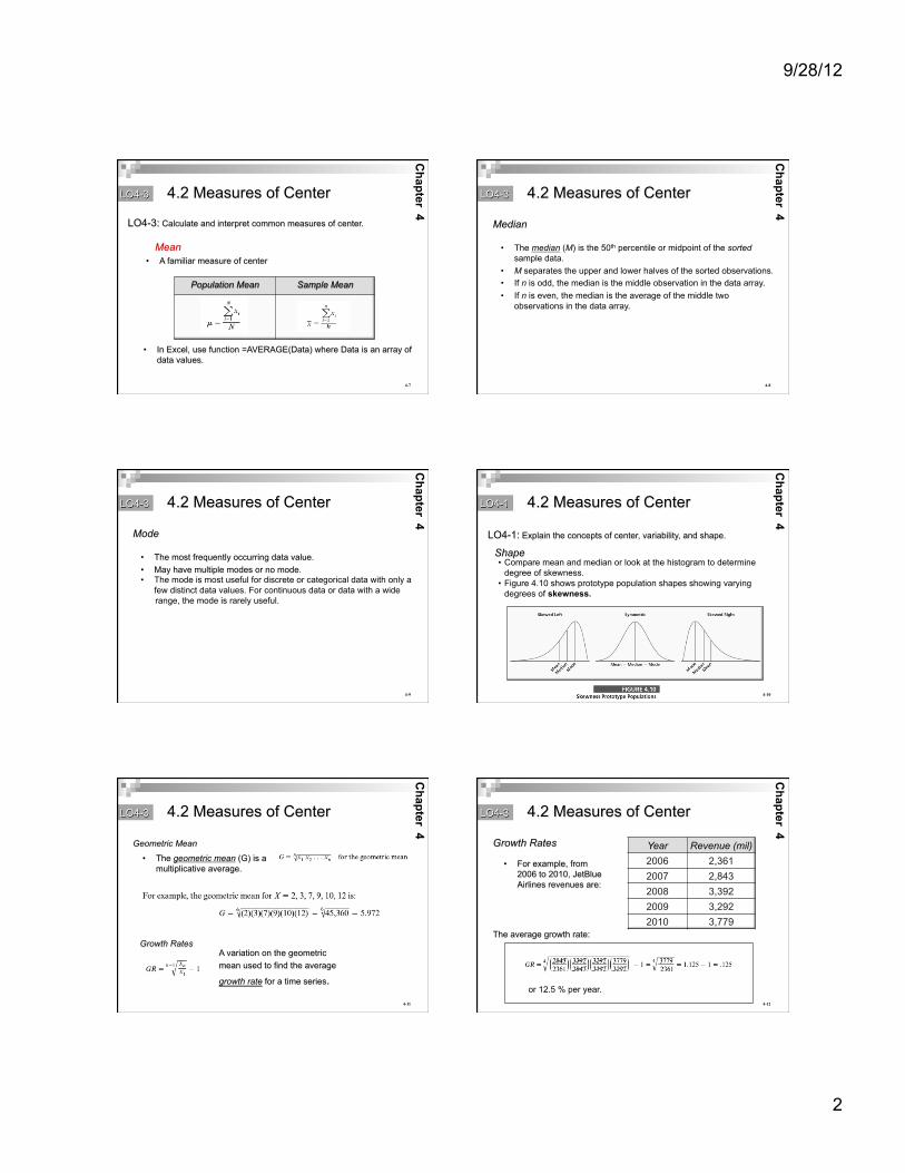
LO4-2: Use Excel to obtain descriptive statistics and visual displays.

LO4-2

EXCEL Histogram Display for Tables 4.3

4.1 Numerical Description

9/28/12

2

4-7

•  A familiar measure of center

•  In Excel, use function =AVERAGE(Data) where Data is an array of data values.

Population Mean Sample Mean

Mean

Chapter 4

4.2 Measures of Center LO4-3

LO4-3: Calculate and interpret common measures of center.

4-8

•  The median (M) is the 50th percentile or midpoint of the sorted sample data.

•  M separates the upper and lower halves of the sorted observations. •  If n is odd, the median is the middle observation in the data array. •  If n is even, the median is the average of the middle two

observations in the data array.

Median

Chapter 4

LO4-3 4.2 Measures of Center

4-9

•  The most frequently occurring data value. •  May have multiple modes or no mode. •  The mode is most useful for discrete or categorical data with only a

few distinct data values. For continuous data or data with a wide range, the mode is rarely useful.

Mode

Chapter 4


4-10

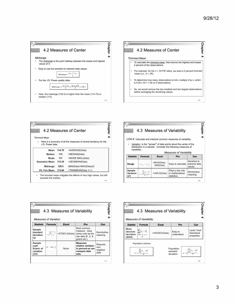
•  Compare mean and median or look at the histogram to determine degree of skewness.

•  Figure 4.10 shows prototype population shapes showing varying degrees of skewness.

Shape

Chapter 4

LO4-1: Explain the concepts of center, variability, and shape.


4-11

•  The geometric mean (G) is a multiplicative average.

Geometric Mean

Chapter 4

Growth Rates A variation on the geometric mean used to find the average

growth rate for a time series.


4-12

•  For example, from 2006 to 2010, JetBlue Airlines revenues are:

Year Revenue (mil) 2006 2,361 2007 2,843 2008 3,392 2009 3,292 2010 3,779

Growth Rates

The average growth rate:

or 12.5 % per year.

Chapter 4


9/28/12

3

4-13

•  The midrange is the point halfway between the lowest and highest values of X.

•  Easy to use but sensitive to extreme data values.

•  Here, the midrange (126.5) is higher than the mean (114.70) or median (113).

Midrange

•  For the J.D. Power quality data:

Chapter 4


4-14

•  To calculate the trimmed mean, first remove the highest and lowest k percent of the observations.

•  For example, for the n = 33 P/E ratios, we want a 5 percent trimmed mean (i.e., k = .05).

•  To determine how many observations to trim, multiply k by n, which is 0.05 x 33 = 1.65 or 2 observations.

•  So, we would remove the two smallest and two largest observations before averaging the remaining values.

Trimmed Mean

Chapter 4


4-15

•  Here is a summary of all the measures of central tendency for the J.D. Power data.

•  The trimmed mean mitigates the effects of very high values, but still exceeds the median.

Mean: 114.70 =AVERAGE(Data)

Median: 113 =MEDIAN(Data)

Mode: 111 =MODE.SNGL(Data) Geometric Mean: 113.35 =GEOMEAN(Data)

Midrange: 126.5 (MIN(Data)+MAX(Data))/2

5% Trim Mean: 113.94 =TRIMMEAN(Data, 0.1)

Trimmed Mean

Chapter 4


4-16

•  Variation is the “spread” of data points about the center of the distribution in a sample. Consider the following measures of variability:

Statistic Formula Excel Pro Con

Range xmax – xmin =MAX(Data) -

MIN(Data) Easy to calculate Sensitive to extreme data values.

Sample Variance (s2)

=VAR.S(Data) Plays a key role in mathematical statistics.

Nonintuitive meaning.

Measures of Variability

Chapter 4

4.3 Measures of Variability

LO4-4: Calculate and interpret common measures of variability.

LO4-4

4-17


Sample standard deviation (s)

=STDEV.S(Data)

Most common measure. Uses same units as the raw data ($ , £, ¥, grams etc.).

Nonintuitive meaning.

Measures of Variation

Sample coef-ficient. of variation (CV)

None

Measures relative variation in percent so can compare data sets.

Requires non-negative data.

Chapter 4

LO4-4 4.3 Measures of Variability

4-18


Mean absolute deviation (MAD)

=AVEDEV(Data) Easy to understand.

Lacks “nice” theoretical properties.

Measures of Variability

1

n

iix x

n=

−∑

Population variance

Population standard deviation

Chapter 4

4.3 Measures of Variability LO4-4

9/28/12

4

4-19

•  Useful for comparing variables measured in different units or with different means.

•  A unit-free measure of dispersion.

•  Expressed as a percent of the mean.

•  Only appropriate for nonnegative data. It is undefined if the mean is zero or negative.

Coefficient of Variation

Chapter 4


4-20

•  This statistic reveals the average distance from the center.

•  Absolute values must be used since otherwise the deviations around the mean would sum to zero. It is stated in the unit of measurement.

•  The MAD is appealing because of its simple interpretation.

Mean Absolute Deviation

Chapter 4


4-21

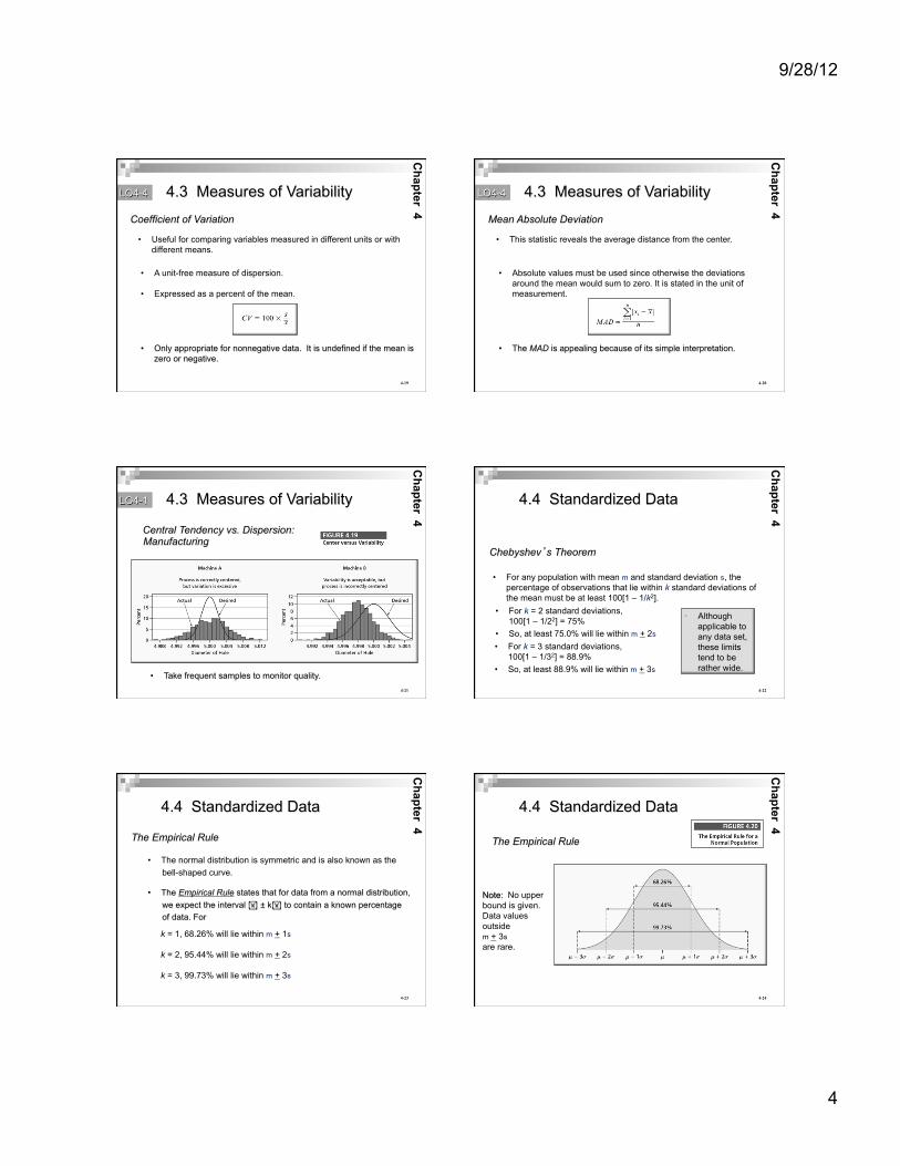
•  Take frequent samples to monitor quality.

Central Tendency vs. Dispersion: Manufacturing

Chapter 4


4-22

•  For any population with mean m and standard deviation s, the percentage of observations that lie within k standard deviations of the mean must be at least 100[1 – 1/k2].

Chebyshev’s Theorem

•  For k = 2 standard deviations, 100[1 – 1/22] = 75%

•  So, at least 75.0% will lie within m + 2s •  For k = 3 standard deviations,

100[1 – 1/32] = 88.9% •  So, at least 88.9% will lie within m + 3s

•  Although applicable to any data set, these limits tend to be rather wide.

Chapter 4

4.4 Standardized Data

4-23

•  The Empirical Rule states that for data from a normal distribution, we expect the interval ± k to contain a known percentage of data. For

•  The normal distribution is symmetric and is also known as the bell-shaped curve.

k = 1, 68.26% will lie within m + 1s



The Empirical Rule

Chapter 4


4-24

Note: No upper bound is given. Data values outside m + 3s are rare.

The Empirical Rule

Chapter 4


9/28/12

5

4-25

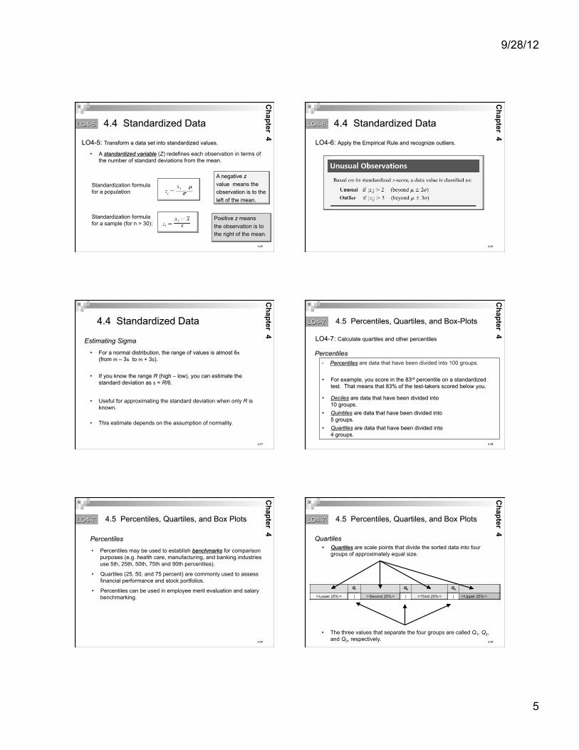
•  A standardized variable (Z) redefines each observation in terms of the number of standard deviations from the mean.

A negative z value means the observation is to the left of the mean.

Positive z means the observation is to the right of the mean.

Chapter 4

4.4 Standardized Data LO4-5

Standardization formula for a population:

Standardization formula for a sample (for n > 30):

LO4-5: Transform a data set into standardized values.

4-26

Chapter 4 LO4-6: Apply the Empirical Rule and recognize outliers.

LO4-6 4.4 Standardized Data

4-27

•  For a normal distribution, the range of values is almost 6s (from m – 3s to m + 3s).

•  If you know the range R (high – low), you can estimate the standard deviation as s = R/6.

•  Useful for approximating the standard deviation when only R is known.

•  This estimate depends on the assumption of normality.

Estimating Sigma

Chapter 4


4-28

•  Percentiles are data that have been divided into 100 groups.

•  For example, you score in the 83rd percentile on a standardized test. That means that 83% of the test-takers scored below you.

•  Deciles are data that have been divided into 10 groups.

•  Quintiles are data that have been divided into 5 groups.

•  Quartiles are data that have been divided into 4 groups.

Percentiles

Chapter 4

4.5 Percentiles, Quartiles, and Box-Plots

LO4-7: Calculate quartiles and other percentiles

LO4-7

4-29

•  Percentiles may be used to establish benchmarks for comparison purposes (e.g. health care, manufacturing, and banking industries use 5th, 25th, 50th, 75th and 90th percentiles).

•  Quartiles (25, 50, and 75 percent) are commonly used to assess financial performance and stock portfolios.

•  Percentiles can be used in employee merit evaluation and salary benchmarking.

Percentiles

Chapter 4

LO4-7 4.5 Percentiles, Quartiles, and Box Plots

4-30

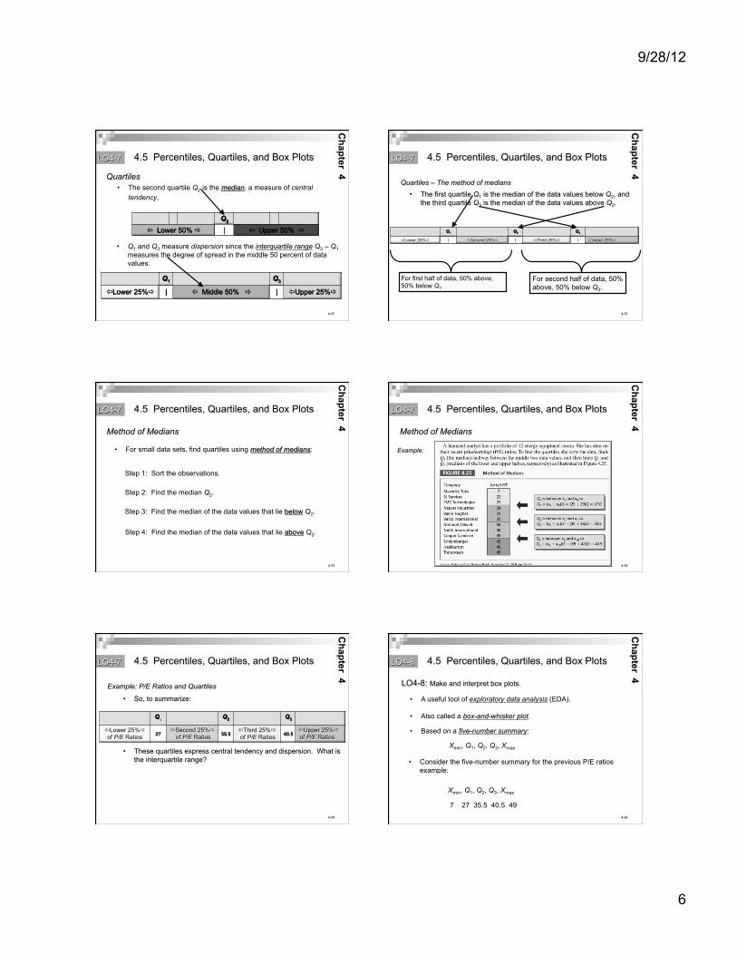
•  Quartiles are scale points that divide the sorted data into four groups of approximately equal size.

•  The three values that separate the four groups are called Q1, Q2, and Q3, respectively.

Q1 Q2 Q3

ïLower 25%ð | ïSecond 25%ð | ïThird 25%ð | ïUpper 25%ð

Quartiles

Chapter 4


9/28/12

6

4-31

•  The second quartile Q2 is the median, a measure of central tendency.

•  Q1 and Q3 measure dispersion since the interquartile range Q3 – Q1 measures the degree of spread in the middle 50 percent of data values.

Q2 ï Lower 50% ð | ï Upper 50% ð

Q1 Q3

ïLower 25%ð | ï Middle 50% ð | ïUpper 25%ð

Quartiles

Chapter 4


4-32

•  The first quartile Q1 is the median of the data values below Q2, and the third quartile Q3 is the median of the data values above Q2.

Q1 Q2 Q3

ïLower 25%ð | ïSecond 25%ð | ïThird 25%ð | ïUpper 25%ð

For first half of data, 50% above, 50% below Q1.

For second half of data, 50% above, 50% below Q3.

Quartiles – The method of medians

Chapter 4


4-33

•  For small data sets, find quartiles using method of medians:

Step 1: Sort the observations.

Step 2: Find the median Q2.

Step 3: Find the median of the data values that lie below Q2.

Step 4: Find the median of the data values that lie above Q2.

Method of Medians

Chapter 4


4-34

Method of Medians

Chapter 4

LO4-7

Example:

4.5 Percentiles, Quartiles, and Box Plots

4-35

•  So, to summarize:

•  These quartiles express central tendency and dispersion. What is the interquartile range?

Q1 Q2 Q3

ïLower 25%ð of P/E Ratios 27 ïSecond 25%ð

of P/E Ratios 35.5 ïThird 25%ð of P/E Ratios 40.5 ïUpper 25%ð

of P/E Ratios

Example: P/E Ratios and Quartiles

Chapter 4


4-36

•  A useful tool of exploratory data analysis (EDA).

•  Also called a box-and-whisker plot.

•  Based on a five-number summary:

Xmin, Q1, Q2, Q3, Xmax

•  Consider the five-number summary for the previous P/E ratios example:

7 27 35.5 40.5 49

Xmin, Q1, Q2, Q3, Xmax

Chapter 4 LO4-8: Make and interpret box plots.


9/28/12

7

4-37

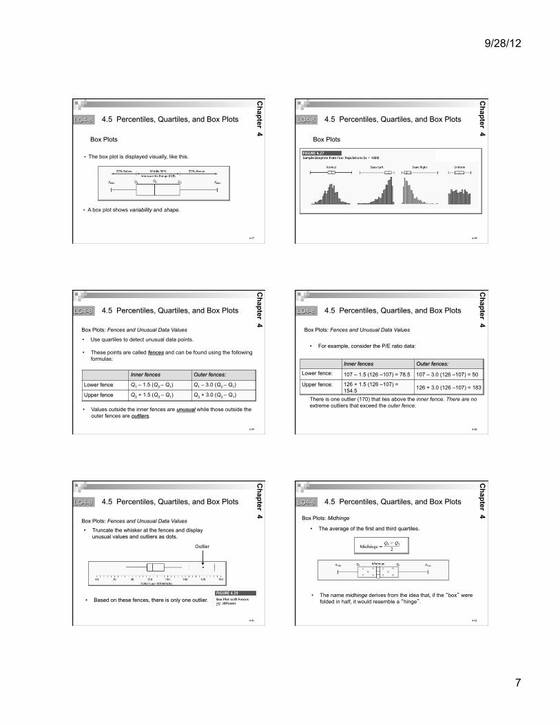
•  The box plot is displayed visually, like this.

•  A box plot shows variability and shape.

Chapter 4

Box Plots


4-38

Chapter 4

Box Plots


4-39

•  Use quartiles to detect unusual data points.

•  These points are called fences and can be found using the following formulas:

Inner fences Outer fences:

Lower fence Q1 – 1.5 (Q3 – Q1) Q1 – 3.0 (Q3 – Q1)

Upper fence Q3 + 1.5 (Q3 – Q1) Q3 + 3.0 (Q3 – Q1)

•  Values outside the inner fences are unusual while those outside the outer fences are outliers.

Box Plots: Fences and Unusual Data Values

Chapter 4


4-40

•  For example, consider the P/E ratio data:

There is one outlier (170) that lies above the inner fence. There are no extreme outliers that exceed the outer fence.

Inner fences Outer fences:

Lower fence: 107 – 1.5 (126 –107) = 78.5 107 – 3.0 (126 –107) = 50

Upper fence: 126 + 1.5 (126 –107) = 154.5 126 + 3.0 (126 –107) = 183

Box Plots: Fences and Unusual Data Values

Chapter 4


4-41

•  Truncate the whisker at the fences and display unusual values and outliers as dots.

•  Based on these fences, there is only one outlier.

Chapter 4 Box Plots: Fences and Unusual Data Values

LO4-8

Outlier

4.5 Percentiles, Quartiles, and Box Plots

4-42

•  The average of the first and third quartiles.

•  The name midhinge derives from the idea that, if the “box” were folded in half, it would resemble a “hinge”.

Box Plots: Midhinge

Chapter 4


9/28/12

8

4-43

•  The sample correlation coefficient is a statistic that describes the degree of linearity between paired observations on two quantitative variables X and Y.

Correlation Coefficient

Note: -1 ≤ r ≤ +1.

Chapter 4

4.6 Correlation and Covariance

LO4-9: Calculate and interpret a correlation coefficient and covariance.

LO4-9

4-44

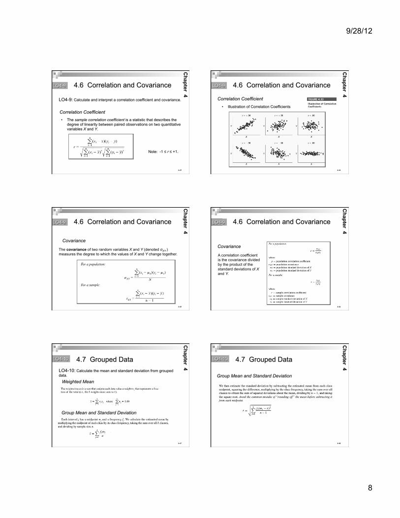
•  Illustration of Correlation Coefficients

Correlation Coefficient

Chapter 4

LO4-9 4.6 Correlation and Covariance

4-45

The covariance of two random variables X and Y (denoted σXY ) measures the degree to which the values of X and Y change together.

Covariance

Chapter 4

LO4-9 4.6 Correlation and Covariance

4-46

A correlation coefficient is the covariance divided by the product of the standard deviations of X and Y.

Covariance

Chapter 4

LO LO4-9 4.6 Correlation and Covariance

4-47

Group Mean and Standard Deviation

Chapter 4

4.7 Grouped Data LO4-10: Calculate the mean and standard deviation from grouped data.

LO4-10

Weighted Mean

4-48

Group Mean and Standard Deviation

Chapter 4

LO4-10 4.7 Grouped Data

9/28/12

9

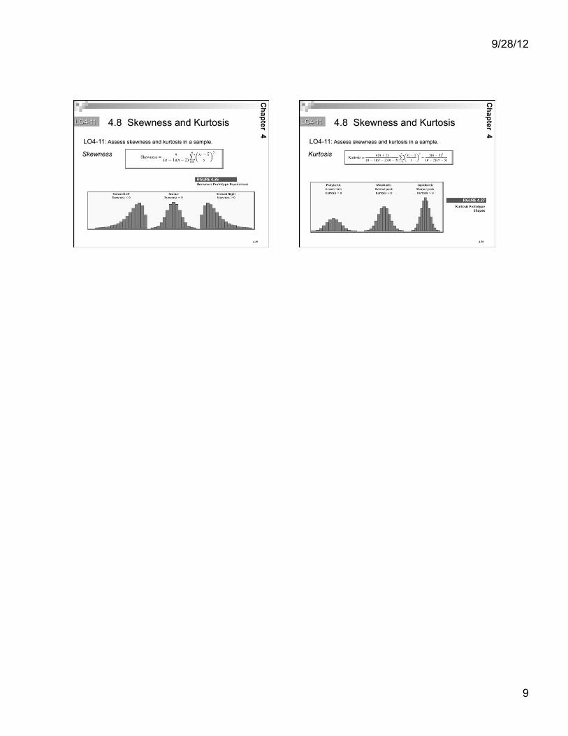
4-49

Skewness

Chapter 4

4.8 Skewness and Kurtosis


LO4-11

4-50

Kurtosis

Chapter 4

LO4-11


4.8 Skewness and Kurtosis

Documents

Chap004 - North Seattle Collegefaculty.northseattle.edu/wholt/bus210/files/powerpoint/bus210_Ch04.pdf · 9/28/12 4 4-19 • Useful for comparing variables measured in different units