Page 1 of 17

Managing Six Sigma: Understanding the Importance of Self Study

By Dean Christolear

Chapter Three - Analyze

The Specification for the shaft is 18.85 +/- 0.10 mm. Rougher 1 appears to be making

good parts. Rougher 2 appears to have a large amount of variation and is making a lot of

undersized parts. Rougher 3 is also making some undersize parts but does not appear to

have the large amount of variation exhibited by Rougher 2.

18.5

18.55

18.6

18.65

18.7

18.75

18.8

18.85

18.9

18.95

19

Rougher 1 Rougher 2 Rougher 3

Lower Quartile

Minimum

Median

Maximum

Upper Quartile

You share the information with the production supervisor, and he is suspicious of the

gage on Roughers 2 and 3. He calls for the gages to be re-mastered. The gage man

informs the supervisor that the gages were not mastered correctly and were under by

about 0.05 to 0.06 mm. The gages are now back in service and Rougher 2 and 3 are

retargeted.

Page 2 of 17

Rougher 2 presents a different problem. The targeting issue has been corrected but the

variation is so great that there will always be parts out of specification on the high and

low ends of the tolerance.

Return to the file Rougher check sheets.xls and go to Sheet 1 where you

previously generated the box plot. Highlight the entire column for Rougher 2 (including

the header) beginning in Cell B25. NOTE: Do not paint any data in the first 24 rows

where the Box plot calculations and charting were performed. This will cause errors in

your charting.

Insert a Run chart as you did before. You can find an excellent reference on Run charts

at http://quality.disa.mil/pdf/runchart.pdf. You are expected to have a thorough

understanding of this tool.

Once completed, your Run chart should look like this.

Rougher 2

18.518.5518.6

18.6518.7

18.7518.8

18.8518.9

18.9519

1 18 35 52 69 86 103 120 137 154 171 188 205 222 239 256

Page 3 of 17

There do not appear to be any cycles, trends or shifts that might point to issues with the

machine or with differences between shifts. In order to perform a more thorough

analysis, you decide to do a Capability Study. A Capability Study is a formal analysis

that will fully demonstrate the ability (or lack of ability) of Rougher 2 to manufacture

parts within specification.

You can find an excellent reference on Process Capability at

http://www.itl.nist.gov/div898/handbook/ppc/section4/ppc46.htm. You are expected to

have a thorough understanding of this tool.

In order to begin the analysis you will need to calculate the following values:

The average of the data set, also called the “mean”;

The standard deviation of the data set, and

The tolerance range of the part, sometimes called “engineering tolerance.”

The tolerance range is easily calculated by subtracting the minimum allowable shaft size

from the maximum allowable shaft size. The average and standard deviation can be

calculated using the functions AVERAGE and STDEV; however, we will use the Data

Analysis ToolPak in Excel®.

Page 4 of 17

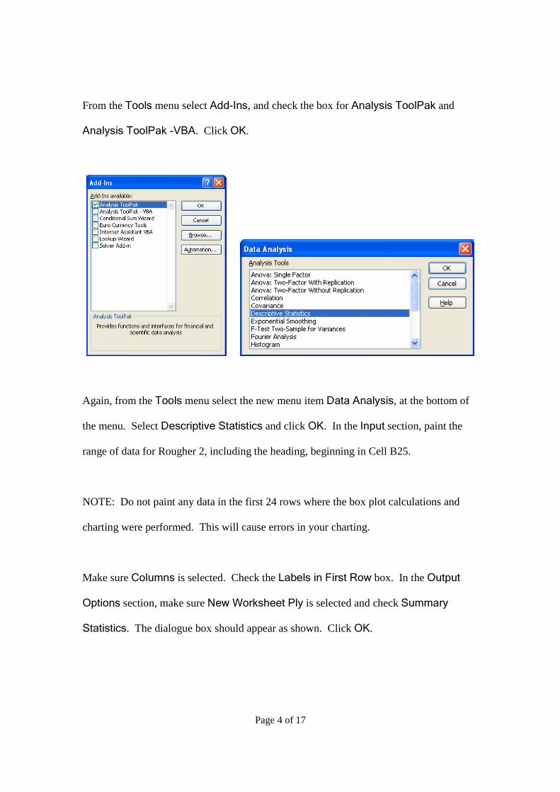
From the Tools menu select Add-Ins, and check the box for Analysis ToolPak and

Analysis ToolPak -VBA. Click OK.

Again, from the Tools menu select the new menu item Data Analysis, at the bottom of

the menu. Select Descriptive Statistics and click OK. In the Input section, paint the

range of data for Rougher 2, including the heading, beginning in Cell B25.

NOTE: Do not paint any data in the first 24 rows where the box plot calculations and

charting were performed. This will cause errors in your charting.

Make sure Columns is selected. Check the Labels in First Row box. In the Output

Options section, make sure New Worksheet Ply is selected and check Summary

Statistics. The dialogue box should appear as shown. Click OK.

Page 5 of 17

A new worksheet ply will be added to your spreadsheet--most likely labeled Sheet 2--

with a number of descriptive statistics. You may need to widen Column A. Select it by

clicking on the “A” column heading. Select Format, Column, Width. A value of 20

should allow you to view the entries in Column A completely.

Page 6 of 17

The resultant values for average and standard deviation are seen to be included among the

descriptive statistics. In the open cells below the descriptive statistics, enter the

following labels in column A:

USL

LSL

Tolerance Range

Cp

Cpk Upper

Cpk Lower

Cpk

You will be calculating many of these values in Excel® by using formulas. In an Excel®

formula, the following operations are performed using the keys shown:

Addition Plus Sign +

Subtraction Minus Sign, Hyphen -

Multiplication Asterisk *

Division Forward Slash /

Start the formula Equal Sign =

Page 7 of 17

If you are not already familiar with Excel® formulas, you should review them by opening

Help, Microsoft Excel Help, and clicking on Table of Contents. Navigate to Working

with Data, Formulas, About Formulas.

You should also review About Calculation Operators, which explains the order in

which Excel® performs operations in formulas.

Page 8 of 17

A thorough understanding of Excel® formulas is required for the remaining portions of

this study program.

In Column B enter the values for the Upper Specification Limit (“USL”) and the Lower

Specification Limit (“LSL”). The tolerance range will need to be calculated. In the cell

next to the label “Tolerance Range”, enter the formula =B17-B18, where B17 and B18

correspond to the cells containing the USL and LSL values, respectively.

From your reading, you know that Cp is calculated as the tolerance range divided by six

standard deviations. Enter the formula =B19/(6*B7). Notice that parentheses are used to

maintain the proper precedence of calculation. The formula =B19/6*B7 will yield an

incorrect result. Continue entering the formulas for Cpk Upper and Cpk Lower.

Cpk is the lesser of Cpk Upper and Cpk Lower and is easily found using the Excel®

function MIN. Go to Insert, Function, All, MIN and select the range of cells containing

Cpk Upper and Cpk Lower.

Your spreadsheet should now look like this:

Page 9 of 17

The generally-accepted value for an acceptable process is Cpk > 1.67. Clearly,

Rougher 2 does not meet this requirement. Anticipating questions from your

management, you decide to include a histogram with your analysis.

A histogram is a bar chart that groups the data into categories, or “bins”, and displays the

number of data points in the data set that fall within a particular bin. You can find an

excellent reference on Histograms at http://quality.disa.mil/pdf/histgram.pdf. You are

expected to have a thorough understanding of this tool.

Page 10 of 17

The easiest way to display a histogram in Excel® is by using the Data Analysis ToolPak.

Click on Sheet 1 where your data for Rougher 2 is located. Select Tools and Data

Analysis, then select Histogram. Click OK.

In the Input section of the dialogue box paint the range of data for Rougher 2 including

the header beginning in Cell B25.

NOTE: Do not paint any data in the first 24 rows where the box plot calculations and

charting were performed. This will cause errors in your charting.

Leave Bin Range blank and check the Labels box. In the Output Options section

make sure New Worksheet Ply is selected and check the Chart Output box. Click OK.

Page 11 of 17

Your spreadsheet should look as shown.

The chart is small and difficult to read. Click on the chart to activate it and drag the

bottom-right corner outward to make the chart larger. Drag the corner to the general area

of Cell N18. Click once on any of the bin labels to activate the X-axis. Select Format,

Selected Axis.

Page 12 of 17

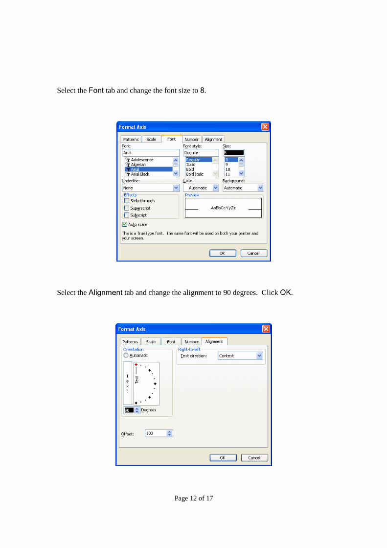
Select the Font tab and change the font size to 8.

Select the Alignment tab and change the alignment to 90 degrees. Click OK.

Page 13 of 17

Your histogram should now look as shown. If you move the mouse arrow over any bar

on the chart, a text box will appear showing the bin label and size of the bar.

For example, moving the arrow over the largest bar shows that 46 data points fall within

the bin range of 18.793 – 18.81.

Histograms are useful in determining if the data is normally distributed. The normal

distribution is easily identifiable by the bell shape of the histogram. You will learn more

about how to identify a normal distribution but for this application, a histogram does an

adequate job of assuring us that the data is normally distributed. Many Quality tools

require that the data be normally distributed in order to be correctly applied.

Save the file to your computer. Ensure that the file is kept in a safe place—backup copies

are encouraged.

Page 14 of 17

You have now completed your initial analysis of the available historical data for Part No.

922. You contacted your supervisor to schedule a meeting to review the findings, and

you were able to show him that the high levels of scrap in the department are most likely

attributable to Rougher 2. He is very pleased with your analysis and quite happy that you

shared the results with the area supervisor who re-targeted Rougher 2 and Rougher 3.

Knowing that you have already impacted the scrap in the department, he is anxious to

support you in taking your investigation further.

He has asked you to put together a slide for the next Operations meeting where he can

share your findings with the plant. He doesn’t want a lot of information, just one page

that shows the capability.

Open Microsoft PowerPoint® and select File, New and Blank Document. Your screen

should look as shown.

Page 15 of 17

In the first text box, type “Capability Study.” In the second text box, type “Rougher 2”

and “Part Number 922.” Reduce the font sizes to around 28 and 18 for the first and

second boxes, respectively.

Open the Excel® file Rougher check sheets.xls and return to Sheet 1 where the

Run chart is located. Click once on the chart to activate it then select Edit, Copy.

Return to PowerPoint® by clicking the mouse on the PowerPoint® icon at the bottom of

your screen.

In PowerPoint® select Edit, Paste Special and then select Picture (Windows

Metafile). Click OK.

Page 16 of 17

A picture of your Run chart will appear. Repeat this process with the histogram. Reduce

the size of the charts and move them off to the right.

Your PowerPoint® file should look generally as shown.

Return to Rougher check sheets.xls, sheet 2, where you generated the

descriptive statistics and calculated the process capability. Paint the range of data that

contains information and select Edit, Copy. Return to PowerPoint® and select Edit,

Paste Special and select Picture (Windows Metafile).

Arrange and size the information so that the slide appears generally as shown.

Page 17 of 17

Save the file as 922 Capability Study.ppt on your computer. Ensure that the

file is kept in a safe place—backup copies are encouraged.