NIST Special Publication 1200-21

Characterization of nanoparticle suspensions

using single particle inductively coupled plasma

mass spectrometry

Version 1.0

K. E. Murphy

J. Liu

A. R. Montoro Bustos

M. E. Johnson

M. R. Winchester

This publication is available free of charge from:

http://dx.doi.org/10.6028/NIST.SP.1200-21

NIST Special Publication 1200-21

Characterization of nanoparticle suspensions

using single particle inductively coupled plasma

mass spectrometry

Version 1.0

K. E. Murphy

A. R. Montoro Bustos

M. E. Johnson

M. R. Winchester Chemical Sciences Division

Material Measurement Laboratory

J. Liu Material Measurement Science Division

Material Measurement Laboratory

This publication is available free of charge from:

http://dx.doi.org/10.6028/NIST.SP.1200-21

December 2015

U.S. Department of Commerce Penny Pritzker, Secretary

National Institute of Standards and Technology

Willie May, Under Secretary of Commerce for Standards and Technology and Director

Certain commercial entities, equipment, or materials may be identified in this

document in order to describe an experimental procedure or concept adequately.

Such identification is not intended to imply recommendation or endorsement by the

National Institute of Standards and Technology, nor is it intended to imply that the

entities, materials, or equipment are necessarily the best available for the purpose.

National Institute of Standards and Technology Special Publication 1200-21

Natl. Inst. Stand. Technol. Spec. Publ. 1200-21, 29 pages (December 2015)

CODEN: NSPUE2

This publication is available free of charge from:

http://dx.doi.org/10.6028/NIST.SP.1200-21

ii

FOREWORD

This National Institute of Standards and Technology (NIST) special publication (SP) is one in a

series of NIST SPs that address research needs articulated in the National Nanotechnology

Initiative (NNI) Environmental, Health, and Safety Research Strategy published in 2011 [1].

This Strategy identified a Nanomaterial Measurement Infrastructure (NMI) as essential for

science-based risk assessment and risk management of nanotechnology-enabled products as

pertaining to human health, exposure, and the environment. NIST was identified as the lead

federal agency in the NMI core research area of the Strategy; this research area includes

measurement tools for the detection and characterization of nanotechnology-enabled products.

Single particle inductively coupled plasma mass spectrometry (spICP-MS) is emerging as a

promising analytical method for the characterization of nanoparticles (NPs) in natural matrices at

environmentally relevant concentrations. The rapid development of spICP-MS for counting and

sizing of NPs has resulted in a wide range of recommended metrological conditions for use in the

implementation of this method.

The objective of this SP is to establish a protocol for the determination of mean nanoparticle size

(equivalent spherical particle diameter), number based size distribution, particle number

concentration and mass concentration of ions in an aqueous suspension of NPs using spICP-MS.

The example presented in this SP pertains to the measurement of gold nanoparticles (AuNPs)

and silver nanoparticles (AgNPs), but the presented protocol is applicable to the measurement of

all spherical nanoparticles containing elements measureable by ICP-MS. In addition, this

protocol describes a Kragten spreadsheet approach for estimation of the expanded uncertainty of

the spICP-MS particle size and particle number concentration measurement.

As the method advances, improvements will be realized and updates to this protocol may be

released in the future. Visit http://www.nist.gov/mml/nanoehs-protocols.cfm to check for

revisions and additions to this protocol or for new protocols in the series. We also encourage

users to report citations to published work in which this protocol has been applied.

1

1. Introduction

Fundamental to the study of environmental and human health effects of engineered

nanomaterials (ENMs) is the ability to characterize the material properties of the ENMs used in

the studies within a dose range and in media commensurate with realistic exposure scenarios.

Many of the traditional methods for characterizing nanoparticles (NPs) do not have the capability

to perform the “in situ” measurements required to establish an accurate assessment of the

potential hazards associated with ENMs. Single particle detection using inductively coupled

plasma mass spectrometry (spICP-MS) is a sensitive and selective method capable of direct

analysis of individual NPs in suspension and which can simultaneously provide information on

size, size distribution, particle number concentration, aggregation state, and ionic content.

2. Principles and Scope

The theoretical basis for spICP-MS was first outlined by Degueldre et al. [2]. Measurements

are performed on commercially available ICP-MS instruments and are acquired in time resolved

mode using short (micro second to millisecond), consecutive, measurement periods referred to as

dwell times (tdwell). spICP-MS relies on the principle that as a NP suspended in a solution is

atomized and ionized in the plasma, it will produce a spatially concentrated packet of ions which

is measured as a transient signal spike superimposed on the steady-state signal produced by any

dissolved analyte. The intensity of the transient signal from a single particle, after subtraction of

the dissolved signal intensity, is proportional to the number of atoms in the particle which can be

converted to element mass and thus diameter to the third power, assuming a spherical particle

shape. The number of pulses counted is proportional to the nanoparticle number concentration.

The intensity of the continuum signal provides a measure of the dissolved metal content. The full

width (at 10 % peak height) of the transient signal from a single particle produced in an ICP-MS

has been measured to be on the order of 0.34 ms [3]. When using dwell times that are

significantly longer than the transient signal from a single particle, it is important that only one

particle is detected per measurement period; coincident particles would result in a bias. Particle

coincidence can be minimized by proper selection of the dwell time and by dilution of the

sample. If a particle event is split between adjacent measurement periods, the intensities in each

measurement period must be summed.

Samples are introduced into the ICP-MS as an aqueous suspension. Only a small

percentage of the sample solution is transported into the plasma. The ratio of the amount of

sample entering the plasma to the amount of sample introduced into the instrument is called the

transport efficiency. Three calibration strategies are currently employed to quantify particle size

and number concentration by spICP-MS: 1) Calibration of the instrument response using

reference nanoparticle standards spanning the linear mass/size range of interest [4]. 2)

Calibration of the instrument response using micro droplet generation [5], and 3) Measurement

of the transport efficiency followed by calibration of the instrument response with ionic standard

solution calibrants [6]. The last calibration strategy in this list is employed in this protocol.

Calibration of the ionic mass fraction concentration is accomplished by measuring ionic standard

solution calibrants.

Detection limits will depend on the elemental composition, the dissolved analyte content,

and the sensitivity of the particular commercial instrument being used. For chemically

homogenous NPs composed of a monoisotopic element (i.e., Au) and containing low mass

2

concentration of ions, diameters in the size range of 10 nm to 200 nm can be measured and

counted, but operating conditions may need to be adjusted to achieve a dynamic size range that is

linear [7].

3. Terminology

Analysis time (t): Total measurement time per sample, e.g. 60 s to 6 min

Dwell time (tdwell): The period during which the detector collects and integrates the

analytical signal (measurement window), e.g. 0.05 ms to 10 ms

Inductively Coupled Plasma Mass Spectrometry (ICP-MS): analytical technique used to

measure the elemental and/or isotopic composition of a sample, based on an instrument

comprising a sample introduction system, an inductively coupled plasma source for

generation of ions of the material(s) under investigation, a plasma/vacuum interface, and a

mass spectrometer comprising an ion focusing, separation and detection system [8].

Matrix: The majority component of a solution.

Nanoparticle: nano-object with all three external dimensions in the nanoscale [9].

Nanoparticle flux (fNP): The number of nanoparticles entering the plasma per unit of time,

e.g., s-1

Nanoparticle number concentration (NP): The number of nanoparticles per volume or mass

of solution, e.g., mL-1

, L-1

, g-1

, kg-1

Transport Efficiency (ηn): ratio of the number of particles or the mass of sample solution

entering the plasma to the number of particles or mass of sample solution introduced into

the instrument

Sample solution flow rate (qliq): The mass or volume of sample solution introduced into the

instrument per unit of time, e.g., g∙min-1

, mL∙min-1

4. Reagents, Materials, and Equipment

4.1 Reagents

4.1.1 De-ionized (DI) water (≥ 18 MΩ·cm resistivity)

Note: To achieve ultra-high purity (UHP) water, the DI feedstock water is

subjected to subboiling distillation in-house.

4.1.2 UHP Nitric Acid, HNO3 (Optima Grade, Fisher Scientific, Pittsburg, PA)

4.1.3 UHP Hydrochloric Acid, HCl (Optima Grade, Fisher Scientific, Pittsburg,

PA)

4.1.4 Thiourea (crystalline, ACS grade, 99 %, Alfa Aesar, Ward Hill, MA)

4.2 Materials

3

4.2.1 Reference Material (RM) 8011 Gold Nanoparticles, Nominal 10 nm Diameter

(NIST, Gaithersburg, MD)

4.2.2 RM 8012 Gold Nanoparticles, Nominal 30 nm Diameter (NIST,

Gaithersburg, MD)

4.2.3 RM 8013 Gold Nanoparticles, Nominal 60 nm Diameter (NIST,

Gaithersburg, MD)

4.2.4 Standard Reference Material (SRM) 3121 Gold (Au) Standard Solution

(NIST, Gaithersburg, MD)

4.2.5 SRM 3151 Silver (Ag) Standard Solution (NIST, Gaithersburg, MD)

4.2.6 RM 8017 PVP-Coated Silver Nanoparticles – Nominal Diameter 75 nm

(NIST, Gaithersburg, MD)

4.3 Labware

4.3.1 Fluorinated Ethylene-Propylene (FEP) or perfluoroalkoxy (PFA) Teflon 1-L

bottles

4.3.2 Nalgene low density polyethylene (LDPE) (30, 60, and 125) mL bottles

4.3.3 Falcon polypropylene 15 mL and 50 mL centrifuge tubes

4.3.4 High density polyethylene (HDPE) 4 mL scintillation vials

4.4 Equipment

4.4.1 ICP-MS capable of tdwell ≤ 10 ms

4.4.2 Analytical balance with readability of 0.1 mg

4.4.3 Ultrasonic bath

5. Reagent Preparation

5.1 Thiourea Diluent for Au standard solution

To improve the chemical stability, stability of the ICP-MS signal profile, and

wash out characteristics of dilute solutions of ionic Au, a diluent composed of 0.5

% mass fraction thiourea, 2.4 % volume fraction HCl, and 0.04 % volume fraction

HNO3 is used. Volume fraction is defined here as the volume of the constituent

divided by the total volume of the solution. The response factor for ionic Au was

tested in the thiourea diluent vs. water and found to be less than 5 % different.

5.1.1 Add 5.00 g of crystalline thiourea to a 1-L, tared, clean PFA or FEP Teflon

bottle followed by 500 g of UHP water. Cap and mix to dissolve the thiourea.

5.1.2 Add 24.00 mL (28.32 g) UHP HCl. Cap and mix.

5.1.3 Add 0.40 mL (0.56 g) UHP HNO3.

5.1.4 Dilute to a final volume of 1.00 L (998.20 g) with UHP water. Cap and mix.

5.2 Dilute HNO3 solution (2 % volume fraction)

Dilute HNO3 solution is used as a rinse between samples during ICP-MS analysis

and in the preparation of dilute ionic silver standard solutions. Improvement in

the chemical stability, stability of the ICP-MS signal profile, and wash out

characteristics for Ag were obtained in dilute acid relative to water alone. On

average, the response factor for ionic Ag in 2 % volume fraction HNO3 solution

was 10 % higher than the response factor for ionic Ag in water though it is

difficult to determine if the observed difference is due to a matrix effect in the

ICP-MS or loss of Ag.

4

5.2.1 Add 40 mL (56.00 g) UHP HNO3 to 1 L UHP water and dilute to 2 L

(1996.40 g) with UHP water.

6. Preparation of Ionic Standard Solution Calibrants

Ionic standard solution calibrants are needed to calibrate the response of the instrument.

The mass fractions given in Tables 1 and 2 serve as a guide and should be adjusted

depending on the sensitivity of the instrument. Mass fractions with resulting count rates

that span the range from 1.0E05 counts per second (cps) to 9.5 E05 cps are

recommended. A balance with a readability of 0.00001 g is used to record the masses for

each of the dilution steps.

6.1 Ionic Au Standard Solution Calibrants

Au standard solution calibrants prepared in thiourea diluent are stable for 1

month.

6.1.1 Au Stock Solution, Dilution 1 (Au Dil1), nominal 1.00E+05 ng/g Au

6.1.1.1 Record the mass of a clean, dry 60 mL LDPE bottle, AuB1

6.1.1.2 Add 0.5 g of SRM 3121 Gold (Au) Standard Solution to the bottle and

record the mass of the bottle + SRM 3121, AuS1.

6.1.1.3 Dilute to 50 g with thiourea diluent and record the mass of the bottle +

SRM 3121 + thiourea diluent, AuD1

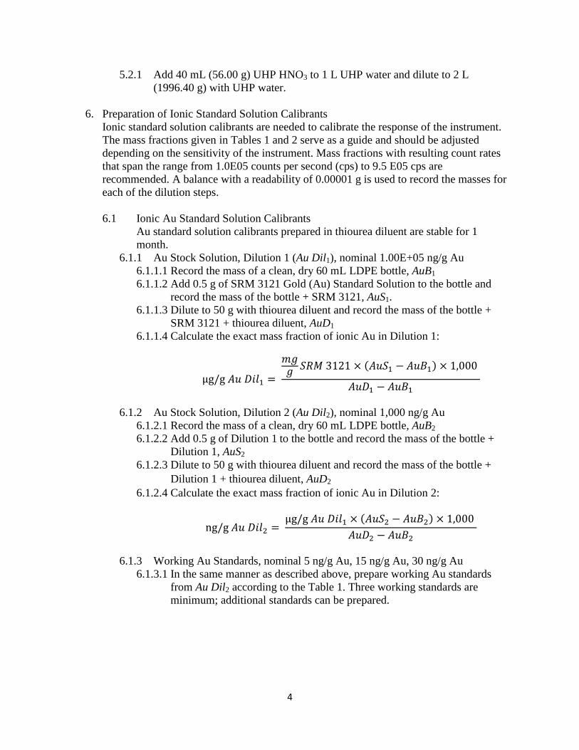
6.1.1.4 Calculate the exact mass fraction of ionic Au in Dilution 1:

µg/g 𝐴𝑢 𝐷𝑖𝑙1 =

𝑚𝑔𝑔 𝑆𝑅𝑀 3121 × (𝐴𝑢𝑆1 − 𝐴𝑢𝐵1) × 1,000

𝐴𝑢𝐷1 − 𝐴𝑢𝐵1

6.1.2 Au Stock Solution, Dilution 2 (Au Dil2), nominal 1,000 ng/g Au

6.1.2.1 Record the mass of a clean, dry 60 mL LDPE bottle, AuB2

6.1.2.2 Add 0.5 g of Dilution 1 to the bottle and record the mass of the bottle +

Dilution 1, AuS2

6.1.2.3 Dilute to 50 g with thiourea diluent and record the mass of the bottle +

Dilution 1 + thiourea diluent, AuD2

6.1.2.4 Calculate the exact mass fraction of ionic Au in Dilution 2:

ng/g 𝐴𝑢 𝐷𝑖𝑙2 = µg/g 𝐴𝑢 𝐷𝑖𝑙1 × (𝐴𝑢𝑆2 − 𝐴𝑢𝐵2) × 1,000

𝐴𝑢𝐷2 − 𝐴𝑢𝐵2

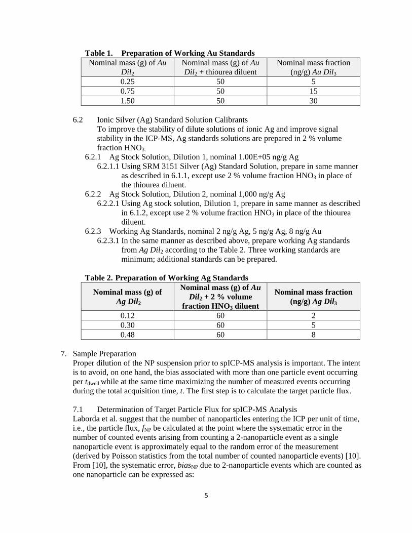
6.1.3 Working Au Standards, nominal 5 ng/g Au, 15 ng/g Au, 30 ng/g Au

6.1.3.1 In the same manner as described above, prepare working Au standards

from Au Dil2 according to the Table 1. Three working standards are

minimum; additional standards can be prepared.

5

Table 1. Preparation of Working Au Standards

Nominal mass (g) of Au

Dil2

Nominal mass (g) of Au

Dil2 + thiourea diluent

Nominal mass fraction

(ng/g) Au Dil3

0.25 50 5

0.75 50 15

1.50 50 30

6.2 Ionic Silver (Ag) Standard Solution Calibrants

To improve the stability of dilute solutions of ionic Ag and improve signal

stability in the ICP-MS, Ag standards solutions are prepared in 2 % volume

fraction HNO3.

6.2.1 Ag Stock Solution, Dilution 1, nominal 1.00E+05 ng/g Ag

6.2.1.1 Using SRM 3151 Silver (Ag) Standard Solution, prepare in same manner

as described in 6.1.1, except use 2 % volume fraction HNO3 in place of

the thiourea diluent.

6.2.2 Ag Stock Solution, Dilution 2, nominal 1,000 ng/g Ag

6.2.2.1 Using Ag stock solution, Dilution 1, prepare in same manner as described

in 6.1.2, except use 2 % volume fraction HNO3 in place of the thiourea

diluent.

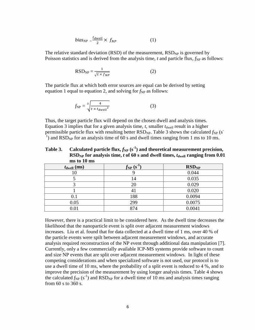
6.2.3 Working Ag Standards, nominal 2 ng/g Ag, 5 ng/g Ag, 8 ng/g Au

6.2.3.1 In the same manner as described above, prepare working Ag standards

from Ag Dil2 according to the Table 2. Three working standards are

minimum; additional standards can be prepared.

Table 2. Preparation of Working Ag Standards

Nominal mass (g) of

Ag Dil2

Nominal mass (g) of Au

Dil2 + 2 % volume

fraction HNO3 diluent

Nominal mass fraction

(ng/g) Ag Dil3

0.12 60 2

0.30 60 5

0.48 60 8

7. Sample Preparation

Proper dilution of the NP suspension prior to spICP-MS analysis is important. The intent

is to avoid, on one hand, the bias associated with more than one particle event occurring

per tdwell while at the same time maximizing the number of measured events occurring

during the total acquisition time, t. The first step is to calculate the target particle flux.

7.1 Determination of Target Particle Flux for spICP-MS Analysis

Laborda et al. suggest that the number of nanoparticles entering the ICP per unit of time,

i.e., the particle flux, fNP be calculated at the point where the systematic error in the

number of counted events arising from counting a 2-nanoparticle event as a single

nanoparticle event is approximately equal to the random error of the measurement

(derived by Poisson statistics from the total number of counted nanoparticle events) [10].

From [10], the systematic error, biasNP due to 2-nanoparticle events which are counted as

one nanoparticle can be expressed as:

6

biasNP ≈ 𝑡𝑑𝑤𝑒𝑙𝑙

2× 𝑓𝑁𝑃 (1)

The relative standard deviation (RSD) of the measurement, RSDNP is governed by

Poisson statistics and is derived from the analysis time, t and particle flux, fNP as follows:

RSDNP = 1

√𝑡 × 𝑓𝑁𝑃 (2)

The particle flux at which both error sources are equal can be derived by setting

equation 1 equal to equation 2, and solving for fNP as follows:

fNP = √4

𝑡 × 𝑡𝑑𝑤𝑒𝑙𝑙2

3 (3)

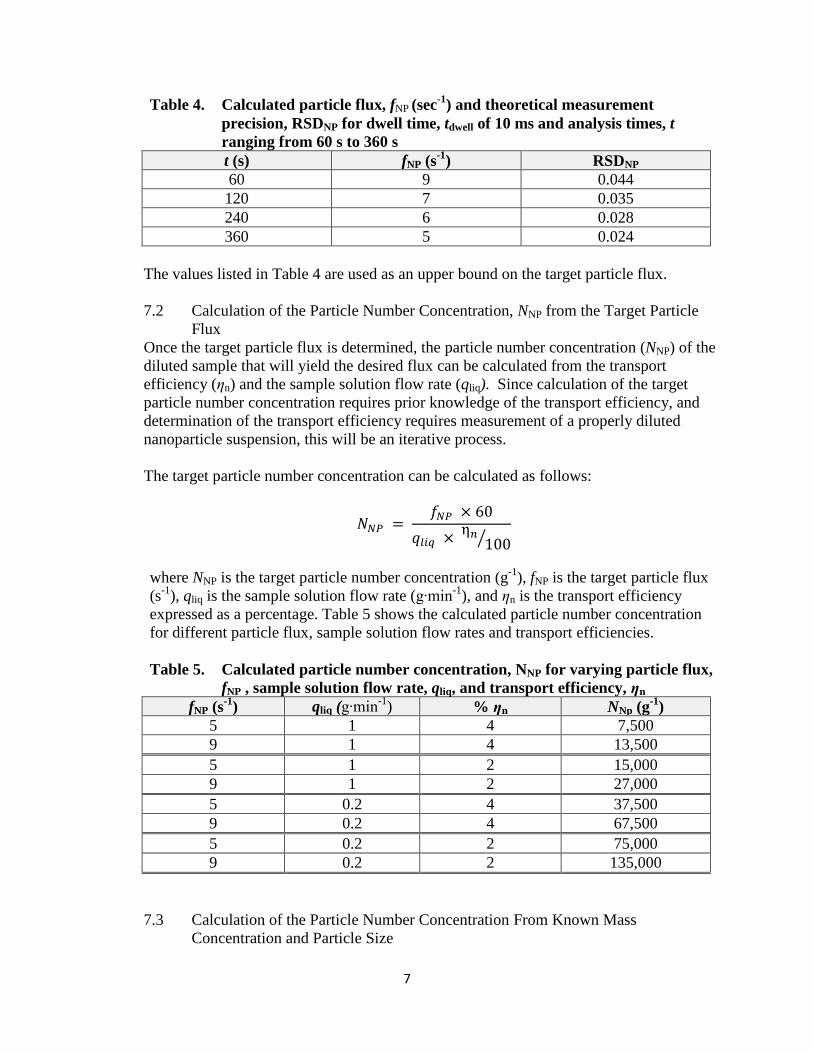
Thus, the target particle flux will depend on the chosen dwell and analysis times.

Equation 3 implies that for a given analysis time, t, smaller tdwell result in a higher

permissible particle flux with resulting better RSDNP. Table 3 shows the calculated fNP (s-

1) and RSDNP for an analysis time of 60 s and dwell times ranging from 1 ms to 10 ms.

Table 3. Calculated particle flux, fNP (s-1

) and theoretical measurement precision,

RSDNP for analysis time, t of 60 s and dwell times, tdwell ranging from 0.01

ms to 10 ms

tdwell (ms) fNP (s-1

) RSDNP

10 9 0.044

5 14 0.035

3 20 0.029

1 41 0.020

0.1 188 0.0094

0.05 299 0.0075

0.01 874 0.0041

However, there is a practical limit to be considered here. As the dwell time decreases the

likelihood that the nanoparticle event is split over adjacent measurement windows

increases. Liu et al. found that for data collected at a dwell time of 1 ms, over 40 % of

the particle events were spilt between adjacent measurement windows, and accurate

analysis required reconstruction of the NP event through additional data manipulation [7].

Currently, only a few commercially available ICP-MS systems provide software to count

and size NP events that are split over adjacent measurement windows. In light of these

competing considerations and when specialized software is not used, our protocol is to

use a dwell time of 10 ms, where the probability of a split event is reduced to 4 %, and to

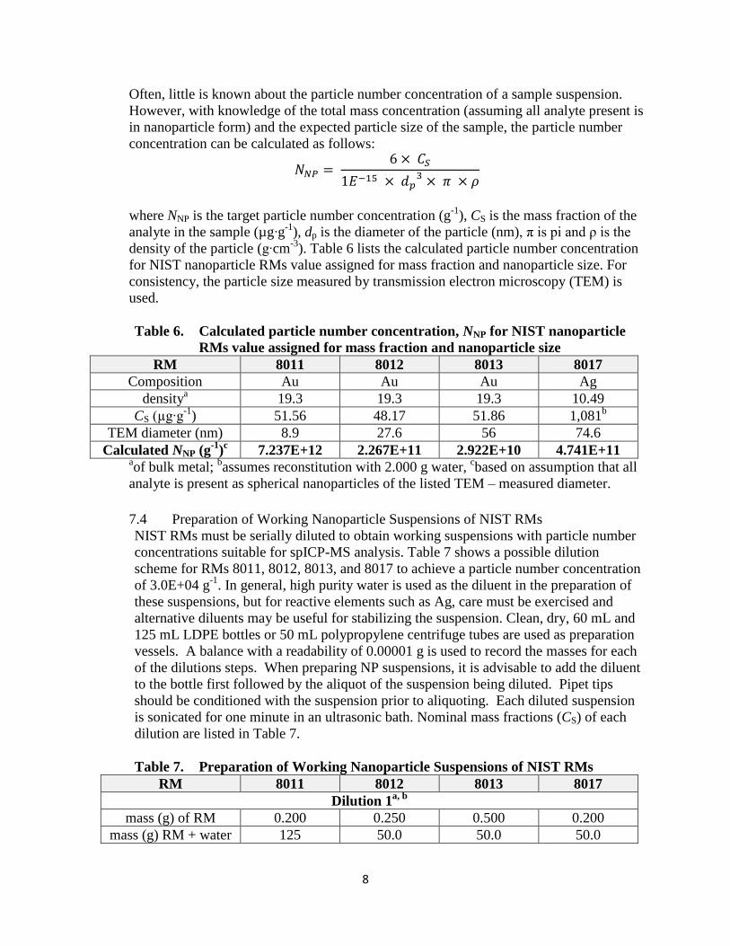
improve the precision of the measurement by using longer analysis times. Table 4 shows

the calculated fNP (s-1

) and RSDNP for a dwell time of 10 ms and analysis times ranging

from 60 s to 360 s.

7

Table 4. Calculated particle flux, fNP (sec-1

) and theoretical measurement

precision, RSDNP for dwell time, tdwell of 10 ms and analysis times, t

ranging from 60 s to 360 s

t (s) fNP (s-1

) RSDNP

60 9 0.044

120 7 0.035

240 6 0.028

360 5 0.024

The values listed in Table 4 are used as an upper bound on the target particle flux.

7.2 Calculation of the Particle Number Concentration, NNP from the Target Particle

Flux

Once the target particle flux is determined, the particle number concentration (NNP) of the

diluted sample that will yield the desired flux can be calculated from the transport

efficiency (ηn) and the sample solution flow rate (qliq). Since calculation of the target

particle number concentration requires prior knowledge of the transport efficiency, and

determination of the transport efficiency requires measurement of a properly diluted

nanoparticle suspension, this will be an iterative process.

The target particle number concentration can be calculated as follows:

𝑁𝑁𝑃 = 𝑓𝑁𝑃 × 60

𝑞𝑙𝑖𝑞 × η𝑛

100⁄

where NNP is the target particle number concentration (g-1

), fNP is the target particle flux

(s-1

), qliq is the sample solution flow rate (g∙min-1

), and ηn is the transport efficiency

expressed as a percentage. Table 5 shows the calculated particle number concentration

for different particle flux, sample solution flow rates and transport efficiencies.

Table 5. Calculated particle number concentration, NNP for varying particle flux,

fNP , sample solution flow rate, qliq, and transport efficiency, ηn

fNP (s-1

) qliq (g∙min-1

) % ηn NNp (g-1

)

5 1 4 7,500

9 1 4 13,500

5 1 2 15,000

9 1 2 27,000

5 0.2 4 37,500

9 0.2 4 67,500

5 0.2 2 75,000

9 0.2 2 135,000

7.3 Calculation of the Particle Number Concentration From Known Mass

Concentration and Particle Size

8

Often, little is known about the particle number concentration of a sample suspension.

However, with knowledge of the total mass concentration (assuming all analyte present is

in nanoparticle form) and the expected particle size of the sample, the particle number

concentration can be calculated as follows:

𝑁𝑁𝑃 = 6 × 𝐶𝑆

1𝐸−15 × 𝑑𝑝3 × 𝜋 × 𝜌

where NNP is the target particle number concentration (g-1

), CS is the mass fraction of the

analyte in the sample (µg∙g-1

), dp is the diameter of the particle (nm), π is pi and ρ is the

density of the particle (g∙cm-3

). Table 6 lists the calculated particle number concentration

for NIST nanoparticle RMs value assigned for mass fraction and nanoparticle size. For

consistency, the particle size measured by transmission electron microscopy (TEM) is

used.

Table 6. Calculated particle number concentration, NNP for NIST nanoparticle

RMs value assigned for mass fraction and nanoparticle size

RM 8011 8012 8013 8017

Composition Au Au Au Ag

densitya 19.3 19.3 19.3 10.49

CS (µg∙g-1

) 51.56 48.17 51.86 1,081b

TEM diameter (nm) 8.9 27.6 56 74.6

Calculated NNP (g-1

)c 7.237E+12 2.267E+11 2.922E+10 4.741E+11

aof bulk metal;

bassumes reconstitution with 2.000 g water,

cbased on assumption that all

analyte is present as spherical nanoparticles of the listed TEM – measured diameter.

7.4 Preparation of Working Nanoparticle Suspensions of NIST RMs

NIST RMs must be serially diluted to obtain working suspensions with particle number

concentrations suitable for spICP-MS analysis. Table 7 shows a possible dilution

scheme for RMs 8011, 8012, 8013, and 8017 to achieve a particle number concentration

of 3.0E+04 g-1

. In general, high purity water is used as the diluent in the preparation of

these suspensions, but for reactive elements such as Ag, care must be exercised and

alternative diluents may be useful for stabilizing the suspension. Clean, dry, 60 mL and

125 mL LDPE bottles or 50 mL polypropylene centrifuge tubes are used as preparation

vessels. A balance with a readability of 0.00001 g is used to record the masses for each

of the dilutions steps. When preparing NP suspensions, it is advisable to add the diluent

to the bottle first followed by the aliquot of the suspension being diluted. Pipet tips

should be conditioned with the suspension prior to aliquoting. Each diluted suspension

is sonicated for one minute in an ultrasonic bath. Nominal mass fractions (CS) of each

dilution are listed in Table 7.

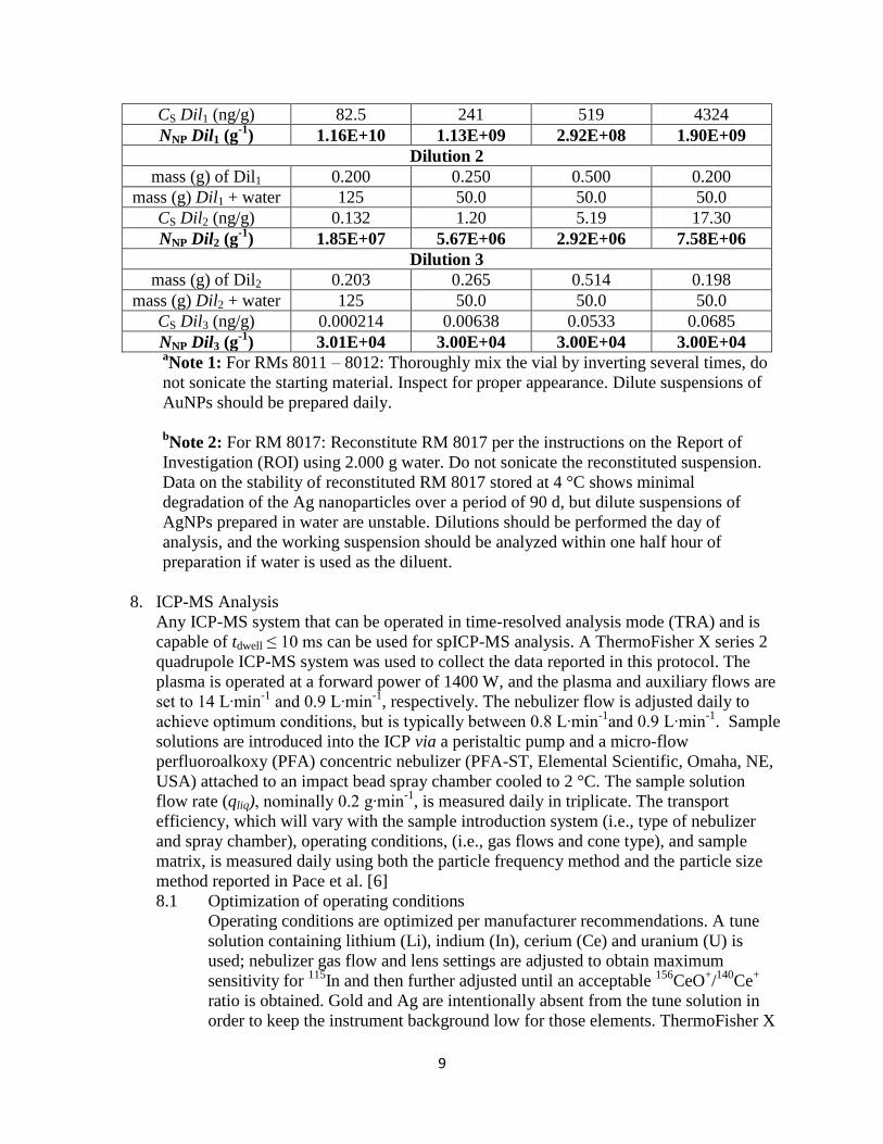
Table 7. Preparation of Working Nanoparticle Suspensions of NIST RMs

RM 8011 8012 8013 8017

Dilution 1a, b

mass (g) of RM 0.200 0.250 0.500 0.200

mass (g) RM + water 125 50.0 50.0 50.0

9

CS Dil1 (ng/g) 82.5 241 519 4324

NNP Dil1 (g-1

) 1.16E+10 1.13E+09 2.92E+08 1.90E+09

Dilution 2

mass (g) of Dil1 0.200 0.250 0.500 0.200

mass (g) Dil1 + water 125 50.0 50.0 50.0

CS Dil2 (ng/g) 0.132 1.20 5.19 17.30

NNP Dil2 (g-1

) 1.85E+07 5.67E+06 2.92E+06 7.58E+06

Dilution 3

mass (g) of Dil2 0.203 0.265 0.514 0.198

mass (g) Dil2 + water 125 50.0 50.0 50.0

CS Dil3 (ng/g) 0.000214 0.00638 0.0533 0.0685

NNP Dil3 (g-1

) 3.01E+04 3.00E+04 3.00E+04 3.00E+04 aNote 1: For RMs 8011 – 8012: Thoroughly mix the vial by inverting several times, do

not sonicate the starting material. Inspect for proper appearance. Dilute suspensions of

AuNPs should be prepared daily.

bNote 2: For RM 8017: Reconstitute RM 8017 per the instructions on the Report of

Investigation (ROI) using 2.000 g water. Do not sonicate the reconstituted suspension.

Data on the stability of reconstituted RM 8017 stored at 4 °C shows minimal

degradation of the Ag nanoparticles over a period of 90 d, but dilute suspensions of

AgNPs prepared in water are unstable. Dilutions should be performed the day of

analysis, and the working suspension should be analyzed within one half hour of

preparation if water is used as the diluent.

8. ICP-MS Analysis

Any ICP-MS system that can be operated in time-resolved analysis mode (TRA) and is

capable of tdwell ≤ 10 ms can be used for spICP-MS analysis. A ThermoFisher X series 2

quadrupole ICP-MS system was used to collect the data reported in this protocol. The

plasma is operated at a forward power of 1400 W, and the plasma and auxiliary flows are

set to 14 L∙min-1

and 0.9 L∙min-1

, respectively. The nebulizer flow is adjusted daily to

achieve optimum conditions, but is typically between 0.8 L∙min-1

and 0.9 L∙min-1

. Sample

solutions are introduced into the ICP via a peristaltic pump and a micro-flow

perfluoroalkoxy (PFA) concentric nebulizer (PFA-ST, Elemental Scientific, Omaha, NE,

USA) attached to an impact bead spray chamber cooled to 2 °C. The sample solution

flow rate (qliq), nominally 0.2 g∙min-1

, is measured daily in triplicate. The transport

efficiency, which will vary with the sample introduction system (i.e., type of nebulizer

and spray chamber), operating conditions, (i.e., gas flows and cone type), and sample

matrix, is measured daily using both the particle frequency method and the particle size

method reported in Pace et al. [6]

8.1 Optimization of operating conditions

Operating conditions are optimized per manufacturer recommendations. A tune

solution containing lithium (Li), indium (In), cerium (Ce) and uranium (U) is

used; nebulizer gas flow and lens settings are adjusted to obtain maximum

sensitivity for 115

In and then further adjusted until an acceptable 156

CeO+/140

Ce+

ratio is obtained. Gold and Ag are intentionally absent from the tune solution in

order to keep the instrument background low for those elements. ThermoFisher X

10

series ICP-MS instruments are supplied with two skimmer cone types, the matrix

tolerant Xt skimmer cone, and the higher sensitivity, Xs cone. The Xs cone

provides the best detection limits; ≥ 700 cps can be obtained for 10 nm AuNPs,

but at the expense of the 156

CeO+/140

Ce+ ratio, which is typically 6 % to 15 % for

the chosen tune conditions. Due to the greater sensitivity for the Xs cones, the

upper size range is limited to about 60 nm AuNPs. Particles larger than this may

exceed the linear dynamic range of the pulse counting detector since the signal

intensity for a spherical particle scales by a power of three relative to the particle

diameter. Though a linear relationship between the pulse stage and analog stage

of the detector can be achieved for ionic standards, our experience with

particulate suspensions is that non- linearity is observed for suspensions

containing large particles whose signal intensity exceeds the range of the pulse

detector. Reducing sensitivity will extend the measureable size range. The Xt

cones are used for routine analysis; conditions are chosen so the 156

CeO+/140

Ce+

ratio is < 2 %, and AuNPs in the range of 20 nm to 80 nm can be measured. The

upper measurable size range can be extended by lowering the signal intensity

using collision cell/kinetic energy discrimination mode or by lowering the

extraction voltage [7]. As the Ag isotopes are half as abundant as the Au isotope,

the lower size limit is 20 nm for AgNPs using the Xs cones, and the upper limit is

100 nm AgNPs with Xt cones under standard conditions. Different ICP-MS

systems will have different lower and upper size detection limits depending on the

sensitivity of the system.

8.2 Analysis Parameters

8.2.1 Au: The 197

Au intensity is recorded in TRA mode using a dwell time of 10 ms

for total analysis times (t) ranging from 100 s to 360 s.

8.2.2 Ag: The 107

Ag intensity is recorded in TRA mode using a dwell time of 10 ms

for total analysis times (t) ranging from 100 s to 360 s.

8.3 Measurement of the Transport Efficiency

Measurement of the transport efficiency via the methods outlined in Pace et al.,

the particle frequency method and the particle size method, requires measurement

of the sample flow, analysis of ionic standards (size method), and analysis of a

standard nanoparticle suspension of known size and mass concentration or

particle number concentration [6] . Calibration of the transport efficiency in this

way means that the overall uncertainty of the spICP-MS measurement of size and

number concentration is directly related to the measurement method and its

associated uncertainty used to value assign the standard nanoparticle suspension.

We use RM 8013 and the size value assigned by TEM, 56 nm ± 0.5 nm. The

derived particle number concentration for RM 8013 is shown in Table 6, and

preparation of the working suspension is described in section 7.4.

Pace et al. reports similar values for the transport efficiency measured using

either the frequency or size method, but we have at times observed that the

transport efficiency measured via the particle frequency method is lower than that

measured by the particle size method. Loss of NPs to the container walls and

pump tubing from the very dilute suspensions required for spICP-MS would

result in a low bias in the transport efficiency measured via the particle frequency

method and could possibly explain at least some of the differences we observe.

11

Tuoriniemi et al. have also identified analyte partitioning effects during

nebulization and off axis trajectories of particles in the plasma as other

considerations that may affect the accurate measurement of the transport

efficiency [11]. Our protocol is to measure the transport efficiency using both

methods (described below), however, our experience has been that when a

difference is observed, the particle size method yields more accurate results.

8.3.1 Measurement and Calculation of sample flow rate, qliq

The sample flow is the amount of sample solution entering the instrument

per unit of time.

8.3.1.1 Measure the total starting mass of the sample solution and its container

using a balance with a readability of 0.0001 g. Record as mstart (g)

8.3.1.2 Using a stop watch, measure the time from when the sample solution

uptake starts to the point where the probe leaves the solution. Record as

tuptake (min)

8.3.1.3 Measure and record the mass of the remaining sample solution and its

container mend (g)

8.3.1.4 Calculate the sample solution flow rate (qliq) as:

sample solution flow rate (𝑔 ∙ 𝑚𝑖𝑛−1) = 𝑚𝑒𝑛𝑑 − 𝑚𝑠𝑡𝑎𝑟𝑡

𝑡𝑢𝑝𝑡𝑎𝑘𝑒

8.3.2 Analysis sequence for the measurement of the transport efficiency

8.3.2.1 Aspirate thiourea solution until instrument background at m/z 197 is at

lowest achievable level.

8.3.2.2 Run samples in the following run sequence: thiourea diluent, water, NP

reference material (i.e., RM 8013 – D-3, see Table 7), working Au

standards from low to high concentration. If desired a second NP reference

material (i.e., RM 8012 – Dil3) can be run and used as an accuracy check.

At least three replicates of the NP reference material are measured and the

results averaged.

8.3.3 Data Analysis

8.3.3.1 Using a spread sheet program such as Microsoft Excel, multiply the data

recorded in counts per second by the dwell time, tdwell, in order to convert

to counts per measurement window.

8.3.3.2 Distinguishing particle events from background

Particle events are distinguished from the background using a n times

standard deviation (n × σ) criterion as described below. Tuoriniemi et al.

suggest that in order to reduce the number of false positives (signals

counted as a particle, but which are not particles) to less than 0.1 % of the

total count, n values larger than 3 must be used. They recommend a value

of n = 5 as a compromise between minimization of the number of false

positives, while not omitting too many particles from being counted that

are in fact particles.

8.3.3.2.1 Order the count data for each sample from largest to smallest

8.3.3.2.2 Compute the mean (µ), standard deviation (σ), and µ + 5 × σ

12

8.3.3.2.3 Using the value for µ + 5 × σ as the cutoff between particle signal

and background, remove the particle signals from the population

and move these data points to a different ‘particle events’ column.

8.3.3.2.4 Compute the mean (µ), standard deviation (σ), and µ + 5 × σ of the

remaining population of data points. If additional particle signals

exceed the new value for µ + 5 × σ, again remove the particle

signals from the population and move these data points to the

‘particle events’ column. Continue this iterative process until none

of the remaining data points exceeds µ + 5 × σ.

8.3.3.2.5 Compute the mean of the data points not considered particle

events, this is the intensity of the dissolved or ionic fraction, Idiss.

Note that this population may also include particles that are too

small to be detected as particles.

8.3.3.2.5.1 Correct Idiss for instrument background by subtracting the mean

of the population of data points measured for the water sample.

8.3.3.3 Split Particle Correction

The transport of particles into the plasma is a random process. It is

possible that a particle event may occur near the end of one measurement

period (dwell time) and spill over into the start of the adjacent

measurement period. This is considered a split particle event. As discussed

in section 7.1, when the chosen dwell time approaches the width of a

single particle event, the likelihood that a particle event is spilt between

adjacent measurement windows increases. For samples of known

monodispersity, as should be the case for the NP standard being used to

measure the transport efficiency, it is possible to correct for split particle

events. Examples of split particle correction for various tdwell are given in

a spreadsheet in the Supporting Information of [7] and will not be

described in detail here. Briefly, the temporal data are examined to locate

occurrences where signal was observed in adjacent measurement

windows. The intensity of the signal in each adjacent measurement

window is compared to the intensity that would be expected for a single

particle event contained completely within one dwell time. If either or

both of the observed intensities in the adjacent measurement windows are

more than 25 % lower than the expected intensity, then the signals are

assumed to be from a single particle event and this split particle event is

corrected by summing the two intensities.

8.3.3.4 Visual inspection for false positives

A false positive is a signal counted as a particle, but which is not a

particle. Though the n times standard deviation (n × σ) criterion described

above is selected to reduce the number of false positives, some false

positives remain in the data set. In situations where the measured

suspension is believed to be monodisperse, contains particles well above

the size detection limit, and contains little or no dissolved analyte, the data

13

set can be visually examined for false positives. In this case, a large gap

(greater than a factor of ten) will exist between the intensity of a true

particle event and false positive events.

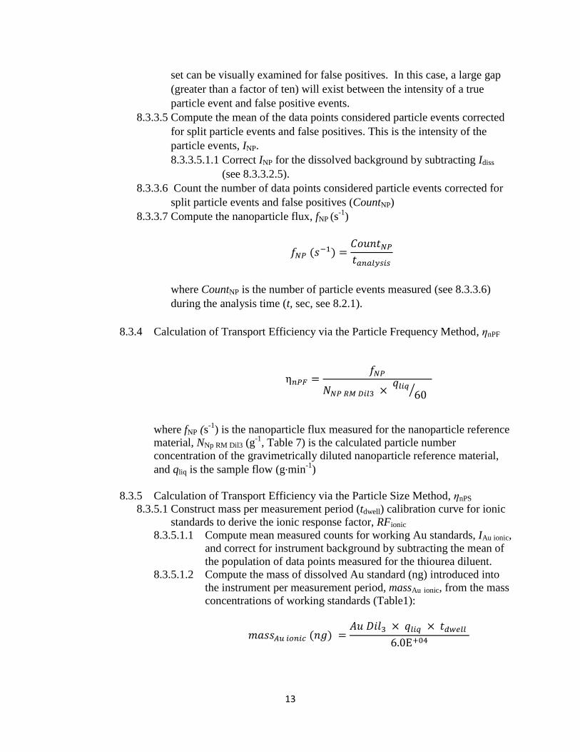
8.3.3.5 Compute the mean of the data points considered particle events corrected

for split particle events and false positives. This is the intensity of the

particle events, INP.

8.3.3.5.1.1 Correct INP for the dissolved background by subtracting Idiss

(see 8.3.3.2.5).

8.3.3.6 Count the number of data points considered particle events corrected for

split particle events and false positives (CountNP)

8.3.3.7 Compute the nanoparticle flux, fNP (s-1

)

𝑓𝑁𝑃 (𝑠−1) =𝐶𝑜𝑢𝑛𝑡𝑁𝑃

𝑡𝑎𝑛𝑎𝑙𝑦𝑠𝑖𝑠

where CountNP is the number of particle events measured (see 8.3.3.6)

during the analysis time (t, sec, see 8.2.1).

8.3.4 Calculation of Transport Efficiency via the Particle Frequency Method, ηnPF

η𝑛𝑃𝐹 =𝑓𝑁𝑃

𝑁𝑁𝑃 𝑅𝑀 𝐷𝑖𝑙3 × 𝑞𝑙𝑖𝑞

60⁄

where fNP (s-1

) is the nanoparticle flux measured for the nanoparticle reference

material, NNp RM Dil3 (g-1

, Table 7) is the calculated particle number

concentration of the gravimetrically diluted nanoparticle reference material,

and qliq is the sample flow (g∙min-1

)

8.3.5 Calculation of Transport Efficiency via the Particle Size Method, ηnPS

8.3.5.1 Construct mass per measurement period (tdwell) calibration curve for ionic

standards to derive the ionic response factor, RFionic

8.3.5.1.1 Compute mean measured counts for working Au standards, IAu ionic,

and correct for instrument background by subtracting the mean of

the population of data points measured for the thiourea diluent.

8.3.5.1.2 Compute the mass of dissolved Au standard (ng) introduced into

the instrument per measurement period, massAu ionic, from the mass

concentrations of working standards (Table1):

𝑚𝑎𝑠𝑠𝐴𝑢 𝑖𝑜𝑛𝑖𝑐 (𝑛𝑔) =𝐴𝑢 𝐷𝑖𝑙3 × 𝑞𝑙𝑖𝑞 × 𝑡𝑑𝑤𝑒𝑙𝑙

6.0E+04

14

where Au Dil3 is the mass fraction of ionic Au in the working

standards (nominal 5 ng/g to 30 ng/g Au), qliq is the sample flow

(g∙min-1

), tdwell is the dwell time (ms).

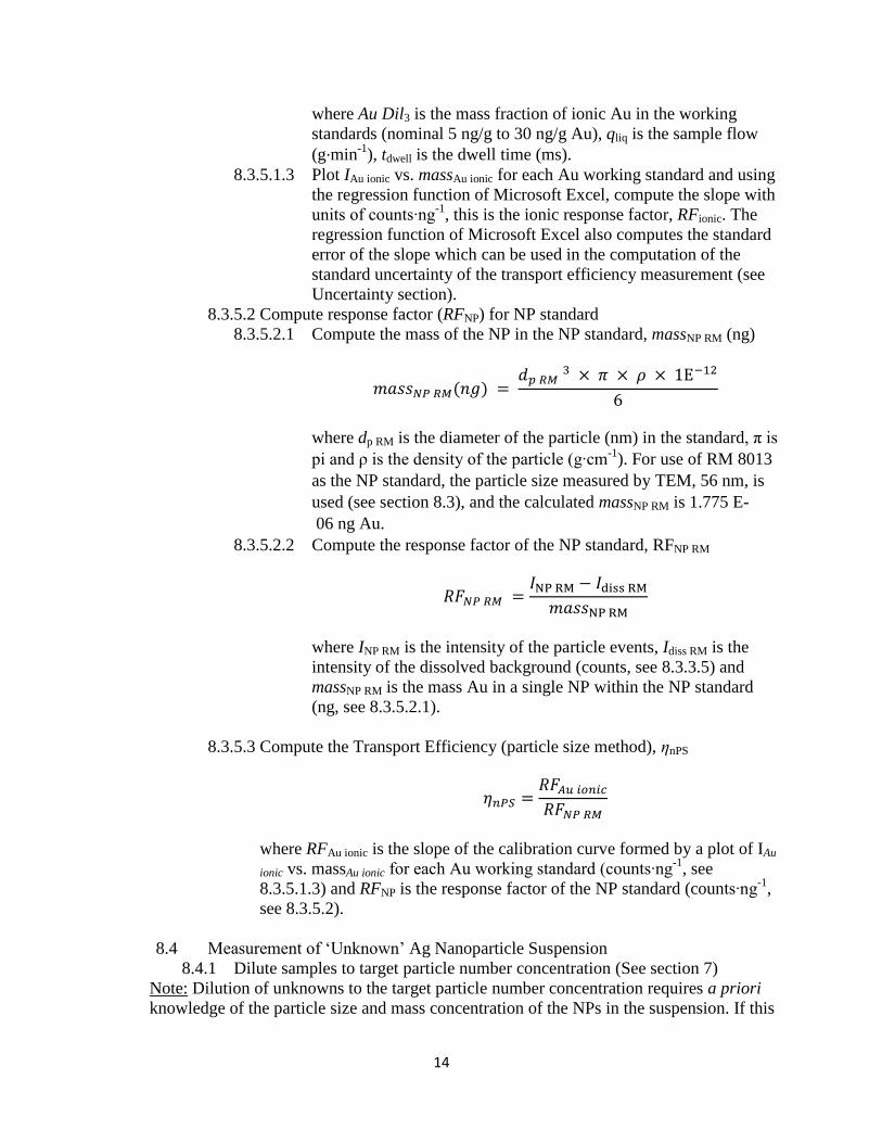
8.3.5.1.3 Plot IAu ionic vs. massAu ionic for each Au working standard and using

the regression function of Microsoft Excel, compute the slope with

units of counts∙ng-1

, this is the ionic response factor, RFionic. The

regression function of Microsoft Excel also computes the standard

error of the slope which can be used in the computation of the

standard uncertainty of the transport efficiency measurement (see

Uncertainty section).

8.3.5.2 Compute response factor (RFNP) for NP standard

8.3.5.2.1 Compute the mass of the NP in the NP standard, massNP RM (ng)

𝑚𝑎𝑠𝑠𝑁𝑃 𝑅𝑀(𝑛𝑔) = 𝑑𝑝 𝑅𝑀 3 × 𝜋 × 𝜌 × 1E−12

6

where dp RM is the diameter of the particle (nm) in the standard, π is

pi and ρ is the density of the particle (g∙cm-1

). For use of RM 8013

as the NP standard, the particle size measured by TEM, 56 nm, is

used (see section 8.3), and the calculated massNP RM is 1.775 E-

06 ng Au.

8.3.5.2.2 Compute the response factor of the NP standard, RFNP RM

𝑅𝐹𝑁𝑃 𝑅𝑀 =𝐼NP RM − 𝐼diss RM

𝑚𝑎𝑠𝑠NP RM

where INP RM is the intensity of the particle events, Idiss RM is the

intensity of the dissolved background (counts, see 8.3.3.5) and

massNP RM is the mass Au in a single NP within the NP standard

(ng, see 8.3.5.2.1).

8.3.5.3 Compute the Transport Efficiency (particle size method), ηnPS

𝜂𝑛𝑃𝑆 =𝑅𝐹𝐴𝑢 𝑖𝑜𝑛𝑖𝑐

𝑅𝐹𝑁𝑃 𝑅𝑀

where RFAu ionic is the slope of the calibration curve formed by a plot of IAu

ionic vs. massAu ionic for each Au working standard (counts∙ng-1

, see

8.3.5.1.3) and RFNP is the response factor of the NP standard (counts∙ng-1

,

see 8.3.5.2).

8.4 Measurement of ‘Unknown’ Ag Nanoparticle Suspension

8.4.1 Dilute samples to target particle number concentration (See section 7)

Note: Dilution of unknowns to the target particle number concentration requires a priori

knowledge of the particle size and mass concentration of the NPs in the suspension. If this

15

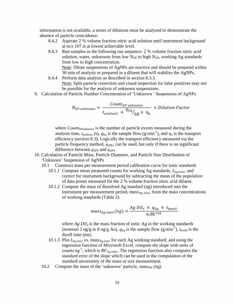
information is not available, a series of dilutions must be analyzed to demonstrate the

absence of particle coincidence.

8.4.2 Aspirate 2 % volume fraction nitric acid solution until instrument background

at m/z 107 is at lowest achievable level.

8.4.3 Run samples in the following run sequence: 2 % volume fraction nitric acid

solution, water, unknowns from low NNP to high NNP, working Ag standards

from low to high concentration.

Note: Dilute suspensions of AgNPs are reactive and should be prepared within

30 min of analysis or prepared in a diluent that will stabilize the AgNPs.

8.4.4 Perform data analysis as described in section 8.3.3.

Note: Split particle correction and visual inspection for false positives may not

be possible for the analysis of unknown suspensions.

9. Calculation of Particle Number Concentration of ‘Unknown ‘ Suspension of AgNPs

𝑁𝑁𝑃 𝑢𝑛𝑘𝑛𝑜𝑤𝑛 = 𝐶𝑜𝑢𝑛𝑡𝑁𝑃 𝑢𝑛𝑘𝑛𝑜𝑤𝑛

𝑡𝑎𝑛𝑎𝑙𝑦𝑠𝑖𝑠 × 𝑞𝑙𝑖𝑞

60⁄ × ηn × 𝐷𝑖𝑙𝑢𝑡𝑖𝑜𝑛 𝐹𝑎𝑐𝑡𝑜𝑟

where CountNPunknown is the number of particle events measured during the

analysis time, tanalysis (s), qliq is the sample flow (g∙min-1

), and ηn is the transport

efficiency (section 8.3). Logically the transport efficiency measured via the

particle frequency method, ηnPF, can be used, but only if there is no significant

difference between ηnPF and ηnPS.

10. Calculation of Particle Mass, Particle Diameter, and Particle Size Distribution of

‘Unknown’ Suspension of AgNPs

10.1 Construct mass per measurement period calibration curve for ionic standards

10.1.1 Compute mean measured counts for working Ag standards, IAg ionic, and

correct for instrument background by subtracting the mean of the population

of data points measured for the 2 % volume fraction nitric acid diluent.

10.1.2 Compute the mass of dissolved Ag standard (ng) introduced into the

instrument per measurement period, massAg ionic, from the mass concentrations

of working standards (Table 2):

𝑚𝑎𝑠𝑠𝐴𝑔 𝑖𝑜𝑛𝑖𝑐(𝑛𝑔) =𝐴𝑔 𝐷𝑖𝑙3 × 𝑞𝑙𝑖𝑞 × 𝑡𝑑𝑤𝑒𝑙𝑙

6.0E+04

where Ag Dil3 is the mass fraction of ionic Ag in the working standards

(nominal 2 ng/g to 8 ng/g Au), qliq is the sample flow (g∙min-1

), tdwell is the

dwell time (ms).

10.1.3 Plot IAg ionic vs. massAg ionic for each Ag working standard, and using the

regression function of Microsoft Excel, compute the slope with units of

counts∙ng-1

, which is RFAg ionic. The regression function also computes the

standard error of the slope which can be used in the computation of the

standard uncertainty of the mass or size measurement.

10.2 Compute the mass of the ‘unknown’ particle, massNP (ng)

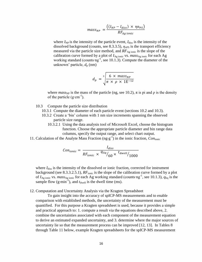
16

𝑚𝑎𝑠𝑠𝑁𝑃 =((𝐼𝑁𝑃 − 𝐼𝑑𝑖𝑠𝑠) × ηn𝑃𝑆)

𝑅𝐹𝐴𝑔 𝑖𝑜𝑛𝑖𝑐

where INP is the intensity of the particle event, Idiss is the intensity of the

dissolved background (counts, see 8.3.3.5), ηnPS is the transport efficiency

measured via the particle size method, and RFAg ionic is the slope of the

calibration curve formed by a plot of IAg ionic vs. massAg ionic for each Ag

working standard (counts∙ng-1

, see 10.1.3). Compute the diameter of the

unknown’ particle, dp (nm)

𝑑𝑝 = √6 × 𝑚𝑎𝑠𝑠𝑁𝑃

𝜋 × 𝜌 × 1E−12

3

where massNP is the mass of the particle (ng, see 10.2), π is pi and ρ is the density

of the particle (g∙cm-1

).

10.3 Compute the particle size distribution

10.3.1 Compute the diameter of each particle event (sections 10.2 and 10.3).

10.3.2 Create a ‘bin’ column with 1 nm size increments spanning the observed

particle size range.

10.3.2.1 Using the data analysis tool of Microsoft Excel, choose the histogram

function. Choose the appropriate particle diameter and bin range data

columns, specify the output range, and select chart output.

11. Calculation of the Analyte Mass Fraction (ng∙g-1) in the ionic fraction, Conionic

𝐶𝑜𝑛𝑖𝑜𝑛𝑖𝑐 = 𝐼𝑑𝑖𝑠𝑠

𝑅𝐹𝑖𝑜𝑛𝑖𝑐 × 𝑞𝑙𝑖𝑞

60⁄ × 𝑡𝑑𝑤𝑒𝑙𝑙

1000⁄

where Idiss is the intensity of the dissolved or ionic fraction, corrected for instrument

background (see 8.3.3.2.5.1), RFionic is the slope of the calibration curve formed by a plot

of IAg ionic vs. massAg ionic for each Ag working standard (counts∙ng-1

, see 10.1.3), qliq is the

sample flow (g∙min-1

), and tdwell is the dwell time (ms).

12. Computation and Uncertainty Analysis via the Kragten Spreadsheet

To gain insight into the accuracy of spICP-MS measurements and to enable

comparison with established methods, the uncertainty of the measurement must be

quantified. For this purpose a Kragten spreadsheet is used, because it provides a simple

and practical approach to: 1. compute a result via the equations described above, 2.

combine the uncertainties associated with each component of the measurement equation

to derive an estimated expanded uncertainty, and 3. determine where the major sources of

uncertainty lie so that the measurement process can be improved [12, 13]. In Tables 8

through Table 11 below, example Kragten spreadsheets for the spICP-MS measurement

17

of transport efficiency via the size and frequency methods, particle number concentration,

and particle size are shown.

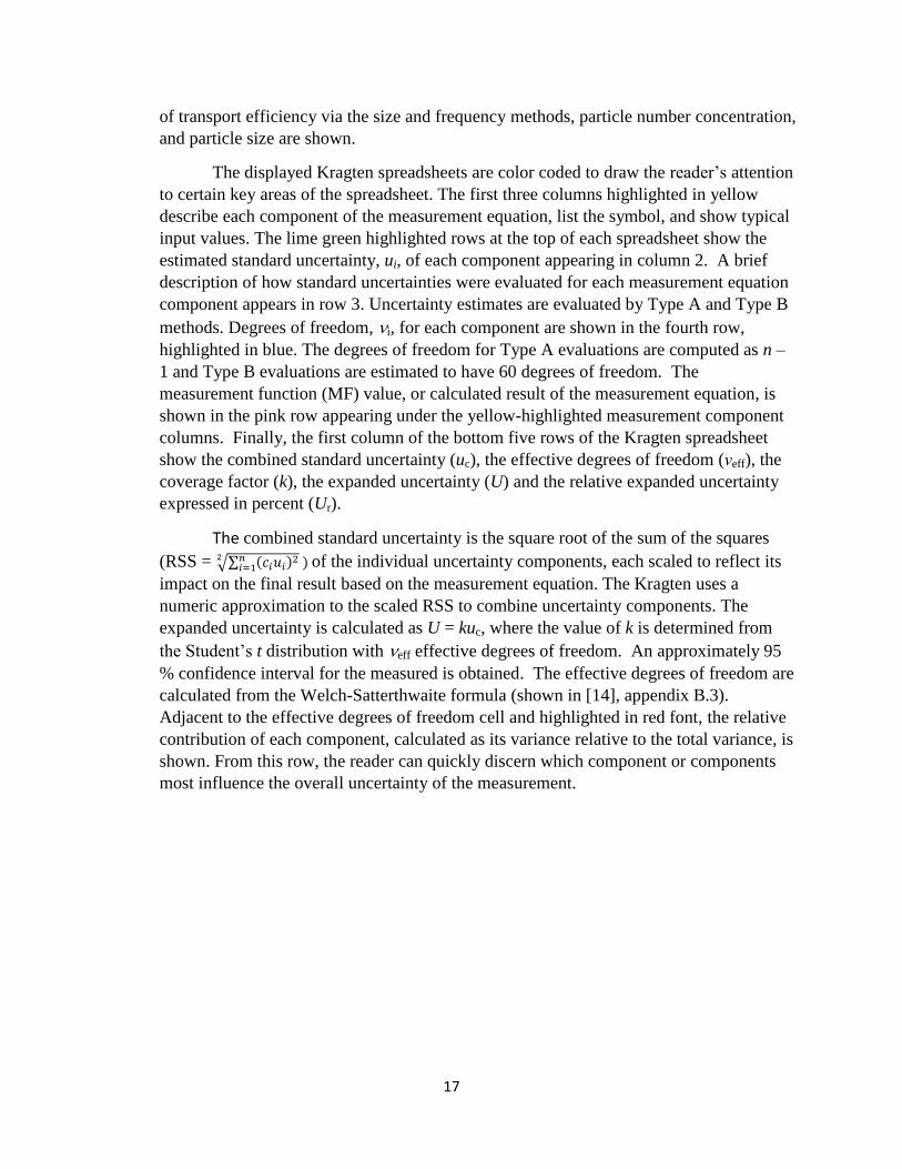
The displayed Kragten spreadsheets are color coded to draw the reader’s attention

to certain key areas of the spreadsheet. The first three columns highlighted in yellow

describe each component of the measurement equation, list the symbol, and show typical

input values. The lime green highlighted rows at the top of each spreadsheet show the

estimated standard uncertainty, ui, of each component appearing in column 2. A brief

description of how standard uncertainties were evaluated for each measurement equation

component appears in row 3. Uncertainty estimates are evaluated by Type A and Type B

methods. Degrees of freedom, i, for each component are shown in the fourth row,

highlighted in blue. The degrees of freedom for Type A evaluations are computed as n –

1 and Type B evaluations are estimated to have 60 degrees of freedom. The

measurement function (MF) value, or calculated result of the measurement equation, is

shown in the pink row appearing under the yellow-highlighted measurement component

columns. Finally, the first column of the bottom five rows of the Kragten spreadsheet

show the combined standard uncertainty (uc), the effective degrees of freedom (νeff), the

coverage factor (k), the expanded uncertainty (U) and the relative expanded uncertainty

expressed in percent (Ur).

The combined standard uncertainty is the square root of the sum of the squares

(RSS = √∑ (𝑐𝑖𝑢𝑖)2𝑛𝑖=1

2 ) of the individual uncertainty components, each scaled to reflect its

impact on the final result based on the measurement equation. The Kragten uses a

numeric approximation to the scaled RSS to combine uncertainty components. The

expanded uncertainty is calculated as U = kuc, where the value of k is determined from

the Student’s t distribution with eff effective degrees of freedom. An approximately 95

% confidence interval for the measured is obtained. The effective degrees of freedom are

calculated from the Welch-Satterthwaite formula (shown in [14], appendix B.3).

Adjacent to the effective degrees of freedom cell and highlighted in red font, the relative

contribution of each component, calculated as its variance relative to the total variance, is

shown. From this row, the reader can quickly discern which component or components

most influence the overall uncertainty of the measurement.

18

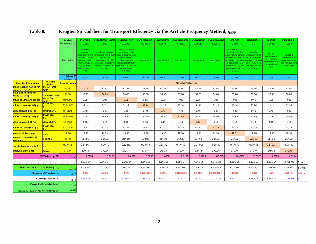
Table 8. Kragten Spreadsheet for Transport Efficiency via the Particle Frequency Method, ηnPF

u(C Au+) u(d RM8013 -TEM) u(aliquot RM) u(Dil. mass, Dil1) u(aliquot Dil1) u(Dil. mass, Dil2) u(aliquot Dil2) u(Dil. mass, Dil3) u(ρ Au) u(CountNP) u(qliq) u(tanalysis)

0.32 0.25 0.00017 0.00017 0.00017 0.00017 0.00017 0.00017 0.010 8.2 0.00091 0.024

Description

combined

standard

uncertainty of the

Au mass fraction

measurement for

RM 8013 AuNPs,

Nominal 60 nm

Diameter from the

ROI

combined standard

uncertainty of the TEM

particle size

measurement for RM

8013 AuNPs, Nominal

60 nm Diameter from

the ROI

estimated standard

uncertainty of the

mass measured on a

5-place analytical

balance from an

assumed rectangular

probability distribution

of magnitude

0.00030 g

see column 6 see column 6 see column 6 see column 6 see column 6

estimated standard

uncertainty for the

density of Au from an

assumed rectangular

probability distribution

of magnitude 0.018

based on variance of

values reported in the

literature.

standard

uncertainty of the

mean measured

number of nominal

60 nm AuNPs for

four replicate runs

of RM 8013

standard

uncertainty of

three replicate

measurements of

the sample flow

rate

standard

uncertainty of the

analysis time for

four replicate runs

of RM 8013

degrees of

freedom i60.00 60.00 60.00 60.00 60.00 60.00 60.00 60.00 60.00 3.0 2.0 3.0

Quantity DescriptionQuantity

Name, Quantity Value

mass fraction Au+ in NP

standard (µg∙g-1

)

C S Au+ RM

801351.86 52.18 51.86 51.86 51.86 51.86 51.86 51.86 51.86 51.86 51.86 51.86 51.86

diameter AuNP in NP

standard (nm) d RM8013 - TEM56.00 56.00 56.25 56.00 56.00 56.00 56.00 56.00 56.00 56.00 56.00 56.00 56.00

mass of NP standard (g)mass RM

80130.04906 0.05 0.05 0.05 0.05 0.05 0.05 0.05 0.05 0.05 0.05 0.05 0.05

dilute to mass (=D-1) (g)Dil. mass,

Dil 131.14147 31.14 31.14 31.14 31.14 31.14 31.14 31.14 31.14 31.14 31.14 31.14 31.14

aliquot mass Dil1 (g) aliquot Dil 1 0.49120 0.49 0.49 0.49 0.49 0.49 0.49 0.49 0.49 0.49 0.49 0.49 0.49

dilute to mass (=D-2) (g)Dil. mass,

Dil 230.95389 30.95 30.95 30.95 30.95 30.95 30.95 30.95 30.95 30.95 30.95 30.95 30.95

aliquot mass Dil2 (g) aliquot Dil 2 1.17502 1.18 1.18 1.18 1.18 1.18 1.18 1.18 1.18 1.18 1.18 1.18 1.18

dilute to Mass (=D-3) (g)Dil. mass,

Dil 361.72538 61.73 61.73 61.73 61.73 61.73 61.73 61.73 61.73 61.73 61.73 61.73 61.73

density of Au (g∙cm-1)ρ Au

19.30 19.30 19.30 19.30 19.30 19.30 19.30 19.30 19.30 19.31 19.30 19.30 19.30

measured number of

particlesCount NP 214.0 214.00 214.00 214.00 214.00 214.00 214.00 214.00 214.00 214.00 222.18 214.00 214.00

sample flow rate (g∙min-1) q liq0.17442 0.17442 0.17442 0.17442 0.17442 0.17442 0.17442 0.17442 0.17442 0.17442 0.17442 0.17533 0.17442

analysis time (sec) t analysis 179.74 179.74 179.74 179.74 179.74 179.74 179.74 179.74 179.74 179.74 179.74 179.74 179.76

MF Value, ηnPF0.0295

0.0293 0.0298 0.0293 0.0295 0.0294 0.0295 0.0294 0.0295 0.0295 0.0306 0.0293 0.0294

-1.81E-04 3.96E-04 -1.04E-04 1.64E-07 -1.04E-05 1.65E-07 -4.34E-06 8.26E-08 1.59E-05 1.13E-03 -1.52E-04 -3.98E-06 c i u i

Combined Standard Uncertainty, u c 0.00123.26E-08 1.57E-07 1.07E-08 2.68E-14 1.08E-10 2.72E-14 1.88E-11 6.83E-15 2.51E-10 1.27E-06 2.31E-08 1.59E-11 (c i u i )

2

Degrees of Freedom, 4.15

2.2% 10.5% 0.7% 0.000002% 0.01% 0.000002% 0.001% 0.0000005% 0.02% 85.0% 1.6% 0.001% rel (c i u i )2

Coverage Factor, k2.78

-5.64E-04 1.58E-03 -5.98E-01 9.46E-04 -5.99E-02 9.51E-04 -2.51E-02 4.77E-04 1.53E-03 1.38E-04 -1.68E-01 -1.64E-04 ci

Expanded Uncertainty, U0.0034

% Relative Expanded Uncertainty U r11.5%

Quantity Value + u i

Standard

Uncertainty, u i

19

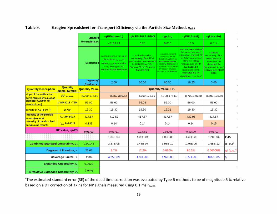
Table 9. Kragten Spreadsheet for Transport Efficiency via the Particle Size Method, ηnPS

aThe estimated standard error (SE) of the dead time correction was evaluated by Type B methods to be of magnitude 5 % relative

based on a DT correction of 37 ns for NP signals measured using 0.1 ms tdwell.

u(RFAu ionic) u(d RM8013 -TEM) u(ρ Au) u(INP AuNP) u(Idiss Au)

43183.93 0.25 0.010 15.5 0.014

Description

standard error of the slope

of the plot of IAu ionic vs.

massAu ionic as computed

using the regression

function of Microsoft Excel

combined standard

uncertainty of the TEM

particle size measurement

for RM 8013 AuNPs,

Nominal 60 nm Diameter

from the ROI

estimated standard

uncertainty for the

density of Au from an

assumed rectangular

probability distribution of

magnitude 0.018 based

on variance of values

reported in the literature.

standard uncertainty of

the mean measured

intensity of nominal 60

nm AuNPs composed

of the SE of four

replicate runs of RM

8013 added in

quadrature to the

estimated SE for

deadtime correctiona

standard

uncertainty of the

mean measured

intensity of the

dissolved Au

background for four

replicate runs of RM

8013

degrees of

freedom i2.00 60.00 60.00 19.25 3.00

Quantity DescriptionQuantity

Name, SymbolQuantity Value

slope of the calibration

curve formed by a plot of RF Au ionic 8,709,175.69 8,752,359.62 8,709,175.69 8,709,175.69 8,709,175.69 8,709,175.69

diameter AuNP in NP

standard (nm)d RM8013 - TEM 56.00 56.00 56.25 56.00 56.00 56.00

density of Au (g∙cm-1) ρ Au 19.30 19.30 19.30 19.31 19.30 19.30

intensity of the particle

events (counts)I NP RM 8013 417.57 417.57 417.57 417.57 433.06 417.57

intensity of the dissolved

background (counts)I diss RM 8013 0.138 0.14 0.14 0.14 0.14 0.15

MF Value, ηnPS0.03703 0.03721 0.03752 0.03705 0.03570 0.03703

1.84E-04 4.98E-04 1.99E-05 -1.33E-03 1.28E-06 c i u i

Combined Standard Uncertainty, u c 0.00143 3.37E-08 2.48E-07 3.98E-10 1.76E-06 1.65E-12 (c i u i )2

Degrees of Freedom, 25.67 1.7% 12.2% 0.020% 86.2% 0.00008% rel (c i u i )2

Coverage Factor, k 2.06 4.25E-09 1.99E-03 1.92E-03 -8.55E-05 8.87E-05 ci

Expanded Uncertainty, U 0.0029

% Relative Expanded Uncertainty U r7.94%

Quantity Value + u i

Standard

Uncertainty, u i

20

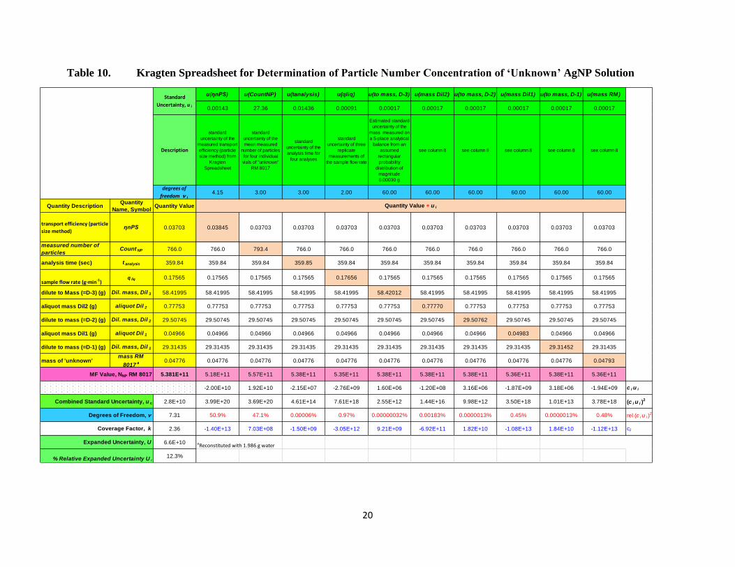
Table 10. Kragten Spreadsheet for Determination of Particle Number Concentration of ‘Unknown’ AgNP Solution

u(ηnPS) u(CountNP) u(tanalysis) u(qliq) u(to mass, D-3) u(mass Dil2) u(to mass, D-2) u(mass Dil1) u(to mass, D-1) u(mass RM)

0.00143 27.36 0.01436 0.00091 0.00017 0.00017 0.00017 0.00017 0.00017 0.00017

Description

standard

uncertainty of the

measured transport

efficiency (particle

size method) from

Kragten

Spreadsheet

standard

uncertainty of the

mean measured

number of particles

for four individual

vials of "unknown"

RM 8017

standard

uncertainty of the

analysis time for

four analyses

standard

uncertainty of three

replicate

measurements of

the sample flow rate

Estimated standard

uncertainty of the

mass measured on

a 5-place analytical

balance from an

assumed

rectangular

probability

distribution of

magnitude

0.00030 g

see column 8 see column 8 see column 8 see column 8 see column 8

degrees of

freedom i4.15 3.00 3.00 2.00 60.00 60.00 60.00 60.00 60.00 60.00

Quantity DescriptionQuantity

Name, SymbolQuantity Value

transport efficiency (particle

size method)ηnPS 0.03703 0.03845 0.03703 0.03703 0.03703 0.03703 0.03703 0.03703 0.03703 0.03703 0.03703

measured number of

particlesCount NP 766.0 766.0 793.4 766.0 766.0 766.0 766.0 766.0 766.0 766.0 766.0

analysis time (sec) t analysis 359.84 359.84 359.84 359.85 359.84 359.84 359.84 359.84 359.84 359.84 359.84

sample flow rate (g∙min-1)q liq 0.17565 0.17565 0.17565 0.17565 0.17656 0.17565 0.17565 0.17565 0.17565 0.17565 0.17565

dilute to Mass (=D-3) (g) Dil. mass, Dil 3 58.41995 58.41995 58.41995 58.41995 58.41995 58.42012 58.41995 58.41995 58.41995 58.41995 58.41995

aliquot mass Dil2 (g) aliquot Dil 2 0.77753 0.77753 0.77753 0.77753 0.77753 0.77753 0.77770 0.77753 0.77753 0.77753 0.77753

dilute to mass (=D-2) (g) Dil. mass, Dil 2 29.50745 29.50745 29.50745 29.50745 29.50745 29.50745 29.50745 29.50762 29.50745 29.50745 29.50745

aliquot mass Dil1 (g) aliquot Dil 1 0.04966 0.04966 0.04966 0.04966 0.04966 0.04966 0.04966 0.04966 0.04983 0.04966 0.04966

dilute to mass (=D-1) (g) Dil. mass, Dil 1 29.31435 29.31435 29.31435 29.31435 29.31435 29.31435 29.31435 29.31435 29.31435 29.31452 29.31435

mass of 'unknown'mass RM

8017a 0.04776 0.04776 0.04776 0.04776 0.04776 0.04776 0.04776 0.04776 0.04776 0.04776 0.04793

MF Value, NNP RM 8017 5.381E+11 5.18E+11 5.57E+11 5.38E+11 5.35E+11 5.38E+11 5.38E+11 5.38E+11 5.36E+11 5.38E+11 5.36E+11

-2.00E+10 1.92E+10 -2.15E+07 -2.76E+09 1.60E+06 -1.20E+08 3.16E+06 -1.87E+09 3.18E+06 -1.94E+09 c i u i

Combined Standard Uncertainty, u c 2.8E+10 3.99E+20 3.69E+20 4.61E+14 7.61E+18 2.55E+12 1.44E+16 9.98E+12 3.50E+18 1.01E+13 3.78E+18 (c i u i )2

Degrees of Freedom, 7.31 50.9% 47.1% 0.00006% 0.97% 0.00000032% 0.00183% 0.0000013% 0.45% 0.0000013% 0.48% rel (c i u i )2

Coverage Factor, k 2.36 -1.40E+13 7.03E+08 -1.50E+09 -3.05E+12 9.21E+09 -6.92E+11 1.82E+10 -1.08E+13 1.84E+10 -1.12E+13 ci

Expanded Uncertainty, U 6.6E+10 aReconstituted with 1.986 g water

% Relative Expanded Uncertainty U r12.3%

Quantity Value + u i

Standard

Uncertainty, u i

21

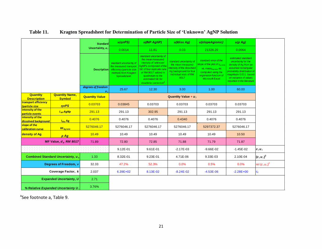
Table 11. Kragten Spreadsheet for Determination of Particle Size of ‘Unknown’ AgNP Solution

aSee footnote a, Table 9.

u(ηnPS) u(INP AgNP) u(Idiss Ag) u(slopeAgionic) u(ρ Ag)

0.0014 11.81 0.03 21326.20 0.0064

Description

standard uncertainty of

the measured transport

efficiency (particle size

method) from Kragten

Spreadsheet

standard uncertainty of

the mean measured

intensity of 'unknown'

AgNPs composed of the

SE of four replicate runs

of RM 8017 added in

quadrature to the

estimated SE for

deadtime correctiona

standard uncertainty of

the mean measured

intensity of the dissolved

Ag background for four

individual vials of RM

8017

standard error of the

slope of the plot of IAg ionic

vs. massAg ionic as

computed using the

regression function of

Microsoft Excel

estimated standard

uncertainty for the

density of Ag from an

assumed rectangular

probability distribution of

magnitude 0.011 based

on variance of values

reported in the literature

degrees of freedom

i25.67 12.30 3.00 1.00 60.00

Quantity

Description

Quantity Name,

SymbolQuantity Value

transport efficiency

(particle size ηnPS0.03703 0.03845 0.03703 0.03703 0.03703 0.03703

intensity of the

particle events I NP AgNp 291.13 291.13 302.95 291.13 291.13 291.13

intensity of the

dissolved background Idiss Ag 0.4076 0.4076 0.4076 0.4340 0.4076 0.4076

slope of the

calibration curve RFAg ionic5276046.17 5276046.17 5276046.17 5276046.17 5297372.37 5276046.17

density of Agρ Ag

10.49 10.49 10.49 10.49 10.49 10.50

MF Value, d p RM 8017 71.89 72.80 72.85 71.88 71.79 71.87

9.12E-01 9.61E-01 -2.17E-03 -9.66E-02 -1.45E-02 c i u i

Combined Standard Uncertainty, u c 1.33 8.32E-01 9.23E-01 4.71E-06 9.33E-03 2.10E-04 (c i u i )2

Degrees of Freedom, 32.33 47.2% 52.3% 0.0% 0.5% 0.0% rel (c i u i )2

Coverage Factor, k 2.037 6.39E+02 8.13E-02 -8.24E-02 -4.53E-06 -2.28E+00 ci

Expanded Uncertainty, U 2.71

% Relative Expanded Uncertainty U r3.76%

Quantity Value + u i

Standard

Uncertainty, u i

22

13. Outcomes

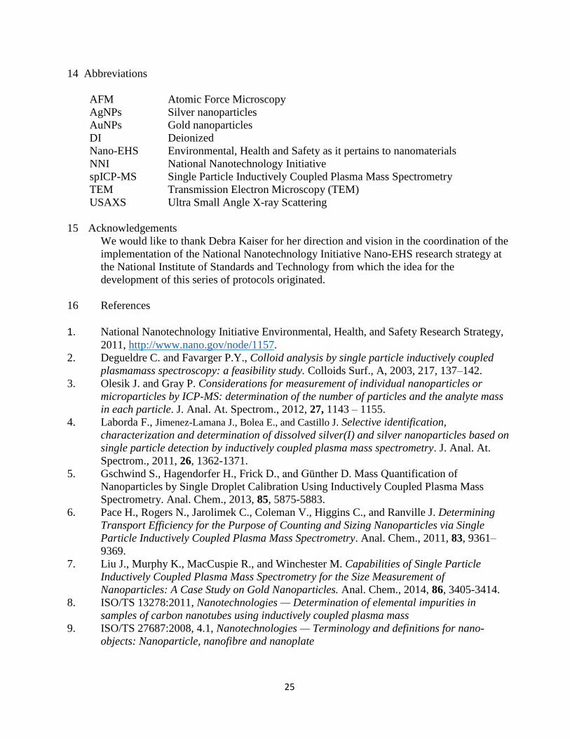
13.1 spICP-MS time resolved intensity profile and particle size distribution of RM 8017

PVP-Coated Silver Nanoparticles – Nominal Core Diameter 75 nm

A typical time-resolved spICP-MS intensity profile and corresponding particle

size distribution for a dilute suspension of a single vial of RM 8017 are shown in

Figure 1. After reconstitution of the RM per instructions on the report of

investigation (ROI), the suspension was diluted with water 28-million fold (see

section 7.4) to a nominal particle number concentration of 1.7E04 g

-1, and measured

within 0.5 h of dilution. The intensity of each signal pulse is proportional to the

mass of analyte in a particle, and by assumption of a spherical shape, particle

diameter. The number of signal pulses is proportional to the particle number

concentration.

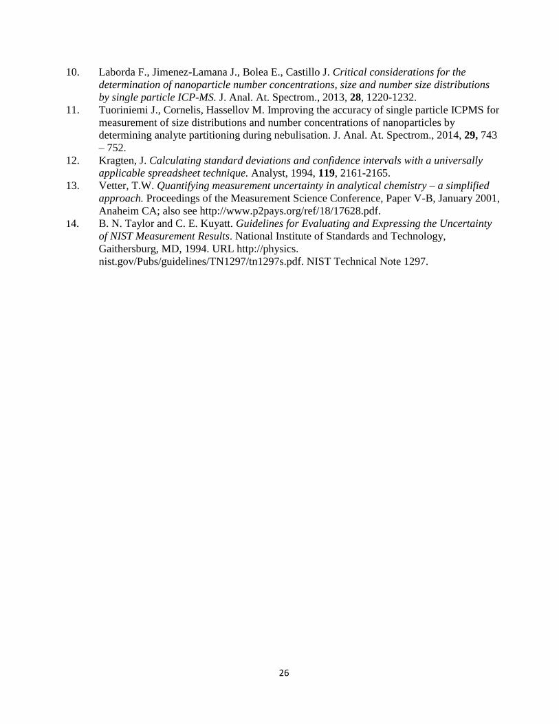
Ionic silver (Ag+), if present in the sample suspension, can be observed in a

spICP-MS time intensity profile as steady-state signal at the base of the signal

pulses formed by particles. An example is shown in Figure 2, which shows spICP-

MS results for a dilute AgNP suspension (2.5E04 g-1

, RM 8017) stored for 24 h at

room temperature. The instability of the AgNP suspension under these storage

conditions is evidenced by a smaller measured particle size, reduced particle

number concentration, and an increased mass fraction of ionic Ag.

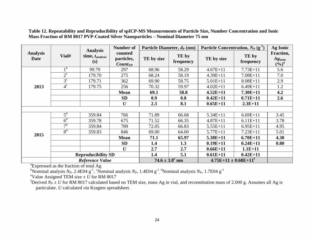
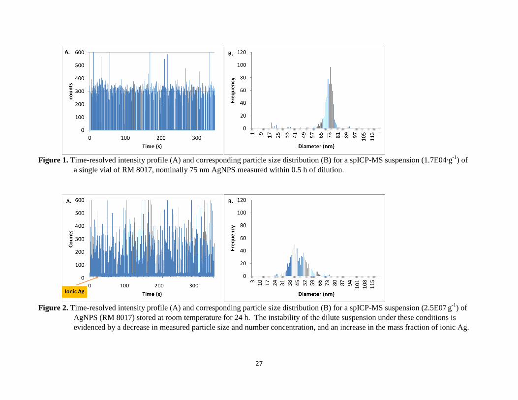
13.2 Repeatability, reproducibility and comparability of spICP-MS Measurements

Results for the spICP-MS measurement of particle size, number

concentration and ionic mass fraction in eight vials of RM 8017 that demonstrate

the repeatability and reproducibility of the method are presented in Table 12. The

comparability of the spICP-MS particle size results with mean particle sizes

measured by TEM, atomic force microscopy (AFM), and ultra-small angle X-ray

scattering (USAXS) is illustrated in Figure 3. The comparability of spICP-MS

number concentration results with a derived number concentration value for RM

8017 is shown in Figure 4.

The spICP-MS measurements were performed in separate experiments (four

vials per experiment), conducted two years apart, and the presented results are

calculated using both the size and frequency based measure of transport efficiency.

Under repeatability conditions, a standard deviation of no greater than ± 1.4 nm

was observed for the nominally 75 nm AgNPs. Reproducibility conditions yielded

a similar standard deviation for the results using the size based measure of

transport efficiency, but results calculated using the frequency based measure of

transport efficiency showed a larger standard deviation (± 5.1 nm). The estimated

expanded uncertainty of the size measurement (see section 12.0 and example

Kragten spreadsheet in Table 11) ranged from ± 2.3 nm (3 % relative) using the

particle size-based measure of transport efficiency to ± 8.1 nm (± 14 % relative)

using the frequency-based measure of transport efficiency. The plot in Figure 3

shows that the particle size calculated using the frequency-based measure of

23

transport efficiency yields results that are lower than results using the size-based

measure of transport efficiency and in addition, are lower than the TEM value.

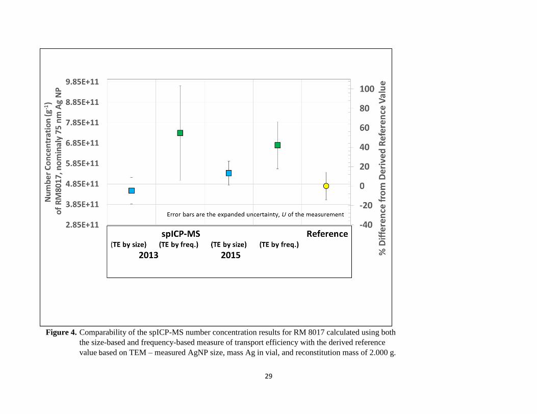
spICP-MS measured number concentration results show greater variability

and poorer comparability than the spICP-MS size measurements (see Table 12 and

Figure 4). Under repeatability conditions, standard deviations ranged from

± 1.9E10 g-1

(4 % relative) to ± 7.1E10 g-1

(10 % relative). Standard deviations

under reproducibility conditions were similar. Here again, differences in the results

calculated using the two measures of transport efficiency are observed, with the

frequency-based measure yielding results that deviated farthest from the reference

value. The reference value for RM 8017 was computed from the TEM measured

particle size, the value assigned mass of Ag in the vial, and assuming a

reconstitution mass of 2.000 g. Measured spICP-MS number concentrations using

the size-based measure of transport efficiency were in good agreement with the

computed number concentration reference value for RM 8017; however the

measured spICP-MS number concentrations using the frequency-based measure of

transport efficiency were biased high by 42 % to 55 %. This indicates that the

frequency-based measurement of transport efficiency is biased low, presumably

due to loss of AuNPs. Analysis of the total Au mass fraction via acid digestion of

a spICP-MS suspension diluted to 1.6E4 g-1

that was used to measure transport

efficiency did show that the measured Au mass fraction was significantly lower

than expected, indicating loss of Au to the container walls. A more rigorous study

of the stability of the very dilute suspension required for spICP-MS measurements

with respect to particle number concentration, is needed. It is worthy to note that

the size-based measurement of transport efficiency is more robust, as it is

unaffected by particle loss to the container walls.

The Ag ion content measured in each vial of RM 8017 and expressed as the

fraction of total Ag is listed in the last column of Table 12. It should be noted that

RM 8017 is not an ideal sample for measurement of the component Ag ion

content. Since RM 8017 is a freeze-dried material that is designed to be

reconstituted and used within as short time frame, a reference value for the Ag ion

content of RM 8017 has not been established. Furthermore due to the high AgNP

concentration and subsequent large dilution (nominally 28 million-fold) required to

achieve the optimum number concentration for single particle analysis, the ionic

Ag content, if any, has been so diluted that the measured signals are at the method

detection limit and subject to high uncertainty. This is evident in the observed

variability of the results. Measurement of the ionic fraction of a less concentrated

solution with respect to particle number, would presumably yield more consistent

results.

24

Table 12. Repeatability and Reproducibility of spICP-MS Measurements of Particle Size, Number Concentration and Ionic

Mass Fraction of RM 8017 PVP-Coated Silver Nanoparticles – Nominal Diameter 75 nm

Analysis

Date Vial#

Analysis

time, tanalysis

(s)

Number of

counted

particles,

CountNP

Particle Diameter, dP (nm) Particle Concentration, NP (g-1

) Ag Ionic

Fraction,

Agionic

(%)a

TE by size TE by

frequency TE by size

TE by

frequency

2013

1b 99.79 297 68.96 58.29 4.67E+11 7.73E+11 5.6

2c 179.70 275 68.24 58.19 4.39E+11 7.08E+11 7.0

3c 179.71 362 69.90 58.75 5.01E+11 8.08E+11 2.9

4c 179.75 256 70.32 59.97 4.02E+11 6.49E+11 1.2

Mean 69.1 58.8 4.52E+11 7.30E+11 4.2

SD 0.9 0.8 0.42E+11 0.71E+11 2.6

U 2.3 8.1 0.65E+11 2.3E+11

2015

5d 359.84 766 71.89 66.68 5.34E+11 6.69E+11 3.45

6d 359.78 675 71.52 66.35 4.87E+11 6.11E+11 3.78

7d 359.84 789 72.05 66.83 5.55E+11 6.95E+11 4.95

8d 359.83 846 69.00 64.00 5.77E+11 7.23E+11 5.01

Mean 71.1 65.97 5.38E+11 6.70E+11 4.30

SD 1.4 1.3 0.19E+11 0.24E+11 0.80

U 2.7 2.7 0.66E+11 1.1E+11

Reproducibility SD 1.4 5.1 0.61E+11 0.42E+11

Reference Value 74.6 ± 3.8e nm 4.75E+11 ± 0.68E+11

f

aExpressed as the fraction of total Ag

bNominal analysis NP, 2.4E04 g

-1,

cNominal analysis NP, 1.4E04 g

-1, dNominal analysis NP, 1.7E04 g

-1

eValue Assigned TEM size ± U for RM 8017

fDerived NP ± U for RM 8017 calculated based on TEM size, mass Ag in vial, and reconstitution mass of 2.000 g. Assumes all Ag is

particulate. U calculated via Kragten spreadsheet.

25

14 Abbreviations

AFM Atomic Force Microscopy

AgNPs Silver nanoparticles

AuNPs Gold nanoparticles

DI Deionized

Nano-EHS Environmental, Health and Safety as it pertains to nanomaterials

NNI National Nanotechnology Initiative

spICP-MS Single Particle Inductively Coupled Plasma Mass Spectrometry

TEM Transmission Electron Microscopy (TEM)

USAXS Ultra Small Angle X-ray Scattering

15 Acknowledgements

We would like to thank Debra Kaiser for her direction and vision in the coordination of the

implementation of the National Nanotechnology Initiative Nano-EHS research strategy at

the National Institute of Standards and Technology from which the idea for the

development of this series of protocols originated.

16 References

1. National Nanotechnology Initiative Environmental, Health, and Safety Research Strategy,

2011, http://www.nano.gov/node/1157.

2. Degueldre C. and Favarger P.Y., Colloid analysis by single particle inductively coupled

plasmamass spectroscopy: a feasibility study. Colloids Surf., A, 2003, 217, 137–142.

3. Olesik J. and Gray P. Considerations for measurement of individual nanoparticles or

microparticles by ICP-MS: determination of the number of particles and the analyte mass

in each particle. J. Anal. At. Spectrom., 2012, 27, 1143 – 1155.

4. Laborda F., Jimenez-Lamana J., Bolea E., and Castillo J. Selective identification,

characterization and determination of dissolved silver(I) and silver nanoparticles based on

single particle detection by inductively coupled plasma mass spectrometry. J. Anal. At.

Spectrom., 2011, 26, 1362-1371.

5. Gschwind S., Hagendorfer H., Frick D., and Gunther D. Mass Quantification of

Nanoparticles by Single Droplet Calibration Using Inductively Coupled Plasma Mass

Spectrometry. Anal. Chem., 2013, 85, 5875-5883.

6. Pace H., Rogers N., Jarolimek C., Coleman V., Higgins C., and Ranville J. Determining

Transport Efficiency for the Purpose of Counting and Sizing Nanoparticles via Single

Particle Inductively Coupled Plasma Mass Spectrometry. Anal. Chem., 2011, 83, 9361–

9369.

7. Liu J., Murphy K., MacCuspie R., and Winchester M. Capabilities of Single Particle

Inductively Coupled Plasma Mass Spectrometry for the Size Measurement of

Nanoparticles: A Case Study on Gold Nanoparticles. Anal. Chem., 2014, 86, 3405-3414.

8. ISO/TS 13278:2011, Nanotechnologies — Determination of elemental impurities in

samples of carbon nanotubes using inductively coupled plasma mass

9. ISO/TS 27687:2008, 4.1, Nanotechnologies — Terminology and definitions for nano-

objects: Nanoparticle, nanofibre and nanoplate

26

10. Laborda F., Jimenez-Lamana J., Bolea E., Castillo J. Critical considerations for the

determination of nanoparticle number concentrations, size and number size distributions

by single particle ICP-MS. J. Anal. At. Spectrom., 2013, 28, 1220-1232.

11. Tuoriniemi J., Cornelis, Hassellov M. Improving the accuracy of single particle ICPMS for

measurement of size distributions and number concentrations of nanoparticles by

determining analyte partitioning during nebulisation. J. Anal. At. Spectrom., 2014, 29, 743

– 752.

12. Kragten, J. Calculating standard deviations and confidence intervals with a universally

applicable spreadsheet technique. Analyst, 1994, 119, 2161-2165.

13. Vetter, T.W. Quantifying measurement uncertainty in analytical chemistry – a simplified

approach. Proceedings of the Measurement Science Conference, Paper V-B, January 2001,

Anaheim CA; also see http://www.p2pays.org/ref/18/17628.pdf.

14. B. N. Taylor and C. E. Kuyatt. Guidelines for Evaluating and Expressing the Uncertainty

of NIST Measurement Results. National Institute of Standards and Technology,

Gaithersburg, MD, 1994. URL http://physics.

nist.gov/Pubs/guidelines/TN1297/tn1297s.pdf. NIST Technical Note 1297.

27

Figure 1. Time-resolved intensity profile (A) and corresponding particle size distribution (B) for a spICP-MS suspension (1.7E04∙g

-1) of

a single vial of RM 8017, nominally 75 nm AgNPS measured within 0.5 h of dilution.

Figure 2. Time-resolved intensity profile (A) and corresponding particle size distribution (B) for a spICP-MS suspension (2.5E07

g

-1) of

AgNPS (RM 8017) stored at room temperature for 24 h. The instability of the dilute suspension under these conditions is

evidenced by a decrease in measured particle size and number concentration, and an increase in the mass fraction of ionic Ag.

28

Figure 3. Comparability of the spICP-MS particle size results for RM 8017 calculated using both the size-based

and frequency-based measure of transport efficiency with mean particle sizes measured by TEM, AFM,

and USAXS

29

Figure 4. Comparability of the spICP-MS number concentration results for RM 8017 calculated using both

the size-based and frequency-based measure of transport efficiency with the derived reference

value based on TEM – measured AgNP size, mass Ag in vial, and reconstitution mass of 2.000 g.