Embed Size (px)
Citation preview
Fishery Data Series No. 18-13
Chinook Salmon Escapement in the Chena and Salcha Rivers and Coho Salmon Escapement in the Delta Clearwater River, 2016
by
Lisa Stuby
and
Matt Tyers
July 2018
Alaska Department of Fish and Game Divisions of Sport Fish and Commercial Fisheries
Symbols and Abbreviations The following symbols and abbreviations, and others approved for the Système International d'Unités (SI), are used without definition in the following reports by the Divisions of Sport Fish and of Commercial Fisheries: Fishery Manuscripts, Fishery Data Series Reports, Fishery Management Reports, and Special Publications. All others, including deviations from definitions listed below, are noted in the text at first mention, as well as in the titles or footnotes of tables, and in figure or figure captions. Weights and measures (metric) centimeter cm deciliter dL gram g hectare ha kilogram kg kilometer km liter L meter m milliliter mL millimeter mm
Weights and measures (English) cubic feet per second ft3/s foot ft gallon gal inch in mile mi nautical mile nmi ounce oz pound lb quart qt yard yd
Time and temperature day d degrees Celsius °C degrees Fahrenheit °F degrees kelvin K hour h minute min second s
Physics and chemistry all atomic symbols alternating current AC ampere A calorie cal direct current DC hertz Hz horsepower hp hydrogen ion activity pH (negative log of) parts per million ppm parts per thousand ppt,
‰ volts V watts W
General Alaska Administrative Code AAC all commonly accepted abbreviations e.g., Mr., Mrs.,
AM, PM, etc. all commonly accepted professional titles e.g., Dr., Ph.D.,
R.N., etc. at @ compass directions:
east E north N south S west W
copyright corporate suffixes:
Company Co. Corporation Corp. Incorporated Inc. Limited Ltd.
District of Columbia D.C. et alii (and others) et al.et cetera (and so forth) etc. exempli gratia (for example) e.g.Federal Information Code FIC id est (that is) i.e. latitude or longitude lat or long monetary symbols (U.S.) $, ¢ months (tables and
figures): first three letters Jan,...,Dec registered trademark trademark United States (adjective) U.S. United States of America (noun) USA U.S.C. United States
Code U.S. state use two-letter
abbreviations (e.g., AK, WA)
Mathematics, statistics all standard mathematical signs, symbols and abbreviations alternate hypothesis HA base of natural logarithm e catch per unit effort CPUE coefficient of variation CV common test statistics (F, t, χ2, etc.) confidence interval CI correlation coefficient (multiple) R
correlation coefficient (simple) r covariance cov degree (angular) ° degrees of freedom df expected value E greater than > greater than or equal to ≥ harvest per unit effort HPUE less than < less than or equal to ≤ logarithm (natural) ln logarithm (base 10) log logarithm (specify base) log2, etc. minute (angular) ' not significant NS null hypothesis HO percent % probability P probability of a type I error (rejection of the null
hypothesis when true) α probability of a type II error (acceptance of the null
hypothesis when false) β second (angular) " standard deviation SD standard error SE variance population Var sample var
FISHERY DATA SERIES NO. 18-13
CHINOOK SALMON ESCAPEMENT IN THE CHENA AND SALCHA RIVERS AND COHO SALMON ESCAPEMENT IN THE DELTA
CLEARWATER RIVER, 2016
by Lisa Stuby
and Matt Tyers
Division of Sport Fish, Fairbanks
Alaska Department of Fish and Game Division of Sport Fish, Research and Technical Services 333 Raspberry Road, Anchorage, Alaska, 99518-1599
July 2018
Development and publication of this manuscript were partially financed by the Federal Aid in Sport fish Restoration Act (16 U.S.C.777-777K) under Project F-10-31, Job No. S-3-1(b)
ADF&G Fishery Data Series was established in 1987 for the publication of Division of Sport Fish technically oriented results for a single project or group of closely related projects, and in 2004 became a joint divisional series with the Division of Commercial Fisheries. Fishery Data Series reports are intended for fishery and other technical professionals and are available through the Alaska State Library and on the Internet: http://www.adfg.alaska.gov/sf/publications/. This publication has undergone editorial and peer review.
Lisa Stuby, Alaska Department of Fish and Game, Division of Sport Fish
1300 College Road, Fairbanks, AK 99701-1599, USA This document should be cited as follows: Stuby, L., and M. Tyers. 2018. Chinook salmon escapement in the Chena and Salcha rivers and coho salmon
escapement in the Delta Clearwater River, 2016. Alaska Department of Fish and Game, Fishery Data Series No. 18-13, Anchorage.
The Alaska Department of Fish and Game (ADF&G) administers all programs and activities free from discrimination based on race, color, national origin, age, sex, religion, marital status, pregnancy, parenthood, or disability. The department administers all programs and activities in compliance with Title VI of the Civil Rights Act of 1964, Section 504 of the Rehabilitation Act of 1973, Title II of the Americans with Disabilities Act (ADA) of 1990, the Age Discrimination Act of 1975, and Title IX of the Education Amendments of 1972.
If you believe you have been discriminated against in any program, activity, or facility please write: ADF&G ADA Coordinator, P.O. Box 115526, Juneau, AK 99811-5526
U.S. Fish and Wildlife Service, 4401 N. Fairfax Drive, MS 2042, Arlington, VA 22203 Office of Equal Opportunity, U.S. Department of the Interior, 1849 C Street NW MS 5230, Washington DC 20240
The department’s ADA Coordinator can be reached via phone at the following numbers: (VOICE) 907-465-6077, (Statewide Telecommunication Device for the Deaf) 1-800-478-3648,
(Juneau TDD) 907-465-3646, or (FAX) 907-465-6078 For information on alternative formats and questions on this publication, please contact:
ADF&G, Division of Sport Fish, Research and Technical Services, 333 Raspberry Rd, Anchorage AK 99518 (907) 267-2375

i
TABLE OF CONTENTS Page
LIST OF TABLES.......................................................................................................................................................... i
LIST OF FIGURES ....................................................................................................................................................... ii
LIST OF APPENDICES ............................................................................................................................................... ii
ABSTRACT .................................................................................................................................................................. 1
INTRODUCTION ......................................................................................................................................................... 1
OBJECTIVES ................................................................................................................................................................ 3
METHODS .................................................................................................................................................................... 3
Chena and Salcha Rivers Chinook salmon .................................................................................................................... 3 Delta Clearwater River Coho Salmon ....................................................................................................................... 7
Data Analysis ................................................................................................................................................................. 9 Chena and Salcha Rivers Chinook Salmon............................................................................................................... 9 Delta Clearwater River Coho Salmon ..................................................................................................................... 17
RESULTS .................................................................................................................................................................... 17
Chena River Chinook Salmon ..................................................................................................................................... 17 Salcha River Chinook Salmon ..................................................................................................................................... 18 Delta Clearwater River Coho Salmon ......................................................................................................................... 19
DISCUSSION .............................................................................................................................................................. 48
CONCLUSION ........................................................................................................................................................... 50
ACKNOWLEDGEMENTS ......................................................................................................................................... 51
REFERENCES CITED ............................................................................................................................................... 52
APPENDIX A: JAGS CODE OF MIXTURE MODEL .............................................................................................. 55
APPENDIX B: JAGS CODE OF BAYESIAN HIERARCHICAL MODEL .............................................................. 61
LIST OF TABLES Table Page
1. Water clarity ratings. ....................................................................................................................................... 6 2. Daily estimates of Chena River Chinook and chum salmon escapement, 2016 ............................................ 20 3. Estimates of the Chena River Chinook salmon escapement, 1986–2016. ..................................................... 21 4. Estimated proportions of male and female Chinook salmon sampled from carcass surveys on the Chena
River, 1986–2016. ......................................................................................................................................... 26 5. Estimated proportions and mean length by age and sex of Chinook salmon sampled during the Chena
River carcass survey, 2016. ........................................................................................................................... 28 6. Age composition and escapement estimates by gender and by all fish combined (unadjusted and
adjusted) of Chena River Chinook salmon, 1986–2016 ................................................................................ 29 7. Daily estimates of Salcha River Chinook and chum salmon escapement, 2016 ........................................... 34 8. Estimates of the Salcha River Chinook salmon escapement, 1987–2016. .................................................... 35 9. Estimated proportions of male and female Chinook salmon sampled from carcass surveys on the
Salcha River, 1987–2016. ............................................................................................................................. 39 10. Estimated proportions and mean length by age and sex of Chinook salmon sampled during the Salcha
River carcass survey, 2016. ........................................................................................................................... 41 11. Age composition and escapement estimates by gender and by all fish combined (unadjusted and adjusted)
of Salcha River Chinook salmon, 1987–2016 ................................................................................................. 42 12. Minimum estimates of escapement for Delta Clearwater River coho salmon, 1980–2016. .......................... 47
ii
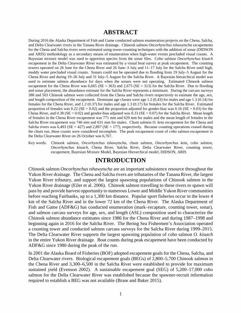
LIST OF FIGURES Figure Page 1. Map of the Chena River demarcating the Moose Creek Dam (river km 72) and the first bridge on
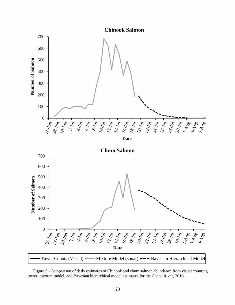
Chena Hot Springs Road (river km 161). ........................................................................................................ 4 2. Map of the Salcha River demarcating the counting tower............................................................................... 5 3. Map of the Delta Clearwater River demarcating the survey area .................................................................... 8 4. Estimates of Chinook salmon to the Chena and Salcha rivers with respective BEG ranges, 1986–2016. .... 22 5. Comparison of daily estimates of Chinook and chum salmon abundance from visual counting tower,
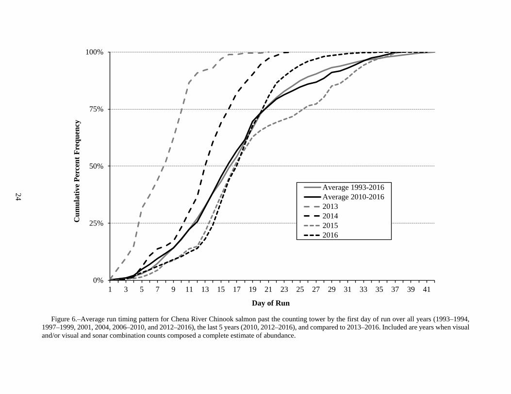
mixture model, and Bayesian hierarchical model estimates for the Chena River, 2016. .............................. 23 6. Average run timing pattern for Chena River Chinook salmon past the counting tower by the first day of
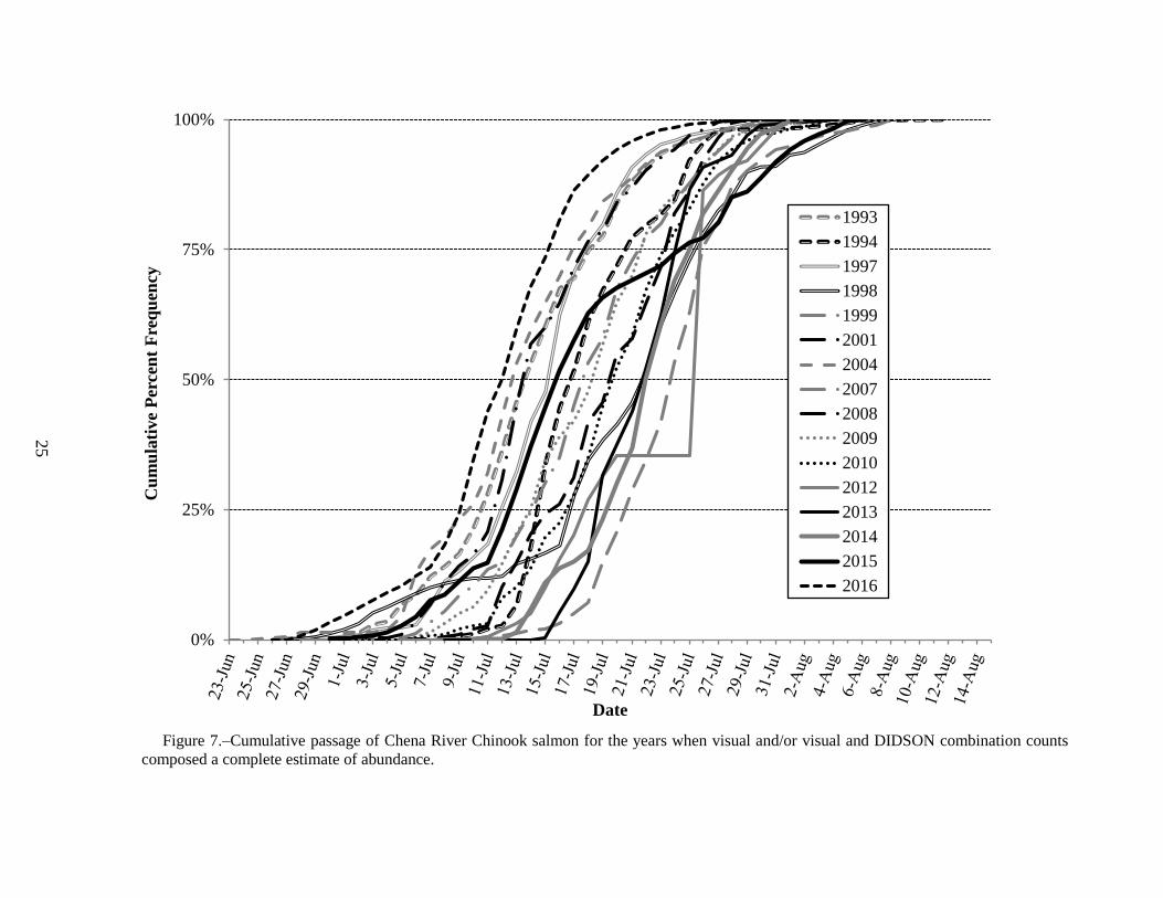
run over all years, the last 5 years, and compared to 2013–2016 .................................................................. 24 7. Cumulative passage of Chena River Chinook salmon for the years when visual and/or visual and
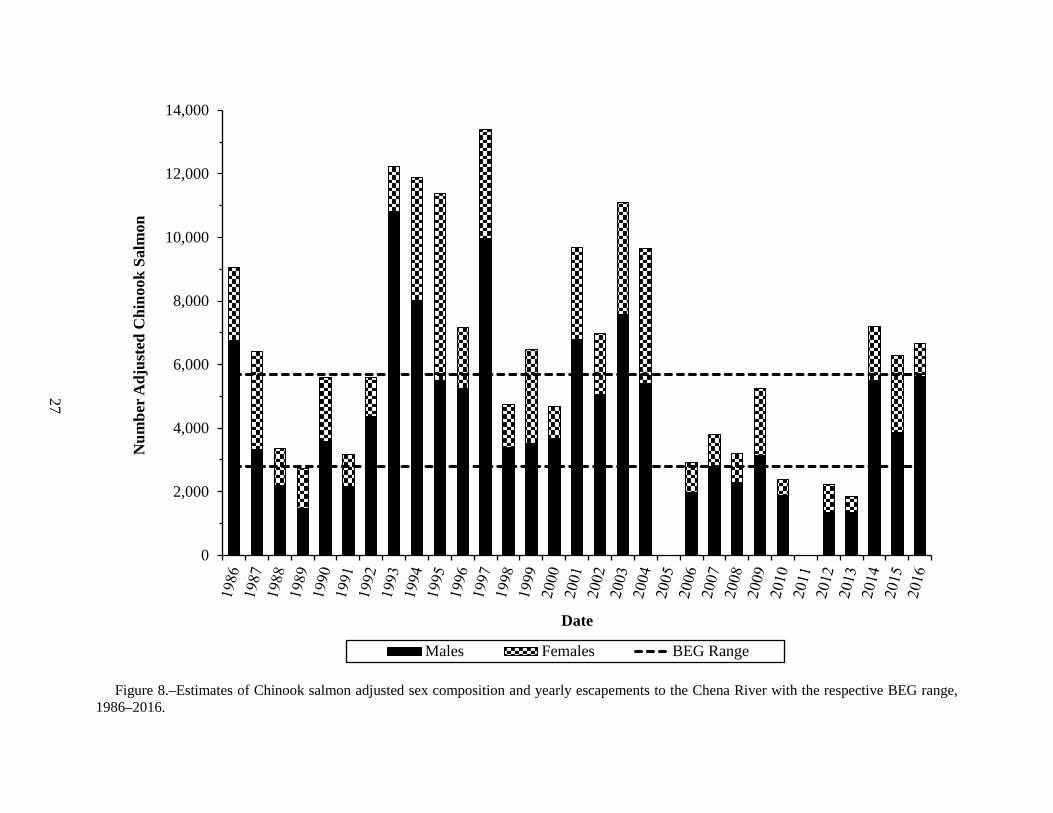
DIDSON combination counts composed a complete estimate of abundance. ............................................... 25 8. Estimates of Chinook salmon adjusted sex composition and yearly escapements to the Chena River
with the respective BEG range, 1986–2016. ................................................................................................. 27 9. Age proportions by year for Chinook salmon sampled from the Chena River during mark–recapture
events or carcass sampling ............................................................................................................................ 33 10. Comparison of daily estimates of Chinook and chum salmon abundance from visual counting tower,
mixture model, and Bayesian hierarchical model estimates for the Salcha River, 2016. .............................. 36 11. Average run timing pattern for Salcha River Chinook salmon past the counting tower by the first day
of run over all years, the last 5 years, and compared to 2013-2016 .............................................................. 37 12. Cumulative passage of Salcha River Chinook salmon for the years when visual and/or visual and sonar
combination counts composed a complete estimate of abundance. ............................................................... 38 13. Estimates of Chinook salmon adjusted sex composition and yearly escapements to the Salcha River
with the respective BEG range, 1986–2016. ................................................................................................. 40 14. Age proportions by year for Chinook salmon sampled from the Salcha River during mark–recapture
events or carcass sampling ............................................................................................................................ 46
LIST OF APPENDICES Appendix Page A1. JAGS code of mixture model. ....................................................................................................................... 56 B1. JAGS code of Bayesian Hierarchical Model ................................................................................................. 62
1
ABSTRACT During 2016 the Alaska Department of Fish and Game conducted salmon enumeration projects on the Chena, Salcha, and Delta Clearwater rivers in the Tanana River drainage. Chinook salmon Oncorhynchus tshawytscha escapements for the Chena and Salcha rivers were estimated using tower-counting techniques with the addition of sonar (DIDSON and ARIS) methodology as a secondary means of enumeration when high-water events precluded visual counts. A Bayesian mixture model was used to apportion species from the sonar files. Coho salmon Oncorhynchus kisutch escapement in the Delta Clearwater River was estimated by a visual boat survey at peak escapement. The counting towers operated on 26 June for the Chena River and 26 June–3 July and 11–17 July for the Salcha River until high, muddy water precluded visual counts. Sonars could not be operated due to flooding from 19 July–5 August for the Chena River and during 19–26 July and 31 July–5 August for the Salcha River. A Bayesian hierarchical model was used to estimate salmon abundance for days when the sonars were not operating. Estimated Chinook salmon escapement for the Chena River was 6,665 (SE = 363) and 2,675 (SE = 313) for the Salcha River. Due to flooding and sonar placement, the abundance estimate for the Salcha River represents a minimum. During the carcass surveys 388 and 503 Chinook salmon were collected from the Chena and Salcha rivers respectively to estimate the age, sex, and length composition of the escapement. Dominant age classes were age 1.2 (0.43) for males and age 1.3 (0.14) for females for the Chena River, and 1.2 (0.37) for males and age 1.3 (0.17) for females for the Salcha River. Estimated proportion of females was 0.22 (SE = 0.02) and the proportion adjusted for gender-bias was 0.16 (SE = 0.03) for the Chena River, and 0.38 (SE = 0.02) and gender-bias adjusted was 0.33 (SE = 0.07) for the Salcha River. Mean length of females in the Chena River escapement was 771 mm and 629 mm for males and the mean length of females in the Salcha River escapement was 746 mm and 631 mm for males. Chum salmon O. keta escapement for the Chena and Salcha rivers was 6,493 (SE = 427) and 2,897 (SE = 177), respectively. Because counting operations ceased during the chum run, these counts were considered incomplete. The peak escapement count of coho salmon escapement in the Delta Clearwater River on 26 October was 6,767.
Key words: Chinook salmon, Oncorhynchus tshawytscha, chum salmon, Oncorhynchus keta, coho salmon, Oncorhynchus kisutch, Chena River, Salcha River, Delta Clearwater River, counting tower, escapement, Bayesian Mixture Model, Bayesian Hierarchical model, DIDSON, ARIS
INTRODUCTION Chinook salmon Oncorhynchus tshawytscha are an important subsistence resource throughout the Yukon River drainage. The Chena and Salcha rivers are tributaries of the Tanana River, the largest Yukon River tributary, and support the largest spawning populations of Chinook salmon in the Yukon River drainage (Eiler et al. 2006). Chinook salmon travelling to these rivers to spawn will pass by and provide harvest opportunity to numerous Lower and Middle Yukon River communities before reaching Fairbanks, up to a 1,300 km distance. Popular sport fisheries occur in the lower 4 km of the Salcha River and in the lower 72 km of the Chena River. The Alaska Department of Fish and Game (ADF&G) has conducted enumeration (mark–recapture, counting tower, sonar), and salmon carcass surveys for age, sex, and length (ASL) composition used to characterize the Chinook salmon abundance estimates since 1986 for the Chena River and during 1987–1998 and beginning again in 2016 for the Salcha River. The Bering Sea Fishermen’s Association operated a counting tower and conducted salmon carcass surveys for the Salcha River during 1999–2015. The Delta Clearwater River supports the largest spawning population of coho salmon O. kisutch in the entire Yukon River drainage. Boat counts during peak escapement have been conducted by ADF&G since 1980 during the peak of the run.
In 2001 the Alaska Board of Fisheries (BOF) adopted escapement goals for the Chena, Salcha, and Delta Clearwater rivers. Biological escapement goals (BEGs) of 2,800–5,700 Chinook salmon in the Chena River and 3,300–6,500 in the Salcha River were established to provide for maximum sustained yield (Evenson 2002). A sustainable escapement goal (SEG) of 5,200–17,000 coho salmon for the Delta Clearwater River was established because the spawner-recruit information required to establish a BEG was not available (Brase and Baker 2015).
2
Historically, Chinook salmon along with summer and fall chum salmon were targeted in the commercial fisheries. During the 10-year historical period of high production (1989–1998), commercial harvests of Chinook salmon in the Yukon River averaged approximately 100,000 fish (Estensen et al 2017). Due to poor returns, direct commercial gillnet (drift and set) fisheries for Chinook salmon have not taken place since 2007. Incidental harvest of Chinook salmon during summer and fall chum directed fisheries has taken place up through 2011 with an average 5-year harvest of 27,497 during 2010–2014 (Estensen et al. 2017). However, the commercial sale of all Chinook salmon, even those that have been captured incidentally, has been prohibited since 2012.
Chinook salmon are an important subsistence species throughout the Yukon River drainage. The current amounts necessary for subsistence (ANS) of Chinook salmon in the Alaskan Yukon River drainage was designated by the BOF in January 2013 to be 45,500–66,704 Chinook salmon. Since 2008, Chinook salmon harvests have been below the ANS. Preliminary 2013–2015 harvest values average approximately 13,135, 2,826, and 7,807 respectively (Estensen et al 2017). Actions by the BOF during 2015 provided flexibility to allow retention of some Chinook salmon caught in salmon gear (fish wheels, gillnets) set for other species to help meet ANS. Incidental harvest was justified based on inseason Chinook salmon run assessment projects (Estensen et al. 2017), including the Chena and Salcha rivers enumeration projects. However, harvest of Chinook salmon in the Tanana River subsistence fisheries was 46% below the recent 5-year average and 63% below the recent 10-year average (Estensen et al. 2017)
The Chena River Chinook salmon sport fishery takes place in the Chena River downstream from all spawning areas. The 5-year (2009–2013) average sport catch of Chinook salmon in the Chena River was 296 fish and the corresponding average harvest was 57 fish (Jennings et al. 2011a, 2011b, 2015; Romberg et al. In prep). A recent 5-year (2009–2013) average sport catch of Chinook salmon in the Salcha River was 713 fish and the corresponding average harvest was 174 fish (Jennings et al. 2011a, 2011b, 2015, Romberg, et al. In press). The 5-year (2009–2013) average sport catch of coho salmon in the Delta Clearwater River was 3,070 fish, and the corresponding average harvest was 147 fish (Jennings et al. 2011a, 2011b, 2015; Romberg et al. In prep).
Coho salmon are also an important subsistence species in the Yukon River. During 2011–2015 the average annual coho salmon subsistence harvest was 16,632, the average commercial harvest was 90,337, the average personal-use harvest was 152, and the average sport harvest was 662 (JTC 2017).
Meaningful biological escapement goals are established with long, unbroken data strings of escapement and composition estimates. Escapement and composition monitoring projects for the Chena and Salcha rivers are among the longest continuous Chinook salmon escapement data sets in the Yukon River drainage. The monitoring programs provide information on run magnitude and timing, which allows managers to modify fishing regulations to achieve the established escapement goals. In addition, annual Chinook salmon escapement assessments are important when examining the spawner-recruit relationships used to determine the escapement goals. The current BEG is evaluated every 3 years during the BOF with all additional years of acquired data.
3
OBJECTIVES The objectives in 2016 were to:
1. estimate the total escapement of Chinook salmon in the Chena and Salcha rivers using tower-counting techniques such that the estimates were within 15% of the true values 95% of the time and the potential for bias was minimized;
2. estimate ASL compositions of the escapement of Chinook salmon in the Chena and Salcha rivers such that estimated proportions were within 6 percentage points of the true proportions 95% of the time;
3. count coho salmon in the Delta Clearwater River from a drifting river boat during peak spawning to estimate minimum escapement;
4. deploy and maintain sonars each in the Chena and Salcha rivers to enumerate passing salmon during periods of high-water when tower counts could not be completed; and
5. count chum salmon in the Chena and Salcha rivers throughout the duration of the Chinook salmon run.
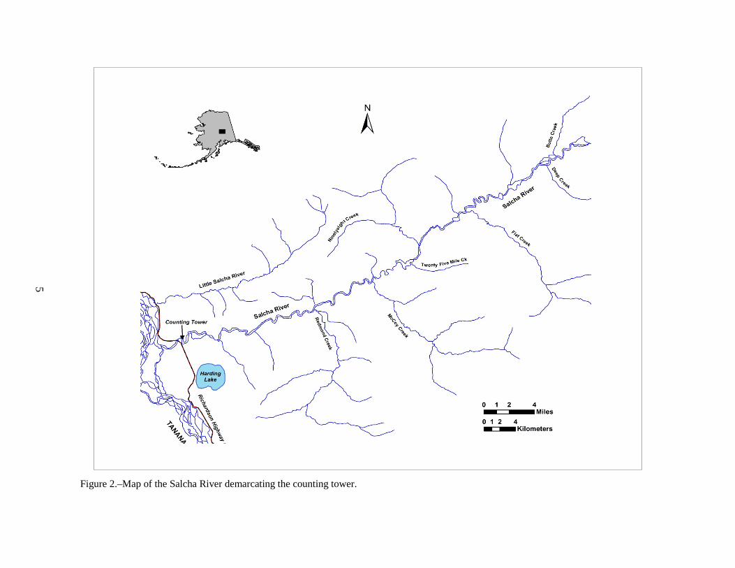
METHODS CHENA AND SALCHA RIVERS CHINOOK SALMON Daily escapements of Chinook and chum salmon were estimated by expansion of timed visual counts of fish as they passed over white fabric panels located on the river bottom on the upstream side of the Moose Creek Dam on the Chena River (Figure 1) and approximately 1 km upriver of the Richardson Highway Bridge (Figure 2) on the Salcha River. Personnel stood on top of scaffolding towers and counted all salmon passing upstream and downstream for 20-min intervals beginning at the top of every hour over the course of the run. Lights were suspended over the panels to provide illumination during periods of low ambient light. Counting was set to begin on or about 25 June and continue until there were 3 continuous days with no net upstream passage of Chinook salmon, typically around 5 August. The majority of Chinook salmon spawning occurred upstream of these sites; because no harvest of salmon is allowed on these river sections, final estimates represented total escapement.
The numbers of Chinook and chum salmon passing upstream and downstream across the panels were recorded on field forms at the end of each 20-min count. Only counts with an associated water clarity rating of 3 or lower were used in the estimate of escapement (Table 1). A count with an associated water clarity rating of 4 or 5 was considered as no count. Five technicians were assigned to each river to enumerate the salmon escapement. Each day was divided into three 8.0-hour shifts: Shift I began at 0000 (midnight) and ended at 0759, Shift II began at 0800 and ended at 1559, and Shift III began at 1600 and ended at 2359.
4
Figure 1.–Map of the Chena River demarcating the Moose Creek Dam (river km 72) and the first bridge on Chena Hot Springs Road (river
km 161).
5
Figure 2.–Map of the Salcha River demarcating the counting tower.

6
Table 1.–Water clarity ratings.
Rating Description Salmon Viewing Water Condition
1 Excellent All passing salmon are observable Virtually no turbidity or glare, “drinking water” clarity; all routes of passage observable
2 Good All passing salmon are observable Minimal to moderate levels of turbidity or glare; all routes of passage observable
3 Fair Possible, but not likely, that some passing salmon may be missed
Moderate to high levels of turbidity or glare; a few likely routes of passage are partially obscured
4 Poor Likely that some passing salmon may be missed
Moderate to high levels of turbidity or glare; some-many likely routes of passage are obscured
5 Un-observable Passing fish are not observable High level of turbidity or glare; ALL routes of passage obscured
In conjunction with the counting towers, two sonars were deployed upstream of the white fabric panels on the Salcha and Chena rivers to estimate the number of migrating salmon during periods of high-water. Two dual-frequency identification sonars (DIDSONs) were deployed on the Chena River on opposite sides of the counting tower, and one DIDSON and one adaptive resolution imaging sonar (ARIS) with a telephoto lens were deployed on the west side near the Salcha River counting tower. Ranges up to 30 m were needed to ensonify the entire river sections, and Burwen et al. (2007) established that standard DIDSON sonar units can precisely measure fish length up to 12 m away from the sonar unit on high frequency. The ARIS easily covered 15 meters on high frequency and the DIDSONs 10 m. Therefore, each sonar was positioned to cover half of the rivers such that the beams did not overlap and record a salmon twice. Images were recorded 24 hours a day, 7 days a week for the project duration. The DIDSONs were mounted to portable aluminum stands that could be moved manually to adjust for water depth. The ARIS also incorporated a rotator that enabled remote adjustment and focusing. Weir structures were deployed behind each unit to ensure migrating salmon passed through the sonar beam. When daily visual counts were available, the paired estimates were used to evaluate the effectiveness of the sonar in filling in for missing visual count days.
During and after the season, all fish >400 mm in length in the DIDSON sonar images were measured and recorded using Echotastic, a software program developed to process sonar images (Pfisterer 2010). Historical length distributions of chum and Chinook salmon from the Chena and Salcha rivers have illustrated that no salmon are less than 400 mm in length. The estimated lengths from the sonar images, along with the associated dates of tower passage, were later used in a Bayesian mixture model that also incorporated historical length and run-timing data to apportion and estimate numbers of Chinook and chum salmon from the total sonar count. Additionally, the Chinook salmon run was earlier, and they were usually larger than chum salmon. The mixture model used this information to apportion the total count by species.
Carcasses of spawned-out Chinook salmon were collected during the last week of July through the first 2 weeks of August from river km 72 to 161 (Figure 1) of the Chena River and from the
7
Richardson Highway Bridge (rkm 2) to Caribou Creek (88 rkm) on the Salcha River to estimate age, length, and sex composition of the escapement. Two riverboats with 3 people in each boat (1 operator and 2 people collecting carcasses) were used to collect Chinook salmon carcasses. Chinook salmon carcasses were speared from the boats and collected along banks and gravel bars. All deep pools and eddies that could be safely explored were inspected to find and sample as many Chinook salmon carcasses as possible. After collection, the carcasses were placed in a large tub onboard the boat. Once the tub was full, the boat landed on a gravel bar and the carcasses were laid out in rows with their left sides facing up. Measurements were made from mid-eye to fork of tail (METF). After sampling, the carcasses were cut in a distinctive manner through the left orbit to avoid resampling and returned to the river. Chum salmon were also collected and length and sex were also recorded. Information gathered was added to the mixture model that was used to apportion Chinook from chum salmon in the sonar data.
Ages were determined from scale patterns as described by Mosher (1969). Three scales were removed from the left side of the fish approximately 2 rows above the lateral line along a diagonal line downward from the posterior insertion of the dorsal fin to the anterior insertion of the anal fin (Welander 1940). If no scales were present in the preferred area due to decomposition, scales were removed from the same area on the right side of the fish or if necessary, from any location where there were any scales remaining, other than along the lateral line. Scales were stored in coin envelopes and later mounted on gum cards. Sex was determined from external and internal characteristics.
Objective criteria for ASL compositions were established to maintain the integrity of the spawner-recruit data used to calculate the BEGs. To estimate age compositions with the desired level of precision, a minimum of 416 Chinook salmon carcasses for each river were needed to achieve the objective for describing ASL estimates assuming 15% data loss due to unreadable scales (Thompson 1987).
Delta Clearwater River Coho Salmon Previous aerial surveys of the Delta Clearwater River drainage have shown that an average of 20% of the coho escapement is found in areas inaccessible to a boat survey (Parker 2009); therefore, counts of adult coho salmon were conducted to obtain a minimum estimate of escapement. This estimate was used to evaluate whether or not the SEG was met.
Two persons (a boat operator and a counter) conducted the survey from a drifting river boat equipped with a 5 ft elevated platform. The survey was done during peak spawning times over the course of 1 to 2 days along the lower 18 miles of the Delta Clearwater River to within 1.0 mile of the Clearwater Lake outlet (Figure 3). The total number of coho salmon observed (both dead and alive) were recorded every mile at mile markers posted on the river bank. The sum of the section counts equaled the estimate of minimum escapement.

8
Figure 3.–Map of the Delta Clearwater River demarcating the survey area (bold lines).
9
DATA ANALYSIS Chena and Salcha Rivers Chinook Salmon
Counting Towers Estimates of Chinook salmon escapement were stratified by day and daily estimates were summed to estimate total escapement. Daily escapement was estimated 1 of 5 ways, depending on the frequency of successful counts. The following criteria were used to determine the equations (1–15) used to estimate the daily escapement and its variance:
1. when 2 or more 8-hour shifts per day were considered complete (i.e., a minimum of 4 counting periods per shift were sampled), escapement for that day was estimated using equations 1–3 and variance was estimated using equations 4–8;
2. when only one 8-hour shift per day was considered complete but at least 4 counting periods are sampled, escapement for that day was estimated using equations 1–3 and variance was estimated using equation 13;
3. when no 8-hour shifts are considered complete on a given day, interpolation techniques described in equations 14 and 15 were used to estimate escapement, and equation 13 was used to estimate variance for inseason reporting of escapement estimates. This approach was used when no 8-hour shifts for 1 or 2 consecutive days of counting were considered complete. Postseason, escapement for these dates were estimated using the mixture model that apportions the sonar counts of salmon by species (Huang 2012, Stuby and Tyers 2016);
4. when all 8-hour shifts on 3 or more but fewer than 10 consecutive days were considered incomplete, no inseason daily escapement values were reported and postseason daily escapement values were assessed using a mixture model that apportions the sonar counts of salmon by species (Huang 2012, Stuby and Tyers 2016); and
5. when visual counting could not be conducted for an excessive number of days during the run (e.g., more than 10 consecutive days or more than 20 total days), or when neither visual counts or sonar counts could be conducted for 3 or more consecutive days (i.e., high water and inoperative sonar equipment), a Bayesian hierarchical model was used to estimate escapement for the missed days (if <25% total run) using characteristics of the run-timing curve (Hansen et al. 2016).
Although diel migratory patterns have been noted for other systems (Taras and Sarafin 2005), no distinct diel migratory pattern has been documented for Chena or Salcha River Chinook salmon (Stuby 2001; J. Savereide, ADF&G fishery biologist, Fairbanks, unpublished data).
Daily estimates of escapement were considered a two-stage direct expansion where the first stage is 8 h shifts within a day and the second stage was 20 min counting periods within a shift. The second stage was considered systematic sampling because the 20 min counting periods were not chosen randomly.
10
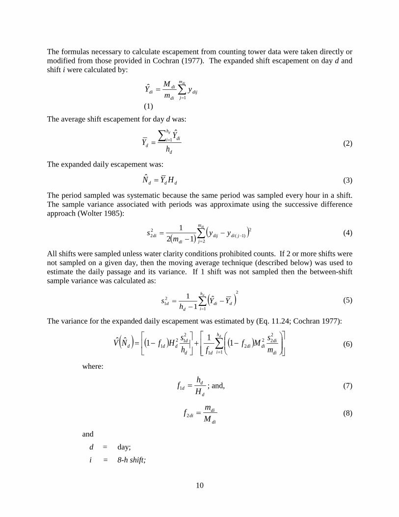
The formulas necessary to calculate escapement from counting tower data were taken directly or modified from those provided in Cochran (1977). The expanded shift escapement on day d and shift i were calculated by:
∑=
=dim
jdij
di
didi y
mM
Y1
ˆ
(1)
The average shift escapement for day d was:
d
h
i did h
YY
d∑== 1ˆ
(2)
The expanded daily escapement was:
ddd HYN =ˆ (3)
The period sampled was systematic because the same period was sampled every hour in a shift. The sample variance associated with periods was approximate using the successive difference approach (Wolter 1985):
( ) ( )∑=
−−−
=dim
jjdidij
didi yy
ms
2
2)1(
22 12
1 (4)
All shifts were sampled unless water clarity conditions prohibited counts. If 2 or more shifts were not sampled on a given day, then the moving average technique (described below) was used to estimate the daily passage and its variance. If 1 shift was not sampled then the between-shift sample variance was calculated as:
( )2
1
21
ˆ1
1 ∑=
−−
=dh
iddi
dd YY
hs (5)
The variance for the expanded daily escapement was estimated by (Eq. 11.24; Cochran 1977):
( ) ( ) ( )
−+
−= ∑
=
dh
i di
dididi
dd
dddd m
sMffh
sHfNV1
222
21
212
1 111ˆˆ (6)
where:
d
dd H
hf =1 ; and, (7)
di
didi M
mf =2 (8)
and
d = day;
i = 8-h shift;
11
j = 20-min counting period; ydij = observed 20-min period count;
𝑌𝑌�di = expanded shift escapement estimate; mdi = number of 20-min counting periods sampled within a shift;
Mdi = total number of possible 20-min counting periods within a day (24 would indicate a full day);
hd = number of 8-h shifts sampled within a day; Hd = total number of possible 8-h shifts within a day, D = total number of possible days.
f1 = fraction of 8-h shifts sampled; and,
f2 = fraction of 20 min counting periods sampled. Total escapement and variance estimates were the sum of all daily estimates:
∑=
=D
ddNN
1
ˆˆ ; and (9)
( ) ∑=
=D
ddNVNV
1)ˆ(ˆˆˆ (10)
Equation 5, the sample variance across shifts, requires data from more than 1 shift per day. In the event that water conditions and/or personnel constraints did not permit at least 2 shifts during a day, a coefficient of variation (CV) was calculated using all days when more than 1 shift was worked. The average CV was then used to approximate the daily variation for those days when fewer than 2 shifts were worked. The coefficient of variation was used because it is independent of the magnitude of the estimate and is relatively constant throughout the run (Evenson 1995). The daily CV was calculated as:
ddd NSECV ˆ= (11)
For all L days of the run where more than one shift was worked, an average CV was calculated as:
LCVCVL
ll∑
=
=1
(12)
and variance of the escapement for days where one or zero shifts was worked was estimated as:
( ) 2)ˆ(ˆvar dd NCVN = (13)
12
When k consecutive days were not sampled due to adverse viewing conditions, the moving average estimate for the missing day i was calculated as:
∑∑
+
−=
+
−== ki
kij
ki
kij ji
sampledwasjdayI
NsampledwasjdayIN
)(
ˆ)(ˆ (14)
where:
otherwise
trueisConditionConditionI
=01
)( (15)
was an indicator function. The moving average procedure would only be applied for data gaps that did not exceed 3 days for inseason daily estimate reporting (9 consecutive 8-hr shifts). Postseason, all data gaps were assessed using a mixture model (Huang 2012, Stuby & Tyers 2016) applied to the sonar data for final estimates.
Carcass Surveys Biased estimates of sex composition were noted during mark-recapture experiments when sex ratios of Chinook salmon collected with electroshocking gear (First Event) were compared with those collected during carcass surveys (Second Event). In the mark–recapture studies, the ratio of the abundance estimates of females to total abundance was used to estimate the percent of females in the population. Diagnostic testing associated with the analysis of the mark–recapture data dictated whether first-event or second-event samples or both were used to estimate sex and age compositions, and whether those estimates would be considered unbiased. A comparison of sex composition estimates from mark-recapture methods revealed that carcass surveys tended to overestimate the proportions of females in the population (and conversely tended to underestimate the proportion of males). Mark–recapture data were available for 9 years from the Chena River (1989–1992, 1995–1997, 2000, and 2002) and 7 years from the Salcha River (1987–1992, 1996). Given past and present use of counting tower and sonar techniques since 1993, correction factors were developed and applied to sex composition estimates (specifically the proportion of females) in years when only a carcass survey was conducted for ASL based on the average of ratios of unbiased estimates from past mark-recapture experiments.
The escapement estimate was apportioned by sex prior to apportioning by age categories within each sex. Age compositions were reported using the European notation that includes the number of freshwater and ocean years of residence. For example, age 1.2 symbolizes 1 year of freshwater residence and 2 years in the ocean (4 years total age). The estimated proportions of males and females from carcass surveys were calculated using (Cochran 1977):
c
scsc n
yp =ˆ (16)
with variance:
[ ] ( )1ˆ1ˆ
ˆˆ−−
=c
scscsc n
pppV (17)
where ysc is the number of salmon of sex s observed during carcass surveys and nc is the total number of salmon of either sex observed during carcass surveys for s = m or f.
13
The adjustment factor necessary to compensate for the gender bias is R pˆ = 0.708 with
)ˆ(ˆ RV p = 0.018 for the Chena River and R pˆ = 0.867 with )ˆ(ˆ RV p = 0.030 for the Salcha River
(Doxey 2004). The bias-corrected estimate and variance (Goodman 1960) of the proportion of females, p fe
~ , is:
Rpp pfcfe ˆˆ~ = with )ˆ(ˆ)ˆ(ˆ)ˆ(ˆˆ)ˆ(ˆˆ)~(ˆ 22 pVRVpVRRVppV fcpfcppfcfe −+= (18)
The bias-corrected estimates and variance of the proportion of males are:
pp feme~1~ −= and )~(ˆ)~(ˆ pVpV
feme=
Escapement of each sex was then estimated by:
NpN sesˆ~ˆ = (19)
The variance for sN̂ in this case is (Goodman 1960):
( ) ( ) ( ) ( ) ( )NVpVpNVNpVNV sesesesˆˆ~ˆ~ˆˆˆ~ˆˆˆ 22 −+= (20)
The proportion of fish at age k by sex s for samples collected solely for ASL were calculated as:
s
sksk n
yp =ˆ (21)
where =skp̂ the estimated proportion of Chinook salmon that are age k; ysk = the number of Chinook salmon sampled that are age k and sex s; and, ns = the total number of Chinook salmon sampled of sex s. The variance of this proportion was estimated as:
[ ] ( )1ˆ1ˆˆˆ
−−
=s
sksksk n
pppV (22)
Mean lengths and associated variances were calculated for each sex and associated age class using:
𝑙𝑙�̅�𝑗 = ∑ 𝑙𝑙𝑗𝑗𝑛𝑛𝑗𝑗−1
𝑛𝑛𝑠𝑠; and (23)
𝑉𝑉�𝑙𝑙�̅�𝑗� = ∑ �𝑙𝑙𝑗𝑗−𝑙𝑙𝚥𝚥��𝑛𝑛𝑗𝑗=1
𝑛𝑛(𝑛𝑛−1) (24)
Escapement at age k for each sex was then estimated by:
ssksk NpN ˆˆˆ = (25)
The variance for skN̂ in this case is (Goodman 1960):
( ) ( ) ( ) ( ) ( )ssksksssksk NVpVpNVNpVNV ˆˆˆˆˆˆˆˆˆˆˆˆ 22 −+= (26)
14
Sonar Mixture Model The proportions of Chinook and chum salmon in the total sonar counts were estimated using a mixture model with fish length being the discriminating information, weakly informed by run timing. The probability density function (pdf) of length of fish i (yi) was modeled using a weighted mixture model,
𝑓𝑓(𝑦𝑦𝑖𝑖) = 𝑝𝑝𝑐𝑐,𝑖𝑖𝑓𝑓𝑐𝑐(𝑦𝑦𝑖𝑖) + 𝑝𝑝𝑘𝑘,𝑖𝑖𝑓𝑓𝑘𝑘(𝑦𝑦𝑖𝑖), (27)
0 ≤ 𝑝𝑝𝑐𝑐,𝑖𝑖, 𝑝𝑝𝑘𝑘,𝑖𝑖 ≤ 1, and 𝑝𝑝𝑐𝑐,𝑖𝑖 + 𝑝𝑝𝑘𝑘,𝑖𝑖 = 1
where )(yfcis the length distribution of chum salmon and )(yfk
is the length distribution of Chinook salmon; weights 𝑝𝑝𝑐𝑐,𝑖𝑖 and 𝑝𝑝𝑘𝑘,𝑖𝑖 were the probabilities of fish i being a chum or Chinook salmon, respectively.
There is a moderate difference in length between male and female Chinook and chum salmon. The length distribution (pdf) of either species can be expressed with a two-component sex mixture model as shown below,
1 1 2 2( ) ( ) ( )c c c c cf y f y f yθ θ= +
1 1 2 2( ) ( ) ( )k k k k kf y f y f yθ θ= + (28)
where 𝜃𝜃𝑐𝑐1 and 𝜃𝜃𝑐𝑐2 are the proportions of male and female chum salmon, respectively; and 𝜃𝜃𝑘𝑘1 and 𝜃𝜃𝑘𝑘2 are the proportions of male and female Chinook salmon, respectively. The proportions of males and females add up to 1 for each species. Distributions 𝑓𝑓𝑐𝑐𝑐𝑐(𝑦𝑦) and 𝑓𝑓𝑘𝑘𝑐𝑐(𝑦𝑦) were assumed to be normal for both sexes,
2( ) ~ ( , )cs cs csf y N µ σ 2( ) ~ ( , )ks ks ksf y N µ σ (29)
Prior information about the length means (µ) and variances (σ2) in equation (29) were found in other fishery research publications. For this study, prior information for Chinook and chum salmon length distributions were taken from the Arctic-Yukon-Kuskokwim (AYK) Database Management System. In addition, prior information for chum salmon length distribution was provided by Clark (1993).
Actual individual fish length (y) was not measured directly from individual fish and therefore was considered an unobserved variable. Instead, fish length was measured from sonar images. A linear relationship was assumed between sonar length (yobs,i) and the actual fish length (yi) for fish i. The sonar fish length (yobs,i) was modeled as a normal variable whose mean was a linear function of actual fish length (yi) (Equation 30),
, 1 2obs i i iy yβ β ε= + + (30)
where yobs refers to observed sonar length, which are the fish length measurements obtained from the sonar images; yi refers to the actual fish length; and the intercept β1 and slope β2 are unknown parameters of the linear relationship between yobs,i and yi. Paired data used to inform the relationship between yobs,i and yi were obtained from a tethered-fish experiment (conducted by D. Burwen and S. Fleischman, ADF&G, personal communication). The relationship between actual length and observed length was not assumed to be the same for the two sonar technologies
15
employed (DIDSON, ARIS with a telephoto lens), so the slope and intercept parameters associated with each technology were allowed to differ.
The mixture model (equations 27–30) contains unknown parameters including species probability parameters 𝑝𝑝𝑐𝑐 and 𝑝𝑝𝑘𝑘, sex proportion parameters θs, intercept parameter β1, and slope parameter β2. In order to estimate these unknown parameters, the mixture model was fitted using Markov Chain Monte Carlo (MCMC) as implemented in the statistical software package JAGS (Plummer 2003), called through the statistical software R (R Core Team 2014) using R package R2jags (Su and Yajima 2015).
According to Bayes’s Theorem, the posterior distributions of the unknown parameters are proportional to the likelihood of the data multiplied by the prior distributions of the parameters. The likelihood of the data collected followed the mixture model density function (Equation 27). The prior distributions of the sex ratio parameters θs were assigned a Dirichlet (α,γ) distribution. It has been noted since this project’s inception that the Chinook salmon run starts earlier and will usually peak before or during the early portion of the chum salmon run and that the proportion of the total run comprised of Chinook salmon has followed an approximate logistic trend over the course of the run. Therefore, species proportions parameters pc,d and pk,d for run day xd were assigned diffuse Dirichlet priors (ηd,ζd) that were calculated by run date according to:
dd
d xbb 101log +=
−η
η
tt ηζ −= 1 (31)
Hyperparameters b0 and b1 were estimated using logistic regression to model the relationship between run-timing and species in historical data. Because some variability in this relationship exists between years, the values of b0 and b1 that were used in the model were estimated in a hierarchical logistic regression model, in which logistic regression parameters for the Chena and Salcha rivers were treated as multivariate normal. This allowed for parameters to vary between years (but modeled as from the same underlying distribution) and to vary between rivers (but modeled as correlated). Chinook and chum salmon lengths were assigned normal priors, using data from the AYK Database Management System, as well as Clark (1993). The historic data used for model priors suggests that male and female chum salmon lengths are similar. Female chum salmon mean length was 553.0 mm (SE = 1.1 mm) and male chum salmon mean length was 583.6 mm (SE = 1.3 mm). Chinook salmon lengths vary moderately between sexes; female Chinook salmon had a mean length of 851.4 mm (SE = 0.8 mm) and male Chinook salmon had a mean length of 703.9 mm (SE = 1.3 mm). The regression parameters β1 and β2 were assigned diffuse normal priors. The Bayesian MCMC was conducted using JAGS with 3 chains and 100,000 iterations in each chain. The first 50,000 iterations in each chain were considered as burn-in and discarded.
Species totals were calculated every iteration of the MCMC procedure, thus giving posterior distributions of the escapement for each species. Escapement estimates and respective standard errors were then obtained by calculating the median and standard deviation of the posterior draws of species totals.
JAGS code for model fitting can be found in Appendix A.
16
Bayesian Hierarchical model In the event visual counting could not be conducted for an excessive number of days during the run (e.g., more than 10 consecutive days or more than 20 total days), or when neither visual counts or sonar counts could be conducted for 3 or more consecutive days (i.e., high water and inoperative sonar equipment), a Bayesian hierarchical model was used to estimate escapement for the missed days using characteristics of the run-timing curve (Hansen et al. 2016). As a safeguard against reporting spurious results, an estimate will not be reported if the Bayesian hierarchical model represents more than 25% of the total estimated run (Hamachan Hamazaki, ADF&G Division of Commercial Fisheries biometrician, Anchorage; personal communication).
Estimated daily counts for day d within year k were assumed to be normally distributed around either a lognormal, extreme-value, or log-logistic trends by date.
𝑁𝑁�𝑘𝑘[𝑑𝑑]~𝑁𝑁(𝜃𝜃𝑘𝑘[𝑑𝑑],𝜎𝜎𝜃𝜃2) (32)
The run-timing trends of year k were determined by 3 parameters: ak describes the amplitude of the run peak, μk describes the location by date of the run peak, and bk describes the width of the run peak. The functional forms are given below for the lognormal, extreme-value, and log-logistic trends, respectively, for run day xk[d].
𝜃𝜃𝑘𝑘[𝑑𝑑] = 𝑎𝑎𝑘𝑘𝑒𝑒�−0.5�
𝑙𝑙𝑛𝑛�𝑥𝑥𝑘𝑘[𝑑𝑑]𝜇𝜇𝑘𝑘
�
𝑏𝑏𝑗𝑗�
2
�
(33)
𝜃𝜃𝑘𝑘[𝑑𝑑] = 𝑎𝑎𝑘𝑘𝑒𝑒�−𝑒𝑒
�−𝑥𝑥𝑘𝑘[𝑑𝑑]−𝜇𝜇𝑘𝑘
𝑏𝑏𝑘𝑘�−�
𝑥𝑥𝑘𝑘[𝑑𝑑]−𝜇𝜇𝑘𝑘𝑏𝑏𝑘𝑘
�+1�
(34)
𝜃𝜃𝑘𝑘[𝑑𝑑] = 𝑎𝑎𝑘𝑘 ��𝑏𝑏𝑘𝑘𝜇𝜇𝑘𝑘
��𝑥𝑥𝑘𝑘[𝑑𝑑]𝜇𝜇𝑘𝑘
��𝑏𝑏𝑘𝑘−1�
�1+�𝑥𝑥𝑘𝑘[𝑑𝑑]𝜇𝜇𝑘𝑘
�𝑏𝑏𝑘𝑘�2 � (35)
The lognormal form was used in 2016, because it gave the most biologically reasonable results. Amplitude parameters ak for each year were considered independent between years, and were each given flat, noninformative priors. However, μk and bk for each year were treated as normally distributed from common distributions, according to:
𝜇𝜇𝑘𝑘~𝑁𝑁(𝜇𝜇0,𝜎𝜎𝜇𝜇2) (36)
𝑏𝑏𝑘𝑘~𝑁𝑁(𝑏𝑏0,𝜎𝜎𝑏𝑏2) (37)
with noninformative priors placed on parameters μ0, σμ2, b0, and σb2. All available years’ data were
incorporated into the model in order to fine-tune parameter estimates.
Because Chinook salmon spawning in the Chena and Salcha rivers have been observed to follow very similar run-timing profiles each year, the mean timing parameters μk for each river were not treated as independent; rather, one was modeled under the assumption that the difference between the two was normally distributed. This constraint allowed the model to have greater predictive power, particularly if counts were available for one river while a data gap existed for the other.
JAGS code for a current version of this model is provided in Appendix B.
17
Delta Clearwater River Coho Salmon The minimum escapement of coho salmon was estimated by:
∑=
=s
iiCE
1min
(38) where Ci = count of coho salmon in each mile section and s = number of mile sections.
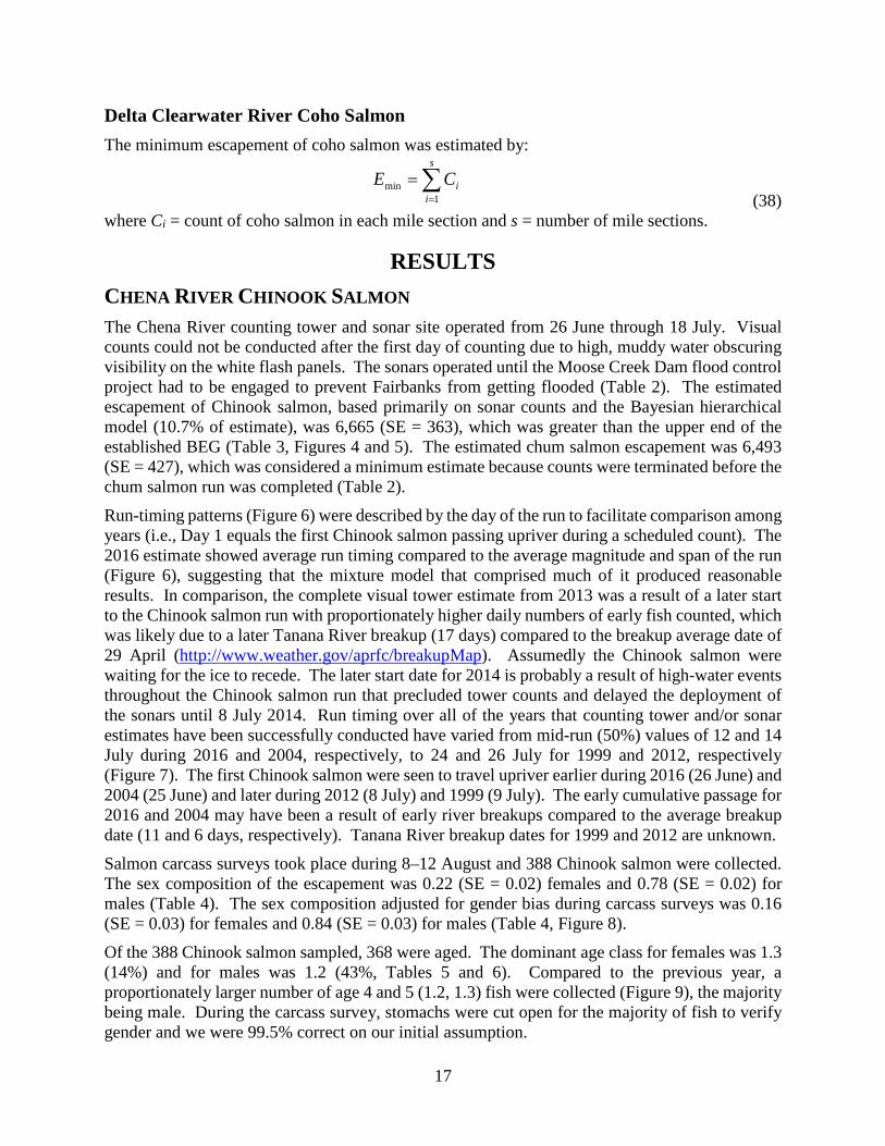
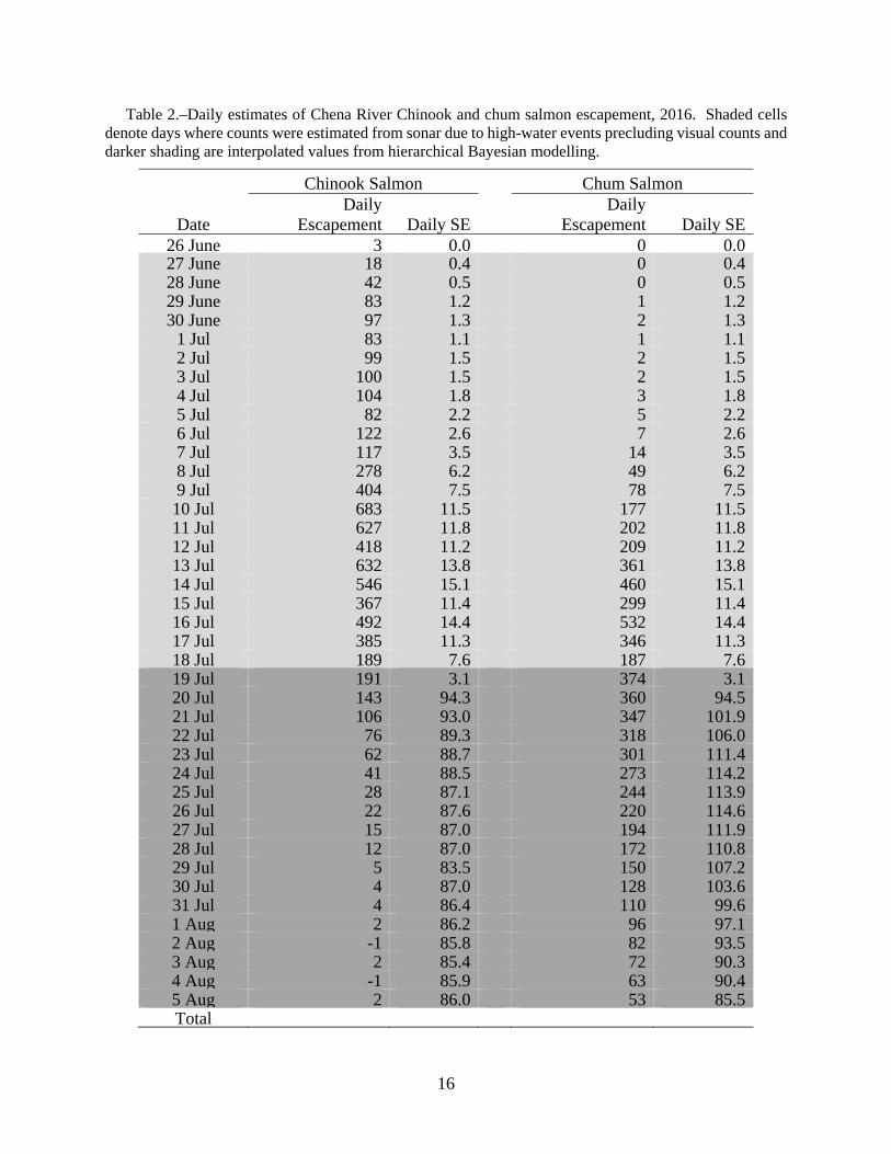
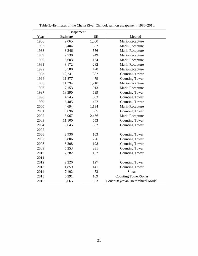
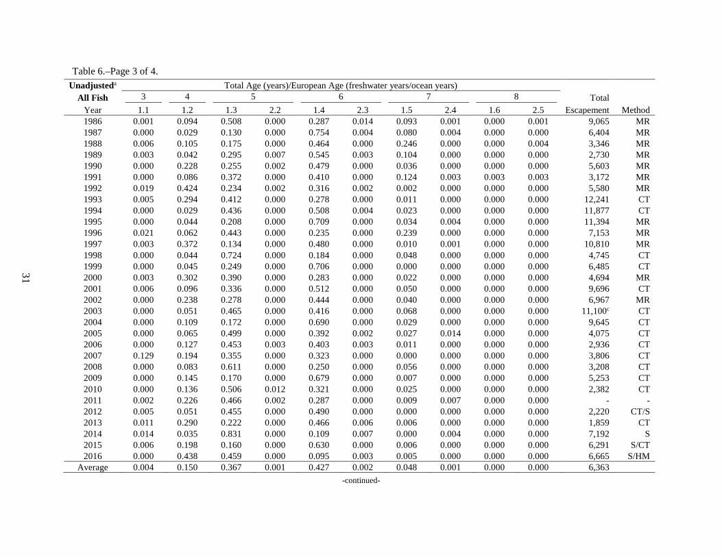
RESULTS CHENA RIVER CHINOOK SALMON The Chena River counting tower and sonar site operated from 26 June through 18 July. Visual counts could not be conducted after the first day of counting due to high, muddy water obscuring visibility on the white flash panels. The sonars operated until the Moose Creek Dam flood control project had to be engaged to prevent Fairbanks from getting flooded (Table 2). The estimated escapement of Chinook salmon, based primarily on sonar counts and the Bayesian hierarchical model (10.7% of estimate), was 6,665 (SE = 363), which was greater than the upper end of the established BEG (Table 3, Figures 4 and 5). The estimated chum salmon escapement was 6,493 (SE = 427), which was considered a minimum estimate because counts were terminated before the chum salmon run was completed (Table 2).
Run-timing patterns (Figure 6) were described by the day of the run to facilitate comparison among years (i.e., Day 1 equals the first Chinook salmon passing upriver during a scheduled count). The 2016 estimate showed average run timing compared to the average magnitude and span of the run (Figure 6), suggesting that the mixture model that comprised much of it produced reasonable results. In comparison, the complete visual tower estimate from 2013 was a result of a later start to the Chinook salmon run with proportionately higher daily numbers of early fish counted, which was likely due to a later Tanana River breakup (17 days) compared to the breakup average date of 29 April (http://www.weather.gov/aprfc/breakupMap). Assumedly the Chinook salmon were waiting for the ice to recede. The later start date for 2014 is probably a result of high-water events throughout the Chinook salmon run that precluded tower counts and delayed the deployment of the sonars until 8 July 2014. Run timing over all of the years that counting tower and/or sonar estimates have been successfully conducted have varied from mid-run (50%) values of 12 and 14 July during 2016 and 2004, respectively, to 24 and 26 July for 1999 and 2012, respectively (Figure 7). The first Chinook salmon were seen to travel upriver earlier during 2016 (26 June) and 2004 (25 June) and later during 2012 (8 July) and 1999 (9 July). The early cumulative passage for 2016 and 2004 may have been a result of early river breakups compared to the average breakup date (11 and 6 days, respectively). Tanana River breakup dates for 1999 and 2012 are unknown.
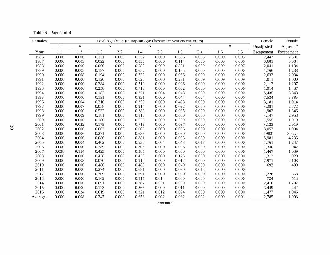
Salmon carcass surveys took place during 8–12 August and 388 Chinook salmon were collected. The sex composition of the escapement was 0.22 (SE = 0.02) females and 0.78 (SE = 0.02) for males (Table 4). The sex composition adjusted for gender bias during carcass surveys was 0.16 (SE = 0.03) for females and 0.84 (SE = 0.03) for males (Table 4, Figure 8).
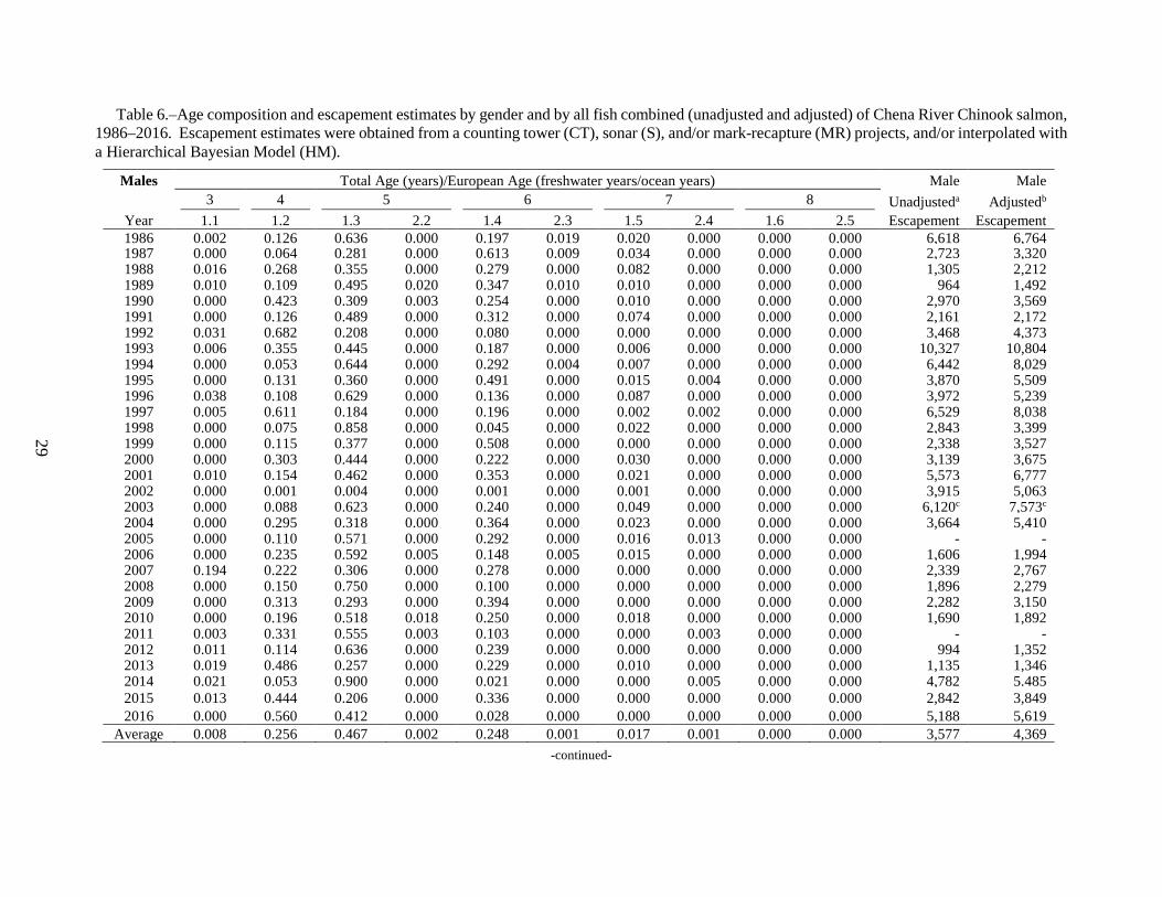
Of the 388 Chinook salmon sampled, 368 were aged. The dominant age class for females was 1.3 (14%) and for males was 1.2 (43%, Tables 5 and 6). Compared to the previous year, a proportionately larger number of age 4 and 5 (1.2, 1.3) fish were collected (Figure 9), the majority being male. During the carcass survey, stomachs were cut open for the majority of fish to verify gender and we were 99.5% correct on our initial assumption.
18
The average length for females was 771 mm (SE = 7) and for males was 629 mm (SE = 4, Table 5). Chum salmon were also sampled for sex and length data to add to the mixture model used to apportion Chinook from chum salmon in the sonar files. A total of 218 chum salmon were collected, of which 125 were males and 93 were females. Chum salmon lengths were an average of 577 mm for males and 536 mm for females.
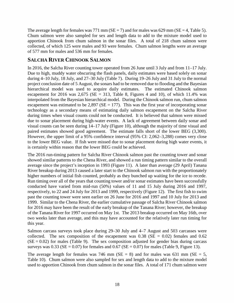
SALCHA RIVER CHINOOK SALMON In 2016, the Salcha River counting tower operated from 26 June until 3 July and from 11–17 July. Due to high, muddy water obscuring the flash panels, daily estimates were based solely on sonar during 4–10 July, 18 July, and 27–30 July (Table 7). During 19–26 July and 31 July to the normal project conclusion date of 5 August, the sonars had to be removed due to flooding and the Bayesian hierarchical model was used to acquire daily estimates. The estimated Chinook salmon escapement for 2016 was 2,675 (SE = 313, Table 8, Figures 4 and 10), of which 11.4% was interpolated from the Bayesian hierarchical model. During the Chinook salmon run, chum salmon escapement was estimated to be 2,897 (SE = 177). This was the first year of incorporating sonar technology as a secondary means of estimating daily salmon escapement on the Salcha River during times when visual counts could not be conducted. It is believed that salmon were missed due to sonar placement during high-water events. A lack of agreement between daily sonar and visual counts can be seen during 14–17 July (Figure 10), although the majority of time visual and paired estimates showed good agreement. The estimate falls short of the lower BEG (3,300). However, the upper limit of a 95% confidence interval (95% CI: 2,062–3,288) comes very close to the lower BEG value. If fish were missed due to sonar placement during high water events, it is certainly within reason that the lower BEG could be achieved.
The 2016 run-timing pattern for Salcha River Chinook salmon past the counting tower and sonar showed similar patterns to the Chena River, and showed a run timing pattern similar to the overall average since the project’s inception in 1993 (Figure 11). A later than average (29 April) Tanana River breakup during 2013 caused a later start to the Chinook salmon run with the proportionately higher numbers of initial fish counted, probably as they bunched up waiting for the ice to recede. Run timing over all of the years that counting tower and/or sonar estimates have been successfully conducted have varied from mid-run (50%) values of 11 and 15 July during 2016 and 1997, respectively, to 22 and 24 July for 2013 and 1999, respectively (Figure 12). The first fish to swim past the counting tower were seen earlier on 26 June for 2016 and 1997 and 10 July for 2013 and 1999. Similar to the Chena River, the earlier cumulative passage of Salcha River Chinook salmon for 2016 may have been the result of the early breakup of the Tanana River; however, the breakup of the Tanana River for 1997 occurred on May 1st. The 2013 breakup occurred on May 16th, over two weeks later than average, and this may have accounted for the relatively later run timing for this year.
Salmon carcass surveys took place during 29–30 July and 4–7 August and 503 carcasses were collected. The sex composition of the escapement was 0.38 (SE = 0.02) females and 0.62 (SE = 0.02) for males (Table 9). The sex composition adjusted for gender bias during carcass surveys was 0.33 (SE = 0.07) for females and 0.67 (SE = 0.07) for males (Table 9, Figure 13).
The average length for females was 746 mm (SE = 8) and for males was 631 mm (SE = 5, Table 10). Chum salmon were also sampled for sex and length data to add to the mixture model used to apportion Chinook from chum salmon in the sonar files. A total of 171 chum salmon were
19
collected, of which 82 were males and 89 were females. Average chum salmon lengths were an average of 582 mm for males and 553 mm for females.
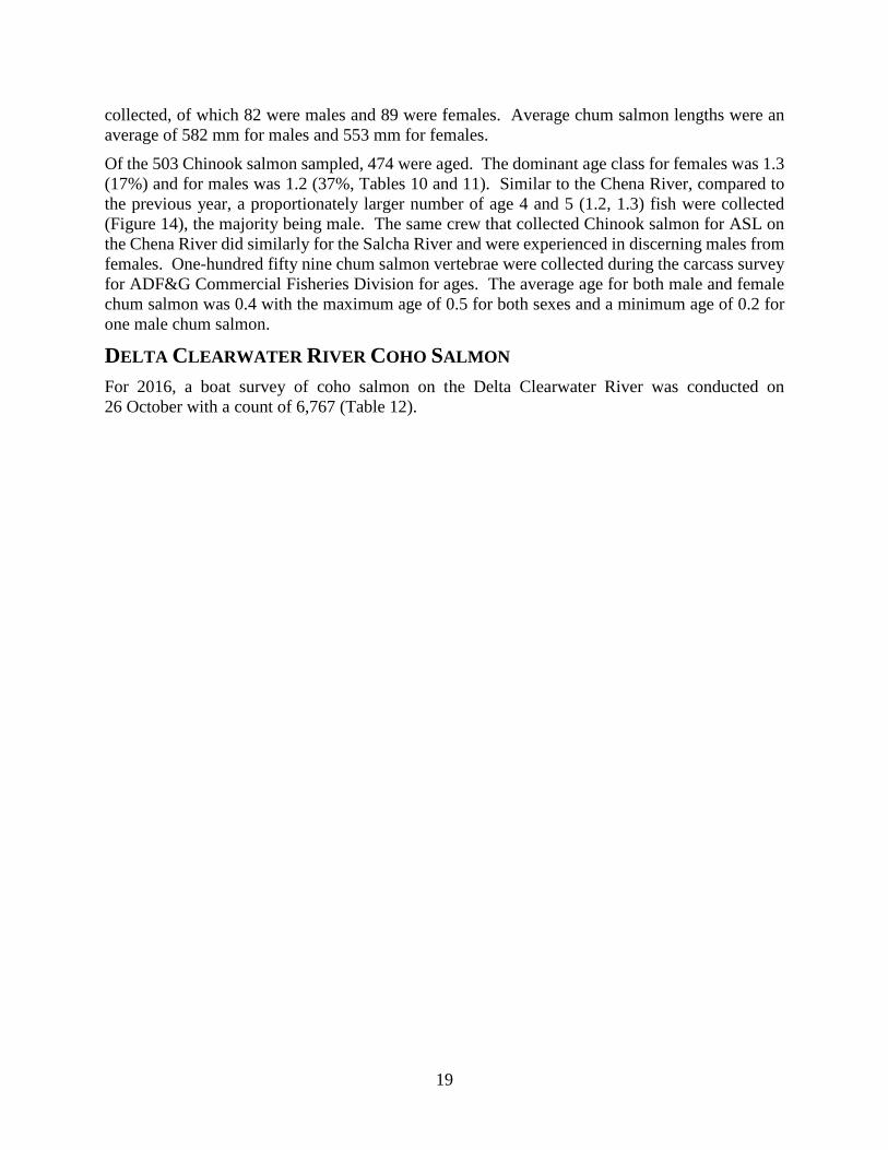
Of the 503 Chinook salmon sampled, 474 were aged. The dominant age class for females was 1.3 (17%) and for males was 1.2 (37%, Tables 10 and 11). Similar to the Chena River, compared to the previous year, a proportionately larger number of age 4 and 5 (1.2, 1.3) fish were collected (Figure 14), the majority being male. The same crew that collected Chinook salmon for ASL on the Chena River did similarly for the Salcha River and were experienced in discerning males from females. One-hundred fifty nine chum salmon vertebrae were collected during the carcass survey for ADF&G Commercial Fisheries Division for ages. The average age for both male and female chum salmon was 0.4 with the maximum age of 0.5 for both sexes and a minimum age of 0.2 for one male chum salmon.
DELTA CLEARWATER RIVER COHO SALMON For 2016, a boat survey of coho salmon on the Delta Clearwater River was conducted on 26 October with a count of 6,767 (Table 12).
16
Table 2.–Daily estimates of Chena River Chinook and chum salmon escapement, 2016. Shaded cells denote days where counts were estimated from sonar due to high-water events precluding visual counts and darker shading are interpolated values from hierarchical Bayesian modelling.
Chinook Salmon Chum Salmon
Date Daily
Escapement Daily SE Daily
Escapement Daily SE 26 June 3 0.0 0 0.0 27 June 18 0.4 0 0.4 28 June 42 0.5 0 0.5 29 June 83 1.2 1 1.2 30 June 97 1.3 2 1.3
1 Jul 83 1.1 1 1.1 2 Jul 99 1.5 2 1.5 3 Jul 100 1.5 2 1.5 4 Jul 104 1.8 3 1.8 5 Jul 82 2.2 5 2.2 6 Jul 122 2.6 7 2.6 7 Jul 117 3.5 14 3.5 8 Jul 278 6.2 49 6.2 9 Jul 404 7.5 78 7.5 10 Jul 683 11.5 177 11.5 11 Jul 627 11.8 202 11.8 12 Jul 418 11.2 209 11.2 13 Jul 632 13.8 361 13.8 14 Jul 546 15.1 460 15.1 15 Jul 367 11.4 299 11.4 16 Jul 492 14.4 532 14.4 17 Jul 385 11.3 346 11.3 18 Jul 189 7.6 187 7.6 19 Jul 191 3.1 374 3.1 20 Jul 143 94.3 360 94.5 21 Jul 106 93.0 347 101.9 22 Jul 76 89.3 318 106.0 23 Jul 62 88.7 301 111.4 24 Jul 41 88.5 273 114.2 25 Jul 28 87.1 244 113.9 26 Jul 22 87.6 220 114.6 27 Jul 15 87.0 194 111.9 28 Jul 12 87.0 172 110.8 29 Jul 5 83.5 150 107.2 30 Jul 4 87.0 128 103.6 31 Jul 4 86.4 110 99.6 1 Aug 2 86.2 96 97.1 2 Aug -1 85.8 82 93.5 3 Aug 2 85.4 72 90.3 4 Aug -1 85.9 63 90.4 5 Aug 2 86.0 53 85.5 Total
21
Table 3.–Estimates of the Chena River Chinook salmon escapement, 1986–2016.
Escapement Year Estimate SE Method
1986 9,065 1,080 Mark–Recapture 1987 6,404 557 Mark–Recapture 1988 3,346 556 Mark–Recapture 1989 2,730 249 Mark–Recapture 1990 5,603 1,164 Mark–Recapture 1991 3,172 282 Mark–Recapture 1992 5,580 478 Mark–Recapture 1993 12,241 387 Counting Tower 1994 11,877 479 Counting Tower 1995 11,394 1,210 Mark–Recapture 1996 7,153 913 Mark–Recapture 1997 13,390 699 Counting Tower 1998 4,745 503 Counting Tower 1999 6,485 427 Counting Tower 2000 4,694 1,184 Mark–Recapture 2001 9,696 565 Counting Tower 2002 6,967 2,466 Mark–Recapture 2003 11,100 653 Counting Tower 2004 9,645 532 Counting Tower 2005 - - - 2006 2,936 163 Counting Tower 2007 3,806 226 Counting Tower 2008 3,208 198 Counting Tower 2009 5,253 231 Counting Tower 2010 2,382 152 Counting Tower 2011 - - - 2012 2,220 127 Counting Tower 2013 1,859 141 Counting Tower 2014 7,192 73 Sonar 2015 6,291 169 Counting Tower/Sonar 2016 6,665 363 Sonar/Bayesian Hierarchical Model

22
Figure 4.–Estimates of Chinook salmon to the Chena and Salcha rivers with respective BEG ranges, 1986–2016.
0
2,000
4,000
6,000
8,000
10,000
12,000
14,000
16,000
18,000
20,000
Year
Chena RiverSalcha RiverChena River BEG RangeSalcha River BEG Range
Num
ber
of C
hino
ok sa
lmon
23
Figure 5.–Comparison of daily estimates of Chinook and chum salmon abundance from visual counting
tower, mixture model, and Bayesian hierarchical model estimates for the Chena River, 2016.
0
100
200
300
400
500
600
700N
umbe
r of
Sal
mon
Date
Chinook Salmon
0
100
200
300
400
500
600
700
Num
ber
of S
alm
on
Date
Chum Salmon
Tower Counts (Visual) Mixture Model (sonar) Bayesian Hierarchical Model
24
Figure 6.–Average run timing pattern for Chena River Chinook salmon past the counting tower by the first day of run over all years (1993–1994,
1997–1999, 2001, 2004, 2006–2010, and 2012–2016), the last 5 years (2010, 2012–2016), and compared to 2013–2016. Included are years when visual and/or visual and sonar combination counts composed a complete estimate of abundance.
0%
25%
50%
75%
100%
1 3 5 7 9 11 13 15 17 19 21 23 25 27 29 31 33 35 37 39 41
Cum
ulat
ive
Perc
ent F
requ
ency
Day of Run
Average 1993-2016Average 2010-20162013201420152016
25
Figure 7.–Cumulative passage of Chena River Chinook salmon for the years when visual and/or visual and DIDSON combination counts
composed a complete estimate of abundance.
0%
25%
50%
75%
100%
Cum
ulat
ive
Perc
ent F
requ
ency
Date
1993199419971998199920012004200720082009201020122013201420152016
26
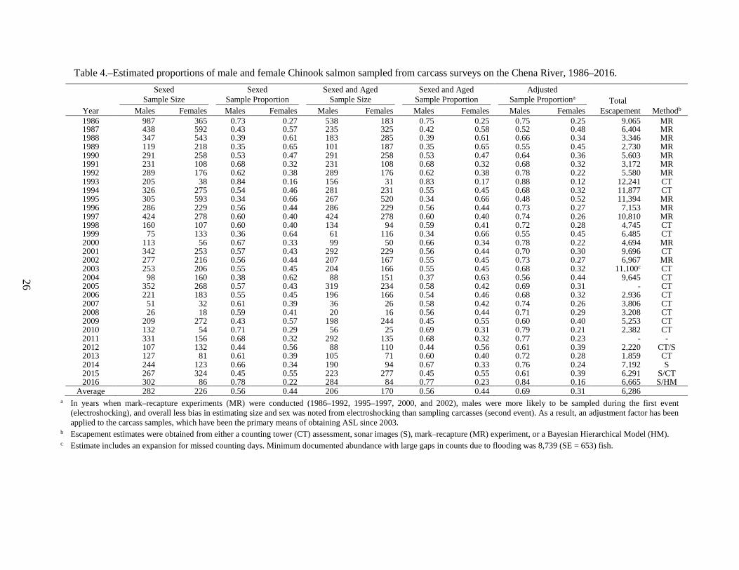
Table 4.–Estimated proportions of male and female Chinook salmon sampled from carcass surveys on the Chena River, 1986–2016.
Sexed Sexed Sexed and Aged Sexed and Aged Adjusted Sample Size Sample Proportion Sample Size Sample Proportion Sample Proportiona Total
Year Males Females Males Females Males Females Males Females Males Females Escapement Methodb
1986 987 365 0.73 0.27 538 183 0.75 0.25 0.75 0.25 9,065 MR 1987 438 592 0.43 0.57 235 325 0.42 0.58 0.52 0.48 6,404 MR 1988 347 543 0.39 0.61 183 285 0.39 0.61 0.66 0.34 3,346 MR 1989 119 218 0.35 0.65 101 187 0.35 0.65 0.55 0.45 2,730 MR 1990 291 258 0.53 0.47 291 258 0.53 0.47 0.64 0.36 5,603 MR 1991 231 108 0.68 0.32 231 108 0.68 0.32 0.68 0.32 3,172 MR 1992 289 176 0.62 0.38 289 176 0.62 0.38 0.78 0.22 5,580 MR 1993 205 38 0.84 0.16 156 31 0.83 0.17 0.88 0.12 12,241 CT 1994 326 275 0.54 0.46 281 231 0.55 0.45 0.68 0.32 11,877 CT 1995 305 593 0.34 0.66 267 520 0.34 0.66 0.48 0.52 11,394 MR 1996 286 229 0.56 0.44 286 229 0.56 0.44 0.73 0.27 7,153 MR 1997 424 278 0.60 0.40 424 278 0.60 0.40 0.74 0.26 10,810 MR 1998 160 107 0.60 0.40 134 94 0.59 0.41 0.72 0.28 4,745 CT 1999 75 133 0.36 0.64 61 116 0.34 0.66 0.55 0.45 6,485 CT 2000 113 56 0.67 0.33 99 50 0.66 0.34 0.78 0.22 4,694 MR 2001 342 253 0.57 0.43 292 229 0.56 0.44 0.70 0.30 9,696 CT 2002 277 216 0.56 0.44 207 167 0.55 0.45 0.73 0.27 6,967 MR 2003 253 206 0.55 0.45 204 166 0.55 0.45 0.68 0.32 11,100c CT 2004 98 160 0.38 0.62 88 151 0.37 0.63 0.56 0.44 9,645 CT 2005 352 268 0.57 0.43 319 234 0.58 0.42 0.69 0.31 - CT 2006 221 183 0.55 0.45 196 166 0.54 0.46 0.68 0.32 2,936 CT 2007 51 32 0.61 0.39 36 26 0.58 0.42 0.74 0.26 3,806 CT 2008 26 18 0.59 0.41 20 16 0.56 0.44 0.71 0.29 3,208 CT 2009 209 272 0.43 0.57 198 244 0.45 0.55 0.60 0.40 5,253 CT 2010 132 54 0.71 0.29 56 25 0.69 0.31 0.79 0.21 2,382 CT 2011 331 156 0.68 0.32 292 135 0.68 0.32 0.77 0.23 - - 2012 107 132 0.44 0.56 88 110 0.44 0.56 0.61 0.39 2,220 CT/S 2013 127 81 0.61 0.39 105 71 0.60 0.40 0.72 0.28 1,859 CT 2014 244 123 0.66 0.34 190 94 0.67 0.33 0.76 0.24 7,192 S 2015 267 324 0.45 0.55 223 277 0.45 0.55 0.61 0.39 6,291 S/CT 2016 302 86 0.78 0.22 284 84 0.77 0.23 0.84 0.16 6,665 S/HM
Average 282 226 0.56 0.44 206 170 0.56 0.44 0.69 0.31 6,286 a In years when mark–recapture experiments (MR) were conducted (1986–1992, 1995–1997, 2000, and 2002), males were more likely to be sampled during the first event
(electroshocking), and overall less bias in estimating size and sex was noted from electroshocking than sampling carcasses (second event). As a result, an adjustment factor has been applied to the carcass samples, which have been the primary means of obtaining ASL since 2003.
b Escapement estimates were obtained from either a counting tower (CT) assessment, sonar images (S), mark–recapture (MR) experiment, or a Bayesian Hierarchical Model (HM). c Estimate includes an expansion for missed counting days. Minimum documented abundance with large gaps in counts due to flooding was 8,739 (SE = 653) fish.
27
Figure 8.–Estimates of Chinook salmon adjusted sex composition and yearly escapements to the Chena River with the respective BEG range,
1986–2016.
0
2,000
4,000
6,000
8,000
10,000
12,000
14,000
Num
ber A
djus
ted
Chi
nook
Sal
mon
Date
Males Females BEG Range
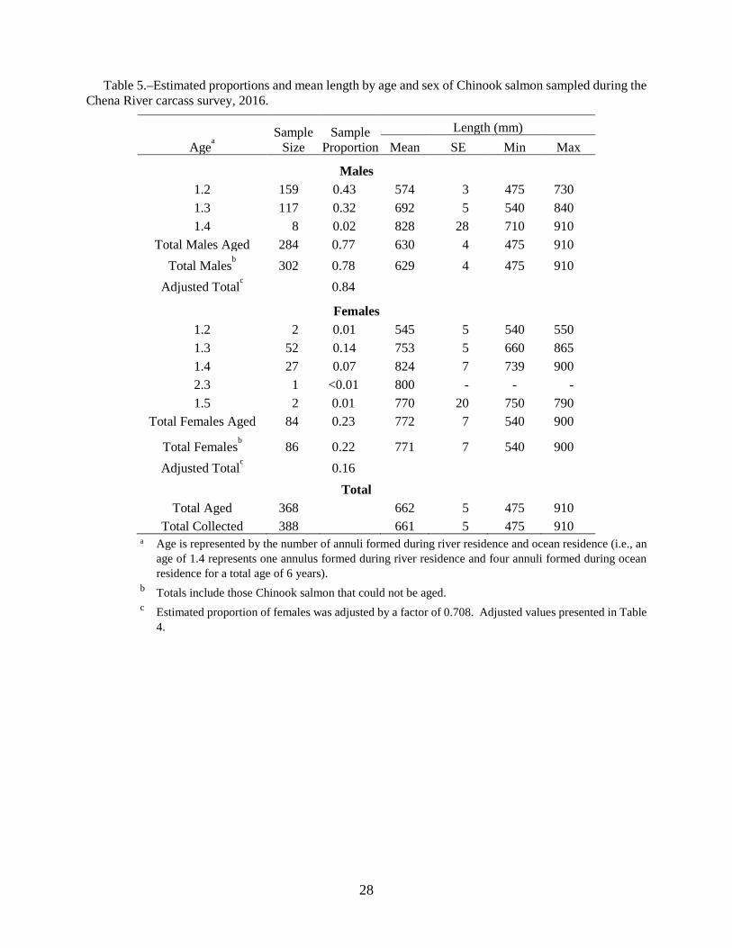
28
Table 5.–Estimated proportions and mean length by age and sex of Chinook salmon sampled during the Chena River carcass survey, 2016.
Sample Size
Sample Proportion
Length (mm) Agea Mean SE Min Max
Males 1.2 159 0.43 574 3 475 730 1.3 117 0.32 692 5 540 840 1.4 8 0.02 828 28 710 910
Total Males Aged 284 0.77 630 4 475 910 Total Malesb 302 0.78 629 4 475 910
Adjusted Totalc 0.84
Females 1.2 2 0.01 545 5 540 550 1.3 52 0.14 753 5 660 865 1.4 27 0.07 824 7 739 900 2.3 1 <0.01 800 - - - 1.5 2 0.01 770 20 750 790
Total Females Aged 84 0.23 772 7 540 900 Total Femalesb 86 0.22 771 7 540 900
Adjusted Totalc 0.16 Total
Total Aged 368 662 5 475 910 Total Collected 388 661 5 475 910
a Age is represented by the number of annuli formed during river residence and ocean residence (i.e., an age of 1.4 represents one annulus formed during river residence and four annuli formed during ocean residence for a total age of 6 years).
b Totals include those Chinook salmon that could not be aged. c Estimated proportion of females was adjusted by a factor of 0.708. Adjusted values presented in Table
4.
29
Table 6.–Age composition and escapement estimates by gender and by all fish combined (unadjusted and adjusted) of Chena River Chinook salmon, 1986–2016. Escapement estimates were obtained from a counting tower (CT), sonar (S), and/or mark-recapture (MR) projects, and/or interpolated with a Hierarchical Bayesian Model (HM).
Males Total Age (years)/European Age (freshwater years/ocean years) Male Male
3 4 5 6 7 8 Unadjusteda Adjustedb Year 1.1 1.2 1.3 2.2 1.4 2.3 1.5 2.4 1.6 2.5 Escapement Escapement 1986 0.002 0.126 0.636 0.000 0.197 0.019 0.020 0.000 0.000 0.000 6,618 6,764 1987 0.000 0.064 0.281 0.000 0.613 0.009 0.034 0.000 0.000 0.000 2,723 3,320 1988 0.016 0.268 0.355 0.000 0.279 0.000 0.082 0.000 0.000 0.000 1,305 2,212 1989 0.010 0.109 0.495 0.020 0.347 0.010 0.010 0.000 0.000 0.000 964 1,492 1990 0.000 0.423 0.309 0.003 0.254 0.000 0.010 0.000 0.000 0.000 2,970 3,569 1991 0.000 0.126 0.489 0.000 0.312 0.000 0.074 0.000 0.000 0.000 2,161 2,172 1992 0.031 0.682 0.208 0.000 0.080 0.000 0.000 0.000 0.000 0.000 3,468 4,373 1993 0.006 0.355 0.445 0.000 0.187 0.000 0.006 0.000 0.000 0.000 10,327 10,804 1994 0.000 0.053 0.644 0.000 0.292 0.004 0.007 0.000 0.000 0.000 6,442 8,029 1995 0.000 0.131 0.360 0.000 0.491 0.000 0.015 0.004 0.000 0.000 3,870 5,509 1996 0.038 0.108 0.629 0.000 0.136 0.000 0.087 0.000 0.000 0.000 3,972 5,239 1997 0.005 0.611 0.184 0.000 0.196 0.000 0.002 0.002 0.000 0.000 6,529 8,038 1998 0.000 0.075 0.858 0.000 0.045 0.000 0.022 0.000 0.000 0.000 2,843 3,399 1999 0.000 0.115 0.377 0.000 0.508 0.000 0.000 0.000 0.000 0.000 2,338 3,527 2000 0.000 0.303 0.444 0.000 0.222 0.000 0.030 0.000 0.000 0.000 3,139 3,675 2001 0.010 0.154 0.462 0.000 0.353 0.000 0.021 0.000 0.000 0.000 5,573 6,777 2002 0.000 0.001 0.004 0.000 0.001 0.000 0.001 0.000 0.000 0.000 3,915 5,063 2003 0.000 0.088 0.623 0.000 0.240 0.000 0.049 0.000 0.000 0.000 6,120c 7,573c 2004 0.000 0.295 0.318 0.000 0.364 0.000 0.023 0.000 0.000 0.000 3,664 5,410 2005 0.000 0.110 0.571 0.000 0.292 0.000 0.016 0.013 0.000 0.000 - - 2006 0.000 0.235 0.592 0.005 0.148 0.005 0.015 0.000 0.000 0.000 1,606 1,994 2007 0.194 0.222 0.306 0.000 0.278 0.000 0.000 0.000 0.000 0.000 2,339 2,767 2008 0.000 0.150 0.750 0.000 0.100 0.000 0.000 0.000 0.000 0.000 1,896 2,279 2009 0.000 0.313 0.293 0.000 0.394 0.000 0.000 0.000 0.000 0.000 2,282 3,150 2010 0.000 0.196 0.518 0.018 0.250 0.000 0.018 0.000 0.000 0.000 1,690 1,892 2011 0.003 0.331 0.555 0.003 0.103 0.000 0.000 0.003 0.000 0.000 - - 2012 0.011 0.114 0.636 0.000 0.239 0.000 0.000 0.000 0.000 0.000 994 1,352 2013 0.019 0.486 0.257 0.000 0.229 0.000 0.010 0.000 0.000 0.000 1,135 1,346 2014 0.021 0.053 0.900 0.000 0.021 0.000 0.000 0.005 0.000 0.000 4,782 5.485 2015 0.013 0.444 0.206 0.000 0.336 0.000 0.000 0.000 0.000 0.000 2,842 3,849 2016 0.000 0.560 0.412 0.000 0.028 0.000 0.000 0.000 0.000 0.000 5,188 5,619
Average 0.008 0.256 0.467 0.002 0.248 0.001 0.017 0.001 0.000 0.000 3,577 4,369 -continued-
30
Table 6.–Page 2 of 4.
Females Total Age (years)/European Age (freshwater years/ocean years) Female Female 3 4 5 6 7 8 Unadjusteda Adjustedb
Year 1.1 1.2 1.3 2.2 1.4 2.3 1.5 2.4 1.6 2.5 Escapement Escapement 1986 0.000 0.000 0.131 0.000 0.552 0.000 0.306 0.005 0.000 0.005 2,447 2,301 1987 0.000 0.003 0.022 0.000 0.855 0.000 0.114 0.006 0.000 0.000 3,681 3,084 1988 0.000 0.000 0.060 0.000 0.582 0.000 0.351 0.000 0.000 0.007 2,041 1,134 1989 0.000 0.005 0.187 0.000 0.652 0.000 0.155 0.000 0.000 0.000 1,766 1,238 1990 0.000 0.008 0.194 0.000 0.733 0.000 0.066 0.000 0.000 0.000 2,633 2,034 1991 0.000 0.000 0.120 0.000 0.620 0.000 0.231 0.009 0.009 0.009 1,011 1,000 1992 0.000 0.000 0.284 0.000 0.710 0.000 0.006 0.000 0.000 0.000 2,112 1,207 1993 0.000 0.000 0.258 0.000 0.710 0.000 0.032 0.000 0.000 0.000 1,914 1,437 1994 0.000 0.000 0.182 0.000 0.771 0.004 0.043 0.000 0.000 0.000 5,435 3,848 1995 0.000 0.000 0.131 0.000 0.821 0.000 0.044 0.004 0.000 0.000 7,524 5,885 1996 0.000 0.004 0.210 0.000 0.358 0.000 0.428 0.000 0.000 0.000 3,181 1,914 1997 0.000 0.007 0.058 0.000 0.914 0.000 0.022 0.000 0.000 0.000 4,281 2,772 1998 0.000 0.000 0.532 0.000 0.383 0.000 0.085 0.000 0.000 0.000 1,902 1,346 1999 0.000 0.009 0.181 0.000 0.810 0.000 0.000 0.000 0.000 0.000 4,147 2,958 2000 0.000 0.000 0.180 0.000 0.620 0.000 0.200 0.000 0.000 0.000 1,555 1,019 2001 0.000 0.022 0.175 0.000 0.716 0.000 0.087 0.000 0.000 0.000 4,123 2,919 2002 0.000 0.000 0.003 0.000 0.005 0.000 0.006 0.000 0.000 0.000 3,052 1,904 2003 0.000 0.006 0.271 0.000 0.633 0.000 0.090 0.000 0.000 0.000 4,980c 3,527c 2004 0.000 0.000 0.086 0.000 0.881 0.000 0.033 0.000 0.000 0.000 5,981 4,235 2005 0.000 0.004 0.402 0.000 0.530 0.004 0.043 0.017 0.000 0.000 1,761 1,247 2006 0.000 0.000 0.289 0.000 0.705 0.000 0.006 0.000 0.000 0.000 1,330 942 2007 0.038 0.154 0.423 0.000 0.385 0.000 0.000 0.000 0.000 0.000 1,467 1,039 2008 0.000 0.000 0.438 0.000 0.438 0.000 0.125 0.000 0.000 0.000 1,312 929 2009 0.000 0.008 0.070 0.000 0.910 0.000 0.012 0.000 0.000 0.000 2,971 2,103 2010 0.000 0.000 0.480 0.000 0.480 0.000 0.040 0.000 0.000 0.000 692 490 2011 0.000 0.000 0.274 0.000 0.681 0.000 0.030 0.015 0.000 0.000 - - 2012 0.000 0.000 0.309 0.000 0.691 0.000 0.000 0.000 0.000 0.000 1,226 868 2013 0.000 0.000 0.169 0.000 0.817 0.014 0.000 0.000 0.000 0.000 724 513 2014 0.000 0.000 0.691 0.000 0.287 0.021 0.000 0.000 0.000 0.000 2,410 1,707 2015 0.000 0.000 0.123 0.000 0.866 0.000 0.011 0.000 0.000 0.000 3,449 2,442 2016 0.000 0.024 0.619 0.000 0.321 0.012 0.024 0.000 0.000 0.000 1,477 1,046
Average 0.000 0.008 0.247 0.000 0.658 0.002 0.082 0.002 0.000 0.001 2,785 1,993 -continued-
31
Table 6.–Page 3 of 4. Unadjusteda Total Age (years)/European Age (freshwater years/ocean years)
All Fish 3 4 5 6 7 8 Total Year 1.1 1.2 1.3 2.2 1.4 2.3 1.5 2.4 1.6 2.5 Escapement Method
1986 0.001 0.094 0.508 0.000 0.287 0.014 0.093 0.001 0.000 0.001 9,065 MR 1987 0.000 0.029 0.130 0.000 0.754 0.004 0.080 0.004 0.000 0.000 6,404 MR 1988 0.006 0.105 0.175 0.000 0.464 0.000 0.246 0.000 0.000 0.004 3,346 MR 1989 0.003 0.042 0.295 0.007 0.545 0.003 0.104 0.000 0.000 0.000 2,730 MR 1990 0.000 0.228 0.255 0.002 0.479 0.000 0.036 0.000 0.000 0.000 5,603 MR 1991 0.000 0.086 0.372 0.000 0.410 0.000 0.124 0.003 0.003 0.003 3,172 MR 1992 0.019 0.424 0.234 0.002 0.316 0.002 0.002 0.000 0.000 0.000 5,580 MR 1993 0.005 0.294 0.412 0.000 0.278 0.000 0.011 0.000 0.000 0.000 12,241 CT 1994 0.000 0.029 0.436 0.000 0.508 0.004 0.023 0.000 0.000 0.000 11,877 CT 1995 0.000 0.044 0.208 0.000 0.709 0.000 0.034 0.004 0.000 0.000 11,394 MR 1996 0.021 0.062 0.443 0.000 0.235 0.000 0.239 0.000 0.000 0.000 7,153 MR 1997 0.003 0.372 0.134 0.000 0.480 0.000 0.010 0.001 0.000 0.000 10,810 MR 1998 0.000 0.044 0.724 0.000 0.184 0.000 0.048 0.000 0.000 0.000 4,745 CT 1999 0.000 0.045 0.249 0.000 0.706 0.000 0.000 0.000 0.000 0.000 6,485 CT 2000 0.003 0.302 0.390 0.000 0.283 0.000 0.022 0.000 0.000 0.000 4,694 MR 2001 0.006 0.096 0.336 0.000 0.512 0.000 0.050 0.000 0.000 0.000 9,696 CT 2002 0.000 0.238 0.278 0.000 0.444 0.000 0.040 0.000 0.000 0.000 6,967 MR 2003 0.000 0.051 0.465 0.000 0.416 0.000 0.068 0.000 0.000 0.000 11,100c CT 2004 0.000 0.109 0.172 0.000 0.690 0.000 0.029 0.000 0.000 0.000 9,645 CT 2005 0.000 0.065 0.499 0.000 0.392 0.002 0.027 0.014 0.000 0.000 4,075 CT 2006 0.000 0.127 0.453 0.003 0.403 0.003 0.011 0.000 0.000 0.000 2,936 CT 2007 0.129 0.194 0.355 0.000 0.323 0.000 0.000 0.000 0.000 0.000 3,806 CT 2008 0.000 0.083 0.611 0.000 0.250 0.000 0.056 0.000 0.000 0.000 3,208 CT 2009 0.000 0.145 0.170 0.000 0.679 0.000 0.007 0.000 0.000 0.000 5,253 CT 2010 0.000 0.136 0.506 0.012 0.321 0.000 0.025 0.000 0.000 0.000 2,382 CT 2011 0.002 0.226 0.466 0.002 0.287 0.000 0.009 0.007 0.000 0.000 - - 2012 0.005 0.051 0.455 0.000 0.490 0.000 0.000 0.000 0.000 0.000 2,220 CT/S 2013 0.011 0.290 0.222 0.000 0.466 0.006 0.006 0.000 0.000 0.000 1,859 CT 2014 0.014 0.035 0.831 0.000 0.109 0.007 0.000 0.004 0.000 0.000 7,192 S 2015 0.006 0.198 0.160 0.000 0.630 0.000 0.006 0.000 0.000 0.000 6,291 S/CT 2016 0.000 0.438 0.459 0.000 0.095 0.003 0.005 0.000 0.000 0.000 6,665 S/HM
Average 0.004 0.150 0.367 0.001 0.427 0.002 0.048 0.001 0.000 0.000 6,363 -continued-
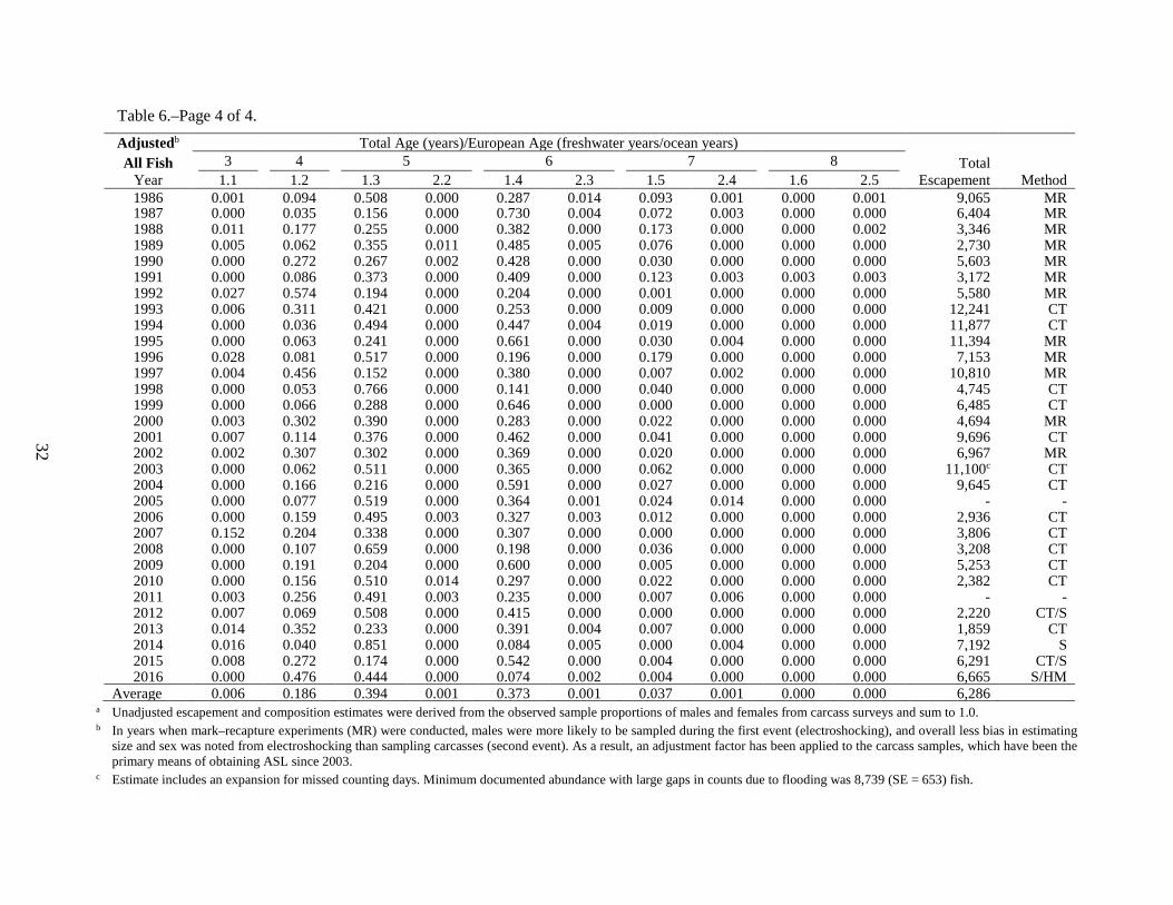
32
Table 6.–Page 4 of 4. Adjustedb Total Age (years)/European Age (freshwater years/ocean years) All Fish 3 4 5 6 7 8 Total
Year 1.1 1.2 1.3 2.2 1.4 2.3 1.5 2.4 1.6 2.5 Escapement Method
1986 0.001 0.094 0.508 0.000 0.287 0.014 0.093 0.001 0.000 0.001 9,065 MR 1987 0.000 0.035 0.156 0.000 0.730 0.004 0.072 0.003 0.000 0.000 6,404 MR 1988 0.011 0.177 0.255 0.000 0.382 0.000 0.173 0.000 0.000 0.002 3,346 MR 1989 0.005 0.062 0.355 0.011 0.485 0.005 0.076 0.000 0.000 0.000 2,730 MR 1990 0.000 0.272 0.267 0.002 0.428 0.000 0.030 0.000 0.000 0.000 5,603 MR 1991 0.000 0.086 0.373 0.000 0.409 0.000 0.123 0.003 0.003 0.003 3,172 MR 1992 0.027 0.574 0.194 0.000 0.204 0.000 0.001 0.000 0.000 0.000 5,580 MR 1993 0.006 0.311 0.421 0.000 0.253 0.000 0.009 0.000 0.000 0.000 12,241 CT 1994 0.000 0.036 0.494 0.000 0.447 0.004 0.019 0.000 0.000 0.000 11,877 CT 1995 0.000 0.063 0.241 0.000 0.661 0.000 0.030 0.004 0.000 0.000 11,394 MR 1996 0.028 0.081 0.517 0.000 0.196 0.000 0.179 0.000 0.000 0.000 7,153 MR 1997 0.004 0.456 0.152 0.000 0.380 0.000 0.007 0.002 0.000 0.000 10,810 MR 1998 0.000 0.053 0.766 0.000 0.141 0.000 0.040 0.000 0.000 0.000 4,745 CT 1999 0.000 0.066 0.288 0.000 0.646 0.000 0.000 0.000 0.000 0.000 6,485 CT 2000 0.003 0.302 0.390 0.000 0.283 0.000 0.022 0.000 0.000 0.000 4,694 MR 2001 0.007 0.114 0.376 0.000 0.462 0.000 0.041 0.000 0.000 0.000 9,696 CT 2002 0.002 0.307 0.302 0.000 0.369 0.000 0.020 0.000 0.000 0.000 6,967 MR 2003 0.000 0.062 0.511 0.000 0.365 0.000 0.062 0.000 0.000 0.000 11,100c CT 2004 0.000 0.166 0.216 0.000 0.591 0.000 0.027 0.000 0.000 0.000 9,645 CT 2005 0.000 0.077 0.519 0.000 0.364 0.001 0.024 0.014 0.000 0.000 - - 2006 0.000 0.159 0.495 0.003 0.327 0.003 0.012 0.000 0.000 0.000 2,936 CT 2007 0.152 0.204 0.338 0.000 0.307 0.000 0.000 0.000 0.000 0.000 3,806 CT 2008 0.000 0.107 0.659 0.000 0.198 0.000 0.036 0.000 0.000 0.000 3,208 CT 2009 0.000 0.191 0.204 0.000 0.600 0.000 0.005 0.000 0.000 0.000 5,253 CT 2010 0.000 0.156 0.510 0.014 0.297 0.000 0.022 0.000 0.000 0.000 2,382 CT 2011 0.003 0.256 0.491 0.003 0.235 0.000 0.007 0.006 0.000 0.000 - - 2012 0.007 0.069 0.508 0.000 0.415 0.000 0.000 0.000 0.000 0.000 2,220 CT/S 2013 0.014 0.352 0.233 0.000 0.391 0.004 0.007 0.000 0.000 0.000 1,859 CT 2014 0.016 0.040 0.851 0.000 0.084 0.005 0.000 0.004 0.000 0.000 7,192 S 2015 0.008 0.272 0.174 0.000 0.542 0.000 0.004 0.000 0.000 0.000 6,291 CT/S 2016 0.000 0.476 0.444 0.000 0.074 0.002 0.004 0.000 0.000 0.000 6,665
S/HM
Average 0.006 0.186 0.394 0.001 0.373 0.001 0.037 0.001 0.000 0.000 6,286
a Unadjusted escapement and composition estimates were derived from the observed sample proportions of males and females from carcass surveys and sum to 1.0. b In years when mark–recapture experiments (MR) were conducted, males were more likely to be sampled during the first event (electroshocking), and overall less bias in estimating
size and sex was noted from electroshocking than sampling carcasses (second event). As a result, an adjustment factor has been applied to the carcass samples, which have been the primary means of obtaining ASL since 2003.
c Estimate includes an expansion for missed counting days. Minimum documented abundance with large gaps in counts due to flooding was 8,739 (SE = 653) fish.
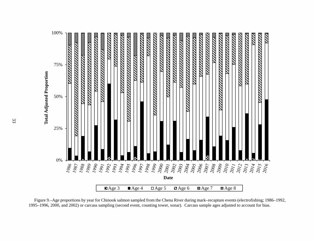
33
Figure 9.–Age proportions by year for Chinook salmon sampled from the Chena River during mark–recapture events (electrofishing; 1986–1992,
1995–1996, 2000, and 2002) or carcass sampling (second event, counting tower, sonar). Carcass sample ages adjusted to account for bias.
0%
25%
50%
75%
100%
Tota
l Adj
uste
d Pr
opor
tion
Date
Age 3 Age 4 Age 5 Age 6 Age 7 Age 8
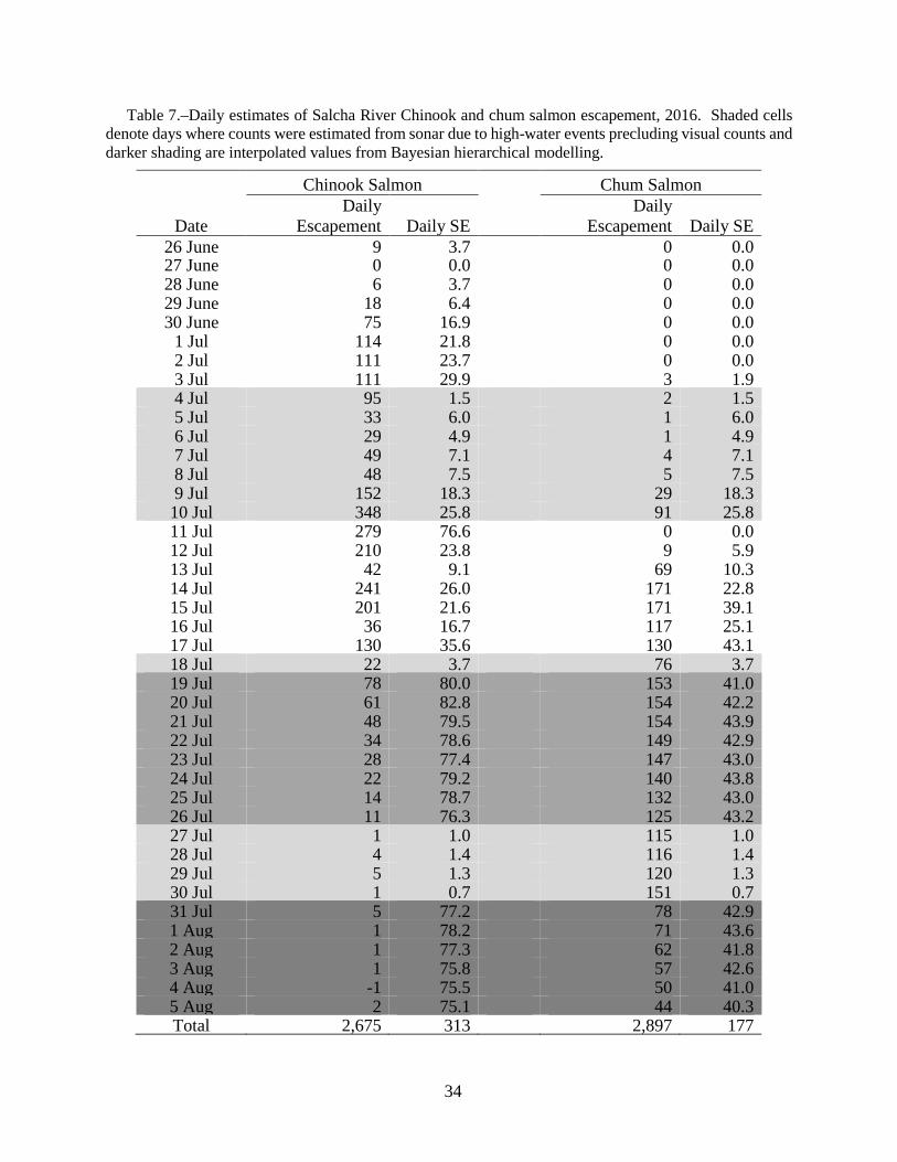
34
Table 7.–Daily estimates of Salcha River Chinook and chum salmon escapement, 2016. Shaded cells denote days where counts were estimated from sonar due to high-water events precluding visual counts and darker shading are interpolated values from Bayesian hierarchical modelling.
Chinook Salmon Chum Salmon
Date Daily
Escapement Daily SE Daily
Escapement Daily SE 26 June 9 3.7 0 0.0 27 June 0 0.0 0 0.0 28 June 6 3.7 0 0.0 29 June 18 6.4 0 0.0 30 June 75 16.9 0 0.0
1 Jul 114 21.8 0 0.0 2 Jul 111 23.7 0 0.0 3 Jul 111 29.9 3 1.9 4 Jul 95 1.5 2 1.5 5 Jul 33 6.0 1 6.0 6 Jul 29 4.9 1 4.9 7 Jul 49 7.1 4 7.1 8 Jul 48 7.5 5 7.5 9 Jul 152 18.3 29 18.3 10 Jul 348 25.8 91 25.8 11 Jul 279 76.6 0 0.0 12 Jul 210 23.8 9 5.9 13 Jul 42 9.1 69 10.3 14 Jul 241 26.0 171 22.8 15 Jul 201 21.6 171 39.1 16 Jul 36 16.7 117 25.1 17 Jul 130 35.6 130 43.1 18 Jul 22 3.7 76
3.7
19 Jul 78 80.0 153 41.0 20 Jul 61 82.8 154 42.2 21 Jul 48 79.5 154 43.9 22 Jul 34 78.6 149 42.9 23 Jul 28 77.4 147 43.0 24 Jul 22 79.2 140 43.8 25 Jul 14 78.7 132 43.0 26 Jul 11 76.3 125 43.2 27 Jul 1 1.0 115 1.0 28 Jul 4 1.4 116 1.4 29 Jul 5 1.3 120 1.3 30 Jul 1 0.7 151 0.7 31 Jul 5 77.2 78 42.9 1 Aug 1 78.2 71 43.6 2 Aug 1 77.3 62 41.8 3 Aug 1 75.8 57 42.6 4 Aug -1 75.5 50 41.0 5 Aug 2 75.1 44 40.3 Total 2,675 313 2,897 177
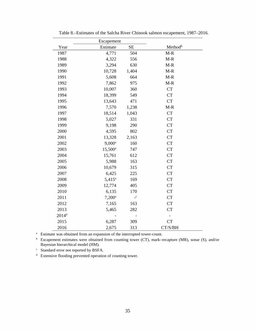
35
Table 8.–Estimates of the Salcha River Chinook salmon escapement, 1987–2016.
Escapement Year Estimate SE Methodb
1987 4,771 504 M-R 1988 4,322 556 M-R 1989 3,294 630 M-R 1990 10,728 1,404 M-R 1991 5,608 664 M-R 1992 7,862 975 M-R 1993 10,007 360 CT 1994 18,399 549 CT 1995 13,643 471 CT 1996 7,570 1,238 M-R 1997 18,514 1,043 CT 1998 5,027 331 CT 1999 9,198 290 CT 2000 4,595 802 CT 2001 13,328 2,163 CT 2002 9,000a 160 CT 2003 15,500a 747 CT 2004 15,761 612 CT 2005 5,988 163 CT 2006 10,679 315 CT 2007 6,425 225 CT 2008 5,415a 169 CT 2009 12,774 405 CT 2010 6,135 170 CT 2011 7,200a -c CT 2012 7,165 163 CT 2013 5,465 282 CT 2014d - - - 2015 6,287 309 CT 2016 2,675 313 CT/S/BH
a Estimate was obtained from an expansion of the interrupted tower-count. b Escapement estimates were obtained from counting tower (CT), mark–recapture (MR), sonar (S), and/or
Bayesian hierarchical model (HM). c Standard error not reported by BSFA. d Extensive flooding prevented operation of counting tower.
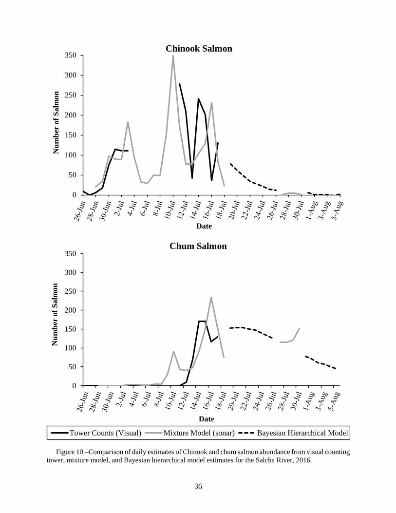
36
Figure 10.–Comparison of daily estimates of Chinook and chum salmon abundance from visual counting
tower, mixture model, and Bayesian hierarchical model estimates for the Salcha River, 2016.
0
50
100
150
200
250
300
350N
umbe
r of
Sal
mon
Date
Chinook Salmon
0
50
100
150
200
250
300
350
Num
ber
of S
alm
on
Date
Chum Salmon
Tower Counts (Visual) Mixture Model (sonar) Bayesian Hierarchical Model
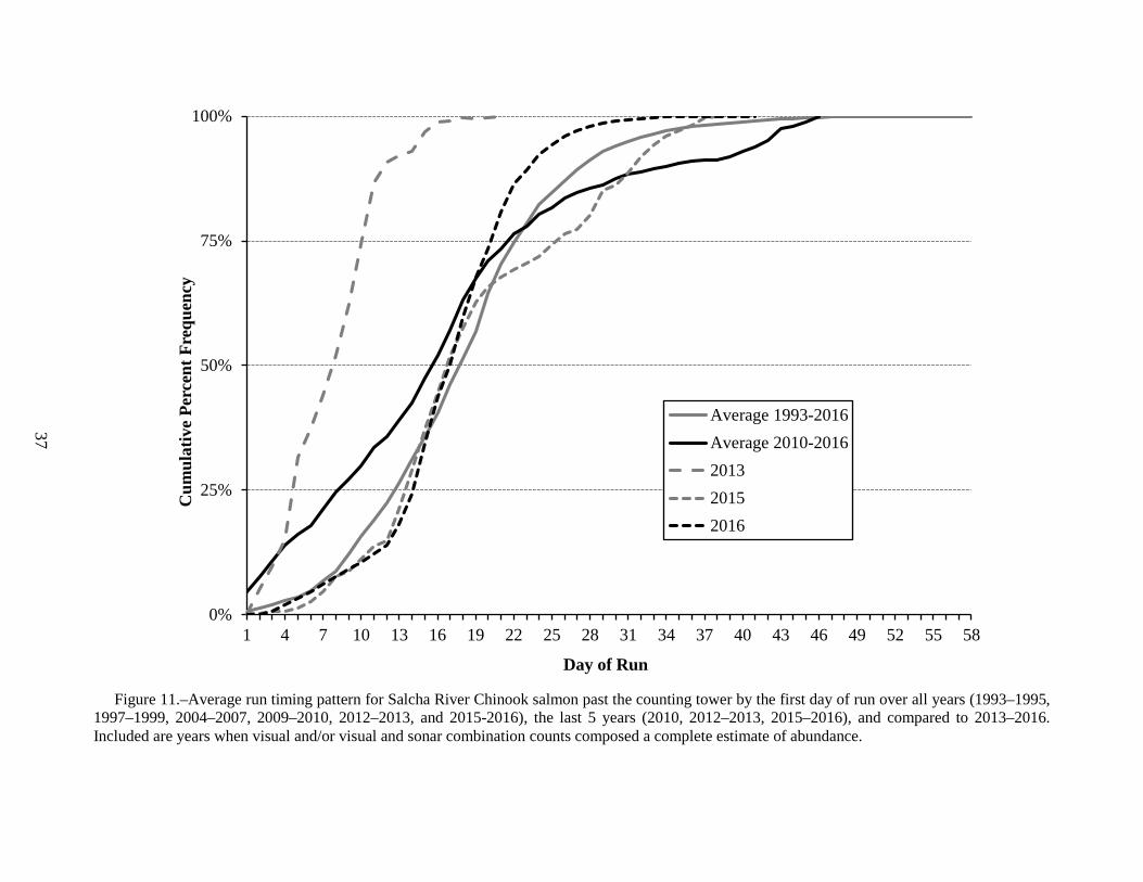
37
Figure 11.–Average run timing pattern for Salcha River Chinook salmon past the counting tower by the first day of run over all years (1993–1995,
1997–1999, 2004–2007, 2009–2010, 2012–2013, and 2015-2016), the last 5 years (2010, 2012–2013, 2015–2016), and compared to 2013–2016. Included are years when visual and/or visual and sonar combination counts composed a complete estimate of abundance.
0%
25%
50%
75%
100%
1 4 7 10 13 16 19 22 25 28 31 34 37 40 43 46 49 52 55 58
Cum
ulat
ive
Perc
ent F
requ
ency
Day of Run
Average 1993-2016Average 2010-2016201320152016
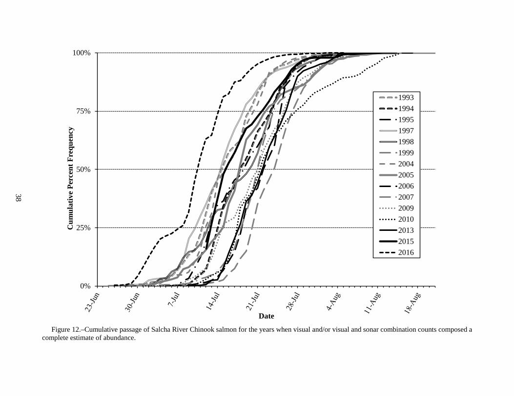
38
Figure 12.–Cumulative passage of Salcha River Chinook salmon for the years when visual and/or visual and sonar combination counts composed a
complete estimate of abundance.
0%
25%
50%
75%
100%
Cum
ulat
ive
Perc
ent F
requ
ency
Date
199319941995199719981999200420052006200720092010201320152016
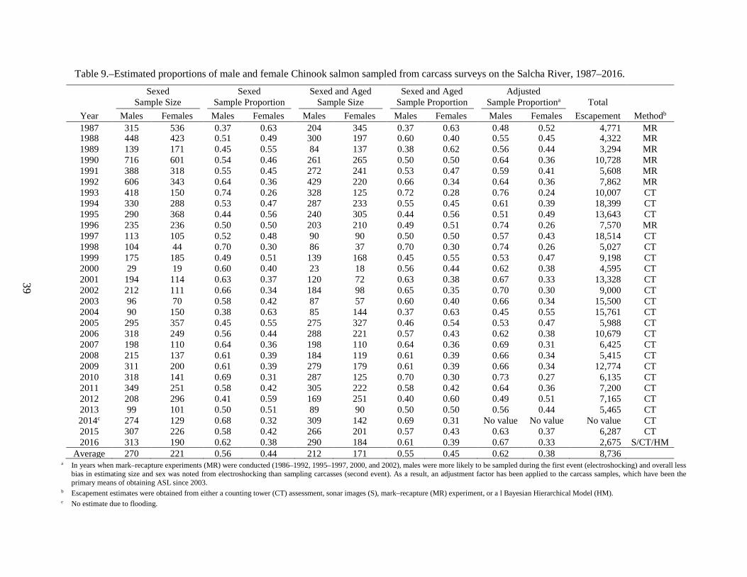
39
Table 9.–Estimated proportions of male and female Chinook salmon sampled from carcass surveys on the Salcha River, 1987–2016. Sexed Sexed Sexed and Aged Sexed and Aged Adjusted
Sample Size Sample Proportion Sample Size Sample Proportion Sample Proportiona Total
Year Males Females Males Females Males Females Males Females Males Females Escapement Methodb 1987 315 536 0.37 0.63 204 345 0.37 0.63 0.48 0.52 4,771 MR 1988 448 423 0.51 0.49 300 197 0.60 0.40 0.55 0.45 4,322 MR 1989 139 171 0.45 0.55 84 137 0.38 0.62 0.56 0.44 3,294 MR 1990 716 601 0.54 0.46 261 265 0.50 0.50 0.64 0.36 10,728 MR 1991 388 318 0.55 0.45 272 241 0.53 0.47 0.59 0.41 5,608 MR 1992 606 343 0.64 0.36 429 220 0.66 0.34 0.64 0.36 7,862 MR 1993 418 150 0.74 0.26 328 125 0.72 0.28 0.76 0.24 10,007 CT 1994 330 288 0.53 0.47 287 233 0.55 0.45 0.61 0.39 18,399 CT 1995 290 368 0.44 0.56 240 305 0.44 0.56 0.51 0.49 13,643 CT 1996 235 236 0.50 0.50 203 210 0.49 0.51 0.74 0.26 7,570 MR 1997 113 105 0.52 0.48 90 90 0.50 0.50 0.57 0.43 18,514 CT 1998 104 44 0.70 0.30 86 37 0.70 0.30 0.74 0.26 5,027 CT 1999 175 185 0.49 0.51 139 168 0.45 0.55 0.53 0.47 9,198 CT 2000 29 19 0.60 0.40 23 18 0.56 0.44 0.62 0.38 4,595 CT 2001 194 114 0.63 0.37 120 72 0.63 0.38 0.67 0.33 13,328 CT 2002 212 111 0.66 0.34 184 98 0.65 0.35 0.70 0.30 9,000 CT 2003 96 70 0.58 0.42 87 57 0.60 0.40 0.66 0.34 15,500 CT 2004 90 150 0.38 0.63 85 144 0.37 0.63 0.45 0.55 15,761 CT 2005 295 357 0.45 0.55 275 327 0.46 0.54 0.53 0.47 5,988 CT 2006 318 249 0.56 0.44 288 221 0.57 0.43 0.62 0.38 10,679 CT 2007 198 110 0.64 0.36 198 110 0.64 0.36 0.69 0.31 6,425 CT 2008 215 137 0.61 0.39 184 119 0.61 0.39 0.66 0.34 5,415 CT 2009 311 200 0.61 0.39 279 179 0.61 0.39 0.66 0.34 12,774 CT 2010 318 141 0.69 0.31 287 125 0.70 0.30 0.73 0.27 6,135 CT 2011 349 251 0.58 0.42 305 222 0.58 0.42 0.64 0.36 7,200 CT 2012 208 296 0.41 0.59 169 251 0.40 0.60 0.49 0.51 7,165 CT 2013 99 101 0.50 0.51 89 90 0.50 0.50 0.56 0.44 5,465 CT 2014c 274 129 0.68 0.32 309 142 0.69 0.31 No value No value No value CT 2015 307 226 0.58 0.42 266 201 0.57 0.43 0.63 0.37 6,287 CT 2016 313 190 0.62 0.38 290 184 0.61 0.39 0.67 0.33 2,675 S/CT/HM
Average 270 221 0.56 0.44 212 171 0.55 0.45 0.62 0.38 8,736 a In years when mark–recapture experiments (MR) were conducted (1986–1992, 1995–1997, 2000, and 2002), males were more likely to be sampled during the first event (electroshocking) and overall less
bias in estimating size and sex was noted from electroshocking than sampling carcasses (second event). As a result, an adjustment factor has been applied to the carcass samples, which have been the primary means of obtaining ASL since 2003.
b Escapement estimates were obtained from either a counting tower (CT) assessment, sonar images (S), mark–recapture (MR) experiment, or a l Bayesian Hierarchical Model (HM). c No estimate due to flooding.
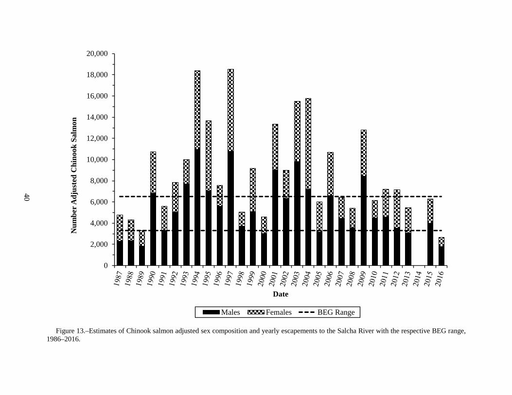
40
Figure 13.–Estimates of Chinook salmon adjusted sex composition and yearly escapements to the Salcha River with the respective BEG range,
1986–2016.
0
2,000
4,000
6,000
8,000
10,000
12,000
14,000
16,000
18,000
20,000
Num
ber A
djus
ted
Chi
nook
Sal
mon
Date
Males Females BEG Range
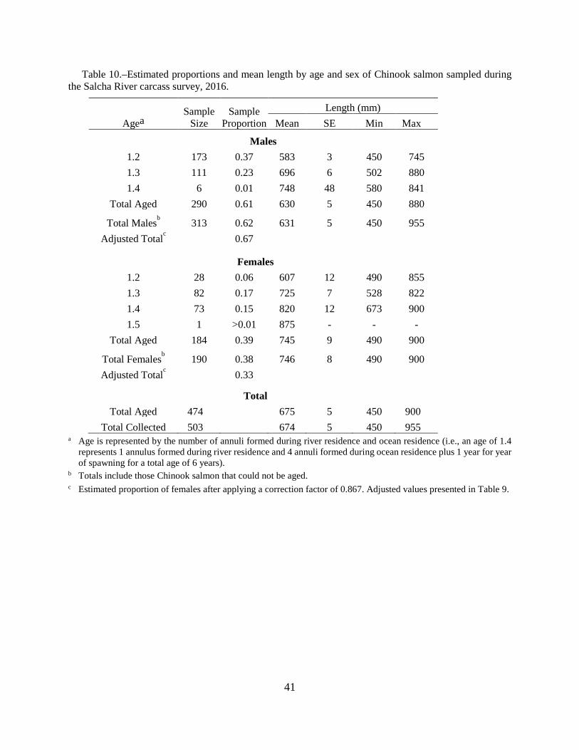
41
Table 10.–Estimated proportions and mean length by age and sex of Chinook salmon sampled during the Salcha River carcass survey, 2016.
Agea Sample
Size Sample
Proportion Length (mm)
Mean SE Min Max
Males 1.2 173 0.37 583 3 450 745 1.3 111 0.23 696 6 502 880 1.4 6 0.01 748 48 580 841
Total Aged 290 0.61 630 5 450 880
Total Malesb 313 0.62 631 5 450 955 Adjusted Totalc 0.67
Females 1.2 28 0.06 607 12 490 855 1.3 82 0.17 725 7 528 822 1.4 73 0.15 820 12 673 900 1.5 1 >0.01 875 - - -
Total Aged 184 0.39 745 9 490 900
Total Femalesb 190 0.38 746 8 490 900 Adjusted Totalc 0.33
Total Total Aged 474 675 5 450 900
Total Collected 503 674 5 450 955 a Age is represented by the number of annuli formed during river residence and ocean residence (i.e., an age of 1.4
represents 1 annulus formed during river residence and 4 annuli formed during ocean residence plus 1 year for year of spawning for a total age of 6 years).
b Totals include those Chinook salmon that could not be aged. c Estimated proportion of females after applying a correction factor of 0.867. Adjusted values presented in Table 9.
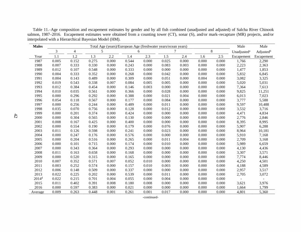
42
Table 11.–Age composition and escapement estimates by gender and by all fish combined (unadjusted and adjusted) of Salcha River Chinook salmon, 1987–2016. Escapement estimates were obtained from a counting tower (CT), sonar (S), and/or mark–recapture (MR) projects, and/or interpolated with a Hierarchical Bayesian Model (HM).
Males Total Age (years)/European Age (freshwater years/ocean years) Male Male
3 4 5 6 7 8 Unadjusteda Adjustedb Year 1.1 1.2 1.3 2.2 1.4 2.3 1.5 2.4 1.6 2.5 Escapement Escapement 1987 0.005 0.152 0.275 0.000 0.544 0.000 0.025 0.000 0.000 0.000 1,766 2,290 1988 0.007 0.333 0.330 0.000 0.243 0.000 0.083 0.003 0.000 0.000 2,223 2,363 1989 0.012 0.107 0.548 0.000 0.333 0.000 0.000 0.000 0.000 0.000 1,477 1,853 1990 0.004 0.333 0.352 0.000 0.268 0.000 0.042 0.000 0.000 0.000 5,832 6,845 1991 0.004 0.143 0.489 0.000 0.309 0.000 0.051 0.000 0.004 0.000 3,082 3,325 1992 0.019 0.543 0.338 0.007 0.084 0.005 0.005 0.000 0.000 0.000 5,020 5,031 1993 0.012 0.384 0.454 0.000 0.146 0.003 0.000 0.000 0.000 0.000 7,364 7,613 1994 0.010 0.035 0.561 0.000 0.366 0.000 0.028 0.000 0.000 0.000 9,825 11,251 1995 0.000 0.296 0.292 0.000 0.388 0.000 0.021 0.004 0.000 0.000 6,013 7,023 1996 0.054 0.118 0.567 0.000 0.177 0.000 0.084 0.000 0.000 0.000 3,777 5,588 1997 0.000 0.256 0.244 0.000 0.489 0.000 0.011 0.000 0.000 0.000 9,597 10,488 1998 0.035 0.070 0.756 0.000 0.128 0.000 0.012 0.000 0.000 0.000 3,532 3,716 1999 0.000 0.201 0.374 0.000 0.424 0.000 0.000 0.000 0.000 0.000 4,471 4,834 2000 0.000 0.304 0.565 0.000 0.130 0.000 0.000 0.000 0.000 0.000 2,776 2,846 2001 0.008 0.167 0.425 0.000 0.400 0.000 0.000 0.000 0.000 0.000 8,395 8,995 2002 0.000 0.554 0.190 0.000 0.179 0.000 0.076 0.000 0.000 0.000 5,907 6,288 2003 0.011 0.126 0.598 0.000 0.241 0.000 0.023 0.000 0.000 0.000 8,964 10,181 2004 0.000 0.247 0.176 0.000 0.576 0.000 0.000 0.000 0.000 0.000 5,910 7,168 2005 0.000 0.204 0.516 0.000 0.265 0.000 0.011 0.004 0.000 0.000 2,709 3,168 2006 0.000 0.101 0.715 0.000 0.174 0.000 0.010 0.000 0.000 0.000 5,989 6,659 2007 0.000 0.343 0.364 0.000 0.293 0.000 0.000 0.000 0.000 0.000 4,130 4,436 2008 0.011 0.163 0.658 0.000 0.168 0.000 0.000 0.000 0.000 0.000 3,307 3,571 2009 0.000 0.520 0.315 0.000 0.165 0.000 0.000 0.000 0.000 0.000 7,774 8,446 2010 0.007 0.352 0.571 0.007 0.052 0.010 0.000 0.000 0.000 0.000 4,250 4,501 2011 0.003 0.252 0.574 0.000 0.157 0.010 0.003 0.000 0.000 0.000 4,188 4,589 2012 0.006 0.148 0.509 0.000 0.337 0.000 0.000 0.000 0.000 0.000 2,957 3,517 2013 0.022 0.225 0.202 0.000 0.539 0.000 0.011 0.000 0.000 0.000 2,705 3,072 2014d 0.022 0.215 0.701 0.004 0.055 0.000 0.004 0.000 0.000 0.000 - - 2015 0.011 0.402 0.391 0.008 0.180 0.008 0.000 0.000 0.000 0.000 3,621 3,976 2016 0.000 0.597 0.383 0.000 0.021 0.000 0.000 0.000 0.000 0.000 1,664 1,799
Average 0.009 0.263 0.448 0.001 0.261 0.001 0.017 0.000 0.000 0.000 4,801 5,360 -continued-
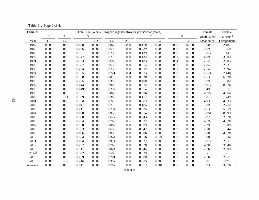
43
Table 11.–Page 2 of 4.
Females Total Age (years)/European Age (freshwater years/ocean years) Female Female
3 4 5 6 7 8 Unadjusteda Adjustedb Year 1.1 1.2 1.3 2.2 1.4 2.3 1.5 2.4 1.6 2.5 Escapement Escapement 1987 0.000 0.003 0.038 0.000 0.849 0.000 0.110 0.000 0.000 0.000 3,005 2,481 1988 0.000 0.005 0.066 0.000 0.690 0.000 0.239 0.000 0.000 0.000 2,099 1,959 1989 0.000 0.000 0.131 0.000 0.730 0.000 0.139 0.000 0.000 0.000 1,817 1,441 1990 0.000 0.008 0.147 0.000 0.713 0.000 0.132 0.000 0.000 0.000 4,896 3,883 1991 0.000 0.000 0.133 0.000 0.680 0.000 0.183 0.000 0.004 0.000 2,526 2,283 1992 0.000 0.005 0.327 0.000 0.650 0.000 0.014 0.005 0.000 0.000 2,842 2,831 1993 0.000 0.008 0.224 0.000 0.736 0.000 0.032 0.000 0.000 0.000 2,643 2,394 1994 0.000 0.017 0.185 0.000 0.721 0.004 0.073 0.000 0.000 0.000 8,574 7,148 1995 0.000 0.010 0.138 0.000 0.816 0.000 0.030 0.007 0.000 0.000 7,630 6,620 1996 0.000 0.005 0.205 0.000 0.390 0.000 0.400 0.000 0.000 0.000 3,793 1,982 1997 0.000 0.033 0.044 0.000 0.900 0.000 0.022 0.000 0.000 0.000 8,917 8,026 1998 0.000 0.000 0.649 0.000 0.297 0.000 0.054 0.000 0.000 0.000 1,495 1,311 1999 0.000 0.000 0.131 0.000 0.863 0.000 0.006 0.000 0.000 0.000 4,727 4,364 2000 0.000 0.111 0.389 0.000 0.389 0.000 0.111 0.000 0.000 0.000 1,819 1,749 2001 0.000 0.000 0.194 0.000 0.722 0.000 0.083 0.000 0.000 0.000 4,933 4,333 2002 0.000 0.000 0.041 0.000 0.776 0.000 0.184 0.000 0.000 0.000 3,093 2,712 2003 0.000 0.000 0.211 0.000 0.754 0.000 0.035 0.000 0.000 0.000 6,536 5,319 2004 0.000 0.000 0.028 0.000 0.958 0.000 0.014 0.000 0.000 0.000 9,851 8,593 2005 0.000 0.000 0.330 0.000 0.627 0.000 0.043 0.000 0.000 0.000 3,279 2,820 2006 0.000 0.000 0.204 0.000 0.760 0.005 0.032 0.000 0.000 0.000 4,690 4,020 2007 0.000 0.009 0.100 0.000 0.882 0.000 0.009 0.000 0.000 0.000 2,295 1,989 2008 0.000 0.000 0.303 0.000 0.655 0.000 0.042 0.000 0.000 0.000 2,108 1,844 2009 0.000 0.000 0.056 0.000 0.939 0.000 0.006 0.000 0.000 0.000 5,000 4,328 2010 0.000 0.032 0.584 0.000 0.344 0.000 0.016 0.024 0.000 0.000 1,885 1,634 2011 0.000 0.000 0.054 0.000 0.914 0.000 0.032 0.000 0.000 0.000 3,012 2,611 2012 0.000 0.000 0.207 0.000 0.765 0.000 0.028 0.000 0.000 0.000 4,208 3,648 2013 0.000 0.000 0.111 0.000 0.844 0.000 0.044 0.000 0.000 0.000 2,760 2,393 2014d 0.000 0.000 0.372 0.000 0.589 0.000 0.039 0.000 0.000 0.000 - - 2015 0.000 0.000 0.299 0.000 0.701 0.000 0.000 0.000 0.000 0.000 2,666 2,311 2016 0.000 0.152 0.446 0.000 0.397 0.000 0.005 0.000 0.000 0.000 1,010 876
Average 0.000 0.013 0.211 0.000 0.702 0.000 0.072 0.001 0.000 0.000 3,935 3,376 -continued-
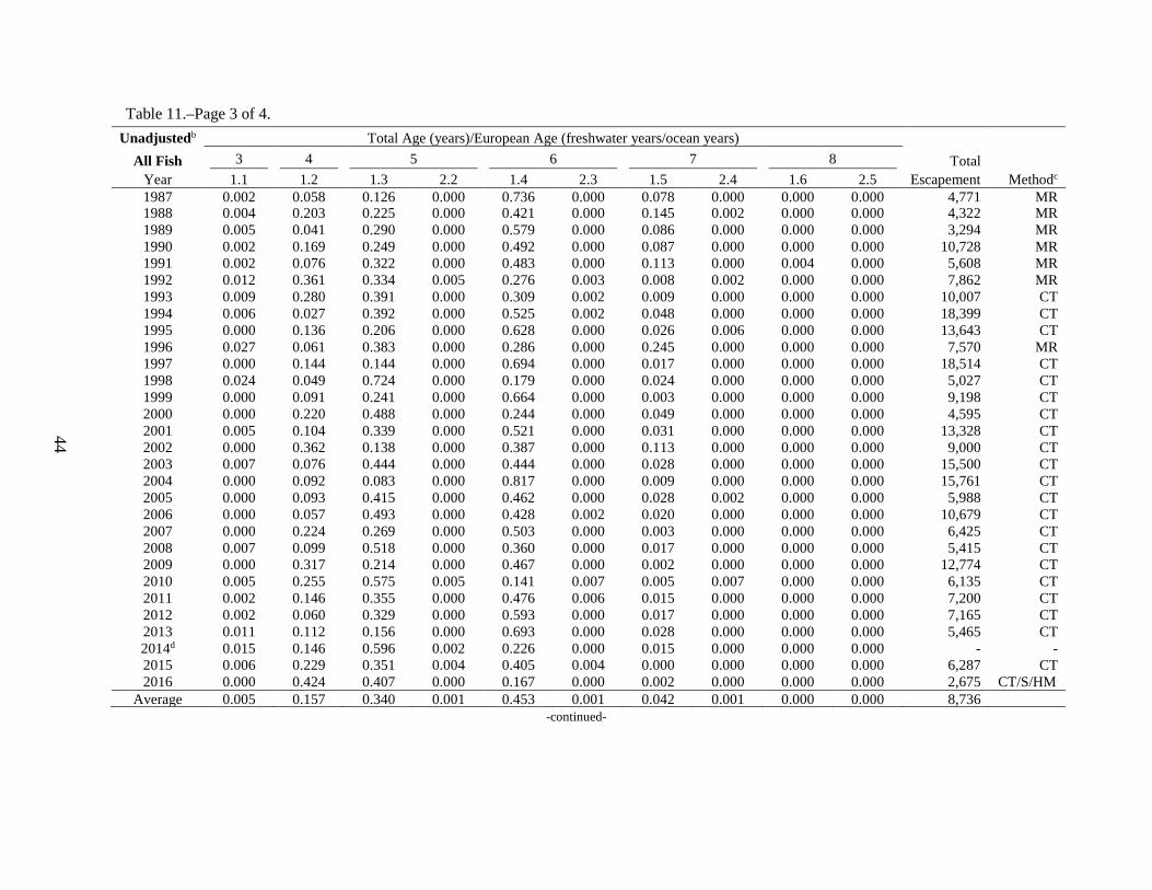
44
Table 11.–Page 3 of 4. Unadjustedb Total Age (years)/European Age (freshwater years/ocean years)
All Fish 3 4 5 6 7 8 Total Year 1.1 1.2 1.3 2.2 1.4 2.3 1.5 2.4 1.6 2.5 Escapement Methodc
1987 0.002 0.058 0.126 0.000 0.736 0.000 0.078 0.000 0.000 0.000 4,771 MR 1988 0.004 0.203 0.225 0.000 0.421 0.000 0.145 0.002 0.000 0.000 4,322 MR 1989 0.005 0.041 0.290 0.000 0.579 0.000 0.086 0.000 0.000 0.000 3,294 MR 1990 0.002 0.169 0.249 0.000 0.492 0.000 0.087 0.000 0.000 0.000 10,728 MR 1991 0.002 0.076 0.322 0.000 0.483 0.000 0.113 0.000 0.004 0.000 5,608 MR 1992 0.012 0.361 0.334 0.005 0.276 0.003 0.008 0.002 0.000 0.000 7,862 MR 1993 0.009 0.280 0.391 0.000 0.309 0.002 0.009 0.000 0.000 0.000 10,007 CT 1994 0.006 0.027 0.392 0.000 0.525 0.002 0.048 0.000 0.000 0.000 18,399 CT 1995 0.000 0.136 0.206 0.000 0.628 0.000 0.026 0.006 0.000 0.000 13,643 CT 1996 0.027 0.061 0.383 0.000 0.286 0.000 0.245 0.000 0.000 0.000 7,570 MR 1997 0.000 0.144 0.144 0.000 0.694 0.000 0.017 0.000 0.000 0.000 18,514 CT 1998 0.024 0.049 0.724 0.000 0.179 0.000 0.024 0.000 0.000 0.000 5,027 CT 1999 0.000 0.091 0.241 0.000 0.664 0.000 0.003 0.000 0.000 0.000 9,198 CT 2000 0.000 0.220 0.488 0.000 0.244 0.000 0.049 0.000 0.000 0.000 4,595 CT 2001 0.005 0.104 0.339 0.000 0.521 0.000 0.031 0.000 0.000 0.000 13,328 CT 2002 0.000 0.362 0.138 0.000 0.387 0.000 0.113 0.000 0.000 0.000 9,000 CT 2003 0.007 0.076 0.444 0.000 0.444 0.000 0.028 0.000 0.000 0.000 15,500 CT 2004 0.000 0.092 0.083 0.000 0.817 0.000 0.009 0.000 0.000 0.000 15,761 CT 2005 0.000 0.093 0.415 0.000 0.462 0.000 0.028 0.002 0.000 0.000 5,988 CT 2006 0.000 0.057 0.493 0.000 0.428 0.002 0.020 0.000 0.000 0.000 10,679 CT 2007 0.000 0.224 0.269 0.000 0.503 0.000 0.003 0.000 0.000 0.000 6,425 CT 2008 0.007 0.099 0.518 0.000 0.360 0.000 0.017 0.000 0.000 0.000 5,415 CT 2009 0.000 0.317 0.214 0.000 0.467 0.000 0.002 0.000 0.000 0.000 12,774 CT 2010 0.005 0.255 0.575 0.005 0.141 0.007 0.005 0.007 0.000 0.000 6,135 CT 2011 0.002 0.146 0.355 0.000 0.476 0.006 0.015 0.000 0.000 0.000 7,200 CT 2012 0.002 0.060 0.329 0.000 0.593 0.000 0.017 0.000 0.000 0.000 7,165 CT 2013 0.011 0.112 0.156 0.000 0.693 0.000 0.028 0.000 0.000 0.000 5,465 CT 2014d 0.015 0.146 0.596 0.002 0.226 0.000 0.015 0.000 0.000 0.000 - - 2015 0.006 0.229 0.351 0.004 0.405 0.004 0.000 0.000 0.000 0.000 6,287 CT 2016 0.000 0.424 0.407 0.000 0.167 0.000 0.002 0.000 0.000 0.000 2,675 CT/S/HM
Average 0.005 0.157 0.340 0.001 0.453 0.001 0.042 0.001 0.000 0.000 8,736 -continued-
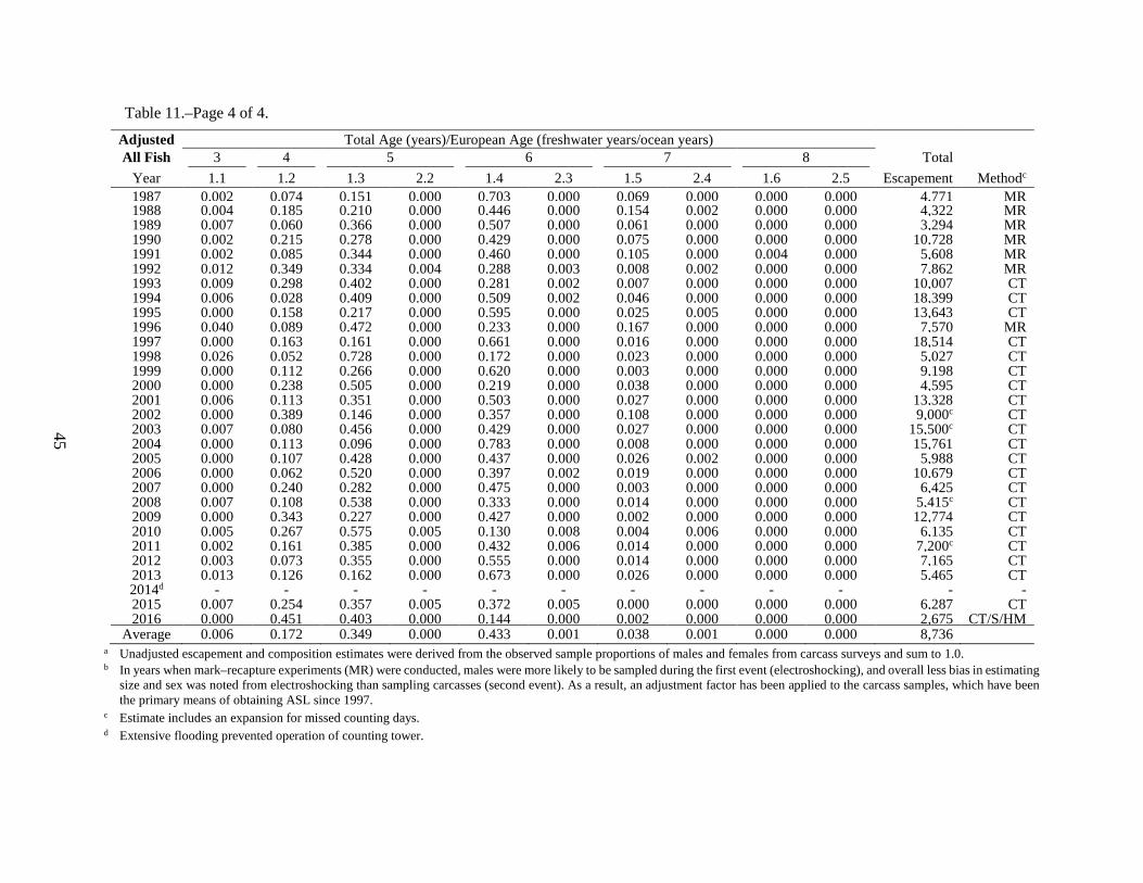
45
Table 11.–Page 4 of 4. Adjusted Total Age (years)/European Age (freshwater years/ocean years) All Fish 3 4 5 6 7 8 Total
Year 1.1 1.2 1.3 2.2 1.4 2.3 1.5 2.4 1.6 2.5 Escapement Methodc
1987 0.002 0.074 0.151 0.000 0.703 0.000 0.069 0.000 0.000 0.000 4,771 MR 1988 0.004 0.185 0.210 0.000 0.446 0.000 0.154 0.002 0.000 0.000 4,322 MR 1989 0.007 0.060 0.366 0.000 0.507 0.000 0.061 0.000 0.000 0.000 3,294 MR 1990 0.002 0.215 0.278 0.000 0.429 0.000 0.075 0.000 0.000 0.000 10,728 MR 1991 0.002 0.085 0.344 0.000 0.460 0.000 0.105 0.000 0.004 0.000 5,608 MR 1992 0.012 0.349 0.334 0.004 0.288 0.003 0.008 0.002 0.000 0.000 7,862 MR 1993 0.009 0.298 0.402 0.000 0.281 0.002 0.007 0.000 0.000 0.000 10,007 CT 1994 0.006 0.028 0.409 0.000 0.509 0.002 0.046 0.000 0.000 0.000 18,399 CT 1995 0.000 0.158 0.217 0.000 0.595 0.000 0.025 0.005 0.000 0.000 13,643 CT 1996 0.040 0.089 0.472 0.000 0.233 0.000 0.167 0.000 0.000 0.000 7,570 MR 1997 0.000 0.163 0.161 0.000 0.661 0.000 0.016 0.000 0.000 0.000 18,514 CT 1998 0.026 0.052 0.728 0.000 0.172 0.000 0.023 0.000 0.000 0.000 5,027 CT 1999 0.000 0.112 0.266 0.000 0.620 0.000 0.003 0.000 0.000 0.000 9,198 CT 2000 0.000 0.238 0.505 0.000 0.219 0.000 0.038 0.000 0.000 0.000 4,595 CT 2001 0.006 0.113 0.351 0.000 0.503 0.000 0.027 0.000 0.000 0.000 13,328 CT 2002 0.000 0.389 0.146 0.000 0.357 0.000 0.108 0.000 0.000 0.000 9,000c CT 2003 0.007 0.080 0.456 0.000 0.429 0.000 0.027 0.000 0.000 0.000 15,500c CT 2004 0.000 0.113 0.096 0.000 0.783 0.000 0.008 0.000 0.000 0.000 15,761 CT 2005 0.000 0.107 0.428 0.000 0.437 0.000 0.026 0.002 0.000 0.000 5,988 CT 2006 0.000 0.062 0.520 0.000 0.397 0.002 0.019 0.000 0.000 0.000 10,679 CT 2007 0.000 0.240 0.282 0.000 0.475 0.000 0.003 0.000 0.000 0.000 6,425 CT 2008 0.007 0.108 0.538 0.000 0.333 0.000 0.014 0.000 0.000 0.000 5,415c CT 2009 0.000 0.343 0.227 0.000 0.427 0.000 0.002 0.000 0.000 0.000 12,774 CT 2010 0.005 0.267 0.575 0.005 0.130 0.008 0.004 0.006 0.000 0.000 6,135 CT 2011 0.002 0.161 0.385 0.000 0.432 0.006 0.014 0.000 0.000 0.000 7,200c CT 2012 0.003 0.073 0.355 0.000 0.555 0.000 0.014 0.000 0.000 0.000 7,165 CT 2013 0.013 0.126 0.162 0.000 0.673 0.000 0.026 0.000 0.000 0.000 5,465 CT 2014d - - - - - - - - - - - - 2015 0.007 0.254 0.357 0.005 0.372 0.005 0.000 0.000 0.000 0.000 6,287 CT 2016 0.000 0.451 0.403 0.000 0.144 0.000 0.002 0.000 0.000 0.000 2,675 CT/S/HM
Average 0.006 0.172 0.349 0.000 0.433 0.001 0.038 0.001 0.000 0.000 8,736
a Unadjusted escapement and composition estimates were derived from the observed sample proportions of males and females from carcass surveys and sum to 1.0. b In years when mark–recapture experiments (MR) were conducted, males were more likely to be sampled during the first event (electroshocking), and overall less bias in estimating
size and sex was noted from electroshocking than sampling carcasses (second event). As a result, an adjustment factor has been applied to the carcass samples, which have been the primary means of obtaining ASL since 1997.
c Estimate includes an expansion for missed counting days. d Extensive flooding prevented operation of counting tower.
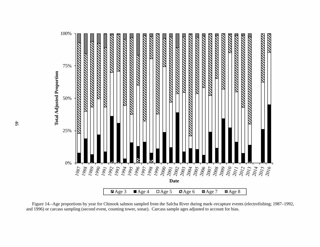
46
Figure 14.–Age proportions by year for Chinook salmon sampled from the Salcha River during mark–recapture events (electrofishing; 1987–1992,
and 1996) or carcass sampling (second event, counting tower, sonar). Carcass sample ages adjusted to account for bias.
0%
25%
50%
75%
100%
Tota
l Adj
uste
d Pr
opor
tion
Date
Age 3 Age 4 Age 5 Age 6 Age 7 Age 8
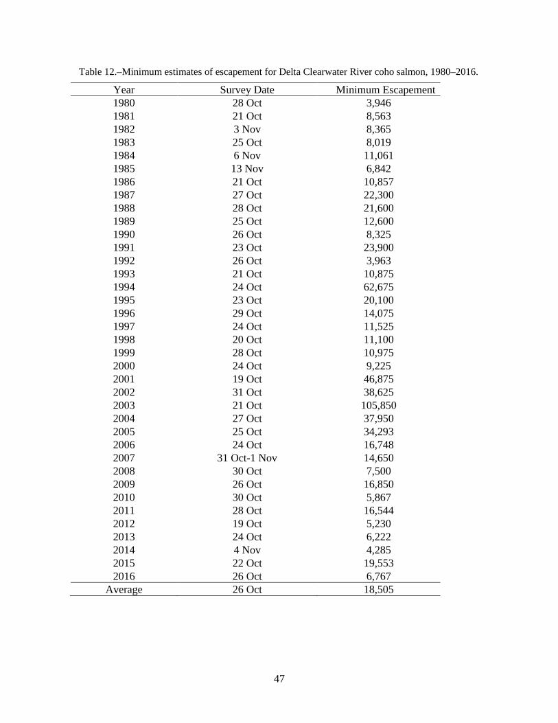
47
Table 12.–Minimum estimates of escapement for Delta Clearwater River coho salmon, 1980–2016.
Year Survey Date Minimum Escapement 1980 28 Oct 3,946 1981 21 Oct 8,563 1982 3 Nov 8,365 1983 25 Oct 8,019 1984 6 Nov 11,061 1985 13 Nov 6,842 1986 21 Oct 10,857 1987 27 Oct 22,300 1988 28 Oct 21,600 1989 25 Oct 12,600 1990 26 Oct 8,325 1991 23 Oct 23,900 1992 26 Oct 3,963 1993 21 Oct 10,875 1994 24 Oct 62,675 1995 23 Oct 20,100 1996 29 Oct 14,075 1997 24 Oct 11,525 1998 20 Oct 11,100 1999 28 Oct 10,975 2000 24 Oct 9,225 2001 19 Oct 46,875 2002 31 Oct 38,625 2003 21 Oct 105,850 2004 27 Oct 37,950 2005 25 Oct 34,293 2006 24 Oct 16,748 2007 31 Oct-1 Nov 14,650 2008 30 Oct 7,500 2009 26 Oct 16,850 2010 30 Oct 5,867 2011 28 Oct 16,544 2012 19 Oct 5,230 2013 24 Oct 6,222 2014 4 Nov 4,285 2015 22 Oct 19,553 2016 26 Oct 6,767
Average 26 Oct 18,505
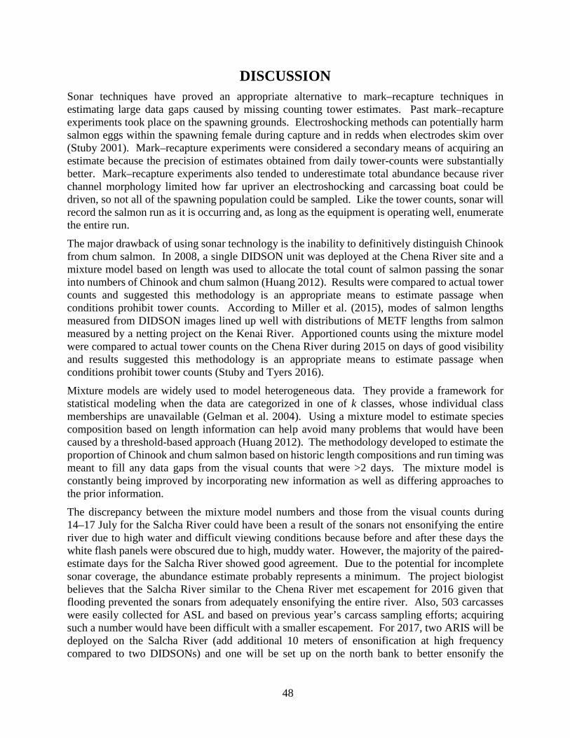
48
DISCUSSION Sonar techniques have proved an appropriate alternative to mark–recapture techniques in estimating large data gaps caused by missing counting tower estimates. Past mark–recapture experiments took place on the spawning grounds. Electroshocking methods can potentially harm salmon eggs within the spawning female during capture and in redds when electrodes skim over (Stuby 2001). Mark–recapture experiments were considered a secondary means of acquiring an estimate because the precision of estimates obtained from daily tower-counts were substantially better. Mark–recapture experiments also tended to underestimate total abundance because river channel morphology limited how far upriver an electroshocking and carcassing boat could be driven, so not all of the spawning population could be sampled. Like the tower counts, sonar will record the salmon run as it is occurring and, as long as the equipment is operating well, enumerate the entire run.
The major drawback of using sonar technology is the inability to definitively distinguish Chinook from chum salmon. In 2008, a single DIDSON unit was deployed at the Chena River site and a mixture model based on length was used to allocate the total count of salmon passing the sonar into numbers of Chinook and chum salmon (Huang 2012). Results were compared to actual tower counts and suggested this methodology is an appropriate means to estimate passage when conditions prohibit tower counts. According to Miller et al. (2015), modes of salmon lengths measured from DIDSON images lined up well with distributions of METF lengths from salmon measured by a netting project on the Kenai River. Apportioned counts using the mixture model were compared to actual tower counts on the Chena River during 2015 on days of good visibility and results suggested this methodology is an appropriate means to estimate passage when conditions prohibit tower counts (Stuby and Tyers 2016).
Mixture models are widely used to model heterogeneous data. They provide a framework for statistical modeling when the data are categorized in one of k classes, whose individual class memberships are unavailable (Gelman et al. 2004). Using a mixture model to estimate species composition based on length information can help avoid many problems that would have been caused by a threshold-based approach (Huang 2012). The methodology developed to estimate the proportion of Chinook and chum salmon based on historic length compositions and run timing was meant to fill any data gaps from the visual counts that were >2 days. The mixture model is constantly being improved by incorporating new information as well as differing approaches to the prior information.
The discrepancy between the mixture model numbers and those from the visual counts during 14–17 July for the Salcha River could have been a result of the sonars not ensonifying the entire river due to high water and difficult viewing conditions because before and after these days the white flash panels were obscured due to high, muddy water. However, the majority of the paired-estimate days for the Salcha River showed good agreement. Due to the potential for incomplete sonar coverage, the abundance estimate probably represents a minimum. The project biologist believes that the Salcha River similar to the Chena River met escapement for 2016 given that flooding prevented the sonars from adequately ensonifying the entire river. Also, 503 carcasses were easily collected for ASL and based on previous year’s carcass sampling efforts; acquiring such a number would have been difficult with a smaller escapement. For 2017, two ARIS will be deployed on the Salcha River (add additional 10 meters of ensonification at high frequency compared to two DIDSONs) and one will be set up on the north bank to better ensonify the

49
thalweg. The counting tower will also be moved to the north bank for better visual reception of salmon passing through the thalweg.
The Bayesian hierarchical model used for interpolation of daily counts gave biologically reasonable results when visual counts and sonar data were unavailable. However, daily estimates had a great deal of associated variance, and were conditional on the assumption that the functional form of the run-timing profile was expressed correctly.
Chinook salmon run-timing for the Salcha and Chena rivers have shown similarities over the years. This is not too surprising since both are tributaries of the Tanana River and are in relative proximity to each other and share headwaters. One of the biggest factors affecting run-timing is date of river breakup in the Yukon and Tanana rivers. Ice breakup at the mouth of the Yukon River occurred on 3 May 2016 which was more than 3 weeks earlier than the average break up date of 25 May based on the years 1961–2015 (JTC 2017). The first subsistence caught Chinook salmon was harvested on 23 May, one week earlier than the average date of 31 May (JTC 2017). During past years when river breakups were comparatively late, the first fish recorded by the counting towers and sonars were similarly late. However, over the years it has been observed that no matter when the Chinook salmon arrive to their spawning destinations, sampling for post-spawning carcasses has always occurred during the same time period of very late July to mid-August. Towards the end of carcass sampling, salmon become hard to locate as most have decomposed.
For 2014 and 2015, the Chena and Salcha rivers Chinook salmon sport fishery was closed early in the season because Lower Yukon River preseason forecasts and early season indicators suggested that the Chinook salmon runs were not projected to meet minimum escapements (JTC 2015). There was a sport fishery for these interior rivers during 2016; however, due to flooding, harvest values are anticipated to be low. Restrictions were placed on subsistence, commercial, and sport users in the Yukon River (JTC 2017). It is likely that the escapement goals were met during the past 3 seasons because of all the restrictions placed on Chinook salmon fisheries in the Yukon and Tanana River drainages.
In general, greater proportions of large females are important for overall stock health in Chinook salmon. Larger females generally have larger and more numerous eggs (Wertheimer, et al. 2004), larger eggs produce larger juveniles, which tend to have higher survival rates (Quinn 2005). Since size and age-at-maturity are heritable (Ferrari 2004), selection for smaller sizes leads to a feedback loop in which younger and smaller adults produce offspring that mature earlier at smaller sizes (Lewis et al. 2015). Typically, there are more males than females in Chena and Salcha river composition estimates. Males vary more in size and maturity than females, and for most Chinook salmon populations the average male will be smaller than the average female (Quinn 2005). In 2015, the female population was larger than what has been noted in the past 5 years. However, the opposite occurred during 2016, with one of the smallest female proportion estimate in recent years. This dichotomy was also seen from Upper Yukon River drainage escapement projects such as at Eagle (33% female) and Porcupine River sonar in Canada. For both projects because of concern over the lower number of females observed, precautionary approaches with a conservative harvest, small gill net mesh sizes, and release of females were implemented and maintained throughout the season.
For Chinook salmon enumeration projects below the Tanana River, female proportion was estimated at 45% to 50% (JTC 2017). Nevertheless, in the Lower and Middle Yukon River, gillnet mesh size was restricted as Howard and Evenson (2010) noticed that as mesh size increases, the
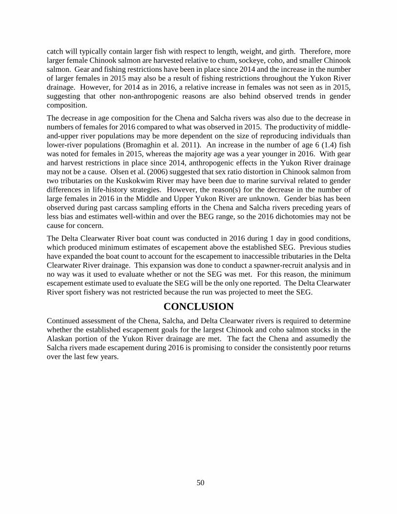
50
catch will typically contain larger fish with respect to length, weight, and girth. Therefore, more larger female Chinook salmon are harvested relative to chum, sockeye, coho, and smaller Chinook salmon. Gear and fishing restrictions have been in place since 2014 and the increase in the number of larger females in 2015 may also be a result of fishing restrictions throughout the Yukon River drainage. However, for 2014 as in 2016, a relative increase in females was not seen as in 2015, suggesting that other non-anthropogenic reasons are also behind observed trends in gender composition.
The decrease in age composition for the Chena and Salcha rivers was also due to the decrease in numbers of females for 2016 compared to what was observed in 2015. The productivity of middle-and-upper river populations may be more dependent on the size of reproducing individuals than lower-river populations (Bromaghin et al. 2011). An increase in the number of age 6 (1.4) fish was noted for females in 2015, whereas the majority age was a year younger in 2016. With gear and harvest restrictions in place since 2014, anthropogenic effects in the Yukon River drainage may not be a cause. Olsen et al. (2006) suggested that sex ratio distortion in Chinook salmon from two tributaries on the Kuskokwim River may have been due to marine survival related to gender differences in life-history strategies. However, the reason(s) for the decrease in the number of large females in 2016 in the Middle and Upper Yukon River are unknown. Gender bias has been observed during past carcass sampling efforts in the Chena and Salcha rivers preceding years of less bias and estimates well-within and over the BEG range, so the 2016 dichotomies may not be cause for concern.
The Delta Clearwater River boat count was conducted in 2016 during 1 day in good conditions, which produced minimum estimates of escapement above the established SEG. Previous studies have expanded the boat count to account for the escapement to inaccessible tributaries in the Delta Clearwater River drainage. This expansion was done to conduct a spawner-recruit analysis and in no way was it used to evaluate whether or not the SEG was met. For this reason, the minimum escapement estimate used to evaluate the SEG will be the only one reported. The Delta Clearwater River sport fishery was not restricted because the run was projected to meet the SEG.
CONCLUSION Continued assessment of the Chena, Salcha, and Delta Clearwater rivers is required to determine whether the established escapement goals for the largest Chinook and coho salmon stocks in the Alaskan portion of the Yukon River drainage are met. The fact the Chena and assumedly the Salcha rivers made escapement during 2016 is promising to consider the consistently poor returns over the last few years.

51
ACKNOWLEDGEMENTS The author would like to thank the following ADF&G Sport Fish staff who made the 2016 Chena and Salcha rivers counting towers/sonar sites a success: crew leaders Virgil Davis, Chad Bear, Loren St. Amand, and Allison Matter; and the counting and sonar crews: Carmen Daggett, Brett George, Matt Stoller, Eric Nakalsky, Kipp Wilkinson, Mary Webb, Quinn Evenson, and David Spencer. Thanks to the assistant area manager, Brandy Baker, and field technician Ellie Mason, for performing the annual Delta Clearwater River coho salmon counts. Allison Matter processed all of the Chinook salmon scales. Anchorage Commercial Fisheries staff aged the Chinook salmon scale samples. James Savereide helped with counting tower and sonar set up, project design, gave valuable advice, and along with Rachael Kvapil, edited and prepared the final report. The U.S. Army Corps of Engineers provided access to the Moose Creek Dam. The Alaska Sustainable Salmon Fund (AKSSF) is funding the Chena River counting tower through 2018. Yukon River Salmon Research and Management Fund (USFWS) funded operation of the Salcha River in 2016. The coho salmon counts are annually funded through ADF&G base funds.
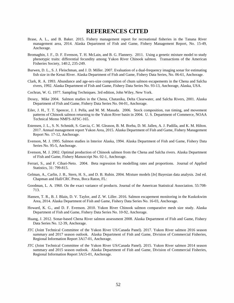
52
REFERENCES CITED Brase, A. L., and B. Baker. 2015. Fishery management report for recreational fisheries in the Tanana River
management area, 2014. Alaska Department of Fish and Game, Fishery Management Report, No. 15-49, Anchorage.
Bromaghin, J. F., D. F. Evenson, T. H. McLain, and B. G. Flannery. 2011. Using a genetic mixture model to study phenotypic traits: differential fecundity among Yukon River Chinook salmon. Transactions of the American Fisheries Society, 140:2, 235-249.
Burwen, D. L., S. J. Fleischman, and J. D. Miller. 2007. Evaluation of a dual-frequency imaging sonar for estimating fish size in the Kenai River. Alaska Department of Fish and Game, Fishery Data Series, No. 06-61, Anchorage.
Clark, R. A. 1993. Abundance and age-sex-size composition of chum salmon escapements in the Chena and Salcha rivers, 1992. Alaska Department of Fish and Game, Fishery Data Series No. 93-13, Anchorage, Alaska, USA.
Cochran, W. G. 1977. Sampling Techniques. 3rd edition, John Wiley, New York.
Doxey, Mike 2004. Salmon studies in the Chena, Chatanika, Delta Clearwater, and Salcha Rivers, 2001. Alaska Department of Fish and Game, Fishery Data Series No. 04-01, Anchorage.
Eiler, J. H., T. T. Spencer, J. J. Pella, and M. M. Masuda. 2006. Stock composition, run timing, and movement patterns of Chinook salmon returning to the Yukon River basin in 2004. U. S. Department of Commerce, NOAA Technical Memo NMFS-AFSC-165.
Estensen, J. L., S. N. Schmidt, S. Garcia, C. M. Gleason, B. M. Borba, D. M. Jallen, A. J. Padilla, and K. M. Hilton. 2017. Annual management report Yukon Area, 2015. Alaska Department of Fish and Game, Fishery Management Report No. 17-12, Anchorage.
Evenson, M. J. 1995. Salmon studies in Interior Alaska, 1994. Alaska Department of Fish and Game, Fishery Data Series No. 95-5, Anchorage.
Evenson, M. J. 2002. Optimal production of Chinook salmon from the Chena and Salcha rivers. Alaska Department of Fish and Game, Fishery Manuscript No. 02-1, Anchorage.
Ferrari, S., and F. Cibari-Neto. 2004. Beta regression for modelling rates and proportions. Journal of Applied Statistics, 31: 799-815.
Gelman, A., Carlin, J. B., Stern, H. S., and D. B. Rubin. 2004. Mixture models [In] Bayesian data analysis. 2nd ed. Chapman and Hall/CRC Press, Boca Raton, FL:
Goodman, L. A. 1960. On the exact variance of products. Journal of the American Statistical Association. 55:708-713.
Hansen, T. R., B. J. Blain, D. V. Taylor, and Z. W. Liller. 2016. Salmon escapement monitoring in the Kuskokwim Area, 2014. Alaska Department of Fish and Game, Fishery Data Series No. 16-03, Anchorage.
Howard, K. G., and D. F. Evenson. 2010. Yukon River Chinook salmon comparative mesh size study. Alaska Department of Fish and Game, Fishery Data Series No. 10-92, Anchorage.
Huang, J. 2012. Sonar-based Chena River salmon assessment 2008. Alaska Department of Fish and Game, Fishery Data Series No. 12-39, Anchorage.
JTC (Joint Technical Committee of the Yukon River US/Canada Panel). 2017. Yukon River salmon 2016 season summary and 2017 season outlook. Alaska Department of Fish and Game, Division of Commercial Fisheries, Regional Information Report 3A17-01, Anchorage.
JTC (Joint Technical Committee of the Yukon River US/Canada Panel). 2015. Yukon River salmon 2014 season summary and 2015 season outlook. Alaska Department of Fish and Game, Division of Commercial Fisheries, Regional Information Report 3A15-01, Anchorage.
53
REFERENCES CITED (Continued) Jennings, G. B., K. Sundet, and A. E. Bingham. 2011a. Estimates of participation, catch and harvest in Alaska sport
fisheries during 2009. Alaska Department of Fish and Game, Fishery Data Series No. 11-45, Anchorage.
Jennings, G. B., K. Sundet, and A. E. Bingham. 2011b. Estimates of participation, catch and harvest in Alaska sport fisheries during 2010. Alaska Department of Fish and Game, Fishery Data Series No. 11-60, Anchorage.
Jennings, G. B., K. Sundet, and A. E. Bingham. 2015. Estimates of participation, catch and harvest in Alaska sport fisheries during 2011. Alaska Department of Fish and Game, Fishery Data Series No. 15-04, Anchorage.
Lewis B., Grant W. S., Brenner R. E., Hamazaki T. 2015. Changes in size and age of Chinook Salmon Oncorhynchus tshawytscha returning to Alaska. PLoS ONE 10(6): e0130184. doi:10.1371/ journal.pone.0130184
Miller, J. D., D. L. Burwen, and S. J. Fleischman. 2015. Estimates of Chinook salmon passage in the Kenai River at river mile 8.6 using dual-frequency identification sonar, 2012. Alaska Department of Fish and Game, Fishery Data Series No. 15-09, Anchorage.
Mosher, K. H. 1969. Identification of Pacific salmon and steelhead trout by scale characteristics. United States Department of the Interior, U.S. Fish and Wildlife Service, Bureau of Commercial Fisheries, Washington, D.C., Circular 317.
Olsen, J. B., and S. J. Miller, K. Harper, J. J. Nagler, and J. K. Wenburg. 2005. Contrasting sex ratios in juvenile and adult Chinook salmon Oncorhynchus tshawytscha (Walbaum) from south-west Alaska: sex reversal or differential survival? Journal of Fish Biology, 69 (Supplement A), 140-144.
Parker, J. F. 2009. Fishery management report for sport fisheries in the Upper Tanana River drainage in 2008. Alaska Department of Fish and Game, Fishery Management Report No. 09-47, Anchorage.
Pfisterer, C. 2010. Echotastic 2.0 user manual. Alaska Department of Fish and Game, Fairbanks Alaska.
Plummer, M. 2003. JAGS: A program for analysis of Bayesian graphical models using Gibbs Sampling
Quinn, T. P. 2005. The behavior and ecology of Pacific salmon & trout. American Fisheries Society, University of Washington Press.
R Core Team. 2014. R: a language and environment for statistical computing. R Foundation for Statistical Computing, Vienna, Austria. www.R-project.org/.
Romberg, W. J., G. B. Jennings, K. Sundet, and A. E. Bingham. In prep. Estimates of participation, catch and harvest in Alaska sport fisheries during 2012. Alaska Department of Fish and Game, Fishery Data Series, Anchorage.
Stuby, L., and M. Tyers. 2016. Chinook salmon escapement in the Chena, Salcha, and Goodpaster rivers and coho salmon escapement in the Delta Clearwater River
Stuby, L. 2001. Salmon studies in interior Alaska, 2000. Alaska Department of Fish and Game, Fishery Data Series No. 01-24, Anchorage.
Su, Y. and Yajima, M. 2015. R2jags: A package for running jags from R. R package version 0.05-0.01. http://CRAN.R-project.org/package=R2jags.
Taras, B. D., and D. R. Sarafin. 2005. Chinook salmon escapement in the Gulkana River, 2002. Alaska Department of Fish and Game, Fishery Data Series No. 05-02, Anchorage.
Thompson, S. K. 1987. Sample size for estimating multinomial proportions. The American Statistician, 41:42-46.
Welander, A. D. 1940. A study of the development of the scale of the Chinook salmon (Oncorhynchus tshawytscha). Master’s thesis, University of Washington, Seattle.
Wertheimer, A. C., W. R. Heard, J. M. Maselko, and J. M. Smoker. 2004. Relationship of size at return with environmental variation, hatchery production, and productivity of wild pink salmon in Prince William Sound, Alaska: does size matter? Reviews in Fish Biology and Fisheries, 14: 321-334.
Wolter, K. M. 1985. Introduction to variance estimation. Springer-Verlag, New York.

54

55
APPENDIX A:
JAGS CODE OF MIXTURE MODEL

56
Appendix A1.–JAGS code of mixture model.
model { for(i in 1:n.fish) {
L.mm.D[i] ~ dnorm(muL[i],precL)
muL[i] <- betaD0[sonar[i]] + betaD1[sonar[i]]*L.mm.act[i]
L.mm.act[i] ~ dnorm(mu[i],tau[i])
mu[i] <- lambda[species[i],sex[i],river[i]]
tau[i] <- prec[species[i],sex[i],river[i]]
species[i] ~ dcat(ps[i,1:2])
sex[i] ~ dcat(psex[species[i],1:2])
logit(pi[i]) <- b0[river[i]]+b1[river[i]]*day[i]
alpha.inf[i,1] <- pi[i]
alpha.inf[i,2] <- (1-pi[i])
ps[i,1:2] ~ ddirch(alpha.inf[i,1:2])
}
## priors for sonar/actual length regression
# informed from Burwen tethered-fish experiment results
betaD0[1] ~ dnorm(44.81988,precbD0)
betaD1[1] ~ dnorm(0.87156,precbD1)
betaD0[2] ~ dnorm(44.81988,precbD0)
betaD1[2] ~ dnorm(0.87156,precbD1)
precbD0 <- 1/63.36818/63.36818
precbD1 <- 1/0.07835/0.07835
precL <- 1/(54.59*54.59)
## length composition priors
# means - indices are [species, sex, river]
lambda[1,1,1] ~ dnorm(chena_chin_m_mn,t1)
lambda[1,2,1] ~ dnorm(chena_chin_f_mn,t2)
lambda[2,1,1] ~ dnorm(chena_chum_m_mn,t3)
lambda[2,2,1] ~ dnorm(chena_chum_f_mn,t4)
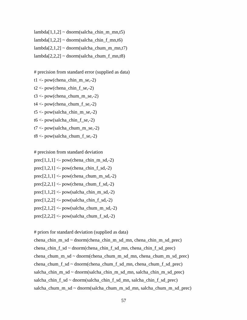
57
lambda[1,1,2] ~ dnorm(salcha_chin_m_mn,t5)
lambda[1,2,2] ~ dnorm(salcha_chin_f_mn,t6)
lambda[2,1,2] ~ dnorm(salcha_chum_m_mn,t7)
lambda[2,2,2] ~ dnorm(salcha_chum_f_mn,t8)
# precision from standard error (supplied as data)
t1 <- pow(chena_chin_m_se,-2)
t2 <- pow(chena_chin_f_se,-2)
t3 <- pow(chena_chum_m_se,-2)
t4 <- pow(chena_chum_f_se,-2)
t5 <- pow(salcha_chin_m_se,-2)
t6 <- pow(salcha_chin_f_se,-2)
t7 <- pow(salcha_chum_m_se,-2)
t8 <- pow(salcha_chum_f_se,-2)
# precision from standard deviation
prec[1,1,1] <- pow(chena_chin_m_sd,-2)
prec[1,2,1] <- pow(chena_chin_f_sd,-2)
prec[2,1,1] <- pow(chena_chum_m_sd,-2)
prec[2,2,1] <- pow(chena_chum_f_sd,-2)
prec[1,1,2] <- pow(salcha_chin_m_sd,-2)
prec[1,2,2] <- pow(salcha_chin_f_sd,-2)
prec[2,1,2] <- pow(salcha_chum_m_sd,-2)
prec[2,2,2] <- pow(salcha_chum_f_sd,-2)
# priors for standard deviation (supplied as data)
chena_chin_m_sd ~ dnorm(chena_chin_m_sd_mn, chena_chin_m_sd_prec)
chena_chin_f_sd ~ dnorm(chena_chin_f_sd_mn, chena_chin_f_sd_prec)
chena_chum_m_sd ~ dnorm(chena_chum_m_sd_mn, chena_chum_m_sd_prec)
chena_chum_f_sd ~ dnorm(chena_chum_f_sd_mn, chena_chum_f_sd_prec)
salcha_chin_m_sd ~ dnorm(salcha_chin_m_sd_mn, salcha_chin_m_sd_prec)
salcha_chin_f_sd ~ dnorm(salcha_chin_f_sd_mn, salcha_chin_f_sd_prec)
salcha_chum_m_sd ~ dnorm(salcha_chum_m_sd_mn, salcha_chum_m_sd_prec)

58
salcha_chum_f_sd ~ dnorm(salcha_chum_f_sd_mn, salcha_chum_f_sd_prec)
chena_chin_m_sd_prec <- pow(chena_chin_m_sd_sd,-2)
chena_chin_f_sd_prec <- pow(chena_chin_f_sd_sd,-2)
chena_chum_m_sd_prec <- pow(chena_chum_m_sd_sd,-2)
chena_chum_f_sd_prec <- pow(chena_chum_f_sd_sd,-2)
salcha_chin_m_sd_prec <- pow(salcha_chin_m_sd_sd,-2)
salcha_chin_f_sd_prec <- pow(salcha_chin_f_sd_sd,-2)
salcha_chum_m_sd_prec <- pow(salcha_chum_m_sd_sd,-2)
salcha_chum_f_sd_prec <- pow(salcha_chum_f_sd_sd,-2)
## parameters for run-timing logistic relationship
b0 <- mu.b0
b1 <- mu.b1
prec.b0 <- 1/0.6543603
prec.b1 <- 1/0.003060084
## priors for sex (supplied as data)
psex[1,1:2] ~ ddirch(alpha.sex.chin[])
psex[2,1:2] ~ ddirch(alpha.sex.chum[])
## posterior distributions of the totals for each species
N.chum <- sum(species[]) - n.fish
N.chin <- (2*n.fish) - sum(species[])
# some calculated subtotals - certain data regions needed to be expanded
Nchum_chena <- sum(species[1:9042]) - nchena
Nchin_chena <- (2*nchena) - sum(species[1:9042])
Nchum_salcha <- sum(species[9043:12361]) - nsalcha
Nchin_salcha <- (2*nsalcha) - sum(species[9043:12361])
for(k in 1:ndays) {
N.chum.day[k] <- sum(species[ifirst[k]:ilast[k]]) - nfishday[k]
N.chin.day[k] <- 2*nfishday[k] - sum(species[ifirst[k]:ilast[k]])

59
}
N.chum.before <- sum(species[9693:9704]) + sum(species[9712:9717]) - 18
N.chin.before <- 2*18 - sum(species[9693:9704]) - sum(species[9712:9717])
N.chum.after <- sum(species[9705:9711]) + sum(species[9718:9719]) - 9
N.chin.after <- 2*9 - sum(species[9705:9711]) - sum(species[9718:9719]) }

60

61
APPENDIX B:
JAGS CODE OF BAYESIAN HIERARCHICAL MODEL

62
Appendix B1.–JAGS code of Bayesian Hierarchical Model.
model {
for(j in 1:nyrs) {
for(i in 1:ndays){
y1[i,j] ~ dnorm(theta1[i,j], tausq1[j])
# y1[i,j] ~ dpois(theta1[i,j])
# Assume that run timing distribution takes log normal distribution
theta1[i,j] <- a1[j]*exp(-0.5*pow(log(x[i]/mu1[j])/b1[j],2))
# Assume that run timing distribution takes Extreme value distribution
# theta1[i,j] <- a1[j]*exp(-exp(-(x[i]-mu1[j])/b1[j])-(x[i]-mu1[j])/b1[j]+1)
# Assume that run timing distribution takes log-logistic distribution
# theta1[i,j] <- (a1[j]*(b1[j]/mu1[j])*pow((x[i]/mu1[j]),b1[j]-1))/pow(1+pow((x[i]/mu1[j]),b1[j]),2)
y2[i,j] ~ dnorm(theta2[i,j], tausq2[j])
# y2[i,j] ~ dpois(theta2[i,j])
# Assume that run timing distribution takes log normal distribution
theta2[i,j] <- a2[j]*exp(-0.5*pow(log(x[i]/mu2[j])/b2[j],2))
# Assume that run timing distribution takes Extreme value distribution
# theta2[i,j] <- a2[j]*exp(-exp(-(x[i]-mu2[j])/b2[j])-(x[i]-mu2[j])/b2[j]+1)
# Assume that run timing distribution takes log-logistic distribution
# theta2[i,j] <- (a2[j]*(b2[j]/mu2[j])*pow((x[i]/mu2[j]),b2[j]-1))/pow(1+pow((x[i]/mu2[j]),b2[j]),2)
}
}
# a[] indicates the maximum height (amplitude) of the function a>0
# mu[] indicates the function peaks when x = mu mu>0 : Peak timing
# b[] indicates peak width of the function b>0 standard deviation
# Priors
for(i in 1:nyrs) {
# Normal distribution Positive only
# a: is independent not hierarchical

63
a1[i] ~ dnorm(0,0.00001)T(0,)
b1[i] ~ dnorm(b01,b01.prec)T(0.16,)
mu1[i] <- mu2[i] + eps
a2[i] ~ dnorm(0,0.00001)T(0,)
b2[i] ~ dnorm(b02,b02.prec)T(0.16,)
mu2[i] ~ dnorm(mu02,mu02.prec)T(0,)
}
eps ~ dnorm(0,0.01)
prec.mu <- pow(sig.mu,-2)
sig.mu ~ dunif(0,2)
b01 ~ dnorm(0.5,0.001)T(0.16,)
mu01 ~ dnorm(25,0.001)T(0,)
b01.prec <-1/b01.ssq
b01.ssq <- b01.sigma*b01.sigma
b01.sigma ~ dunif(0,100)
mu01.prec <-1/mu01.ssq
mu01.ssq <- mu01.sigma*mu01.sigma
mu01.sigma ~ dunif(0,100)
b02 ~ dnorm(0.5,0.001)T(0.16,)
mu02 ~ dnorm(25,0.001)T(0,)
b02.prec <-1/b02.ssq
b02.ssq <- b02.sigma*b02.sigma
b02.sigma ~ dunif(0,100)
mu02.prec <-1/mu02.ssq
mu02.ssq <- mu02.sigma*mu02.sigma
mu02.sigma ~ dunif(0,100)
## This assumes that variance of each year is independent.
for(i in 1:nyrs) {
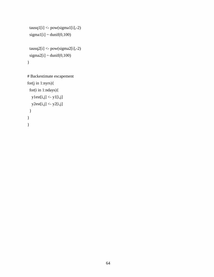
64
tausq1[i] <- pow(sigma1[i],-2)
sigma1[i] ~ dunif(0,100)
tausq2[i] <- pow(sigma2[i],-2)
sigma2[i] ~ dunif(0,100)
}
# Backestimate escapement
for(j in 1:nyrs){
for(i in 1:ndays){
y1est[i,j] <- y1[i,j]
y2est[i,j] <- y2[i,j]
}
}
}