Embed Size (px)
Citation preview
COST AND PROFIT EFFICIENCY IN EUROPEAN BANKS
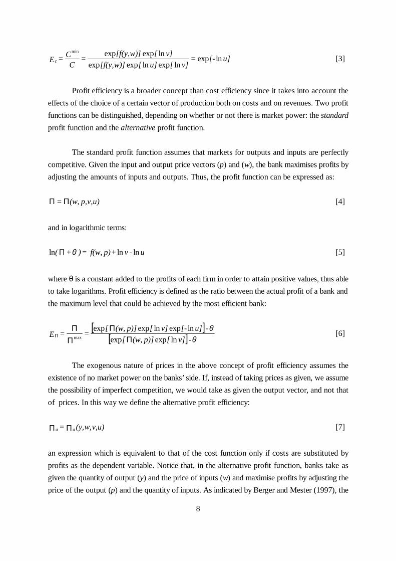
Joaquín Maudos, José Manuel Pastor, Francisco Pérez and Javier Quesada
WP-EC 99-12
Correspondence to: Joaquín Maudos.
IVIE
C/. Guardia Civil, 22, Esc. 2, 1º. 46020 Valencia (SPAIN)
Tel.: 34 963 930 816 / Fax:34 963 930 856 / e-mail: [email protected]
Editor: Instituto Valenciano de Investigaciones Económicas, S.A.
First Edition September 1999.
Depósito Legal: V-3182-1999
IVIE working-papers offer in advance the results of economic research under way in order to encourage a
discussion process before sending them to scientific journals for their final publication.
___________________
• The authors wish to thank David B. Humphrey for his comments and suggestions, and Juan Fernández de Guevarafor his help in preparing information. The paper is part of project SEC98-0895 of the CICYT.
2
COST AND PROFIT EFFICIENCY IN EUROPEAN BANKS
Joaquín Maudos, José M. Pastor, Francisco Pérez and Javier Quesada
ABSTRACT
The analysis of bank accounting ratios as indicators of competitiveness has beencomplemented and occasionally revised by the increasing use of more sophisticated indices ofefficiency. In recent years, over a hundred studies have analysed the efficiency of financialinstitutions, concentrating mostly on costs. However, the few available studies that estimate profitfrontier functions come up with efficiency levels that are much lower than cost efficiency levels,implying the existence of the most important inefficiencies on the revenue side. Also, few are thestudies that run comparisons at an international level, and none of these deals with profitefficiency. This paper analyses, by means of alternative techniques, both cost and profit efficiencyin a sample of 11 countries of the European Union for the period 1993-1996, again obtainingprofit efficiency levels lower than cost efficiency levels, as well as compatible results in thedifferent estimation procedures used.
Key words: Efficiency, European Banks
JEL: G21, G28
RESUMEN
El análisis de ratios contables como indicadores de competitividad ha sido completado yocasionalmente revisado por la creciente utilización de indicadores más sofisticados de eficiencia.En los últimos años, más de un centenar de trabajos han analizado la eficiencia de las institucionesfinancieras, centrándose mayoritariamente en la vertiente de los costes. Sin embargo, los escasosestudios que estiman funciones frontera de beneficios obtienen niveles de eficiencia en beneficiosmucho menores que en costes, lo que implica la existencia de importantes ineficiencias en lavertiente de los ingresos. Además, son pocos los estudios que realizan comparaciones a nivelinternacional, y ninguno de ellos analiza la eficiencia en beneficios. Por ese motivo, este trabajoanaliza la eficiencia en costes y beneficios en una muestra de 11 países de la Unión Europea enel periodo 1993-93 por medio de diversas técnicas frontera. Se obtienen niveles de eficiencia enbeneficios inferiores que en costes, siendo este resultado robusto a las distintas técnicas utilizadas.
Palabras clave: Eficiencia, banca europea.
3
1. Introduction
For many years, the comparison of bank accounting ratios as well as banking sectors has
shown the existence of remarkable differences in average costs. Also, wide ranges of ROA and
ROE have been found, although these results are more difficult to evaluate due to their greater
instability. Both types of evidence have supported the view that differences in the efficiency of
banks are due to the existence of a low level of competitiveness. This view has been reconsidered
as the liberalisation process brought about a clear intensification of competition. However, the
dispersion of costs and profits continues to be notable among companies and among countries,
which calls into question the suitability of accounting indicators in portraying the productive
efficiency achieved.
On the cost side, the analysis of the differences in average costs has been oriented for
many years towards the question of economies of scale and, to a lesser extent, to the study of
scope economies (specialisation).
In recent years, the tendency has changed towards the analysis of the X-efficiency of
banks, giving rise to a large number of studies. The existence for a group of banks of similar size
of a greater dispersion of average costs than that for banks of different sizes has made X-
efficiency a much more important potential source of cost reduction than the achievement of an
optimum size of production for minimising average costs. Thus, the efficiency analysis has
currently replaced economies of scale as the main objective of empirical research.
Many X-efficiency studies consider different output vectors, and so they are limited by the
available information. Thus, they consider the impact of specialisation on costs, and this is one
reason why X-inefficiencies do not generally present such a wide range as accounting ratios do.
However, the objective of maximising profits does not only require that goods and
services be produced at the minimum cost. It also demands the maximum volume of revenues. In
this sense, computing profit efficiency constitutes a more important source of information for
bank management than the partial vision offered by the analysis of cost efficiency.
The scarce available evidence has shown greater profit inefficiency than cost inefficiency
levels. This result could be an indication of the important inefficiencies on the revenue side, either
due to the choice of the wrong composition of output, or to the establishment of an erroneous
pricing policy.
4
Of the 130 studies reviewed in the extensive survey carried out by Berger and Humphrey
(1997) on efficiency in financial institutions, only 9 studies analysed efficiency in profits1. With the
exception of the study by Miller and Noulas (1996), profit efficiency is found lower than cost
efficiency, the former reaching an average value of 64% for the studies referring to the U.S.
banking system. However, in only three of the studies (Berger and Mester, 1997; Lozano, 1997
and Rogers, 1998) are the results compared using a single sample, with profit inefficiency always
shown to be the largest one2.
Berger et al. (1993) is the first study that compares profit with cost efficiency. This paper
breaks down profit inefficiency into two parts, one part attributable to technical causes and the
other one associated with problems of allocation. The study finds inefficiency levels of 50%, most
of them of the technical type. According to this result, inefficiency is explained better by an
insufficient level of income than by an excess of costs. This outcome suggests that estimates based
only on cost underestimate total inefficiency.
As in Berger et al. (1993), the studies by Akhavein et al. (1994), DeYoung and Nolle
(1995) and Rogers (1998), referring to the U.S. banking sector found that the major part of
inefficiency was due to insufficient income rather than to excessive costs. In a recent study by
Berger and Mester (1997), the greater importance of profit inefficiency is shown. Using a panel
of nearly 6,000 U.S. banks for each year (from 1990 to 1995) Berger and Mester estimate their
preferred model, a Fourier-flexible specification estimated by the distribution free approach DFA
method. They find a value of 46.3% for the alternative profit efficiency and of 54.9% for the
standard profit efficiency3, in contrast to an average cost efficiency of 87%. Also, the standard
deviation of profit inefficiency is nearly four times higher than that of cost inefficiency, which is
indicative of the greater dispersion of the first type of inefficiencies.
Another interesting result of Berger and Mester’s study is that, contrary to what could
have initially been expected, profit efficiency is not positively correlated with cost efficiency4,
suggesting the possibility that cost and revenue inefficiencies may be negatively correlated. This
1 Two further papers should be added to their list, namely, Rogers (1998) and De Young and Hasan (1998).2 In Berger and Mester (1997) profit efficiency is approximately half of cost efficiency. In the case of theSpanish savings banks, using the thick frontier approach, Lozano (1997) obtains a profit efficiency levelmore than twice the size of that of cost efficiency. Finally, Rogers (1998) obtains an average profit efficiencyof 69.2% and a cost efficiency of 75,6%, with a lower revenue efficiency of 43,7%. 3 Berger and Mester (1997) define alternative profit efficiency as when banks have market power to set pricesand standard profit efficiency as when they behave as price takers.4 This result is also achieved in Rogers (1998), although with a positive correlation between income and profitefficiency.
5
result indicates that a bank with higher costs may compensate this apparent inefficiency by
achieving higher revenues than its competitors, either using a different composition of its vector
of production or by benefiting from a greater market power in price setting derived from its
specialisation. Thus, part of what we measure as cost inefficiency may be contaminated by the
output composition, making possible that an output vector of more quality could be more costly
but not necessarily inefficient. Alternatively, the estimation of a frontier profit function could
capture productive specialisation, allowing the higher revenues received by banks that produce
differentiated or higher quality outputs to compensate for the higher costs incurred.
Another issue insufficiently dealt with in the extensive literature on bank efficiency refers
to international comparisons. The four studies reviewed by Berger and Humphrey (1997)5 find
substantial differences of cost efficiency by countries, although none of them considers profit
efficiency. As they are centered exclusively on the cost side, the results must be interpreted with
caution. In fact, many factors can influence cost efficiency, like the different regulatory
environments, the intensity of competition, the output specialisation, the input quality, etc.
Consequently, the estimation of the alternative profit efficiency, which takes into account the
different degree of competition as well as the effect of output quality on revenues, seems to be a
more appropriate way of running international comparisons.
To sum up, there are two areas in which the available evidence on bank efficiency is very
limited: a) estimation of profit efficiency and its comparison with cost efficiency; and b)
international efficiency comparisons. The intersection of the two areas is an empty set. This is the
domain in which this study is situated; the analysis of cost and profit efficiency in a sample of 11
countries, full members of the European Union during the period 1993-1996.
The establishment of a common currency area in most of the countries in the sample will
strongly reinforce the mobility of financial flows, as well as cross-border banking activities.
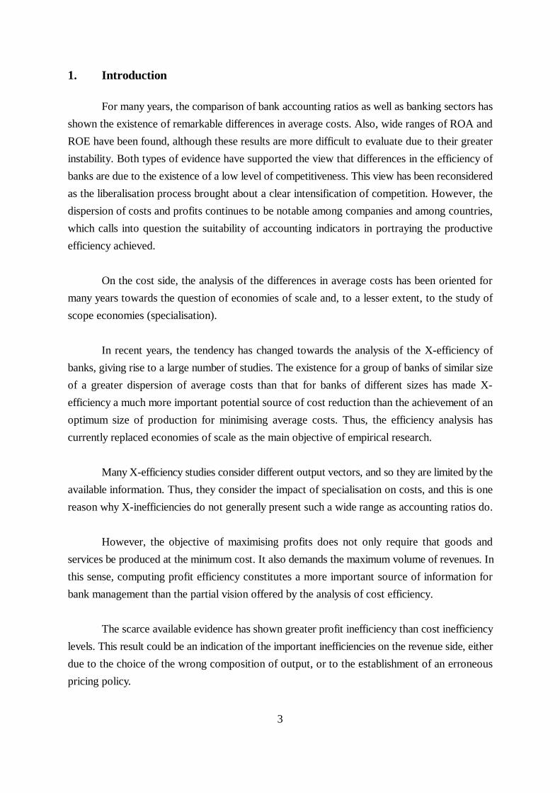
However, the current differences of cost and the wide variations of profitability among different
banking systems (see figures 1 and 2) continue to raise questions about the future consequences
of the gradual integration of banks in an effectively integrated European banking system. Thus,
5 Fecher and Pestiau (1993), Pastor et al. (1997), Ruthenberg and Elias (1996) and Allen and Rai (1996).
6
GermanyAustria
HollandUnited Kingdom
DenmarkLuxembourg
FranceFinland
PortugalItaly
SpainSweden
BelgiumGreece
0
2
4
6
8
10
12
Financial CostsOperating Costs
Note: Ireland is not incuded in the "Bank Profitability" data base.Source: Bank Profitability (OECD).
Figure 1. Average costs in the European banking systems. 1995(% Total assets)
FinlandFrance
BelgiumItaly
AustriaLuxembourg
GermanyPortugal
HollandSpain
United KingdomGreece
SwedenDenmark
-0,5
0
0,5
1
1,5
RO
A
ROAROE
Figure 2. Profitability in the European banking systems. 1995
7
the study of the different efficiencies among countries of the European Union will explain the
competitive starting position of each country, which may condition its capacity to respond to the
new scenario.
With this objective, the paper is structured as follows: Section 2 describes the concepts
of cost and profit efficiency, specifying the frontier functions to be estimated; Section 3 comments
briefly on the different approaches used for the estimation of efficiency and examines how the
technique chosen influences the results; In section 4 the sample data are described and empirical
results obtained; Section 5 draws conclusions.
2. Cost efficiency vs. profit efficiency
Cost and profit efficiency definitions correspond, respectively, to two important economic
objectives: cost minimisation and profit maximisation. Cost efficiency is the ratio between the
minimum cost at which it is possible to attain a given volume of production and the cost actually
incurred. Thus, an efficiency value of Ec implies that it would be possible to produce the same
vector of production, saving (1-Ec)·100 per cent of the costs. Efficiency ranges over the (0,1]
interval, and equals one for the best-practice bank in the sample.
The costs of a bank depend on the output vector (y), the price of inputs (w), the level of
cost inefficiency (u) and a set of random factors (v) which incorporate the effect of errors in the
measurement of variables, bad luck, etc. Thus, the cost function is expressed as:
v)u,w,C(y,=C [1]
or in logarithmic terms, and assuming that the efficiency and random error terms are
multiplicatively separable from the remaining arguments of the cost function,
v+u+w)f(y,=C lnlnln [2]
On the basis of the estimation of a particular functional form f, cost efficiency (Ec) is
measured as the ratio between the minimum costs (Cmin) necessary to produce the output vector
and the costs actually incurred (C):
8
u][-=v][u][w)][f(y,
v][w)][f(y,=
CC=Ec lnexp
lnexplnexpexp
lnexpexpmin
[3]
Profit efficiency is a broader concept than cost efficiency since it takes into account the
effects of the choice of a certain vector of production both on costs and on revenues. Two profit
functions can be distinguished, depending on whether or not there is market power: the standard
profit function and the alternative profit function.
The standard profit function assumes that markets for outputs and inputs are perfectly
competitive. Given the input and output price vectors (p) and (w), the bank maximises profits by
adjusting the amounts of inputs and outputs. Thus, the profit function can be expressed as:
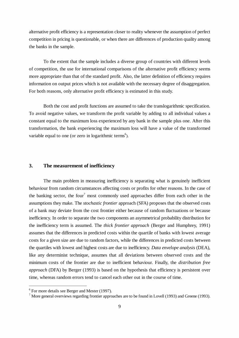
u)v,p,(w,= ΠΠ [4]
and in logarithmic terms:
u-v+p)f(w,=)+( lnlnln θΠ [5]
where θ is a constant added to the profits of each firm in order to attain positive values, thus able
to take logarithms. Profit efficiency is defined as the ratio between the actual profit of a bank and
the maximum level that could be achieved by the most efficient bank:
[ ][ ] θ
θ-v][p)](w,[
-u][-v][p)](w,[==E
lnexpexp
lnexplnexpexpmax Π
ΠΠ
ΠΠ [6]
The exogenous nature of prices in the above concept of profit efficiency assumes the
existence of no market power on the banks’ side. If, instead of taking prices as given, we assume
the possibility of imperfect competition, we would take as given the output vector, and not that
of prices. In this way we define the alternative profit efficiency:
u)v,w,(y,= aa ΠΠ [7]
an expression which is equivalent to that of the cost function only if costs are substituted by
profits as the dependent variable. Notice that, in the alternative profit function, banks take as
given the quantity of output (y) and the price of inputs (w) and maximise profits by adjusting the
price of the output (p) and the quantity of inputs. As indicated by Berger and Mester (1997), the
9
alternative profit efficiency is a representation closer to reality whenever the assumption of perfect
competition in pricing is questionable, or when there are differences of production quality among
the banks in the sample.
To the extent that the sample includes a diverse group of countries with different levels
of competition, the use for international comparisons of the alternative profit efficiency seems
more appropriate than that of the standard profit. Also, the latter definition of efficiency requires
information on output prices which is not available with the necessary degree of disaggregation.
For both reasons, only alternative profit efficiency is estimated in this study.
Both the cost and profit functions are assumed to take the translogarithmic specification.
To avoid negative values, we transform the profit variable by adding to all individual values a
constant equal to the maximum loss experienced by any bank in the sample plus one. After this
transformation, the bank experiencing the maximum loss will have a value of the transformed
variable equal to one (or zero in logarithmic terms6).
3. The measurement of inefficiency
The main problem in measuring inefficiency is separating what is genuinely inefficient
behaviour from random circumstances affecting costs or profits for other reasons. In the case of
the banking sector, the four7 most commonly used approaches differ from each other in the
assumptions they make. The stochastic frontier approach (SFA) proposes that the observed costs
of a bank may deviate from the cost frontier either because of random fluctuations or because
inefficiency. In order to separate the two components an asymmetrical probability distribution for
the inefficiency term is assumed. The thick frontier approach (Berger and Humphrey, 1991)
assumes that the differences in predicted costs within the quartile of banks with lowest average
costs for a given size are due to random factors, while the differences in predicted costs between
the quartiles with lowest and highest costs are due to inefficiency. Data envelope analysis (DEA),
like any determinist technique, assumes that all deviations between observed costs and the
minimum costs of the frontier are due to inefficient behaviour. Finally, the distribution free
approach (DFA) by Berger (1993) is based on the hypothesis that efficiency is persistent over
time, whereas random errors tend to cancel each other out in the course of time.
6 For more details see Berger and Mester (1997).7 More general overviews regarding frontier approaches are to be found in Lovell (1993) and Greene (1993).
10
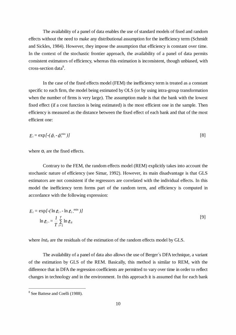
The availability of a panel of data enables the use of standard models of fixed and random
effects without the need to make any distributional assumption for the inefficiency term (Schmidt
and Sickles, 1984). However, they impose the assumption that efficiency is constant over time.
In the context of the stochastic frontier approach, the availability of a panel of data permits
consistent estimators of efficiency, whereas this estimation is inconsistent, though unbiased, with
cross-section data8.
In the case of the fixed effects model (FEM) the inefficiency term is treated as a constant
specific to each firm, the model being estimated by OLS (or by using intra-group transformation
when the number of firms is very large). The assumption made is that the bank with the lowest
fixed effect (if a cost function is being estimated) is the most efficient one in the sample. Then
efficiency is measured as the distance between the fixed effect of each bank and that of the most
efficient one:
)]-[-(=E iii αα ˆˆexp min [8]
where αi are the fixed effects.
Contrary to the FEM, the random effects model (REM) explicitly takes into account the
stochastic nature of efficiency (see Simar, 1992). However, its main disadvantage is that GLS
estimators are not consistent if the regressors are correlated with the individual effects. In this
model the inefficiency term forms part of the random term, and efficiency is computed in
accordance with the following expression:
εε
εε
ˆlnˆln
ˆlnˆlnexp min
it
T
1=ti
iii
T
1=.
)].-.[-(=E
∑[9]
where lnεit are the residuals of the estimation of the random effects model by GLS.
The availability of a panel of data also allows the use of Berger´s DFA technique, a variant
of the estimation by GLS of the REM. Basically, this method is similar to REM, with the
difference that in DFA the regression coefficients are permitted to vary over time in order to reflect
changes in technology and in the environment. In this approach it is assumed that for each bank
8 See Battese and Coelli (1988).
11
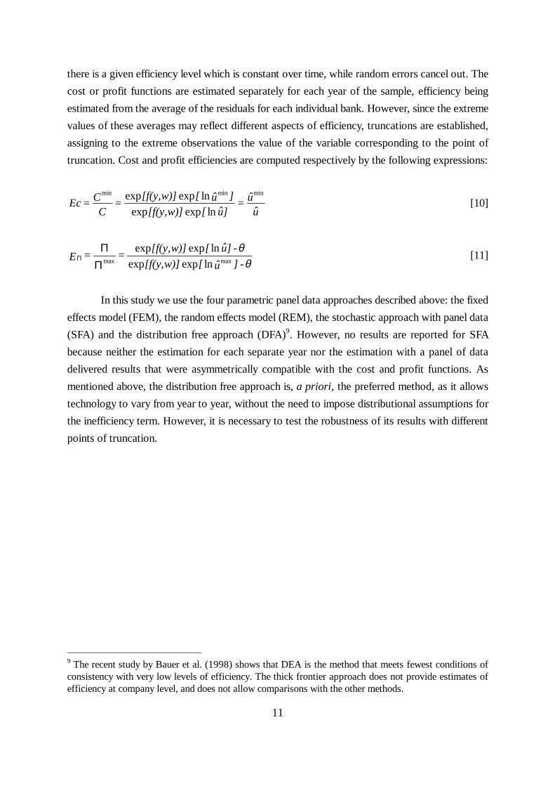
there is a given efficiency level which is constant over time, while random errors cancel out. The
cost or profit functions are estimated separately for each year of the sample, efficiency being
estimated from the average of the residuals for each individual bank. However, since the extreme
values of these averages may reflect different aspects of efficiency, truncations are established,
assigning to the extreme observations the value of the variable corresponding to the point of
truncation. Cost and profit efficiencies are computed respectively by the following expressions:
uu=
]u[w)][f(y,
]u[w)][f(y,=
CC=Ec
ˆˆ
ˆlnexpexpˆlnexpexp minminmin
[10]
θθ-]u[w)][f(y,
-]u[w)][f(y,==E
ˆlnexpexp
ˆlnexpexpmaxmaxΠ
ΠΠ [11]
In this study we use the four parametric panel data approaches described above: the fixed
effects model (FEM), the random effects model (REM), the stochastic approach with panel data
(SFA) and the distribution free approach (DFA)9. However, no results are reported for SFA
because neither the estimation for each separate year nor the estimation with a panel of data
delivered results that were asymmetrically compatible with the cost and profit functions. As
mentioned above, the distribution free approach is, a priori, the preferred method, as it allows
technology to vary from year to year, without the need to impose distributional assumptions for
the inefficiency term. However, it is necessary to test the robustness of its results with different
points of truncation.
9 The recent study by Bauer et al. (1998) shows that DEA is the method that meets fewest conditions ofconsistency with very low levels of efficiency. The thick frontier approach does not provide estimates ofefficiency at company level, and does not allow comparisons with the other methods.
12
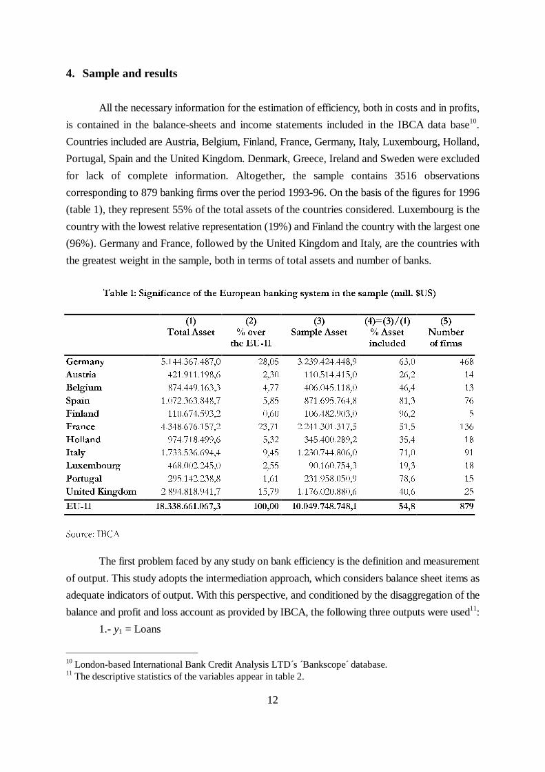
4. Sample and results
All the necessary information for the estimation of efficiency, both in costs and in profits,
is contained in the balance-sheets and income statements included in the IBCA data base10.
Countries included are Austria, Belgium, Finland, France, Germany, Italy, Luxembourg, Holland,
Portugal, Spain and the United Kingdom. Denmark, Greece, Ireland and Sweden were excluded
for lack of complete information. Altogether, the sample contains 3516 observations
corresponding to 879 banking firms over the period 1993-96. On the basis of the figures for 1996
(table 1), they represent 55% of the total assets of the countries considered. Luxembourg is the
country with the lowest relative representation (19%) and Finland the country with the largest one
(96%). Germany and France, followed by the United Kingdom and Italy, are the countries with
the greatest weight in the sample, both in terms of total assets and number of banks.
7DEOH �� 6LJQLILFDQFH RI WKH (XURSHDQ EDQNLQJ V\VWHP LQ WKH VDPSOH �PLOO� �86�
���7RWDO $VVHW
���� RYHU
WKH (8���
���6DPSOH $VVHW
��� �������� $VVHWLQFOXGHG
���1XPEHURI ILUPV
*HUPDQ\ ��������������� ����� ��������������� ���� ���
$XVWULD ������������� ���� ������������� ���� ��
%HOJLXP ������������� ���� ������������� ���� ��
6SDLQ ��������������� ���� ������������� ���� ��
)LQODQG ������������� ���� ������������� ���� �
)UDQFH ��������������� ����� ��������������� ���� ���
+ROODQG ������������� ���� ������������� ���� ��
,WDO\ ��������������� ���� ��������������� ���� ��
/X[HPERXUJ ������������� ���� ������������ ���� ��
3RUWXJDO ������������� ���� ������������� ���� ��
8QLWHG .LQJGRP ��������������� ����� ��������������� ���� ��
(8��� ���������������� ������ ���������������� ���� ���
6RXUFH� ,%&$
The first problem faced by any study on bank efficiency is the definition and measurement
of output. This study adopts the intermediation approach, which considers balance sheet items as
adequate indicators of output. With this perspective, and conditioned by the disaggregation of the
balance and profit and loss account as provided by IBCA, the following three outputs were used11:
1.- y1 = Loans
10 London-based International Bank Credit Analysis LTD´s ´Bankscope database.11 The descriptive statistics of the variables appear in table 2.
13
2.- y2 = Other earning assets
3.- y3 = Deposits
7DEOH �� 'HVFULSWLYH VWDWLVWLFV RI WKH YDULDEOHV� �������
$YHUDJH 6WG� &RHI� 9DU�
7& WRWDO FRVWV �ILQDQFLDO � RSHUDWLQJ� ��������� ��������� �����
3 RSHUDWLQJ SURILW �QHW LQFRPH � SURYLVLRQV� ������� ������� �����
$ WRWDO DVVHWV ���������� ����������� �����
\� ORDQV ���������� ���������� �����
\� RWKHU HDUQLQJ DVVHVWV ���������� ���������� �����
\� ORDQDEOH IXQGV ���������� ���������� 3,051Z� SULFH RI ORDQDEOH IXQGV ����� ����� �����
Z� SULFH RI ODERU ����� ����� �����
Z� SULFH RI SK\VLFDO FDSLWDO ����� ������ �����
7&�$ ����� ����� �����
3�$ ����� ����� �����
1RWH� 7&� 3� $� \�� \� LQ PLOO� RI �86�
6RXUFH� ,%&$
The second type of variables appearing in the cost and profit function are the prices of
productive factors. Three inputs were selected and, consequently, the following input prices were
used:
1.- w1= Cost of loanable funds, computed by dividing financial costs by their
corresponding liabilities.
2.- w2= Cost of labor. Since IBCA does not provide information on the number of
employees for each bank, the price of labor has been calculated by dividing personnel costs by
total assets12.
3.- w3= Cost of physical capital, defined as the ratio between expenditures on plant and
equipment and the book value of physical capital.
12 This approximation is common in all studies using IBCA data. The variable used can be interpreted as laborcost per worker adjusted for differences in labor productivity, since (PE/A)=(PE/L)(L/A) where PE=personnel expenses, A=total assets and L=labor.
14
The translog frontier cost function finally estimated is as follows:
u+v+/a)y()w/w(+/a)y(/a)y(2
1+/a)y(
+)w/w()w/w(2
1+)w/w(+=a)w(C/
n3i
3
1=n
3
1=imnnm
3
1=m
3
1=nnn
3
1=i
3j3iij
3
1=j
3
1=i3ii
3
1=i3
lnlnlnlnlnlnln
lnlnlnln
ργγ
ββα
∈∑∑∑∑∑
∑∑∑
[12]
where the restrictions of symmetry and linear homogeneity have been imposed on input prices.
Notice, furthermore, that costs and outputs are expressed as the ratio to average total assets (a)13.
In the estimation of the cost function both financial and operating costs are included. In
the case of the profit function, the variable to be explained is the operating profit14.
In the alternative profit function the dependent variable is ln[(Π/w3a) + |(Π/w3a)min| + 1],
where we add the minimum value of profits plus one in order to ensure a positive value for the
transformed variable. These transformations are considered later when the values of efficiency
for each country are estimated15.
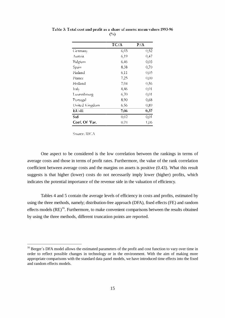
Table 3 shows average costs per unit of assets and the return on assets of the banking
systems considered as an average for the period (1993-96). The coefficients of variation show
greater dispersion for profit efficiency than for cost efficiency. Thus, sectors with ROA’s over
0.7% (Spain and the U.K.) coexist with sectors with profit rates close to zero (Italy, France and
Luxembourg).
13 The profit variable is also expressed as ratio to total assets in the translog frontier function. As indicatedby Berger and Mester, there are three reasons for proceeding in this way: 1) it reduces possible problems ofheteroskedasticity; 2) it reduces possible biases of scale; 3) the dependent variable used in the estimation ofthe frontier profit function is an indicator of profitability over assets (ROA), and therefore has a cleareconomic interpretation. Berger and Mester (1997) use equity instead of assets as the variable ofnormalisation. In this study the preferred scale variable was total assets, since institutional differences amongdifferent types of banks (savings banks vs. commercial banks) could affect the definition of equity.14 The variable of profits used is what the IBCA calls operating profit, which is the net income minusprovisions (provisions for loan losses and other provisions).15 As in Berger and Mester (1997), although not required, we assume linear homogeneity in prices in theprofit function, to keep it equivalent to the estimated cost function.
15
7DEOH �� 7RWDO FRVW DQG SURILW DV D VKDUH RI DVVHWV� PHDQ YDOXHV ����������
7&�$ 3�$
*HUPDQ\ ���� ����
$XVWULD ���� ����
%DOJLXP ���� ����
6SDLQ ���� ����
)LQODQG ���� ����
)UDQFH ���� ����
+ROODQG ���� ����
,WDO\ ���� �����
/X[HPERXUJ ���� ����
3RUWXJDO ���� ����
8QLWHG .LQJGRP ���� ����
(8��� ���� ����
6WG ���� ����
&RHI� 2I 9DU� ���� ����
6RXUFH� ,%&$
One aspect to be considered is the low correlation between the rankings in terms of
average costs and those in terms of profit rates. Furthermore, the value of the rank correlation
coefficient between average costs and the margins on assets is positive (0.43). What this result
suggests is that higher (lower) costs do not necessarily imply lower (higher) profits, which
indicates the potential importance of the revenue side in the valuation of efficiency.
Tables 4 and 5 contain the average levels of efficiency in costs and profits, estimated by
using the three methods, namely; distribution-free approach (DFA), fixed effects (FE) and random
effects models (RE)16. Furthermore, to make convenient comparisons between the results obtained
by using the three methods, different truncation points are reported.
16 Berger´s DFA model allows the estimated parameters of the profit and cost function to vary over time inorder to reflect possible changes in technology or in the environment. With the aim of making moreappropriate comparisons with the standard data panel models, we have introduced time effects into the fixedand random effects models.
16
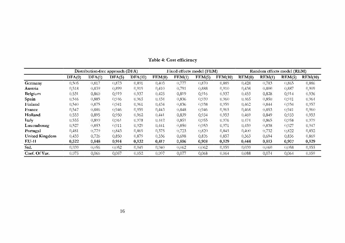
7DEOH �� &RVW HIILFLHQF\
'LVWULEXWLRQ�IUHH DSSURDFK �')$� )L[HG HIIHFWVPRGHO �)(0� 5DQGRP HIIHFWV PRGHO �5(0�
')$��� ')$��� ')$��� ')$���� )(0��� )(0��� )(0��� )(0���� 5(0��� 5(0��� 5(0��� 5(0����
*HUPDQ\ ����� ����� ����� ����� ����� ����� ����� ����� ����� ����� ����� �����
$XVWULD ����� ����� ����� ����� ����� ����� ����� ����� ����� ����� ����� �����
%HOJLXP ����� ����� ����� ����� ����� ����� ����� ����� ����� ����� ����� �����
6SDLQ ����� ����� ����� ����� ����� ����� ����� ����� ����� ����� ����� �����
)LQODQG ����� ����� ����� ����� ����� ����� ����� ����� ����� ����� ����� �����
)UDQFH ����� ����� ����� ����� ����� ����� ����� ����� ����� ����� ����� �����
+ROODQG ����� ����� ����� ����� ����� ����� ����� ����� ����� ����� ����� �����
,WDO\ ����� ����� ����� ����� ����� ����� ����� ����� ����� ����� ����� �����
/X[HPERXUJ ����� ����� ����� ����� ����� ����� ����� ����� ����� ����� ����� �����
3RUWXJDO ����� ����� ����� ����� ����� ����� ����� ����� ����� ����� ����� �����
8QLWHG .LQJGRP ����� ����� ����� ����� ����� ����� ����� ����� ����� ����� ����� �����
(8��� ����� ����� ����� ����� ����� ����� ����� ����� ����� ����� ����� �����
6WG� ����� ����� ����� ����� ����� ����� ����� ����� ����� ����� ����� �����
&RHI� 2I 9DU� ����� ����� ����� ����� ����� ����� ����� ����� ����� ����� ����� �����
17
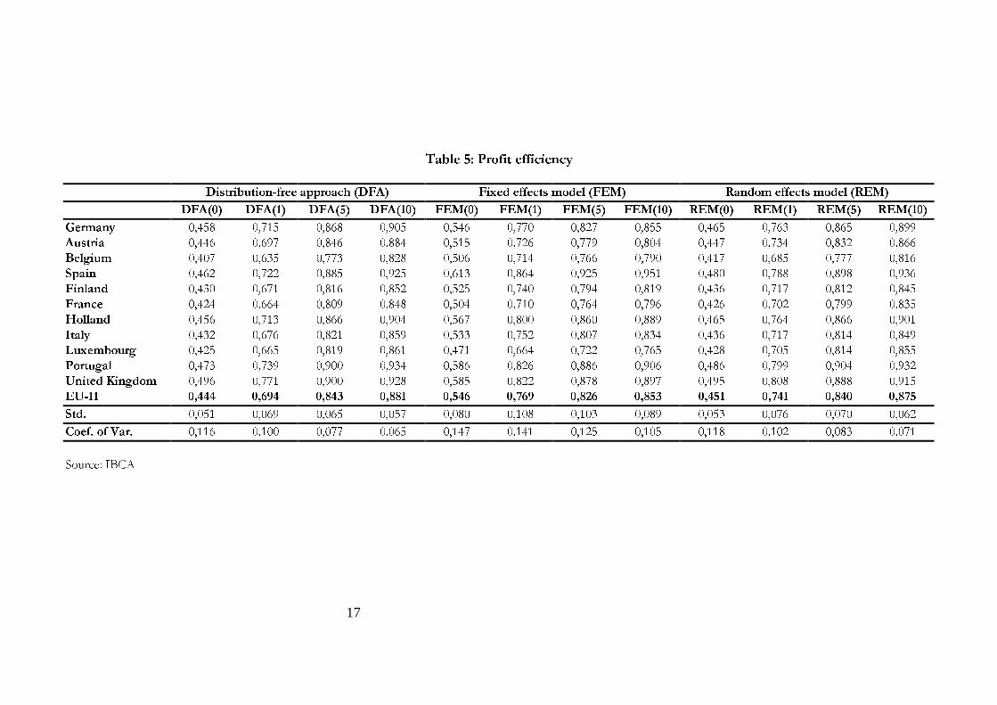
7DEOH �� 3URILW HIILFLHQF\
'LVWULEXWLRQ�IUHH DSSURDFK �')$� )L[HG HIIHFWVPRGHO �)(0� 5DQGRP HIIHFWV PRGHO �5(0�
')$��� ')$��� ')$��� ')$���� )(0��� )(0��� )(0��� )(0���� 5(0��� 5(0��� 5(0��� 5(0����
*HUPDQ\ ����� ����� ����� ����� ����� ����� ����� ����� ����� ����� ����� �����
$XVWULD ����� ����� ����� ����� ����� ����� ����� ����� ����� ����� ����� �����
%HOJLXP ����� ����� ����� ����� ����� ����� ����� ����� ����� ����� ����� �����
6SDLQ ����� ����� ����� ����� ����� ����� ����� ����� ����� ����� ����� �����
)LQODQG ����� ����� ����� ����� ����� ����� ����� ����� ����� ����� ����� �����
)UDQFH ����� ����� ����� ����� ����� ����� ����� ����� ����� ����� ����� �����
+ROODQG ����� ����� ����� ����� ����� ����� ����� ����� ����� ����� ����� �����
,WDO\ ����� ����� ����� ����� ����� ����� ����� ����� ����� ����� ����� �����
/X[HPERXUJ ����� ����� ����� ����� ����� ����� ����� ����� ����� ����� ����� �����
3RUWXJDO ����� ����� ����� ����� ����� ����� ����� ����� ����� ����� ����� �����
8QLWHG .LQJGRP ����� ����� ����� ����� ����� ����� ����� ����� ����� ����� ����� �����
(8��� ����� ����� ����� ����� ����� ����� ����� ����� ����� ����� ����� �����
6WG� ����� ����� ����� ����� ����� ����� ����� ����� ����� ����� ����� �����
&RHI� RI 9DU� ����� ����� ����� ����� ����� ����� ����� ����� ����� ����� ����� �����
6RXUFH� ,%&$
18
The levels of cost efficiency depend greatly on the truncation point chosen. Thus, for
example, in DFA the cost efficiency of the average of the countries considered changes from
52.2% to 84.8% when only 1% of the extreme values are replaced by the value of the truncation
point. The efficiency increases up to 91.4% when using 5% truncation, but the increase tapers off
after this point. What this result suggests is that even after using averages for several years, there
is still a high relative weight of random factors, other than inefficiency, that do not cancel each
other out in the course of time. This effect has to be alleviated by substituting the more extreme
values with those of the points of truncation for a correct valuation and quantification of
inefficiency levels. The fact that the change from 5% to 10% truncation does not substantially
alter the levels of efficiency leads us to consider 5% a reasonable level of truncation for valuing
the results17.
The results at 5% truncation show a level of cost efficiency of 91.4% for the average of
the 11 countries of the European Union considered. According to this estimate it would be
possible to reduce costs by about 8%-9%, simply by eliminating X-inefficiencies. Looking at
particular countries we find Portugal and the United Kingdom to be the least efficient countries,
with values near 15% of total costs, and Italy standing at the opposite extreme with an inefficiency
level of 4%.
The levels of efficiency estimated, and the dispersion of the values, are fairly similar in the
FE and RE models. Thus, again taking as reference a truncation of 5%, the average efficiency of
the FE model is 90.8%, very similar to the 90.7% of the RE model. The identification of the most
and least efficient banking sectors is independent of the frontier function used. In both FE and RE
models, Italy and Portugal are, respectively, the most efficient and inefficient countries. Thus, both
in terms of average values and in identifying the most and least efficient banking sectors, the
results are robust to the technique used for estimation. These results are conditions of consistency
sine qua non for ensuring the credibility and utility of indicators of efficiency18.
The results corresponding to alternative profit efficiency appear in table 5. Once more, the
levels of efficiency vary considerably depending on the point of truncation chosen. Again, the
change from 5% to 10% causes quite a small change in magnitude, so we will centre on the results
corresponding to 5%.
17 This result corresponds with that obtained in Berger and Mester (1997) and Berger (1993).18 See Bauer et al. (1998) for a full description of conditions of consistency.

19
The first result to note is the existence of lower levels of profit efficiency than of cost
efficiency. These results are similar to those obtained in other studies (Berger and Mester (1997)
and Rogers (1998) for the US banking system, and Lozano (1997) for the Spanish savings banks).
Thus, and once again independently of the method used, profit efficiency is in the neighbourhood
of around 82%-84%, 7-8 percentage points lower than the cost efficiency level19.
The information by countries shows a range of variation relatively similar to that obtained
before in terms of cost efficiency. Thus, the difference between the least efficient sector (Belgium)
and the most efficient (Portugal and the United Kingdom) is 12 percentage points. Except for
Portugal and the United Kingdom, the profit efficiency of each country is always lower than cost
efficiency, the extreme cases being the difference of about 12-14 percentage points in Belgium,
Finland, France and Italy. On the other hand, in Germany the difference between cost efficiency
and profit efficiency is only about 1 percentage point.
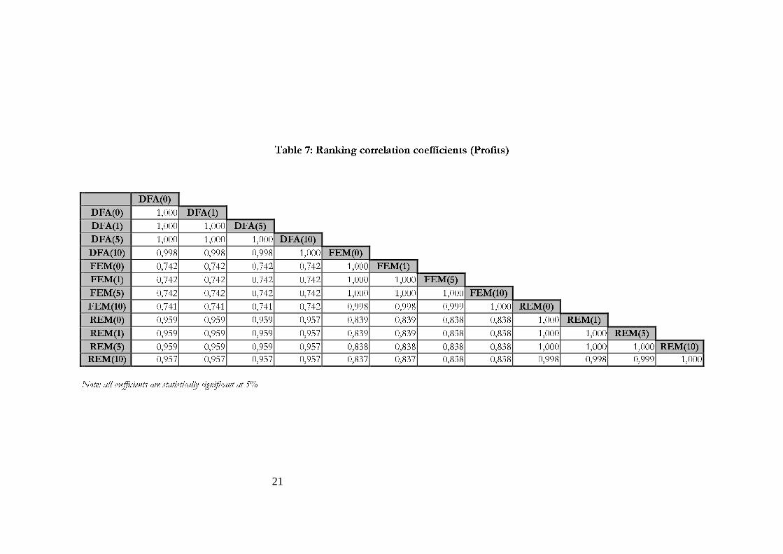
To test for the consistency of the rankings of efficiency, tables 6 and 7 contain the values
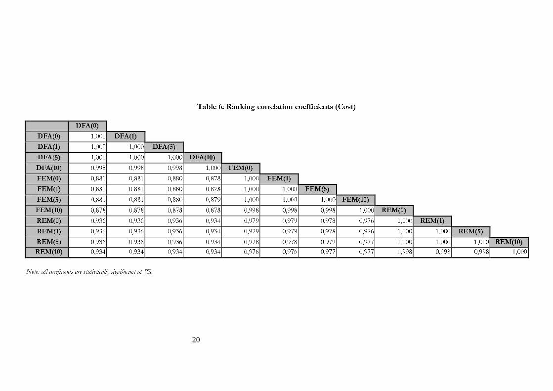
of the rank correlation coefficients. Two results can be highlighted:
1.- For the same frontier technique, the ranking in efficiency is very similar independently
of the level of truncation chosen, the value of the coefficient being 0.98-0.99 in all cases.
2.- The coefficients of correlation between efficiency rankings using different techniques
are very high and statistically significant. A high correlation is also observed between the
REM and DFA methods, a logical result if it is taken into account that in both methods
inefficiency is estimated from the residues of the regression20. The lowest values of the
coefficients of correlation are observed in the case of the FE model, although the
magnitude of the coefficient is high in all cases.
19 The higher volatility of ROA as compared to that of average costs could explain the lower profit efficiencylevel with respect to the cost efficiency level. To test for this possibility, the cost and profit functions were re-estimated using average values as opposed to annual observations. Very similar results were obtained byapplying corrected minimum squares with different points of truncation.20 In both models the stochastic nature of the inefficiency term is taken into account, while in the fixed effectsmodel inefficiency has a determinist character (see Simar, 19).
20
7DEOH �� 5DQNLQJ FRUUHODWLRQ FRHIILFLHQWV �&RVW�
')$���
')$��� ����� ')$���
')$��� ����� ����� ')$���
')$��� ����� ����� ����� ')$����
')$���� ����� ����� ����� ����� )(0���
)(0��� ����� ����� ����� ����� ����� )(0���
)(0��� ����� ����� ����� ����� ����� ����� )(0���
)(0��� ����� ����� ����� ����� ����� ����� ����� )(0����
)(0���� ����� ����� ����� ����� ����� ����� ����� ����� 5(0���
5(0��� ����� ����� ����� ����� ����� ����� ����� ����� ����� 5(0���
5(0��� ����� ����� ����� ����� ����� ����� ����� ����� ����� ����� 5(0���
5(0��� ����� ����� ����� ����� ����� ����� ����� ����� ����� ����� ����� 5(0����
5(0���� ����� ����� ����� ����� ����� ����� ����� ����� ����� ����� ����� �����
1RWH� DOO FRHHILFLHQWV DUH VWDWLVWLFDOO\ VLJQLIXFDQW DW ��
21
7DEOH �� 5DQNLQJ FRUUHODWLRQ FRHIILFLHQWV �3URILWV�
')$���
')$��� ����� ')$���
')$��� ����� ����� ')$���
')$��� ����� ����� ����� ')$����
')$���� ����� ����� ����� ����� )(0���
)(0��� ����� ����� ����� ����� ����� )(0���
)(0��� ����� ����� ����� ����� ����� ����� )(0���
)(0��� ����� ����� ����� ����� ����� ����� ����� )(0����
)(0���� ����� ����� ����� ����� ����� ����� ����� ����� 5(0���
5(0��� ����� ����� ����� ����� ����� ����� ����� ����� ����� 5(0���
5(0��� ����� ����� ����� ����� ����� ����� ����� ����� ����� ����� 5(0���
5(0��� ����� ����� ����� ����� ����� ����� ����� ����� ����� ����� ����� 5(0����
5(0���� ����� ����� ����� ����� ����� ����� ����� ����� ����� ����� ����� �����
1RWH� DOO FRHIILFLHQWV DUH VWDWLVWLFDOO\ VLJQLILFDQW DW ��
22
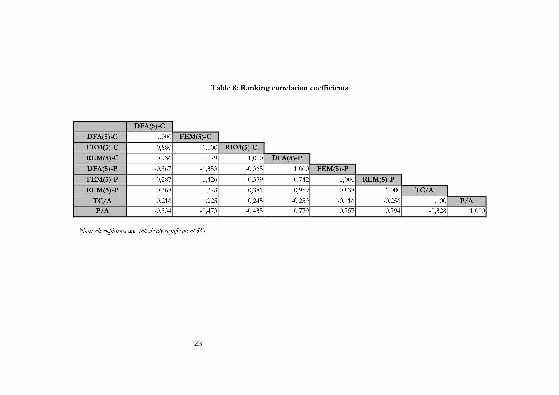
Using the values of efficiency at 5% truncation, the rank correlation coefficients of the
cost and profit efficiencies in table 8 show completely different results. Thus, the coefficient of
rank correlation among the two definitions of efficiency is negative and statistically significant,
whatever the frontier technique used21. The explanation of this result, at first sight contradictory,
is that cost efficiency may be negatively correlated to profit efficiency if the banks which incur the
greatest cost inefficiencies compensate these with higher revenues. This finding can reflect the fact
that banks with the highest revenues feel less pressure from competition to reduce their costs, or
that banks compete in different market segments and provide different product qualities.
One of the indicators of consistency proposed by Bauer et al. (1998) is based on a
comparison of the efficiency indicators and the well known accounting ratios. Table 8 also
contains the rank correlation between cost and profit efficiency on the one hand, and two of the
most frequently used accounting indicators: average costs per unit of assets (TC/A) and the return
on assets (B/A). The most outstanding results are:
1.- The rank correlation of average costs and the estimated cost efficiency is positive and
significant, regardless of the frontier approach used. Thus, paradoxically, the most cost-
efficient banks have the highest average costs. This result may be due to the fact that the
accounting ratios do not take into account the differences in the composition of output or
the price of inputs. On the contrary, cost efficiency does take into consideration these
variables because it estimates a cost function including the vector of production and input
prices.
2.- In the case of profit efficiency and ROA, the results confirm the expected sign. There
is a high positive correlation between the two indicators, so that those banks that achieve
the highest levels of profit efficiency are the most profitable22.
21 The most paradoxical case is the United Kingdom, the second most inefficient country in costs and the mostefficient one in profits.22 At the aggregate level, there is an exact coincidence between the most profit efficient sector and the sectorwith the highest return on assets. Thus, the UK enjoys the highest profitability and the highest profitefficiency.
23
7DEOH �� 5DQNLQJ FRUUHODWLRQ FRHIILFLHQWV
')$����&
')$����& ����� )(0����&
)(0����& ����� ����� 5(0����&
5(0����& ����� ����� ����� ')$����3
')$����3 ������ ������ ������ ����� )(0����3
)(0����3 ������ ������ ������ ����� ����� 5(0����3
5(0����3 ������ ������ ������ ����� ����� ����� 7&�$
7&�$ ����� ����� ����� ������ ������ ������ ����� 3�$
3�$ ������ ������ ������ ����� ����� ����� ������ �����
1RWH� DOO FRHIILFLHQWV DUH VWDWLVWLFDOO\ VLJQLILFDQW DW ��
24
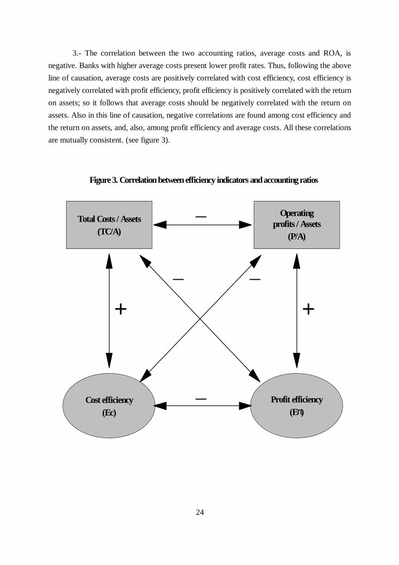
3.- The correlation between the two accounting ratios, average costs and ROA, is
negative. Banks with higher average costs present lower profit rates. Thus, following the above
line of causation, average costs are positively correlated with cost efficiency, cost efficiency is
negatively correlated with profit efficiency, profit efficiency is positively correlated with the return
on assets; so it follows that average costs should be negatively correlated with the return on
assets. Also in this line of causation, negative correlations are found among cost efficiency and
the return on assets, and, also, among profit efficiency and average costs. All these correlations
are mutually consistent. (see figure 3).
Figure 3. Correlation between efficiency indicators and accounting ratios
Total Costs / Assets(TC/A)
Operating profits / Assets
(P/A)
Cost efficiency(Ec)
++
Profit efficiency(E )π
25
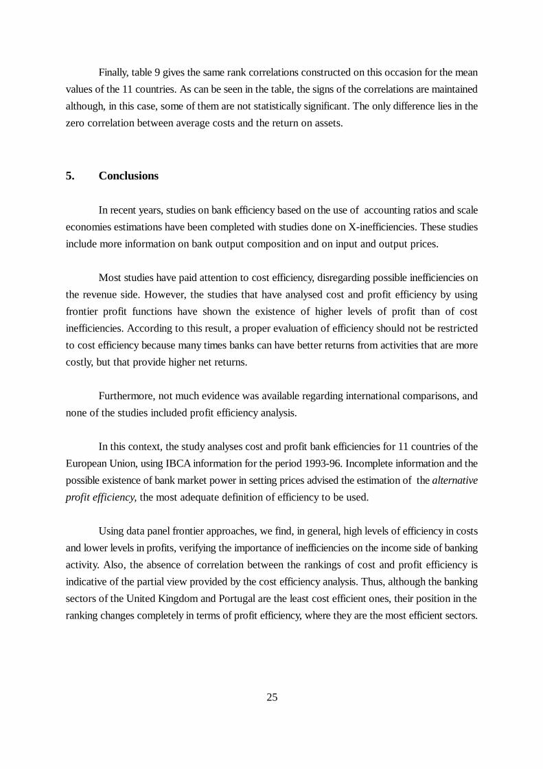
Finally, table 9 gives the same rank correlations constructed on this occasion for the mean
values of the 11 countries. As can be seen in the table, the signs of the correlations are maintained
although, in this case, some of them are not statistically significant. The only difference lies in the
zero correlation between average costs and the return on assets.
5. Conclusions
In recent years, studies on bank efficiency based on the use of accounting ratios and scale
economies estimations have been completed with studies done on X-inefficiencies. These studies
include more information on bank output composition and on input and output prices.
Most studies have paid attention to cost efficiency, disregarding possible inefficiencies on
the revenue side. However, the studies that have analysed cost and profit efficiency by using
frontier profit functions have shown the existence of higher levels of profit than of cost
inefficiencies. According to this result, a proper evaluation of efficiency should not be restricted
to cost efficiency because many times banks can have better returns from activities that are more
costly, but that provide higher net returns.
Furthermore, not much evidence was available regarding international comparisons, and
none of the studies included profit efficiency analysis.
In this context, the study analyses cost and profit bank efficiencies for 11 countries of the
European Union, using IBCA information for the period 1993-96. Incomplete information and the
possible existence of bank market power in setting prices advised the estimation of the alternative
profit efficiency, the most adequate definition of efficiency to be used.
Using data panel frontier approaches, we find, in general, high levels of efficiency in costs
and lower levels in profits, verifying the importance of inefficiencies on the income side of banking
activity. Also, the absence of correlation between the rankings of cost and profit efficiency is
indicative of the partial view provided by the cost efficiency analysis. Thus, although the banking
sectors of the United Kingdom and Portugal are the least cost efficient ones, their position in the
ranking changes completely in terms of profit efficiency, where they are the most efficient sectors.
26
7DEOH �� 5DQNLQJ FRUUHODWLRQ FRHIILFLHQWV �E\ &RXQWULHV�
')$����&
')$����& ����� )(0����&
)(0����& ����� ����� 5(0����&
5(0����& ����� ����� ����� ')$����%
')$����% ������ ������ ������ ����� )(0����%
)(0����% ������ ������ ������ ����� ����� 5(0����%
5(0����% ������ ������ ������ ����� ����� ����� 7&�$
7&�$ ����� ����� ����� ����� ����� ����� ����� 3�$
3�$ ������ ������ ������ ����� ����� ����� ������ �����
6LJQLILFDQW DW � �
6LJQLILFDQW DW � �
6LJQLILFDQW DW �� �
27
The analysis allows us to conclude that average cost levels are not illustrative of cost
efficiency (in fact the rank correlation coefficient is positive) but that they do have the expected
negative effect on profit efficiency. Furthermore, the high levels of average costs affect the
accounting indicator of profit (ROA) negatively. Finally, the correlation of ranks between ROA
and profit efficiency is positive, as was to be expected, and, in this case, with no paradoxical
effect. Consequently, it is possible that the effects of specialisation on costs may be greater than
that on profits.
In view of these results, it can be concluded that the differences of efficiency among the
banks and among the banking sectors considered are not as great as accounting indicators would
indicate. Nor are they as small as suggested by the indices of cost efficiency. There is a notably
wide range of variation in profit efficiency. Actually, it is greater if we take into account that,
although we have worked with individual data, we are presenting average results for countries.
Consequently, it would be interesting to analyse, in coming years, the changes that may occur in
this range of relative efficiencies, as the forces of competition in the new European scenario take
full effect.
28
References
Akhavein, J.D.; Berger, A.N. and Humphrey, D.B. (1997): “The effects of bank megamergers onefficiency and prices: evidence from the profit function”, Review of IndustrialOrganization 12, 95-139.
Allen, L. and Rai, A. (1996): “Operational efficiency in banking: An international comparison”.Journal of Banking and Finance 20, 655-672.
Battese, G.E. and Coelli, T.J. (1988): “Prediction of firm-level efficiencies with a generalizedfrontier production function and panel data”, Journal of Econometrics 38, 387-399.
Bauer, P.W.; Berger, A.N.; Ferrier, G.D. and Humphrey, D.B. (1998): “Consistency conditionsfor regulatory analysis of financial institutions: a comparison of frontier efficiencymethods”, Journal of Economics and Business, forthcoming.
Berger, A.N. and Humphrey, D.B. (1991): "The dominance of inefficiencies over scale andproduct mix economies in banking", Journal of Monetary Economics 28, pp. 117- 148.
Berger, A.N. and Humphrey, D.B. (1992): “Measurement and efficiency issues in commercialbanking”, pp. 24--79 in Z. Griliches, ed., Output Measurement in the service sectors,National Bureau of Economic Research, Studies in Income and Wealth, vol. 56, Chicago:University of Chicago Press.
Berger, A.N.; Nancock, D. and Humphrey, D.B. (1993): “Bank efficiency derived from the profitfunction”, Journal of Banking and Finance 17, 317-347.
Berger, A.N. and Mester, L.J. (1997): “Inside the black box: What explains differences in theefficiencies of financial institutions”, Journal of Banking and Finance 21, 895-947.
Berger, A.N. and Humphrey, D.B. (1997): “Efficiency of financial institutions: internationalsurvey and directions for future research”, European Journal of Operational Research 98,175-212.
DeYoung, R. and Nole, D. (1996): “Foreign-owned banks in the US: earning market share orbuying it?, Journal of Money, Credit and Banking, 28, 622-636.
DeYoung, R. and Hasan, I. (1998): “The performance of the novo commercial banks: a profitefficiency approach”, Journal of Banking and Finance, 22, 565-587.
Fecher, F. and Pestier, P. (1993): “Efficiency and competition in OECD Financial services”, inH.O. Fried, C.A.K. Lovell and S.S. Schmidt (eds.), The Measurement of ProductiveEfficiency: Techniques and Applications, Oxford University Press, Oxford, 374-385.
Humphrey, D.B. and Pulley, L. (1997): “Banks responses to deregulation: profits technology andefficiency”, Journal of Money, Credit and Banking, 73-93.
29
IBCA (Ltd.)., Eldon House, Eldom Street London EC2m 7LS.
Lozano, A. (1997): “Profit efficiency for Spanish savings banks”, European Journal ofOperational Research, 98, 381-394.
Miller, S.M. and Noulas, A.G. (1996): “The technical efficiency of large bank production”,Journal of Banking and Finance, 20, 495-509.
OECD (1997): Bank Profitability. Financial Statements of Banks. 1997.
Pastor, J.M.; Pérez, F. and Quesada, J. (1997): “Efficiency analysis in banking firms: aninternational comparison”, European Journal of Operational Research, vol. 98, Num. 2,395-407.
Rogers, K.E. (1998): “Nontraditional activities and the efficiency of US commercial banks”,Journal of Banking and Finance, 22, 467-482.
Ruthenberg, D. and R. Elias (1996): “Cost economies and interest rate margins in a unifiedEuropean banking market”, Journal of Economics and Business 48, 231-249.
Schmidt, P. and Sickles, R.C. (1984): “Production frontiers and panel data”, Journal of Bussinesand Economic Statistics 2, 367-374.
Simar, (1992): “Estimating efficiencies from frontier models with panel data: a comparison ofparametric, non-parametric and semi-parametric methods with bootstrapping”, Journalof Productivity Analysis, 3, 171-203.