Embed Size (px)
Citation preview

CS 1674: Intro to Computer Vision
Feature Matching and Indexing
Prof. Adriana KovashkaUniversity of Pittsburgh
September 26, 2016
HW3P post-mortem
• Matlab: 21% of you reviewed 0-33% of it
– Please review the entire tutorial ASAP
• How long did HW3P take? (Answer on Socrative)
• What did you learn from it?
• What took the most time?
Plan for Today
• Feature detection (wrap-up)
• Matching features
• Indexing features
– Visual words
• Application to image retrieval
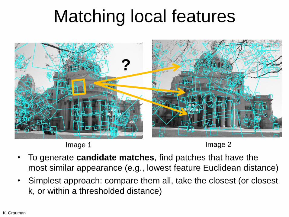
Matching local features
?
• To generate candidate matches, find patches that have the
most similar appearance (e.g., lowest feature Euclidean distance)
• Simplest approach: compare them all, take the closest (or closest
k, or within a thresholded distance)
Image 1 Image 2
K. Grauman
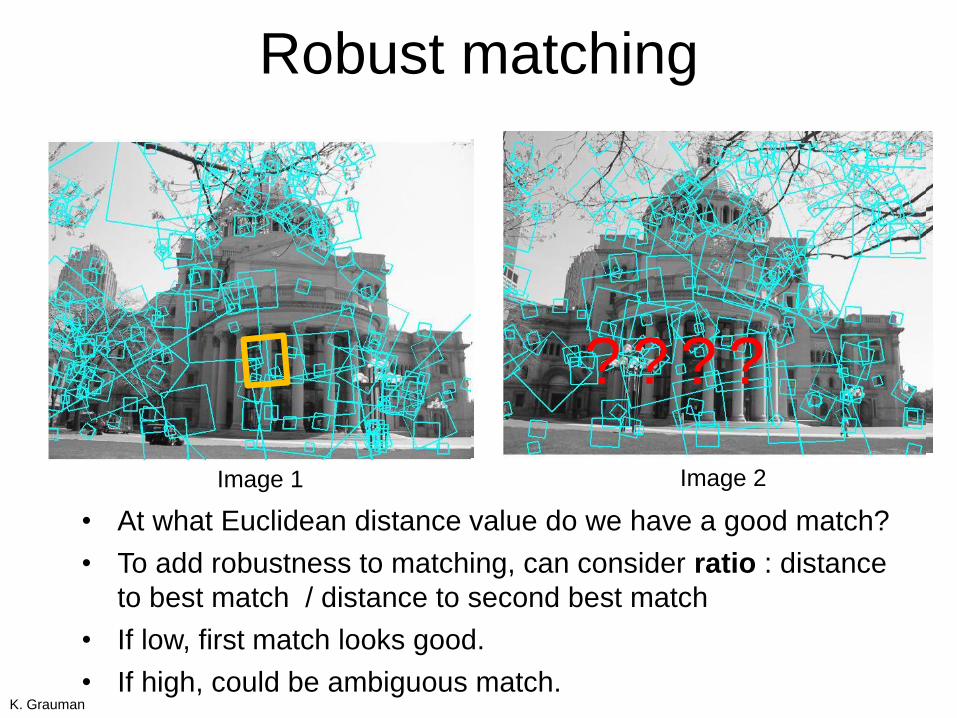
Robust matching
• At what Euclidean distance value do we have a good match?
• To add robustness to matching, can consider ratio : distance
to best match / distance to second best match
• If low, first match looks good.
• If high, could be ambiguous match.
Image 1 Image 2
? ? ? ?
K. Grauman
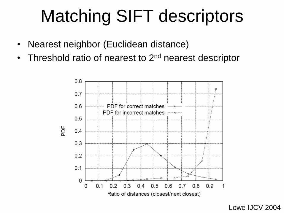
Matching SIFT descriptors
• Nearest neighbor (Euclidean distance)
• Threshold ratio of nearest to 2nd nearest descriptor
Lowe IJCV 2004
• So far we discussed matching across just
two images
• What if you wanted to match a query
feature from one image, to all frames in a
video, or to a giant database?
• With potentially thousands of features per
image, and hundreds to millions of images
to search, how to efficiently find those that
are relevant to a new image?
Efficient matching
Adapted from K. Grauman
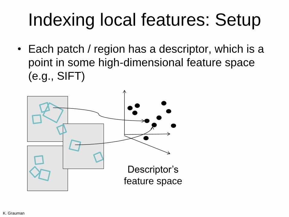
Indexing local features: Setup
• Each patch / region has a descriptor, which is a
point in some high-dimensional feature space
(e.g., SIFT)
Descriptor’s
feature space
K. Grauman
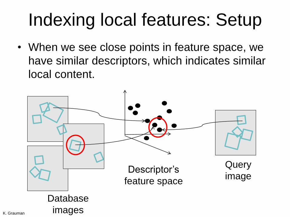
Indexing local features: Setup
• When we see close points in feature space, we
have similar descriptors, which indicates similar
local content.
Descriptor’s
feature space
Database
images
Query
image
K. Grauman
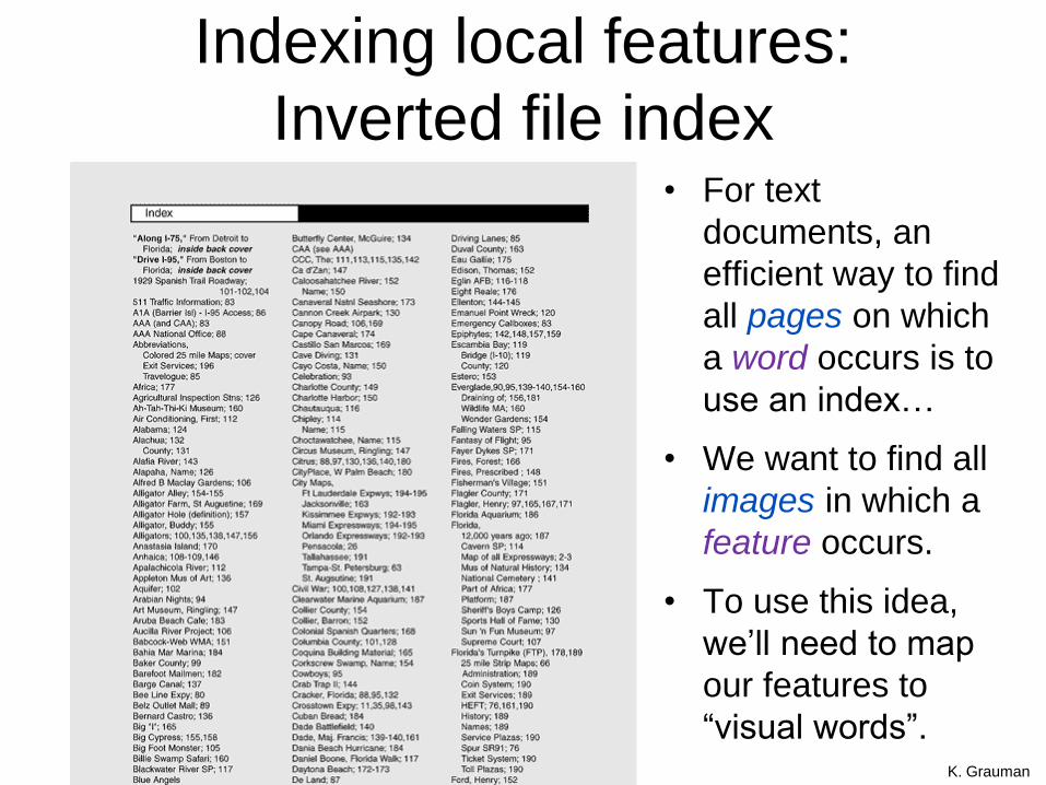
Indexing local features:
Inverted file index• For text
documents, an
efficient way to find
all pages on which
a word occurs is to
use an index…
• We want to find all
images in which a
feature occurs.
• To use this idea,
we’ll need to map
our features to
“visual words”.K. Grauman
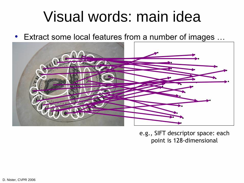
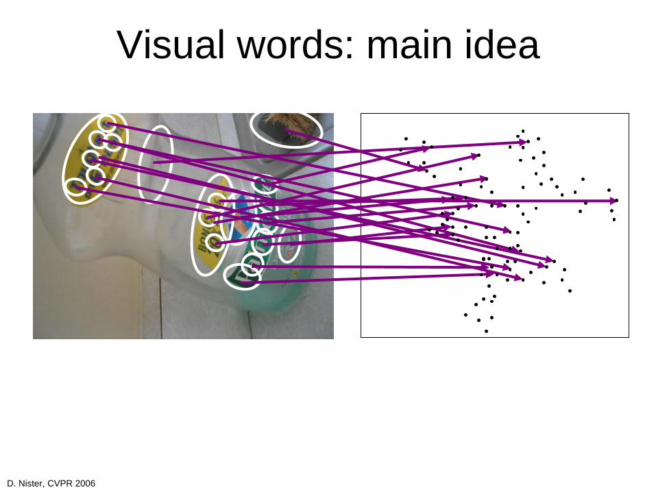
Visual words: main idea
• Extract some local features from a number of images …
e.g., SIFT descriptor space: each
point is 128-dimensional
D. Nister, CVPR 2006
Visual words: main idea
D. Nister, CVPR 2006
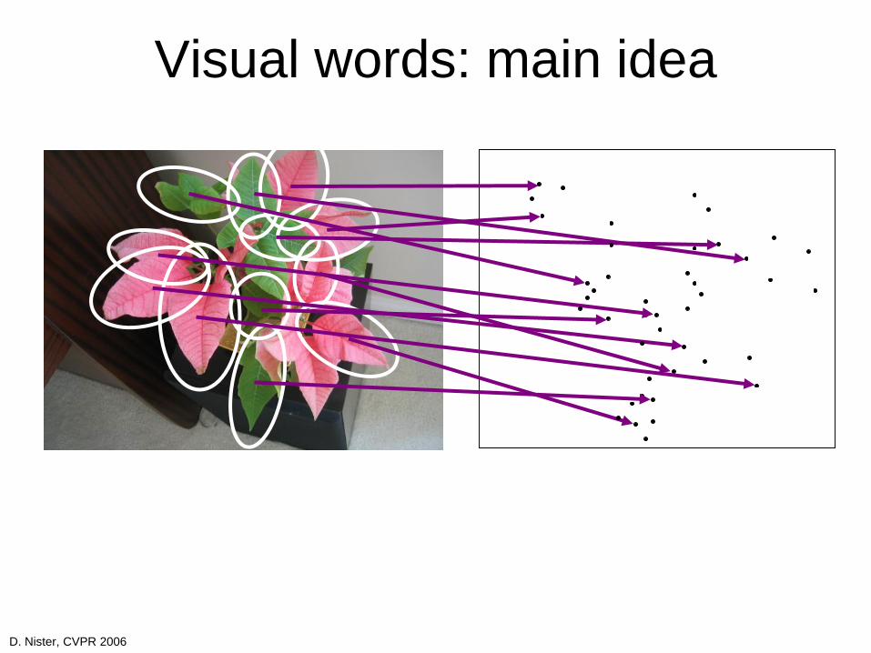
Visual words: main idea
D. Nister, CVPR 2006
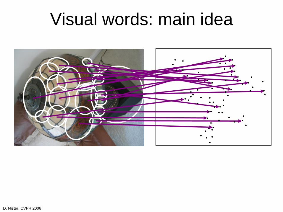
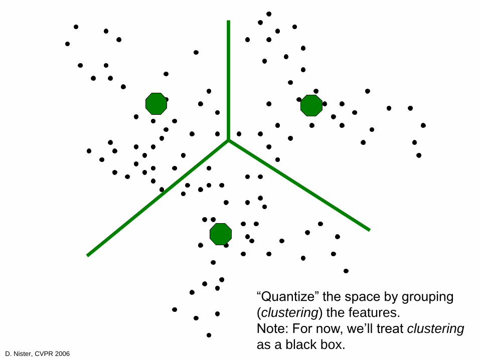
Visual words: main idea
D. Nister, CVPR 2006
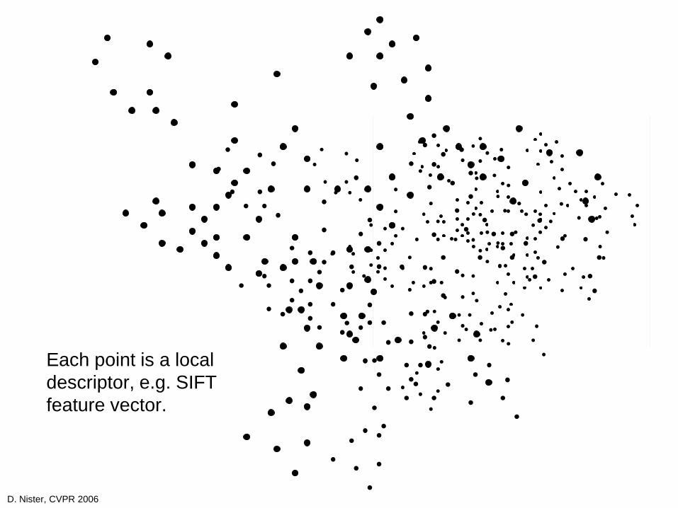
Each point is a local
descriptor, e.g. SIFT
feature vector.
D. Nister, CVPR 2006
D. Nister, CVPR 2006
“Quantize” the space by grouping
(clustering) the features.
Note: For now, we’ll treat clustering
as a black box.
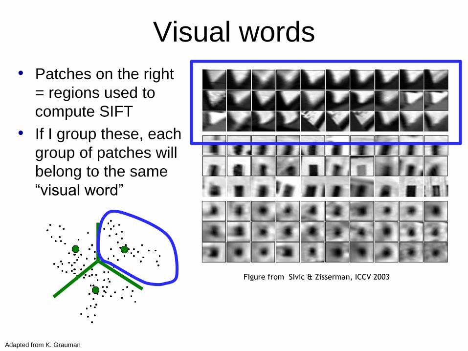
• Patches on the right
= regions used to
compute SIFT
• If I group these, each
group of patches will
belong to the same
“visual word”
Figure from Sivic & Zisserman, ICCV 2003
Adapted from K. Grauman
Visual words
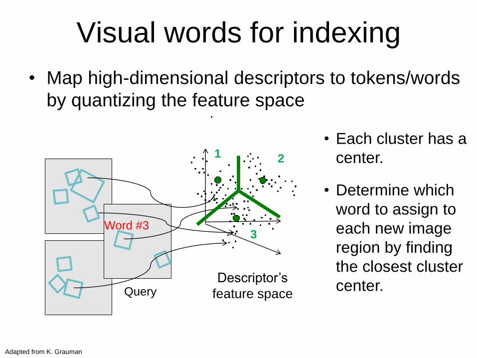
Visual words for indexing
• Map high-dimensional descriptors to tokens/words
by quantizing the feature space
Descriptor’s
feature space
• Each cluster has a
center.
• Determine which
word to assign to
each new image
region by finding
the closest cluster
center.
Word #3
Adapted from K. Grauman
Query
1 2
3
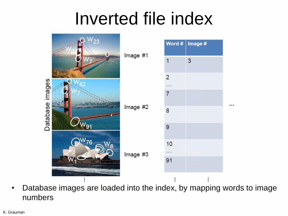
Inverted file index
• Database images are loaded into the index, by mapping words to image
numbers
K. Grauman
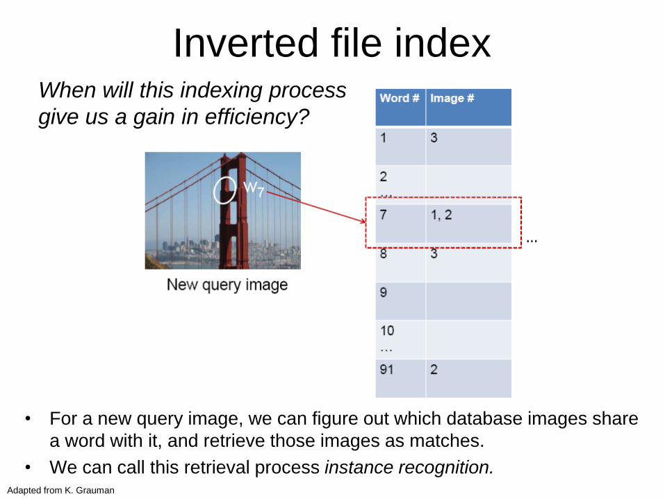
• For a new query image, we can figure out which database images share
a word with it, and retrieve those images as matches.
• We can call this retrieval process instance recognition.
Inverted file indexWhen will this indexing process
give us a gain in efficiency?
Adapted from K. Grauman
Of all the sensory impressions proceeding to
the brain, the visual experiences are the
dominant ones. Our perception of the world
around us is based essentially on the
messages that reach the brain from our eyes.
For a long time it was thought that the retinal
image was transmitted point by point to visual
centers in the brain; the cerebral cortex was a
movie screen, so to speak, upon which the
image in the eye was projected. Through the
discoveries of Hubel and Wiesel we now
know that behind the origin of the visual
perception in the brain there is a considerably
more complicated course of events. By
following the visual impulses along their path
to the various cell layers of the optical cortex,
Hubel and Wiesel have been able to
demonstrate that the message about the
image falling on the retina undergoes a step-
wise analysis in a system of nerve cells
stored in columns. In this system each cell
has its specific function and is responsible for
a specific detail in the pattern of the retinal
image.
sensory, brain,
visual, perception,
retinal, cerebral cortex,
eye, cell, optical
nerve, image
Hubel, Wiesel
China is forecasting a trade surplus of $90bn
(£51bn) to $100bn this year, a threefold
increase on 2004's $32bn. The Commerce
Ministry said the surplus would be created by
a predicted 30% jump in exports to $750bn,
compared with a 18% rise in imports to
$660bn. The figures are likely to further
annoy the US, which has long argued that
China's exports are unfairly helped by a
deliberately undervalued yuan. Beijing
agrees the surplus is too high, but says the
yuan is only one factor. Bank of China
governor Zhou Xiaochuan said the country
also needed to do more to boost domestic
demand so more goods stayed within the
country. China increased the value of the
yuan against the dollar by 2.1% in July and
permitted it to trade within a narrow band, but
the US wants the yuan to be allowed to trade
freely. However, Beijing has made it clear that
it will take its time and tread carefully before
allowing the yuan to rise further in value.
China, trade,
surplus, commerce,
exports, imports, US,
yuan, bank, domestic,
foreign, increase,
trade, value
ICCV 2005 short course, L. Fei-Fei
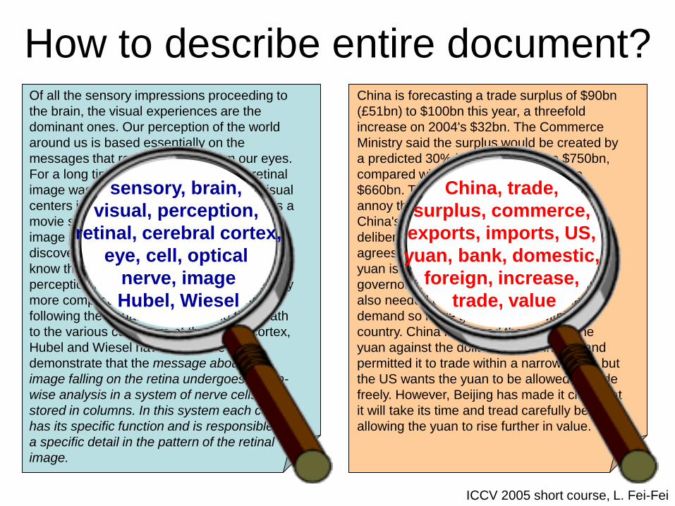
How to describe entire document?
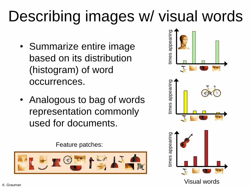
• Summarize entire image
based on its distribution
(histogram) of word
occurrences.
• Analogous to bag of words
representation commonly
used for documents.
Describing images w/ visual words
tim
es a
pp
ea
rin
g
tim
es a
pp
ea
rin
g
tim
es a
pp
ea
rin
g
Feature patches:
Visual wordsK. Grauman
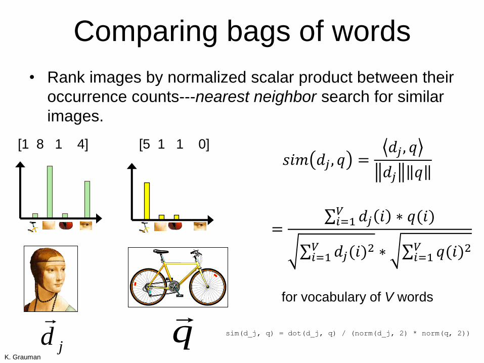
Comparing bags of words
• Rank images by normalized scalar product between their
occurrence counts---nearest neighbor search for similar
images.
[5 1 1 0][1 8 1 4]
jd
q
𝑠𝑖𝑚 𝑑𝑗 , 𝑞 =𝑑𝑗 , 𝑞
𝑑𝑗 𝑞
= 𝑖=1𝑉 𝑑𝑗 𝑖 ∗ 𝑞(𝑖)
𝑖=1𝑉 𝑑𝑗(𝑖)
2 ∗ 𝑖=1𝑉 𝑞(𝑖)2
for vocabulary of V words
K. Grauman
sim(d_j, q) = dot(d_j, q) / (norm(d_j, 2) * norm(q, 2))
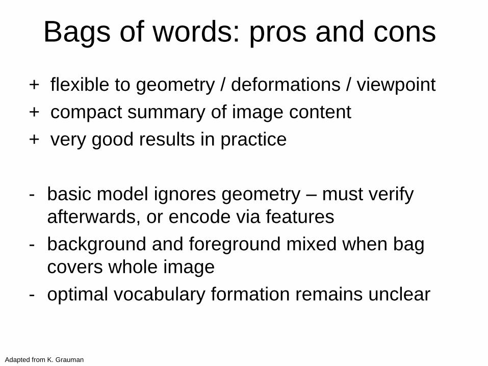
Bags of words: pros and cons
+ flexible to geometry / deformations / viewpoint
+ compact summary of image content
+ very good results in practice
- basic model ignores geometry – must verify
afterwards, or encode via features
- background and foreground mixed when bag
covers whole image
- optimal vocabulary formation remains unclear
Adapted from K. Grauman
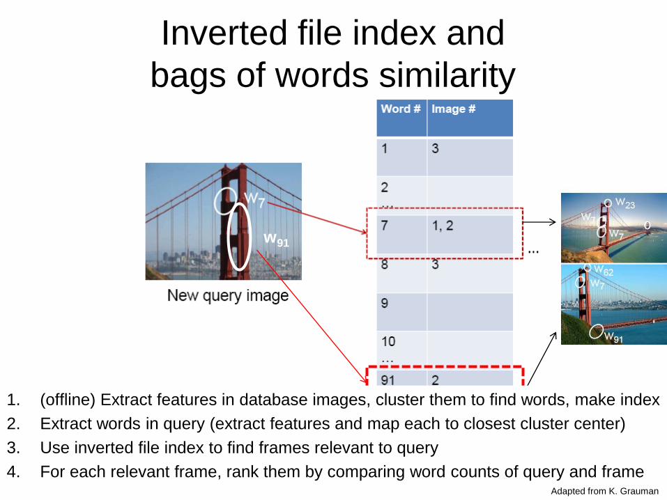
Inverted file index and
bags of words similarity
w91
1. (offline) Extract features in database images, cluster them to find words, make index
2. Extract words in query (extract features and map each to closest cluster center)
3. Use inverted file index to find frames relevant to query
4. For each relevant frame, rank them by comparing word counts of query and frameAdapted from K. Grauman

One more trick: tf-idf weighting
• Term frequency – inverse document frequency
• Describe image/frame by frequency of each word within it,
but downweight words that appear often in the database
• (Standard weighting for text retrieval)
Total number of
documents in
database
Number of documents
in which word i occurs
Number of
occurrences of word
i in document d
Number of words in
document d
Adapted from K. Grauman
Normalized bag-of-words

Slide from Andrew Zisserman
Sivic & Zisserman, ICCV 2003
Bags of words for content-based
image retrieval
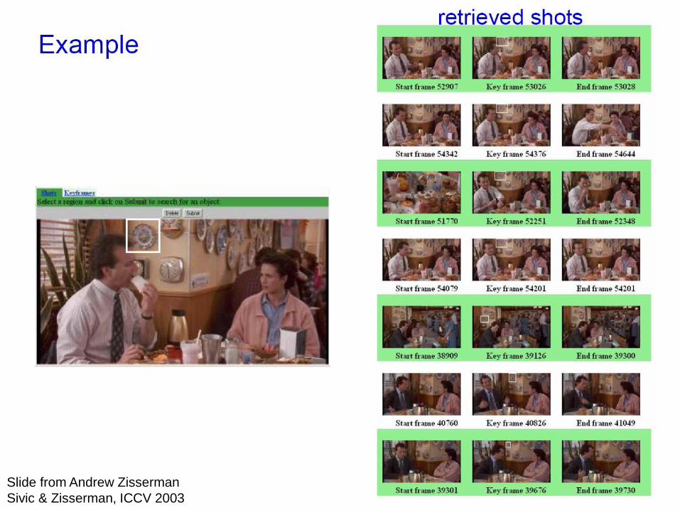
Slide from Andrew Zisserman
Sivic & Zisserman, ICCV 2003
Perc
eptu
al
and S
enso
ry A
ugm
ente
d C
om
puti
ng
Vis
ual
Ob
ject
Reco
gn
itio
n T
uto
rial
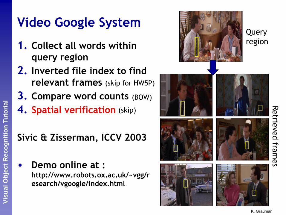
Video Google System
1. Collect all words within
query region
2. Inverted file index to find
relevant frames
3. Compare word counts
4. Spatial verification
Sivic & Zisserman, ICCV 2003
• Demo online at : http://www.robots.ox.ac.uk/~vgg/r
esearch/vgoogle/index.html
Query
region
Retrie
ved fra
mes
K. Grauman
(skip for HW5P)
(BOW)
(skip)

Preview: Spatial Verification
Both image pairs have many visual words in common.
Query Query
DB image with high BoWsimilarity DB image with high BoW
similarity
Ondrej Chum
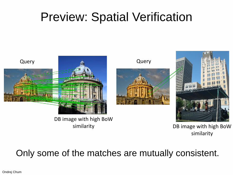
Only some of the matches are mutually consistent.
Preview: Spatial Verification
Query Query
DB image with high BoWsimilarity DB image with high BoW
similarity
Ondrej Chum
Perc
eptu
al
and S
enso
ry A
ugm
ente
d C
om
puti
ng
Vis
ual
Ob
ject
Reco
gn
itio
n T
uto
rial
B. Leibe
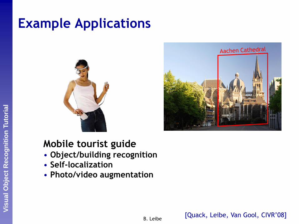
Example Applications
Mobile tourist guide• Object/building recognition
• Self-localization
• Photo/video augmentation
[Quack, Leibe, Van Gool, CIVR’08]
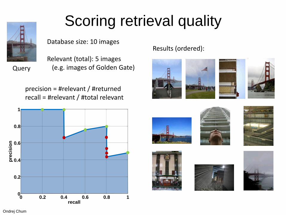
Scoring retrieval quality
0 0.2 0.4 0.6 0.8 10
0.2
0.4
0.6
0.8
1
recall
pre
cis
ion
Query
Database size: 10 images
Relevant (total): 5 images(e.g. images of Golden Gate)
Results (ordered):
precision = #relevant / #returnedrecall = #relevant / #total relevant
Ondrej Chum
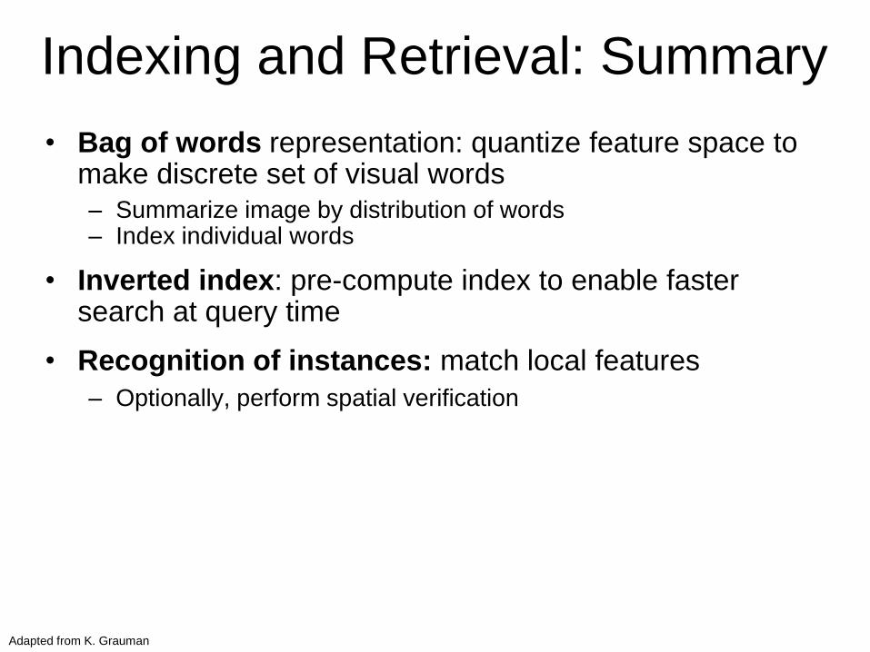
Indexing and Retrieval: Summary
• Bag of words representation: quantize feature space to make discrete set of visual words
– Summarize image by distribution of words– Index individual words
• Inverted index: pre-compute index to enable faster search at query time
• Recognition of instances: match local features
– Optionally, perform spatial verification
Adapted from K. Grauman