Data Warehousing

A data warehouse is a special purpose database. Classic databases are generally used to model some enterprise. Most often they are used to support transactions, a process that is referred to an On-Line Transaction Processing system (OLTP). A data warehouse on the other hand is designed to support decision-making or so-called analytical processing, On-line Analytical Processing (OLAP). The general idea is to prepare data so that useful information can be abstracted from the data via statistical analysis, artificial intelligence or other special purpose techniques. (This last process is called “Data Mining”) MOTIVATING ABSTRACTION: The purpose of a data warehouse is to allow an analyst to view an entire database as if it were one huge spreadsheet.1 Definition:. (Bill Inmon, 1992) A data warehouse is a

subject oriented, integrated, time-varying, non-volatile

collection of data that is used primarily in organizational decision making. We recognize three distinct sub-types: 1.An Operational Data Store (ODS), which is a replicated (OLTP) database, which is used for

summary Analysis. Sometimes it is called a virtual warehouse. It is very easy to build, but requires extra capacity on the operational database servers. 2. A “data mart” is a functionally specialized Data warehouse, which usually contains a subset of all available data (of interest to a specific group of users), although it may be linked to an OLTP DBMS 3. An Enterprise Data Store (EDS) contains information taken from throughout an organization. It is used for cross-departmental analysis, executive information systems and data mining applications.2

A data warehouse should be kept separately from the operational database for both

performance and functional reasons. Performance reasons:

1. The operational database is tuned for transaction processing. Complex OLAP would probable degrade Tx processing considerably

2. Special data organization, access and methods are needed

1.Surajit Chaudhuri and Umeswar Dayal at ICDE 98 Feb 1998.

2 .Gabrielle Gagnon, PC Magazine Mar 9 1999. P 245

Functional reasons: 1. Decision support typically requires historical data, which is not usually kept in an operational

database.. 2.Decision support requires aggregation from multiple heterogeneous sources: the operational

database, external sources, the web etc. 3.Different data sources typically use different data representations, which must be reconciled

before OLAP processing.

The three-tiered architecture:

bottom: database server...usually a relational database. middle: OLAP server...comes in two basic flavors

ROLAP (relational OLAP) is an extension of the relational DBMS that maps multi-dimensional data to standard relational operations. MOLAP (multi-dimensional OLAP): A special purpose server that directly implements multi-dimensional data and operations.

top: Clients: Query and reporting tools Analysis tools Data Mining tools

OLAP Models and Tools

The multi-dimension data model: This model views data in the form of a multidimensional cube. Let’s proceed slowly.

A data cube is defined by dimensions and facts. In general terms dimensions are the entities that the warehouse is interested in observing, and facts are numerical measures. A dimension table consists of the attributes of a particular dimension, and a fact table contains the metrics or numbers of the facts, and some pointers (foreign keys) to the dimension tables. Consider a standard spreadsheet. It is a two-dimensional matrix. For instance, we can consider the dimensions time and item at a particular location of a department store, for the sales in dollars, and create the following two-dimensional cube: item Tables Chairs Lamps time Q1 225 120 540 Q2 200 200 435 Q3 125 120 215 Q4 320 210 555 The dimension table for the dimension item may have some regular attributes, like brand, type, price, etc. Other dimensions, like the time, would not have many attributes. Now if we include the dimension location we can expand the table, so we have a similar table for each one of the locations of the department store – LA, SF, NY. It would be as if we have three planes, each one containing similar information as the one on the table. This will really be a cube. Now we can expand our 3 dimensions to another one, looking at the suppliers for the items – we will have a hypercube – which we may think it is created by using a 3-dimensional cube for each one of the suppliers.

1. A database is a set of facts (points) in a multi-dimensional space. (We can view a tuple in a relational database in this way: the dimensions of the space correspond to the attributes of the relation and the points along the axes to the domain of the attribute.) 2. Each fact has a measurable dimension ... sales amount, budget etc. (in the sports database, a fact in the colleges table has an enrollment dimension.) 3. Each fact has a dimension along which data can be analyzed.... state, store, region, product number etc. 4. Dimensions form a sparsely populated coordinate system. 5. Each dimension has an (set of) attribute(s).

Note: We know that a dimension may consist of multiple attributes. If so they will often be related. Those relationships may be

strictly hierarchical, as in city B> state B> country ( most common ), or form a graph or lattice, as in:

date B> month B> year date B> week B> year

These dependencies influence the choice of operations and data representation.

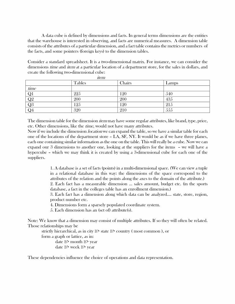
Schemas for Multidimensional Databases. In the design of the relational databases, the entity-relationship data model is normally used. In the design of a data warehouse, a multidimensional model is most appropriated. There are three common multidimensional schemas that are used to generate a multidimensional model: The star schema, the snowflake schema and the fact constellation schema. Star schema: This is the most common schema of the three. It consists of a one large fact table, with no redundancy, and a set of “helper” tables, one for each dimension. Looking at the previous example, we will have a multidimensional table with the sales fact table, on a 3-D expansion, whose structure would be: Fact table Product Quarter Location The Product dimension will be linked to the Product dimension table, containing, for instance, the following attributes Product_ID Product Description Product Name Product Style Product Cost …… The Quarter Table Quarter Year The Location table City State Region Country ……. Snowflake schema: This is a variation of the previous one. Instead of having one table for each dimension, the dimension tables are normalized, and therefore there could be more that one table for some dimensions. In the previous star schema, the Product table could be divided into 2, in the following way: Product_ID Product Name * Product Style

Product Cost …… Product Name Product Description …….. Normalized tables are easier to maintain, and reduce storage needs. On the other hand, this saving of storage space is negligible in comparison with the amount of data that exists in the warehouse, and breaking the dimension table into normalized tables will normally reduce the ability of a general browsing, since more joins would be required to perform some queries. Fact constellation schema: Multiple fact tables may share some dimension tables. It can be thought as a collection of stars schemas (this is the reason for the fact constellation or galaxy schema name). In the previous example you may think that besides the sales fact table, we have a shipping fact table, which shares all the dimension of the sales fact table. Note that the sharing of all the dimension tables is not needed. A fact constellation schema may limit the possible queries for the warehouse. Warehouse indexing. To facilitate the access of data, warehouses utilize indexing techniques, different from the techniques use in the relational databases. We will discuss here the bitmap indexing and the join indexing. Bitmap indexing: This method is the most frequently used in the OLAP products, because it allows a very fast searching on the cubes. The idea is to construct a bit vector for each value in a domain (or column) of the attribute being indexed. So if the domain of a given attribute consists of m values, for instance, we need a vector with m bits for each entry in the bitmap index. For any value of the attribute, we set to 1 the bit representing this value, and to 0 the rest of the bits. Imagine that we have 500,000 cars, and five different categories of car: economy, compact, midsize, full size and luxury. If we want to build a bitmap index for the car size, we will use 2,500,000 bits (5 * 500,000). It is clear that this method works well if the domain of the attribute contains a low number of possible values. Otherwise some compression techniques should be used. This index provides a great improvement for the operations of comparison, aggregation, and joins(see below). Join indexing: This method is based on the ideas of relational databases indexes relating primary keys and foreign keys values. Regular indexing normally relates the values of a dimension of a star schema to rows in the fact table. In traditional indexing the value of a given column is mapped to a list of rows having that

value. In relational databases, a join index keeps track of the joinable rows of two relations. In the star schema, the join indexing is used to maintain the relationship between attribute values of a dimension (primary key in the dimension table) and the corresponding rows in the fact table(foreign key in the fact table). In fact join indices may span multiple dimensions to form composite join indices. Operations in the Multidimensional Data Model:

Aggregation (often called “roll up”) of detailed data to create summary data. -dimension reduction.. 1. Total sales by city 2. Total sales by city by product. Navigation (often called “drill down”) from an aggregate to detail data. Explodes the cube

by unaggregating the data.. Selection defines a sub-cube... If we select along one dimension of the cube (often called

“slicing”) we may have the equivalent of the geometric projection operation along one dimension If we perform a selection on two or more dimensions we will do a “dicing”.

Calculation -within a dimension...e.g. calculate ( sales - expenses ) by office -across dimensions..e.g. divide the cost of advertising for a family of products by

market share of of the individual products...n.b. these numbers exist at different levels of the cube.

Ranking find the top 3% of offices by average income. Visualization. The ability to actually view the data:

- nesting.. View multi-dimensional data in 2 dimensions (like creating a tree using the structure of the data

Jan Feb Mar LA SF NY LA SF NY LA SF NY A B C A B C A B C A B C A B C A B C A B C A B C A B C

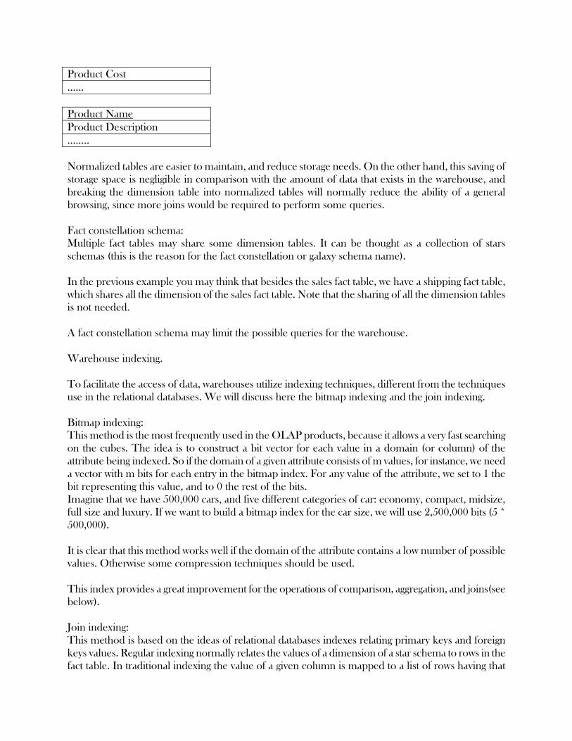
-rotation

Other operations: Some OLAP systems offer additional drilling operations, like drill-across (queries involving more than one fact table) or drill-through (from the bottom level of a data cube down to its back-end relational tables). It also supports functional models for forecasting, trend analysis, and statistical analysis. In this context an OLAP engine is a powerful data analysis tool.

Example: Consider the following multidimensional data model, presented in figure 1. We are going to apply some of the previous operations to that model, to see how the data is presented after each of them. We will always start from the data in figure1.

Figure 1 Multidimensional data model

1) Roll up

When we perform roll up on location (from cities to countries, we obtain the data shown in figure 2. The boxes where the question mark is found indicate that we can’t get the actual data from figure 1. It is straightforward to fill in the values in this boxes, if we supply the missing data to the inner boxes of figure 1.

Figure 2 : Roll up on location

2) Drill down

We are going to drill down on time on the original data. We are going to go from quarters to months.

Figure 3 Drill down on time

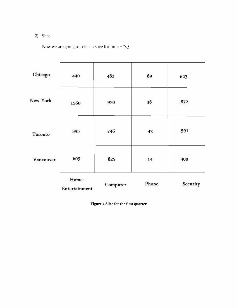
3) Slice

Now we are going to select a slice for time = “Q1”

Figure 4 Slice for the first quarter

4) Dice

In the next figure, we will see the result of the following selection: Dice FOR (location = “Toronto” OR location = “Vancouver”) AND (time = “Q1” OR time = “Q2”) AND (item = “home entertainment” OR item = “computer”

Figure 5 Dice on location, time, and item

5) Nesting

Figure 6 Nesting

6) Combination of operations Our combination of operation is going to be, first to get a slice for time = “Q1”, that gives us

Figure 7 First the slice is performed

Now we rotate (pivot) the slice

Figure 8 Rotated Slice

Many of the operations required for a data warehouse are difficult if not impossible to express

in SQL: 1 Comparisons (with aggregation).

Assume the schema Sales( Sales_id, Store_id, Product_id, amount, date )

Compare last year’s sales with this year’s sales for each product.

Show all sales reps for whom every sale was >= $ 500

Assume the schema Log (Subscriber, log_in time, time_spent)

For each subscriber, find the login time for the longest session Y Select subscriber, max(log_in time) From Log Group By subscriber // ????

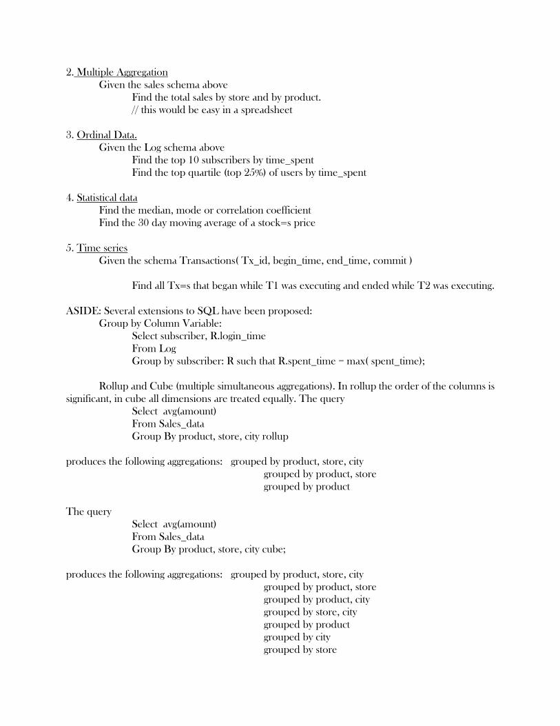
2. Multiple Aggregation Given the sales schema above

Find the total sales by store and by product. // this would be easy in a spreadsheet

3. Ordinal Data.

Given the Log schema above Find the top 10 subscribers by time_spent Find the top quartile (top 25%) of users by time_spent

4. Statistical data

Find the median, mode or correlation coefficient Find the 30 day moving average of a stock=s price

5. Time series

Given the schema Transactions( Tx_id, begin_time, end_time, commit )

Find all Tx=s that began while T1 was executing and ended while T2 was executing. ASIDE: Several extensions to SQL have been proposed:

Group by Column Variable: Select subscriber, R.login_time From Log Group by subscriber: R such that R.spent_time = max( spent_time);

Rollup and Cube (multiple simultaneous aggregations). In rollup the order of the columns is

significant, in cube all dimensions are treated equally. The query Select avg(amount) From Sales_data Group By product, store, city rollup

produces the following aggregations: grouped by product, store, city

grouped by product, store grouped by product

The query

Select avg(amount) From Sales_data Group By product, store, city cube;

produces the following aggregations: grouped by product, store, city

grouped by product, store grouped by product, city grouped by store, city grouped by product grouped by city grouped by store

There are a lot of problems with these operations in order to make sure that the results are still a relation, you have to introduce NULL values into the non-aggregated columns3. Redbrick supplies RISQL that contains a lot of statistical extensions to SQL:

Rank, percentile, moving average, moving sum and dynamic breakpoints Conclusions:

SQL is already too large Extensions will cripple optimizers

END ASIDE

3 Journal of Knowledge and Data Discovery, Vol 1.

Solutions to the OLAP models and tools questions lie now with user-defined, stored procedures or middleware Building the Data Warehouse The Data Warehousing Process.

1. Define Architecture. Do capacity planning 2. Integrate database and OLAP servers, storage and client tools. 3. Design warehouse schema, views 4. Design Physical warehouse organization: data placement, partitioning, access methods 5. Connect sources: gateways, ODBC drivers, wrappers 6. Design and implement scripts for data extraction, loading and refreshing 7. Design metadata and populate repository 8 Design and implement end-user applications 9 Roll out warehouse and applications 10 Manage the warehouse

Step 6. Migrating the data from the ODS.

This is one of the most challenging parts of the process. Issues that must be addressed:

I. Differences in data type. This can occur across products or even within various releases of a single product. Consider the following datatypes for the field “name” from various sources:

Ingres v5 c10 “U of Va ” is the same as “U ofVa ” “MACHINE ” is the same as “MACHINE”

Ingres v5 Char(10) “MACHINE ” is not the same as “MACHINE”

Oracle v6 Char(10) “Jones” Oracle v7 Char(10) “Jones ” will not match.

II. Within one organization, data may be encoded differently in different ODS or in different

parts of the organization...the sex of an employee might be represented as =M=/=F= or 0/1. MISC NOTE: Different systems produce incompatible or inconsistent data. Inmon estimates

that 80% of the time spent building a warehouse would be spent on extracting, cleansing and loading data.