DRA/KV

Decision and Risk Analysis

Financial Modelling & Risk Analysis II

Kiriakos VlahosSpring 2000

DRA/KVSession overview

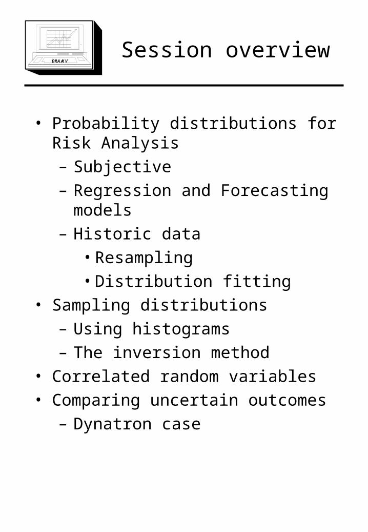
• Probability distributions for Risk Analysis– Subjective– Regression and Forecasting models– Historic data

• Resampling• Distribution fitting

• Sampling distributions– Using histograms– The inversion method

• Correlated random variables• Comparing uncertain outcomes

– Dynatron case

DRA/KV

Using regression models in risk

analysis

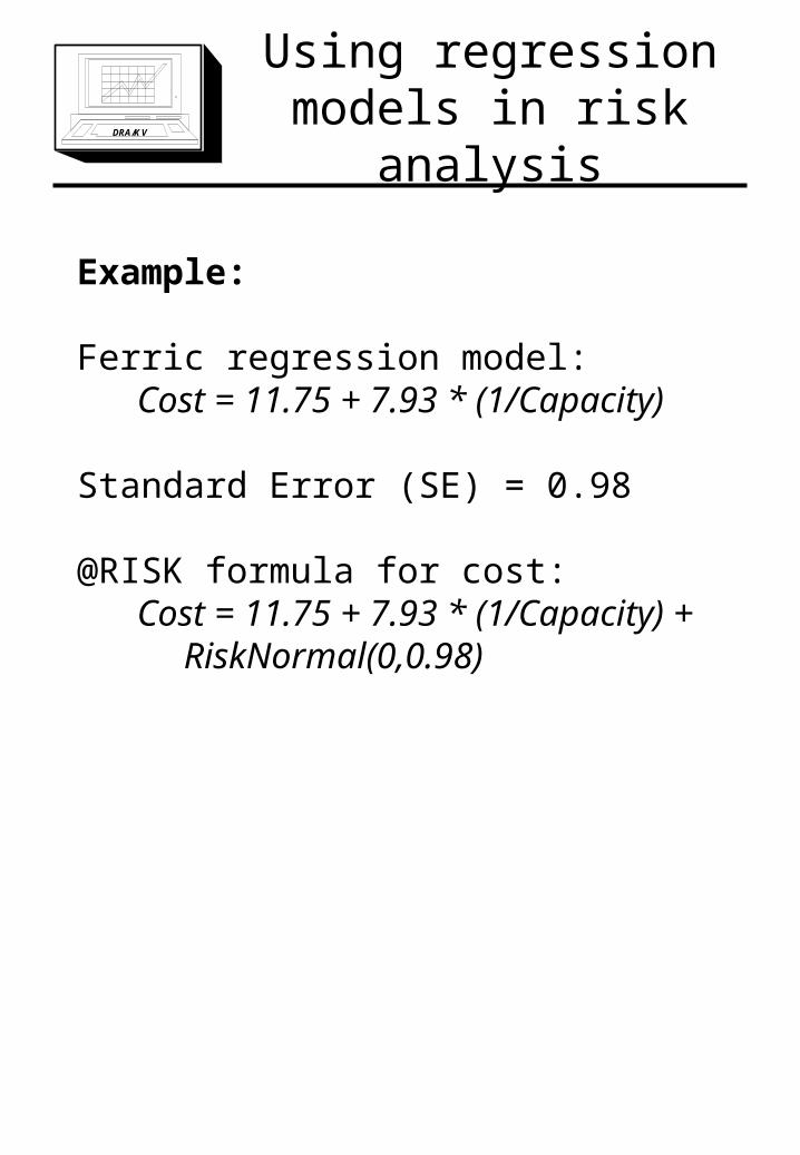
Example:

Ferric regression model:Cost = 11.75 + 7.93 * (1/Capacity)

Standard Error (SE) = 0.98

@RISK formula for cost:Cost = 11.75 + 7.93 * (1/Capacity) +

RiskNormal(0,0.98)

DRA/KV

Using historic dataResampling

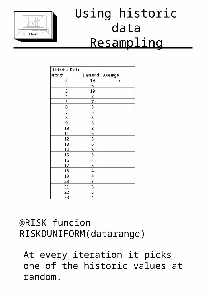
Historical DataMonth Demand Average

1 10 52 63 104 85 76 57 58 59 3

10 211 612 513 614 315 516 417 518 419 420 321 322 323 4

@RISK funcionRISKDUNIFORM(datarange)

At every iteration it picks one of the historic values at random.

DRA/KV

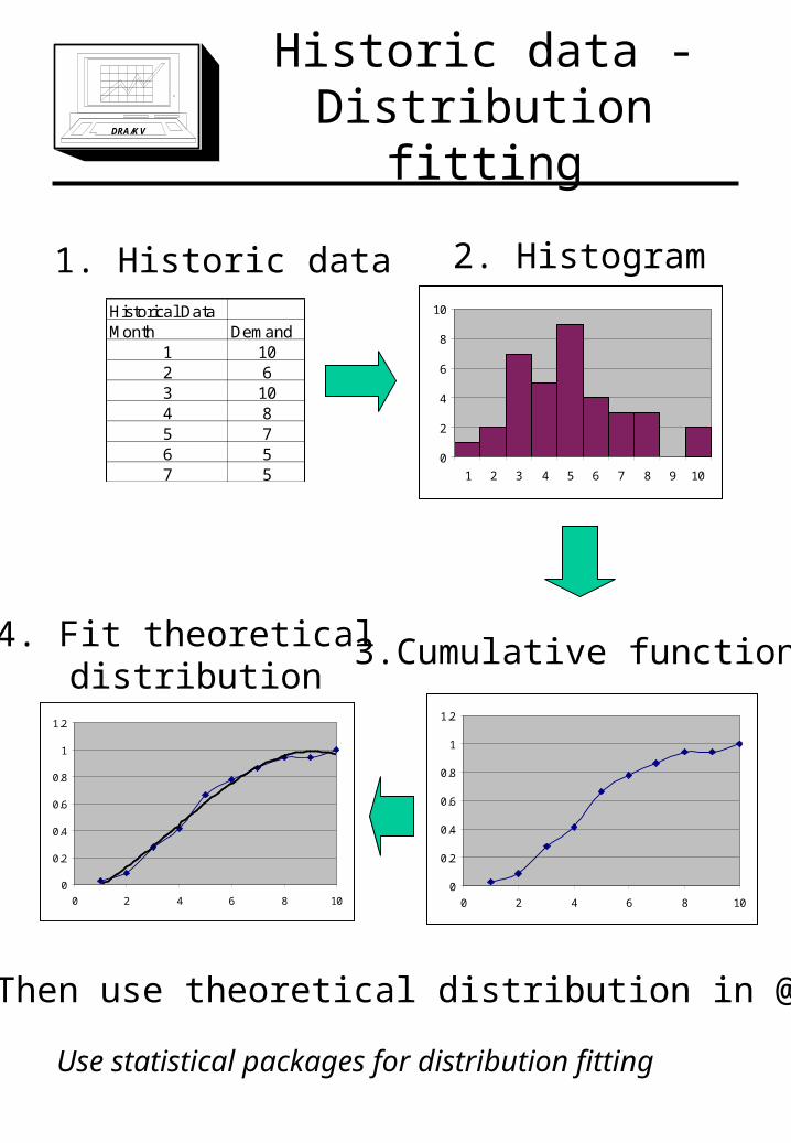
Historic data - Distribution fitting

Historical DataMonth Demand

1 102 63 104 85 76 57 5

1. Historic data

0

2

4

6

8

10

1 2 3 4 5 6 7 8 9 10

2. Histogram

3.Cumulative function

0

0.2

0.4

0.6

0.8

1

1.2

0 2 4 6 8 10

0

0.2

0.4

0.6

0.8

1

1.2

0 2 4 6 8 10

4. Fit theoretical distribution

5. Then use theoretical distribution in @RISK

Use statistical packages for distribution fitting

DRA/KV

Cumulative functions of

standard distributions

Normal(5,1)

0.000

0.200

0.400

0.600

0.800

1.000

-2.27 0.00 2.27 4.54 6.82 9.09 11.36

Normal(5,1)

0.000

0.048

0.095

0.143

0.190

0.238

-2.27 0.00 2.27 4.54 6.82 9.09 11.36

Uniform(1,2)

0.000

0.020

0.040

0.060

0.080

0.100

1.00 1.17 1.33 1.50 1.67 1.83 2.00

Uniform(1,2)

0.000

0.200

0.400

0.600

0.800

1.000

1.00 1.17 1.33 1.50 1.67 1.83 2.00

Triang(1,3,4)

0.000

0.019

0.038

0.058

0.077

0.096

1.00 1.50 2.00 2.50 3.00 3.50 4.00

Triang(1,3,4)

0.000

0.200

0.400

0.600

0.800

1.000

1.00 1.50 2.00 2.50 3.00 3.50 4.00

Distribution function Cumulative function

Uniform

Triangular

Normal

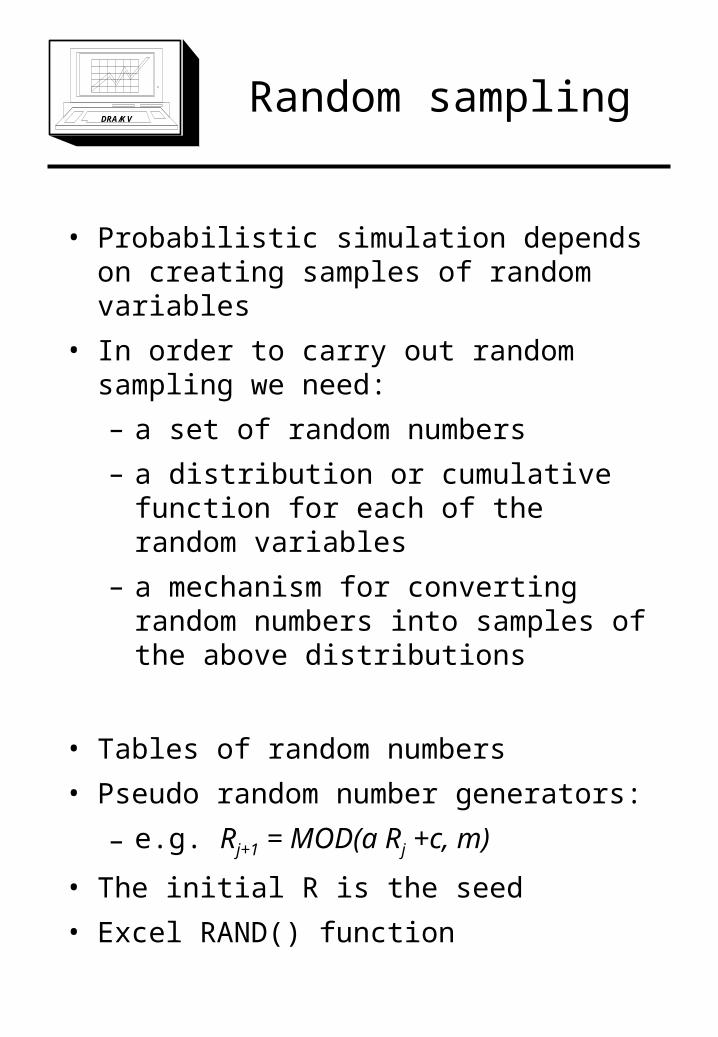
DRA/KVRandom sampling

• Probabilistic simulation depends on creating samples of random variables

• In order to carry out random sampling we need:

– a set of random numbers

– a distribution or cumulative function for each of the random variables

– a mechanism for converting random numbers into samples of the above distributions

• Tables of random numbers

• Pseudo random number generators:

– e.g. Rj+1 = MOD(a Rj +c, m)

• The initial R is the seed

• Excel RAND() function

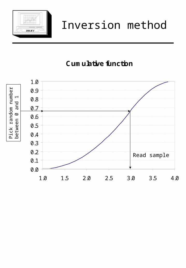
DRA/KVInversion method

Cumulative function

0.0

0.1

0.2

0.3

0.4

0.5

0.6

0.7

0.8

0.9

1.0

1.0 1.5 2.0 2.5 3.0 3.5 4.0

Pic

k ra

ndom

num

ber

betw

een

0 an

d 1

Read sample

DRA/KV

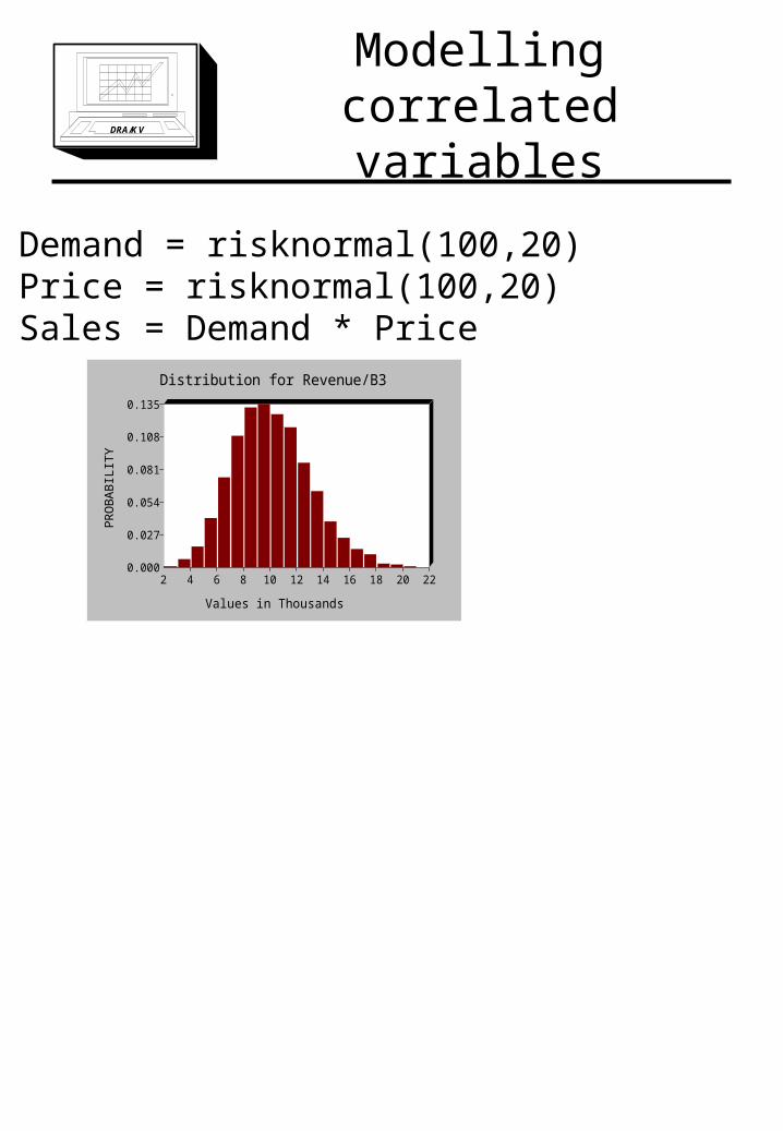
Modelling correlated variables

Demand = risknormal(100,20)Price = risknormal(100,20)Sales = Demand * Price

Distribution for Revenue/B3

PR

OB

AB

ILIT

Y

Values in Thousands

0.000

0.027

0.054

0.081

0.108

0.135

2 4 6 8 10 12 14 16 18 20 22

Assuming correlation of -0.8

Min 2,000Max: 20,500St.d.: 2900

Distribution for Revenue/B3

PR

OB

AB

ILIT

Y

0.000

0.060

0.120

0.180

0.240

0.300

2000 4000 6000 8000 10000120001400016000180002000022000

Min 5,500Max: 13,500St.d.: 1300

Always try to model correlation between random variables

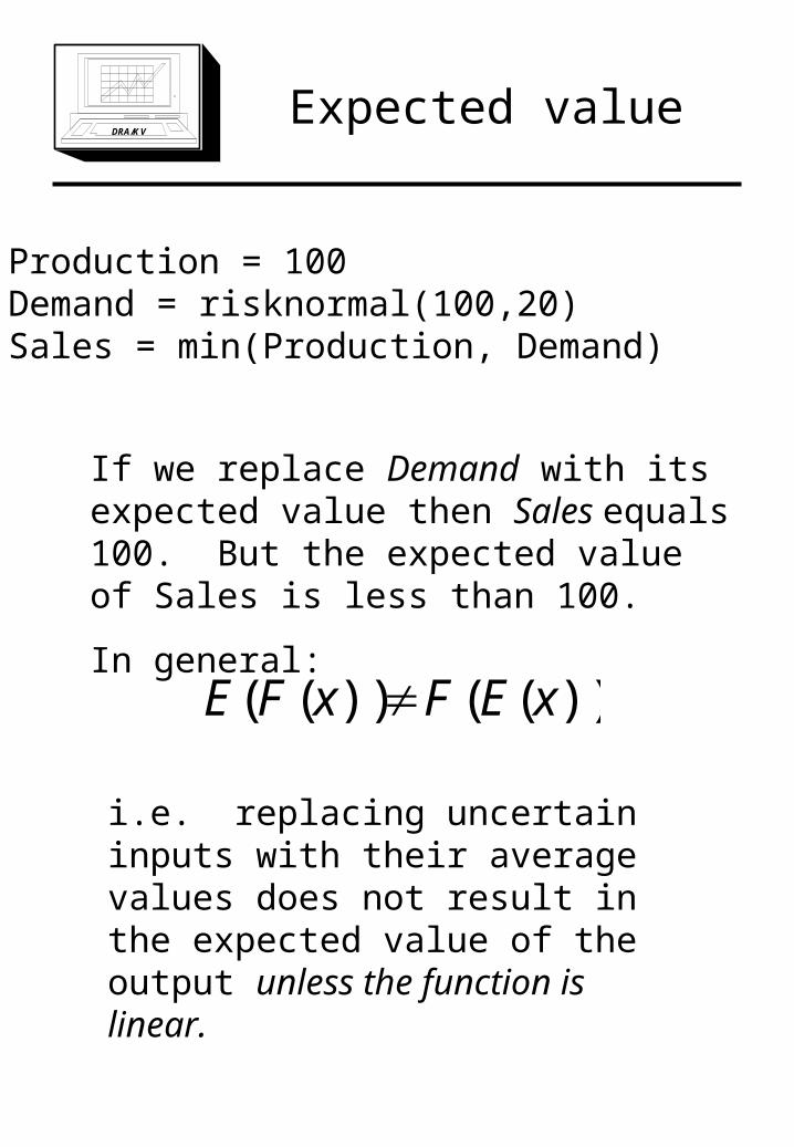
DRA/KVExpected value

Production = 100Demand = risknormal(100,20)Sales = min(Production, Demand)

If we replace Demand with its expected value then Sales equals 100. But the expected value of Sales is less than 100.

In general:

))(())(( xEFxFE

i.e. replacing uncertain inputs with their average values does not result in the expected value of the output unless the function is linear.

DRA/KVDynatron

• Decide about:

– The production level of Dynatron toys

– the split into super and standard

DRA/KV

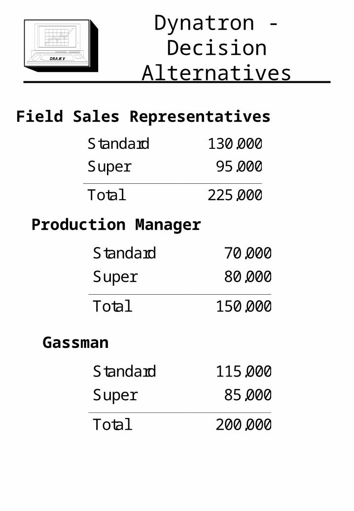
Dynatron - Decision Alternatives

Field Sales Representatives

Production Manager

Standard 70,000

Super 80,000

Total 150,000

Gassman

Standard 115,000

Super 85,000

Total 200,000

Standard 130,000

Super 95,000

Total 225,000

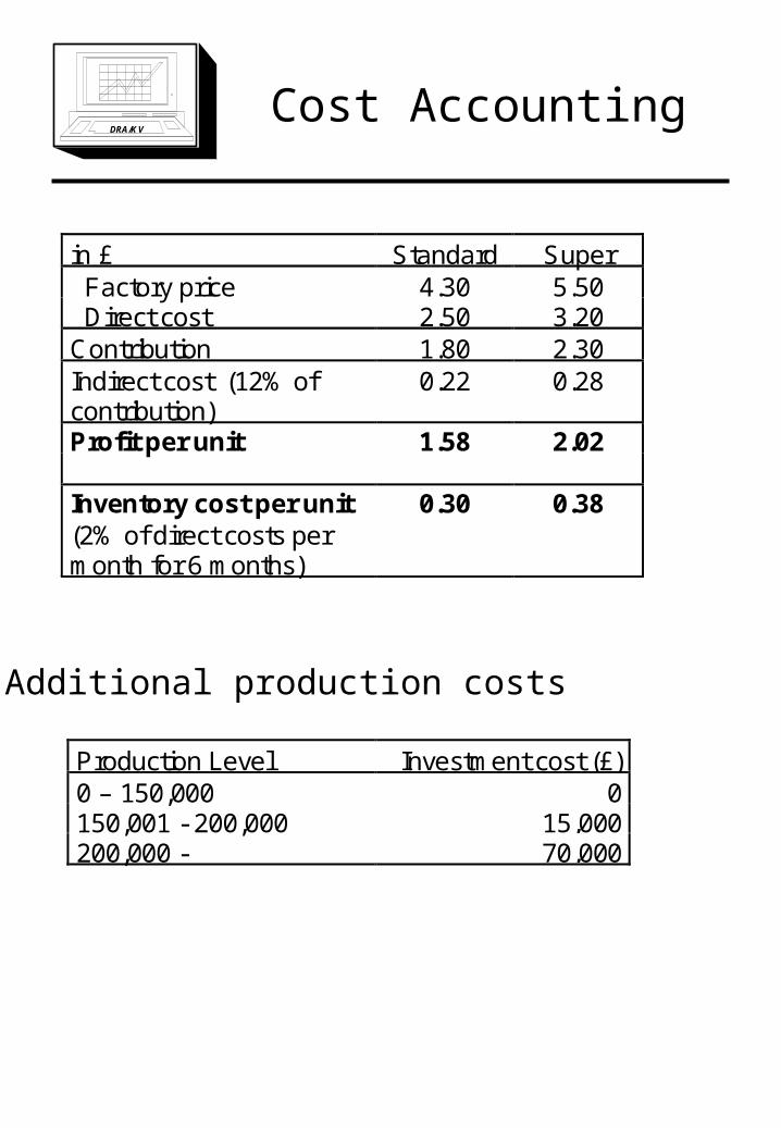
DRA/KVCost Accounting

in £ Standard Super Factory price 4.30 5.50 Direct cost 2.50 3.20Contribution 1.80 2.30Indirect cost (12% ofcontribution)

0.22 0.28

Profit per unit 1.58 2.02

Inventory cost per unit(2% of direct costs permonth for 6 months)

0.30 0.38

Additional production costs

Production Level Investment cost (£)0 – 150,000 0150,001 - 200,000 15,000200,000 - 70,000

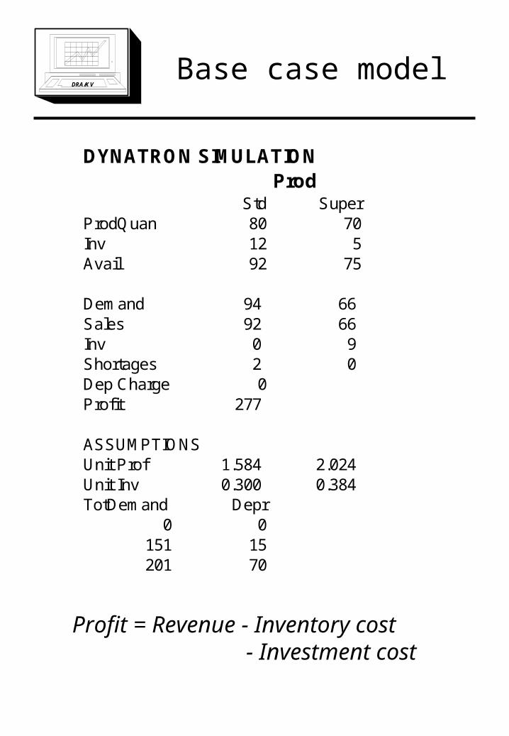
DRA/KVBase case model

DYNATRON SIMULATION Prod

Std SuperProdQuan 80 70Inv 12 5Avail 92 75

Demand 94 66Sales 92 66Inv 0 9Shortages 2 0Dep Charge 0Profit 277

ASSUMPTIONSUnit Prof 1.584 2.024Unit Inv 0.300 0.384TotDemand Depr

0 0151 15201 70

Profit = Revenue - Inventory cost - Investment cost

DRA/KV

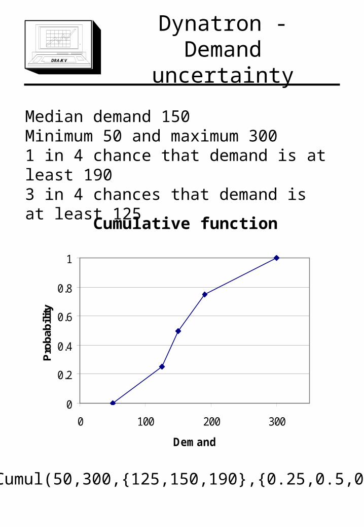
Dynatron - Demand uncertainty

Median demand 150Minimum 50 and maximum 3001 in 4 chance that demand is at least 1903 in 4 chances that demand is at least 125

0

0.2

0.4

0.6

0.8

1

0 100 200 300

Demand

Pro

babi

lity

RiskCumul(50,300,{125,150,190},{0.25,0.5,0.75})

Cumulative function

DRA/KV

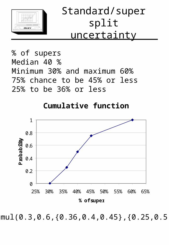
Standard/super split uncertainty

% of supersMedian 40 %Minimum 30% and maximum 60%75% chance to be 45% or less25% to be 36% or less

RiskCumul(0.3,0.6,{0.36,0.4,0.45},{0.25,0.5,0.75})

0

0.2

0.4

0.6

0.8

1

25% 30% 35% 40% 45% 50% 55% 60% 65%

% of super

Pro

ba

bil

ity

Cumulative function

DRA/KV

Dynatron - Simulaton Results

Distribution for Prod/B13P

RO

BA

BIL

ITY

0.000

0.060

0.120

0.180

0.240

0.300

-50 0 50 100 150 200 250 300 350 400

Distribution for Sales/D13

PR

OB

AB

ILIT

Y

0.000

0.060

0.120

0.180

0.240

0.300

-50 0 50 100 150 200 250 300 350 400

Distribution for Gassman/F13

PR

OB

AB

ILIT

Y

0.000

0.060

0.120

0.180

0.240

0.300

-50 0 50 100 150 200 250 300 350 400

DRA/KV

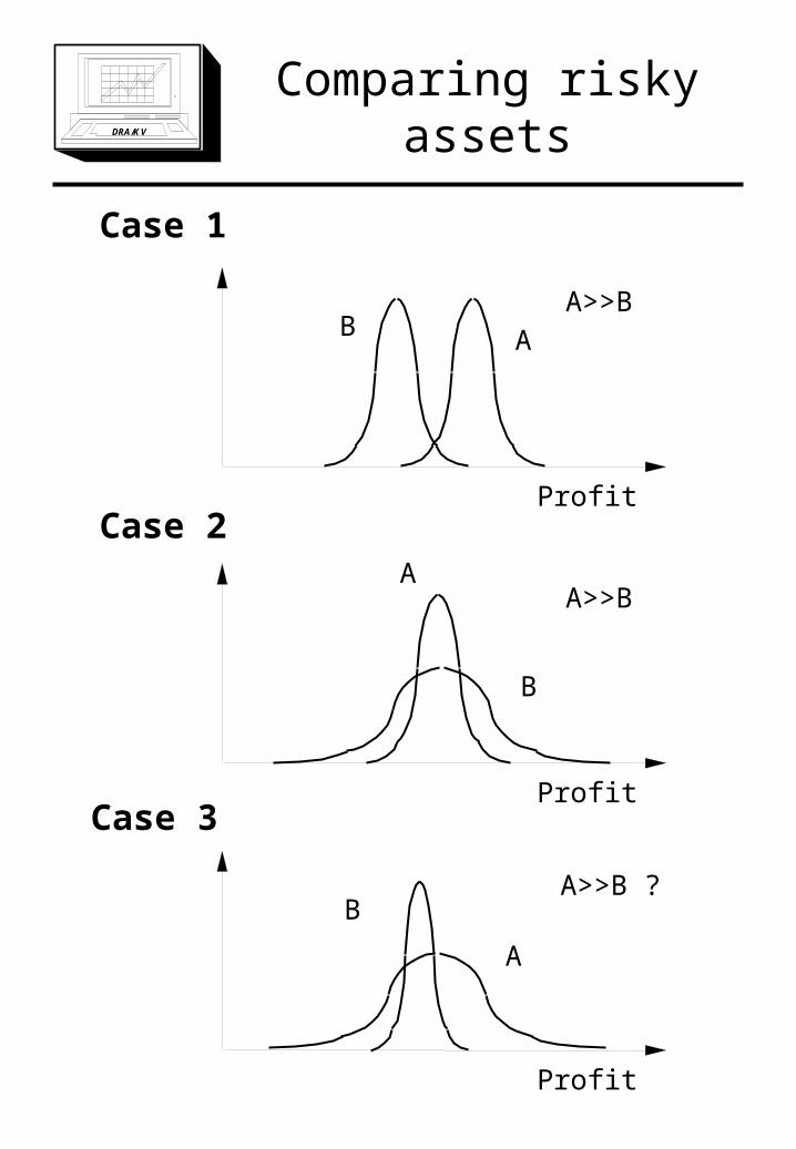
Comparing risky assets

Case 1

B A

Profit

A>>B

Case 2A

B

Profit

A>>B

Case 3

B

A

Profit

A>>B ?

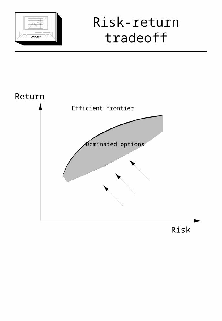
DRA/KVRisk-return tradeoff

Risk

ReturnEfficient frontier

Dominated options

DRA/KV

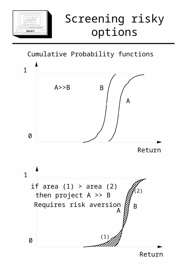
Screening risky options

Return

Cumulative Probability functions

0

1

A

BA>>B

Return

0

1

BA

if area (1) > area (2)

(1)

(2)then project A >> B

Requires risk aversion

DRA/KV

Dynatron - Simulation Results

Gassman and Sales Rep

Prob ofValue <=

X-axisValue

Legends:

0.000

0.200

0.400

0.600

0.800

1.000

-50 0 50 100 150 200 250 300 350 400

F13/ GassmanD13/ Sales

Cumulative probability distributions

Gassman Sales rep.

ExpectedProfit

230 174

St. dev. 97 108

Prob. ofloss

0% 6.5%

DRA/KV

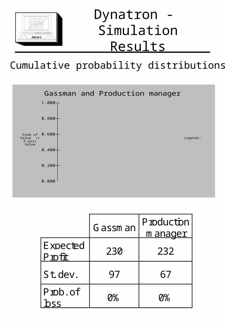
Dynatron - Simulation Results

Cumulative probability distributions

GassmanProductionmanager

ExpectedProfit

230 232

St. dev. 97 67

Prob. ofloss

0% 0%

Gassman and Production manager

Prob ofValue <=

X-axisValue

Legends:

0.000

0.200

0.400

0.600

0.800

1.000

-50 0 50 100 150 200 250 300 350 400

F13/ GassmanB13/ Prod

DRA/KVSummary

• Integrating regression and forecasting models with risk analysis

• Using historic data in risk analysis• Resampling• Distribution fitting

• Sampling distributions– The inversion method

• Model correlation between random variables!

• Comparing uncertain outcomes– Screening options– Risk return tradeoff– Risk preferences